Decoupling of urban CO₂ and air pollutant emission reductions during the European SARS-CoV-2 lockdown

Lockdown and the associated massive reduction in people's mobility imposed by SARS-CoV-2 (severe acute respiratory syndrome coronavirus 2) mitigation measures across the globe provide a unique sensitivity experiment to investigate impacts on carbon and air pollution emissions. We present an integrated observational analysis based on long-term in situ multispecies eddy flux measurements, allowing for quantifying near-real-time changes of urban surface emissions for key air quality and climate tracers. During the first European SARS-CoV-2 wave we find that the emission reduction of classic air pollutants decoupled from CO₂ and was significantly larger. These differences can only be rationalized by the different nature of urban combustion sources and point towards a systematic bias of extrapolated urban NO_x emissions in state-of-the-art emission models. The analysis suggests that European policies, shifting residential, public, and commercial energy demand towards cleaner combustion, have helped to improve air quality more than expected and that the urban NO_x flux remains to be dominated (e.g., >90 %) by traffic.

1 Introduction

Managing air pollution and climate change are among the most important environmental challenges of modern society. As urban population continues to grow, emissions from metropolitan areas play an increasingly important role. For example, European cities already host about 74 % of the population (UN, 2019) and are a major contributor to air pollutant and greenhouse gas emissions. Urban growth, along with socioeconomic development and without mitigation, can lead to substantial increases in anthropogenic emissions. Many cities are committing to sustainable development goals, and improvement of air pollution and mitigation of climate change are emerging as key sustainability priorities across the globe. Quantifying the diversity of urban emissions is often one of the most uncertain components of complex atmospheric models, and development of a robust predictive capability requires accurate data and careful evaluation of bottom-up emissions (Blain et al., 2019; NAS, 2016).

During the last 2 decades Europe's policy to reduce mid-term carbon emissions has fostered the proliferation of diesel-driven vehicles (EU-EUR-Lex, 2008). While soot emissions can be successfully removed with a diesel particulate filter, the reduction of NO_x from diesel exhaust has been more challenging and was at the center of “Dieselgate” (Franco et al., 2014). As a consequence, European NO_x concentrations have declined less rapidly than elsewhere (Carslaw and Rhys-Tyler, 2013; Im et al., 2015; Karl et al., 2017) and put the EU-28 (28 member states of the European Union) emission target for NO_x reductions (2005–2030: −63 %) in jeopardy (EU-EUR-Lex, 2008). Nitrogen oxides have therefore emerged as a primary public health concern (Anenberg et al., 2017). European suppression measures due to the SARS-CoV-2 (severe acute respiratory syndrome coronavirus 2) outbreak provide a unique opportunity to track drastic changes in urban mobility during the lockdown phase and combined with eddy flux methods allow for investigating the sensitivity towards emission changes directly.

After the initial SARS-CoV-2 emergence in China in late 2019, the World Health Organization declared the outbreak of a global pandemic on 11 March 2020. Worldwide measures to mitigate or suppress exponential growth of SARS-CoV-2 have resulted in an unprecedented global intervention on mobility and industrial activity (WHO, 2020), allowing for studying a number of environmental aspects (e.g., F. Liu et al., 2020; Schiermeier, 2020; Le Quéré et al., 2020). A growing number of studies document changes of regional and global air composition (e.g., Menut et al., 2020; Bao and Zhang, 2020) with respect to lockdown measures, including remote sensing observations and aspects of adequate data-processing strategies (e.g., F. Liu et al., 2020; Sussmann and Rettinger, 2020).

In Europe, most countries have implemented suppression strategies involving a more or less extensive lockdown of public life. At the beginning of the pandemic, the level of suppression varied among different countries, with some imposing very early (“China-like”) lockdown measures (e.g., Austria), while others shifted from gradual social-distancing measures to a lockdown after reconsideration of alternative strategies (e.g., the UK). Depending on the magnitude of the outbreak, European countries put increasingly stringent measures in place. The extent of different lockdown measures has been assessed early on via cell phone activity tracking. For example, Google mobility reports published in March 2020 suggested an 80 % reduction of retail and recreational activities across Europe. Traffic count data show a 60 % reduction of urban mobility due to a state-wide quarantine in the state of Tyrol early during the pandemic. Such a drastic mobility reduction during the suppression period allows for performing a granular assessment of processes impacting emissions and the distribution of air pollutant and climate gases.

A direct and quantitative way to assess air pollutant and climate gas emission changes can be based on the eddy covariance method (Aubinet et al., 2012; Dabberdt et al., 1993). Briefly, in its simplest form for stationary conditions and neglecting horizontal advection, the turbulent surface–atmosphere flux (measured at height h) can represent the diffusive flux at the surface:

$$\begin{array}{}\text{(1)}& {\left(\stackrel{\mathrm{‾}}{w^{\prime }{c}^{\prime }}\right)}_h=-D{\left({\displaystyle \frac{\partial \stackrel{\mathrm{‾}}{c}}{\partial z}}\right)}_{\mathrm{0}},\end{array}$$

where w^′ represents the vertical fluctuation of wind speed, D is the molecular diffusion coefficient, and c^′ is the concentration fluctuation. The turbulent flux at measurement height h (left side) equals the diffusive surface flux (right side), which we are usually interested in. Brackets denote the averaging interval. The ensemble average is typically 30 min. Eddy covariance measurements have been extensively used in atmospheric sciences (Foken and Wichura, 1996; Oncley et al., 2007; Patton et al., 2011) and biogeochemistry (Aubinet et al., 2012; Baldocchi et al., 1988; Fowler et al., 2009; Rannik et al., 2012) (e.g., AmeriFlux: https://ameriflux.lbl.gov/, last access: 18 December 2020; Euroflux: http://www.europe-fluxdata.eu/icos, last access: 18 December 2020). The method has also become more tractable for reactive trace gases such as NMVOCs (non-methane volatile organic compounds; Karl et al., 2001; Rinne et al., 2001; Spirig et al., 2005) or NO_x (Lee et al., 2015) and has been used at urban sites (Christen, 2014; Langford et al., 2009; Velasco et al., 2005; Squires et al., 2020). Urban eddy covariance methods can monitor aggregated emission changes in real time. Here we build on a set of long-term multispecies flux and concentration datasets for NO_x, O₃, aromatic NMVOCs, and CO₂ (Karl et al., 2020). Being inspired by early empirical persistence models used in atmospheric chemistry and ecology, we propose a new quantitative way for the analysis of urban fluxes during an intervention experiment by combining eddy covariance data with a boosted regression tree model (Duffy and Helmbold, 2002). This method allows for directly assessing changes of surface fluxes for different trace gases in response to the SARS-CoV-2 lockdown and rebounding effects.

2 Methods

2.1 Eddy covariance

Here we analyze air quality data based on the eddy covariance method (e.g., Aubinet et al., 2012; Dabberdt et al., 1993), which represents the most direct meteorological method to determine surface emissions (Baldocchi et al., 1988; Fowler et al., 2009). The method is widely established in biogeosciences (e.g., Euroflux, http://www.europe-fluxdata.eu/icos, last access: 30 January 2021; AmeriFlux, https://ameriflux.lbl.gov/, last access: 30 January 2021). A number of studies investigated eddy fluxes of chemical species and aerosols in urban settings (Nemitz et al., 2008; Velasco et al., 2009; Rantala et al., 2016; Lee et al., 2015; Karl et al., 2017; Vaughan et al., 2017; Striednig et al., 2020). Briefly, the method relies on the conservation equation of a scalar, which under homogenous conditions and can be simplified to

$$\begin{array}{}\text{(2)}& {\displaystyle \frac{\partial C}{\partial t}}+{\displaystyle \frac{\partial F}{\partial z}}=S,\end{array}$$

where $\mathrm{d}C/\mathrm{d}t$ represents the storage term, $\mathrm{d}F/\mathrm{d}z$ is the measured vertical turbulent flux as in Eq. (1), and S is sources and sinks between the surface and height z.

Integration of Eq. (2) yields

$$\begin{array}{}\text{(3)}& \underset{\mathrm{0}}{\overset{h}{\int }}{\displaystyle \frac{\partial C}{\partial t}}\mathrm{d}z+{\left(\stackrel{\mathrm{‾}}{w^{\prime }{c}^{\prime }}\right)}_h={\left(\stackrel{\mathrm{‾}}{w^{\prime }{c}^{\prime }}\right)}_{\mathrm{0}}:=F_{\mathrm{s}},\end{array}$$

where h is the measurement height (39 m above street level) and F_s represents the surface flux. In this context the turbulent flux term usually dominates the left-hand side. The storage term typically accounted for 5 %–7 % of the fluxes on average, and we consider it a minor component in our analysis. Similarly we neglect advection fluxes. We take advantage of the fact that our analysis is based on relative changes of different air pollutant fluxes normalized by a boosted regression tree model. Any systematic bias therefore cancels out under the assumption of comparable source distributions verified by the emission inventory. The datasets are analyzed with the innFLUX code (Striednig et al., 2020), which outputs standard parameters used for filtering flux data as described by Foken and Wichura (1996). In addition to raw data filters (spike removals and weather flags), we applied standard criteria using u^* and the stationarity criterion for all species (Foken and Wichura, 1996). We specifically do not apply tests on integral turbulence, as parameterizations for urban areas are not available or accurate. After applying the abovementioned filters, 73 % of the flux data were used for the training dataset, and 82 % of the flux data were used for the intervention period. Systematic errors due to attenuation caused by slow sensor response was assessed previously (Karl et al., 2017). It is considered minor due to the large eddy size above the urban roughness layer, and for the trace gases considered here it is on the order of 2 %–5 %. A detailed description of errors and data treatment for this site was published by Striednig et al. (2020).

2.2 Flux footprint and IAO observations

A site description of the Innsbruck Atmospheric Observatory (IAO), instrumentation, and site validation were previously extensively described (Karl et al., 2020). The flux footprint (Fig. 1) was calculated according to Kljun et al. (2015). For the measurement–inventory comparison we mapped the two-dimensional climatological footprint (March–May) onto the spatially disaggregated Austrian EMIKAT emission inventory (https://www.emikat.at, last access: 30 January 2021). The relative seasonal variability was accounted for by scaling total yearly traffic emissions to measured seasonal traffic activity (state of Tyrol, Austria) and total yearly residential, commercial, and public (RCP) emissions to measured seasonal natural gas (NG) consumption (TIGAS, Austria, https://www.tigas.at/, last access: 30 January 2021). The land surface distribution within the flux footprint (Fig. S1 in the Supplement) is dominated by roads and building surfaces with a fraction between 70 % and 88 % depending on the wind sector. For comparisons the district level emission distribution from the inventory was mapped onto the land surface distribution and then weighted according to the footprint function. Traffic counts used in the data comparisons were based on a conductive loop measuring directional traffic flows along Innrain provided by the state of Tyrol, a main street dissecting the flux tower footprint, and are considered representative of traffic activity surrounding the flux tower. The inductive loop provides rudimentary information on light- vs. heavy-duty vehicles and suggests that 95 % of traffic is caused by vehicles <3.5 t. We assume that all fuel types used for heating appliances and warm-water consumption track relative changes of NG consumption, which is largely a function of base load and heating degree days (Fig. S2). Since many commercial buildings (e.g., shops, restaurants, and retail) are not clearly separable from residential buildings in European cities (e.g., upper floors are used for housing, and the ground floor houses shops or restaurants using shared heating), it is hard to clearly separate the RCP sector into individual components in the urban core. Overall, heating energy supply in the RCP sector is comprised of district heating (8.7 %), oil (34.5 %), natural gas (34 %), biomass (16 %), electricity (6.1 %), and alternative sources (0.7 %).

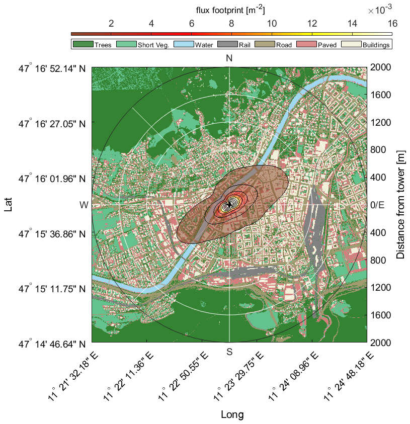
Figure 1 Flux footprint surrounding the IAO tower plotted on top of a gridded land use map derived from OpenStreetMap (© OpenStreetMap contributors 2020. Distributed under a Creative Commons BY-SA License).

NO_x measurements were based on a dual-channel chemiluminescence instrument (CLD 899 Y, ECO PHYSICS). The instrument was operated in flux mode, acquiring data at about 5 Hz. A NO standard was periodically introduced for calibration. Zeroing was performed once a day close to midnight. The chemiluminescent instrument is equipped with a metal oxide (i.e., molybdenum) converter. It has been shown (Steinbacher et al., 2007) that this can result in an overestimation of NO₂ due to decomposition of NO_y species. For Innsbruck we evaluated the accuracy using side-by-side measurements with a cavity ring-down spectrometer in 2015 (Karl et al., 2017). Both independent techniques agreed to within 6 %, confirming that this problem plays a minor role for polluted sites. CO₂ and H₂O were measured with a closed-path eddy covariance system (CPEC200, short inlet, enclosed IRGA – infrared gas analyzer – design, Campbell Scientific) along with three-dimensional winds. Calibration for CO₂ was performed once a day. Aromatic NMVOCs (i.e., benzene, toluene, xylenes and ethylbenzene, and C₉ benzenes) were measured with a PTR-TOF 6000 X2 mass spectrometer (IONICON, Austria), operated in hydronium mode at standard conditions in the drift tube of about 110 Td (Townsend). The instrument was set up to sample ambient air from a turbulently purged $\mathrm{3}/\mathrm{8}$ in. Teflon line. Zero calibrations were performed by providing NMVOC-free air from a continuously purged catalytical converter though a setup of software-controlled solenoid valves. In addition, daily calibrations were performed using known quantities of a suite of NMVOCs from a 1 ppm calibration gas standard (Apel Riemer, USA) that were added to the NMVOC-free air and dynamically diluted into low-ppbv mixing ratios. Errors arising from analytical uncertainty mainly stem from calibration procedures. For NMVOCs these are estimated as 10 % for aromatic-NMVOC compounds based on a calibration standard; similarly the uncertainty of NO_x is 2 %, and that of CO₂ is 5 %, respectively.

This study builds on long-term NO_x and CO₂ flux measurements that have run operationally since 1 June 2018. NMVOC fluxes were measured during a field campaign from 11 March to 9 April 2019 and during the SARS-CoV-2 lockdown, when measurements started on 16 March 2020. The NMVOC analysis presented in this paper spans from 16 March to 1 May 2020.

2.3 Boosted regression tree model

Statistical persistence and regression models have a long history in atmospheric chemistry (Robeson and Steyn, 1990) for predicting empirical trends of pollutants (e.g., ozone) that factor in meteorological and chemical processes. These approaches have been used to forecast local surface ozone (Cobourn, 2007; Prybutok et al., 2000) and more recently trends of other atmospheric pollutants (Grange and Carslaw, 2019). Here we developed a boosted regression tree model using machine learning that is widely used in ecological modeling (Elith et al., 2008): for each variable we based the model on the following key astronomical and environmental driving variables: day of year (DOY), time of day (TOD), weekday or holiday (WDY), cartesian wind vectors (north–south and west–east directions), temperature (T), relative humidity (RH), global radiation (GR), and pressure (P). The model is set up using the machine learning toolbox in MATLAB (MathWorks Inc, USA) and trained for individual datasets until 29 February 2020 or during key reference periods (Table S1 in the Supplement). The model performance was assessed by comparing predicted and observed quantities using reference datasets (Table S2). To obtain a quantitative measure of emission changes, the differences between observed and predicted fluxes are integrated from the beginning of the lockdown period. As the predicted and observed quantities diverge, the integrated relative difference serves as a quantitative measure of emission (or activity) alteration (e.g., reduction).

2.4 Multispecies pollutant model

Based on two major and distinct urban pollution sources (i.e., road traffic and energy production in the residential, public, and commercial sectors) proportional contributions to the observed flux changes can be attributed based on a two-end-member mixing model: traffic emissions are primarily related to exhaust from internal combustion engines. The Austrian passenger car fleet is comprised of 43 % gasoline- and 55 % diesel-driven cars (Statistik Austria, 2019, http://www.statistik.at, last access: 30 January 2021), with the latter being a key player for urban NO_x emissions. The second significant emission source stems from fossil energy production in the residential, public, and commercial sectors with a significant contribution of natural gas combustion. In its simplest form we can therefore aggregate the observed flux changes into two main emission source categories using a two-end-member mixing model:

$$\begin{array}{}\text{(4)}& {\displaystyle \frac{\mathit{\delta }F\left(s\right)}{F\left(s\right)}}=a_{\mathrm{s}}\cdot {\displaystyle \frac{\mathit{\delta }T}{T}}+b_{\mathrm{s}}\cdot {\displaystyle \frac{\mathit{\delta }R}{R}}+\mathit{\epsilon },\end{array}$$

where $\frac{\mathit{\delta }F\left(s\right)}{F\left(s\right)}$ is the measured relative flux difference between the output of the boosted regression tree model and the actual flux observations of species s (e.g., NO_x, CO₂, and aromatic NMVOCs), $\frac{\mathit{\delta }T}{T}$ is the traffic load difference determined from traffic count data, $\frac{\mathit{\delta }R}{R}$ is the residential energy consumption change, a_s and b_s are proportionality terms, and ε is an error term. The proportionality terms (a_s and b_s) represent the area weighted emission factors of the fleet average traffic (a_s) and RCP sector (b_s). By definition $a_{\mathrm{s}}+b_{\mathrm{s}}:=\mathrm{1}$, if only two sources are considered.

3 Results

The urban NO–NO₂–O₃ triad. Due to the short atmospheric lifetime (e.g., up to 7 h, Laughner and Cohen, 2019) nitrogen oxides can serve as a gauge to assess air pollution changes as their atmospheric concentrations rapidly respond to shifting surface fluxes. The quantitative assessment of NO_x emissions based on ambient-air concentrations however remains challenging due to non-linearities within the NO–NO₂–O₃ triad in polluted regions (Lenschow et al., 2016). Under sunlight conditions and high NO_x pollution the cycling between the NO–NO₂–O₃ triad is described by the following reaction sequence:

$$\begin{array}{}\text{(5)}& {\displaystyle }& {\displaystyle }{\mathrm{NO}}_{\mathrm{2}}+h\mathit{\nu }\to \mathrm{NO}+\mathrm{O},\text{(6)}& {\displaystyle }& {\displaystyle }\mathrm{O}+{\mathrm{O}}_{\mathrm{2}}\to {\mathrm{O}}_{\mathrm{3}},\text{(7)}& {\displaystyle }& {\displaystyle }\mathrm{NO}+{\mathrm{O}}_{\mathrm{3}}\to {\mathrm{NO}}_{\mathrm{2}}+{\mathrm{O}}_{\mathrm{2}}.\end{array}$$

The chemical timescale of the NO_x triad (Eqs. 5 to 7) can be derived (Lenschow and Delany, 1987) as

$$\begin{array}{}\text{(8)}& {\displaystyle }\mathit{\tau }={\displaystyle \frac{\mathrm{2}}{\sqrt{\left[\begin{array}{c}{j}^{\mathrm{2}}+k_{\mathrm{3}}^{\mathrm{2}}{\left(\left[{\mathrm{O}}_{\mathrm{3}}\right]-\left[\mathrm{NO}\right]\right)}^{\mathrm{2}}\\ +\mathrm{2}j\cdot k_{\mathrm{3}}\left(\left[{\mathrm{O}}_{\mathrm{3}}\right]+\left[\mathrm{NO}\right]+\mathrm{2}\cdot \left[{\mathrm{NO}}_{\mathrm{2}}\right]\right)\end{array}\right]}}}.\end{array}$$

For typical conditions encountered during this study, this equates to timescales of about 100 s, comparable to the vertical turbulent exchange time in cities. Due to the rapid interconversion, the partitioning between NO and NO₂ is typically dominated by fast chemistry, and the bulk of NO₂ in the urban atmosphere is produced secondarily via the reaction of NO and O₃. In the urban atmosphere this leads to a non-linear relationship between NO₂ and NO_x concentrations as depicted in Fig. 2. A repartitioning can be observed during the suppression phase for example, when the NO₂-to-NO_x trajectory moves from an urban NO_x-saturated regime to a more NO_x-limited regime. During the SARS-CoV-2 lockdown this shift was more pronounced than for typical weekend–weekday variations (Fig. 2b and c). As a consequence the relationship between changes of NO_x fluxes and NO₂ concentrations becomes a non-linear function of NO_x concentrations when moving from NO_x-saturated to NO_x-limited conditions. Data from a nearby air quality station support these conclusions, showing significantly different NO_x concentrations during the 2020 lockdown compared to the previous 5 years (i.e., a 50 % reduction of NO_x) but no significant change for O_x ($:={\mathrm{NO}}_{\mathrm{2}}+{\mathrm{O}}_{\mathrm{3}}$) based on the z hypothesis test. This chemical repartitioning and vertical redistribution in the surface layer needs to be accounted for when quantifying changing NO_x emissions from concentrations. A more quantitative picture of changing NO_x emissions can be obtained from direct flux measurements that are intrinsically linked to surface emissions (Vaughan et al., 2016).

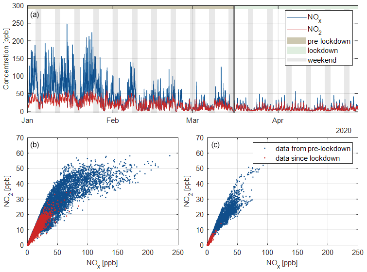
Figure 2 (a) Time series of mixing ratios of ambient NO₂ and NO_x before and during the lockdown. Gray-shaded vertical bars indicate weekends. The gray vertical solid line depicts the start of lockdown measures on 16 March 2020. (b) NO₂ vs. NO_x during weekdays (Tuesday to Thursday). (c) NO₂ vs. NO_x on Sundays.

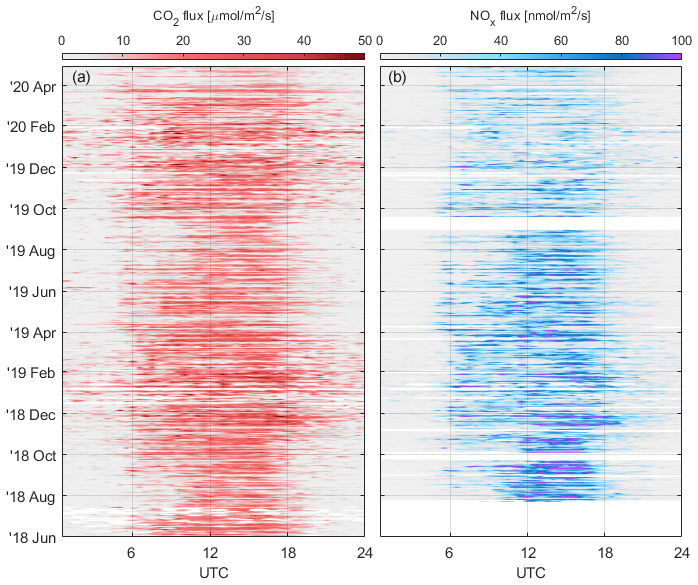
Figure 3 Diurnal variations of CO₂ (a) and NO_x (b) fluxes since 2018. Please note that the date format in this figure is the two-digit year followed by the month.

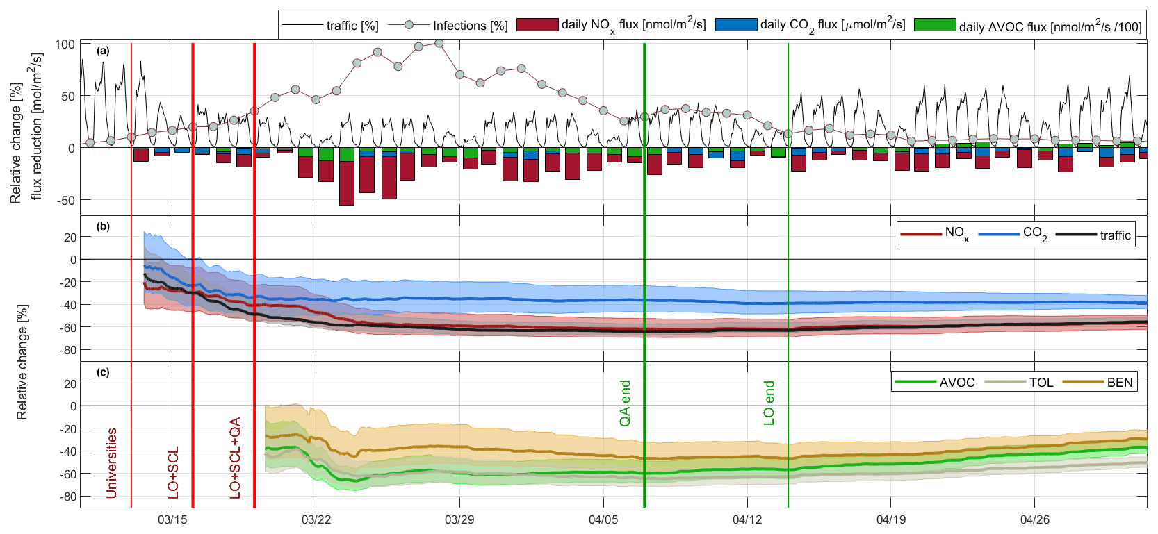
Figure 4 Observed changes of air pollutant fluxes, CO₂ flux, and traffic during the course of the first SARS-CoV-2 wave. (a) Normalized traffic counts, daily infection rate, and daily average flux reduction. (b) Cumulative reduction of NO_x and CO₂ fluxes and traffic activity. (c) Cumulative reduction of aromatic VOCs (AVOCs; volatile organic compounds), toluene (TOL), and benzene (BEN) fluxes. Red vertical lines indicate the start of university closure, Austrian lockdown (LO), school closure (SCL), and quarantine (QA) in the state of Tyrol. Green vertical lines show the lifting of mobility restrictions. Light-shaded areas represent the uncertainty of the boosted regression tree model analysis (Supplement). Please note that the date format in this figure is month day (mm/dd).

Figure 3 gives an overview of NO_x and CO₂ fluxes which have been continuously measured at the study site in central Europe since 2018. In addition, we have performed regular field campaigns augmenting these long-term datasets with NMVOC flux measurements (Karl et al., 2020). While atmospheric concentrations of primary air pollutants often exhibit strong surface maxima due to inversion layers during winter and spring, the corresponding emission fluxes typically track urban emission source activity and reflect changes in emission strengths and flux footprint. Turbulent fluxes typically exhibit midday maxima, reflecting increases in urban emission sources, which in the case of nitrogen oxides closely follow traffic load patterns (Karl et al., 2017). Urban CO₂ fluxes follow these general trends but are to some extent less pronounced (e.g., weekend–weekday effect). During the vegetation period, CO₂ emission fluxes can be suppressed (Ward et al., 2015) due to photosynthetic uptake by urban plants. For Innsbruck, we have assessed this effect previously and find that within the flux footprint the contribution of vegetation is relatively small (i.e., only about 10 % of the urban surface within the flux footprint is covered by plants). Urban CO₂ fluxes are therefore primarily controlled by combustion processes. The flux site is situated in a valley with two dominant wind sectors, which cover a typical inner-city residential and business district (Fig. 1) with no significant industrial activities. In order to quantitatively investigate emission flux changes in response to SARS-CoV-2 intervention measures, we implemented a boosted regression tree model to define a business-as-usual scenario of the observed fluxes (Duffy and Helmbold, 2002). The model allows for factoring in differences in weather patterns (e.g., meteorological variations such as temperature, wind direction, and flux footprint) and describes changes that can be primarily attributed to the intervention itself. Accounting for seasonal differences is key to an accurate analysis of emission alterations due to lockdown measures. The essential time period of pre- and post-lockdown measures in Europe spans from March to about May 2020. Weather patterns in Europe can be particularly variable during this period, as the continent transitions from winter to summer. The climate of Tyrol is fairly representative of central Europe, where the transitional period between March to May can exhibit significant synoptic variability. For example, average monthly temperatures in March 2020 were about 0.9 K colder than in 2019. April and May 2020 tended to be 1.8 and 3.2 K warmer than 2019. Warmer temperatures in spring 2020 resulted in 24 % fewer heating degree days (HDDs) than in the year 2019 (Supplement). Consistent with these observations, natural gas consumption in Tyrol (Supplement) was reported to be 25 % lower during this period than in 2019. We can quantify changes of the observed fluxes due to the lockdown intervention in spring 2020 by referencing actual flux measurements to results from a trained boosted regression tree model (Fig. 4).

Shortly after the European SARS-CoV-2 outbreak first sparked in Italy, which was among the first European countries, the greater part of the Alps was under lockdown by mid-March to inhibit cross-border transmission. Tyrol implemented extensive measures of shelter in place and a state-wide quarantine (QA) on top of the Austrian lockdown (LO) on 16 March, 1 week after all universities closed. At the same time, Europe-wide measures of border control impacted all major north–south transport corridors to Italy. These measures resulted in massively reduced local mobility in combination with significant disruptions of one of the major transport routes across the Alps. As a consequence, average traffic loads in Innsbruck decreased by ∼64 %. The traffic data allow for partitioning traffic into “all vehicles”, “truck-similar vehicles”, “HDVs” (heavy-duty vehicles), and “semi-trailer trucks”. The reductions were 64 % (all vehicles), 40 % (truck-similar vehicles), 35 % (HDVs), and 21 % (semi-trailer trucks). Since it is an inner-city location, the fraction of passenger cars dominate. In absolute numbers, the distribution is dominated by passenger cars (<3.5 t), amounting to 95 % of all traffic, with the remainder attributed to the truck categories. The Austrian rate of infections reached a peak of 900 newly confirmed cases per day in mid-March and started to decline at the end of March. Along with efforts to reduce SARS-CoV-2 transmission, the shelter-in-place legislation resulted in a rapid decline of NO_x, CO₂, and aromatic NMVOCs (benzene, toluene, xylenes and ethylbenzene, and C₉ benzenes) fluxes (Fig. 4a) reaching significantly lower emission fluxes relative to the business-as-usual scenario. The cumulative reduction of surface emissions of air pollutants (NO_x and aromatic NMVOCs) closely follows traffic (Fig. 4b and c), declining by about 64 % during the lockdown period. At the end of the Austrian lockdown, traffic counts and integrated emissions of NO_x and aromatic NMVOCs were −64 %, −59 %, and −56 % lower compared to the business-as-usual scenario. This reduction is significantly lower than observed for CO₂ fluxes, leveling out at about −38 %. Notably benzene emission declines were also less pronounced than toluene and higher aromatic NMVOCs, which track NO_x and traffic loads more closely. These different sensitivities indicate a non-linear relationship between the reduction of carbon dioxide and air pollution gases due to different urban combustion sources. Particularly reductions of NO_x and CO₂ exhibit quite different emission trajectories during the lockdown phase (Fig. 5). The observed reduction of air pollution gases, such as NO_x, is significantly larger than estimated by early bottom-up model predictions for expected NO_x-to-CO₂ emission changes (Le Quéré et al., 2020). Can these observations be reconciled with bottom-up emission projections?

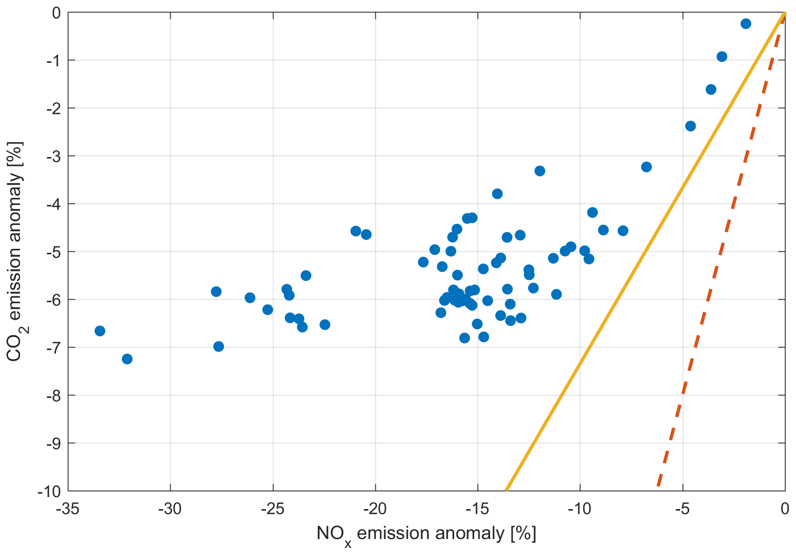
Figure 5 Daily change of CO₂ and NO_x fluxes during the lockdown period. Flux observations are depicted by the blue dots. Emission model projections are represented by the solid orange line (Austrian emission inventory) and the dashed red line (Le Quéré et al., 2020).

4 Discussion

Our analysis indicates that the reduction of classic air pollutant emissions during the SARS-CoV-2 lockdown was more significant than that of CO₂, which comes as a surprise. Comparable to most European countries, Austria-specific bottom-up emission models typically attribute 40 % of CO₂ emissions to traffic and 19 % to the residential, commercial, and public (RCP) sector (UBA, 2019). For NO_x, Austrian and European bottom-up emission projections predict similar contributions (i.e., 58 % from traffic and 12 % from the RCP sector). In its simplest form, by using a two-end-member pollutant model, we can test these assumptions in more detail and compare our observations with an Austrian state-of-the-art emission model (https://www.emikat.at, last access: 30 January 2021) used for national emission reporting. For the analysis we take advantage of the fact that the seasonal influence on pollutant fluxes is factored in by referencing the flux analysis to the trained boosted regression tree model. Further, measured relative reductions of vehicle counts are assumed to represent the decrease of traffic activity reasonably well. We are then left with constraining the intervention-specific changes in the RCP sector. We argue that these must not have changed much because (a) heating appliances are primarily driven by temperature (Z. Liu et al., 2020) (accounted for by our analysis), (b) changes in electricity needs do not enter the local pollutant budget, and (c) less time spent in commercial and public buildings was compensated by more time in residential buildings. Google mobility reports (Alphabet Inc., 2020) based on cell phone tracking suggest a 20 % increase in time spent in the residential sector and a 30 % decrease in the commercial and public sector for Tyrol during the lockdown period. The energy mix in Innsbruck for heating demand is partitioned into residential and “other” (state of Tyrol). The relative contributions to the energy mix for heating in these two broad categories are comparable. In the residential sector it is comprised of 9 % district heating, 34 % oil, 34 % natural gas, 16 % biomass, and 6 % electricity, with the remainder (1 %) being attributed to alternative energy. The category “other” (i.e., everything else) is comprised of 4 % district heating, 37 % oil, 42 % gas, 11 % biomass, and 4 % electricity, with the remainder (2 %) being attributed to alternative energy. Z. Liu et al. (2020) estimated a decline of commercial and residential emissions by 3.6 %; Le Quéré et al. (2020) assumed an increase of residential emissions by 4 % and a decrease in the public sector by 33 % for Europe. As a conservative estimate we bracket changes in the RCP sector activity between 0 % and −20 %, with a best estimate based on the local Google mobility index (−10 %). The observed flux changes can then be partitioned into NO_x emissions from vehicular traffic (${\mathrm{94}}_{-\mathrm{11}}^{+\mathrm{2}}\mathit{\%}$) and the RCP sector (${\mathrm{6}}_{-\mathrm{2}}^{+\mathrm{11}}\mathit{\%}$) accordingly. For CO₂, benzene, toluene, and the sum of aromatic NMVOCs we calculate ${\mathrm{59}}_{-\mathrm{10}}^{+\mathrm{7}}\mathit{\%}$, ${\mathrm{70}}_{-\mathrm{7}}^{+\mathrm{5}}\mathit{\%}$, ${\mathrm{94}}_{-\mathrm{11}}^{+\mathrm{2}}\mathit{\%}$, and ${\mathrm{87}}_{-\mathrm{11}}^{+\mathrm{2}}\mathit{\%}$ arising from vehicular traffic emissions and ${\mathrm{41}}_{-\mathrm{11}}^{+\mathrm{7}}\mathit{\%}$, ${\mathrm{30}}_{-\mathrm{8}}^{+\mathrm{5}}\mathit{\%}$, ${\mathrm{6}}_{-\mathrm{1}}^{+\mathrm{11}}\mathit{\%}$, and ${\mathrm{13}}_{-\mathrm{3}}^{+\mathrm{2}}\mathit{\%}$, respectively, coming from the RCP sector. These results suggest that NO_x is dominated by vehicular traffic emissions and that CO₂ is partitioned more equally between the traffic and RCP sectors. In contrast, urban NMVOC emissions are generally more diverse (Karl et al., 2018). Here we investigate aromatic NMVOCs, which are closely linked to combustion processes and fossil fuel use (EPA, 1998). We observe that toluene and higher aromatic NMVOCs closely track reductions of NO_x emissions and vehicular traffic activity. Benzene declined less readily, suggesting that benzene emissions could be more prevalent from the RCP sector. Speciated NMVOC emission factors from residential gas and oil combustion are still quite uncertain, but recent reports from shale gas operations in the US for example indicate a higher contribution of benzene than toluene emissions from natural gas combustion when compared to traffic sources (Gilman et al., 2013; Halliday et al., 2016; Helmig et al., 2014).

After mapping NO_x and CO₂ emissions from a spatially disaggregated emission model on the seasonal flux footprint (Supplement), the observationally inferred results from above can be compared to the relative attribution of inventory-based emission projections. As for NO_x and CO₂, the official local bottom-up emission inventory apportions 78 % of NO_x fluxes coming from vehicular traffic and 21 % from the RCP sector. For CO₂ these relative contributions are 54 % (traffic sector) and 46 % (RCP sector), respectively. These inventory-based results are roughly in line with a recently published bottom-up assessment for CO₂ emissions (Le Quéré et al., 2020). We also find that CO₂ fluxes are consistent with the relative emission attribution in the inventory but that NO_x emissions are significantly overestimated from the RCP sector (e.g., 21 % vs. 6 %) in favor of traffic (Fig. 4). This suggests cleaner NO_x combustion sources in the RCP sector and higher NO_x emissions from the traffic sector.

The European gas demand has increased significantly over the past decades (European Commission, 2020). As an example, consumption of natural gas increased by about a factor of 4 in Austria (Statistik Austria, 2019) since 1965 and has expanded to 9×10⁹ m³. Across Europe growing demand has increased dependence on gas imports, triggering fierce competition between major gas-producing nations (European Commission, 2020). Apart from the power sector, residential demand has contributed significantly to the overall consumption growth across Europe (European Commission, 2020). While residential gas consumption per inhabitant varies quite drastically across European countries, many countries have invested in developing the residential sector towards a higher fraction of natural gas by fuel subsidy policies. Particularly urban areas, where gas infrastructure is in place, have seen significant growth. As an example, the residential energy sector has seen a doubling of the natural gas share for space-heating appliances in western Austria over the last 9 years (Statistik Austria, 2019). In parallel, oil consumption and solid fuel consumption have decreased by about 40 % in the residential sector over the same period. On average, gas represents about a third of the final energy consumption in the residential sector in Austria and across Europe (European Commission, 2020). One of the reasons for promoting natural gas through subsidies in the past was that gas combustion releases about 25 % less CO₂ than oil and 40 % less than solid fuels (IEA, 2020). In addition to more efficient energy production, natural gas combustion releases fewer air toxins, such as NO_x, CO, NMVOCs, and SO₂, when compared to biomass and other solid fuels (EEA, 2019). However, emissions from the RCP sector are quite uncertain and often rely on Tier 1 upscaling methodology (Blain et al., 2019; EEA, 2019). As the European community is committed to transitioning to a carbon-neutral economy (OECD/IEA/NEA/ITF, 2015), the air quality benefit from natural gas in the residential sector needs to be considered, particularly when introducing renewable alternatives such as wood and pellet combustion on a large scale. Our data suggest that the air quality benefit for the release of reactive nitrogen in the RCP sector might have been underestimated in bottom-up emission inventories used for policy making. Official inventory data show that the increase of natural gas combustion in the RCP sector played a significant role in Europe's energy policy. Wood combustion on the other hand would release significant amounts of reactive nitrogen in the gas and aerosol phase depending on fuel N content (Roberts et al., 2020). While pellet combustion is considered cleaner than wood combustion, Tier 1 emission factors for NO_x are still about twice as high compared to natural gas combustion, and the release of aerosols is of particular concern (EEA, 2019). When transitioning to a climate-neutral economy, the air quality penalty arising from some renewables needs to be sustainable. From the present analysis we find that the biggest gain for the reduction of urban NO_x in Europe remains in the mobility sector and that NO_x emissions from the RCP sector are significantly lower than expected. Europe's push towards a diesel-driven car fleet has helped to curb CO₂ emissions in the mobility sector but created excess emissions of nitrogen oxides. While the extent of cheating devices used in cars to simulate lower than actual NO_x emissions is still unraveling, aggressive reductions of nitrogen oxides are needed to meet Europe's air quality goals (EU-EUR-Lex, 2008). A significant NO_x emission reduction in the mobility sector could help counteract potential increases of air pollutants from promoted renewables such as biomass combustion in the future. Urban eddy flux methods present a top-down methodology allowing for quantifying and testing urban sustainability goals of air pollution and climate gas emissions. In combination with an intervention experiment as shown here they can provide a unique and independent verification method of anticipated air quality and climate policy targets.