Technical note: First comparison of wind observations from ESA's satellite mission Aeolus and ground-based radar wind profiler network of China

Aeolus is the first satellite mission to directly observe wind profile information on a global scale. After implementing a set of bias corrections, the Aeolus data products went public on 12 May 2020. However, Aeolus wind products over China have thus far not been evaluated extensively by ground-based remote sensing measurements. In this study, the Mie-cloudy and Rayleigh-clear wind products from Aeolus measurements are validated against wind observations from the radar wind profiler (RWP) network in China. Based on the position of each RWP site relative to the closest Aeolus ground tracks, three matchup categories are proposed, and comparisons between Aeolus wind products and RWP wind observations are performed for each category separately. The performance of Mie-cloudy wind products does not change much between the three matchup categories. On the other hand, for Rayleigh-clear and RWP wind products, categories 1 and 2 are found to have much smaller differences compared with category 3. This could be due to the RWP site being sufficiently approximate to the Aeolus ground track for categories 1 and 2. In the vertical, the Aeolus wind products are similar to the RWP wind observations, except for the Rayleigh-clear winds in the height range of 0–1 km. The mean absolute normalized differences between the Mie-cloudy (Rayleigh-clear) and the RWP wind components are 3.06 (5.45), 2.79 (4.81), and 3.32 (5.72) m/s at all orbit times and ascending and descending Aeolus orbit times, respectively. This indicates that the wind products for ascending orbits are slightly superior to those for descending orbits, and the observation time has a minor effect on the comparison. From the perspective of spatial differences, the Aeolus Mie-cloudy winds are consistent with RWP winds in most of east China, except in coastal areas where the Aeolus Rayleigh-clear winds are more reliable. Overall, the correlation coefficient R between the Mie-cloudy (Rayleigh-clear) wind and RWP wind component observation is 0.94 (0.81), suggesting that Aeolus wind products are in good agreement with wind observations from the RWP network in China. The findings give us sufficient confidence in assimilating the newly released Aeolus wind products in operational weather forecasting in China.

1 Introduction

Observations of atmospheric wind profiles are essential to the prediction of extreme rainfall events (Nash and Oakley, 2001; Huuskonen et al., 2014; King et al., 2017), the forecasting of tropical cyclones and hurricanes (Pu et al., 2010; Stettner et al., 2019), a better understanding of persistent haze pollution episodes (Liu et al., 2018; Yang et al., 2019; Zhang et al., 2014, 2020; Huang et al., 2020), and complicated aerosol–cloud–precipitation interactions (Li et al., 2011; Lebo and Morrison, 2014; Guo et al., 2018, 2019; Huang et al., 2019; Shi et al., 2020). Moreover, under the influence of large-scale dynamic forcing and land surface processes, wind speed and direction will vary dramatically, both temporally and spatially, which poses a large challenge for models to simulate or forecast the variation in wind very well (Weissmann et al., 2007; Michelson and Bao, 2008; Constantinescu et al., 2009). Particularly, the winds in the atmospheric boundary layer are mostly turbulent and hard to be well reproduced by models without assimilation of wind observations (Belmonte and Stoffelen, 2019; Benjamin et al., 2004; Simonin et al., 2014; Liu et al., 2017; Stoffelen et al., 2019). Therefore, continuous global wind profile observations are of great significance for advancing our knowledge of atmospheric dynamics as well as for improving the accuracy of numerical weather prediction (Stoffelen et al., 2005).

To this end, various instruments have been developed to measure wind speed and direction, including radiosondes, radar wind profilers (RWPs), and geostationary satellites (Stoffelen et al., 2019; Bentamy et al., 1999; Draper and Long, 2002; Guo et al., 2016; Liu et al., 2019). Among others, radiosonde measurements are one of the most widely used observations for atmospheric wind profiles (Houchi et al., 2010). Radiosondes can directly measure vertical profiles of thermodynamic and dynamic parameters, including pressure, temperature, humidity, and horizontal winds. Nevertheless, the launch frequency of operational radiosonde balloons is not high, only once or twice a day (Guo et al., 2016), and spatially sparse. Therefore, the advantage of the use of RWPs for characterizing the temporal variability in the wind is its continuous and unattended operation (Liu et al., 2020a; Zhang et al., 2020). However, the operational and maintenance costs are extremely high, and the spatial coverage (both vertically and horizontally) is still limited, such that operation of most of the nationwide radar wind profiler (RWP) networks has stopped, except in China (Guo et al., 2016; Liu et al., 2020b). In comparison, a spaceborne Doppler wind lidar (DWL) is increasingly considered one of the most promising instruments to meet the need of near-real-time observations, mostly thanks to its global coverage (Stoffelen et al., 2020; Zhai et al., 2020).

Aeolus, launched on 22 August 2018, is the first ever satellite designed to directly observe line-of-sight wind profiles on a global scale (Stoffelen et al., 2005; Witschas et al., 2020; Zhai et al., 2020). The unique payload, the Atmospheric Laser Doppler Instrument (ALADIN), is a direct-detection ultraviolet wind lidar operating at 355 nm (Reitebuch, 2012; ESA, 2016). It uses a dual-channel design, which can simultaneously obtain the particulate and molecular backscatter from Mie and Rayleigh channels, respectively. Aeolus provides one component of the wind vector along the instrument's line of sight (Stoffelen, 2005). The Aeolus dataset has gone through bias correction procedures and has been available publicly to forecasting services and scientific users since 12 May 2020. Currently, the products that are entirely publicly accessible are the Level-1B and Level-2B products. Here, the Level-2B products containing the horizontal line-of-sight (HLOS) wind observations are used. The Level-2B product provides the scientific wind product for users, which is the geo-located and consolidated HLOS wind observation with actual atmospheric correction and bias corrections applied (Tan et al., 2017; Rennie et al., 2018).

To estimate the performance of the Aeolus wind products, the Aeolus team has performed extensive experimental (e.g., Witchas et al., 2010) and simulation (Marseille et al., 2003; Stoffelen et al., 2005) studies, which were complemented by a series of airborne DWL measurements (Lux et al., 2018; Marksteiner et al., 2018; Witschas et al., 2020). The first validation of the Aeolus Level-2B product was performed against the European Centre for Medium-Range Weather Forecasts (ECMWF) numerical weather prediction (NWP) model, which played a crucial role in the Aeolus characterization (Rennie and Isaksen, 2020). Validation against in situ airborne DWL measurements was conducted by Witschas et al. (2020). They analyzed the systematic and random errors in the Aeolus wind products and confirmed the necessity to validate the Aeolus wind product. Lux et al. (2020) compared the wind observations from Aeolus and the ALADIN Airborne Demonstrator (A2D) with the ECMWF NWP winds and found that the biases of the A2D and Aeolus line-of-sight wind speeds were −0.9 and +1.6 m/s, respectively, while the random errors were around 2.5 m/s. In a triple collocation, Albertema (2019) used a spatially dense airplane network for in situ verification of Aeolus wind profiles. The abovementioned verification exercises have deepened our understanding of the global Aeolus wind products, and most of the biases have now been corrected in the newest Level-2B (L2B) Aeolus product release (see next section). It is noted that most in situ verifications were conducted over Europe. Over countries or regions with episodes of extensive heavy air pollution, such as China, the high aerosol concentrations could affect satellite observations, which in turn can potentially affect the accuracy of wind products and their applications in weather forecast and climate prediction. In particular, in an atmosphere fraught with dense smoke, dense fog, and haze, the laser energy would be attenuated, making it likely not to well obtain near-surface observation signals (Winker et al., 2009). Moreover, when the aerosol scattering signal is too strong, the molecular scattering signal will be dramatically attenuated, thereby undermining the inversion of Rayleigh wind (Tan et al., 2008, 2017). For instance, many previous studies have shown that China experienced several episodes of severe haze pollution during the COVID-19 lockdown period, despite the widespread emission reduction (Huang et al., 2020; He et al., 2020; Le et al., 2020; Su et al., 2020). For this reason, among others, it is worthwhile extending the in situ verification of the performance of Aeolus wind products to China.

In this study, the quality of the Aeolus wind products over China is investigated by comparing them with the wind observations from the RWP network in China. For the comparison of the RWP measurements with the Aeolus results, the RWP sites are divided into three categories according to the geographic coordinates of each RWP site relative to the nearest Aeolus ground track categories. The HLOS wind profile differences between Aeolus and RWP winds are analyzed for each site. The paper is organized as follows. First, the Aeolus and RWP data used in this study are briefly described, and the data matching algorithms are addressed in detail in Sect. 2. The subsequent sections present a comprehensive comparison between the Aeolus wind products and the RWP wind observations. In Sect. 4, the main findings are summarized.

2 Data and methods

2.1 Aeolus wind observations

Aeolus is the first mission to acquire atmospheric wind profiles on a global scale, deploying the satellite-borne DWL system ALADIN (Stoffelen et al., 2005; ESA, 2008; Reitebuch, 2012). Aeolus flies in a sun-synchronous orbit at an altitude of about 320 km, with a 7 d repeat cycle. The ground tracks of Aeolus over China are shown in Fig. 1. The red and blue lines represent the ascending and descending ground tracks at 06:00 and 18:00 local solar time (LST), respectively. The Aeolus L2B wind product data are the mission's prime and are increasingly receiving attention. Typically, the Aeolus wind profiles from the ground up to a 30 km altitude refer to the wind vector component along the instrument's line of sight, with a vertical resolution of 0.25 to 2 km and a wind accuracy of 2 to 4 m/s, depending on the altitude (Rennie et al., 2020). In this study, the Aeolus L2B products from 20 April to 20 July 2020 have been collected for comparison with RWP observations. They contain the HLOS winds for the Mie and Rayleigh channels. The auxiliary data, such as validity flag, estimated error, and top and bottom altitudes of the vertical bin, are also given in the Aeolus L2B product. The wind speed is calculated based on the Doppler effect (Tan et al., 2008). Here, we mainly discuss the performance of Rayleigh-clear winds and Mie-cloudy winds. Rayleigh-clear winds refer to the wind observations in aerosol-free atmosphere. Mie-cloudy winds refer to the winds acquired from Mie backscatter signals induced by aerosols and clouds (Witschas et al., 2020). The quality of the Aeolus wind data is indicated by validity flags (0 is invalid, and 1 is valid) and estimated errors (theoretical). The estimated error is a theoretical value, which is estimated based on the measured signal levels as well as on the temperature and pressure sensitivity of the Rayleigh channel response (Dabas et al., 2008). It was provided as an indispensable parameter in the L2B data product. More detailed descriptions have been provided in previous studies (De Kloe et al., 2017; Tan et al., 2017).

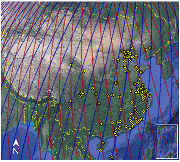
Figure 1 Geographic distribution of RWP sites and Aeolus ground tracks superimposed on a Google Earth map of China (© Google Maps). Red and blue lines represent the Aeolus ground tracks for ascending and descending orbits, respectively. The yellow dots denote the RWP sites.

2.2 RWP wind observations

The RWP network in China is operated and maintained by the China Meteorological Administration. It comprised 134 stations as of April 2020 and is designed primarily for measuring winds at various altitudes (Liu et al., 2020b). The RWP can almost continuously operate (24 h a day, 7 d a week), acquiring vertical profiles of horizontal wind speed, wind direction, and vertical velocity over the station (Zhang et al., 2016; Liu et al., 2019). The temporal and spatial vertical resolutions of RWP data are 6 min and 120 m, respectively. The maximum detection height ranges from 3 to 10 km. The quality flag of the data is based on the confidence level; that is, a 100 % confidence level indicates that the data are valid (Liu et al., 2020b). It should be noted that only about 2 % of RWP measurements were removed for further analysis here, and more detailed information on the RWP network and its data quality can be found in Liu et al. (2020b). Due to the fact that the distance between adjacent tracks of Aeolus is relatively large, subsequent processes are applied to screen the RWP sites. The sites that are more than 1^∘ away from the Aeolus ground track are removed. Following this procedure, 109 stations were selected for comparison with Aeolus data (yellow dots in Fig. 1). For each of these stations, the horizontal wind speed and direction measured during the period from 20 April to 20 July 2020 were obtained to compare them with the results from Aeolus.

2.3 Data matching procedures

Regarding the different spatial–temporal resolutions of RWP and Aeolus, data matching procedures are necessary before comparing. A flowchart of the procedures is shown in Fig. 2. First, the RWP data and Aeolus data need to be matched in both time and space. To achieve a synchronization, the time difference between the RWP and Aeolus wind profiles is required to be less than 10 min. Meanwhile, referring to the well-established geographical matching principle (Zhang et al., 2016), the distance between an Aeolus wind profile and an RWP site should be less than 75 km. After temporal and spatial collocation, the closest Aeolus observation to each RWP measurement is adopted for a comparison.

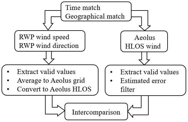
Figure 2 Flowchart of the processing procedures used to compare the RWP observations with Aeolus observations.

In a next step, the valid RWP wind speed and direction are extracted from the wind profile when the data have a 100 % confidence level (Liu et al., 2020b). Moreover, by matching the lowest and highest extracted RWP data with Aeolus, the overlapping wind profiles are selected. In addition, when the altitude coverage of RWP cannot completely match the detection range of the Aeolus, which is typically from 0 to 30 km, a threshold for the number of available RWP observations within an Aeolus bin has to be set. For each Aeolus vertical bin, all of the heights should be covered by RWP measurements. The RWP wind vector in each bin is then projected onto the Aeolus HLOS using the following equation (Witschas et al., 2020):

$$\begin{array}{}\text{(1)}& v_{{\mathrm{RWP}}_{\mathrm{HLOS}}}=\cos \left({\mathit{\psi }}_{\mathrm{Aeolus}}-{\mathrm{wd}}_{\mathrm{RWP}}\right)\cdot {\mathrm{ws}}_{\mathrm{RWP}},\end{array}$$

where ψ_Aeolus represents the Aeolus azimuth angle which is given by the Aeolus L2B data product and ws_RWP and wd_RWP are the RWP wind speed and direction, respectively. For further comparison, the $v_{{\mathrm{RWP}}_{\mathrm{HLOS}}}$ values in each bin are averaged to compare with Aeolus HLOS winds.

In addition, the Aeolus winds are acceptable only when the validity flag equals 1 and the estimated errors for wind are less than 7 and 5 m/s for Rayleigh and Mie channels, respectively. The flag and error information are provided as parameters in the L2B data product, and the error is estimated based on the measured signal levels as well as on the temperature and pressure sensitivities of the Rayleigh channel response (Dabas et al., 2008). Figure S1 shows the scatterplots of Aeolus wind speed against RWP wind speed for all data without controlling the quality using estimated errors. It can be found that the correlation is very poor. Therefore, the official documentation and references pointed out that the estimated errors need to be considered when performing data quality control. The selection of the thresholds is described in detail in the next section.

A case study of comparison between the Aeolus wind measurements and RWP wind observations on 28 April 2020 is presented in Fig. 3, which is superimposed on a Google Earth map of east China where the Aeolus ground track is marked as white circles and the track passes through nine RWP sites. The top and middle panels show the Aeolus Mie-cloudy and Rayleigh-clear winds that pass the valid flag and estimated error selection procedures. The bottom panel displays the corresponding RWP winds matched to the Aeolus Rayleigh-clear measurement grid. It is noted that the horizontal resolution (available observations) of the Mie-cloudy wind products is finer (higher) than that of the Rayleigh wind products. Most of the RWP wind observations are consistent with the Rayleigh wind measurements.

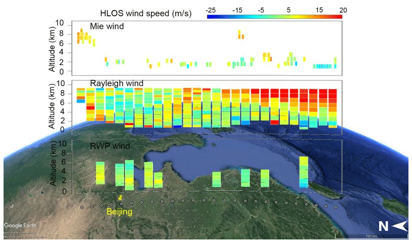
Figure 3 Case study of HLOS wind component profiles on 28 April 2020 between 21.5 and 43.5^∘ N superimposed on the Google Earth map of east China (© Google Maps). The top, middle, and bottom panels show Mie-cloudy, Rayleigh-clear, and RWP wind profiles, respectively. The color bar represents the HLOS wind vector component in meters per second.

2.4 Statistical method

The HLOS difference between Aeolus HLOS winds ($v_{{\mathrm{Aeolus}}_{\mathrm{HLOS}}}$) and the corresponding $v_{{\mathrm{RWP}}_{\mathrm{HLOS}}}$is given by

$$\begin{array}{}\text{(2)}& v_{\mathrm{diff}}=v_{{\mathrm{Aeolus}}_{\mathrm{HLOS}}}-v_{{\mathrm{RWP}}_{\mathrm{HOLS}}}.\end{array}$$

Following Witschas et al. (2020), Aeolus winds with a large estimated error should be removed prior to their use in our analysis. A sensitivity analysis is conducted to choose a suitable threshold for the estimated value of error (Fig. 4). For both Mie-cloudy and Rayleigh-clear winds (Fig. 4a, b), the v_diff between RWP and Mie-cloudy winds is within a rather small margin for estimated errors smaller than 7 m/s and increases with increasing error for higher values. In particular, the v_diff between RWP and Rayleigh-clear winds is rather constant when the error is less than 10 m/s and increases remarkably for the error exceeding 10 m/s. Therefore, referring to the previous threshold standard (Witschas et al., 2020), the selected threshold value for the error is 5 m/s for Mie-cloudy wind and 7 m/s for Rayleigh-clear wind.

Figure 4 Difference between the Aeolus HLOS and RWP HLOS wind components as a function of estimated errors for (a) Mie-cloudy winds and (b) Rayleigh-clear winds. Gray areas indicate the data with errors larger than 7 m/s (Rayleigh) or 5 m/s (Mie), which in the present analysis are considered invalid observations.

The number of samples is limited, which may affect the statistical significance of the comparative results. Therefore, to better evaluate the performance of $v_{{\mathrm{Aeolus}}_{\mathrm{HLOS}}}$, the Aeolus–RWP HLOS differences are normalized by dividing by the theoretical standard deviation (SD) of Aeolus estimated error. It can be expressed by

$$\begin{array}{}\text{(3)}& v_{\mathrm{N}\mathrm{\_}\mathrm{diff}}=v_{\mathrm{diff}}/{\mathrm{SD}}_{\text{estimated error}}.\end{array}$$

Moreover, to evaluate the comparative results, the mean difference (MD) and SD of v_{N_diff} are estimated according to

$$\begin{array}{}\text{(4)}& \mathrm{MD}={\displaystyle \frac{\mathrm{1}}{n}}{\sum }_{i=\mathrm{1}}^n{v}_{\mathrm{N}\mathrm{\_}\mathrm{diff}}\end{array}$$

and

$$\begin{array}{}\text{(5)}& \mathrm{SD}=\sqrt{{\displaystyle \frac{\mathrm{1}}{n-\mathrm{1}}}{\sum }_{i=\mathrm{1}}^n(v_{\mathrm{N}\mathrm{\_}\mathrm{diff}}-\mathrm{MD}{)}^{\mathrm{2}}},\end{array}$$

where v_{N_diff} is the normalized difference between Aeolus and RWP HLOS wind speed. The correlation coefficient (R) between RWP and Aeolus winds is calculated by

$$\begin{array}{}\text{(6)}& R={\displaystyle \frac{{\sum }_{i=\mathrm{1}}^n\left(x_i-\stackrel{\mathrm{‾}}{x}\right)\left(y_i-\stackrel{\mathrm{‾}}{y}\right)}{\sqrt{{\sum }_{i=\mathrm{1}}^n{\left(x_i-\stackrel{\mathrm{‾}}{x}\right)}^{\mathrm{2}}}\sqrt{{\sum }_{i=\mathrm{1}}^n{\left(y_i-\stackrel{\mathrm{‾}}{y}\right)}^{\mathrm{2}}}}},\end{array}$$

where x_i and y_i represent the ith sample point of Aeolus and the RWP wind speed dataset, respectively. The terms $\stackrel{\mathrm{‾}}{x}$ and $\stackrel{\mathrm{‾}}{y}$ represent the mean wind speed of Aeolus and the RWP wind speed dataset, respectively.

3 Results and discussion

3.1 Comparison of Aeolus and RWP wind observations

Scatterplots of Aeolus wind speed against RWP wind speed for Mie-cloudy winds and Rayleigh-clear winds at different times are presented in Fig. 5. The blue and red dots represent the Mie-cloudy and Rayleigh-clear winds, respectively. The Aeolus data were recorded from April to July 2020 and provide 817 (2430) samples for comparison of Mie-cloudy (Rayleigh-clear) and RWP winds with RWP observations. Figure 5a–c show that the slopes of linear fits of Mie-cloudy vs. RWP winds are 1.01, 0.9, and 1.04 for all data, ascending orbits, and descending orbits, respectively. R values between Mie-cloudy and RWP winds are 0.94, 0.9, and 0.9 for all data, ascending orbits, and descending orbits, respectively. These results indicate that the Aeolus Mie-cloudy wind products are broadly consistent with RWP wind observations over China. Figure 5d–f illustrate that for Rayleigh-clear winds, the slopes of linear fit (values of R) are 0.91 (0.74) and 0.96 (0.72) for ascending and descending orbits, respectively. Overall, for all data, the slopes of the linear fits and the R values for the Rayleigh-clear winds are 0.99 and 0.81, respectively. These results indicate that the performance of the Aeolus Rayleigh-clear wind products is reliable over China. It also finds that the performance of Mie-cloudy wind products is superior to that of Rayleigh-clear wind products. In addition, it is interesting to note that most of the wind speeds are positive during the ascending orbit and negative during the descending orbit, due to the predominant westerly wind component.

Figure 5 Aeolus against RWP HLOS winds for (a, b, c) Mie-cloudy winds and (d, e, f) Rayleigh-clear winds for (a, d) all data and (b, e) ascending and (c, f) descending orbits. Corresponding least-square line fits are indicated by the solid lines. The fit results are shown in the insets. The 1:1 line is represented by the gray dashed line.

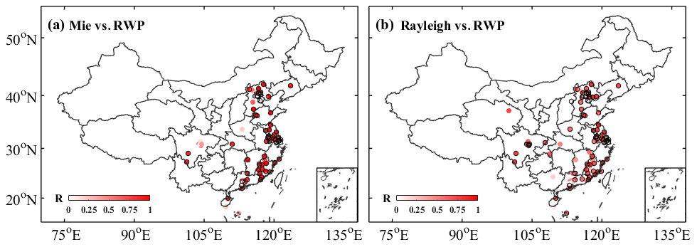
Figure 6 Correlation coefficients between Aeolus HLOS and RWP HLOS wind speeds. The wind measurements are separated in (a) Mie-cloudy winds and (b) Rayleigh-clear winds. The black circles indicate that the site passed the significance test (P<0.05).

The correlation coefficients between the Aeolus and RWP winds for each site are shown in Fig. 6, in which black-outlined circles denote the sites that pass the significance test (P<0.05). It is noted that for some sites the number of valid samples is smaller than five which is too small for a statistically valid comparison. Ultimately, we obtain the spatial distribution of the number of paired data samples, which is shown in Fig. S2. For Mie-cloudy wind products, a total of 72 sites can provide the comparison result, and 53 of them have a correlation coefficient (R) exceeding 0.8, thus indicating that the Aeolus Mie-cloudy wind products are consistent with RWP wind observations in most regions of east China. For the Rayleigh-clear wind products, 89 sites provide comparison results, but for only 27 % of them is R larger than 0.8, and for 70 % R is larger than 0.6. This indicates that the performance of the Aeolus Rayleigh-clear wind products is lower than that of Mie HLOS winds, as found elsewhere too (Rennie and Isaksen, 2020). The geographical distribution in Fig. 6b shows that the sites with high R values are mainly located in coastal areas where economic development is much faster. These results indicate that the HLOS distributions may be wider in the coastal regions, leading to higher correlations. Therefore, the reason for the high R values observed here could be the sufficient maintenance of the RWP instrument along the coastal region, resulting in more matched data points therein (Fig. S2).

3.2 RWP station type

According to the geographic location of each RWP site relative to its nearest Aeolus ground tracks, all the RWP sites are divided into three categories, as shown in Fig. 7, in which the red triangle represents the RWP site and the black circle shows an area with a radius of 75 km centered on the RWP site. Category 1 demonstrates the RWP sites matched two Aeolus ground tracks, with the nearest distance between the RWP site and the Aeolus ground track less than 37.5 km. In addition, category 2 denotes the RWP sites matched by one Aeolus ground track, with the nearest distance less than 37.5 km. Category 3 is the same as category 2 except that the nearest distance is larger than 37.5 km. From all 109 RWP sites, 39 can be attributed to category 2, indicating that 36 % of the RWP sites closely match up with the Aeolus profiles based on their shortest distance of less than 37.5 km. In contrast, categories 1 and 3 have fewer matchups, i.e., 32 sites (29 %) for category 1 and 38 sites (35 %) for category 3. The details of the classification criteria are tabulated in Table 1, in which the number of Aeolus ground tracks, RWP sites, and the shortest distance between them are summarized.

Figure 7 Schematic diagrams of three categories showing the location of Aeolus ground tracks relative to the RWP sites which are based on a circle with a radius of 75 km centered at the RWP sites (red triangle) to match the Aeolus and RWP wind observations: (a) category 1, (b) category 2, and (c) category 3, in which the shortest distance from the ascending (red line) or descending (blue line) Aeolus ground track to its nearest RWP site is less or greater than 37.5 km.

Table 1 Summary of the collocation categories used in this study: position of RWP sites relative to the nearest Aeolus ground tracks, calculated based on a 75 km radius circle centered at each RWP site.

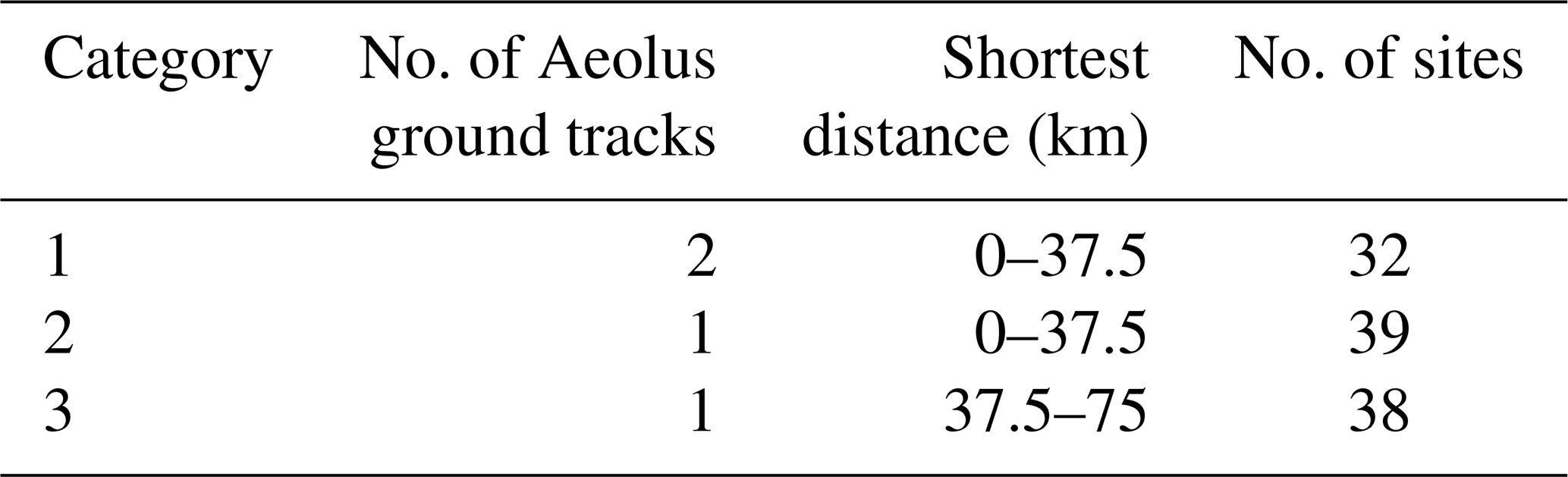
Figure 8 shows the geographic locations of the RWP sites for categories 1, 2, and 3 (magenta, green, and blue solid circles are for 1, 2, and 3, respectively). It is notable that the geographical distributions of categories 1 and 3 are broadly scattered across central and eastern China but category 2 is more predominant over the coastal areas. In addition, we note that the shortest distances in categories 1 and 2 are both less than 37.5 km, and therefore, in total 71 sites with a sufficient approximation to the Aeolus ground tracks are available weekly. This condition indicates that the RWP network in China is well suited for comparison with Aeolus observations.

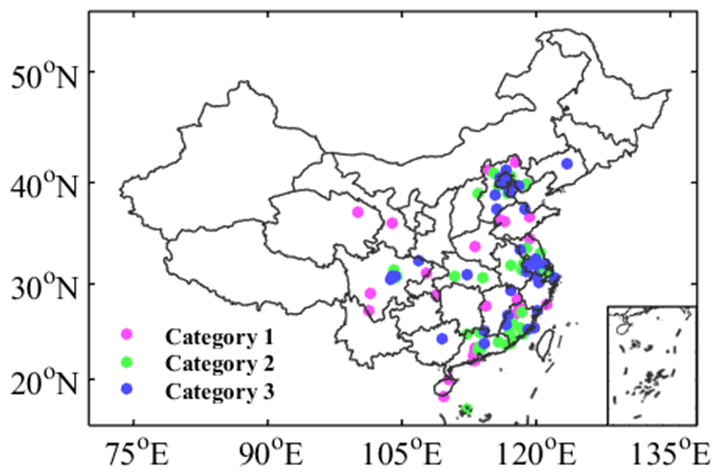
Figure 8 Geographical distribution of RWP sites relative to Aeolus ground tracks over China. The magenta, green, and blue solid circles correspond to categories 1, 2, and 3 as displayed in Fig. 7.

3.3 Differences between Aeolus and RWP winds

The wind speed normalized differences between Mie-cloudy winds and RWP winds are shown in Fig. 9. It is noted that some sites cannot provide comparison results due to empty sample points. The text labels represent the mean difference and standard deviation of the normalized differences in each category. For more than half of the sites (52 out of 90, i.e., 58 %), the mean normalized difference is negative, and the mean normalized difference for all sites is $-\mathrm{0.38}\pm \mathrm{4.19}$ m/s, indicating a small underestimation by Aeolus. More specifically, the mean normalized differences for categories 1, 2, and 3 are $-\mathrm{0.33}\pm \mathrm{4.13}$, $-\mathrm{0.26}\pm \mathrm{3.83}$, and $-\mathrm{0.55}\pm \mathrm{4.66}$ m/s, respectively, implying that the maximum normalized difference among the categories could be as large as 9 m/s. The ascending/descending HLOS wind normalized differences are presented in Fig. 9e–f. We note that the Aeolus LOS points to the right of the spacecraft into the dark side of the earth, implying a westward viewing direction in the morning (descending) and an eastward viewing direction in the evening (ascending). In addition, note that the climatological weather conditions are different in the morning and the evening. More than half of the RWP sites (28 out of 50, i.e., 56 %) have positive differences in mean HLOS during ascending, and for most of the sites (37 out of 53, i.e., 70 %) they are negative during the descending orbits. The mean normalized differences are 0.1±3.84 and $-\mathrm{0.83}\pm \mathrm{4.5}$ m/s for ascending and descending observations, respectively, which suggest that the observation time has a minor effect on the performance of Mie-cloudy winds.

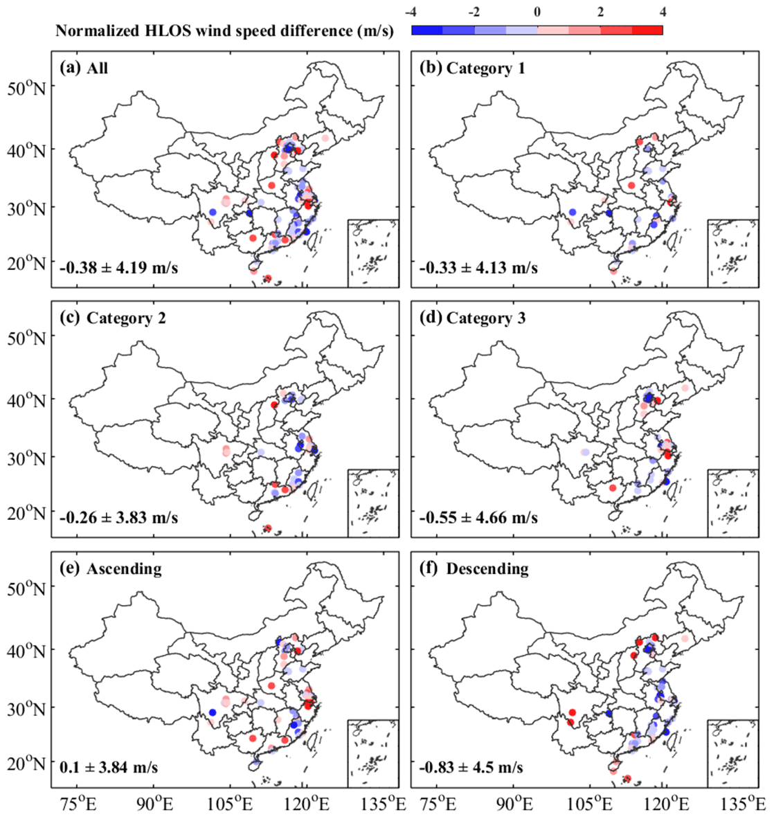
Figure 9 The geographic distribution of the normalized differences between the Aeolus HLOS and the RWP HLOS wind speeds for Mie-cloudy winds. The normalized differences are shown for all RWP sites in China (a) and for the RWP sites belonging to (b) category 1, (c) category 2, (d) category 3, (e) ascending orbits, and (f) descending orbits. The text labels represent the mean difference and standard deviation. The black circles indicate that the site passed the statistical significance difference test (P<0.05).

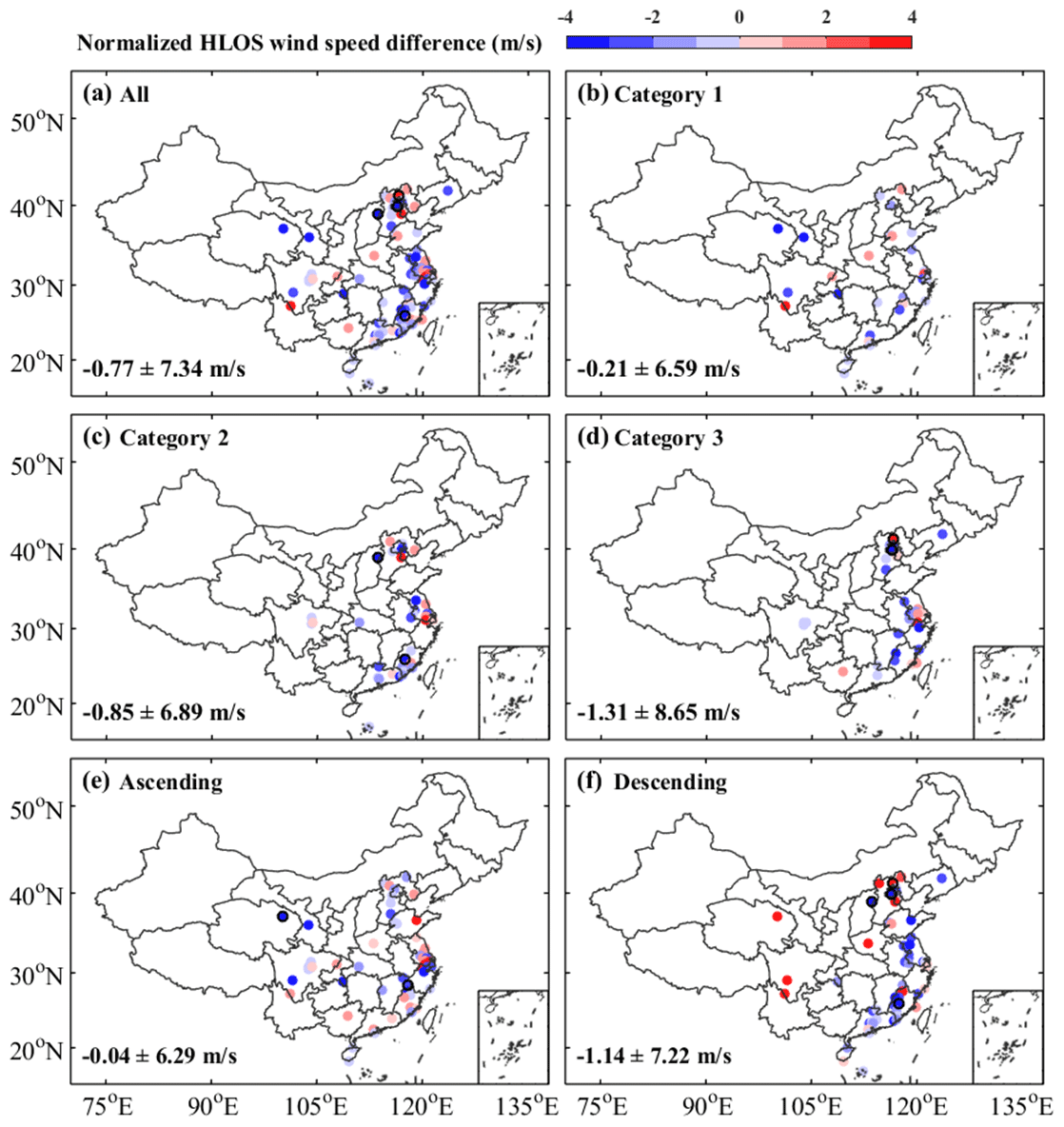
Figure 10 Same as Fig. 9 but for Rayleigh-clear winds.

For Rayleigh-clear winds, the normalized HLOS differences between Aeolus and RWP are presented in Fig. 10. Overall, the Rayleigh-clear winds are a bit underestimated as evidenced by the negative differences for most of RWP sites (66 of out 94, i.e., 70 %) and their mean value over all sites is $-\mathrm{0.77}\pm \mathrm{7.34}$ m/s (statistically insignificant differences). Moreover, the mean normalized difference for Category 3, has a larger magnitude (1.31 m/s), as compared with categories 1 (0.21 m/s) and 2 (0.85 m/s). These differences indicate that the sample size might have some effect on the HLOS differences for the Rayleigh-clear winds. For the ascending orbit, differences at over half of the RWP sites (34 out of 57, i.e., 59 %) have negative values, with a mean of $-\mathrm{0.04}\pm \mathrm{6.29}$ m/s. Similarly, for descending orbits, 71 % of the RWP sites (42 out of 59 sites) have negative values, with a mean of $-\mathrm{1.14}\pm \mathrm{7.22}$ m/s, i.e., statistically insignificant biases. This result moreover indicates that the performance of Rayleigh-clear winds is slightly affected by the observation time.

Figure 11 shows the vertical distribution of the normalized differences between the Aeolus HLOS wind speed and the RWP HLOS wind speed for different categories and times, in which the shaded area represents the standard deviation at different altitudes and the blue and red lines represent Mie-cloudy and Rayleigh-clear winds, respectively. For all observation times, the maximum mean normalized difference between the Mie-cloudy (Rayleigh-clear) winds and the RWP winds is 1.78 (3.23) m/s in the height range of 7–8 (0.3–1) km. Overall, the mean normalized difference between the Mie-cloudy (Rayleigh-clear) winds and the RWP winds is less than 2 m/s in the height range of 1–9 km. These results show that the biases of the Mie-cloudy and Rayleigh-clear wind products are acceptable in the height range of 1–9 km. Note that the Rayleigh-clear wind products have a large difference (3.23±17 m/s) in the height range of 0–1 km. This is due to the Rayleigh performance being limited by received power. Combined with Fig. 11b and c, the vertical distributions of the wind speed normalized differences during ascending and descending orbits are opposite to each other, indicating that the changes in observation time could exert influences on the vertical distribution of the wind speed difference. This may be caused by the diurnal variation in aerosols in the atmospheric boundary layer. At ascending time (06:00 LST), the boundary layer height is generally less than 0.5 km (Guo et al., 2016), and the atmosphere in the range of 0.5–2 km is dominated by molecule scattering. By comparison, at descending time (18:00 LST), the boundary layer height tends to be elevated to approximately 1–2 km, in which aerosol scattering dominates. It is noteworthy that the Rayleigh performance is largely limited by received power. Nevertheless, the strong aerosol scattering in the boundary layer would inevitably undermine the molecular scattering signal, thereby reducing the inversion accuracy of Rayleigh wind from Aeolus (Tan et al., 2017). These conclusions can also apply to the vertical distribution of the differences in all categories. For Mie-cloudy wind products, the normalized differences are underestimated in the region of 7–9 km for categories 1 and 3, while for category 2, they are overestimated in the height range of 7–9 km. Rayleigh-clear wind products are overestimated in the altitude interval of 4–6 km for categories 1 and 2 and underestimated over the full vertical range for category 3. Again, the statistical significance is low.

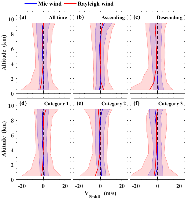
Figure 11 Vertical distributions of the normalized differences between the Aeolus HLOS and RWP HLOS wind speeds for (a) all time, (b) ascending orbits, (c) descending orbits, (d) category 1, (e) category 2, and (f) category 3. Blue and red lines represent Mie-cloudy and Rayleigh-clear wind, respectively. Corresponding color-shaded areas represent 1 standard deviation to each side of the mean normalized difference.

More statistics with regard to the mean absolute normalized difference between Aeolus and RWP winds are presented in Fig. 12. From the perspective of observation time, the mean absolute normalized difference between the Mie-cloudy (Rayleigh-clear) and RWP wind speeds are 3.06±2.89 (5.45±4.97), 2.79±2.64 (4.81±4.06), and 3.32±3.15 (5.72±4.55) m/s for all data, ascending orbits, and descending orbits, respectively. These results suggest that the observation time has a minor effect on the HLOS comparison, and the wind products for ascending orbits is slightly superior to those for descending orbits. As for another relevant variable, i.e., geographic location, the mean absolute normalized differences between the Mie-cloudy and RWP wind speeds are 3.07±2.77, 2.88±2.52, and 3.23±3.39 m/s for categories 1, 2, and 3, respectively. This indicates that the difference in site types has a minor effect on the performance of Mie-cloudy wind products. For Rayleigh-clear wind products, category 3 has the largest difference of 6.2±6.18 m/s between the Rayleigh-clear and RWP wind speed in contrast to small differences of 5.11±4.17 and 5.17±4.62 m/s for categories 1 and 2, respectively, probably indicating that categories 1 and 2 are more suitable to comparing with Rayleigh-clear winds than category 3. The statistical significance difference is also low. Overall, the mean absolute normalized difference (3.06±2.89 m/s) between the Mie-cloudy and RWP wind speeds is smaller than that (5.45±4.97 m/s) between the Rayleigh-clear and RWP wind speeds, indicating that the performance of Mie-cloudy wind products is better than that of Rayleigh-clear wind products. This may be expected from the lower-than-anticipated atmospheric Aeolus return (Kanitz et al., 2020).

Figure 12 Absolute normalized differences between Aeolus HLOS and RWP HLOS wind speeds for Mie-cloudy winds (blue bar) and Rayleigh-clear winds (red bar). The thin black range indicates a spread of absolute normalized difference standard deviations.

4 Conclusions

An initial comparison between the latest version of Aeolus wind products and wind observations from the radar wind profiler network in China during the period 20 April to 20 July 2020 has been presented. Differences between Aeolus HLOS and RWP winds may be due to Aeolus and RWP errors and due to how RWP represents the Aeolus winds in terms of spatial and temporal aggregation. The latter will cause differences in the case of heterogenic atmospheric optical and dynamic conditions (Sun et al., 2014). We note that atmospheric heterogeneity may differ for ascending (18:00 LST) and descending (06:00 LST) Aeolus orbits due to the daily atmospheric cycle over land.

According to the location of each RWP site over China relative to the closest Aeolus ground tracks, all the RWP sites are grouped into three matchup categories. The spatial distribution of the RWP sites belonging to categories 1 and 2 indicates that most of the RWP sites over China satisfy set criteria for collocation with Aeolus ground tracks. Further comparative analyses suggest that the mean normalized differences between Mie-cloudy and RWP winds for categories 1, 2, and 3 are −0.33, −0.26, and −0.55 m/s, respectively, thereby demonstrating that different categories do not essentially affect the performance of Mie-cloudy wind products. Additionally, for Rayleigh-clear wind products the bias differences between the different categories are statistically insignificant. The vertical distributions of differences between Mie-cloudy or Rayleigh-clear channels and RWP wind profiles show that the wind differences are generally well below 2 m/s, except for the Rayleigh-clear winds in the height range of 0–1 km. This is due to the Rayleigh performance being limited by received power. From the perspective of observation time, the mean absolute normalized differences between Mie-cloudy (Rayleigh-clear) and RWP winds are 3.06 (5.45), 2.79 (4.81), and 3.32 (5.72) m/s at all times of the day and for ascending and descending orbits, respectively. It therefore appears that the observation time has a minor effect on the HLOS comparison, and the wind product for ascending orbits is slightly superior to that for descending orbits. As for the differences at varying geographical locations, the Aeolus Mie-cloudy and Rayleigh-clear wind products are consistent with RWP wind observations in most regions of east China. The value of R between Mie-cloudy (Rayleigh-clear) and RWP winds is 0.94 (0.81), suggesting that most of the Aeolus wind measurements agree with RWP wind observations according to expectations. Seasonal and regional analyses were not discussed in this study, and further work in this respect is needed as more Aeolus winds become available.