the Creative Commons Attribution 4.0 License.
the Creative Commons Attribution 4.0 License.
 | 13 Jan 2021
Meteorological and cloud conditions during the Arctic Ocean 2018 expedition
Peggy Achtert
Ian M. Brooks
Michael Tjernström
John Prytherch
Annika Burzik
Ryan Neely III
The Arctic Ocean 2018 (AO2018) took place in the central Arctic Ocean in August and September 2018 on the Swedish icebreaker Oden. An extensive suite of instrumentation provided detailed measurements of surface water chemistry and biology, sea ice and ocean physical and biogeochemical properties, surface exchange processes, aerosols, clouds, and the state of the atmosphere. The measurements provide important information on the coupling of the ocean and ice surface to the atmosphere and in particular to clouds. This paper provides (i) an overview of the synoptic-scale atmospheric conditions and their climatological anomaly to help interpret the process studies and put the detailed observations from AO2018 into a larger context, both spatially and temporally; (ii) a statistical analysis of the thermodynamic and near-surface meteorological conditions, boundary layer, cloud, and fog characteristics; and (iii) a comparison of the results to observations from earlier Arctic Ocean expeditions – in particular AOE1996 (Arctic Ocean Expedition 1996), SHEBA (Surface Heat Budget of the Arctic Ocean), AOE2001 (Arctic Ocean Experiment 2001), ASCOS (Arctic Summer Cloud Ocean Study), ACSE (Arctic Clouds in Summer Experiment), and AO2016 (Arctic Ocean 2016) – to provide an assessment of the representativeness of the measurements. The results show that near-surface conditions were broadly comparable to earlier experiments; however the thermodynamic vertical structure was quite different. An unusually high frequency of well-mixed boundary layers up to about 1 km depth occurred, and only a few cases of the “prototypical” Arctic summer single-layer stratocumulus deck were observed. Instead, an unexpectedly high amount of multiple cloud layers and mid-level clouds were present throughout the campaign. These differences from previous studies are related to the high frequency of cyclonic activity in the central Arctic in 2018.
- Article
(14472 KB) - Full-text XML
- BibTeX
- EndNote


The climate in the Arctic is changing rapidly (Richter-Menge et al., 2018). Arctic near-surface temperature has continuously increased over recent decades, and the warming is 2–3 times larger than the global mean (Serreze and Barry, 2011; Hartfield et al., 2018; IPCC, 2018). This phenomenon is commonly referred to as Arctic amplification. The past 6 years (2014–2019) were the warmest since record taking began in 1900 (Richter-Menge et al., 2019).
An obvious manifestation of the changing Arctic is the sea ice loss. A strong reduction in sea ice cover and thickness has been recorded over 40 years (Stroeve et al., 2012; Onarheim et al., 2018), and multiyear sea ice cover is shrinking (Richter-Menge et al., 2018). In 2018, less than 1 % of the Arctic sea ice was more than 4 years old: a decline of 95 % compared to 1985 (Osborne et al., 2018).
Even though there is consensus on these phenomena, the understanding of the underlying processes is limited (Wendisch et al., 2019). Multiple feedback processes contribute to the Arctic amplification, including surface albedo feedback (Perovich et al., 2008; Taylor et al., 2013), cloud feedbacks (Holland and Bitz, 2003; Liu et al., 2008, Taylor et al., 2013), and dynamic transport feedback (Graversen et al., 2008; Boeke and Taylor, 2016). The limited understanding is also reflected by the particularly large spread in climate model projections for the Arctic. The Coupled Model Intercomparison Project 3 (CMIP3) (IPCC, 2007) and CMIP5 (IPCC, 2013) climate models agree on the warming trend in the Arctic; however, the model spread in surface temperature increase is much larger for the Arctic region than for other regions (Pithan and Mauritsen, 2014). This is mainly related to inadequate sub-grid-scale parameterisations, unable to represent the unique Arctic environment (Hodson et al., 2013; Vihma et al., 2014).
Cloud feedback processes in the Arctic are particularly challenging for models as there are notable differences to the more commonly studied lower latitudes and tropics. These differences are as follows:
- (i)
The climatologically near-ubiquitous stratus clouds in summer, which are often persistent mixed-phase clouds (Shupe et al., 2011; Shupe, 2011) and are particularly challenging for models as they are in an unstable thermodynamic state. Several intimately coupled processes are involved in creating this resilient mixed-phase cloud system: radiative cooling, turbulent mixing, ice and cloud droplet formation and growth, entrainment, and turbulent surface fluxes (Morrison et al., 2012). These clouds modulate the surface energy budget considerably (e.g. Intrieri et al., 2002; Shupe and Intrieri, 2004). Relative to clear-sky conditions these low-level clouds often have a warming effect on the ice surface, instead of a cooling effect as is the case for lower latitudes (Sedlar et al. 2011).
- (ii)
Very low aerosol concentrations, in particular cloud condensation nuclei (CCN) and ice-nucleating particles (INPs), whose sources are still unclear and which are a significant controlling factor for cloud radiative properties (Prenni et al., 2007; Mauritsen et al., 2011; Birch et al., 2012).
- (iii)
Humidity inversions across cloud tops, so that entrainment becomes a source of moisture to the boundary layer (BL) and hence helps to sustain the persistent stratus clouds against water losses from precipitation (Shupe et al., 2013).
As a result of these factors, the representation of Arctic clouds is challenging for models, and the influence of clouds on the energy budget is highly uncertain in climate projections. Hence, there is an urgent need to improve model parameterisations, which requires a better understanding of the physical processes involved; this process understanding can only be achieved from the analysis of direct, detailed in situ measurements. These are also necessary for testing new parameterisations. A number of field campaigns aimed at this challenge have been conducted in the Arctic over the last 25 years. The campaigns focused on different processes including air–ice–sea interactions, the surface heat and energy budget, aerosol–cloud interactions, and cold-air outbreaks (Wendisch et al., 2019, and references therein). They were conducted in different parts of the Arctic and during different times of the year, though primarily in the Arctic summer and the beginning of the autumn freeze-up.
The Arctic Ocean 2018 (AO2018) campaign was conducted in roughly the same area as, and during a similar time of the year to, four of the previous campaigns: the Arctic Ocean Expedition 1996 (AOE1996; Leck et al., 2001); the Arctic Ocean Experiment 2001 (AOE2001; Tjernström et al., 2004a, b); the Arctic Summer Cloud Ocean Study (ASCOS; Tjernström et al., 2014); and the Arctic Ocean 2016 (AO2016) expedition (Fig. 1, Table 1). During AO2018 extensive and coordinated atmospheric near-surface and remote sensing measurements of clouds, boundary layer properties, and aerosol particles were conducted. As the atmosphere is highly variable and synoptic conditions vary from year to year, it is important to compare the newly gained results to those from previous campaigns to gauge how representative the measurements are. This paper summarises the meteorological conditions during AO2018 and puts the measurements into the contexts of both the synoptic setting and the measurements from previous expeditions. It aims to help the interpretation of measurements from detailed process studies of aerosols, clouds, and energy fluxes observed during AO2018, and gives insight into the very distinct cloud characteristics in the central Arctic during summer 2018.
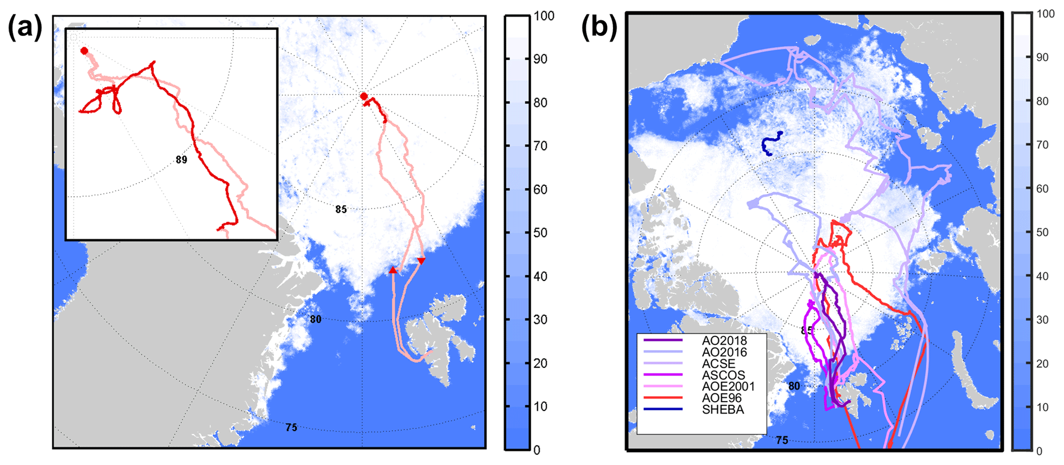
Figure 1(a) AO2018 cruise track (pink) with the ice drift track (14 August–14 September 2018, red and inset). The measurement stations within the marginal ice zone are marked by ▴ (inbound, 2 August 2018) and ▾ (outbound, 20 September 2018), and the “North Pole” station by • (12 August 2018). Colour gradient shows ice concentration (%) for 1 September 2018, obtained from the University of Bremen satellite sea ice product (http://seaice.uni-bremen.de, last access: 4 January 2021, Spreen et al., 2008). (b) Cruise tracks of previous campaigns conducted in the Central Arctic ocean with same ice concentration as shown in panel (a).
Table 1Overview of cruise dates for AO2018 and the previous campaigns shown in Fig. 1.

AO2018 took place on the Swedish icebreaker Oden, between 1 August and 21 September 2018, departing from and returning to Longyearbyen. The expedition track and principal measurement stations are shown in Fig. 1a. Oden entered the sea ice on 2 August, conducting a 24 h measurement within the marginal ice zone (MIZ) (82.1547∘ N, 9.9695∘ E, from 23:00 UTC) before making its way toward the North Pole. Measurements were undertaken at the closest point to the pole achievable (89.8932∘ N, 38.0423∘ E). At about 20:00 UTC on 13 August the Oden moored to a stable large ice floe on which to undertake measurements and drifted with it until 21:00 UTC on 14 September. A final 24 h measurement period was undertaken on 20 September within the MIZ (82.2833∘ N, 19.8333∘ E) before leaving the ice.
The meteorological component of AO2018 combined two projects: Microbiology-Ocean-Cloud Coupling in the High Arctic (MOCCHA)1 and Arctic Climate Across Scales (ACAS)2. The projects shared many measurements and operated jointly during the expedition.
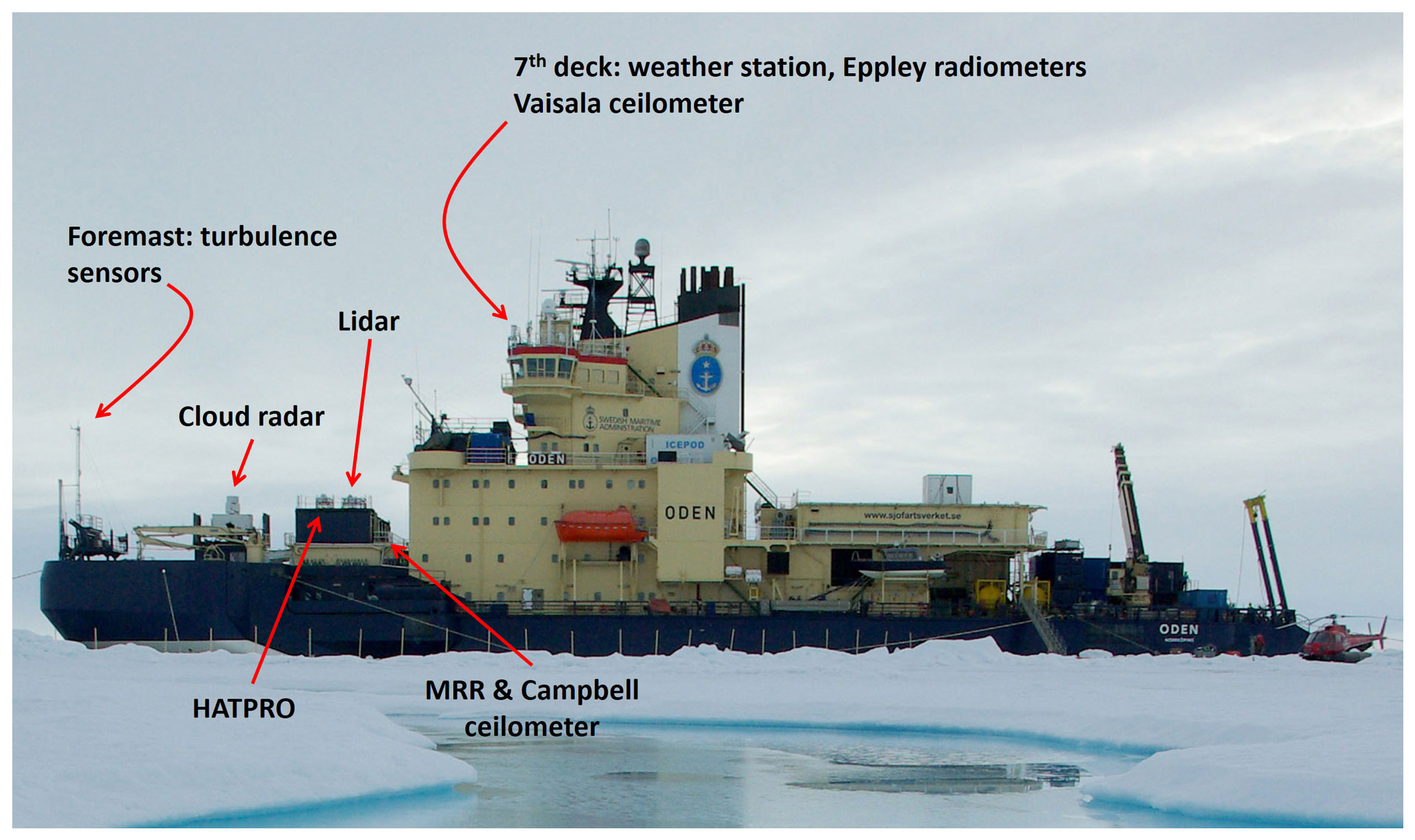
An overview of the measurement systems is given in Table 2 and shown in Fig. 2. A suite of atmospheric remote sensing instruments operated almost continuously throughout the expedition, providing a mobile Cloudnet (Illingworth et al., 2007) site. A METEK MIRA-35 scanning Doppler cloud radar was installed on the roof of a container on Oden's foredeck; a HALO Photonics StreamLine scanning micro-pulsed Doppler lidar (Pearson et al., 2009) was installed within a motion-stabilised table (Achtert et al., 2015) on top of a container above the foredeck laboratory. A Radiometer Physics HATPRO scanning microwave radiometer was installed alongside the lidar. Radiosondes (Vaisala RS92) were launched from the ship's helipad every 6 h (00:00, 06:00, 12:00, 18:00 UTC); data from these were shared globally in near-real time over the Global Telecommunication System.
The measurements from these instruments allow a detailed characterisation of clouds using the Cloudnet algorithm. Cloudnet averages the data to a common grid at the cloud radar resolution and provides an objective hydrometeor target classification. Further products are derived on the basis of the hydrometeor target classification and the available measurements, including cloud occurrence, top and base height, cloud thickness, cloud phase, liquid water content, ice water content, and the effective radius of cloud droplets and ice crystals. Details of the preliminary data processing steps required prior to running the Cloudnet retrieval and further information on the product retrievals are documented in Achtert et al. (2020).
Additional remote sensing measurements were made by a Campbell CS135 laser ceilometer and a METEK MRR2 Micro Rain Radar, both installed above the foredeck laboratory. A Particle Metrics Forward Scattering Spectrometer Probe (FSSP-100) was installed above the container laboratories on deck 4 to measure the drop size distributions of fog. It was mounted on a motorised rotator with a control system that monitored the local wind direction and kept the FSSP oriented into wind.
On the seventh deck, approximately 25 m above the surface, a second ceilometer (Vaisala CL31) was installed, along with a weather station measuring pressure (Vaisala PTU300), temperature and relative humidity (RH) (aspirated Rotronic MP101), wind speed and direction (heated Gill WindSonic M), and broadband downwelling solar and infrared radiation (Eppley PSP and PIR mounted on gimbals). A Heitronics KT15-II infrared temperature sensor measured the surface temperature. A present weather sensor (Vaisala PWD22) measured visibility, precipitation type, precipitation intensity, and precipitation amount.
Table 2Overview of meteorological instruments. All heights for instrumentation on Oden are given relative to the waterline.
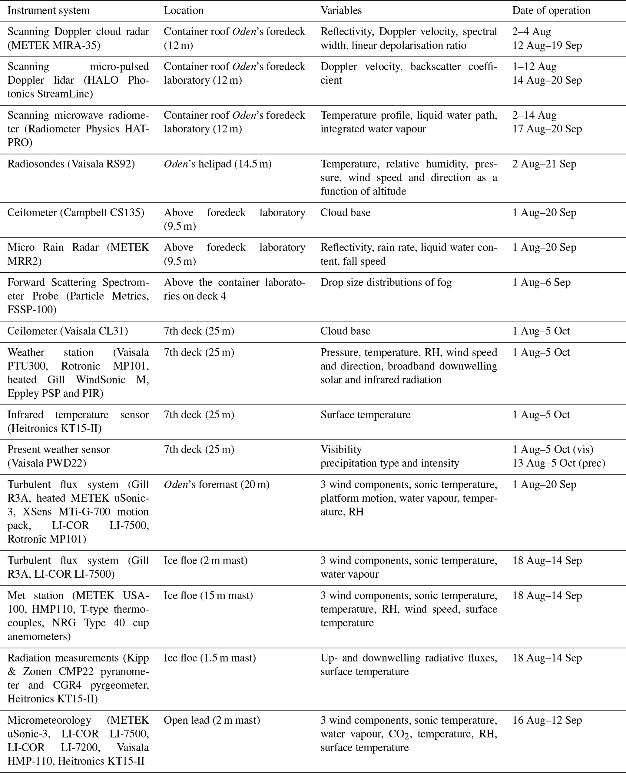
A turbulent flux system was installed on the foremast immediately above the bow at a height of 20 m above the surface. This consisted of a sonic anemometer (heated METEK uSonic-3), with an XSens MTi-G-700 motion pack to measure platform motion, a LI-COR LI-7500 infrared gas analyser to measure water vapour, and an aspirated Rotronic MP101 to provide a reference temperature and RH at the top of the foremast. Wind measurements are corrected for platform motion and for flow distortion around the ship (Prytherch et al., 2015, 2017). Flux estimates were calculated via eddy covariance over 30 min averaging intervals, and standard statistical quality control tests for skewness, kurtosis (Vickers and Mahrt, 1997), and stationarity (Foken and Wichura, 1996) were applied to flag unreliable estimates. Periods with flow from aft (wind directions more than 120∘ from the bow) are heavily contaminated by turbulence generated by the ship's superstructure and were excluded. Such periods are very few because the ship was re-oriented into the wind on a regular basis to maintain clean sampling for the extensive aerosol measurements being made by other groups on board. Ship-based instrument systems were operated nearly continuously throughout the whole expedition (Table 2). The scanning Doppler cloud radar could not be operated during heavy ice breaking between 5 and 13 August due to excessive vibration. The radar performed one range-height indicator (RHI) scan every 30 min and was operated in vertical stare mode the rest of the time. On the transit out of the ice it operated in vertical stare mode only. Precipitation data from the present weather sensor are only available from 13 August onwards. The rest of the data sets only have smaller data gaps.
During the 4-week drift, additional measurement systems were installed on the ice floe. A 15 m mast was erected about 300 m from the ship with a heated sonic anemometer (METEK USA-100) at the top of the mast (15.55 m) and a Vaisala HMP-110 probe in an aspirated radiation shield just below the top of the mast, to measure temperature and RH. Four more aspirated shields with T-type thermocouples were mounted at approximately logarithmically spaced heights (0.80, 1.55, 3.05, 8.80 m) to measure the near-surface temperature profile. A final thermocouple was buried at the ice–snow interface. NRG Type 40 cup anemometers were mounted at five levels (0.65, 1.45, 2.86, 6.65, 13.25 m) to provide a near-surface wind-speed profile. A second 2 m tall mast was located nearby with a Gill R3A sonic anemometer and a LI-COR LI-7500 gas analyser to make direct water vapour flux measurements. About 50 m from the main mast, pairs of solar and infrared radiometers (Kipp & Zonen CMP22 pyranometer and CGR4 pyrgeometer) were installed to measure up- and downwelling radiative fluxes over an undisturbed snow surface at 1.5 m height. Another Heitronics KT15-II measured the surface temperature immediately below the radiometers.
A second site was located at the edge of an open lead, approximately 1.5 km from the ship. A 2 m mast was instrumented with a METEK uSonic-3 sonic anemometer and two LI-COR infrared gas analysers: an open-path LI-7500 was used for water vapour measurements, from which the latent heat flux was calculated, and a closed-path LI-7200 was used to make CO2 flux estimates. An aspirated Vaisala HMP-110 measured air temperature and RH, and a Heitronics KT15-II infrared temperature sensor measured the skin temperature of the open lead surface.

Figure 3Contour plots of (a) mean sea-level pressure in hectopascals (hPa) and its (b) climatological anomaly (1981–2010) for the AO2018 measurement period. Image provided by the NOAA/ESRL Physical Sciences Division, Boulder, Colorado, USA, from their website at http://www.esrl.noaa.gov/psd/ (last access: 4 January 2021). Based on NCEP Reanalysis data (Kalnay et al., 1996).
Synoptic-scale atmospheric conditions exhibit large annual and interannual variability. To put the relatively short observation period from AO2018 in a larger context, prevailing conditions for 2018 are compared to climatology using NCEP Reanalysis data. Figure 3 shows mean sea-level pressure (MSLP) and its anomaly from the 1981–2010 climatology for the time of the measurement campaign. There are two separate high-pressure areas, one over Greenland and one stretching from the Beaufort Sea over the East Siberian Sea to the Laptev Sea. Low pressure is centred over the Canadian Arctic Archipelago to the west and over the Barents Sea to the east, with the area around the North Pole, where the expedition took place, between these two low-pressure centres. The pressure pattern is anomalous compared to the 1981–2010 climatology, with a negative anomaly of more than 5 hPa over the Canadian Arctic Archipelago, 4 hPa over the Barents Sea, and around 1 hPa over the measurement location. The positive anomaly over the Beaufort and East Siberian seas was weaker than the negative anomalies, only 1–2 hPa.
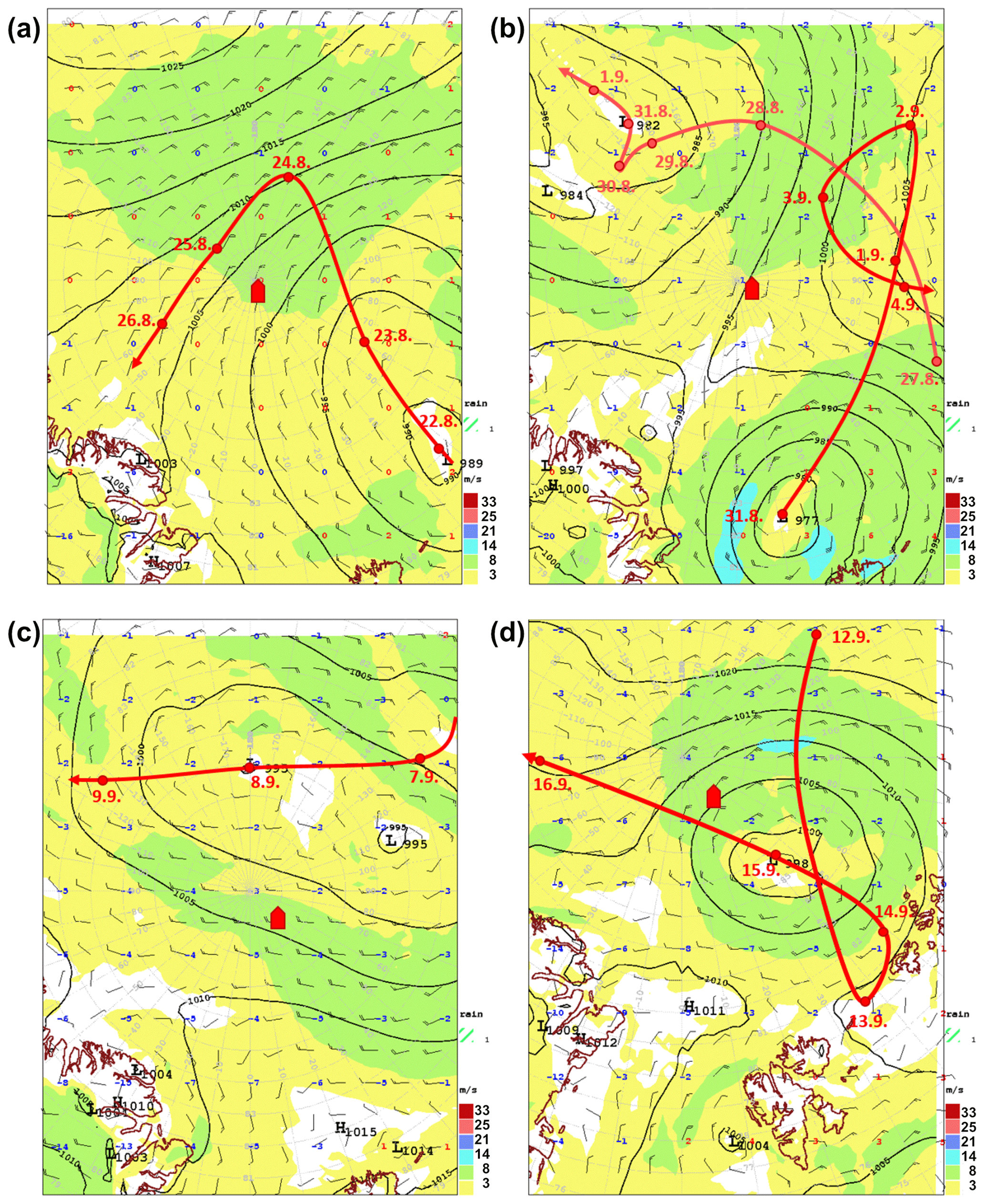
Figure 4ECMWF charts showing sea-level pressure, near-surface wind, and precipitation at 00:00 UTC for 4 d: (a) 22, (b) 31 August, (c) 8, and (d) 15 September 2018. The figures also show storm tracks for the major low-pressure systems passing through the area with their low-pressure centres at 00:00 UTC on the respective day. The approximate location of the icebreaker Oden is marked by the red arrow.
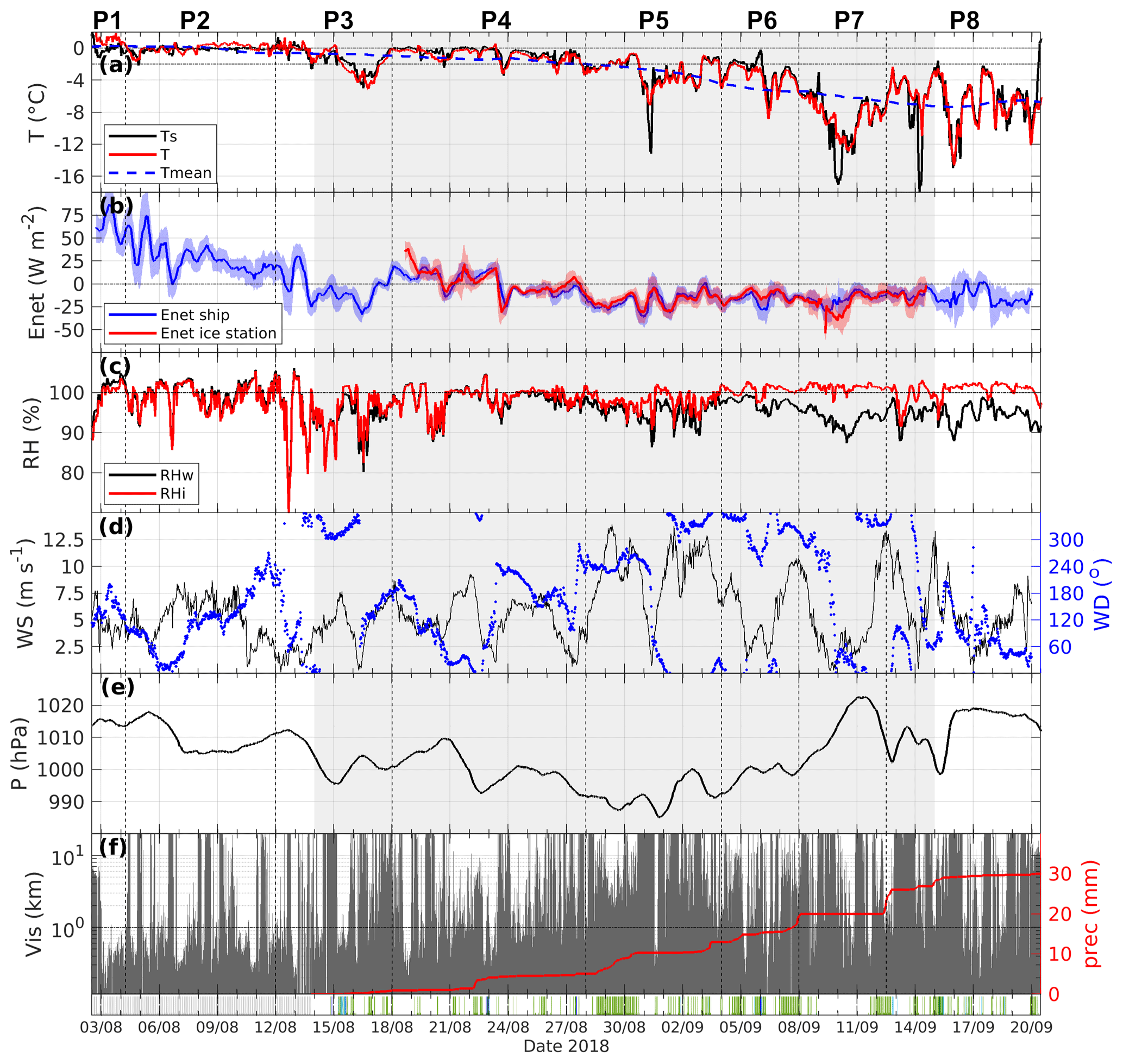
Figure 5Time series of (a) surface temperature, near-surface air temperature, and 14 d running mean of near-surface temperature; (b) 12 h running mean of surface energy ± 1 standard deviation (shaded area); (c) RHw and RHi; (d) wind speed and wind direction; (e) air pressure; (f) visibility, accumulated precipitation and precipitation type. Data in panels (a), (c), (e), and (f) are from instruments installed on the seventh deck of the ship. Turbulent fluxes for calculation of panel (b) and wind measurements are from the foremast of the ship. Net radiation for calculation of (b) is from measurements on the ship (blue line) and the station on the ice floe (red line). Vertical dashed lines mark the identified key periods P1 to P8, and the grey shaded area represents the drift period. The precipitation type in panel (f) is colour coded. Grey is missing data, blue is drizzle and rain, and green is snow and ice.
The synoptic-scale weather development resulting from this large-scale setting is illustrated in Fig. 4. ECMWF surface-pressure, precipitation, and 10 m wind charts are shown at weekly intervals through the ice drift, including the tracks for the five most significant low-pressure systems. The cyclonic activity seen here started in the middle of August and lasted until the end of the campaign in September. Earlier, the synoptic activity was weaker, with some weaker low-pressure systems influencing the AO2018 track in addition to some high-pressure influence (Fig. 5e). The first strong low-pressure system developed over the Barents Sea on 22 August (Fig. 4a), moving anticlockwise around the pole, bringing precipitation and enhanced wind speeds towards the location of the AO2018 ice drift (Fig. 5d, f). Two more low-pressure systems developed on 27 and on 31 August (Fig. 4b). One developed over the Kara Sea, also moving anticlockwise around the pole and dissipating in the Canada Basin, whereas the other developed between Greenland and Svalbard, first moving eastwards and then turning around towards the Kara Sea. These systems also affected the AO2018 ice drift, bringing precipitation and strong winds (Fig. 5d, f). The fourth low-pressure system moved from the Laptev Sea on 7 September (Fig. 4c) towards the Beaufort Sea, and the last system developed over the East Siberian Sea on 12 September (Fig. 4d), moved towards Svalbard, and then moved towards the Canadian Basin.
4.1 Near-surface conditions
Measurements of near-surface conditions undertaken on board the ship on the seventh deck (approximately 25 m a.m.s.l.) and at the foremast are shown in Fig. 5. The net surface energy was calculated from radiation measurements on board the ship and on the ice floe together with turbulent flux measurements from the foremast. Upward radiative fluxes were only directly measured on the ice. For the ship-based radiation measurements, the upwelling long-wave radiation was calculated using blackbody radiation from the KT15 surface temperature measurements, assuming an emissivity of unity. The short-wave upwelling radiation was calculated using 3-hourly albedo estimates made from surface images of the surrounding of the ship. All fluxes are defined positive if they are directed towards the surface. Hence, a positive net surface energy flux represents energy input into the surface.
Wind speeds measured at the foremast varied between 0 and 13 m s−1 (Fig. 5d). The strong variability was caused by the passage of the aforementioned low-pressure systems. The time series of near-surface temperature shows the transition between melt and freeze season (Fig. 5a). From the beginning of the campaign until 28 August, surface and air temperatures were mostly between 0 and −2 ∘C with brief cooler periods of 1 to 2 d, usually with occurrences of clear skies. This is representative of the sea ice melt season when net positive surface energy acts to melt snow and ice but cannot warm the surface above the freezing point whilst the melting ice and snow remains. From 23 August onward temperatures gradually cooled and with another sudden drop on 28 August stayed below 0 ∘C, mostly below −2 ∘C, with a minimum surface temperature of −18 ∘C, also in a cloud-free period. An often-used definition for the onset of the freeze-up is the time when the running-mean near-surface air temperature falls below a certain threshold (Colony et al. 1992, Rigor et al., 2000; Tjernström et al., 2012). Here we follow Tjernström et al. (2012) using a threshold of −2 ∘C, which puts the start of the freeze-up at 28 August (Fig. 5a). The 5 d before 28 August show a slow transition between melt and freeze conditions, with the surface undergoing multiple freezing and melting cycles. The freeze onset can also be defined using the net surface energy. A surplus in surface energy melts the ice, and negative values indicate freezing. As can be seen in Fig. 5b, net surface energy drops below 0 W m−2 on around 23 August but recovers briefly to above 0 W m−2 on 27 August. From 28 August onwards it stays below 0 W m−2, coinciding with the freeze onset defined previously. Therefore, we will refer to the measurement period before 28 August as the melt period and afterwards as the freeze-up period.
The near-surface atmosphere was very moist throughout the campaign. RH with respect to water (RHw) was mostly between 90 and 100 % (Fig. 5c). Only the beginning of the expedition until 17 August RHw was more variable, ranging between 80 and 100 %. RH with respect to ice (RHi) was in the same range until the freeze-up. After 28 August RHi continued to be close to 100 % with a slight supersaturation, consistent with Andreas et al. (2002), while RHw declined from 4 September onwards (Fig. 5c). This change in near-surface relative humidity is also reflected in the visibility (Fig. 5f). The visibility is more often limited, often <1 km (fog), during the melt. When the near-surface air becomes saturated with respect to ice and more precipitation falls as snow, the visibility is higher, since fog droplets tend to evaporate or deposit on the surface. Over 93 % of the measured precipitation fell as snow or ice; only during a few events was freezing drizzle (4.6 %) or freezing rain (1.8 %) detected (Fig. 5f). Liquid precipitation was only detected 1.3 % of the time as drizzle or rain.
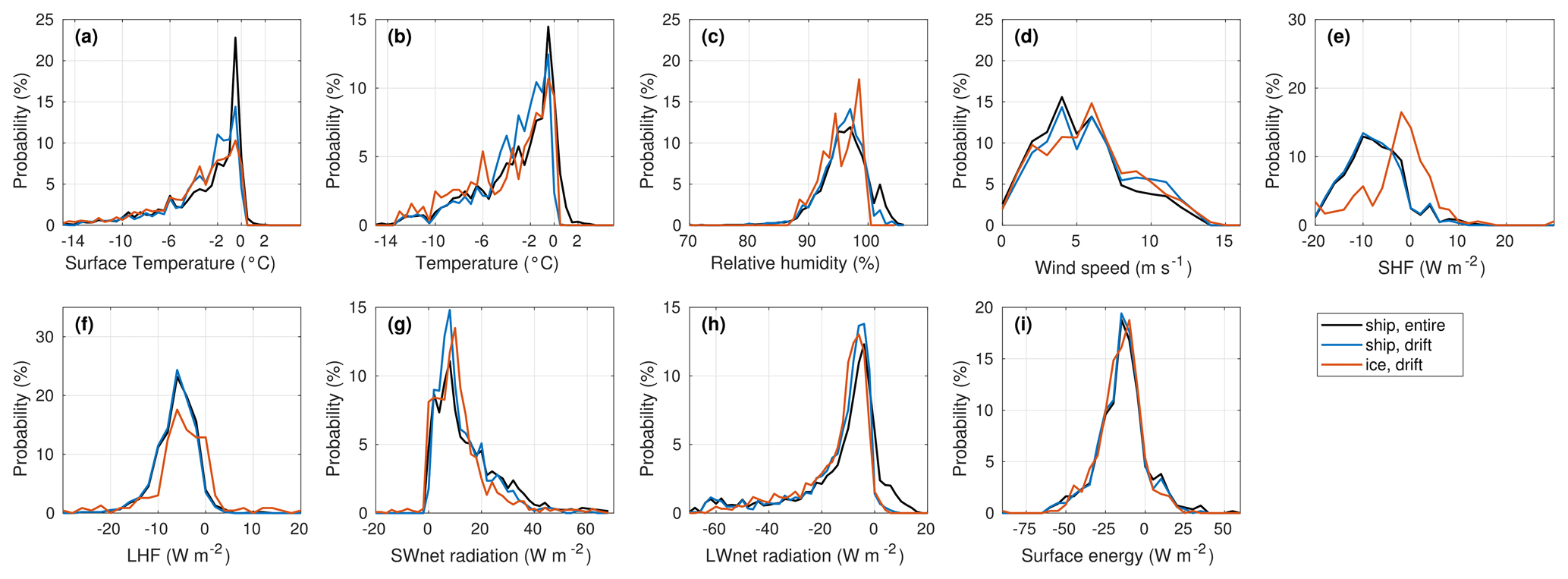
Figure 6Probability distributions of (a) surface temperature, (b) near-surface air temperature, (c) RHw, (d) wind speed, (e) sensible heat flux, (f) latent heat flux, (g) short-wave net radiation, (h) long-wave net radiation, and (i) surface energy. Data are from measurements on board the ship for the whole measurement period (black lines), for the ice drift period only (blue line), and from the measurement station on the ice floe (orange line).
The probability distributions of ice surface temperatures peak in the range between −1.8 and 0.0 ∘C (Fig. 6a), the freezing points of seawater and freshwater, respectively, representing the conditions during the melt period. A secondary peak at −3 ∘C and the long tails towards colder temperatures represent the freeze-up. For near-surface air temperature the distributions also peak between −1.8 and 0.0 ∘C (Fig. 6b), which reflects the strong surface control on near-surface air temperature during the melt seasons and the colder temperatures mostly reflect the freeze period. The slight differences between the ship and the ice station measurements result from data gaps in the ice station time series; removing the additional ship data and creating a like-for-like comparison removes almost all the difference. As the near-surface atmosphere was very moist, the distribution for the RHw measurements peaks between 95 and 98 % for the ship-based measurements (Fig. 6c). The measurements from the ice station have peaks at 94 and 99 %. The probability distributions for the wind speeds peak at 4.5 m s−1 for the ship measurements and 6.5 m s−1 for the ice station (Fig. 6d). The differences again come from data gaps in the ice station time series. All distributions have a tail of higher speeds, reaching 16.0 m s−1. For the ice drift period both measurement sites show a higher probability of wind speeds above 9.0 m s−1, reflecting the stronger synoptic activity during the ice drift period.
4.2 Surface fluxes
The turbulent fluxes were small as expected. The sensible heat flux calculated from the ship measurements peaked between −10 and 0 W m−2 with tails for both the whole campaign and for the ice drift period only towards −20 and 10 W m−2 (Fig. 6e). The distribution for the ice station peaked at −1 W m−2 with tails towards −20 and 10 W m−2. The latent heat flux peaked at −5 W m−2 for the ice and ship station, with a wider tail towards negative values around −20 W m−2 (Fig. 6f). The distributions of net short-wave radiation peak around 9 W m−2 with a long tail towards 70 W m−2 for both the whole measurement period and the ice drift (Fig. 6g). Net long-wave radiation peaks at around −5 W m−2 with a similarly long tail towards −70 W m−2 (Fig. 6h). The total net surface energy distributions are very similar for the ice and ship measurements, peaking at −10 and −15 W m−2, respectively (Fig. 6i). All distributions have a tail towards −60 W m−2 and shorter tail towards positive values.
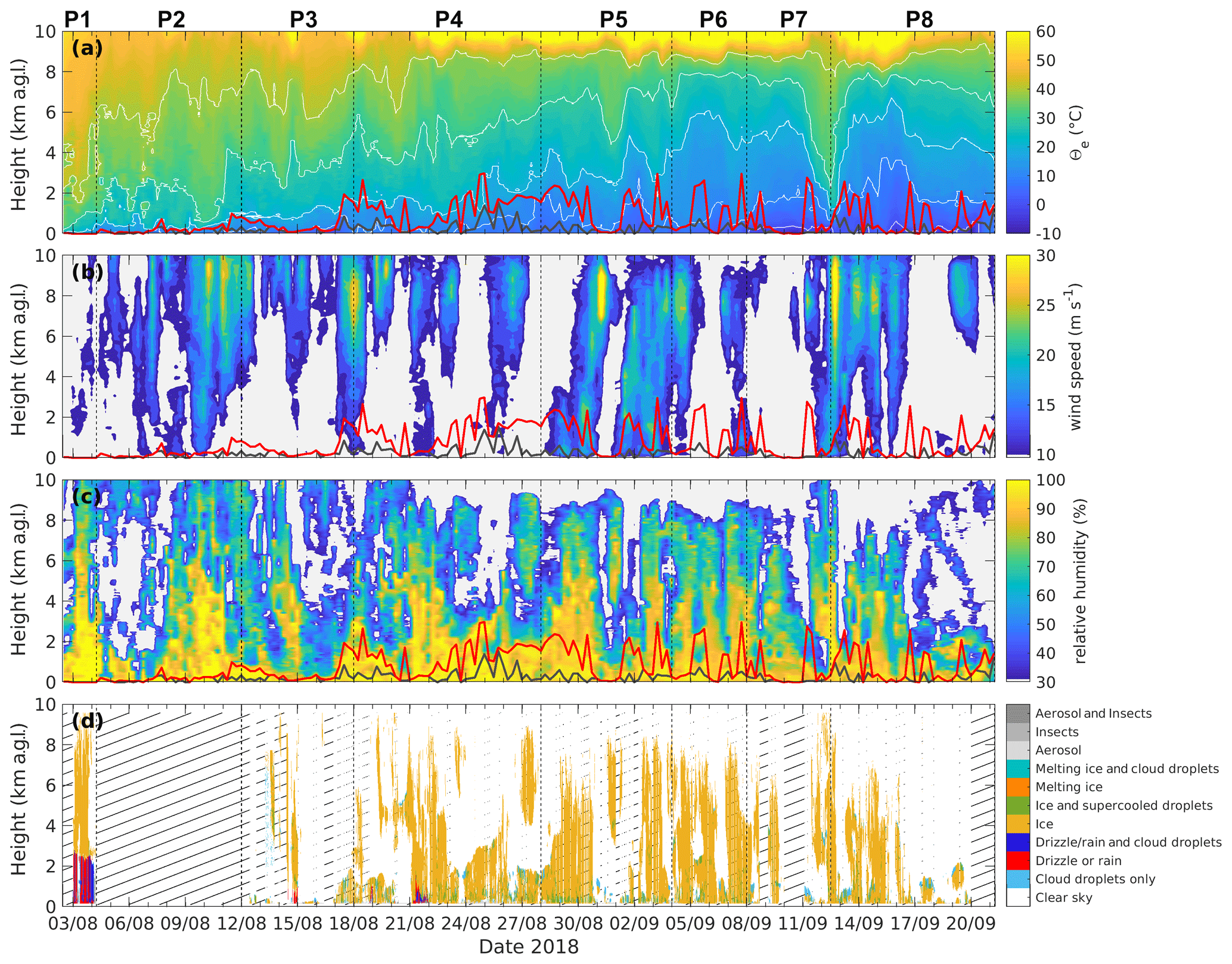
Figure 7Contour plots of (a) equivalent potential temperature, (b) wind speed, (c) RHw measured by radiosondes, and (d) cloud target classification from the Cloudnet algorithm. The red lines in panels (a)–(c) show the main inversion base height, and the grey lines the surface mixed layer depth identified from radiosonde data. Dashed vertical lines mark the identified key periods. Striped grey areas in panel (d) represent times of missing data.
4.3 Vertical structure
Time–height cross sections of equivalent potential temperature, wind speed, and RHw measured by radiosondes give an overview of the vertical structure of the atmosphere during the expedition (Fig. 7a–c). Additionally, cloud target classification from the Cloudnet algorithm gives an overview of cloud cover and cloud phase for the same time period (Fig. 7d). The thermal structure shows a gradual cooling and reduction of stability over time. Several frontal systems affected the measurement area during the campaign. These systems were associated with deep frontal clouds and strong winds throughout the whole troposphere. Between those high-wind periods, wind speeds were low not only within the surface mixed layer (SML) but also aloft. RHw was high within the SML. Aloft, RHw was very variable. Within frontal systems, RHw was high throughout the whole vertical column, whereas it dropped to below 30 % above the SML on several other occasions. RHi (not shown) shows a gradual descent in altitude of the saturation level over time, from around 2 to 3 km in mid-August to close to the surface in early September.

Figure 8Probability of (a) equivalent potential temperature and (b) RHw as a function of altitude. Note that the probability is calculated for each height; hence, for each layer the probability sums to 100 %. The solid red line shows the mean, and the dashed red line the median profile.
The probability distributions of equivalent potential temperature and RHw as a function of altitude show that there are two predominant structures occurring in the vertical thermodynamic profiles (Fig. 8): one with a well-mixed deep layer up to ∼1.5 km and the other with a shallower well-mixed layer reaching 400 to 500 m. Both are capped by a temperature inversion. The well-mixed near-surface layers appeared preferentially at an equivalent potential temperature between 8.0 and 10.0 or 4.5 ∘C and were very moist with relative humidity between 90 and 100 %. The RHw distribution shows a very moist layer with humidity above 90 % up to about 800–1000 m.
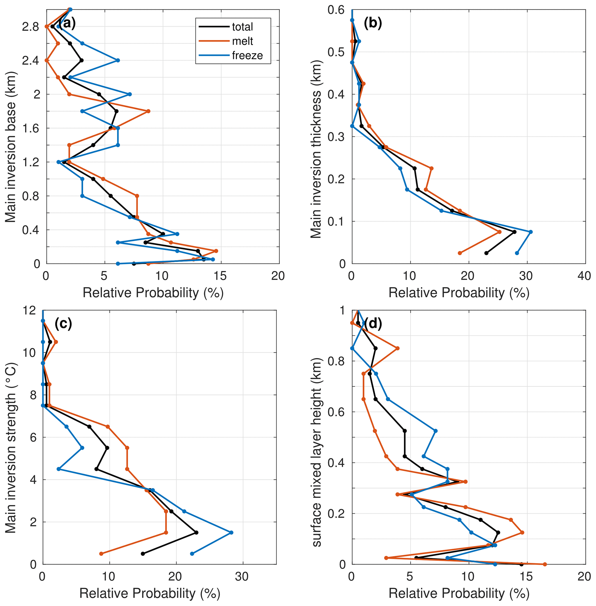
Figure 9Probability distributions of (a) main capping inversion base, (b) main capping inversion thickness, (c) main capping inversion strength, and (d) SML height, as detected from radiosonde data. Results are shown for the entire campaign (black lines), for the melt period before 28 August (orange lines), and for the freeze period of all data after 28 August (blue lines).
The characteristics of the main temperature capping inversion are shown in Fig. 9. To identify the main capping inversion from the radiosonde profiles, an objective algorithm is applied to the temperature and equivalent potential temperature profiles in a decision-tree-like process mostly following Tjernström and Graversen (2009). To summarise, all layers with a positive temperature gradient deeper than 20 m within the lowest 3 km are identified, and layers separated by less than 100 m are merged. The layer with the strongest gradient is considered the main inversion. If no temperature inversion can be identified, the strongest stable layer within the lowest 3 km that is at least 20 m deep and 0.1 K strong is identified using the equivalent potential temperature profiles and used as a proxy for the main inversion. The main inversion base is used as a proxy for the BL height. If there are weaker inversions below the main inversion, the lowest inversion base is considered to be the height of SML and the rest of the BL is considered to be decoupled from surface-induced turbulence. In a similar decision-tree process to that for the main inversion, the strongest stable layer below the main inversion was considered as the SML when no weaker temperature inversion could be found. In addition to the radiosonde data, surface temperature measurements from the KT15 on board the ship were used to identify surface inversions. If the temperature was monotonically increasing from the surface to the lowest measurement heights of the radiosonde (30 m), it was classified as a surface inversion. In these stable conditions surface processes are also decoupled from the rest of the BL.
The analysis for all available radiosondes revealed that the BL was coupled for 41.0 % of the time and decoupled for 59.0 % of the time. From those 59.0 % of decoupled cases, 13.5 % were decoupled by a surface inversion, and the other 45.5 % by a weaker inversion below the main capping inversion. Surface inversions occurred preliminary during the calm conditions, at the beginning of the campaign (Fig. 7). The probability distributions of the capping inversion and SML characteristics are shown in Fig. 9. The main capping inversion base height shows a bimodality with a maximum below 400 m and another one around 1500 m. High main capping inversions are mostly connected to the passage of frontal systems. The inversions were 50 to 300 m thick, and the inversion strength shows a broad distribution of 1.0 to 8.0 K, with a maximum at around 1.5 K. The SML was mostly between 50 and 400 m deep.
4.4 Cloud characteristics
Cloud characteristics and cloud phase are determined on a profile-by-profile basis using the Cloudnet target classification (Illingworth et al., 2007) with a temporal resolution of 30 s following Achtert et al. (2020). For the entire measurement period 94 102 profiles are available. From these profiles, only 4 % detected no clouds, while 41 % had a single cloud layer, and 54 % multiple cloud layers. Profiles of cloud fraction per volume (Brooks et al., 2005) have been obtained using time–height sections of 30 min and 90 m height. As shown by Achtert et al. (2020), the target classification reveals an unrealistically high occurrence of the targets aerosol, aerosol and insects, and insects during periods that were actually dominated by fog. Hence, we follow their approach and re-classify the targets for these categories as fog during periods with visibility <1 km. Note, however, that the radar's lowest range gate is at 156 m, and consequently many of the shallower fog episodes were missed by the radar. For AO2018 visibility data show that 49 % of the fog occasions were too shallow to be detected by Cloudnet, so very low level liquid clouds are likely underestimated.
Fog depths could still be calculated using radar RHI scans. Radar reflectivity was averaged between 150 and 1000 m away from the radar to obtain mean vertical profiles of radar reflectivity. The fog layer top height was defined as the strongest negative vertical reflectivity gradient in the lowest 500 m. If there were several cloud layers in the first 500 m, the strongest gradient in the lowest layer was used for the fog depth. As radar reflectivity is proportional to the drop diameter to the power of 6, light precipitation or drizzle can be expected to influence the results for higher reflectivity. Hence, the Micro Rain Radar data were used to reject all detected fog heights during precipitation events. Fog, defined as visibility <1 km, was detected approximately 21 % of the time during AO2018 (Fig. 10a). The probability distribution of the fog depths is shown in Fig. 10b. The most common fog depth was between 120 and 150 m, below the lowest range gate of the radar, with a median of 205 m and a tail extending just above 500 m.
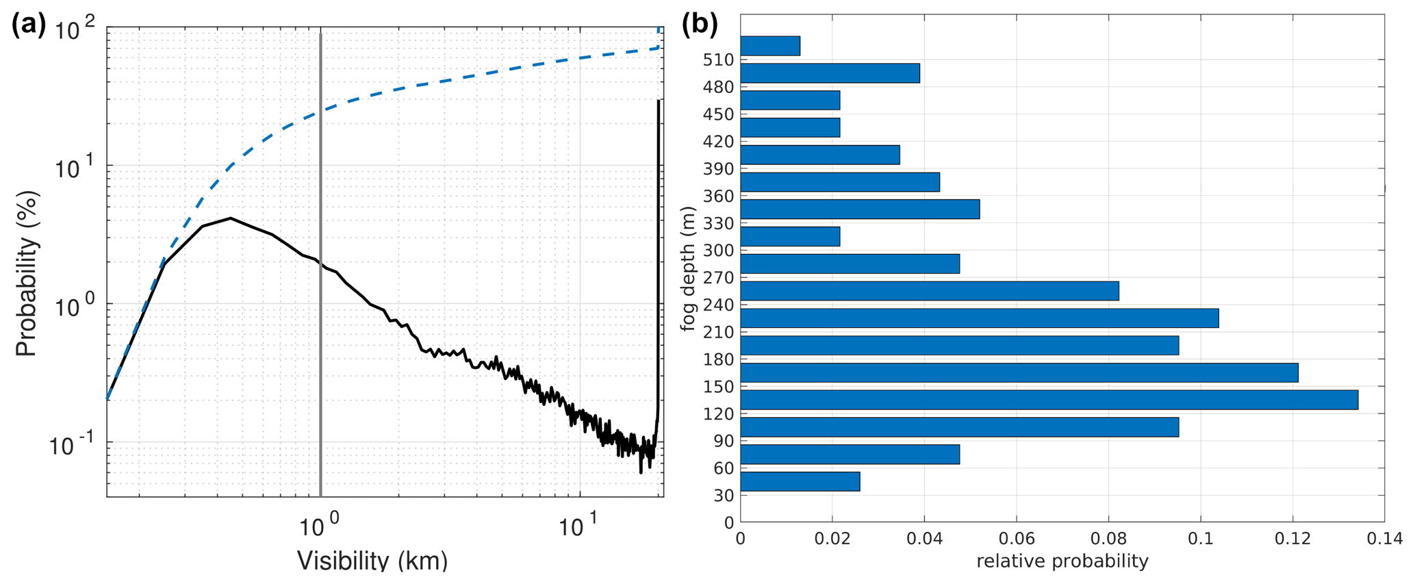
Figure 10(a) Probability distribution and accumulated probability (dashed blue line) of visibility. The black vertical line marks 1 km visibility. (b) Probability distribution of fog depths detected using radar RHI scans.
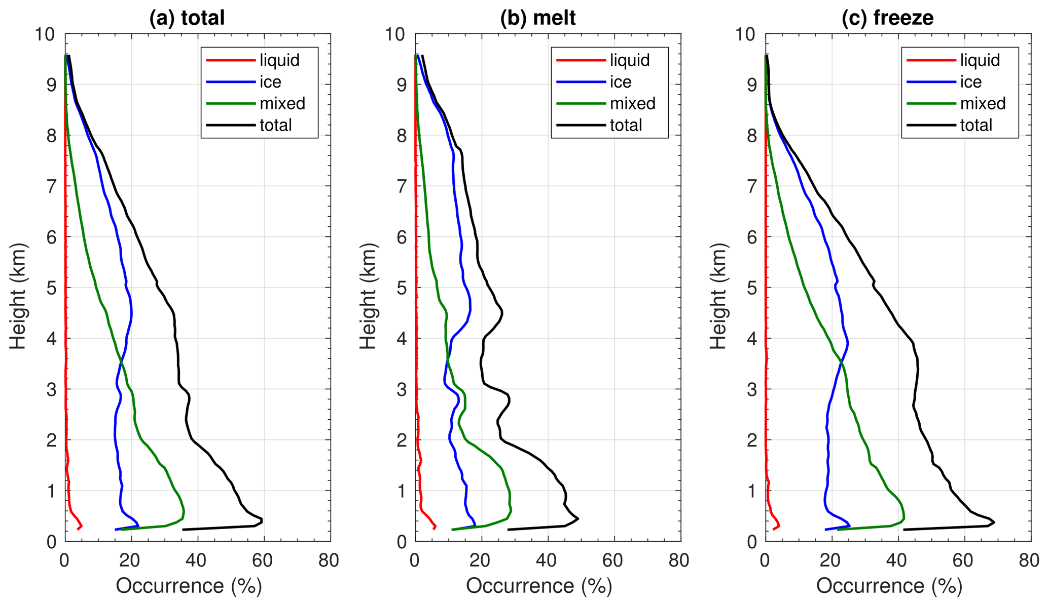
Figure 11Mean cloud occurrence per volume for different cloud types, obtained from the Cloudnet target classification product: mean profiles (a) for all available Cloudnet data, (b) for the melt period, and (c) for the freeze period.
Calculated cloud occurrence probability distributions as a function of height are shown for the entire campaign, the melt period, and the freeze period in Fig. 11. Cloud fraction was largest below 1 km for the entire campaign and separately for both melt and freeze-up periods. This is reflected by a maximum cloud fraction below 500 m of approximately 65 % for the entire campaign, 49 % for the melt period, and 69 % during freeze-up. A secondary maximum appears between 2.5 and 3.0 km for the total and for the melt period distribution. A third maximum appears for the melt period at around 4.5 km. During the freeze-up period the secondary maximum was higher, at 3.0 to 4.0 km. These secondary maxima reflect the frequent occurrence of multiple cloud layers during AO2018. Mixed-phase clouds were the most abundant cloud type occurring below 3.5 km, and some mixed-phase clouds were observed up to a height of 8 to 9 km. Above these levels ice clouds dominated. Some mixed-phase clouds might be underestimated in multi-layer cloud situation if the lidar signal gets fully attenuated in the lower layers. Liquid-only clouds were rarely observed in either season, even for the low altitudes. Note, however, that liquid water clouds occurring below the lowest radar range gate (fog) are not included here.
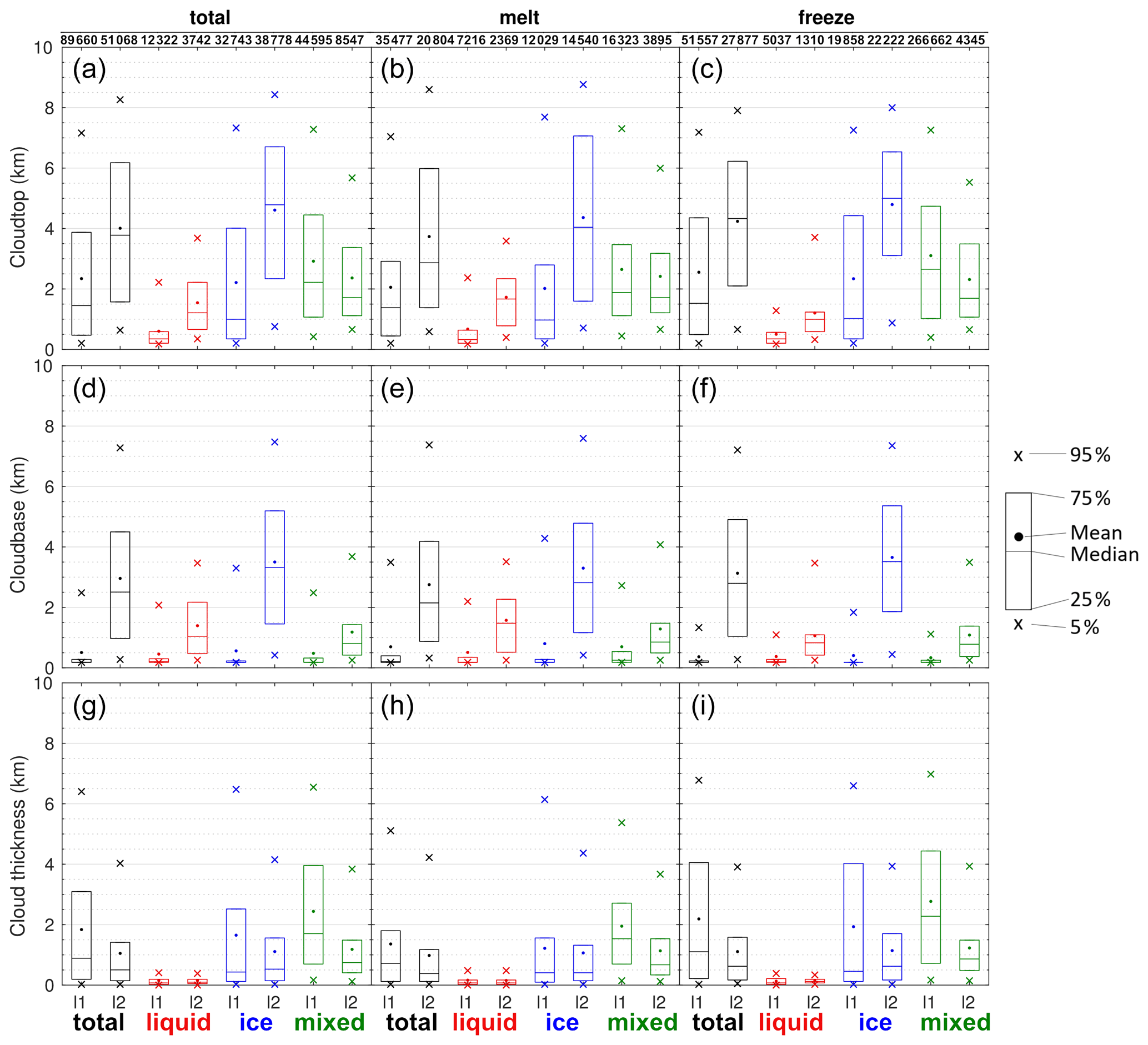
Figure 12Statistical overview of cloud top height (a–c), cloud base height (d–f), and geometrical thickness (g–i) for the entire AO2018 campaign (a, d, g) as well as for melt (b, e, h) and freeze (g, h, i) conditions. The colours indicate different cloud types. Results for the lowest two cloud layers (l1 and l2) are shown. The top row shows the number of profiles used for each boxplot.
Statistics of cloud top, base, and thickness are shown in Fig. 12 for the lowest two cloud layers separated by cloud phase. A limitation of the Cloudnet approach is that there is no distinction between falling ice particles and cloud ice. Hence, ice precipitation extends the apparent cloud boundaries. Furthermore, results flagged as one cloud might actually contain two cloud layers with ice precipitating from the upper clouds into the lower. This might be the case for the thicker ice and mixed-phase clouds in particular. Based on an analysis of cloud radar Doppler spectrographs from ASCOS, Sotiropolou et al. (2014) suggested that a mixed-phase cloud depth of over 700 m might be considered two cloud layers.
Vassel et al. (2019) provide a method of detecting possible seeding events combining radiosonde and radar data. In step 1, ice-supersaturated and ice-subsaturated layers are identified using relative humidity data from radiosonde profiles. The sublimation of an ice crystal through the subsaturated layer is calculated assuming an initial size of 400 µm but is also calculated for 100 and 200 µm. If the ice crystal is not fully sublimated when reaching a lower supersaturated layer, potential seeding is taking place. In a second step the results are cross-checked for actual cloud occurrence using radar reflectivity. Radiosonde data were available every 6 h, and radar data were only available during the drift period. Hence, the method of Vassel et al. (2019) was applied 6-hourly between 13 August and 14 September, resulting in 117 analysed profiles. Radar data were used for 30 min either side of the radiosonde launch. Twelve per cent of the data show no cloud occurrence. Results for single-layer and multi-layer clouds vary with assumed ice crystal size. Single-layer clouds occur in 32 % (r=100 µm: 50 %; r=200 µm: 38 %) of the analysed profiles for an assumed size of 400 µm. Non-seeding multi-layer clouds occur in 13 % (r=100 µm: 8 %; r=200 µm: 11 %), seeding multi-layer clouds in 37 % (r=100 µm: 18 %, r=200 µm: 30 %), and profiles with both seeding and non-seeding layers in 11 % (r=100 µm: 7 %; r=200 µm: 9 %) of the profiles.
These results strengthen our hypothesis of multi-layer seeding clouds, and these limitations should be kept in mind for comparisons with other observational results not obtained with the Cloudnet algorithm. For a comparison with model results, this might not cause problems, as some models treat falling ice particles the same way as the Cloudnet algorithm or ice precipitation can be included for statistics.
For the first cloud layer, mixed-phase clouds were detected in 47 and 52 % of the profiles during melt and freeze, respectively. During melt another 19 % of the lowest clouds were identified as liquid clouds, and 34 % as ice clouds. For the freeze period only 10 % were liquid clouds, and 38 % were ice clouds. The results for the lowest cloud layer show that all of the clouds have very low cloud bases, with median cloud bases at 180 to 200 m; including the lowest clouds below the radar's lowest range gate, this is probably even lower. Liquid clouds are by far the thinnest clouds, with a median thickness of 72 m, while ice clouds have a median thickness of around 400 to 450 m for both seasons. Their vertical extent is quite variable as indicated by the much higher mean cloud thickness and the extent of the 75th and 95th percentile. However, these results also contain precipitating ice clouds, where ice precipitation might extend the actual cloud boundaries. First-layer mixed-phase clouds are considerably thicker than ice clouds, with a median thickness of 1500 and 2280 m for the melt and freeze periods, respectively.
In the case of multiple cloud layers, 71 % of the second-layer clouds were ice clouds during melt, and 80 % during the freeze period. Second-layer ice clouds have a much higher cloud base than second-layer mixed and liquid clouds, with a median cloud base height of around 2800 m during melt and 3500 m during freeze compared with 800 m for mixed-phase clouds in both seasons and 1500 and 800 m for liquid clouds during melt and freeze, respectively. The thickness of liquid second-layer clouds is, as for the first layer, very thin, with a median value of 72 m during melt and 120 m during the freeze period. Second-layer ice clouds have a similar thickness to first-layer ice clouds, but second-layer mixed-phase clouds are much thinner than mixed-phase first-layer clouds, with median values of 672 and 863 m for melt and freeze, respectively.
For a more detailed analysis of the meteorological conditions, the thermodynamic structure was used to divide the campaign into eight distinct periods (Figs. 5 and 7). Periods were defined by similarity of equivalent potential temperature and RHw profiles. Period 1 covers the time in the MIZ until 4 August at 06:00 UTC. Period 2 encompasses the journey into the ice towards the North Pole until 12 August at 00:00 UTC. Since cloud radar measurements were not possible during heavy ice breaking because of excessive vibration, cloud characteristics and fog heights are not available during period 2. Period 3 (12 to 17 August) includes the “North Pole” station and the beginning of the ice drift. Period 4 (18 to 27 August) covers the end of the melt and the transition period into the freeze-up. The freeze-up is covered by periods 5 (28 August to 3 September), 6 (4 to 7 September), and 7 (8 to 12 September at 12:00 UTC). Finally, period 8 (12 September at 12:00 UTC to 21 September at 06:00 UTC) covers the end of the ice drift period and the transit out to the ice edge.
5.1 Near-surface development
The time in the MIZ (period 1, hereinafter referred to as P1) shows surface temperatures still above 0 ∘C, and the air was saturated (Figs. 5 and 7). P2 to P4 were typical for the melt season within the central pack ice. Near-surface air and ice surface temperatures were around 0 ∘C, with short periods of lower temperatures, in particular during P3 (Fig. 5a). The lower temperatures were caused by a high-pressure system, resulting in cloud-free conditions, which reduced the downwelling long-wave radiation and resulted in a temporarily negative net surface energy and cooling of the surface and near-surface temperature. RH was variable during these periods, in particular during P3, corresponding to the changes in cloud conditions (Fig. 7). Towards the end of P4 temperature started to drop below 0 ∘C, indicating the transition towards freezing conditions. A further drop in temperature on 28 August marks the beginning of the freeze-up and the start of P5. During P5 and P6 temperatures were mostly below −2 ∘C with short, much colder periods corresponding, again, to cloud-free conditions (Fig. 7). Most of the time P5 and P6 were under the influence of three strong low-pressure systems passing over the regions (Fig. 4b, c), resulting in strong winds and a considerable amount of precipitation (Fig. 5d, f). During P5 7.9 mm was measured, and during P6 6.5 mm. P7 was the coldest period during the ice drift and was dominated by high pressure (Fig. 5d), which caused lower wind speeds and dry conditions (Figs. 7, 5f). The last period (P8) had again quite variable conditions with temperatures ranging between −2 and −14 ∘C as it was influenced by both low- and high-pressure systems, resulting in periods of stormy conditions with precipitation and high winds, and calm cloud-free conditions (Fig. 7). The precipitation amount measured during P8 was 10.1 mm.
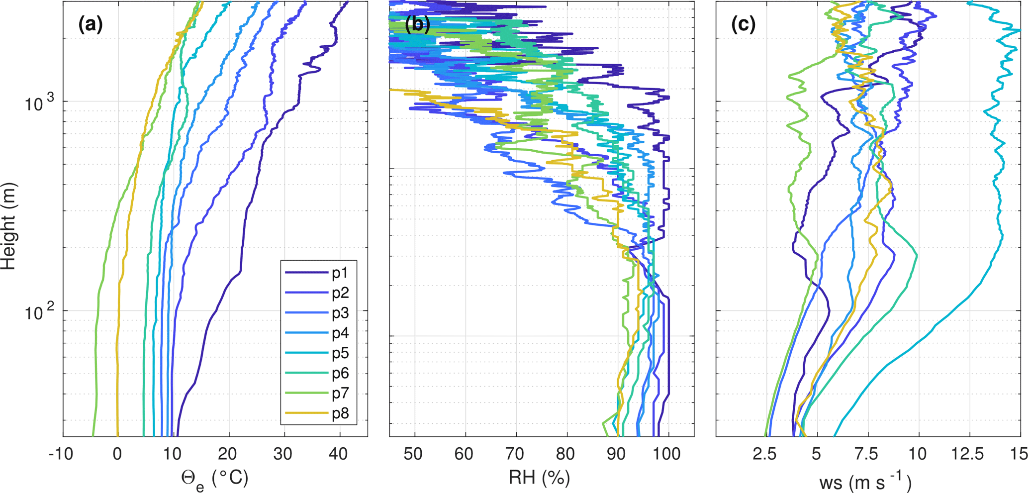
Figure 13Median profiles of (a) equivalent potential temperature, (b) RHw, and (c) wind speed for the eight key periods of the campaign.

Figure 14Statistics on surface mixed layer depth, main inversion base height, main inversion depth, and strength for the whole campaign and for the eight key periods.
5.2 Thermodynamic development
The vertical structure of the atmosphere during P1 (in the MIZ) shows distinct differences from the other periods within the central pack ice. In the MIZ, the air was coming from the south-east, advecting warm air over the melting sea ice towards the location of the ship, resulting in a stably stratified air mass (Fig. 13a). Equivalent potential temperature profiles are strongly stratified in the lowest 150 m, followed by a layer of weaker stratification up to around 650 m. The inversion statistics show that this period was dominated by strong and deep surface inversions (Fig. 14). Within the central pack ice, the thermodynamic structure of the atmosphere gradually changed from P2 to P3, with a reduction in stability (Fig. 13a) and a slight increase of the main inversion base height, but the inversions remained quite strong and deep (Fig. 14). P4 and P5 show quite distinct inversion characteristics. The median inversion base height is nearly 1000 m higher than in P3 (Fig. 14), but inversions were thinner and weaker. This is most likely caused by the strong synoptic activity during these periods with several frontal systems dominating the thermodynamic structure of the atmosphere. P5 was also the period with the highest wind speeds (Fig. 13c). P6 was partly influenced by a low-pressure system, also causing higher wind speeds (Fig. 13c) and most likely causing the wide spread of inversion base heights (Fig. 14). P7 was influenced by high pressure, resulting in more stable and very cold conditions (Fig. 13a). The main capping inversions were rather strong and low with a median base height of about 200 m. The final period has a low median main inversion base height of about 400 m but shows high variability as indicated by the 25th and 75th percentile (Fig. 14). It is also warmer than the previous period and has higher median wind speeds.
Table 3Percentage of coupled and decoupled boundary layer conditions for the whole campaign and for the eight key periods. Furthermore, the relative amount of the decoupling type is given – either by a weaker inversion below the main inversion or by the BL being stable, meaning decoupling by a surface inversion.
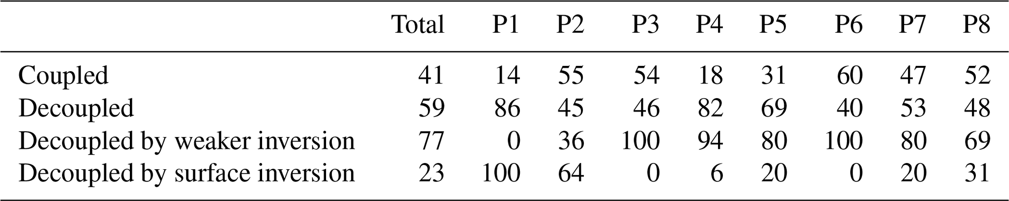
One important characteristic of the Arctic BL, particularly in the summer, is a frequent decoupling of the SML and the cloud mixed layer (CML) (Shupe et al., 2013; Brooks et al., 2017), a feature that models often fail to represent (Birch et al., 2012; Sotiropoulou et al., 2016). This is in particular relevant when investigating local aerosol production as a source of CCN or INPs and their impact on cloud. These particles can only affect cloud properties if they are mixed up to the clouds. Surface processes can be decoupled from the clouds via a secondary weak inversion below the main inversion or by a surface inversion, i.e. stable conditions. An overview of the relative amount of coupling and decoupling and the respective process of decoupling is listed in Table 3. P1 was mostly decoupled by surface inversions. P2 and P3 were decoupled for around 45 % of the time, where P2 still experienced a lot of surface inversions, whereas during P3 no surface inversions were observed. The median SML height was 155 and 170 m for P2 and P3, respectively, but the spread of SML heights was much wider for P2, reaching down to 0 m, representing the frequent occurrence of surface inversions (Fig. 14a). P4 and P5 were decoupled for 82 and 69 % of the time, respectively, with a much deeper SML than during the previous periods (Fig. 14a). Conditions during P6 were quite different, and the BL was decoupled only 40 % of the time with rather deep SMLs. The quite cold period P7 was decoupled 53 % of the time with particularly shallow SMLs. The median SML height was only 75 m. The last period was decoupled 48 % of the time, with one-third of the decoupling caused by a surface inversion.
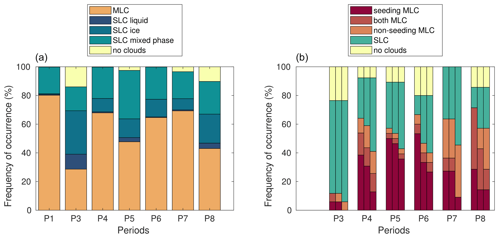
Figure 15(a) Frequency of occurrence of different types of single-layer clouds (SLCs), multi-layer clouds (MLCs), and no clouds from the Cloudnet results for all available key periods. P2 was excluded from the analysis as no radar data were available. (b) Frequency of occurrence of no clouds, SLCs, and potentially seeding and non-seeding MLCs using the method of Vassel et al. (2019) for assumed ice crystal sizes of 400 µm (left), 200 µm (middle), and 100 µm (right).
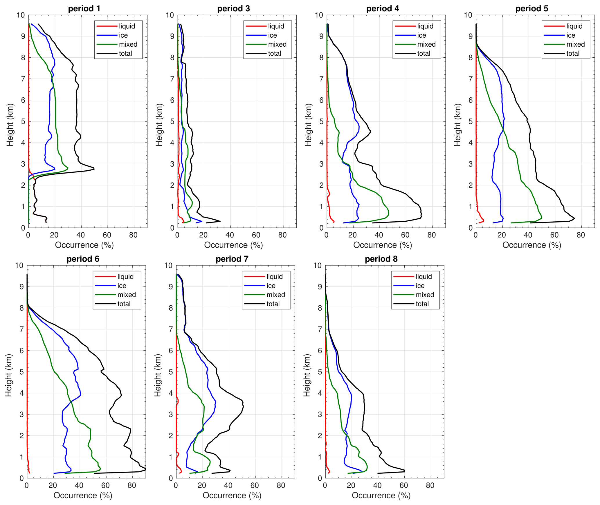
Figure 16Mean cloud occurrence per volume for different cloud types (colour coded), obtained from the Cloudnet target classification product for the eight key periods.
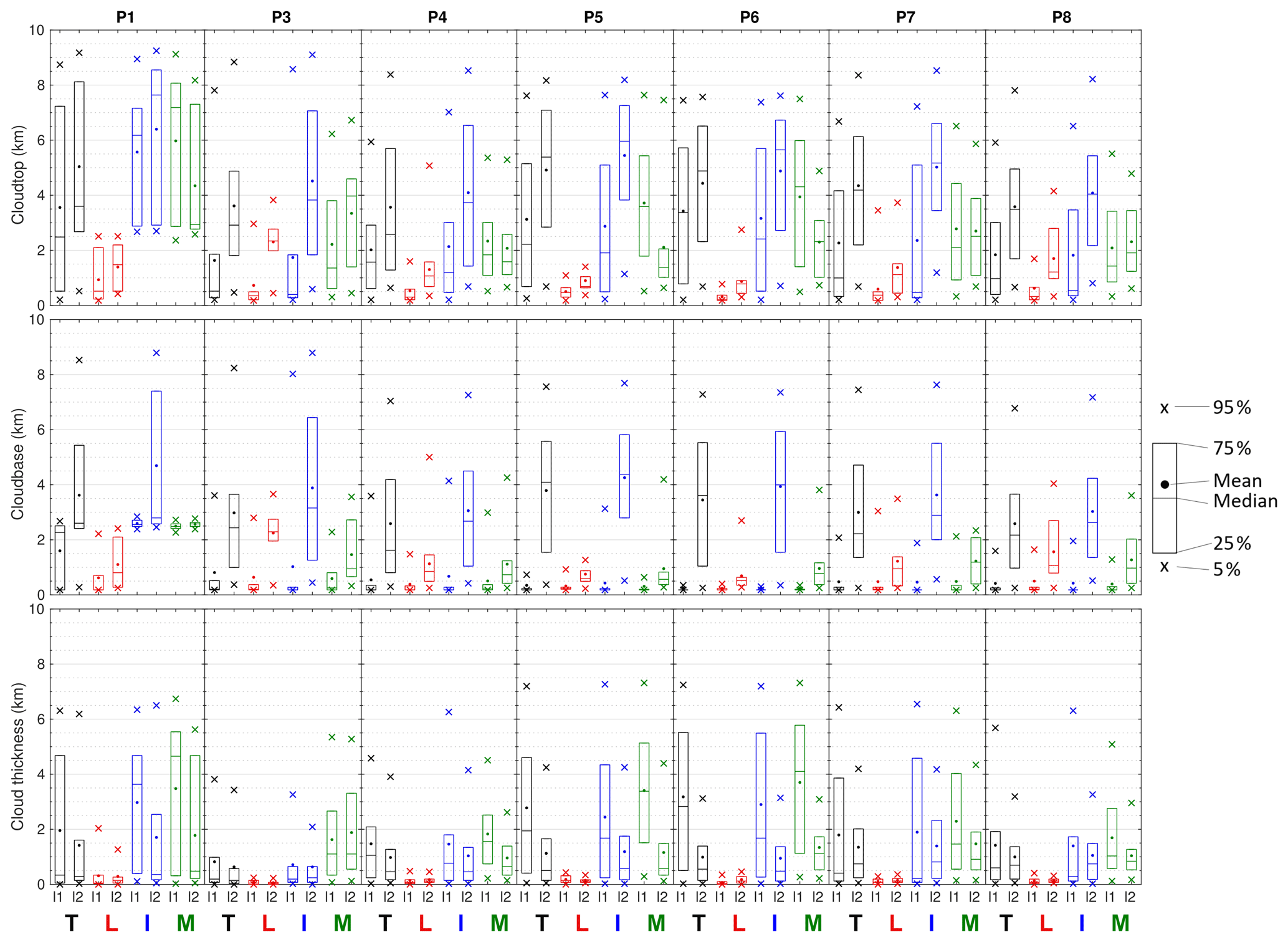
Figure 17Statistical overview of cloud top height (top row), cloud base height (middle row), and geometrical thickness (bottom row) for the eight key periods of AO2018. The colours indicate the different cloud types, total (T), liquid (L), ice (I), and mixed-phase (M) clouds. Results for the lowest two cloud layers (l1 and l2) are shown.
5.3 Cloud characteristics
Frequency of occurrence of single- and multi-layer clouds for each period is shown in Fig. 15a. Further analysis of potentially seeding and non-seeding multi-layer clouds is shown for P3–P7, for times within 60 min of a radiosonde profile (Fig. 15b). Cloud occurrence probability distributions are shown in Fig. 16, and statistics of cloud top, base, and thickness for the first two layers in Fig. 17. During P1 multiple cloud layers were present for 80 % of the time, and single-layer cloud occurrence was dominated by mixed-phase clouds. All clouds below 2.5 km were liquid clouds, while above this level mixed-phase and ice clouds reached up to 9.0 km (Fig. 15). The cloud layer statistics for P1 (Fig. 17) show these ice and mixed-phase clouds to be deep if they are the first cloud layer; they most likely consist of several cloud layers with precipitating ice in between. These were predominantly precipitating frontal clouds (Fig. 7d).
During P3 nearly 60 % of the Cloudnet profiles had a single cloud layer, and about 14 % showed no cloud layer (Fig. 15a). The method of Vassel et al. (2019) showed a slightly higher percentage of no clouds (24 %) and also single-layer clouds (65 %). The remaining multi-layer clouds all showed potential for seeding. Overall, there is a very low cloud fraction per volume for all heights, with a total maximum of 30 % in the lowest 500 m and below 20 % higher up (Fig. 16). First-layer clouds were mostly either shallow liquid and ice clouds or deeper mixed-phase clouds, which are most likely seeding multi-layer clouds as shown before (Fig. 17). For times with multiple cloud layers, the statistics for the second cloud layer show very thin liquid clouds at about 2.4 km height, thin ice clouds with a median cloud base height of 3.2 km, or low-level deep mixed-phase clouds. P3 is the only period showing a second layer of liquid clouds with such predominantly high cloud bases.
P4 was influenced by a low-pressure system moving anticlockwise around the measurement location (Fig. 4a). This resulted in multiple cloud layers for about 68 % of the time and much higher cloud occurrence than in P3, with a maximum cloud fraction of 70 % below 1000 m and a secondary maximum of 30 % at around 4500 m (Fig. 16). The potential of seeding for multi-layer mixed-phase or ice cloud cases is given 44 % of the time (Fig. 15b). The cloud statistics for P4 show that liquid clouds are very thin and occur predominantly below 1.1 km, with a median cloud thickness of 72 and 120 m and cloud tops of 300 and 1070 m for first- and second-layer clouds, respectively. First-layer mixed-phase clouds have a median cloud base at 215 m and a median cloud top at 1835 m, and second-layer clouds have a median cloud base at 730 m and cloud top at 1580 m. Mixed-phase and liquid clouds predominantly occur below 2 km, and clouds at higher altitudes are predominantly ice clouds. Ice cloud statistics show a large difference between first- and second-layer clouds. First-layer clouds have a median cloud base and top of 180 and 1190 m, respectively, whereas second-layer ice clouds have a large variability of cloud bases and tops, with median values of 2700 and 3730 m.
P5 and P6 show similar cloud characteristics. Cloud fraction per volume was over 70 % below 1 km for P5 and over 80 % for P6, which is the highest occurrence frequency of all eight periods (Fig. 16). Cloud fraction above 1 km was also high, more than 60 % up to 5 km. Mixed-phase clouds dominated up to 4.5 km in P5 and 3.5 km during P6. Statistics of cloud base, top, and thickness are comparable for P5 and P6. First-layer mixed-phase clouds had a median thickness of 4100 m. They were thicker than liquid and ice clouds and also thicker than during the other periods, except P1. First-layer ice clouds were also thicker than during the other periods, with median values of 1700 m. Second-layer ice clouds show higher median cloud bases compared to the other periods, at 4380 and 3995 m for P5 and P6, respectively. The seeding analysis shows that the potential for multi-layer seeding clouds is particularly high during P5 and P6 (Fig. 15b), meaning that the extremely thick mixed-phase and ice clouds detected in Cloudnet are most likely multiple cloud layers with ice crystals in between.
During P7 multiple cloud layers were present for nearly 70 % of the time. Approximately half of the time, seeding between cloud layers was detected. Cloud fraction peaks at around 3.5 km with a secondary maximum below 1.0 km (Fig. 15). Overall, first-layer clouds were thinner than in P4 to P6, but second-layer clouds, in particular ice clouds, were thicker than in previous periods, with a median value of 815 m.
For P8 statistics show that no clouds were detected for about 10 % of the time and about 47 % of the time single-layer clouds were present. The potential for seeding between cloud layers was high. The highest cloud fraction was observed in the lower levels, at 300 m with a secondary maximum of about 30 % at 4 km. Clouds, in particular first-layer mixed-phase clouds, were rather thin compared to the other periods with a median cloud thickness of 840 m, and second-layer ice clouds had a lower cloud base than during the rest of the freeze periods (P5 to P7).
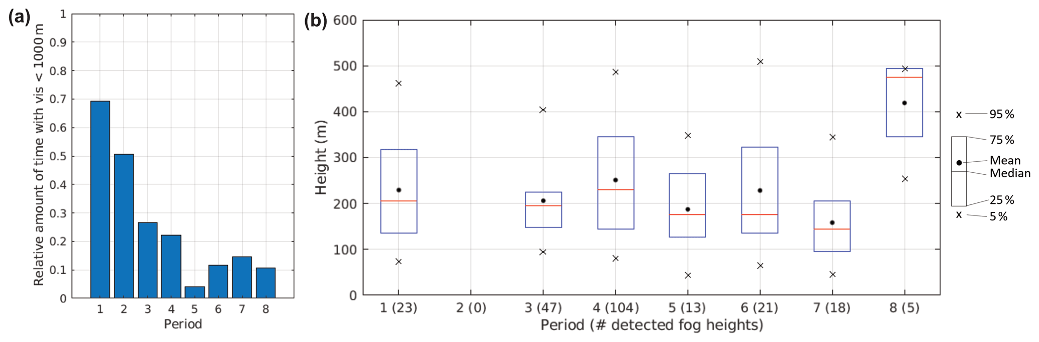
Figure 18Fog statistics. Relative amount of time with visibility <1000 m for each period and statistics of fog depths for each period where data were available (in period 2 no radar data were available).
Figure 18 shows the relative amount of fog occurrence during each period and the respective fog depths. P1 was the foggiest, with visibility below 1 km for 70 % of the time, followed by P2, with fog present around 50 % of the time. P3 and P4 had much fewer fog episodes, with 27 and 22 %, respectively. P5 was mostly fog free, and P6–P8 had fog around 12 to 15 % of the time. Fog depths are shown in Fig. 18b. These are quite similar throughout the measurement campaign, showing slightly higher median depths for P1–P4 than for P5–P7. P8 shows unusually deep fog layers with a calculated fog depth of over 400 m. However, radar RHI scans were only available for the first 3 d of P8, and only 10 % of the fog occurred within these 3 d. Hence, the calculated fog depth of over 400 m may not be representative of the total fog conditions during P8.
Here we compare the AO2018 observations with those from previous campaigns, providing insight into common features and significant differences. We compare the 2018 observations with the expeditions AOE1996, AOE2001, ASCOS, and AO2016, as these campaigns all operated in the central Arctic Ocean during the melt–freeze transition (Fig. 1, Table 1). Additional comparison is also made with results from SHEBA (Surface Heat Budget of the Arctic Ocean) in the Chukchi Sea during August and September 1998 and ACSE (Arctic Clouds in Summer Experiment) along the Siberian Shelf in 2014 where possible.
From a large-scale perspective the conditions during AO2018 are most similar to those of ASCOS, with low pressure over the Canadian Arctic Archipelago and over the Barents Sea (Tjernström et al., 2012). However, the strong high-pressure centre over the Canada Basin was absent in 2018. Instead of being in a clear anticyclonic circulation, as during ASCOS, or a clear cyclonic flow from one low-pressure centre – as during AOE2001, AOE1996, and SHEBA (Tjernström et al., 2012) – AO2018 sat between two low-pressure areas. As a result, several low-pressure systems propagated westward around the pole, influencing the AO2018 measurement campaign. A clear difference to ASCOS is the timing of the low-pressure systems. During ASCOS most of the storms happened in early and mid-August, at the beginning of the campaign and the installation of the ice camp, while the later ice drift period was in rather calm conditions. During AO2018 the low-pressure systems passed over the measurement site throughout the campaign, with most of the strong low-pressure systems influencing the ice drift measurements from mid-August into September.
This strong synoptic activity during AO2018 resulted in a vertical structure of the atmosphere that differed to the earlier campaigns. The vertical probability distribution of the equivalent potential temperature (Fig. 7a) shows two predominant BL depths: one near-neutrally stratified layer up to 400 to 500 m and another near-neutrally stratified layer up to ∼1.5 km. In contrast, the results from the previous campaigns were very consistent with only one dominating mixed-layer height of about 300–400 m (Tjernström et al., 2012). The AO2018 moisture profile is, however, consistent with earlier campaigns showing a layer with very high RH up to about 800 to 1000 m (e.g. Tjernström et al., 2012; Sedlar et al., 2011; Devasthale et al., 2011).

Figure 19Statistics on surface mixed layer depth, main inversion base height, strength, and depth for six campaigns: AO2018, AO2016, ACSE, ASCOS, AOE2001 and SHEBA.
To better compare the inversion characteristics, statistics were calculated using radiosonde profiles for all available campaigns (Fig. 19). The median heights of the main capping inversion bases for all campaigns are in the range of 310 to 570 m, with ASCOS having the highest median inversion base heights. AO2018 has a much wider distribution than the other campaigns, with the 25th and 75th percentile at 135 and 1500 m, respectively. The other campaigns' third quartile ranged from 860 to 1200 m. AO2018 inversions were shallower than during AOE2001, ASCOS, and ACSE but comparable to the other two, and the inversion strengths were comparable to AO2016, AOE2001, and SHEBA.
Another typical feature of Arctic BLs is the decoupling of the SML from the CML. This means that a transfer of heat, moisture, and aerosols between the surface and the clouds aloft is often inhibited. During AO2018 decoupling with a distinct SML was observed 45 % of the time, and surface inversions 14 % of the time. The rest of the time the BL was coupled. For comparison, Brooks et al. (2017) found the ASCOS boundary layer to be decoupled 48 % of the time during the ice drift and 76 % of the time during a period with a single deck of stratocumulus. Sotiropoulou et al. (2014) found similar results for a longer cloud-covered time period, with a decoupling frequency of 72 %. If all available radiosonde profiles for the ASCOS campaign are considered (i.e. including the transit into and out of the ice), the decoupling frequency is 57.2 %, similar to the frequency of decoupling observed during ACSE (56.9 %), AOE2001 (55.1 %), and SHEBA (57.3 %). AO2016 had less frequently decoupled boundary layer conditions: only 45.2 % of the time.
The near-surface conditions during AO2018 were similar to those observed during the other campaigns as analysed in Tjernström et al. (2012). Before the freeze-up, temperatures were around 0 ∘C with occasional brief cooler periods, mostly resulting from cloud-free conditions (Tjernström, 2005; Sedlar et al., 2011). RH, wind speeds, and visibility were also similar to the ranges observed in the other campaigns. The date of the start of freeze-up agrees well with other studies in the central Arctic, showing that the freeze-up occurs in the second half of August or early September (e.g. Rigor et al., 2000; Overland et al., 2008; Tjernström et al., 2012; Sedlar et al., 2011). The surface fluxes are also generally similar to those observed during the other campaigns, in particular ASCOS, but there are notable differences to the AOE1996, AOE2001, and SHEBA incoming solar radiation distributions. AO2018 had a pronounced peak at 50 W m−2 and only a few cases with higher solar radiation up to 250 W m−2, whereas AOE1996, AOE2001, and SHEBA peaked at higher values and had a wider distribution; this might be caused by the slightly different campaign durations and locations. AO2018 was longer than most of the summer campaigns and, hence, had more cases with low incoming radiation. Furthermore, SHEBA was located further south, and the smallest daily solar zenith angles therefore were smaller, resulting in a wider distribution with higher values.
As well as the difference in the thermodynamic vertical structure, cloud characteristics for AO2018 differed from former campaigns. The vertical cloud fraction distribution for AO2018 (Fig. 10) showed a maximum below 1 km, similar to ACSE and ASCOS (compare Fig. 9 in Achtert et al., 2020). The peak for AO2018 was, however, not as pronounced as during ASCOS. AO2018 had a near absence of liquid clouds and a much smaller number of mixed-phase clouds than during previous campaigns. Another difference during the freeze period was the much higher cloud fraction between 1 and 4 km. This was above 50 % during AO2018 but only ∼30 % during ASCOS and 10 % during ACSE (Achtert et al., 2020). This can most likely be attributed to the multiple low-pressure systems passing the AO2018 track during the second half of the campaign, bringing deep-reaching frontal cloud systems. Compared to ACSE and ASCOS, the much higher fraction of ice clouds between 1 and 4 km is noticeable, which could result from secondary ice formation due to seeding of the lower clouds from falling ice precipitation from higher clouds. The few liquid clouds were considerably thinner than during ACSE, with a median depth of 95 m during AO2018 compared to 220 m during ACSE (Achtert et al., 2020). This might be attributed to the location of the campaigns, with ACSE being farther south than AO2018, leading to overall warmer temperatures and more open water, and hence more favourable conditions for liquid clouds. Ice clouds were considerably thicker than during ACSE, with median values of 400 to 600 m compared to around 250 m during ACSE (Achtert et al., 2020).
Fog occurred 21 % of the time during AO2018, less than during ASCOS (25 %) but more often than during AOE2001 and AOE1996 (10 %–15 %, Tjernström et al., 2012). Fog depths were studied for the first time here and, hence, cannot be compared with the other campaigns.
This paper provides an overview of the atmospheric measurements and conditions during AO2018, which took place on the icebreaker Oden in the central Arctic Ocean from 1 August until 21 September 2018. The results are also compared with those of previous Arctic field campaigns from the summers of 1996, 1998, 2001, 2008, 2014, and 2016.
The large-scale atmospheric conditions had the campaign under the influence of two low-pressure areas. One was centred over the Canadian Arctic Archipelago to the west and the other over the Barents Sea to the east, with the AO2018 track located in the middle. This resulted in several synoptic storms passing over the AO2018 track, in particular from mid-August until the end of the campaign in late September. AO2018, like previous campaigns, featured a moist, near-neutrally stratified BL; however there were two distinct regimes in vertical structure. One featured a well-mixed BL up to about 300 to 400 m, while the other showed a well-mixed layer up to about 1500 m. This is also represented in the wide spread of the inversion base heights. Fifty per cent of the inversion bases were below 370 m; another 25 % were considerably higher, up to 1500 m; and the rest even higher. The humidity profiles showed only one regime, similar to previous studies with a 1 km deep moist boundary layer. The boundary layer was decoupled 59 % of the time.
In contrast to the vertical structure, near-surface conditions shared the same common features as previous campaigns. During the melt period the near-surface temperature was mostly between −2 and 0 ∘C. After the start of the freeze-up, around 28 August, temperatures decreased, reaching a minimum of about −15 ∘C. The near-surface atmosphere was very moist, with RH mostly above 90 %. Near-surface winds were mostly between 2 and 7 m s−1 but occasionally reached up to 16 m s−1 during the passage of low-pressure systems. Surface energy fluxes were similar to the range observed in previous campaigns. Net short-wave radiation peaked at 10 W m−2 with a positive tail. The peak corresponds to the mostly cloudy conditions, and the tail reflects the few cloud-free conditions. The net long-wave radiation probability distributions peak at −5 W m−2, having a long tail to smaller values. Turbulent fluxes were as expected very small, peaking at −10 to 0 W m−2 for sensible heat and −5 W m−2 for the latent heat flux.
The cloud occurrence was high throughout the campaign, dominated by low-level clouds but with a substantial amount of mid-level clouds. In particular during the freeze-up the cloud fraction was above 50 % between 1 and 4 km, much higher than for the earlier expeditions. The unexpected high occurrence of multiple cloud decks and the absence of prolonged periods with shallow, single-layer stratocumulus clouds are most likely attributable to the strong cyclonic activity throughout the whole campaign. Several weaker low-pressure systems influenced the AO2018 measurements in the first half of August, and multiple strong low-pressure systems associated with frontal cloud systems occurred in the second half of August until the end of the measurement campaign in September. This also resulted in a strongly reduced occurrence of liquid clouds. Most of the clouds observed were either ice or mixed-phase clouds. The lowest cloud layer was dominated by mixed-phase clouds, while during times with multiple cloud layers the second cloud layer was dominated by ice clouds. Cloud thickness depended strongly on the cloud type, with a median cloud thickness of the lowest two layers of only 95 m for liquid clouds and 530 m for ice clouds. For mixed-phase clouds, thickness also varied strongly between first- and second-layer clouds, with 1700 m for first-layer mixed-phase clouds and 740 m for second-layer clouds. However, what cannot be ruled out is that the Cloudnet statistics for mixed-phase and ice clouds might contain multiple cloud layers with falling ice in between the cloud layers, detected as one cloud; the Cloudnet algorithm cannot distinguish between falling ice and cloud ice particles. The method of Vassel et al. (2019) showed potential seeding for 48 % of the analysed data. Falling ice from higher clouds into lower cloud layers might also be responsible for the high amount of ice clouds at relatively low heights, as these ice particles might trigger secondary ice formation in the lower clouds. Visibility measurements indicated frequent occurrence of fog, but with very variable persistence; fogs became somewhat less frequent during the freeze-up. Analysis of radar RHI scans revealed that fog layer depths were predominantly less than 200 m.
Overall, the meteorological results from AO2018 summarised here provide a guide for further investigation. For instance, reanalysis data already show an increase of Arctic cyclone activity during the second half of the 20th century (Zhang et al., 2004), and global and regional climate models suggest a further increase of cyclone activity during summer over the Central Arctic by the end of the 21st century (Orsolini and Sorteberg, 2009; Nishii et al., 2015; Akperov et al., 2019). This study shows that strong cyclonic activity is associated with changes of the thermodynamic structure, the cloud types, and the vertical cloud distribution. So it raises the question of whether this was an exceptional year or if these changes are representative of climatological change in Arctic summer atmospheric conditions.
UK contributions, as well as selected other data, are available within the associated data collection in the Centre for Environmental Data Analysis (CEDA) archives (http://archive.ceda.ac.uk/, last access: 4 January 2021). Other cruise data are available from the Bolin Centre for Climate Research MOCCHA/AO2018 holdings (http://bolin.su.se/data, last access: 4 January 2021), including the ship navigation data (https://catalogue.ceda.ac.uk/uuid/9405b2f8056947609da4bcc0bc88c5e8, last access: 4 January 2021; Brooks and Vüllers, 2020), Cloudnet data (https://doi.org/10.17043/ao2018-cloudnet-3; Vüllers et al., 2020), radiosonde data (https://doi.org/10.17043/ao2018-radiosonde-2; Prytherch et al., 2019), present weather sensor data (https://doi.org/10.17043/ao2018-present-weather; Prytherch, 2019), weather station data (https://doi.org/10.17043/ao2018-misu-weather-2; Prytherch, 2020), and micrometeorological data (https://doi.org/10.17043/ao2018-micromet-oden-3; Prytherch and Tjernström, 2020).
JV analysed the data set and prepared the manuscript together with IMB, MT, JP, and PA. IMB, PA, MT, and JP performed the measurements during AO2018. AB conducted the ice seeding analysis for an undergraduate dissertation, supervised by PA. All authors contributed to the discussion of the results and revision of the manuscript.
The authors declare that they have no conflict of interest.
The Atmospheric Measurements and Observations Facility (AMOF) of the UK National Centre for Atmospheric Science (NCAS) provided the cloud radar, HALO lidar, RPG HATPRO radiometer, Campbell ceilometer, radiosounding station, and Micro Rain Radar. The soundings were supported by Environment and Climate Change Canada in collaboration with the Year of Polar Prediction, Polar Prediction Project. Additional flux observations on the ice were supported by the Bolin Centre for Climate Research. The Swedish Polar Research Secretariat (SPRS) provided access to the icebreaker (I/B) Oden and logistical support in collaboration with the US National Science Foundation. We would like to thank Capt. Mattias Petersen and the crew of Oden for their invaluable support throughout the field campaign. Thanks also to the Chief Scientists Caroline Leck and Patricia Matrai for the planning and coordination of AO2018. Thanks to Luisa Ickes for her support with setting up the seeding analysis.
This research has been supported by the UK Natural Environment Research Council (NERC) (grant no. NE/R009686/1) and the Knut and Alice Wallenberg Foundation (grant no. 2016-0024).
This paper was edited by Lynn M. Russell and reviewed by two anonymous referees.
Achtert, P., Brooks, I. M., Brooks, B. J., Moat, B. I., Prytherch, J., Persson, P. O. G., and Tjernström, M.: Measurement of wind profiles by motion-stabilised ship-borne Doppler lidar, Atmos. Meas. Tech., 8, 4993–5007, https://doi.org/10.5194/amt-8-4993-2015, 2015.
Achtert, P., O'Connor, E. J., Brooks, I. M., Sotiropoulou, G., Shupe, M. D., Pospichal, B., Brooks, B. J., and Tjernström, M.: Properties of Arctic liquid and mixed phase clouds from ship-borne Cloudnet observations during ACSE 2014, Atmos. Chem. Phys. Discuss., https://doi.org/10.5194/acp-2020-56, in review, 2020.
Akperov, M., Rinke, A., Mokhov, I. I., Semenov, V. A., Parfenova, M. R., Matthes, H., Adakudlu, M., Boberg, F., Christensen, J. H., Dembitskaya, M. A., Dethloff, K., Fettweis, X., Gutjahr, O., Heinemann, G., Koenigk, T., Koldunov, N. V., Laprise, R., Mottram, R., Nikiéma, O., Sein, D., Sobolowski, S., Winger, K., and Zhang, W.: Future projections of cyclone activity in the Arctic for the 21st century from regional climate models (Arctic-CORDEX), Glob. Planet. Change, 182, 103005, https://doi.org/10.1016/j.gloplacha.2019.103005, 2019.
Andreas, E. L., Guest, P. S., Persson, P. O. G., Fairall, C. W., Horst, T. W., Moritz, R. E., and Semmer, S. R.: Near-surface water vapor over polar sea ice is always near ice saturation, J. Geophys. Res.-C Ocean., 107, 8033, https://doi.org/10.1029/2000jc000411, 2002.
Birch, C. E., Brooks, I. M., Tjernström, M., Shupe, M. D., Mauritsen, T., Sedlar, J., Lock, A. P., Earnshaw, P., Persson, P. O. G., Milton, S. F., and Leck, C.: Modelling atmospheric structure, cloud and their response to CCN in the central Arctic: ASCOS case studies, Atmos. Chem. Phys., 12, 3419–3435, https://doi.org/10.5194/acp-12-3419-2012, 2012.
Boeke, R. C. and Taylor, P. C.: Evaluation of the Arctic surface radiation budget in CMIP5 models, J. Geophys. Res.-Atmos., 121, 8525–8548, https://doi.org/10.1002/2016JD025099, 2016.
Brooks, I. and Vüllers, J.: Microbiology-Ocean-Cloud Coupling in the High Arctic (MOCCHA): SPRS Icebreaker Oden ship navigation data. Centre for Environmental Data Analysis, available at: https://catalogue.ceda.ac.uk/uuid/9405b2f8056947609da4bcc0bc88c5e8 (last access: 4 January 2021), 2020.
Brooks, I. M., Tjernström, M., Persson, P. O. G., Shupe, M. D., Atkinson, R. A., Canut, G., Birch, C. E., Mauritsen, T., Sedlar, J., and Brooks, B. J.: The turbulent structure of the Arctic summer boundary layer during The Arctic Summer Cloud-Ocean Study, J. Geophys. Res., 122, 9685–9704, https://doi.org/10.1002/2017JD027234, 2017.
Brooks, M. E., Hogan, R. J., and Illingworth, A. J.: Parameterizing the Difference in Cloud Fraction Defined by Area and by Volume as Observed with Radar and Lidar, J. Atmos. Sci., 62, 2248–2260, https://doi.org/10.1175/JAS3467.1, 2005.
Colony, R., Appel, I., and Rigor, I.: Surface air temperature observations in the Arctic Basin. Tech. Memo. TM 1-92, Applied Physics Laboratory, University of Washington, Seattle, WA, 120 pp., 1992.
Devasthale, A., Sedlar, J., and Tjernström, M.: Characteristics of water-vapour inversions observed over the Arctic by Atmospheric Infrared Sounder (AIRS) and radiosondes, Atmos. Chem. Phys., 11, 9813–9823, https://doi.org/10.5194/acp-11-9813-2011, 2011.
Foken, T. and Wichura, B.: Tools for quality assessment of surface-based flux measurements, Agric. For. Meteorol., 78, 83–105, https://doi.org/10.1016/0168-1923(95)02248-1, 1996.
Graversen, R. G., Mauritsen, T., Tjernström, M., Källen, E., and Svensson, G.: Vertical structure of recent Arctic warming, Nature, 451, 53–57, https://doi.org/10.1038/nature06502, 2008.
Hartfield, G., Blunden, J., and Arndt, D. S.: A Look at 2017: Takeaway Points from the State of the Climate Supplement, B. Am. Meteorol. Soc., 99, 1527–1539, https://doi.org/10.1175/BAMS-D-18-0173.1, 2018.
Hodson, D. L. R., Keeley, S. P. E., West, A., Ridley, J., Hawkins, E., and Hewitt, H. T.: Identifying uncertainties in Arctic climate change projections, Clim. Dynam., 40, 2849–2865, https://doi.org/10.1007/s00382-012-1512-z, 2013.
Holland, M. M. and Bitz, C. M.: Polar amplification of climate change in coupled models, Clim. Dynam., 21, 221–232, https://doi.org/10.1007/s00382-003-0332-6, 2003.
Illingworth, A. J., Hogan, R. J., O'Connor, E. J., Bouniol, D., Brooks, M. E., Delanoé, J., Donovan, D. P., Eastment, J. D., Gaussiat, N., Goddard, J. W. F., Haeffelin, M., Baltink, H. K., Krasnov, O. A., Pelon, J., Piriou, J.-M., Protat, A., Russchenberg, H. W. J., Seifert, A., Tompkins, A. M., van Zadelhoff, G.-J., Vinit, F., Willén, U., Wilson, D. R. and Wrench, C. L.: Cloudnet, B. Am. Meteorol. Soc., 88, 883–898, https://doi.org/10.1175/BAMS-88-6-883, 2007.
Intrieri, J. M., Fairall, C. W., Shupe, M. D., Persson, P. O. G., Andreas, E. L., Guest, P. S., and Moritz, R. E.: An annual cycle of Arctic surface cloud forcing at SHEBA, J. Geophys. Res., 107, 8039, https://doi.org/10.1029/2000JC000439, 2002.
IPCC: Climate Change 2007: The Physical Science Basis. Contribution of Working Group I to the Fourth Assessment Report of the Intergovernmental Panel on Climate Change, Cambridge University Press, Cambridge, United Kingdom and New York, NY, USA, 2007.
IPCC: Climate Change 2013: The Physical Science Basis. Contribution of Working Group I to the Fifth Assessment Report of the Intergovernmental Panel on Climate Change, Cambridge University Press, Cambridge, United Kingdom and New York, NY, USA, 2013.
IPCC: Global warming of 1.5 ∘C. An IPCC Special Report on the impacts of global warming of 1.5 ∘C above pre-industrial levels and related global greenhouse gas emission pathways, in the context of strengthening the global response to the threat of climate change, edited by: Masson-Delmotte, V., Zhai, P., Pörtner, H.-O., Roberts, D., Skea, J., Shukla, P. R., Pirani, A., Moufouma-Okia, W., Péan, C., Pidcock, R., Connors, S., Matthews, J. B. R., Chen, Y., Zhou, X., Gomis, M. I., Lonnoy, E., Maycock, T., Tignor, M., and Waterfield, T., 2018.
Kalnay, E., Kanamitsu, M., Kistler, R., Collins, W., Deaven, D., Gandin, L., Iredell, M., Saha, S., White, G., Woollen, J., Zhu, Y., Chelliah, M., Ebisuzaki, W., Higgins, W., Janowiak, J., Mo, K. C., Ropelewski, C., Wang, J., Leetmaa, A., Reynolds, R., Jenne, R., Joseph, D., Kalnay, E., Kanamitsu, M., Kistler, R., Collins, W., Deaven, D., Gandin, L., Iredell, M., Saha, S., White, G., Woollen, J., Zhu, Y., Chelliah, M., Ebisuzaki, W., Higgins, W., Janowiak, J., Mo, K. C., Ropelewski, C., Wang, J., Leetmaa, A., Reynolds, R., Jenne, R., and Joseph, D.: The NCEP/NCAR 40-Year Reanalysis Project, B. Am. Meteorol. Soc., 77, 437–472, https://doi.org/10.1175/1520-0477(1996)077<0437:TNYRP>2.0.CO;2, 1996.
Leck, C., Nilsson, E. D., Bigg, E. K., and Bäcklin, L.: Atmospheric program on the Arctic Ocean Expedition 1996 (AOE-96): An overview of scientific goals, experimental approach, and instruments, J. Geophys. Res.-Atmos., 106, 32051–32067, https://doi.org/10.1029/2000JD900461, 2001.
Liu, Y., Key, J. R., Wang, X., Liu, Y., Key, J. R., and Wang, X.: The Influence of Changes in Cloud Cover on Recent Surface Temperature Trends in the Arctic, J. Climate, 21, 705–715, https://doi.org/10.1175/2007JCLI1681.1, 2008.
Mauritsen, T., Sedlar, J., Tjernström, M., Leck, C., Martin, M., Shupe, M., Sjogren, S., Sierau, B., Persson, P. O. G., Brooks, I. M., and Swietlicki, E.: An Arctic CCN-limited cloud-aerosol regime, Atmos. Chem. Phys., 11, 165–173, https://doi.org/10.5194/acp-11-165-2011, 2011.
Morrison, H., de Boer, G., Feingold, G., Harrington, J., Shupe, M. D., and Sulia, K.: Resilience of persistent Arctic mixed-phase clouds, Nat. Geosci., 5, 11–17, https://doi.org/10.1038/ngeo1332, 2012.
Nishii, K., Nakamura, H., and Orsolini, Y. J.: Arctic summer storm track in CMIP3/5 climate models, Clim. Dynam., 44, 1311–1327, https://doi.org/10.1007/s00382-014-2229-y, 2015.
Onarheim, I. H., Eldevik, T., Smedsrud, L. H., and Stroeve, J. C.: Seasonal and Regional Manifestation of Arctic Sea Ice Loss, J. Climate, 31, 4917–4932, https://doi.org/10.1175/JCLI-D-17-0427.1, 2018.
Orsolini, Y. J. and Sorteberg, A.: Projected Changes in Eurasian and Arctic Summer Cyclones under Global Warming in the Bergen Climate Model, Atmos. Ocean. Sc. Lett., 2, 62–67, https://doi.org/10.1080/16742834.2009.11446776, 2009.
Osborne, E., Richter-Menge, J., and Jeffries, M.: Arctic Report Card 2018, available at: https://www.arctic.noaa.gov/Report-Card (last access: 4 January 2021), 2018.
Overland, J. E., Wang, M., and Salo, S.: The recent Arctic warm period, Tellus A, 60, 589–597, https://doi.org/10.1111/j.1600-0870.2008.00327.x, 2008.
Pearson, G., Davies, F., and Collier, C.: An analysis of the performance of the UFAM pulsed Doppler lidar for observing the boundary layer, J. Atmos. Ocean. Tech., 26, 240–250, 2009.
Perovich, D. K., Richter-Menge, J. A., Jones, K. F., and Light, B.: Sunlight, water, and ice: Extreme Arctic sea ice melt during the summer of 2007, Geophys. Res. Lett., 35, L11501, https://doi.org/10.1029/2008GL034007, 2008.
Pithan, F. and Mauritsen, T.: Arctic amplification dominated by temperature feedbacks in contemporary climate models, Nat. Geosci., 7, 181–184, https://doi.org/10.1038/ngeo2071, 2014.
Prenni, A. J., Harrington, J. Y., Tjernstöm, M., DeMott, P. J., Avramov, A., Long, C. N., Kreidenweis, S. M., Olsson, P. Q., and Verlinde, J.: Can ice-nucleating aerosols affect arctic seasonal climate?, B. Am. Meteorol. Soc., 88, 541–550, https://doi.org/10.1175/BAMS-88-4-541, 2007.
Prytherch, J.: Present weather sensor visibility and precipitation data from the Arctic Ocean 2018 expedition, Dataset version 1.0, Bolin Centre for Climate Research, Stockholm University, https://doi.org/10.17043/ao2018-present-weather, 2019.
Prytherch, J.: Weather data from MISU weather station during the Arctic Ocean 2018 expedition, Dataset version 2.0, Bolin Centre Database, https://doi.org/10.17043/ao2018-misu-weather-2, 2020.
Prytherch, J. and Tjernström, M.: Micrometeorological data from icebreaker Oden's foremast during the Arctic Ocean 2018 expedition, Dataset version 3.0, Bolin Centre Database, https://doi.org/10.17043/ao2018-micromet-oden-3, 2020.
Prytherch, J., Yelland, M. J., Brooks, I. M., Tupman, D. J., Pascal, R. W., Moat, B. I., and Norris, S. J.: Motion-correlated flow distortion and wave-induced biases in air–sea flux measurements from ships, Atmos. Chem. Phys., 15, 10619–10629, https://doi.org/10.5194/acp-15-10619-2015, 2015.
Prytherch, J., Brooks, I. M., Crill, P. M., Thornton, B. F., Salisbury, D. J., Tjernström, M., Anderson, L. G., Geibel, M. C., and Humborg, C.: Direct determination of the air-sea CO2 gas transfer velocity in Arctic sea ice regions, Geophys. Res. Lett., 44, 3770–3778, https://doi.org/10.1002/2017GL073593, 2017.
Prytherch, J., Tjernström, M., Vuellers, J., Achtert, P., Brooks, I., Porter, G., and Adams, M.: Radiosonde data from the Arctic Ocean 2018 expedition, Dataset version 2.0, Bolin Centre Database, https://doi.org/10.17043/ao2018-radiosonde-2, 2019.
Richter-Menge, J., Jeffries, M. O., and Osborne, E.: The Arctic in “State of the Climate in 2017”, B. Am. Meteorol. Soc., 99, 143–173, https://doi.org/10.1175/2018BAMSStateoftheClimate.1, 2018.
Richter-Menge, J., Druckenmiller, M. L., and Jeffries, M. (Eds.): Arctic Report Card 2019, available at: https://www.arctic.noaa.gov/Report-Card (last access: 4 January 2021), 2019.
Rigor, I. G., Colony, R. L., Martin, S., Rigor, I. G., Colony, R. L., and Martin, S.: Variations in Surface Air Temperature Observations in the Arctic, 1979–97, J. Climate, 13, 896–914, https://doi.org/10.1175/1520-0442(2000)013<0896:VISATO>2.0.CO;2, 2000.
Sedlar, J., Tjernström M., Mauritsen, T., Shupe, M. D., Brooks, I. M., Persson, P. O. G., Birch, C. E., Leck, C., Sirevaag, A., and Nicolaus, M.: A transitioning Arctic surface energy budget: the impacts of solar zenith angle, surface albedo and cloud radiative forcing, Clim. Dynam., 37, 1643–1660, https://doi.org/10.1007/s00382-010-0937-5, 2011.
Serreze, M. C. and Barry, R. G.: Processes and impacts of Arctic amplification: A research synthesis, Glob. Planet. Change, 77, 85–96, https://doi.org/10.1016/j.gloplacha.2011.03.004, 2011.
Shupe, M. D.: Clouds at Arctic Atmospheric Observatories. Part II: Thermodynamic Phase Characteristics, J. Appl. Meteorol. Climatol., 50, 645–661, https://doi.org/10.1175/2010JAMC2468.1, 2011.
Shupe, M. D. and Intrieri, J. M.: Cloud Radiative Forcing of the Arctic Surface: The Influence of Cloud Properties, Surface Albedo, and Solar Zenith Angle, J. Climate, 17, 616–628, https://doi.org/10.1175/1520-0442(2004)017<0616:CRFOTA>2.0.CO;2, 2004.
Shupe, M. D., Walden, V. P., Eloranta, E., Uttal, T., Campbell, J. R., Starkweather, S. M., and Shiobara, M.: Clouds at Arctic Atmospheric Observatories. Part I: Occurrence and Macrophysical Properties, J. Appl. Meteorol. Climatol., 50, 626–644, https://doi.org/10.1175/2010JAMC2467.1, 2011.
Shupe, M. D., Persson, P. O. G., Brooks, I. M., Tjernström, M., Sedlar, J., Mauritsen, T., Sjogren, S., and Leck, C.: Cloud and boundary layer interactions over the Arctic sea ice in late summer, Atmos. Chem. Phys., 13, 9379–9399, https://doi.org/10.5194/acp-13-9379-2013, 2013.
Sotiropoulou, G., Sedlar, J., Tjernström, M., Shupe, M. D., Brooks, I. M., and Persson, P. O. G.: The thermodynamic structure of summer Arctic stratocumulus and the dynamic coupling to the surface, Atmos. Chem. Phys., 14, 12573–12592, https://doi.org/10.5194/acp-14-12573-2014, 2014.
Sotiropoulou, G., Sedlar, J., Forbes, R., and Tjernström, M.: Summer Arctic clouds in the ECMWF forecast model: An evaluation of cloud parameterization schemes, Q. J. Roy. Meteor. Soc., 142, 387–400, https://doi.org/10.1002/qj.2658, 2016.
Spreen, G., Kaleschke, L., and Heygster, G.: Sea ice remote sensing using AMSR-E 89 GHz channels, J. Geophys. Res., 113, C02S03, https://doi.org/10.1029/2005JC003384, 2008.
Stroeve, J. C., Kattsov, V., Barrett, A., Serreze, M., Pavlova, T., Holland, M., and Meier, W. N.: Trends in Arctic sea ice extent from CMIP5, CMIP3 and observations, Geophys. Res. Lett., 39, L16502, https://doi.org/10.1029/2012GL052676, 2012.
Taylor, P. C., Cai, M., Hu, A., Meehl, J., Washington, W., and Zhang, G. J.: A Decomposition of Feedback Contributions to Polar Warming Amplification, J. Climate, 26, 7023–7043, https://doi.org/10.1175/JCLI-D-12-00696.1, 2013.
Tjernström, M.: The summer Arctic boundary layer during the Arctic Ocean Experiment 2001 (AOE-2001), Bound.-Lay. Meteorol., 117, 5–36, https://doi.org/10.1007/s10546-004-5641-8, 2005.
Tjernström, M. and Graversen, R. G.: The vertical structure of the lower Arctic troposphere analysed from observations and the ERA-40 reanalysis, Q. J. Roy. Meteor. Soc., 135, 431–443, https://doi.org/10.1002/qj.380, 2009.
Tjernström, M., Leck, C., Persson, P. O. G., Jensen, M. L., Oncley, S. P., and Targino, A.: The summertime Arctic atmosphere: Meteorological measurements during the Arctic Ocean Experiment (AOE-2001), B. Am. Meteorol. Soc., 85, 1305–1321, https://doi.org/10.1175/BAMS-85-9-1305, 2004a.
Tjernström, M., Leck, C., Persson, P. O. G., Jensen, M. L., Oncley, S. P., and Targino, A.: Experimental equipment: An electronic supplement to “The summertime Arctic atmosphere: Meteorological measurements during the Arctic Ocean Experiment (AOE-2001)”, B. Am. Meteorol. Soc., 85, 1322–1322, https://doi.org/10.1175/BAMS-85-9-Tjernstrom, 2004b.
Tjernström, M., Birch, C. E., Brooks, I. M., Shupe, M. D., Persson, P. O. G., Sedlar, J., Mauritsen, T., Leck, C., Paatero, J., Szczodrak, M., and Wheeler, C. R.: Meteorological conditions in the central Arctic summer during the Arctic Summer Cloud Ocean Study (ASCOS), Atmos. Chem. Phys., 12, 6863–6889, https://doi.org/10.5194/acp-12-6863-2012, 2012.
Tjernström, M., Leck, C., Birch, C. E., Bottenheim, J. W., Brooks, B. J., Brooks, I. M., Bäcklin, L., Chang, R. Y.-W., de Leeuw, G., Di Liberto, L., de la Rosa, S., Granath, E., Graus, M., Hansel, A., Heintzenberg, J., Held, A., Hind, A., Johnston, P., Knulst, J., Martin, M., Matrai, P. A., Mauritsen, T., Müller, M., Norris, S. J., Orellana, M. V., Orsini, D. A., Paatero, J., Persson, P. O. G., Gao, Q., Rauschenberg, C., Ristovski, Z., Sedlar, J., Shupe, M. D., Sierau, B., Sirevaag, A., Sjogren, S., Stetzer, O., Swietlicki, E., Szczodrak, M., Vaattovaara, P., Wahlberg, N., Westberg, M., and Wheeler, C. R.: The Arctic Summer Cloud Ocean Study (ASCOS): overview and experimental design, Atmos. Chem. Phys., 14, 2823–2869, https://doi.org/10.5194/acp-14-2823-2014, 2014.
Vassel, M., Ickes, L., Maturilli, M., and Hoose, C.: Classification of Arctic multilayer clouds using radiosonde and radar data in Svalbard, Atmos. Chem. Phys., 19, 5111–5126, https://doi.org/10.5194/acp-19-5111-2019, 2019.
Vickers, D. and Mahrt, L.: Quality Control and Flux Sampling Problems for Tower and Aircraft Data, J. Atmos. Ocean. Tech., 14, 512–526, https://doi.org/10.1175/1520-0426(1997)014<0512:qcafsp>2.0.co;2, 1997.
Vihma, T., Pirazzini, R., Fer, I., Renfrew, I. A., Sedlar, J., Tjernström, M., Lüpkes, C., Nygård, T., Notz, D., Weiss, J., Marsan, D., Cheng, B., Birnbaum, G., Gerland, S., Chechin, D., and Gascard, J. C.: Advances in understanding and parameterization of small-scale physical processes in the marine Arctic climate system: a review, Atmos. Chem. Phys., 14, 9403–9450, https://doi.org/10.5194/acp-14-9403-2014, 2014.
Vüllers, J., Achtert, P., Brooks, I., Neely III, R., and Brooks, B.: Cloudnet remote sensing retrievals of cloud properties during the Arctic Ocean 2018 expedition, Dataset version 3.0, Bolin Centre Database, https://doi.org/10.17043/ao2018-cloudnet-3, 2020.
Wendisch, M., Macke, A., Ehrlich, A., Lüpkes, C., Mech, M., Chechin, D., Dethloff, K., Velasco, C. B., Bozem, H., Brückner, M., Clemen, H.-C., Crewell, S., Donth, T., Dupuy, R., Ebell, K., Egerer, U., Engelmann, R., Engler, C., Eppers, O., Gehrmann, M., Gong, X., Gottschalk, M., Gourbeyre, C., Griesche, H., Hartmann, J., Hartmann, M., Heinold, B., Herber, A., Herrmann, H., Heygster, G., Hoor, P., Jafariserajehlou, S., Jäkel, E., Järvinen, E., Jourdan, O., Kästner, U., Kecorius, S., Knudsen, E. M., Köllner, F., Kretzschmar, J., Lelli, L., Leroy, D., Maturilli, M., Mei, L., Mertes, S., Mioche, G., Neuber, R., Nicolaus, M., Nomokonova, T., Notholt, J., Palm, M., van Pinxteren, M., Quaas, J., Richter, P., Ruiz-Donoso, E., Schäfer, M., Schmieder, K., Schnaiter, M., Schneider, J., Schwarzenböck, A., Seifert, P., Shupe, M. D., Siebert, H., Spreen, G., Stapf, J., Stratmann, F., Vogl, T., Welti, A., Wex, H., Wiedensohler, A., Zanatta, M., and Zeppenfeld, S.: The Arctic Cloud Puzzle: Using ACLOUD/PASCAL Multiplatform Observations to Unravel the Role of Clouds and Aerosol Particles in Arctic Amplification, B. Am. Meteorol. Soc., 100, 841–871, https://doi.org/10.1175/BAMS-D-18-0072.1, 2019.
Zhang, X., Walsh, J. E., Zhang, J., Bhatt, U. S., Ikeda, M., Zhang, X., Walsh, J. E., Zhang, J., Bhatt, U. S., and Ikeda, M.: Climatology and Interannual Variability of Arctic Cyclone Activity: 1948–2002, J. Climate, 17, 2300–2317,, https://doi.org/10.1175/1520-0442(2004)017<2300:CAIVOA>2.0.CO;2, 2004.
https://www.misu.su.se/research/moccha-arctic-expedition-1.379414 (last access: 4 January 2021)
https://www.misu.su.se/research/2.55356/acas-project-1.408985 (last access: 4 January 2021)