Observational evidence of energetic particle precipitation NO_x (EPP-NO_x) interaction with chlorine curbing Antarctic ozone loss

We investigate the impact of the so-called energetic particle precipitation (EPP) indirect effect on lower stratospheric ozone, ClO, and ClONO₂ in the Antarctic springtime. We use observations from the Microwave Limb Sounder (MLS) and Ozone Monitoring Instrument (OMI) on Aura, the Atmospheric Chemistry Experiment – Fourier Transform Spectrometer (ACE-FTS) on SCISAT, and the Michelson Interferometer for Passive Atmospheric Sounding (MIPAS) on Envisat, covering the period from 2005 to 2017. Using the geomagnetic activity index Ap as a proxy for EPP, we find consistent ozone increases with elevated EPP during years with an easterly phase of the quasi-biennial oscillation (QBO) in both OMI and MLS observations. While these increases are the opposite of what has previously been reported at higher altitudes, the pattern in the MLS O₃ follows the typical descent patterns of EPP-NO_x. The ozone enhancements are also present in the OMI total O₃ column observations. Analogous to the descent patterns found in O₃, we also found consistent decreases in springtime MLS ClO following winters with elevated EPP. To verify if this is due to a previously proposed mechanism involving the conversion of ClO to the reservoir species ClONO₂ in reaction with NO₂, we used ClONO₂ observations from ACE-FTS and MIPAS. As ClO and NO₂ are both catalysts in ozone destruction, the conversion to ClONO₂ would result in an ozone increase. We find a positive correlation between EPP and ClONO₂ in the upper stratosphere in the early spring and in the lower stratosphere in late spring, providing the first observational evidence supporting the previously proposed mechanism relating to EPP-NO_x modulating Cl_x-driven ozone loss. Our findings suggest that EPP has played an important role in modulating ozone depletion in the last 15 years. As chlorine loading in the polar stratosphere continues to decrease in the future, this buffering mechanism will become less effective, and catalytic ozone destruction by EPP-NO_x will likely become a major contributor to Antarctic ozone loss.

1 Introduction

Our understanding of the causes of the Antarctic stratospheric ozone hole (Farman et al., 1985) relies on half a century of discoveries about the Earth's atmosphere: the Brewer–Dobson circulation (Brewer, 1949), which allows gases such as chlorofluorocarbons (CFCs) emitted in the tropical troposphere to be drawn into the southern polar atmosphere; the strong polar vortex in the Southern Hemisphere, which allows the polar stratosphere to become very cold, with a net downwelling effect pulling gases from the mesosphere and upper stratosphere into the lower stratosphere (Schoeberl and Hartmann, 1991); and polar stratospheric clouds (PSCs), forming in the very cold lower stratosphere which, with the reintroduction of sunlight in the early spring, enable the breakdown of chlorine reservoirs into simpler Cl_x ($=\mathrm{Cl}+\mathrm{ClO}$) molecules on the cloud surfaces (Solomon et al., 1986). Cl_x is effective at catalytically destroying ozone via one such chain of reactions:

$$\begin{array}{}\text{(R1)}& {\displaystyle }\mathrm{ClO}+\mathrm{O}\to \mathrm{Cl}+{\mathrm{O}}_{\mathrm{2}}\text{(R2)}& {\displaystyle }\mathrm{Cl}+{\mathrm{O}}_{\mathrm{3}}\to \mathrm{ClO}+{\mathrm{O}}_{\mathrm{2}}\end{array}$$

$$\text{Net}:\mathrm{O}+{\mathrm{O}}_{\mathrm{3}}\to \mathrm{2}{\mathrm{O}}_{\mathrm{2}}.$$

Other, more complicated reactions, such as with the ClO dimer, and heterogeneous reactions also destroy ozone (Brasseur and Solomon, 2005), but they will not be elaborated on further here.

In the lower stratosphere, Cl_x is, for most of the year, stored in reservoir species such as HCl and ClONO₂. Cl_x is activated from these species in heterogeneous reactions in the springtime – hence the importance of PSCs providing solid and liquid particles. As PSCs disappear with warming of the stratosphere as spring progresses, Cl_x is converted back to these reservoirs via reactions such as

$$\begin{array}{}\text{(R3)}& {\displaystyle }\mathrm{ClO}+\mathrm{OH}\to \mathrm{HCl}+{\mathrm{O}}_{\mathrm{2}}\text{(R4)}& {\displaystyle }\mathrm{Cl}+{\mathrm{HO}}_{\mathrm{2}}\to \mathrm{HCl}+{\mathrm{O}}_{\mathrm{2}}\text{(R5)}& {\displaystyle }\mathrm{ClO}+{\mathrm{NO}}_{\mathrm{2}}\stackrel{\mathrm{M}}{⟶}{\mathrm{ClONO}}_{\mathrm{2}}.\end{array}$$

Reactions (R3)–(R5) require the presence of HO_x ($=\mathrm{OH}+{\mathrm{HO}}_{\mathrm{2}}$) or NO_x ($=\mathrm{NO}+{\mathrm{NO}}_{\mathrm{2}}$) gases. This indicates that the presence of HO_x and NO_x gases in the lower and middle stratosphere plays a critical role as a limiter in Cl_x-driven O₃ loss until the eventual removal of Cl_x from the atmosphere via gravitational sedimentation of HCl.

In the context of polar ozone loss, in the past 20 years we have learned more about the impact of energetic particle precipitation (EPP). EPP is the flux of charged particles of solar and magnetospheric origin into the Earth's atmosphere. For the most part, this is made up of energetic electrons, with solar proton events (SPEs; the precipitation of energetic protons) being more sporadic (Seppälä et al., 2014). Energetic particles ionize the neutral atmosphere, and the resulting chain of reactions is a key source of NO_x and HO_x in the mesosphere and upper stratosphere. NO_x and HO_x act as catalysts in ozone-depleting reaction cycles such as

$$\begin{array}{}\text{(R6)}& {\displaystyle }{\mathrm{NO}}_{\mathrm{2}}+\mathrm{O}\to \mathrm{NO}+{\mathrm{O}}_{\mathrm{2}}\text{(R7)}& {\displaystyle }\mathrm{NO}+{\mathrm{O}}_{\mathrm{3}}\to {\mathrm{NO}}_{\mathrm{2}}+{\mathrm{O}}_{\mathrm{2}}\end{array}$$

$$\mathrm{Net}:\mathrm{O}+{\mathrm{O}}_{\mathrm{3}}\to \mathrm{2}{\mathrm{O}}_{\mathrm{2}}$$

and

$$\begin{array}{}\text{(R8)}& {\displaystyle }{\mathrm{HO}}_{\mathrm{2}}+\mathrm{O}\to \mathrm{HO}+{\mathrm{O}}_{\mathrm{2}}\text{(R9)}& {\displaystyle }\mathrm{HO}+{\mathrm{O}}_{\mathrm{3}}\to {\mathrm{HO}}_{\mathrm{2}}+{\mathrm{O}}_{\mathrm{2}}\end{array}$$

$$\text{Net}:\mathrm{O}+{\mathrm{O}}_{\mathrm{3}}\to \mathrm{2}{\mathrm{O}}_{\mathrm{2}},$$

and this EPP-driven ozone loss has been the topic of a large number of studies in the past decades. Note here that this role of HO_x and NO_x in ozone balance is the opposite to their ozone-loss-limiting impact via the build-up of reservoirs such as ClONO₂ in the lower and middle stratosphere.

The role of HO_x and NO_x in in situ EPP-driven ozone loss is now well known (see e.g. Jackman et al., 2008; Andersson et al., 2014). Polar ozone is also affected via the so-called “EPP indirect effect” (Randall et al., 2006). This refers to the process of transport of NO_x, produced by energetic particles at altitudes above 50 km (“EPP-NO_x”), to stratospheric altitudes, where it can contribute to ozone loss. When EPP occurs over the winter poles, the lack of sunlight results in an increased photochemical lifetime of NO_x, and the stable atmosphere provides a route for downwelling to stratospheric altitudes. This mechanism for EPP-NO_x descent is well-documented (see e.g. Siskind et al., 2000; Randall et al., 2005; Seppälä et al., 2007; Randall et al., 2007; Funke et al., 2014a, b; Gordon et al., 2020), and the depleting effect on ozone has been reported by a number of studies; for example, Randall et al. (2005) used observations from HALOE (HALogen Occultation Experiment), SAGE (Stratospheric Aerosol and Gas Experiment) II and III, POAM (Polar Ozone and Aerosol Measurement) II and III, MIPAS (Michelson Interferometer for Passive Atmospheric Sounding), and OSIRIS (Optical Spectrograph and InfraRed Imager System) to detect the NO_x increases in the Northern Hemisphere in January to March 2004 and reported ozone loss in March 2004 in the polar stratosphere. This was attributed to the combination of geomagnetic activity occurring in the winter and the reformation of the polar vortex following a sudden stratospheric warming (SSW) earlier in the winter. Seppälä et al. (2007) used the geomagnetic index Ap as a proxy for EPP levels. They correlated the 4-month wintertime average Ap value with the wintertime NO₂ data from GOMOS (Global Ozone Monitoring by Occultation of Stars) from 2002 to 2006 for both hemispheres, finding a robust linear relationship between the two. They also noted ozone loss and suggested that it is due to the descent of EPP-NO_x. Damiani et al. (2016) looked directly at ozone observations from the Solar Backscatter Ultraviolet Radiometer (SBUV) and the Microwave Limb Sounder (MLS, on the Aura satellite), together spanning the period from 1979 to 2014. They found ozone depletion of around 10 %–15% descending to 30 km (middle stratosphere) in September before disappearing. By comparing this with simultaneous HNO₃ enhancements in the Aura period (2004–2014), they were able to attribute the ozone depletion to NO_x increases from EPP (HNO₃ is a reservoir of NO_x).

Recent studies have looked at the descent of NO_x in the Southern Hemisphere in more detail. Funke et al. (2014a) used tracer correlations to extract EPP-NO_y (NO_y refers to all reactive nitrogen) from total NO_y and found that it reached altitudes as low as 20–25 km in the Southern Hemisphere by September. In the Antarctic spring, these correspond to altitudes where the ozone hole forms. Gordon et al. (2020) use a similar Ap scheme to Siskind et al. (2000) and Seppälä et al. (2007) to detect EPP-NO₂ in the stratospheric total NO₂ column using observations from the Ozone Monitoring Instrument (OMI). They found that the NO₂ column is significantly correlated with Ap until November. This presence in the NO₂ stratospheric column suggests that perturbations in EPP-NO₂ contribute significantly to the overall amount of NO₂ present in the stratosphere, as well as indicating that the EPP-NO_y reported by Funke et al. (2014a) remains in the atmosphere longer, until the breakdown of the polar vortex. Gordon et al. (2020) also found that accounting for the phase of the quasi-biennial oscillation (QBO) results in an increased correlation between Ap and the stratospheric NO₂ column in years with an easterly phase of the QBO, whereas the inverse was found for the westerly QBO phase. They postulate that this modulation by the QBO could reflect the influence of the QBO on the primary (non-EPP) NO_x source via transport from the equatorial region (see Strahan et al., 2015), combined with the effect that the QBO has on polar temperatures, which would influence the efficiency of removal of nitrogen species from the polar stratosphere. They show evidence that the QBO affects the temperature of the polar vortex in winter, with a warmer vortex in easterly QBO (eQBO) years. This leads to inhibited PSC formation and, hence, less effective removal of nitrogen species from the lower stratosphere.

This work

Here, we investigate the effect of EPP-NO_x on stratospheric ozone, focusing on the time of the ozone hole formation in the spring. Our analysis follows on from the results reported by Gordon et al. (2020), now focusing on the implications of the enhanced stratospheric NO₂ column on the Antarctic stratospheric ozone balance. We use ozone and chlorine species observations from three different satellite platforms (and four instruments), spanning the time period from 2005 to 2017, to get a more cohesive view on interactions taking place with EPP-NO_x, atmospheric chlorine, and ozone. We control our analysis for EPP levels (as proxied by the Ap index) and the phase of the QBO. Following from the initial analysis of ozone, we examine how EPP affects Cl_x activation in the springtime, by using ClO observations from MLS, and ClONO₂ from Atmospheric Chemistry Experiment – Fourier Transform Spectrometer (ACE-FTS) and MIPAS observations. We find that ozone tends to increase in years with high EPP and easterly QBO and suggest that this could be attributed to the combined effect of EPP and the QBO on the activation and deactivation of Cl_x.

2 Observations and methodology

2.1 MLS

We use ozone and ClO profiles (v4.2) from the Microwave Limb Sounder (MLS), on the Aura satellite (Schwartz et al., 2015; Santee et al., 2015). The data have been sorted according to Livesey et al. (2017), i.e removing data that do not meet the recommended quality standards. The O₃ profiles have been validated by Froidevaux et al. (2008), with further comparison to ground-based and other satellite measurements by Hubert et al. (2016). Here, we use stratospheric O₃ observations (15 to 50 km) with a vertical resolution of around 3 km and an uncertainty of no more than 4 %.

MLS ClO is valid throughout the stratosphere, although the lowermost altitudes (15–18 km) suffer from a negative bias. The bias, which has been uniform throughout the MLS period, is least significant in the polar region and is also systematic: each latitude is affected in the same way. We mitigate the effect of the bias by looking at anomalies, as any systematic bias will not affect the overall trend. As anomalies are differences from a mean, any shift is cancelled in subtraction. The vertical resolution of stratospheric ClO is around 3 km, and the error on individual profiles is around ±0.1 ppbv (Livesey et al., 2017). We do not use ClO from dusk until dawn (i.e. night-time) due to rapid conversion of ClO to the Cl₂O₂ dimer at night-time (Brasseur and Solomon, 2005). Excluding these measurements avoids the change in partitioning between day and night. We sort for day by only using profiles with a solar zenith angle $<\mathrm{90}{}^{\circ }$. MLS ClO profiles have been validated by Santee et al. (2008).

2.2 OMI

We analyse ozone total column data from the Dutch–Finnish-built Ozone Monitoring Instrument (OMI), also on Aura (Bhartia, 2012). Here, we use the OMI O₃ version 3, level 2 daily gridded product ($\mathrm{0.25}{}^{\circ }\times \mathrm{0.25}{}^{\circ }$ OMTO3G version 3). The algorithm is described by Bhartia (2002, 2007) with validation of OMI O₃ reported by McPeters et al. (2008). OMI total O₃ column measurements have an estimated error of around 1 %–2 %. The ozone column is provided in Dobson units (DU). Since 2007, OMI has been experiencing an issue known as the row anomaly, where certain fields of view are blocked (Schenkeveld et al., 2017). This issue has been accounted for in the data used here, and we exclude all row-anomaly-affected data in this study.

2.3 ACE-FTS

Atmospheric Chemistry Experiment – Fourier Transform Spectrometer (ACE-FTS) is an instrument on the Canadian SCISAT satellite (see e.g. Boone et al., 2005). We use ACE ClONO₂ level 2, version 4.0, sorted according to Boone et al. (2019), removing recommended outliers (Sheese et al., 2015). We use only profiles in the southern polar region (poleward of 60^∘ S) for the months of August and September. Like MLS ClO, negative bias exists in ClONO₂ but, as for MLS ClO, this is mitigated here through the use of anomalies as although the bias is altitude dependent, it is consistent in time throughout the dataset. ACE ClONO₂ has been validated by Wolff et al. (2008) and more recently by Sheese et al. (2016).

2.4 MIPAS

Michelson Interferometer for Passive Atmospheric Sounding (MIPAS) is a limb-sounding instrument on the European Space Agency's Envisat satellite. Here we use the Institut für Meteorologie und Klimaforschung (IMK) at Forschungszentrum Karlsruhe and the Instituto de Astrofísica de Andalucía (IAA) product. The algorithm is described by von Clarmann et al. (2009). MIPAS was fully operational from July 2002 until March 2004. An error with the instrument then resulted in reduced duty cycles and data holes, with full coverage resuming in January 2006, lasting until February 2012. For our analysis, we exclude observations from the years before the instrument error due to events that resulted in surges of NO_x in the stratosphere owing to transport or in situ production during the Southern Hemisphere winter and spring (López-Puertas et al., 2005; Funke et al., 2014a), and we utilize MIPAS ClONO₂ observations (V5R_CLONO2_222/223) for the Antarctic springtime from 2006 to 2011. MIPAS ClONO₂ observations have been validated by Höpfner et al. (2007) and were found to be consistent with ACE-FTS ClONO₂ by both Wolff et al. (2008) and Sheese et al. (2016).

2.5 EPP proxy

Analogous to Gordon et al. (2020), we use the geomagnetic activity index Ap as a proxy for the overall winter EPP levels. We take the mean Ap index from May to August of each individual year (consistent with previous studies such as Siskind et al., 2000, and Seppälä et al., 2007, and denote this 4-month mean Ap as $\widehat{\text{Ap}}$. Explicitly, when investigating the Antarctic atmosphere in August–December of, for example, the year 2012, we would contrast it with the average Ap of the preceding winter, May–August of 2012.

The average $\widehat{\text{Ap}}$ for the study period was 8.3, and the $\widehat{\text{Ap}}$ values for each individual year are given in Table 1.

Table 1 The average Ap from May to August ($\widehat{\text{Ap}}\pm \mathrm{2}\times \text{standard error}$ of the mean), designation to high- or low-Ap group (“h-$\widehat{\text{Ap}}$” for high Ap and “l-$\widehat{\text{Ap}}$” for low Ap: for $\widehat{\text{Ap}}$ higher or lower than 8.3 respectively), and the phase of the QBO (E denotes easterly, and W denotes westerly) in May for each of the years included in the analysis.

2.6 QBO

To account for the influence of the QBO in our analysis, we bin the years according to the phase of the QBO in May, as the QBO in this month captures the effect of the QBO on the polar vortex (see Gordon et al., 2020). To determine the phase of the QBO, we use the equatorial zonal mean zonal wind at the 25 hPa level (see Baldwin and Dunkerton, 1998, for an explanation of the use of this level in the Southern Hemisphere). Years where the zonal mean zonal wind is easterly are designated as easterly QBO (eQBO), whereas westerly winds are designated as westerly QBO (wQBO). The QBO phase for each year of the study is listed in Table 1.

2.7 Methods: anomalies and correlation

We analyse correlation between $\widehat{\text{Ap}}$ and various trace gases in the atmosphere. For this purpose, we use the Spearman rank correlation coefficient ρ, which correlates two non-normally distributed datasets (von Storch and Zwiers, 1999). For significance testing purposes, the correlation is characterized as significant if the p value is less than 0.05 – that is, the correlation is significant at 95 % or higher.

Correlation studies can be misleading in their results, as they view data through a purely statistical lens and do not account for underlying physics. Here, significance of a correlation is tested if we have a reason to speculate on a connection based on known physical or chemical properties or analysis of observational data. Thus, we first check for evidence in anomalies of observational data. As discussed in Sect. 1, work by Gordon et al. (2020) has shown evidence that EPP (as proxied by $\widehat{\text{Ap}}$) and the QBO affect trace gases in the stratosphere. Here, we will examine the composite anomalies for different combinations of QBO phase and $\widehat{\text{Ap}}$ level for each trace gas analysed. Years with $\widehat{\text{Ap}}>\mathrm{8.3}$ are designated as high $\widehat{\text{Ap}}$ (h-$\widehat{\text{Ap}}$), and years with $\widehat{\text{Ap}}<\mathrm{8.3}$ are designated as low $\widehat{\text{Ap}}$ (l-$\widehat{\text{Ap}}$). A value of 8.3 is chosen, as it is the mean $\widehat{\text{Ap}}$ for the study period. See Table 1 for more details.

In the time period under investigation there has been a reduction in equivalent effective stratospheric chlorine (EESC). This reduction in chlorine and the following gradual recovery of stratospheric ozone has been mitigated in the analysis by detrending the observations for all correlation calculations. Here, detrending was performed by calculating the yearly trend with a linear least squares fit and then subtracting this from the data. This was not applied to the results presenting composite anomalies, which are shown here as an indication of the overall variability in the volume mixing ratios.

We note that other factors can also pay a role in Antarctic stratospheric ozone levels, most notably solar spectral irradiance (SSI), varying with the 11-year solar cycle, and the El Niño–Southern Oscillation (ENSO). Due to the limited time series of observations, it is not possible to robustly control for all. However, we note that the effect of SSI has limited influence on springtime Antarctic ozone variability, and the effects are mainly limited to above the 10 hPa level (Matthes et al., 2017). Some studies have suggested that ENSO can both influence stratospheric ozone variability (Lin and Qian, 2019) and potentially be influenced by Antarctic ozone variability (Manatsa and Mukwada, 2017). However, as with solar irradiance, the ENSO influence on Antarctic ozone variability appears to be limited to the upper stratosphere, above the 10 hPa level (Lin and Qian, 2019).

3 Indirect effect on springtime Antarctic ozone

3.1 MLS profile observations

To find the indirect effect of EPP on ozone in the springtime Antarctic stratosphere, we analyse the ozone anomaly for four different categories: high $\widehat{\text{Ap}}$ and eQBO, low $\widehat{\text{Ap}}$ and eQBO, high $\widehat{\text{Ap}}$ and wQBO, and low $\widehat{\text{Ap}}$ and wQBO (see Table 1). The average MLS polar (60–82^∘ S) O₃ from 2005 to 2017 is shown in Fig. 1a as a composite zonal 3 d running mean. Hereafter, all data averaged over a range of polar latitudes are area weighted by cos (latitude) to avoid emphasizing the highest latitudes. The y axis is pressure from 100 (approx. 18 km) to 1 hPa (approx. 50 km), and the x axis is time from early August until the end of December. Here, we can see the ozone hole forming at pressure levels below 20 hPa ($\text{altitude}<\sim \mathrm{28}$ km) from September. Figure 1 b–e show the composite anomaly from the mean (panel a) for the four different combinations of $\widehat{\text{Ap}}$ and QBO phase. Years with high $\widehat{\text{Ap}}$ (panels b and d) exhibit a positive anomaly of around +0.1 ppmv in ozone in the middle stratosphere in August and September (∼20 hPa), whereas low-$\widehat{\text{Ap}}$ years (panels c and e) show the opposite (reduced ozone). This implies that a positive anomaly in the middle stratosphere in August and September could be linked to high $\widehat{\text{Ap}}$. Years with eQBO (Fig. 1b, c) display a positive anomaly ($\sim +\mathrm{0.1}$ ppmv or <10 % increase from the mean) in the middle stratosphere in October, whereas wQBO years (Fig. 1d, e) show the opposite. This suggests that the anomaly is likely related to the QBO phase and could be linked to the effect noted by Garcia and Solomon (1987) and Lait et al. (1989): more ozone is present in the southern polar stratosphere in years with eQBO. In the lower stratosphere in November, positive (negative) anomaly occurs in high (low) $\widehat{\text{Ap}}$ years. This indicates that these changes are linked to EPP: high $\widehat{\text{Ap}}$ results in ozone increases in November. In the middle stratosphere (∼20 hPa) in December, high $\widehat{\text{Ap}}$ appears to result in a negative ozone anomaly ($\sim -\mathrm{0.1}$ ppmv or <10 % reduction from the mean). Overall, Fig. 1 provides evidence of the combined role of the QBO and EPP in ozone in the Antarctic stratosphere, with $\widehat{\text{Ap}}$ being important in the mid to upper stratosphere in early spring. However, the QBO tends to dominate in the lower stratosphere in mid-Spring (positive anomaly with eQBO, negative anomaly for wQBO) with EPP appearing to affect the signal in the lower stratosphere in mid-November (negative for high $\widehat{\text{Ap}}$, positive for low $\widehat{\text{Ap}}$).

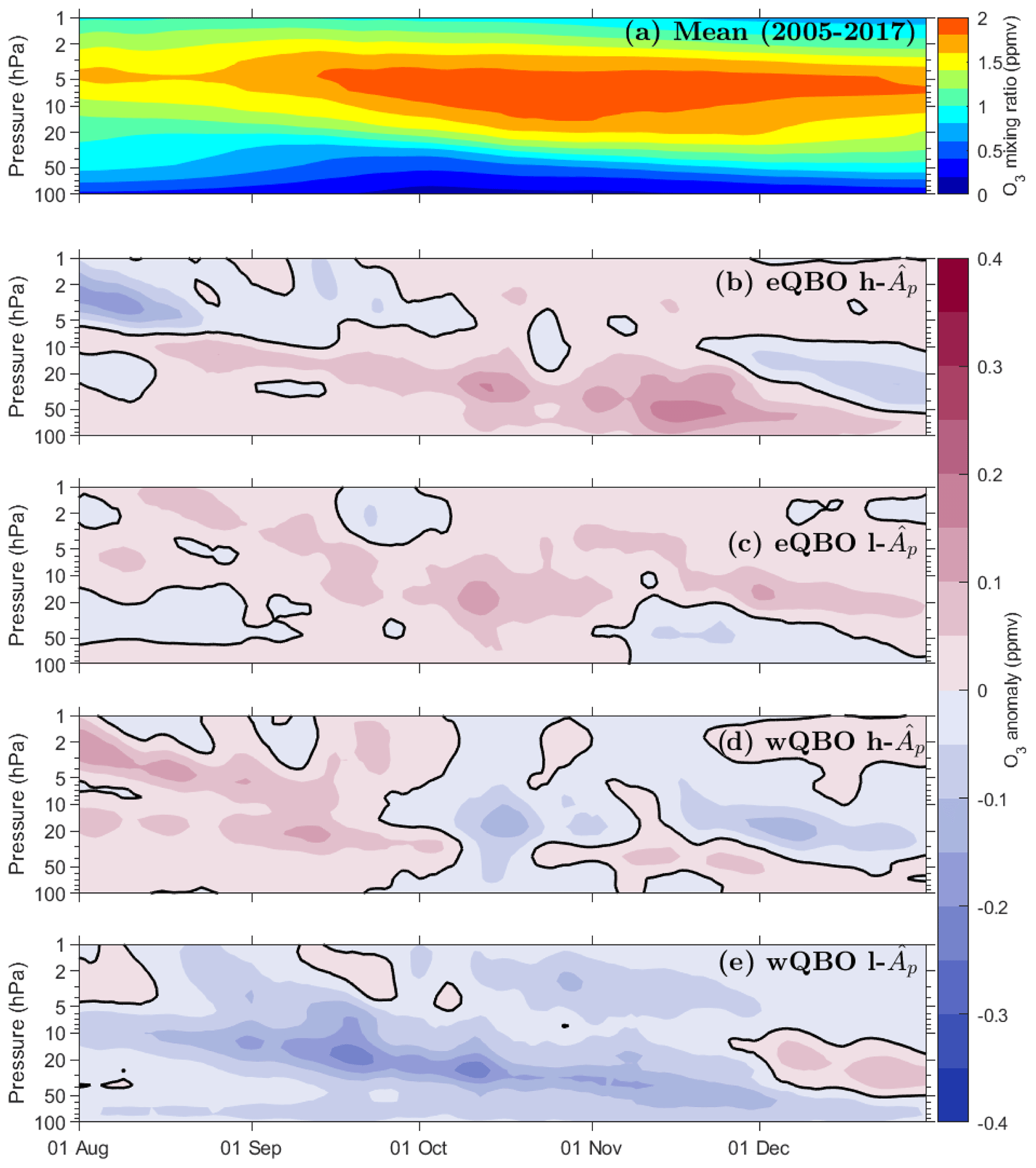
Figure 1 MLS profile ozone: (a) the composite zonal mean polar ozone (60–82^∘ S) mixing ratio for the study period (2005–2017) from early August until 31 December. The y axis is the pressure from 100 (∼18 km) to 1 hPa (∼50 km), and the x axis is time. The contour interval is 0.2 ppmv. (b) Anomaly from the mean for years with high $\widehat{\text{Ap}}$ and eQBO. The contour interval is 0.05 ppmv, and the black line indicates the zero contour. The axes are the same as for panel (a). Panels (c–e) are the same as panel (b) but for different combinations of $\widehat{\text{Ap}}$ and QBO phase (see individual panel labels). All data have been weighted by cos (latitude).

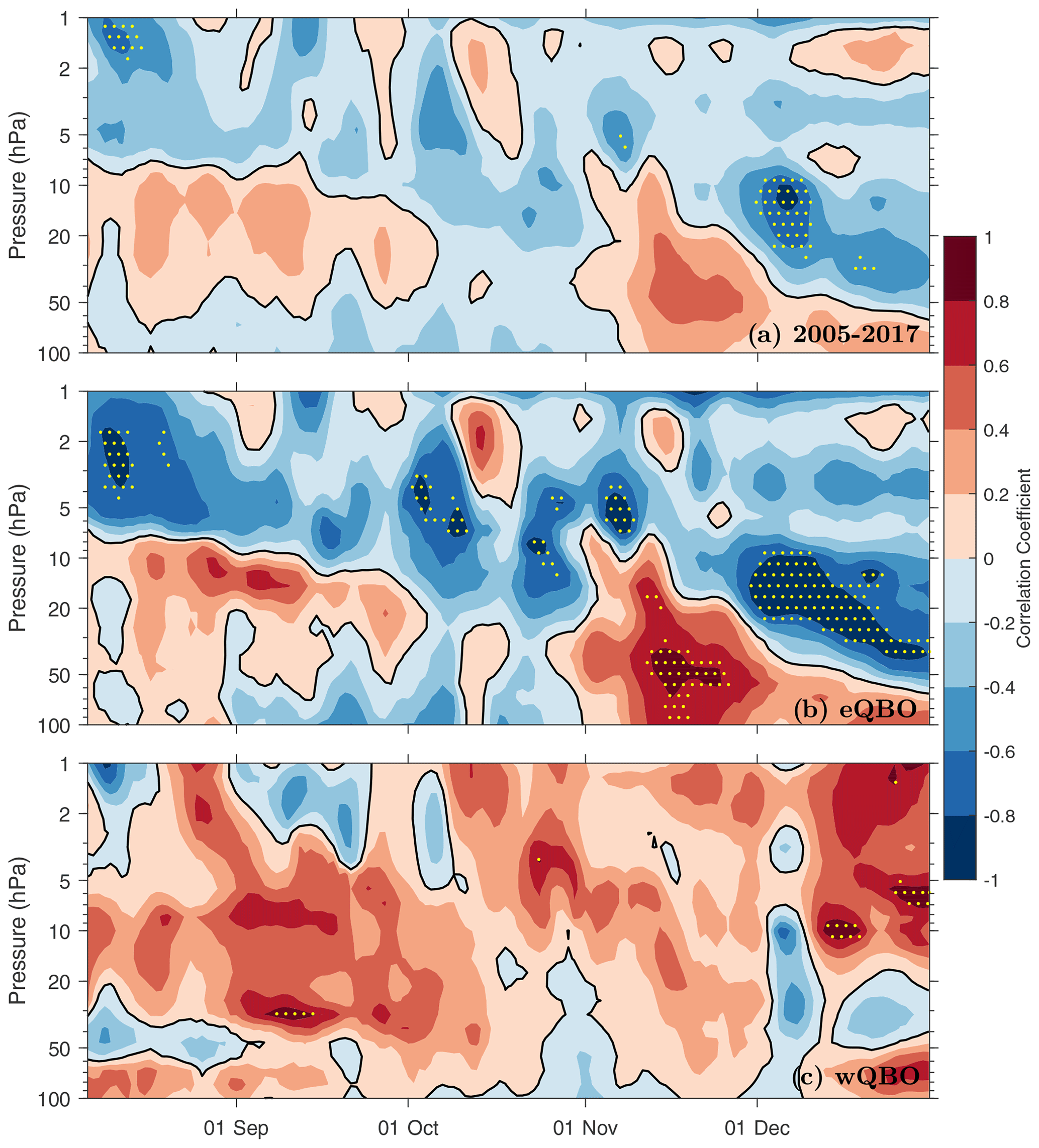
Figure 2 Correlation between the area-weighted polar (60–82^∘ S) MLS ozone mixing ratio and $\widehat{\text{Ap}}$ for (a) all years of the study, (b) eQBO years, and (c) wQBO years. The y axis is pressure (in hPa), and the x axis is time from the beginning of August until the end of December. Contours show the correlation coefficient with a 0.2 interval (black contour for zero), and stippling indicates statistical significance (p<0.05).

The above analysis indicates increases in ozone associated with high $\widehat{\text{Ap}}$ and, thus, high EPP, while also finding ozone decreases associated with the westerly phase of the QBO. We now look to see if the ozone increases linked to $\widehat{\text{Ap}}$ are correlated with $\widehat{\text{Ap}}$ levels and how this is modulated by the QBO phase. This is presented in Fig. 2 for all years (panel a), eQBO years (panel b), and wQBO years (panel c). There is significant anti-correlation ($\mathit{\rho }\sim -\mathrm{0.4}$ to −0.6) in the upper stratosphere around 2 hPa in panels a and b. This suggests that increases in $\widehat{\text{Ap}}$ indeed result in ozone loss in this area, particularly during eQBO. These ozone reductions are consistent with O₃ loss due to the EPP-NO_x descending in the polar vortex, as the pattern of descending significant negative correlation is consistent with the reported descending EPP-NO_x “tongue” (see e.g. Funke et al., 2014a). However, for eQBO conditions (Fig. 2b), the correlation pattern, which descends in time, is accompanied by a strong positive correlation (ρ>0.6) below ∼10 hPa in November. This indicates that EPP in eQBO years also contributes to ozone increases. At this time both Fig. a and b show positive correlation in the middle and lower stratosphere, although this is only statistically significant during eQBO years. We note that the positive correlation pattern does appear earlier and seems to descend with the negative pattern, but the positive correlation does not become statistically significant until November. A similar dipole pattern has previously been seen in model simulations with suggestions that it may be linked to chlorine and bromine chemistry (Jackman et al., 2009; Andersson et al., 2018). Our results here seem to suggest that increased $\widehat{\text{Ap}}$ results in ozone enhancement in November and that eQBO strengthens this relationship. There is little consistent correlation present in Fig. 2c; thus, there is no clear relation between polar springtime ozone profile variability and $\widehat{\text{Ap}}$ in wQBO years.

3.2 OMI column observations

We now repeat the analysis for the daily OMI total ozone column, instead of profile measurements. This is to verify whether the changes in ozone associated with EPP and the QBO are detectable in the ozone total column. While we lose the information contained in vertical profiles, we gain higher horizontal resolution. Note that the OMI data with 0.25^∘ gridding has been averaged here over 1^∘ latitude bins.

The composite 3 d running mean O₃ column from 2005 to 2017 is presented in Fig. 3a. The figure shows zonal mean ozone for each latitude poleward of 50^∘ S in 1^∘ bins as spring progresses from early August to the end of the December. Note that (1) no area weighting is required here; and (2) there are no data for the polar night, as OMI O₃ is measured with backscattered solar radiation. A key feature of Fig. 3a is the formation of the ozone hole in the springtime, with minimum ozone values of less than 150 DU in late September–early October at the pole. Figure 3b–e show the composite anomaly from the mean (panel a) for the same combinations of QBO phase and $\widehat{\text{Ap}}$ as before. Figure 3b corresponds to the anomaly for eQBO and h-$\widehat{\text{Ap}}$ years. In this case, the anomaly is almost entirely positive, with the largest values (>80 DU) occurring in mid-November. This implies that the combination of high $\widehat{\text{Ap}}$ and eQBO results in increased ozone throughout the springtime but especially in November. Figure 3c (eQBO, low $\widehat{\text{Ap}}$) is slightly more variable, especially in early spring. The easterly QBO appears to drive a positive ozone anomaly in October (as this appears in both eQBO panels); however, the sign of the anomaly changes in November, which seems to imply that low $\widehat{\text{Ap}}$ results in O₃ decreases (up to $\sim -\mathrm{50}$ DU) in November. Figure 3d (wQBO, high $\widehat{\text{Ap}}$) is again variable throughout early spring, with positive anomalies mainly present at highest polar latitudes. As in Fig. 3b for the eQBO, the positive anomaly (up to $\sim +\mathrm{50}$ DU) in November for the wQBO may be an indication that high $\widehat{\text{Ap}}$ is linked to ozone increases at this time. Lastly, Fig. 3e (wQBO, low $\widehat{\text{Ap}}$) shows a consistent negative anomaly: low $\widehat{\text{Ap}}$ in wQBO years results in an anomalously low ozone column ($\sim -\mathrm{40}$–50 DU) throughout spring. These column ozone results are consistent with the MLS ozone profile anomalies below 20 hPa (Fig. 1): in October and November, the combination of high $\widehat{\text{Ap}}$ and eQBO results in anomalously high ozone, whereas low $\widehat{\text{Ap}}$ and wQBO results in anomalously low ozone.

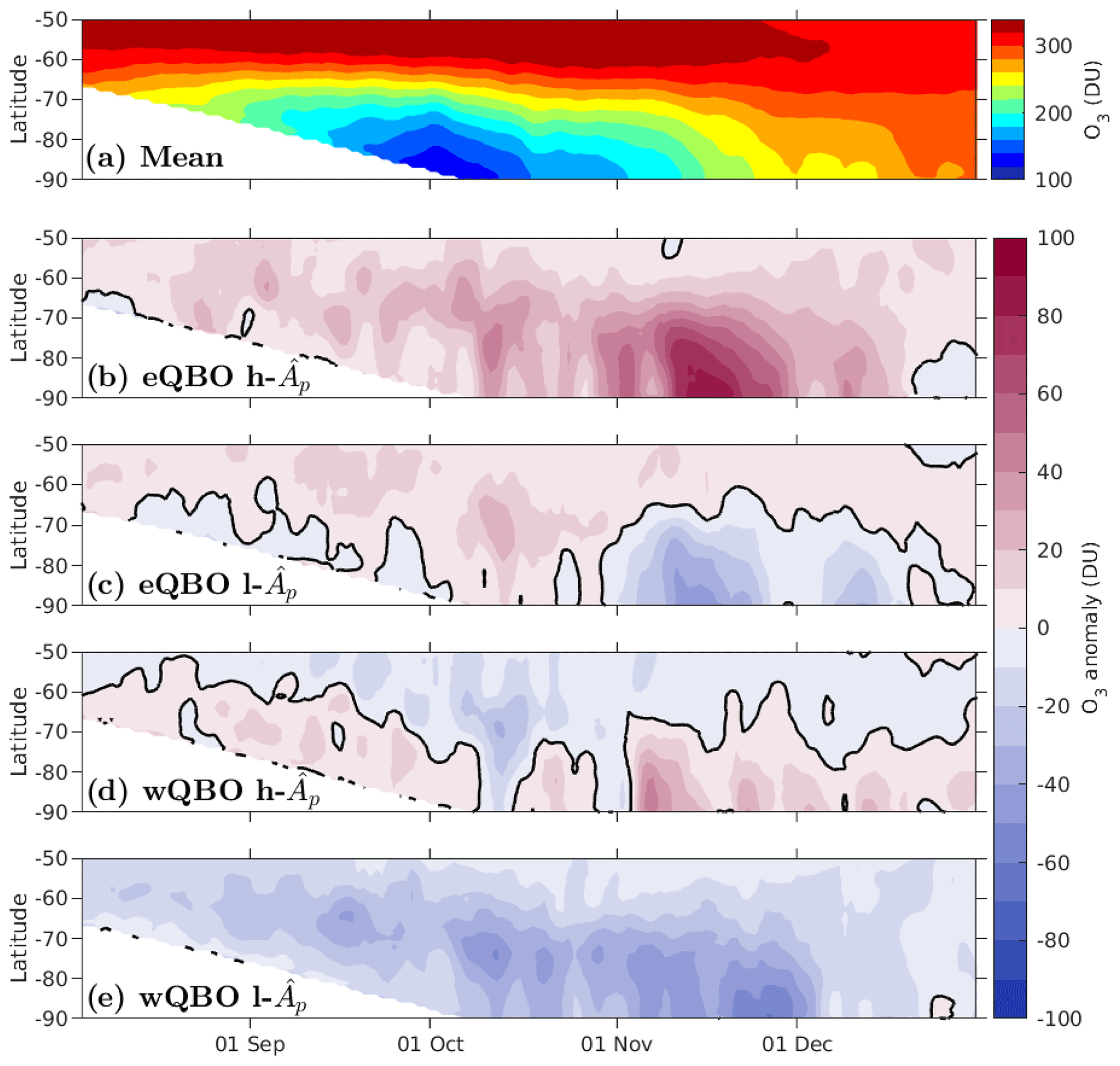
Figure 3 OMI ozone column: (a) August–December 3 d running mean zonal mean column ozone from 2005 to 2017 for latitudes 50–90^∘ S in 1^∘ bins (contour interval is 25 DU). The y axis is latitude, and the x axis is time from the beginning of August until the end of December. (b) Composite anomaly from the mean in panel (a) for eQBO years with high $\widehat{\text{Ap}}$. The x and y axes are the same as panel (a), the contour interval is 10 DU, and the zero contour shown in black. Panels (c–e) are the same as panel (b) but for different combinations of QBO phase and $\widehat{\text{Ap}}$ (see individual panel labels).

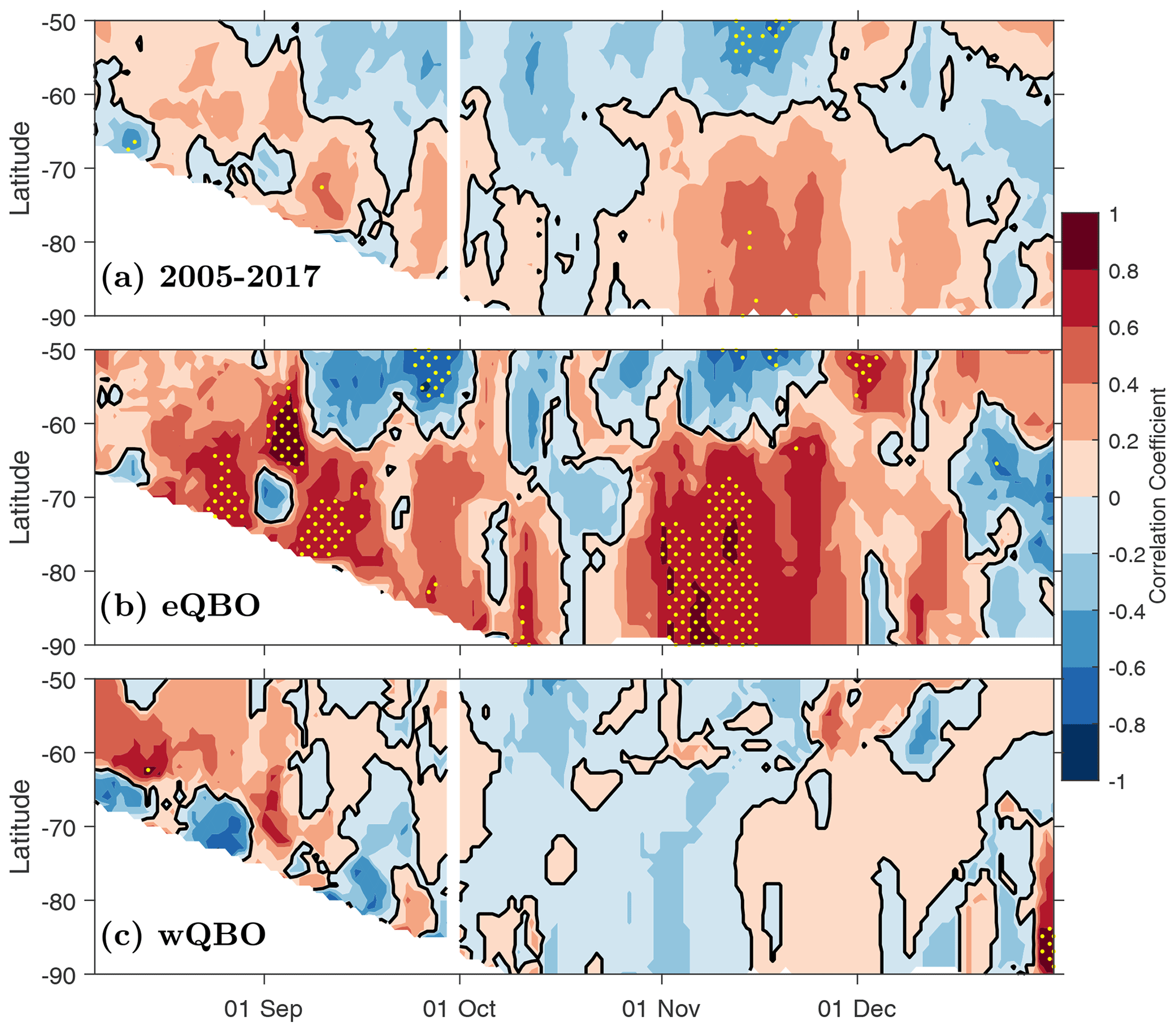
Figure 4 Correlation of zonal mean OMI O₃ and $\widehat{\text{Ap}}$ from August to December for latitudes 50–90^∘ S for (a) all years, (b) eQBO years, and (c) wQBO years. Contours represent the correlation coefficient, and the contour interval is 0.2 (the black line indicates the zero contour). Stippling indicates statistical significance at 95 %.

We now examine the correlation between ozone column (detrended) and $\widehat{\text{Ap}}$ level. This is shown in Fig. 4, with the panels representing all years (panel a), eQBO (panel b), and wQBO (panel c). Overall, the correlation is $\left|\mathit{\rho }\right|<\mathrm{0.6}$ everywhere, with little statistical significance, when all years are taken into account and no QBO-based binning is done. In Fig. 4b, for eQBO years, the correlation is positive poleward of 60^∘ S for almost all of spring. Areas of significant positive correlation (ρ≥0.6) occur throughout the period from August to October, and early November shows a consistent significant positive correlation. This agrees with Fig. 3: elevated $\widehat{\text{Ap}}$ results in ozone increases at high southern latitudes, and this is more prevalent in eQBO years. At lower latitudes, between 50 and 60^∘ S, there are patches of significant negative correlation. For wQBO years (Fig. 4c), the correlation is highly variable, with $\left|\mathit{\rho }\right|<\mathrm{0.4}$, and not significant. Any influence of EPP on the ozone column is generally weaker during wQBO years. This is consistent with Gordon et al. (2020), who reported significant correlation between stratospheric NO₂ column and EPP (as proxied by Ap) during eQBO years. Note that the missing values in late September are due to missing values in the time series. We have chosen not to calculate the correlation coefficient for these points so as not to be misleading about the number of years in each correlation calculation.

To quantify the effect that enhanced EPP has on the total ozone column in the Southern Hemisphere spring, Fig. 5a presents the average polar (60–90^∘ S) O₃ column in November as a function of $\widehat{\text{Ap}}$ for the preceding winter. Note that the ozone here is both cos (latitude) area weighted and detrended in order to account for reduced EESC. Red triangles represent eQBO years, and blue circles indicate wQBO years. The figure also shows best-fit lines, with red fitting eQBO years, blue fitting wQBO, and yellow fitting all data. There is a robust linear relationship between $\widehat{\text{Ap}}$ and ozone in eQBO years with the linear fit indicating an increase in the November total ozone column of 5.8 $\mathrm{DU}/\widehat{\text{Ap}}$, i.e. a 5.8 DU increase in the area-weighted O₃ per unit increase in $\widehat{\text{Ap}}$. The year-to-year variability in eQBO is in the range of 220–300 DU: 5.8 $\mathrm{DU}/\widehat{\text{Ap}}$ would correspond to about 2 % change in ozone per unit increase in $\widehat{\text{Ap}}$. Note that the wQBO year with detrended polar ozone less than 200 DU corresponds to the year 2015, when the ozone hole has been reported to be particularly large in area (Solomon et al., 2016). The 2 wQBO years with the highest detrended ozone columns correspond to the years 2013 and 2016, the latter of which presented a disruption in the QBO phase in February (Newman et al., 2016). The eQBO year with lowest ozone column corresponds to the year 2010. The QBO phase in 2010 changed during the Antarctic winter season from eQBO to wQBO, and this may have contributed to the low polar ozone amount in November.

Figure 5a accounted for the polar average with average 5.8 $\mathrm{DU}/\widehat{\text{Ap}}$. Figure 5b now shows the slope of the regression between $\widehat{\text{Ap}}$ and OMI ozone column in eQBO years for all points in the polar stratosphere with 1^∘ latitude resolution. Stippling is taken from Fig. 4b. We find that the slope is positive throughout November poleward of 60^∘ S. The maximum contribution of $\widehat{\text{Ap}}$ to column ozone occurs in mid-November poleward of 80^∘ S, with increases of greater than 15 $\mathrm{DU}/\widehat{\text{Ap}}$ – for example, up to a 15 DU increase in ozone south of 80^∘ S in mid-November per unit increase in $\widehat{\text{Ap}}$. These contributions occur simultaneously with significant correlation between the OMI O₃ column and $\widehat{\text{Ap}}$ in early to mid November.

Figure 5 (a) $\widehat{\text{Ap}}$ vs. OMI detrended polar ozone averaged over 60–90^∘ S with cos (latitude) weighting. Blue circles indicate years with a wQBO phase, and red triangles indicate those with a eQBO phase (eQBO and wQBO years as given in Table 1). The lines show the linear best fit with yellow fitting all data, blue fitting wQBO, and red fitting eQBO. Corresponding equations for these are included using the corresponding colours. Error bars are 2 times the standard error of the mean. (b) Evolution of the slope of the linear best fit between $\widehat{\text{Ap}}$ and OMI O₃ over November in the polar stratosphere in eQBO years. The y axis is latitude from 90 to 50^∘ S, and the x axis is the time from 1 to 30 November. The contour interval is 2.5 $\mathrm{DU}/\widehat{\text{Ap}}$. Stippling from Fig. 4b is superimposed as a reference to show where the OMI O₃ and $\widehat{\text{Ap}}$ correlation was found to be significant at 95 % or higher.

4 EPP indirect effect via chlorine species

Our results indicate ozone increases, both below 20 hPa in profile observations and in the total ozone column, with enhanced EPP. Traditionally, the long-term EPP effect on ozone has been considered to dominate via increased catalytic loss in NO_x cycles. Earlier works of Jackman et al. (2000) and Funke et al. (2014a) have, however, suggested there may be a more complex interplay, with NO_x interfering with ozone loss driving the halogen species ClO and BrO. To our knowledge, this effect has not been previously verified from observations.

Funke et al. (2014a) showed, using MIPAS observations, that in the Antarctic stratosphere, EPP-NO_y reaches altitudes as low as 22–25 km by September. They speculated on the effect that this EPP-NO_y might have on stratospheric ozone later in the spring, suggesting that EPP-NO_y could interfere with the buffering between ClO and ClONO₂ (via reaction (R5), that is changing the partitioning between ClO and ClONO₂ by conversion of ClO to inactive ClONO₂) and that “such EPP-induced buffering of ClO could even outweigh the ozone loss by EPP-NO_x, resulting in a net reduction of the Antarctic chemical ozone loss” (Funke et al., 2014a). Gordon et al. (2020) provided additional evidence for the sustained descent of EPP-NO_x, further suggesting that the phase of the QBO during the winter months plays a role in NO_x descent. Here, we found ozone increases under the same conditions. Motivated by the hypothesis of Funke et al. (2014a), we will now explore the mechanism they proposed: that EPP-NO_x modulates the amount of active chlorine in the springtime, but we will also account for the phase of the QBO.

4.1 MLS ClO observations

First, we investigate the composite mean ClO and the ClO anomaly from MLS observations. This is done for years with different combinations of $\widehat{\text{Ap}}$ and QBO phase as before and is presented in Fig. 6. Figure 6a illustrates the composite mean ClO averaged over 60–82^∘ S. Large amounts of ClO are activated in the lower stratosphere in the early spring (50–20 hPa, August through late September). This is followed by a large reduction in the ClO mixing ratio, due to deactivation of chlorine with the reformation of its reservoirs (von Clarmann, 2013). Note that values below zero are a result of the known negative bias in MLS ClO. The split panels (Fig. 6b–e) show the composite anomaly for different combinations of $\widehat{\text{Ap}}$ and QBO phase. As the abundance of ClO in the stratosphere changes dramatically throughout spring, each panel is divided into two, with the corresponding scale for each half indicated by the colour bar at the bottom of the columns. Note that the anomaly (regardless of the sign) in all panels appears to go from being contained in the upper or middle stratosphere in early spring (i.e. the left column) to a signal propagating down into the lower stratosphere in late spring (the right column). The descending anomalies are opposite for high and low levels of $\widehat{\text{Ap}}$: the ClO anomaly is negative (positive) for high (low) $\widehat{\text{Ap}}$ levels. Hence, high-$\widehat{\text{Ap}}$ years with negative ClO anomaly would indicate that EPP is associated with ClO decreases (−0.0050 to −0.0125 ppbv). This supports the above hypothesis that in years with high $\widehat{\text{Ap}}$ and, therefore, more EPP-NO_x, we should find reduced ClO, as enhanced NO₂ drives ClO to its ClONO₂ reservoir. The downward-propagating signal closely resembles the typical descent pattern of EPP-NO_x (see e.g. Funke et al., 2014a). Looking earlier in the season (left column), the descending anomalies can be traced up to the 5 hPa level. In the lower stratosphere in early spring, the anomalies generally appear to be more linked to the phase of the QBO with eQBO (wQBO) conditions leading to a reduction (enhancement) of ClO ($\sim \mp \mathrm{0.02}$ ppbv).

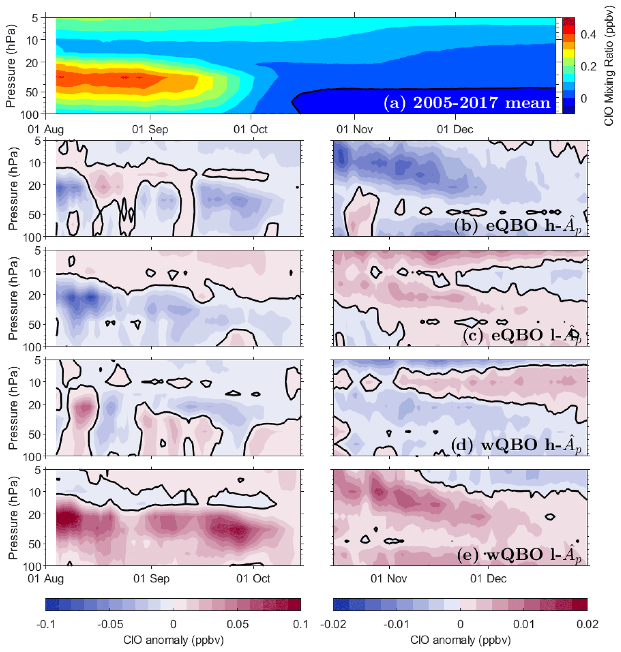
Figure 6 (a) Polar (60–82^∘ S, area-weighted) daytime MLS ClO composite mean over the 2005–2017 period. The contour interval is 0.05 ppbv. The y axis is the pressure from 100 to 5 hPa, and the x axis is the time from 1 August to the end of December. (b–e) The anomaly from the mean for (b) eQBO years and high $\widehat{\text{Ap}}$, (c) eQBO years and low $\widehat{\text{Ap}}$, (d) wQBO years and high $\widehat{\text{Ap}}$, and (e) wQBO years and low $\widehat{\text{Ap}}$. Due to the large change in ClO levels taking place in October, the left column presents the anomaly from 1 August to 15 October (contour interval of 0.01 ppbv), and the right column continues from 15 October to the end of December (contour interval of 0.0025 ppbv). The black line indicates the zero contour.

The correlation of MLS ClO and $\widehat{\text{Ap}}$ is presented in Fig. 7, in the same format as Fig. 2. Figure 7a (all years) and b (eQBO years) now show a similar downward-propagating anti-correlation, starting from about 2 hPa in the beginning of August and reaching almost 50 hPa by November. This again agrees well with downward descent patterns of EPP-NO_x that are known to be occurring at this time (see e.g. Funke et al., 2014a; Gordon et al., 2020). ClO being anti-correlated with EPP-NO_x aligns with the hypothesis that EPP-NO_x acts to drive ClO to its reservoirs. Our results show that this is more prevalent in eQBO years ($\mathit{\rho }\le -\mathrm{0.8}$ with p≤0.05), with wQBO years showing little significance. We also find a small positive region of significant correlation in the lower stratosphere (∼70 hPa) in August. It is unlikely that any EPP-NO_x has descended to such altitudes at this time. This could be related to some other mechanism, but it will not be investigated further here. Figure 7c (wQBO years) does not have the same significant anti-correlation descending in the stratosphere, but it does show a weak negative correlation following approximately the same descent pattern. We note that there is also a significant anti-correlation in the upper stratosphere in November to December, which is also present Fig. 7a and b. This may be related to the EPP-NO_y that remains in the upper stratosphere (see Figure 11 of Funke et al., 2014a) while the bulk descends to lower stratosphere.

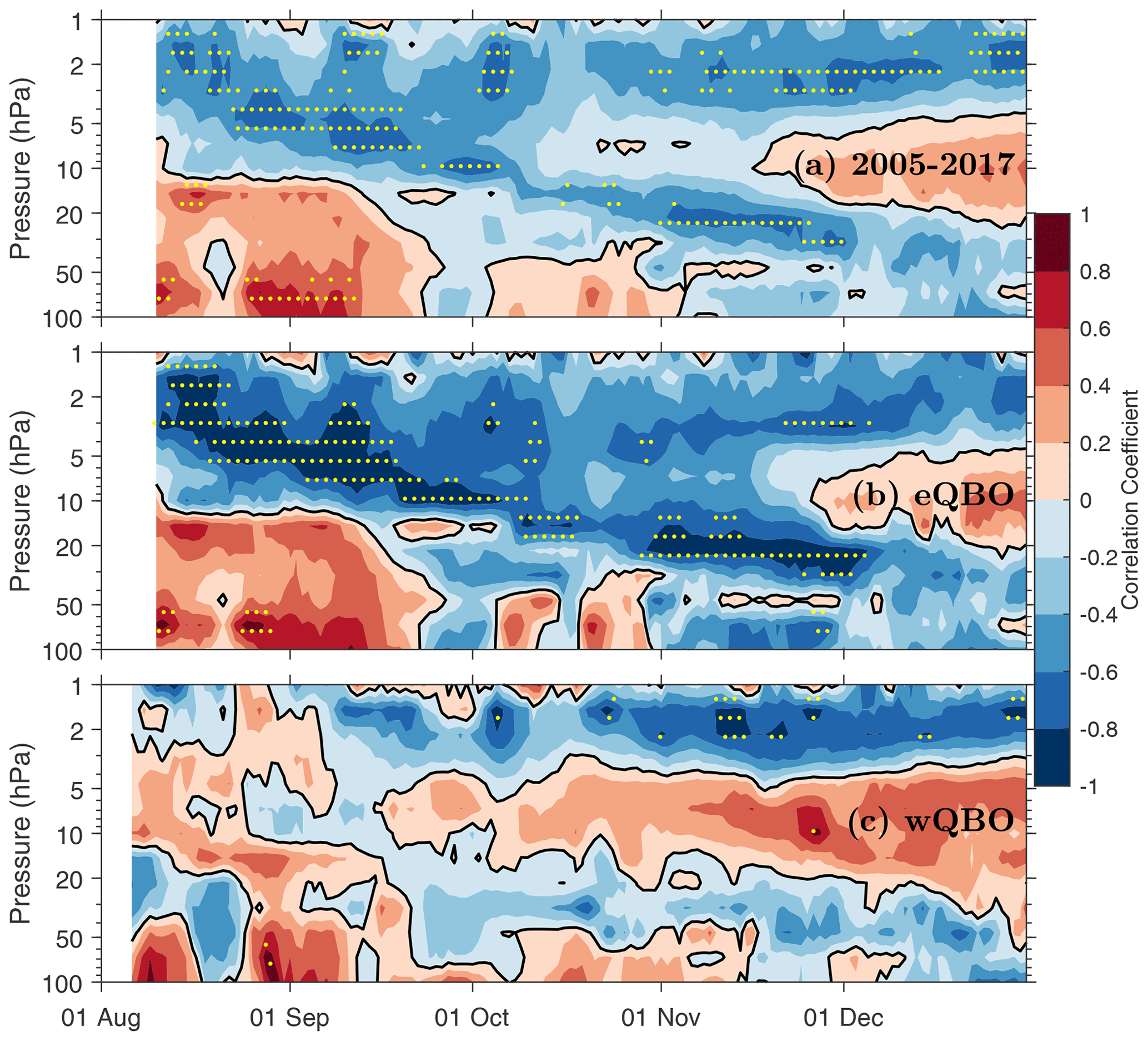
Figure 7 Correlation between $\widehat{\text{Ap}}$ and the detrended daytime MLS ClO averaged over 60–82^∘ S weighted by cos (latitude) for (a) all years, (b) eQBO years, and (c) wQBO years. The y axis is the pressure from 100 to 1 hPa, and the x axis is the time from 1 August to the end of December. The coloured contours show the correlation coefficient with a contour interval of 0.2, and the black line indicates the zero contour. Stippling indicates statistical significance (p≤0.05).

4.2 ClONO₂ observations from ACE-FTS and MIPAS

With the MLS observations providing credible evidence that stratospheric ClO is decreasing in the spring following elevated EPP during the polar winter, we now look for evidence of this being linked to enhanced levels of NO_x. The proposed buffering of ClO takes place via Reaction (R5) which converts the ClO to ClONO₂. This would remove both NO₂ and the active Cl_x from the catalytic ozone loss reactions, thereby resulting in overall ozone increase. To check whether ClONO₂ is increasing while ClO is decreasing, we analyse both ACE and MIPAS ClONO₂ in order to mitigate some of the coverage limitations of the observations.

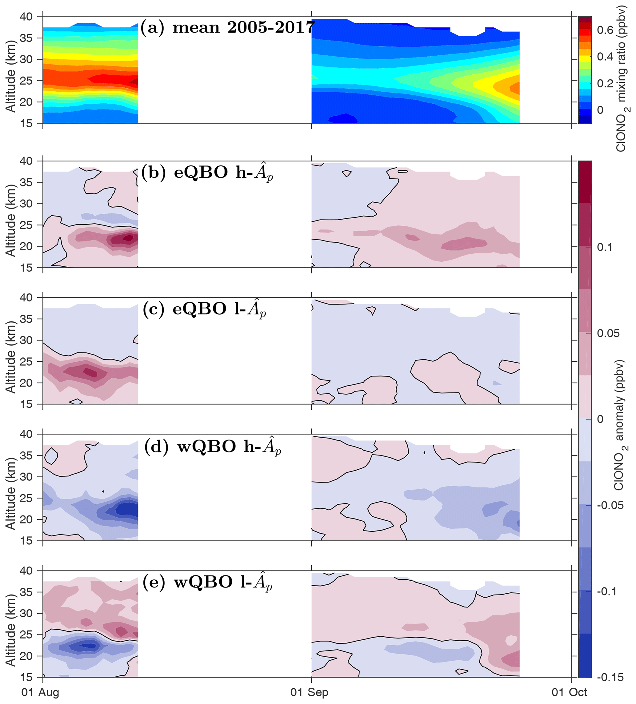
Figure 8 ACE-FTS ClONO₂: (a) the composite mean for the 2005–2017 period for area-weighted observations poleward of 60^∘ S. The y axis is the altitude from 15 to 40 km (∼120–2 hPa), and the x axis is the date from 1 August until 1 October. The contour interval is 0.1 ppbv. (b) The anomaly from the mean for eQBO years with high $\widehat{\text{Ap}}$, (c) eQBO years with low $\widehat{\text{Ap}}$, (d) wQBO years with high $\widehat{\text{Ap}}$, and (e) wQBO years with low $\widehat{\text{Ap}}$. The axes are the same as panel (a). The contour interval is 0.05 ppbv, and the black line shows the zero contour.

Figure 8 presents the mean ACE-FTS ClONO₂ as well as the anomalies for the different QBO phase and $\widehat{\text{Ap}}$ level combinations, as before. Figure 8a displays the composite mean of a 3 d running mean ClONO₂ from the beginning of August to the end of September averaged over 60–90^∘ S (weighted by cos (latitude)). The vertical scale here is altitude from 15 to 40 km (∼120–2 hPa). The orbit of ACE is designed to provide latitude patterns that repeat each year, allowing comparison between years, as yearly coverage is approximately the same. For the ACE-FTS and MIPAS analysis, we only include days where observations were recorded within 60–90^∘ S each year of the study. As the second half of August is not consistently observed by ACE every year, these measurements were not included. Note that ACE observations from August are taken at sunrise, and September observations are from sunset. Figure 8a highlights the large diurnal variation in ClONO₂: ClONO₂ is photolysed by UV radiation; thus, there is more in the atmosphere at sunrise than at sunset times (i.e. higher maximum in August than in September). The minimum that occurs below 25 km around the beginning of September is due to heterogeneous chemistry destroying ClONO₂ on the surface of PSCs (Brasseur and Solomon, 2005) while also inhibiting ClONO₂ formation, as PSCs remove NO₂ via denitrification in the lower stratosphere. ClONO₂ recovers around the time PSCs begin to disappear in late September. The anomalies for the combinations of $\widehat{\text{Ap}}$ and QBO phase (as shown in previous figures) are shown in Fig. 8b–e. The anomaly is variable in all cases, except for the lower stratosphere in August, which shows positive anomaly in August of the eQBO years (Fig. 8b, c) and negative anomaly in wQBO years (Fig. 8d, e). The anomalies in September are much smaller and mainly appear to show patterns in the lower stratosphere in mid to late September, once again showing positive anomaly in eQBO years and negative anomaly in wQBO years.

Figure 9 Correlation between $\widehat{\text{Ap}}$ and area-weighted ACE-FTS ClONO₂ poleward of 60^∘ S for (a) all years, (b) eQBO years, and (c) wQBO years. The y axis is the altitude from 15 to 40 km, and the x axis is the time from 1 August to the end of September. The coloured contours show the correlation coefficient with a contour interval of 0.2, and the black line shows the zero contour. Stippling indicates statistical significance.

The altitude-resolved correlation between ACE-FTS ClONO₂ and $\widehat{\text{Ap}}$ is shown in Fig. 9. Here, areas of consistent positive correlation (ρ≥0.6) occur in September in panel a (all years) and panel b (eQBO). These are statistically significant mostly in the middle and upper stratosphere in panel a and in the lower stratosphere in panel b. Figure 9a appears to support the hypothesis that ClO decreases are due to reactions forming ClONO₂. This is further supported by Fig. 9b which also shows that eQBO amplifies the signal. Figure 9c shows little consistent statistically significant correlation at this time.

Figure 10 (a) Composite mean of area-weighted MIPAS ClONO₂ averaged over 60–90^∘ S from 2006 to 2011. The y axis is the altitude range from 15 to 40 km (∼120–2 hPa), and the x axis is the time from early August until the end of December. The contour interval is 0.1 ppbv. (b) Anomaly for the composite mean of years with high $\widehat{\text{Ap}}$. The axes are the same as for panel (a), and the contour interval is 0.01 ppbv. Panel (c) is the same as panel (b) but for years with low $\widehat{\text{Ap}}$.

Due to the limited coverage in the spring, it is difficult to draw conclusive statements from ACE-FTS observations alone. Thus, we also analyse MIPAS ClONO₂ observations. Figure 10a presents the mean of ClONO₂ from MIPAS (we only use years 2006–2011 here) averaged over 60–90^∘ S, weighted by cos (latitude). Due to the relatively small number of years available, we only include regions that are observed every year; hence, white regions correspond to places that have missing coverage at some point from 2006 to 2011. Here, we see that ClONO₂ decreases throughout November in the lower stratosphere, below 30 km. Figure 10b and c show the anomaly for the composite mean of high-$\widehat{\text{Ap}}$ years and low-$\widehat{\text{Ap}}$ years respectively. Note that as the time series is different, the designation of high and low $\widehat{\text{Ap}}$ changes slightly: the mean $\widehat{\text{Ap}}$ for 2005–2011 is 6.6, and we take this as limit for low and high $\widehat{\text{Ap}}$. As this time period is shorter than that of OMI, MLS, and ACE-FTS, we do not sort for QBO here. Years with high $\widehat{\text{Ap}}$ (Fig. 10b) show a consistent positive anomaly (up to +0.06 ppbv) in the middle to upper stratosphere in early September, with this positive anomaly appearing to descend to around 23 km by late November–early December. This anomaly in late spring is consistent with the altitude range where we find ozone increasing with high $\widehat{\text{Ap}}$ (Fig. 2), although the anomaly is negative below ∼20 km. Similarly, we find descending negative anomaly in low-$\widehat{\text{Ap}}$ years (up to −0.06 ppbv). These results support the hypothesis that the O₃ increases in high-$\widehat{\text{Ap}}$ years result from enhanced NO₂ driving ClO to its ClONO₂ reservoir.

The altitude correlation between $\widehat{\text{Ap}}$ and MIPAS ClONO₂ is shown in Fig. 11. We again see a descending feature similar to those in Figs. 2 and 7. As this feature shows a positive (often significant) correlation (ρ>0.6), it is likely that this is again due to descending EPP-NO_x. Note also that as the ClONO₂ increases appear to coincide with ClO decreases, it is unlikely that this correlation is due to the decrease in EESC over this time period as that would result in each correlation having the same sign. Figure 11 shows that more ClONO₂ forms in high-$\widehat{\text{Ap}}$ years and in the same area as ClO decreases (Fig. 7), implying that the ClO depletion found earlier is due to ClONO₂ formation.

Figure 11 Correlation between $\widehat{\text{Ap}}$ and area-weighted polar MIPAS ClONO₂ for the 2006–2011 period. The y axis is the altitude from 15 to 40 km, and the x axis is the date from early August until the end of December. The coloured contours indicate the correlation coefficient with a contour interval of 0.2, and the black contour is the zero contour. Stippling indicates statistical significance.

Overall, these results suggest that the arrival of EPP-NO_x in the lower stratosphere by the late Antarctic springtime is contributing to faster conversion of active chlorine into reservoir species, which could bring about the end of the springtime ozone hole faster (as seen in the enhanced OMI total column ozone).

5 Conclusions

We have presented observational evidence that Antarctic springtime stratospheric ozone increases are associated with higher than average EPP during the preceding winter. Ozone increases due to the so-called EPP indirect effect had been previously suggested (Funke et al., 2014a), but, to our knowledge, this is the first time this has been shown in observations. Following the results of Gordon et al. (2020), we propose that this is due to EPP-NO_x which remains the lower stratosphere at least until November, having originally been transported from the mesosphere within the polar vortex. We were able to trace this descent pattern in observations of O₃, ClO, and ClONO₂, finding it matched that of the previously reported descent of EPP-NO_x (see e.g  Randall et al., 2006). Jackman et al. (2000) and Funke et al. (2014a) further proposed that should this NO_x reach the lower stratosphere (as shown by Gordon et al., 2020), it would react with ClO to form ClONO₂, preventing some of the NO_x- and Cl_x-driven catalytic ozone destruction. We examined polar ClO and ClONO₂ during the Antarctic spring and found decreases in ClO with consistent increases in ClONO₂ associated with above-average EPP. Thus, this provides direct observational evidence supporting the hypothesis of Jackman et al. (2000) and Funke et al. (2014a) that ozone loss may be decelerated in the Antarctic lower stratosphere following winters with high-EPP years due to excess NO_x accelerating ClO back to its reservoirs.

As Gordon et al. (2020) proposed in the context of Antarctic NO₂ column, we suggest that the reasons for the QBO modulating Antarctic ozone loss are also via its wave-forcing effect on the polar region (i.e. the Holton–Tan effect). Gordon et al. (2020) showed that eQBO years were more likely to have a warmer Antarctic vortex and proposed that this would lead to less denitrification in the lower stratosphere, resulting in a less suitable environment for PSC formation. As PSCs are crucial to springtime ozone loss in the lower stratosphere, we suggest that the inhibited PSC formation in eQBO years contributes to our findings that less chlorine is activated from reservoirs and, hence, less ozone loss in eQBO years, with EPP-NO_x contributing to increased ClONO₂ formation (see Reaction R5). This is similar to Sonkaew et al. (2013), who found that years with a warmer Arctic vortex resulted in less springtime ozone loss in the Northern Hemisphere. We suggest that this occurs in the Southern Hemisphere as well, but we also reinforce the important role played by EPP-NO_x.

Here, we again see the importance of the QBO: correlations of ozone with $\widehat{\text{Ap}}$ are higher (≥0.6 in OMI total ozone) and with more occurrences of statistical significance in eQBO years. This is in agreement with the higher correlation found in eQBO years between NO₂ and $\widehat{\text{Ap}}$ by Gordon et al. (2020). Our results further underline the appreciable effect of the QBO on the lower polar springtime stratosphere, and that the QBO phase should be accounted for in long-term studies of this region.

Our results have shown that the EPP indirect effect has indeed affected ozone over the period from 2005 to 2017, likely due to the interference of EPP-NO_x in Cl_x-catalysed ozone destruction. This period has also been marked by the continuing formation of the ozone hole every spring, although following the Montreal Protocol, the size of the ozone hole is generally decreasing with time (Solomon et al., 2016). The mechanism suggested in this paper (NO₂ buffering ClO) requires chlorine activation in the spring, but as chlorine loading in the polar stratosphere continues to decrease with the ban in CFC emissions, EPP-NO₂ will no longer hinder ozone depletion, likely instead becoming a major contributor. As ozone itself plays a vital role in both atmospheric chemistry and dynamics, this reinforces the importance of accounting for EPP in predicting the future of the polar middle atmosphere.