the Creative Commons Attribution 4.0 License.
the Creative Commons Attribution 4.0 License.
 | 24 Feb 2021
Technical note: Emission mapping of key sectors in Ho Chi Minh City, Vietnam, using satellite-derived urban land use data
Trang Thi Quynh Nguyen
Wataru Takeuchi
Prakhar Misra
Sachiko Hayashida
Emission inventories are important for both simulating pollutant concentrations and designing emission mitigation policies. Ho Chi Minh City (HCMC) is the biggest city in Vietnam but lacks an updated spatial emission inventory (EI). In this study, we propose a new approach to update and improve a comprehensive spatial EI for major short-lived climate pollutants (SLCPs) and greenhouse gases (GHGs) (SO2, NOx, CO, non-methane volatile organic compounds (NMVOCs), PM10, PM2.5, black carbon (BC), organic carbon (OC), NH3, CH4, N2O and CO2). Our originality is the use of satellite-derived urban land use morphological maps which allow spatial disaggregation of emissions. We investigated the possibility of using freely available coarse-resolution satellite-derived digital surface models (DSMs) to estimate building height. Building height is combined with urban built-up area classified from Landsat images and nighttime light data to generate annual urban morphological maps. With outstanding advantages of these remote sensing data, our novel method is expected to make a major improvement in comparison with conventional allocation methodologies such as those based on population data. A comparable and consistent local emission inventory (EI) for HCMC has been prepared, including three key sectors, as a successor of previous EIs. It provides annual emissions of transportation, manufacturing industries, and construction and residential sectors at 1 km resolution. The target years are from 2009 to 2016. We consider both Scope 1, all direct emissions from the activities occurring within the city, and Scope 2, that is indirect emissions from electricity purchased. The transportation sector was found to be the most dominant emission sector in HCMC followed by manufacturing industries and residential area, responsible for over 682 Gg CO, 84.8 Gg NOx, 20.4 Gg PM10 and 22 000 Gg CO2 emitted in 2016. Due to a sharp rise in vehicle population, CO, NOx, SO2 and CO2 traffic emissions show increases of 80 %, 160 %, 150 % and 103 % respectively between 2009 and 2016. Among five vehicle types, motorcycles contributed around 95 % to total CO emission, 14 % to total NOx emission and 50 %–60 % to CO2 emission. Heavy-duty vehicles are the biggest emission source of NOx, SO2 and particulate matter (PM) while personal cars are the largest contributors to NMVOCs and CO2. Electricity consumption accounts for the majority of emissions from manufacturing industries and residential sectors. We also found that Scope 2 emissions from manufacturing industries and residential areas in 2016 increased by 87 % and 45 %, respectively, in comparison with 2009. Spatial emission disaggregation reveals that emission hotspots are found in central business districts like Quan 1, Quan 4 and Quan 7, where emissions can be over 1900 times those estimated for suburban HCMC. Our estimates show relative agreement with several local inherent EIs, in terms of total amount of emission and sharing ratio among elements of EI. However, the big gap was observed when comparing with REASv2.1, a regional EI, which mainly applied national statistical data. This publication provides not only an approach for updating and improving the local EI but also a novel method of spatial allocation of emissions on the city scale using available data sources.
- Article
(2155 KB) - Full-text XML
-
Supplement
(364 KB) - BibTeX
- EndNote


Emission inventories (EIs) are key for identifying the source of pollutants. This is particularly true in Southeast Asia, where the rise of energy demands results in significant air quality and human health issues. A number of regional anthropogenic EIs exist to be used as input for atmospheric chemistry models and also to understand the long-term trends of emission levels in this area (Table 1). But only a few attempts have been made to understand the annual evolution of Asian emissions. REAS (Regional Emission inventory in ASia) is the first inventory to integrate time series of emission data for Asia on the basis of a consistent methodology. REASv2.1 was developed from REASv1.1 with the spatial resolution of gridded data improved to 0.25∘ × 0.25∘ and temporal resolution increased to monthly (Kurokawa et al., 2013). REASv3.1 was updated to 2015 and covers the longer historical time span from 1950–2015 (Kurokawa et al., 2020). These inventories were compiled on a regional scale with coarse resolutions and are no longer updated. They mainly applied national energy consumption data as activity data. Apart from countries having their own databases of emission factors (EFs) like China and Japan, EFs of other Asian countries were extracted from many sources, including previous Asian EIs and recent studies.

According to the Global Protocol for Community-Scale Greenhouse Gas Emission Inventories (GPC), urban areas are responsible for more than 70 % of global energy-related carbon dioxide emissions, and the achievement of emission reduction of the economy in the upcoming decades will depend mainly on cities. Thus, it is very important to develop an EI on the city scale. At the same time, a continuous historical EI could show the long-term evolution of emissions as a consequence of socio-economic development in cities. In response to these needs, the GPC establishes credible emission accounting and reporting practices that help cities to calculate and report community-scale greenhouse gases and develop their own historical EIs.
A research study by Yale University found that Vietnam's PM2.5 index ranked 170th out of 180 surveyed countries, and Vietnam is considered one of the 10 most polluted countries in the world in terms of air quality (Yale Center for Environmental Law and Policy, 2018). In urban areas like Hanoi and Ho Chi Minh City (HCMC), the situation has become worse because of the high intensity of anthropogenic activities. In the first quarter of 2018, the average PM2.5 concentrations measured in Hanoi and HCMC reached 63.2 and 37.2 µg m−3, respectively (GreenID, 2018). However, while air pollution levels in Hanoi exhibit strong seasonality and a dependence on meteorological factors, air quality in HCMC is mainly influenced by anthropogenic emissions occurring inside the city (GreenID, 2018). For these reasons, in this study, we focus on the annual emissions of HCMC, Vietnam.
In 2017, the first comprehensive greenhouse gas (GHG) inventory of HCMC was prepared for 2013, 2014 and 2015 with the assistance of the Japan International Cooperation Agency (JICA) under the Project to Support the Planning and Implementation of Nationally Appropriate Mitigation Actions in a Measurement, Reporting and Verification Manner (SPI-NAMA). According to their calculation, among five main anthropogenic sectors, transportation and stationary energy are the two most prominent emission sectors in HCMC, comprising 45 % and 46 % of the total, respectively. Within the stationary energy sector, manufacturing industries account for the highest portion (46 %), followed by residential buildings (33 %) (JICA, 2017a). Another EI was compiled to calculate emissions and forecast for 2025 and 2030 (Ho et al., 2019). This EI includes on-road emission sources, non-road mobile sources, area sources and biogenic sources. In addition to these comprehensive studies, several EIs were developed for HCMC but mainly focused on road traffic emission (Belalcazar, 2009; Ho, 2010; Oanh and Van, 2015; Le et al., 2018). These studies have a low level of consistency and inheritance from previous EIs. Also, with the rapid economic development in HCMC, the significant evolution of various emission sources is expected. As a result, it is important to compile a detailed and continuous local EI for this city.
With respect to grid allocation, spatial distribution of emissions is a crucial step to fulfill the requirements of gridded EI as input data for air quality modeling. Top-down EIs are often used as input data for modeling activities at the urban scale after downscaling (López-Aparicio et al., 2017). In a conventional way, other methodologies focus only on the disaggregation of transport emissions using traffic counts and road network data (Gómez et al., 2018). The spatial allocation of area source emissions is mainly based on rural, urban and total population data (Kurokawa et al., 2013, 2020). These approaches are not suitable for community-scale EIs that demand higher detail levels of both activity data and spatial disaggregation. In particular, it is not rational to use population data for spatial disaggregation of the industrial sector. Using these methodologies without consideration could lead to underestimation of emissions in urban centers and industrial zones as well as overestimation in residential zones (Saide et al., 2009). It is worth mentioning that these spatial proxies have a strong influence on simulations of air quality modeling, especially when the results are considered for policy making and planning options (Trombetti et al., 2018). Kühlwein et al. (2002) made comparisons among spatial distribution of EIs computed with different levels of information and concluded that a big source of uncertainty is encountered when only considering disaggregation using population. Trombetti et al. (2018) also conducted an inter-comparison of the main top-down EIs currently used for air quality modeling studies at the European level regarding downscaling approaches and choice of spatial proxies. Their finding is that the traditional proxies used for gridding residential emissions (e.g., population density) would not be any more relevant. A few studies used land use maps as a proxy for deriving spatial patterns of emissions (Saide et al., 2009). Today, remote-sensing information is a quite important source for land use and land cover modeling. The most prominent advantages of satellite images influencing the spatial allocation of emissions are the ability to collect information over large spatial areas and the ability to collect imagery of the same area of the Earth's surface at different periods in time. By imaging on a continuous basis at different times, it is possible to monitor the changes in land use on the community scale if the resolution of data is high enough. Moreover, data collected through remote sensing are analyzed at the laboratory, which minimizes the work that needs to be done on the field. Accordingly, in the context of spatially allocating emissions at a finer scale, remote sensing data are a quite promising approach that allows repetitive land use mapping in different study areas. In the case of HCMC, only a few attempts have been made to spatially disaggregate the emissions. Applying a similar method with previous works, the study of Ho (2010) provides the first emission maps for HCMC using the road network as an allocation factor for the transportation sector and population density as an allocation factor for the industrial and residential sectors.
In response to these needs, we developed an annual inventory, focusing on three key sectors: (1) transportation, (2) manufacturing industries and (3) residential buildings, using a higher detail level of activity data, local EFs for HCMC and a novel approach for grid allocation using remote sensing data. This local EI covers from 2009 to 2016 and includes emissions of the following species: SO2, NOx, CO, non-methane volatile organic compounds (NMVOCs), black carbon (BC), organic carbon (OC), CO2, NH3, CH4 and N2O, PM10 and PM2.5. As the successor of REASv2.1, this EI provides Asian anthropogenic emissions from 2000 to 2008. Moreover, this study inherits the statistics used in GHG emission inventories provided by JICA for 2013, 2014 and 2015. Both Scope 1, direct emissions from the activities occurring within the city, and Scope 2, indirect emissions from electricity purchased, are considered. Accordingly, this EI is the successor of REASv2.1 and the GHG emission inventory provided by JICA. In this study, only annual emissions are considered because air pollution levels in HCMC do not exhibit strong seasonality and a dependence on meteorological factors like in Hanoi (GreenID, 2018). The novelty of our work is the use of satellite-derived urban land use morphological maps which allow spatial disaggregation of emissions. Section 2 describes the methodology used in our EI to estimate emissions, including activity data, emission factors and spatial distribution of EI. Section 3, the results and discussion, covers four topics: (1) emissions from each sector, (2) Scope 1 and Scope 2 emissions, (3) spatial distribution, and (4) comparison with other inventories. Finally, the Monte Carlo method was applied to perform uncertainty analysis of estimated EIs. A summary and conclusion are given in Sects. 4 and 5.
2.1 Study location
HCMC is the most populous city in Vietnam with a population of 9 million as of 2019. Air quality in this city is mainly influenced by anthropogenic emissions occurring inside the city. In other words, the relative independence of the situation in this city of other adjacent sources facilitates compilation of a local EI. Also, the local emissions are dominant sources of pollution (GreenID, 2018). Figure 1 shows the inventory domain of our EI.
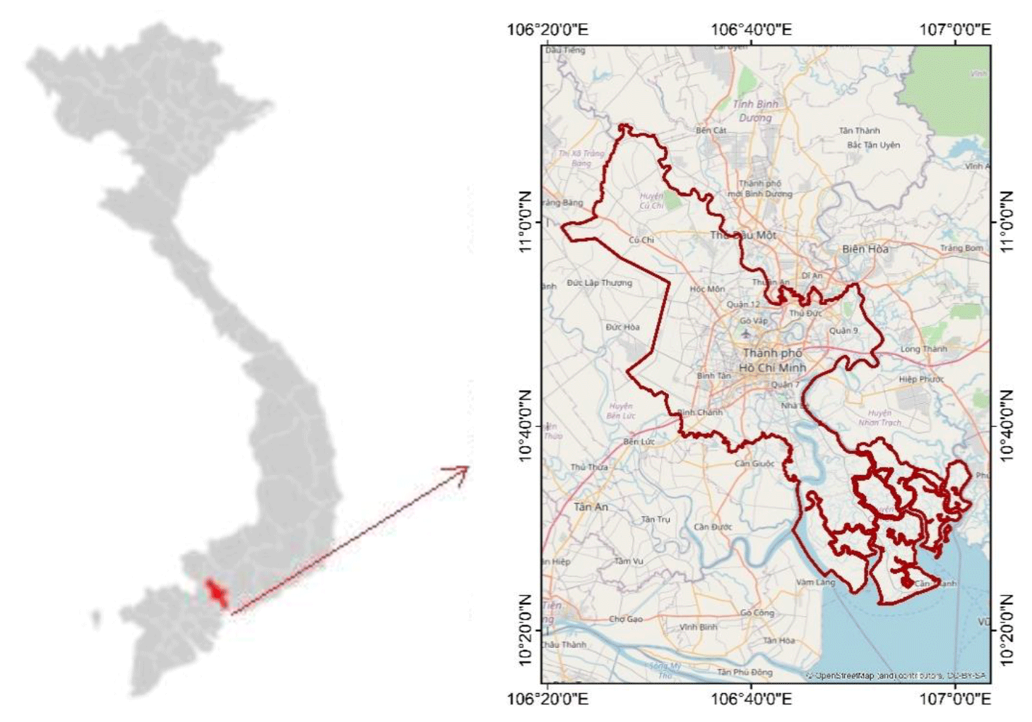
Figure 1Ho Chi Minh City – inventory domain of our EI (© OpenStreetMap contributors 2019. Distributed under a Creative Commons BY-SA License).
2.2 General description
Table 2 summarizes the general information of our EI that includes nine major air pollutants and three greenhouse gases, as a successor of REASv2.1: SO2, NOx, CO, non-methane volatile organic compounds (NMVOCs), black carbon (BC), organic carbon (OC), CO2, NH3, CH4, N2O, PM10 and PM2.5. The target years are from 2009 to 2016, to continue the period covered by REASv2.1. Source categories considered in this inventory are basically the same as the GHG EI that was compiled based on the guidelines of GPC. But here we focus on only three dominant sectors defined by the GHG EI developed by JICA (2017b): (1) transportation, (2) manufacturing industries and (3) residential buildings. The spatial resolution is improved to 1 km to provide detailed grid nets for atmospheric chemistry models and emission maps for local government and decision makers. In addition, we collected more city-specific activity data and local emission factors (EFs) from recent studies of EIs for Asian countries (see Sect. 2.3).

2.3 Basic methodology
2.3.1 Transportation emission
Figure 2a shows the flow diagram for estimating emissions from road transport. On-road vehicles were classified as motorcycles (MCs), taxis, cars, buses and heavy-duty vehicles (trucks), each of which includes gasoline and diesel vehicles. We calculated annual hot emissions based on the annual number of registered vehicles, average daily vehicle mileage traveled, and emission factors for each vehicle type with the following equation:
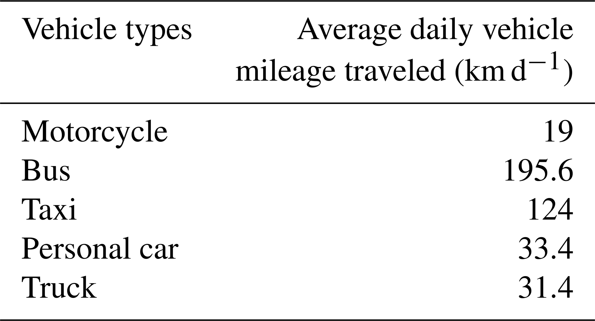
where i represents vehicle types, daily VKT is the average daily vehicle kilometers traveled for vehicle type i (km d−1), VPi is the population of vehicle type i and EFi is the hot emission factor of vehicle type i. The daily VKTs of each vehicle type in HCMC (2013) were extracted from the study of Oanh and Van (2015) and were assumed to be constant over the years (Table 3).
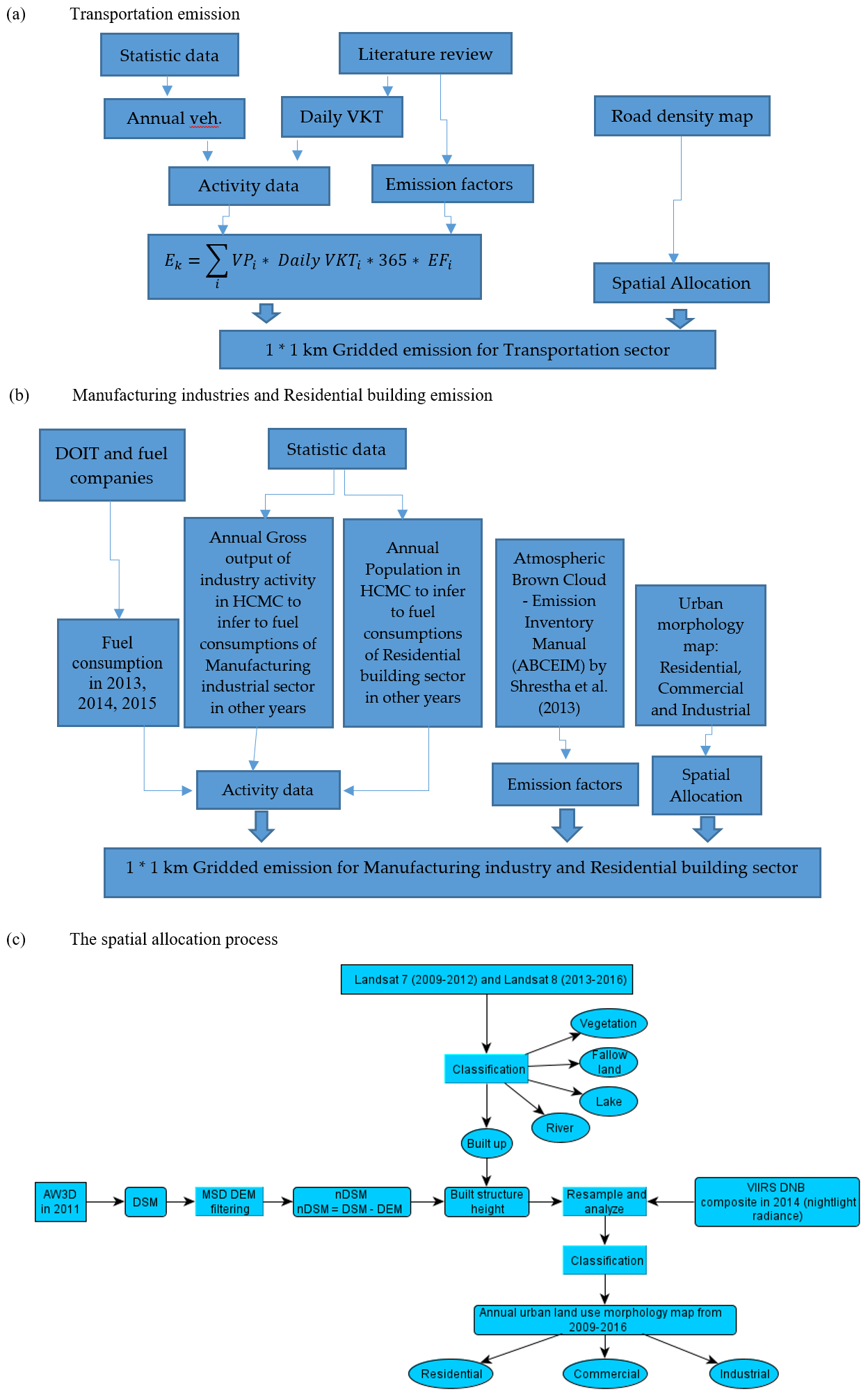
Figure 2Schematic flow diagrams showing estimation of emissions from (a) transportation sources, (b) manufacturing industry sources and residential building sources as well as (c) the spatial allocation process.
Table 3Average daily vehicle kilometers traveled of vehicle types in HCMC (Oanh and Van, 2015).
The vehicle population data were synthesized by different data sources, such as the statistic of the transport department of HCMC and previous studies about vehicle emissions in HCMC. However, the annual number of registered vehicles in some types was missing, such as population of trucks and buses over the years. The number of trucks was calculated based on the data in 2013 (Oanh and Van, 2015) and proportionally estimated for other years based on annual volume of freight carried that was provided by the HCMC Statistical Yearbook. The bus population and the taxi population in 2015 and 2016 were proportional to the number of cars (Table 4).
Table 4Number of registered vehicles by type in HCMC over the years.
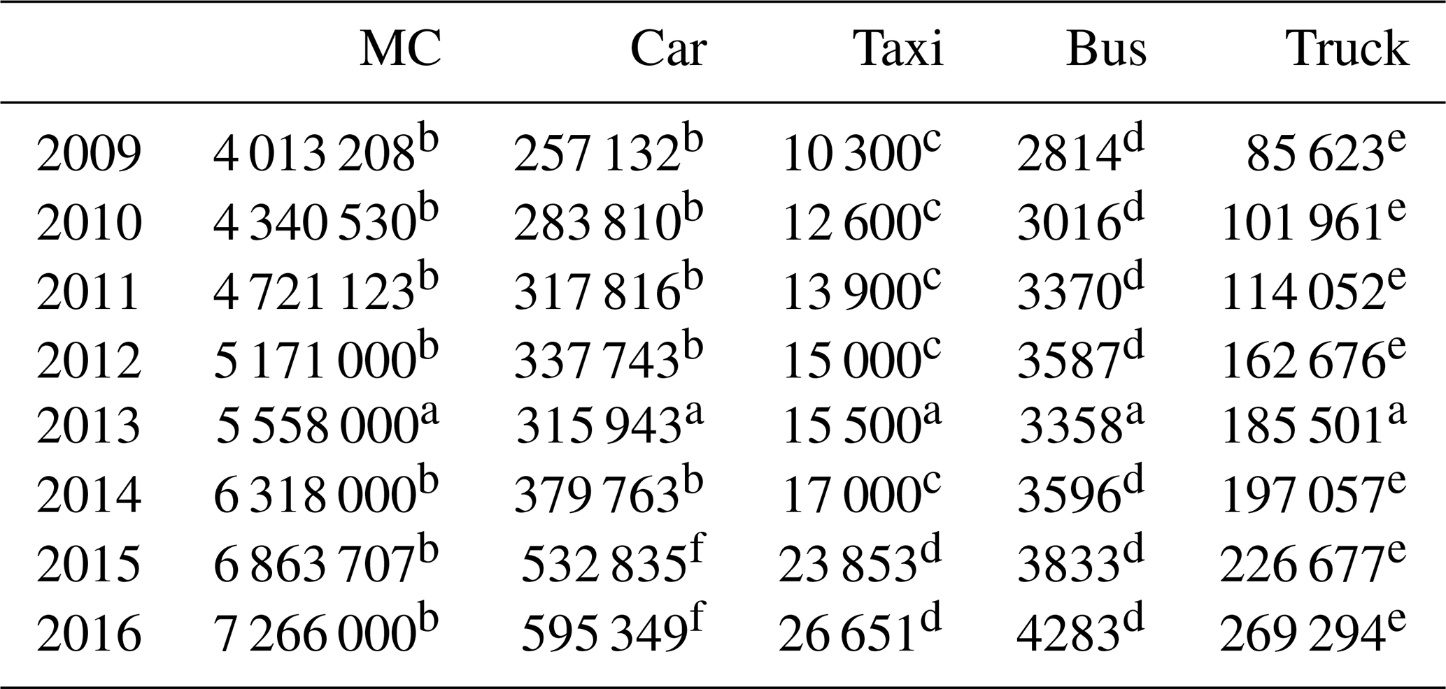
a Oanh and Van (2015). b Statistical data provided by the Transport Department of HCMC. c JICA, Report on Ho Chi Minh City – Osaka City Cooperation Project for Developing Low Carbon City (2016). d Proportional estimation basing on number of cars. e Proportional estimation based on annual volume of freight carried that was provided by the HCMC Statistical Yearbook. f Le and Leung (2018).
Cold emissions from road transport were included for NOx, CO, PM10, PM2.5, BC, OC and NMVOCs by the following equation:
Cold emissions were adjusted according to hot emissions using the fraction of distance traveled driven with a cold engine or with the catalyst operating below the light-off temperature (βi) and the correction factor of EFhot for cold-start emissions (Fi) The parameters β and F are functions of average monthly temperature. Equations for β and F and related parameters were taken from the EMEP/EEA EI guidebook 2009 (EEA, 2009). Monthly average surface temperatures in HCMC were adopted from https://www.weather-atlas.com/ (last access: 25 November 2018).
The EFs were extracted from seven different studies conducted in Hanoi and China (Table 5), covering 12 pollutant species. In Eq. (1), EFs and daily VKTs of each vehicle type were assumed to be constant over the years. This usage of constant EFs and daily VKTs is a result of limited availability of public data. Therefore, the annual emissions were mainly driven by vehicle populations.
Table 5The emission factors (g km−1 per vehicle) from literature review.

a Trang et al. (2015, study in Hanoi). b Hung et al. (2014, study in Hanoi). c Oanh et al. (2012, study in Hanoi). d He et al. (2014, study in China). e Belalcazar et al. (2009) and Ho et al. (2006) (studies in HCMC). f Cai et al. (2013, Updated Emission Factors of Air Pollutants from Vehicle Operations in GREET Using MOVES). g EMEP/EEA air pollutant emission inventory guidebook (2016, updated in 2018).
2.3.2 Manufacturing industry emissions
Figure 2b shows the basic procedure to estimate emissions from the manufacturing industry sector. It focuses on fuel-consumption-based emissions which are considered to be Scope 1 emissions. Scope 1 refers to all direct emissions from sources located within the city boundary. In addition, this study will calculate Scope 2 electricity-consumption-based emissions separately (Sect. 2.3.4). Emissions from fuel combustion were calculated from the following equation, similar to the one applied in REASv2.1:
where E is emissions from fuel consumption of manufacturing activities, i is fuel type, A is fuel consumption, EFi is unabated emission factor of each combustion species and Ri is reduction efficiency of the control device. In the case of SO2, the emission factor was estimated from the following equation:
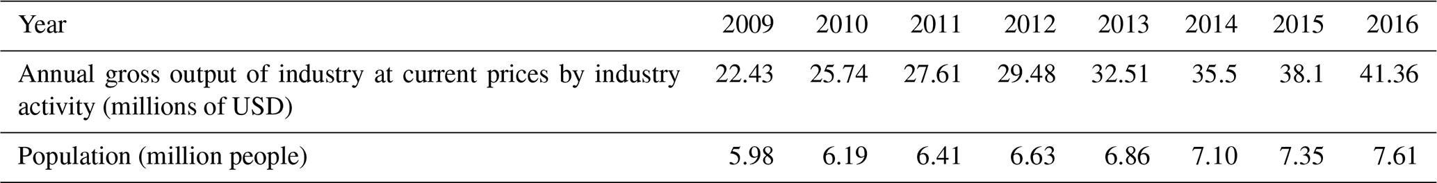
where is emissions of SO2 for each fuel type, Si is sulfur content of fuel and SR is sulfur retention in ash. The total fuel consumption in HCMC (2013, 2014, 2015) with the ratio of final fuel consumption by sub-sector and fuel type (Table 6) was provided in the GHG EI compiled by JICA (2017a). Based on this GHG EI, the annual fuel consumption of manufacturing industry and residential sectors, including gasoline, diesel, heavy oil, kerosene, liquefied petroleum gas (LPG) and natural gas, can be estimated for 3 years: 2013, 2014 and 2015. The fuel consumption of the manufacturing industry sector in 5 other years (2009 to 2012 and 2016) was proportionally calculated using annual gross output of industry at current prices by industry activity in HCMC, provided by the HCMC Statistical Yearbook (Table 8) with the assumption that there is a linear relationship between fuel consumption of the manufacturing industry sector and gross output of industry. Unabated emission factors, reduction efficiencies of each pollutant species, sulfur content of fuel and sulfur retention in ash were adopted from the compiled database presented in the Atmospheric Brown Clouds: Emission Inventory Manual (ABCEIM) by Shrestha et al. (2013). ABCEIM has included EFs from several databases as well as available measurement data reported for various sources in Asia (Table 7).
Table 6Annual fuel consumption in HCMC (2013, 2014, 2015) and ratio of final fuel consumption by sub-sector (manufacturing industry and residential sectors) and fuel type in Vietnam in 2014 provided by JICA (2017a).

Table 7Emission factors for manufacturing industry and construction (a) and residential (b) sectors from the compiled database provided by the Atmospheric Brown Clouds – Emission Inventory Manual (ABCEIM) by Shrestha et al. (2013). PM2.5 and PM10 were merged into PM for the residential sector in this database (except SO2) (unit: kg TJ−1).
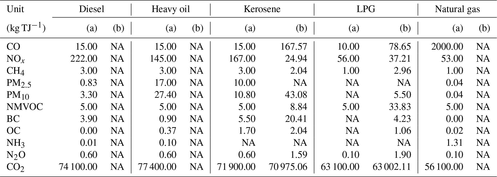
NA – not available.
Table 8Annual gross output of industry at current prices by industry activity in HCMC and population of HCMC over the years provided by the HCMC Statistical Yearbook.
2.3.3 Residential emission
Figure 2b shows the flow diagram for estimating emissions from the residential sector. This sector covers all fuel combustion activities in households, including domestic cooking and use of fireplaces. Kerosene, liquefied petroleum gas (LPG) and natural gas are used for cooking, while kerosene is used for lighting in the residential sector in many regions. Coal and biomass fuels such as wood are used mostly for domestic cooking and heating stoves in rural areas. Similar to the manufacturing industry sector, the annual emissions from the residential sector were calculated using Eqs. (3) and (4). Fuel consumption in 2013, 2014 and 2015 was provided by GHG EI compiled by JICA (2017a) (Table 6). The fuel consumption in other years was proportionally calculated using population provided by the HCMC Statistical Yearbook (Table 8) with the assumption that there is a linear relationship between fuel consumption of the residential sector and population of the city.
The uncontrolled emission factors and reduction efficiencies for the residential sector, sulfur content of fuel and sulfur retention in ash were adopted from ABCEIM by Shrestha et al. (2013) (Table 7).
2.3.4 Emissions from electricity consumption
Apart from Scope 1 emissions, this study also considered CO2 Scope 2 emissions that are from purchased energy generated upstream from the city, mainly electricity. Consumption-based emissions encompass those emissions produced by consumption within those same boundaries, regardless of the origin of those emissions. Local governments often include Scope 2 emissions when they do not have electric generating plants within their boundaries but still wish to evaluate the impacts of electricity use in the community. CO2 emissions from electricity consumption of manufacturing industries and residential sectors were calculated from the simple equation
where E is emissions from electricity consumption, A is activity data which here is the amount of electricity consumption from each sector and EFelectricity is grid emission factor, specific for each region. In GHG EI compiled by JICA, the electricity consumption in 2013, 2014 and 2015 by sub-sectors was collected from Vietnam Electricity (EVN) using data collection forms. The electricity consumption consists of five sub-sectors (residential buildings, commercial and institutional buildings and facilities, manufacturing industries and construction, energy industries and agriculture, and forestry and fishing activities) (Table 9). This value includes emissions from both consumption of grid-supplied energy consumed within the city boundary and transmission and distribution loss from grid-supplied energy.
Table 9Electricity consumption of manufacturing industry and construction and residential sectors and grid emission factors in HCMC (2013, 2014, 2015), provided by Electricity of Vietnam (EVN).

The significant linear relationships during 2013–2015 between electricity consumption of the industry sector and residential sector with annual gross output of industry and annual population were found (Fig. S1 in the Supplement). Thus, electricity consumption in other years was proportionally calculated using the same proxies applied in the fuel consumption part.
-
The manufacturing industry and construction sector used annual gross output of industry at current prices by industry activity with the assumption that there is a linear relationship between electricity consumption of the manufacturing industry sector and gross output of industry.
-
The residential sector used annual population of HCMC with the assumption that there is a linear relationship between electricity consumption of the residential sector and population of city.
The EF on electricity consumption varies every year. This EF depends on combustion technology, emission source category, fuel type, combustion technology type and emission control technology. In GHG EI of JICA, grid emission factors on electricity consumption in Vietnam were provided for 2013, 2014 and 2015 (Table 9). As a result, in this study, the EF on electricity consumption in 2009 to 2012 was assumed to be the same as in 2013 and EF on electricity consumption in 2016 was assumed to be the same as in 2015.
2.3.5 Spatial allocation
Figure 2c shows the methodology for spatial allocation applied in this study. Current EIs like REASv2.1 use population datasets to allocate their emissions from area sources to grid cells. Similarly, in the studies of Ho (2010) and Ho et al. (2019), the spatial distribution of industrial and residential emission sources is estimated by using the population density in each cell with the justification that the industry in HCMC is mainly located in residential areas. However, the level of detail required by local emissions inventories cannot be met sufficiently if these approaches are applied. To overcome such limitations, we prepared original datasets that allowed spatial allocation at 1 km grid nets. This advantageous method, as summarized below, can benefit the compilation of other community-scale EIs in the future.
In order to estimate gridded emissions from the road transportation sector, the road density from the road network downloaded from Open Street Map (OpenStreetMap contributors, 2019, distributed under a Creative Commons BY-SA License) was applied for spatial disaggregation. Here, a gridded network was created whereby road density was estimated for each “grid square”, with different weights for three types of roads: 2 for primary roads, 1 for secondary roads and 0.5 for tertiary roads. These weights were derived from modeled road capacity in HCMC (2016) by the HOUTRANS project, JICA (2004), in which the assigned traffic volume on primary roads is over 85 000 passenger car units (PCU) per day, on secondary roads 44 000 to 85 000 and the smallest roads under 44 000 PCU per day (JICA, 2004).
Scope 1 urban emissions from manufacturing industries, commercial places and residences were allocated spatially based on the urban land use morphology. As spatial distribution of land use is not available for HCMC, annual urban land use maps were created with the help of remote sensing datasets for the period 2009–2016 in HCMC following Misra et al. (2019). Urban morphology maps include three land use types most commonly associated with urban emissions: residential, commercial and industrial land. In this study, the industrial emission sector is considered an area source instead of point source like in previous studies. Identification of the three land use type areas (residential, commercial and industrial) was based on the hypothesis that each land use typology generally follows a distinct morphology with regards to the height of structures and nighttime artificial lighting. Therefore, urban morphological maps were prepared at 30 m spatial resolution by classifying digital building heights and nighttime light over each pixel into the three land use types.
Digital building heights were extracted from publicly available ALOS World 3D (AW3D30) digital surface model (DSM) data at 30 m resolution. A DSM is a representation of visible geological Earth terrain and any other features (tree and crop vegetation, built structures, etc.) occurring over the ground terrain. The AW3D DSM was generated using images acquired from PRISM's (Panchromatic Remote-Sensing Instrument for Stereo Mapping) front, nadir and backward-looking panchromatic bands aboard ALOS (Advanced Land Observing Satellite) between 2008 and 2011. It is publicly available at 1 s (30 m) horizontal resolution from JAXA (http://www.eorc.jaxa.jp/ALOS/en/aw3d30/, last access: 18 September 2017). The AW3D DSM generally meets the 5 m root-mean-square target height accuracy as per its producers (Tadono et al., 2015). To extract the height of features that do not form part of the terrain (known as normalized digital surface model or nDSM), first a continuous ground terrain (known as digital terrain model or DTM) needs to be constructed, which can then be differenced from the DSM (Eq. 6). A multidirectional processing and slope-dependent (MSD) filtering approach was used for DTM extraction and is further described in Misra et al. (2018). Accordingly, the MSD filtering technique requires four parameters to generate a DEM: the Gaussian smoothing kernel size, the scan line filter extent, the height threshold and the slope threshold. Each DSM pixel was checked to determine whether it should be considered ground by comparing it with other pixels within the predefined neighborhood scan line filter extending in eight directions. If the pixel was identified as a ground pixel in more than five directions, it was labeled as a terrain pixel by the majority voting method. To draw the comparison, a local reference terrain slope was first generated by 2D Gaussian smoothing. Then, the pixel's height was compared with the lowest elevated pixel within the scan line filter extent. If this height difference was more than the height threshold parameter, the pixel was classified as a non-ground pixel. Then, if the slope difference between the current and the successive pixel in the scan line direction was greater than the slope threshold, it was labeled as a non-ground pixel. If the slope was positive and less than the slope threshold, then that pixel was given the same label as its previous pixel. Otherwise, that pixel was labeled as ground.
To ascertain that the height of the extracted features was indeed from the built-up structures and not features like trees, a built-up class binary mask was generated and multiplied with the corresponding pixels in the nDSM raster to generate nDSM for built-up area (subsequently referred to as digital building height). A time series of Landsat imagery (Landsat 7 for 4 years: 2009 to 2012 and Landsat 8 for 4 other years: 2013 to 2016) was classified to generate the urban built-up extent for 2009 to 2016. A Mahalanobis-distance-based supervised classification was performed to identify five classes (including built-up, vegetation, fallow land, lake and river).
Nighttime light was obtained using the VIIRS (Visible Infrared Imaging Radiometer Suite) DNB (Day–Night Band) monthly images for the year 2014. The VIIRS DNB was freely obtained from https://ngdc.noaa.gov/eog/viirs/ (last access: 28 October 2017); its spatial resolution of approximately 15 s (450 m) was resampled to 30 m. An annual DNB image was prepared by considering median radiance of monthly composites of the DNB product. It consists of light from persistent sources, but the original data have not been filtered for forest fires or any other activity that may generate light from natural sources. Thereafter training samples were collected for the digital building height and the nighttime light over the residential, commercial and industrial pixels they were classified as using the random forest classifier.
In this study, we relied on only one building height data source (extracted from AW3D30) in 2011 and calibrated VIIRS DNB night light radiance in 2014 to prepare land use maps for 8 years. This usage of constant building height is a result of limited availability of public DSMs. Therefore, any land use transitions among the residential, commercial and industrial land use types were assumed to be negligible. However, the changes in built-up land cover over 8 years as identified in Landsat images help in accounting for horizontal urban growth. Ultimately this resulted in eight annual urban morphological maps for HCMC from 2009 to 2016. These land use maps were used for spatial distribution of manufacturing industry and residential emissions into the same grid net – 1 km resolution with transportation sector. Based on the spatial matching, the total emissions of three key sectors are simply the sum of grid nets of manufacturing industry, residential and transportation emissions. Note in this study the industrial emission sector is considered to be an area source instead of point source like in previous studies.
3.1 Emissions from each sector
3.1.1 Transportation emission
Table 10 summarizes emissions for each species in HCMC from on-road transportation for 8 years, from 2009 to 2016. Figure 3 shows the relative contribution of vehicle types to total transportation emissions. On the whole, all 12 pollutants expressed the same gradual growing trend over 8 years. The reason is that the increase in emissions of all species was driven by the same dataset of vehicle population, and VKT and emission factors were assumed to be constant. However, the mix of contributions from different vehicle types was different for each pollutant species.
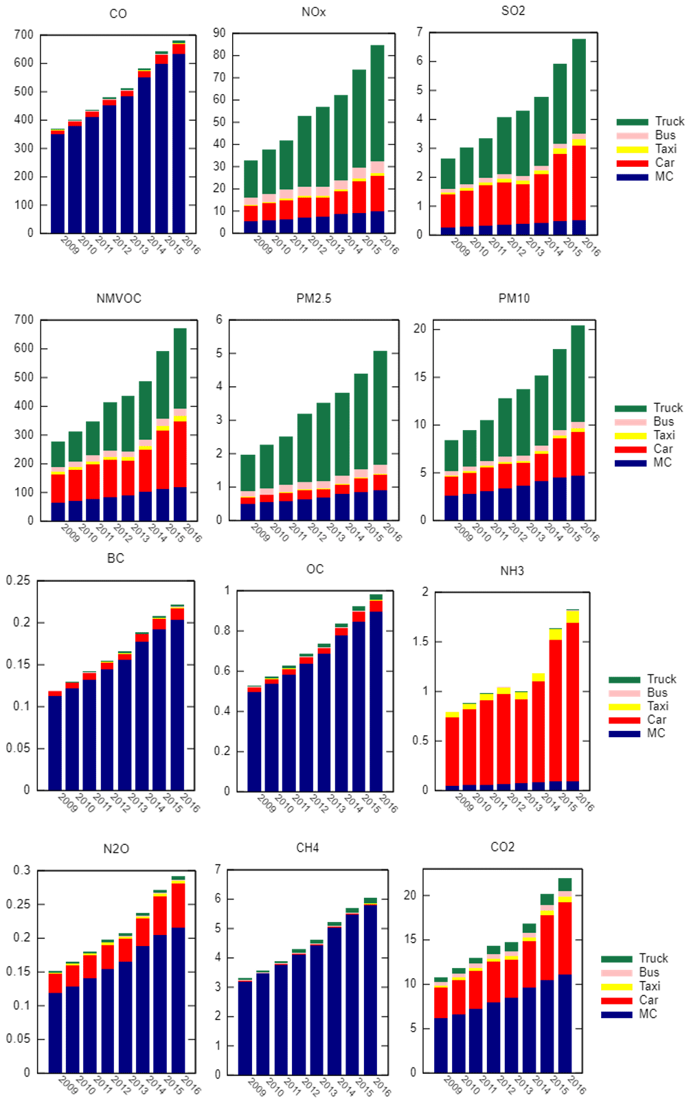
Figure 3Annual emissions of 12 pollutant species in HCMC from 2009 to 2016 for each vehicle type (unit: Gg).
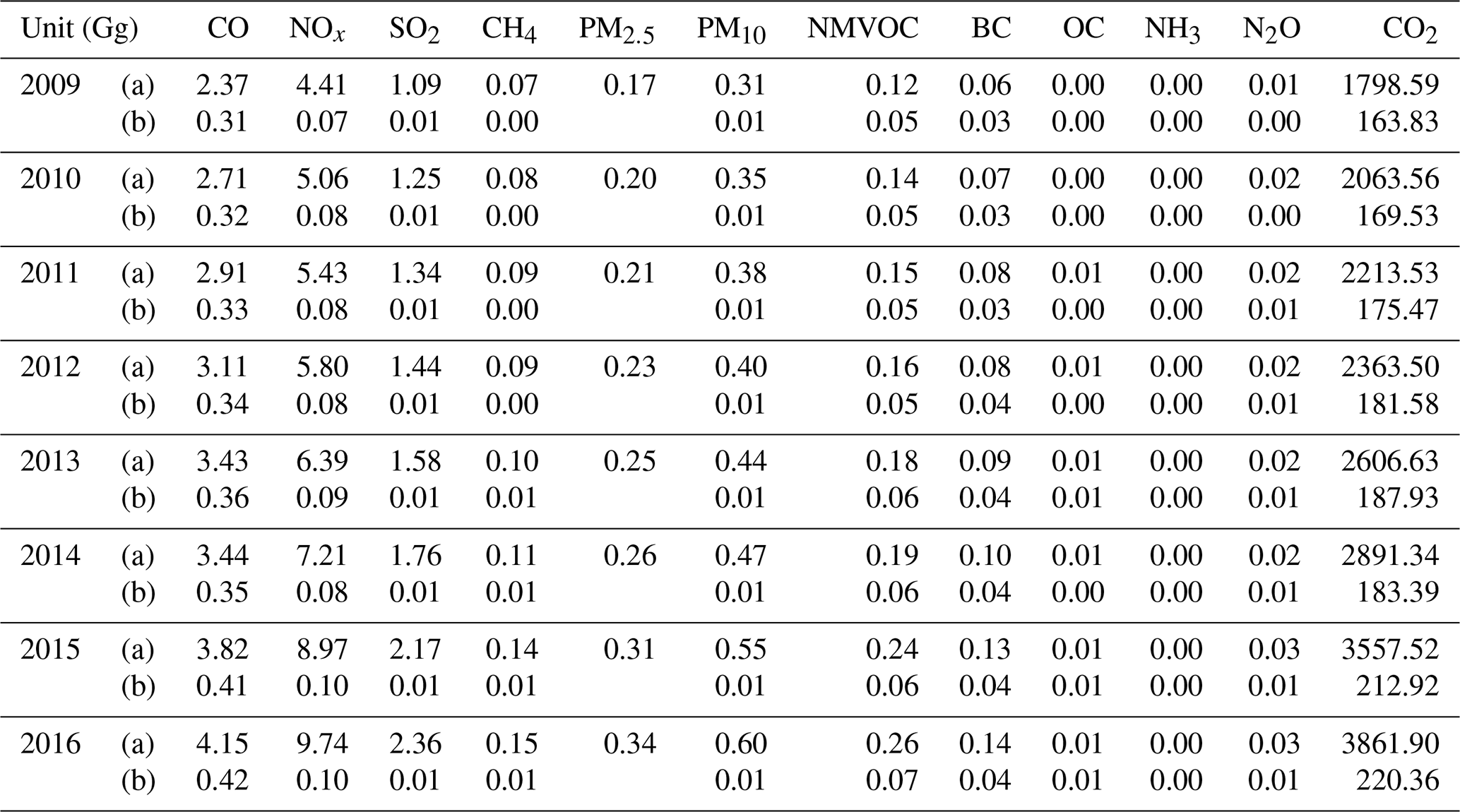
Table 10Annual emissions for each species from the transportation sector in HCMC from 2009 to 2016 (Gg yr−1).
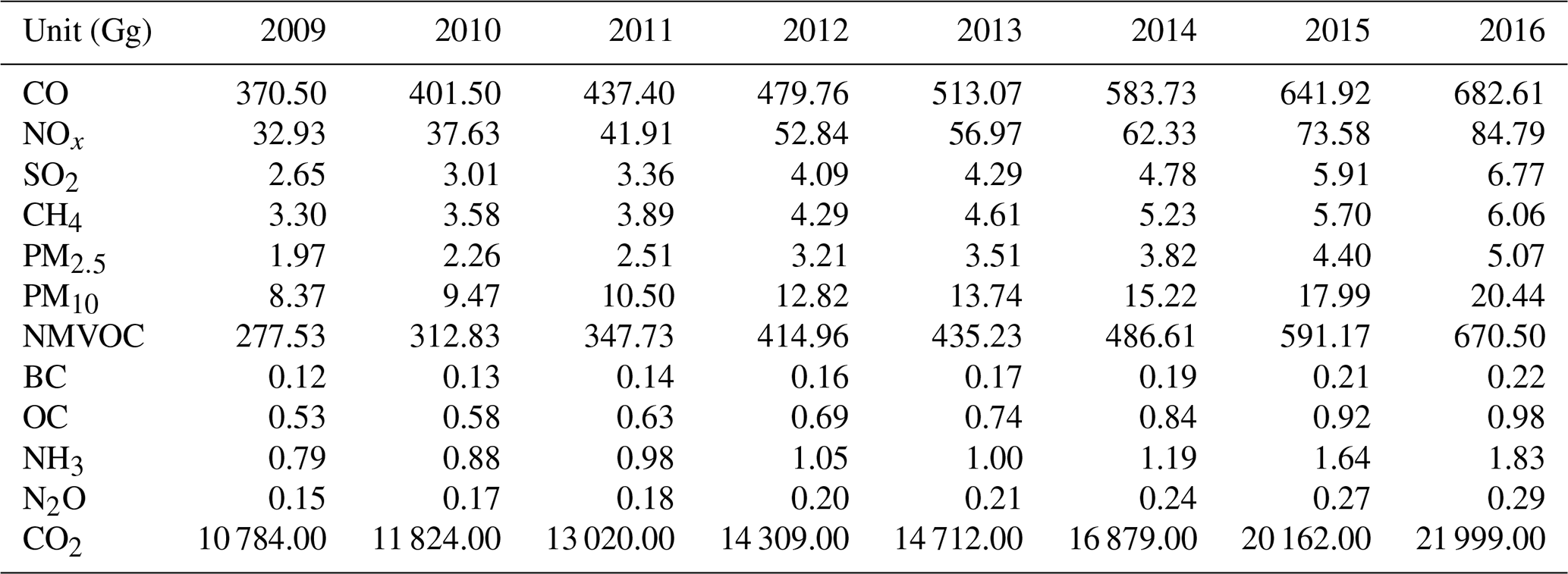
Total CO emissions in 2016 were 682 Gg, increasing by 312 Gg (+98 %) compared to 2009. Over 95 % of CO emission from transportation was accounted for by MCs. In HCMC, the growth rate of MCs reached 180 % over 8 years (from over 4 million to over 7.2 million vehicles). Although the increase rate of personal cars was higher (+130 % from 2009 to 2016), MCs had constantly shared around 90 % of total vehicle population during that period (Fig. 3). Furthermore, the CO emission factor of MCs was by far the highest one among five types of vehicles (12.592 g km−1 per vehicle). This is almost 6 times higher than that of personal cars and taxis.
Over this period, NOx presented a different pattern, despite the same monotonically increasing trend with CO. Total NOx in 2016 was 84.8 Gg (+157.4 %) for HCMC. The majority of NOx emissions were from heavy-duty vehicles (HDVs, trucks; 50 %–61.9 % during the period 2009–2016), followed by personal cars (19 %–21 %). The fact is that HDVs use diesel engines which emit a higher amount of PM and NOx (Reşitoğlu et al., 2015). In addition, the truck fleet in HCMC is quite old (the average age is 11.7 years), leading to a high sharing ratio of outdated engines (75 % of trucks used Euro 2 engines) (Oanh and Van, 2015). As a result, the NOx emission factor of trucks is the highest one among five types of vehicles. Although emission factors of trucks (17 g km−1 per vehicle) and buses (16.954 g km−1 per vehicle) are roughly equal, the dominant population of trucks made it the largest contributor to total NOx emissions from transportation.
Total SO2 emission from on road traffic in 2016 was 6.773 Gg. The emission values more than doubled from 2009 to 2016 (+155.78 %). Again, the contribution was dominated by trucks (39 %–48 %), followed by personal cars (38 %–42 %). Different from CO emissions, MCs were not an important source for SO2. This common vehicle accounts for a modest proportion (7.4 %–10.5 %) compared to others. This trend reflects the highest SO2 emission factor of trucks which use diesel engines (1.06 g km−1 per vehicle).
Total emissions of PM10 and PM2.5 in 2016 from the transportation sector in HCMC were 20.4 and 5.07 Gg (+143 % and 157 %). Showing a similar pattern to NOx, trucks made the highest contributions to emissions of particulate matter (38.4 %–49.5 % and 54.7 %–66.9 % for PM10 and PM2.5, respectively). The reason is that diesel engines emitted much more fine particles than gasoline engines that are mainly found in MCs (Reşitoğlu et al., 2015). EFs of HDVs used in this study are 3.28 and 1.1 g km−1 per vehicle for PM10 and PM2.5, respectively, which are almost 35 and 61 times higher than those of MCs. Consequently, although MCs shared over 90 % of total vehicle population, the dominant emission factors of vehicles using diesel engines made them the main emission sources of PM.
Emission of the aerosols BC and OC showed almost opposite tendencies. Total emissions of BC and OC in 2016 in HCMC were 0.222 and 0.982 Gg (+85 %/+87 %), respectively. MCs made the most considerable contribution to these primary aerosol emissions (92 %–94 %). The remaining transportation types accounted for very small shares (1 %–5 %). This is because we applied emission factors of BC and OC from updated emission factors of air pollutants from vehicle operations in GREET (Greenhouse Gases, Regulated Emissions, and Energy Use in Transportation) using MOVES (MOtor Vehicle Emission Simulator) (Cai et al., 2013). According to this database, MCs are the most common source of BC and OC emissions (0.004 and 0.0178 g km−1 per vehicle).
Regarding greenhouse gases, total emissions of CO2, CH4 and N2O in 2016 in HCMC were 21 999 Gg (+103 %), 6.601 Gg (+100 %) and 0.292 Gg (+92 %), respectively. In the cases of CO2 and N2O, MCs and personal cars are considered the main sources for emissions. A total of 50 %–57 % of CO2 emissions were from MCs, and their proportion decreased by 7 % over 8 years. Personal cars ranked second but their share of the total rose from 32 % to 36.8 % from 2009 to 2016. A similar trend was seen in N2O, although MCs had a larger share for this species than CO2 (74 %–79 %). The contribution of personal cars slowly grew from 18 % to 22 % of total N2O emission from transportation. In terms of CH4, which is important in reducing short-lived climate forcers, the share of MCs was by far the highest (95 %–97 %). The very small share of CH4 emissions in the transportation sector was from other vehicle types. These estimations are in line with other previous studies that claimed diesel engines emit less CO2 and greenhouse gases than similar gasoline ones (Reşitoğlu et al., 2015).
3.1.2 Manufacturing industry and residential building emissions
Table 11 presents annual emissions from fuel consumption in two other key sectors: manufacturing industries and residential buildings. Figure 4 shows the comparison among three key sectors for each species in HCMC from 2009 to 2016. It should be noted that only Scope 1 emissions that occur within the boundary of the city are considered in this sector. Generally speaking, both of these emission sources expressed a much smaller amount of emissions and slower growth paces than transportation.
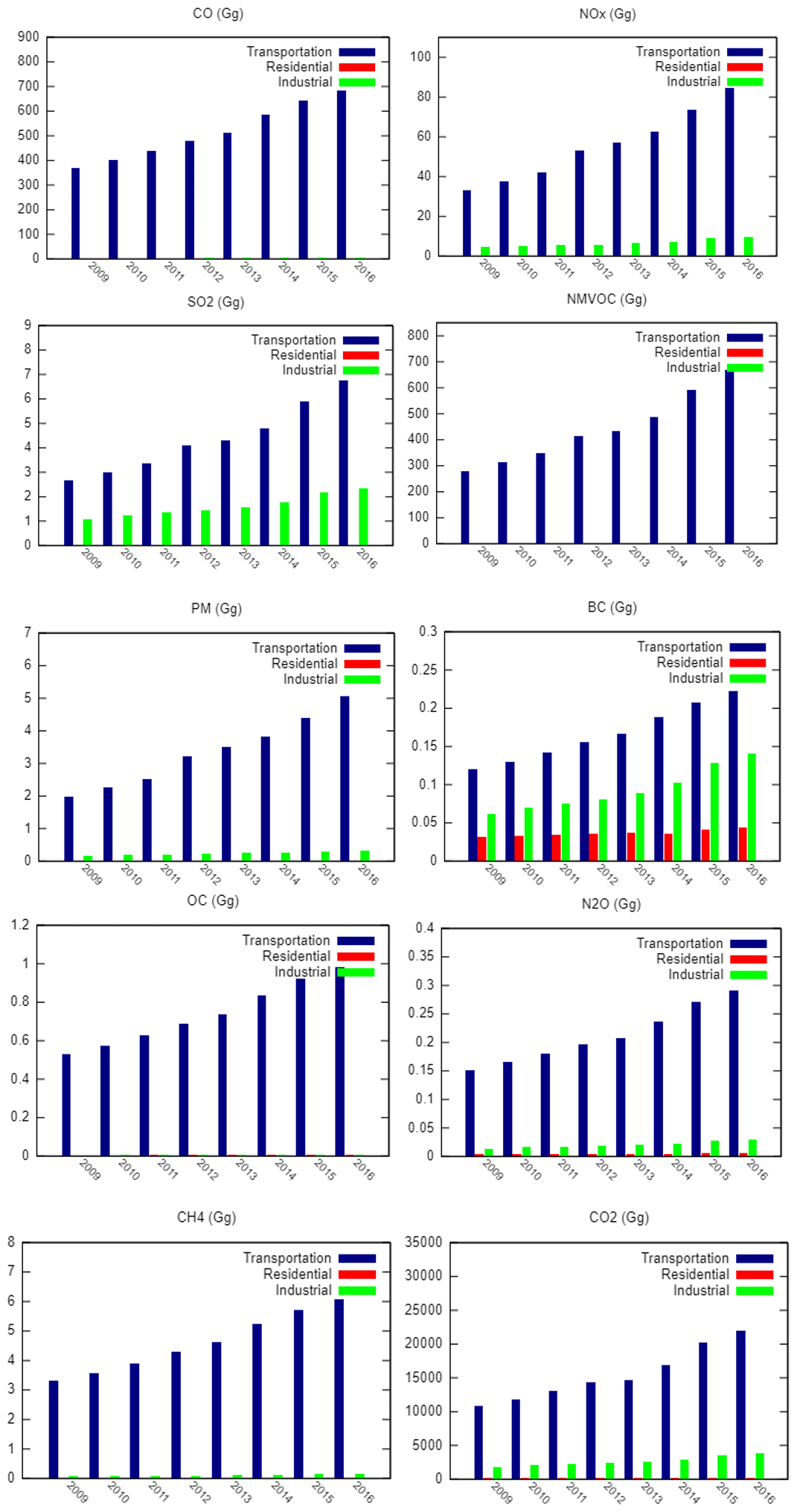
Figure 4Annual emissions of each species in HCMC from 2009 to 2016 for three key sectors (unit: Gg).
Table 11Annual emissions from fuel consumption in manufacturing industries and construction (a) and residential buildings (b) (PM2.5 and PM10 are merged into PM in the residential sector according to ABCEIM by Shrestha et al., 2013).
In terms of manufacturing industries in HCMC, total SO2 emissions from this sector in HCMC increased monotonically from 1.092 to 2.36 Gg (+116 %) over 8 years. However, these amounts are still modest compared to emissions from transport activities, and the gap between the two sectors increased with time. In 2009, emissions of manufacturing industries were less than a half of traffic emissions. About 8 years later, this proportion decreased to 34.8 %. Normally, the main source of sulfur dioxide in the air is industrial activity that processes materials that contain sulfur. However, the explosion of transport activities in HCMC led to the dominant contribution of this sector to SO2 emissions. SO2 is a component of great concern because controlling SO2 emission may have the important co-benefit of reducing the formation of particulate sulfur pollutants, such as fine sulfate particles. NOx emission from manufacturing industries in 2016 was 9.739 Gg, increasing by 120 % over 8 years. Similar to SO2, this accounted for only a very small fraction (almost a ninth) of traffic emissions. This is reasonable because NOx is produced from the reaction of nitrogen and oxygen gases in the air during fuel combustion. In large cities, the highest amount of nitrogen oxide emitted into the atmosphere as air pollution is usually from road transport. This distance is even more profound in the case of CO. In 2016, CO emission from manufacturing industries was 4.152 Gg. Meanwhile, the transportation sector emitted 682.613 Gg, around 160 times higher than manufacturing industries. In addition, emission of CO from manufacturing industries showed a moderate growth rate compared to NOx and SO2, 75 % over 8 years.
Regarding primary particle matter, both PM10 and PM2.5 emissions almost doubled from 2009 to 2016. Total emissions of PM10 and PM2.5 in 2016 were 0.6 and 0.33 Gg (+96 % and 93 %). Again, these amounts of emissions are relatively insignificant compared to emissions from transport activities. However, the sharing ratio among sectors changed for the case of BC. BC emission were still mainly from road transport but the contributions of manufacturing industries to total emissions of this short-lived climate pollutant cannot be neglected. In 2016, the industry sector in HCMC emitted 0.14 Gg (+129 %) BC into the atmosphere, which was equal to 63 % of BC emission from transportation, and this proportion tended to increase. OC emissions differed from BC. The total OC emissions from manufacturing industries in HCMC (2016) were 0.0071 Gg (+86.8 %), which was equal to only 7.2 % of the emissions from transportation activities. Organic carbon has a cooling effect as it reflects light. Meanwhile, black carbon absorbs light. If the ratio of warming particles is higher, sources may have less of a cooling effect. This implies that apart from transportation, reducing short-lived climate forcers cannot disregard the share of manufacturing industries in HCMC.
Total CO2 emission in 2016 from manufacturing industries in HCMC was 3861.89 Gg (+114.7 %). CO2 emissions generally reflect the energy consumption, infrastructure buildup and economic growth. The dominance of energy consumption from traffic activities was confirmed again by the gap in CO2 emission between manufacturing industries and the transportation sector. Emissions of CH4 and N2O from manufacturing industries in 2016 were 0.1512 Gg (+116 %) and 0.03 Gg (+115 %), respectively.
The fuel consumption of the residential sector in big cities mainly includes heating, cooling, lighting, water heating and consumer products. In the GHG emission inventory prepared by JICA, the energy consumed by households in HCMC included only kerosene and liquefied petroleum gas (LPG). Because of tropical climate in HCMC, this energy consumption is generally for cooking/household stoves; the heating and water heating can be excluded. This explains quite trivial shares from the residential sector in total emissions of each pollutant species, although the population explodes in the study area over 8 years (+27.1 %). For example, CO emission from residential buildings in 2016 in HCMC was 0.4189 Gg, which is equivalent to a of manufacturing industry emissions. In addition, our estimation implied that the evolution of household emissions is much slower compared to other sectors. In parallel with 27 % of the population growth in HCMC over 8 years is a 34.5 % increase in greenhouse gases emitted from the residential sector. Meanwhile, CO2 emissions from transportation soared by 104 % during the same period. In fact, the shares in household energy consumption are incommensurate. Particularly in tropical regions, where fuel consumption is mainly used for cooking purposes, the largest contributor is often household electricity consumption, which belongs to Scope 2 emissions. The following section discusses this in more depth.
3.2 Scope 1 and Scope 2 emissions
According to the GHG emission inventory prepared by JICA (2017a), electricity consumption has the highest proportion in terms of manufacturing industry and residential sectors. Therefore, the pattern is quite different from fuel consumption emissions. Scope 2 emissions consider the greenhouse gas CO2 only.
A gradual increasing trend in CO2 emissions from electricity consumption was recorded in both industry and residential sectors (Fig. 5 and Table 12). However, manufacturing industry showed stronger growth (+88 % over 8 years). Consequently, by 2012, CO2 emission from electricity consumption of industry was lower than residential emissions. But from 2013, the emissions of this sector surpassed those from household areas. In 2016, the electricity consumptions from manufacturing industries and residential sectors in HCMC emitted 6985.29 and 6691.43 Gg into the atmosphere, respectively. In addition, the dissimilarity in emissions between fuel consumption and electricity consumption was not the same for industry and household areas. In terms of manufacturing industry, electricity consumption emitted almost double the fuel consumption. Meanwhile, the GHG emissions from electricity consumption of households by far exceeded the fuel consumption of this sector.
Table 12Annual CO2 emissions from electricity consumption in the manufacturing industry and construction sector and residential sector (emission for years marked with * were calculated from electricity consumption provided by JICA (2017a), while other emissions for other years were calculated proportionally with annual gross output of industry at current prices by industry activity and annual population in HCMC).


Figure 5Annual CO2 emissions (unit: Gg) of electricity consumption (EC) and fuel consumption (FC) of manufacturing industry and residential sector in HCMC from 2009 to 2016.
The comparison of CO2 emissions (both Scope 1 and Scope 2) among three key sectors was shown in Fig. 6. Transportation still contributed the highest ratio; its emissions were always double those of manufacturing industry. However, the fastest growth was observed in manufacturing industry (+114.7 %), followed by the transportation sector (+104 %). The lowest emission and the slowest evolution were observed in the residential sector. Emissions from this sector were equivalent to only a third of CO2 emission from traffic in 2016. These findings implied that the mitigation of GHGs in HCMC should consider transportation as the most important source.
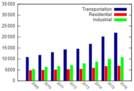
Figure 6Annual CO2 emissions (unit: Gg) of three key sectors: transportation, manufacturing industry and residential in HCMC.
3.3 Spatial distribution
Emission maps can reveal the spatial intensities and where emissions come from. The data are valuable for residences and local authorities in these areas. The data help identify areas of pollution concentration where special activities may be needed to control pollution. Also, they provide necessary input to air quality simulation models.
Figure 7 revealed the spatial distribution of different pollutants as the sum of three key sectors over the study domain in 2016. It should be noted that these 1 km resolution maps show only Scope 1 emissions which are the sum of transportation emissions and emissions from fuel consumption of two other sectors, not including emissions from electricity consumption. According to Fig. 4, transportation emissions are far more dominant than the two other source types, in terms of all pollutant species. It explains the similarity among emission maps of various types of pollution shown in Fig. 7. Relatively high emission densities are found in the central business districts (CBDs) like Quan 1, Quan 4 and Quan 7, because of high road densities in this area. Suburban districts demonstrated a much better situation, like low emission amplitudes observed in Can Gio, Cu Chi and Binh Chanh. Emissions within each kilometer squares in CBDs can be over 1900 times higher than the ones in surrounding districts. According to these maps, abatement strategies of emissions in HCMC should focus on CBDs to improve air quality. If regional EIs like REAS are applied, the 0.25∘ resolution cannot show the spatial distribution within HCMC. Our originality is the use of satellite-derived urban land use morphological maps which allow spatial disaggregation of emissions on the city scale. In a previous study of Ho (2010), the first emission maps were developed for HCMC using road networks as an allocation factor for the transportation sector and population density as an allocation factor for industrial and residential sectors. Our finding about high emission intensities in CBDs is in line with research that stated that the highest emissions were found in the city center, where there is the highest density of streets. Apart from this study, other works only provided the total emissions in HCMC, dismissing the spatial disaggregation. Thus, our approach is advantageous; it enables the mapping of emissions with high reliability in this city in the future.

Figure 7Emission maps of NOx, SO2, CO, PM and CO2 in 2016 in HCMC as the sum of three key sectors: transportation, manufacturing industry and residential.
3.4 Comparison with other inventories
3.4.1 Comparison of transportation emission inventories
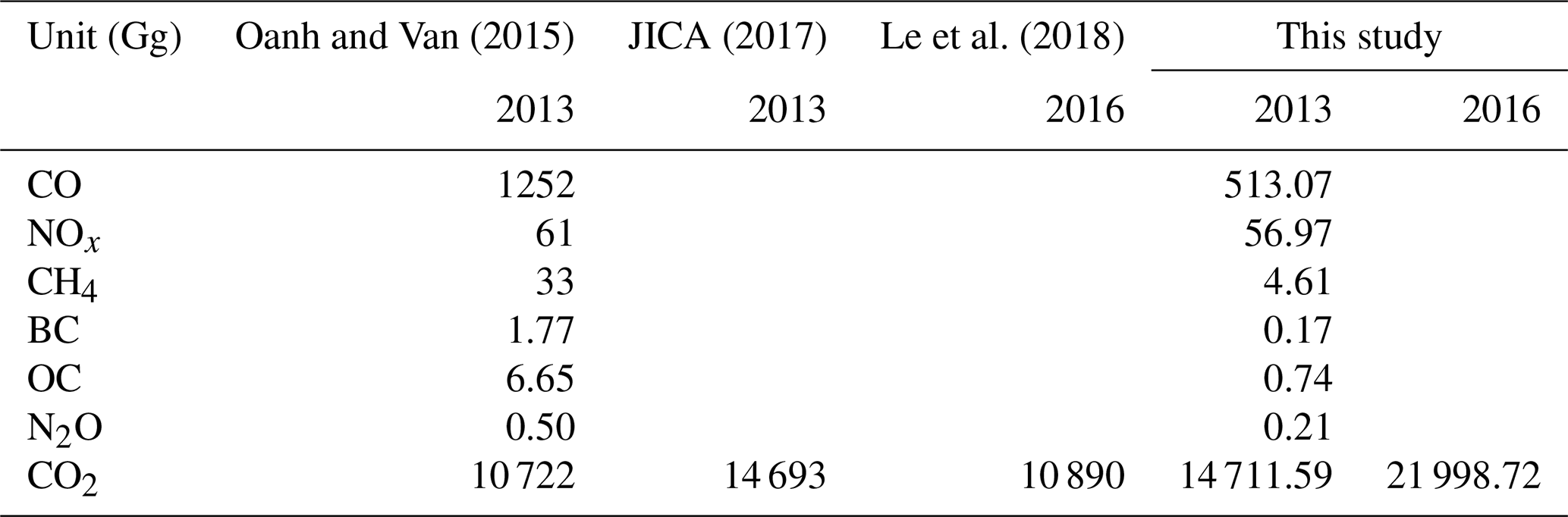
The transportation emissions estimated in this study were compared with four previous studies about vehicle emissions in HCMC (Table 13). The study of Oanh and Van (2015) applied the same equation to estimate emissions of on-road traffic. Activity data included the number of active vehicles, divided by five vehicle types, and daily VKTs of each vehicle type. In addition, this research considered the daily number of startups per vehicle category and average speed to estimate detailed emission factors. EFs were separated into start-up EFs and running EFs. Their output is annual emission in HCMC (2013) for CO, VOCs, NOx, SO2, PM, BC, OC, CO2, N2O and CH4.
Table 13Comparison of transportation emissions estimated in this study with emissions calculated in previous studies for 2013 and 2016. Values in italics refer to emissions estimated for 2013.
The second study is the GHG emission inventory of JICA. This study applied a different method: activity data were fuel consumption of transportation sector (mainly gasoline and diesel), and EFs were extracted from the 2006 IPCC Guidelines.
Another GHG emission inventory for HCMC was the study of Le et al. (2018). This author used activity data that were vehicle counts, by type of vehicle, and daily VKTs were from the study of Oanh and Van (2015). Their vehicle counts were derived from field measurements and vehicle registry data. Regarding the CO2 emission factor, they used country-specific EFs from the COPERT model instead of EFs from the 2006 IPCC guidelines. Noticeably, they divided the vehicle fleet into four types only: MCs, buses, diesel cars and gasoline cars.
Another highly detailed vehicle emission inventory in HCMC was prepared by Ho (2010). The activity data were hourly traffic counts, including five categories, namely cars, light-duty trucks, heavy-duty trucks, buses and MCs. EFs were extracted from literature review and were assumed to be constant in each street category and constant in time. The output is hourly emissions from the vehicle fleet in HCMC. The contribution percentage of each vehicle type for each pollutant in this study was compared with the estimation in this study.
Our CO2 emission in 2013 was quite close to the calculation of JICA, although they applied different approaches to estimate emissions from transportation. But our finding is higher than the estimation of Oanh and Van (2015), around 4000 Gg. We applied the same numbers of active vehicles and daily VKTs used in the research of Oanh and Van (2015), but they used EFs in much more detail. As a result, the different emission factors are likely the reason for this gap. In comparison with the findings of Le et al. (2018), our CO2 emissions in 2016 are double. As mentioned before, this author classified vehicle fleet in HCMC into only four types, without considering trucks. In addition, the difference in daily VKTs, vehicle population and emission factor is likely to contribute to the inconsistency with our calculation.
In terms of other pollutants, estimations were lower by factors of 2–10 in comparison with the study of Oanh and Van (2015). The vehicle populations and daily VKTs were the same for both studies. The smallest gap was observed for NOx emissions, while BC and OC emissions showed significant distinctions. The EF dataset used in the study of Oanh and Van (2015) was not clarified in their publication, but it is expected to explain the gap between the two studies. Their study applied the International Vehicle Emissions (IVE) model to produce the EFs that are relevant to the local driving conditions and local fleet composition, and it considers the engine technology distribution in the vehicle fleet. Meanwhile, this study applied constant emission factors from different previous research about transportation emissions in HCMC, Hanoi and China.
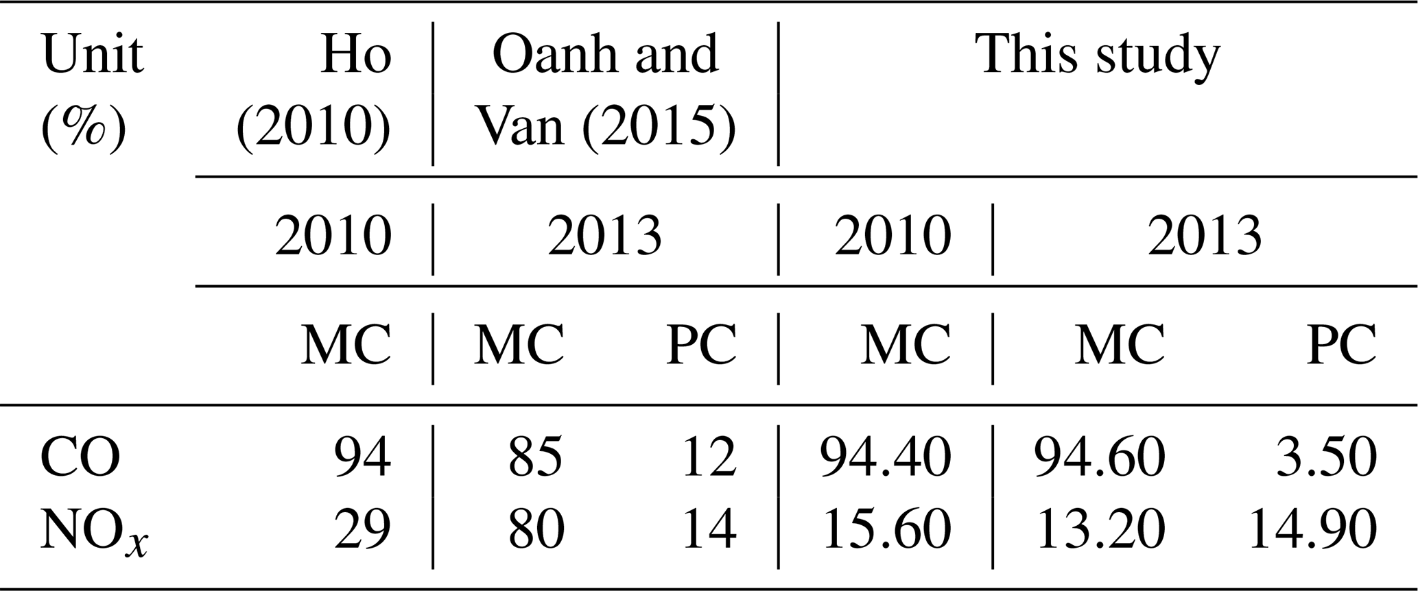
Regarding the sharing ratio of emissions from MCs and personal cars (PCs) in this study and previous studies for 2010 and 2013, our results are relatively consistent with the research of Ho (2010) (Table 14). MCs are responsible for over 94 % of CO emission from on-road traffic, 29 % and 15.6 % of NOx emissions in the study of Ho (2010) and in this study, respectively. In comparison with the study of Oanh and Van (2015), the sharing proportion of MC from my estimation is higher, but the contribution from personal cars is lower in terms of CO. A significant gap was recorded in the sharing percentage of MCs for NOx emission. According to their calculation, the MC fleet accounts for 80 % of total NOx emission from transportation in HCMC. This ratio was much higher than the findings of Ho (2010) (29 %) for vehicle emissions in 2010. As mentioned before, this study applied the same number of active vehicles and the same daily VKT data as the study of Oanh and Van (2015) for emissions in 2013. As a result, this gap is expected to come from inconsistent EF datasets between two studies.
Table 14Comparison of sharing ratios of emissions from MCs and personal cars (PCs) in this study and previous studies for 2010 and 2013 (unit: %).
3.4.2 Comparison with the REAS v2.1 inventory
The general information of REASv2.1 and the data sources applied for three sectors, transportation, manufacturing industry and residential, are mentioned in the Supplement (Tables S1 and S2). REAS2.1 mainly used the national statistical data for their activity data. Then the spatial allocation was based on road network or population data to create grid maps with 0.25∘ resolution. Table 15 shows the comparison between the estimations in this study for 2009 and the estimation of REAS 2.1 for three key sectors in Kurokawa et al. (2013). The transportation emissions from REAS for 2008 were much lower than our calculation for 2009, except BC, by factors of 1.5 to 10, depending on pollutant species. It is worth noticing that the data sources applied in two studies were not the same. REAS was based on vehicle numbers, annual distance traveled and emission factors to estimate vehicle emissions. Their vehicle population was the national one, and then total emissions were allocated to HCMC using the road network. Thus it is likely that the calculation underestimated the emissions from a traffic hotspot such as HCMC. In addition, the gap between their annual VKTs and our daily VKTs could be a cause.
Table 15Comparison of transportation, industry and domestic emissions estimated for 2009 in this study and emissions estimated by REAS 2.1 for 2008. Italic numbers refer to emissions provided by REAS 2.1.
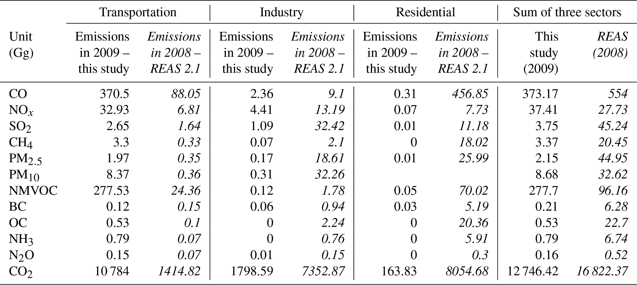
Conversely, the estimation of industry and residential emissions of REASv2.1 surpassed the findings in this study by factors of 3–104. The difference for the residential sector is more significant than for industry. In this comparison, only Scope 1 emissions of HCMC were compared with REAS emissions. So both studies applied fuel consumption as activity data. But REAS fuel consumption data were national data provided by the International Energy Agency (IEA) energy balance database, and the data applied in this study are annual sale data provided by the HCMC Department of Industry and Trade (DOIT) and fuel companies. Apart from different sources of activity data, Table 16 compares the EFs of fuel consumption in these two sectors that were applied in two studies. In addition, for countries which do not have their own emission inventories, REAS adopted emission factors from 1980 to 2003 from many sources, including Asian emission inventories. Meanwhile, this study applied EFs provided by ABCEIM from Shrestha et al. (2013). REAS 2.1 applied EFs of oil and gas only. In terms of the industry sector, EFs of NOx and NMVOC were pretty similar. But EFs of CO and SO2 from REAS are much higher. The CO emission factor was over double that applied in this study. Regarding oil, the SO2 emission factor was over 10 times higher than our EF. This trivial consistency was seen in EFs used in the residential sector as well (Table 17).
Table 16Comparison of emission factors used for the industry sector in this study and in REAS v2.1. Italic numbers refer to emission factors used in REAS 2.1.
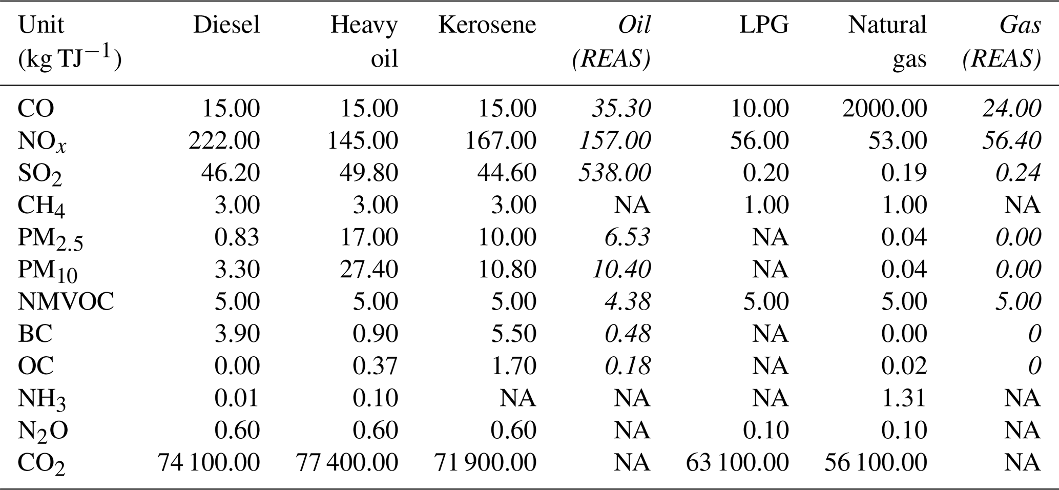
NA – not available.
Table 17Comparison of emission factors used for the domestic sector in this study and in REAS v2.1. Italic numbers refer to emission factors used in REAS 2.1.
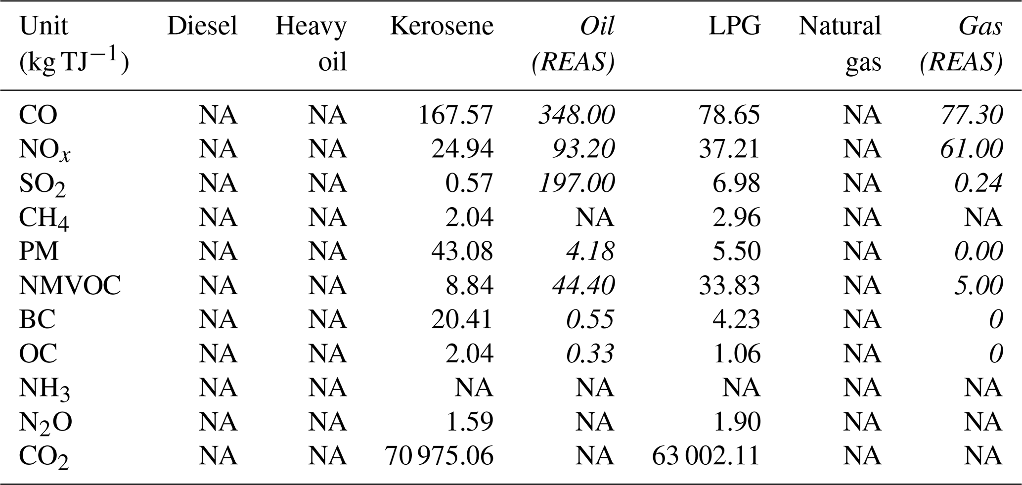
NA – not available.
The large discrepancies can be seen in the sum of emissions from fuel consumption of three key sectors. The gap of under 25 % between our EI and REASv2.1 was recorded only in the cases of CO, NOx and CO2. According to the big gaps drawn from this analysis, the limitation when comparing a regional emission inventory with a local emission inventory can be implied. This inconsistency is expected due to the differences in activity data and EF databases. Again, the limitations of downscaling a regional EI to the community scale can be seen here. The regional scale is likely to underestimate the most profound emission sector like transportation and show the overestimation of other sectors when applying population as the only spatial allocation index.
3.5 Uncertainty
In this study, in order to calculate the uncertainties of the estimated EI, the error range of each of the inputs including activity data and emission factors is determined, computed or collected from different sources. The Monte Carlo simulation is a common method for analyzing uncertainty propagation in air quality studies (Ho, 2010). To calculate the uncertainty ranges of emissions of three key sectors in HCMC, the Monte Carlo method is applied to select random values of EFs, activity data and other estimation parameters from within their individual probability density functions (PDF) and to calculate the corresponding emission values. This process is repeated many times, and the results of each simulation contribute to an overall emission PDF. In fact, it is fundamentally hard to quantify the uncertainties of parameters, and for most inputs assessment of the PDF is subjective. Accordingly, in previous studies and good practice guidance and uncertainty management in national greenhouse gas inventories by the IPCC, 2006, coefficients of variation for both activity data and EFs were determined based on expert judgment. When running a Monte Carlo simulation, the activity data and EFs in this study are assumed to be independent. Regarding the transportation sector, assuming a normal distribution, the relative uncertainties for vehicle population and daily VKTs are 5 % and 10 %, respectively. For activity data of stationary sources, we relied on fuel consumptions from 2013 to 2015 collected from the HCMC Department of Industry and Trade (JICA, 2015): annual gross output of manufacturing industry and annual population in HCMC provided by HCMC statistical yearbook. So these activity data were assumed to be normally distributed with an error range of 2 %. EFs of transportation and fuel consumption of two other sectors are mainly based on detailed experiments, so lognormal distribution might be a reasonable assumption. Their uncertainties are adopted from previous research and good practice guidance and uncertainty management in national greenhouse gas inventories by the IPCC (2006).
Table 18Uncertainties (%) of emissions of three key sectors in HCMC.
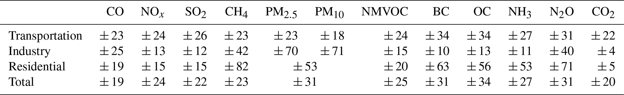
Table 18 presents the estimated uncertainties of emissions by sector in HCMC (2016). Uncertainties of total emissions from three key sectors are as follows: ±19 % for CO, ±24 % for NOx, ±22 % for SO2, ±23 % for CH4, ±31 % for PM, ±25 % for NMVOCs, ±31 % for BC, ±34 % for OC, ±27 % for NH3, ±31 % for N2O and ±20 % for CO2. In general, error ranges of CO2, CO and SO2 are the smallest. Meanwhile, those of PM, BC and OC are relatively large. The reason for a relatively high accuracy of SO2 and CO2 emissions is that their main emission sources are complete combustion. Whereas those of PM species have larger uncertainties because they are emitted from burning at low temperatures. In addition, the sensitivity analysis of Monte Carlo shows that the accuracy of transportation emissions is mainly impacted by the annual number of motorcycles and the number of trucks. The uncertainty of heavy oil consumption is the largest driver causing the error range of resulting emissions from the manufacturing industry sector. Meanwhile, the accuracy of residential emissions is mostly decided by kerosene consumption. The activity data in this study were obtained directly from statistics, so their accuracy is higher than those applied in regional EIs such as REAS. As a result, the uncertainties of local emissions from all three sectors are smaller than the ones provided by REAS.
We developed a consistent and continuous EI for three key sectors at a local scale. Our objective is to fill the gap among inherent EIs developed for HCMC previously. The activity data and EFs were synthesized from various sources. This local emission inventory includes most major air pollutants and greenhouse gases: SO2, NOx, CO, NMVOC, PM10, PM2.5, BC, OC, NH3, CH4, N2O and CO2. The target years are from 2009 to 2016. Emissions are estimated for area within the boundary of HCMC and are allocated to grids at a 1 km resolution.
In terms of transportation, our results implied that the contribution of this sector to total emission in HCMC is the largest. Vehicle fleet in HCMC emitted over 682 Gg CO, 84.8 Gg NOx, 20.4 Gg PM10 and 22 000 Gg CO2 in 2016. The overall emission of this sector increased significantly from 2009 to 2016, mainly because of the explosion of the vehicle population. The emissions of CO, NOx, SO2 and CO2 from traffic in 2016 in HCMC were 80 %, 160 %, 150 % and 103 % more than those in 2009, respectively. Among five vehicle types, MCs contributed around 94 % to total CO emission, 14 % to total NOx emission and 50 %–60 % to CO2 emission. Regarding NOx, SO2 and PM, trucks are the biggest emission source, and the sharing of personal cars was considerable in terms of NMVOCs and CO2.
The emissions of the manufacturing industry and residential sectors include both fuel consumption and electricity consumption. Electricity consumption is the most profound contributor. In 2016, the electricity consumption of the manufacturing industry and residential sectors in HCMC emitted 6985 and 6691 Gg of CO2, respectively, increasing by 87 % and 45 % in comparison with 2009, respectively. Considering fuel consumption only, both these sectors account for a very small percentage in comparison with transportation, and the growing trend is slower compared to vehicle emission as well. The sum of CO2 emission from fuel consumption and electricity consumption of these two stationary energy sectors still could not exceed the transportation sector. In 2016, the vehicle fleet emitted 22 000 Gg CO2, almost double that of the manufacturing sector. Meanwhile, residential area contributed 7000 Gg CO2 only. According to Monte Carlo analysis, uncertainties of total emissions from three key sectors are as follows: ±19 % for CO, ±24 % for NOx, ±22 % for SO2, ±23 % for CH4, ±31 % for PM, ±25 % for NMVOC, ±31 % for BC, ±34 % for OC, ±27 % for NH3, ±31 % for N2O and ±20 % for CO2.
Regarding spatial allocation of three key emission sectors, the CBDs like Quan 1, Quan 4 and Quan 7 express the highest emission intensities, which can be over 1900 times the ones in outlying areas. Thus, the policy makers must consider suitable future activities and regulations to control pollution in HCMC focusing on central regions. The estimations of this study showed the relative agreement with several local inherent EIs, in terms of total amount of emissions and sharing ratio among elements of EI. However, the big gap was observed when comparing with REASv2.1. The different data sources of activity data and the EF database explained this difference. Again, this implied the inevitable gap between regional and local EIs. This situation caused challenges in compiling consistent, continuous yet comparable data with processor EIs like REAS.
Our study applied the activity data and EFs synthesized from various sources, and a number of limitations and uncertainties were noted. Regarding the transportation sector, this study assumed constant VKTs, EFs of the vehicle fleet and road network over 8 years. The technology standard distribution for each vehicle type which impacts the change in EFs was neglected as well. Apart from MCs and personal cars, the populations of buses, taxis and trucks remain uncertain due to the limitation of statistical data. Because traffic shares the highest ratio of emissions among three primary sectors, if any of these factors, VKTs, EFs and road network, are improved, the accuracy of total emissions in HCMC can be enhanced considerably.
In terms of manufacturing and residential sectors, the activity data come from fuel consumption and electricity consumption data provided by the HCMC Department of Industry and Trade (DOIT) and EVN, respectively. Meanwhile, this study considers emissions within the boundary of HCMC only. The uncertainty relating to the administrative boundary of sale data provided by DOIT and EVN can impact the accuracy of our estimations. Because industrial zones are often located around the ring road and around the city boundary, including or excluding these emission zones could lead to considerable change in total emission amount. Apart from that, the grid EFs on electricity consumption were only available in three years, 2013, 2014 and 2015. Electricity consumption is typically the largest emission source regarding stationary energy emission. Thus the limitation of these EFs could have a big impact on final GHG emission amount of HCMC. Moreover, EFs of fuel consumption and removal efficiencies for both stationary energy sectors were assumed to be constant over 8 years, meaning the technology evolution was not considered.
With updated methods and substantial new data on local emission sources, a city-scale emission inventory of 12 air pollutants has been developed for HCMC, Vietnam, for 8 years, 2009–2016. Through statistical data, EFs adopted from previous studies in Asia and spatial emission distributions, the total emissions for three major sources (transportation, manufacturing industries and residential buildings) are estimated and mapped. Emissions in the city are dominated by traffic activities, followed by manufacturing industries and household areas. All these sectors show the increases in emissions, although the growth rates are not the same.
In the future, to improve this local emission inventory, it is necessary to include other sectors such as waste, industrial processing and product use (IPPU) and agriculture, forestry and other land use (AFOLU) for a comprehensive EI. In addition, since HCMC is located in a tropical region, the significant monthly variations in fuel consumption and electricity consumption of stationary energy sectors were not expected. Improving the level of detail of EIs from annual to monthly is still required. The next step is using the EI as input data of atmospheric chemistry models and conducting the comparison to independently derived data. In this case, remote sensing data and observed data provided by air quality monitoring networks can be the answer. In addition, with available local EIs, policy makers can see the quantitative improvement of air quality by atmospheric chemistry models using adjusted emission inventories according to mitigation solutions as input data. In addition, the improvement of local activity data and emission factors could enhance the reliability of this EI.
The continuous growth in emissions from all three sectors implies that substantial efforts should be undertaken to achieve targets in emission reduction in HCMC. According to our calculations, emission abatement should prioritize transportation activities. To decrease the total emissions of this dominant sector, a number of air pollution control solutions are proposed: exhaust control policies for MCs and trucks to improve their emission factors and replacing personal vehicles with public transport. It is a fact that the majority of MCs and trucks in HCMC use old standard engines as mentioned above, so the use of modern engines will lead to significant improvements in air quality in this city. In addition, because emissions from fuel consumption only account for small proportions, the reduction in grid emission factors of electricity consumption could have a remarkable impact on emissions from manufacturing industry and residential building sectors. This can be achieved by the transition from coal-fired power to other forms of clean energy like hydroelectricity or solar power. According to our emission maps, the pollution control solutions should focus on central business districts where the traffic intensities are high. This area also has the highest population density. Thus, the emission mitigation for CBDs will benefit not only the GHG reduction, but also the improvement of human exposure to air pollution.
Our originality is the use of satellite-derived urban land use morphological maps for spatial distribution of area emission sources. Conventionally, the existing regional inventories based on surrogate statistics such as fuel consumption, employment and population as spatial proxies of grid allocation. This can introduce a large uncertainty when downscaling to community-scale EI because its assumption is based on the linear relationship between the proxy value and the emissions. In addition, these statistics are often adopted from fieldwork-based inventories. Although fieldwork-based data can be highly accurate, they are labor-intensive and cannot be performed frequently. The use of those existing spatial distribution surrogates also neglects the effects of urban sprawl that is evident in big cities. It is desirable to have access to revised spatial allocation factors that may be more representative of spatial distributions at the community scale and more available. And even if statistical data are inaccessible in other cities, remote sensing data can be used. Remote sensing data can be updated frequently. Thus, the use of satellite images makes spatial disaggregation updates quite simple and efficient. In addition, they are the best tool to represent urban expansion and land use change, so they ensure the accuracy of grid allocation when a closely related spatial activity surrogate is needed to compile EIs on a local scale.
Gridded emission datasets at 1 km resolution for three key sectors from 2009 to 2016 are available from the corresponding author upon request.
The supplement related to this article is available online at: https://doi.org/10.5194/acp-21-2795-2021-supplement.
TTQN and WT conducted the study design. TTQN contributed to actual works for development of the emission inventory such as collecting data and information, setting parameters, calculating emissions, and creating final datasets. PM conducted urban morphology mapping. TTQN prepared the manuscript with contributions from WT and PM. SH edited and completed the manuscript.
The authors declare that they have no conflict of interest.
This research is financially supported by the Research Institute for Humanity and Nature (RIHN: a constituent member of NIHU) project no. 14200133 (Aakash).
This research has been supported by the Research Institute for Humanity and Nature (project grant no. 14200133).
This paper was edited by Alex B. Guenther and reviewed by Beatriz Aristizabal and Yuan Ren.
Ahlvik, P., Eggleston, S., Gorissen, N., Hassel, D., Hickman, A.-J., Joumard, R., Ntziachristos, L., Rijkeboer, R., Samaras, Z., and Zierock, K.-H.: COPERTII Methodology and Emission Factors, Draft Final Report, European Environment Agency, European Topic Center on Air Emissions, ©EEA, Copenhagen, 1998.
Belalcazar, L. C.: Alternative techniques to assess road traffic emissions, PhD Thesis, National University of Colombia, Bogotá, Colombia, 2009.
Cai, H., Burnham, A., and Wang, M.: Updated Emission Factors of Air Pollutants from Vehicle Operations in GREETTM Using MOVES, Technical Report, Energy Assessment Section, Energy Systems Division, Argonne National Laboratory, USA, available at: https://greet.es.anl.gov/files/vehicles-13 (last access: 18 February 2021), 2013.
Creutzig, F., McGlynn, E., Minx, J., and Edenhofer, O.: Climate policies for road transport revisited (I): Evaluation of the current framework, Energ. Policy, 39, 2396–2406, 2011.
EEA Report: EMEP/EEA air pollutant emission inventory guidebook 2009, Technical guidance to prepare national emission inventories, ©EEA, Copenhagen, https://doi.org/10.2800/23924, 2009.
Gómez, C. D., González, C. M., Osses, M., and Aristizábal, B. H.: Spatial and temporal disaggregation of the on-road vehicle emission inventory in a medium-sized Andean city. Comparison of GIS-based top-down methodologies, Atmos. Environ., 179, 142–155, https://doi.org/10.1016/j.atmosenv.2018.01.049, 2018.
GreenID: Center Green Innovation, Air pollution report, Technical report, Green Innovation Center, Vietnam, 2018.
HCMC Statistical Office: HCMC Statistical Yearbook 2013, General Statistics Office, Vietnam, 2013.
HCMC Statistical Office: HCMC Statistical Yearbook 2014, General Statistics Office, Vietnam, 2014.
HCMC Statistical Office: HCMC Statistical Yearbook 2015, General Statistics Office, Vietnam, 2015.
HCMC Statistical Office: HCMC Statistical Yearbook 2016, General Statistics Office, Vietnam, 2016.
He, L. Q., Song, J. H., Hu, J. N., Xie, S. X., and Zu, L.: An investigation of the CH4 and N2O emission factors of light-duty gasoline vehicles, Huan Jing Ke Xue, 35, 4489–4494, 2014 (in Chinese).
Ho, B. Q.: Optimal Methodology to Generate Road Traffic Emissions for Air Quality Modeling: Application to Ho Chi Minh City, PhD thesis, Ecole Polytechnique Fédérale de Lausanne, Switzerland, 2010.
Ho, B. Q., Clappier, A., Zarate, E., and van den Bergh, H.: Air quality meso scale modelling in Ho Chi Minh city evaluation of some strategies efficiency to reduce pollution, Vietnam Science snd Technology Development, 9, 5, 2006.
Ho, B. Q., Vu, H. N. K., Nguyen, T. T., and Nguyen, T. T. H.: A combination of bottom-up and top-down approaches for calculating of air emission for developing countries: a case of Ho Chi Minh City, Vietnam, Air Qual. Atmos. Hlth., 12, 1059–1072, https://doi.org/10.1007/s11869-019-00722-8, 2019.
Hung, N. T.: Traffic Emission Inventory for Hanoi, Vietnam, International Workshop on Air Quality in Asia Inventory, 24 June 2014, Hanoi, Vietnam, 2014.
IPCC: Revised 1996 IPCC Guidelines for National Greenhouse Gas Inventories, prepared by the National Greenhouse Gas Inventories Programme, edited by: Houghton, J. T., Meira Filho, L. G., Lim, B., Treanton, K., Mamaty, I., Bonduki, Y., Griggs, D. J., and Callender, B. A., UK Meteorological Office, UK, 1996.
IPCC: 2006 IPCC Guidelines for National Greenhouse Gas Inventories, in: Climate Change 2014: Mitigation of Climate Change, Contribution of Working Group III to the Fifth Assessment Report of the Intergovernmental Panel on Climate Change, edited by: Eggelston, S., Buendia, L., Miwa, K., Ngara, T., and Tanabe, K., Institute for Global Environmental Strategies (IGES), IPCC, Japan, 1–33, https://doi.org/10.1017/CBO9781107415324, 2006.
Jacob, D. J., Crawford, J. H., Kleb, M. M., Connors, V. S., Bendura, R. J., Raper, J. L., Sachse, G. W., Gille, J. C., Emmons, L., and Heald, C. L.: Transport and Chemical Evolution over the Pacific (TRACE-P) Aircraft Mission: Design, Execution, and First Results, J. Geophys. Res., 108, 9000, https://doi.org/10.1029/2002jd003276, 2003.
JICA: The Study on the Urban Transport Master Plan and Feasibility Study in City Metropolitan Area, Hochiminh city, Vietnam, HOUSTRANS Project Report, JICA, Japan, 2004.
JICA: Data collection survey on traffic conditions of southern roads and bridges, Vietnam, Final report, JICA, Japan, 2016.
JICA: GHG inventory of Ho Chi Minh city, Project report, JICA, Japan, 2017a.
JICA: City-Level GHG Inventory Preparation Manual, Project to Support the Planning and Implementation of NAMAs in a MRV Manner, JICA, Japan, 2017b.
Kato, N. and Akimoto, H.: Anthropogenic emissions of SO2 and NOx in Asia: Emission inventories, Atmos. Environ. A-Gen., 26, 2997–3017, 1992.
Kühlwein, J., Wickert, B., Trukenmüller, A., Theloke, J., and Friedrich, R.: Emission modelling in high spatial and temporal resolution and calculation of pollutant concentrations for comparisons with measured concentrations, Atmos. Environ., 36, 7–18, https://doi.org/10.1016/S1352-2310(02)00209-1, 2002.
Kurokawa, J. and Ohara, T.: Long-term historical trends in air pollutant emissions in Asia: Regional Emission inventory in ASia (REAS) version 3, Atmos. Chem. Phys., 20, 12761–12793, https://doi.org/10.5194/acp-20-12761-2020, 2020.
Kurokawa, J., Ohara, T., Morikawa, T., Hanayama, S., Janssens-Maenhout, G., Fukui, T., Kawashima, K., and Akimoto, H.: Emissions of air pollutants and greenhouse gases over Asian regions during 2000–2008: Regional Emission inventory in ASia (REAS) version 2, Atmos. Chem. Phys., 13, 11019–11058, https://doi.org/10.5194/acp-13-11019-2013, 2013.
Le, L. T. P. and Leung, A.: Carbon Emissions Assessment of Urban Transport – A New Approach for 10 Major Vietnamese cities, Cities and Climate Change Science Conference, Edmonton, Canada, 5–7 March 2018, https://doi.org/10.13140/RG.2.2.21726.33606, 2018.
Li, M., Zhang, Q., Kurokawa, J.-I., Woo, J.-H., He, K., Lu, Z., Ohara, T., Song, Y., Streets, D. G., Carmichael, G. R., Cheng, Y., Hong, C., Huo, H., Jiang, X., Kang, S., Liu, F., Su, H., and Zheng, B.: MIX: a mosaic Asian anthropogenic emission inventory under the international collaboration framework of the MICS-Asia and HTAP, Atmos. Chem. Phys., 17, 935–963, https://doi.org/10.5194/acp-17-935-2017, 2017.
López-Aparicio, S., Guevara, M., Thunis, P., Cuvelier, K., and Tarrasón, L.: Assessment of discrepancies between bottom-up and regional emission inventories in Norwegian urban areas, Atmos. Environ., 154, 285–296, https://doi.org/10.1016/j.atmosenv.2017.02.004, 2017.
Misra, P.: Analyzing impact of socio-economic development and land-use change on urban air quality in India, PhD thesis, University of Tokyo, Tokyo, Japan, 2018.
Misra, P., Imasu, R., and Takeuchi, W.: Impact of Urban Growth on Air Quality in Indian Cities Using Hierarchical Bayesian Approach, Atmosphere, 10, 517, https://doi.org/10.3390/atmos10090517, 2019.
Oanh, N. T. K and Van, H. H.: Comparative assessment of traffic fleets in Asian cities for emission inventory and analysis of co-benefit from faster vehicle technology intrusion, International Emission Inventory Conference, 12–16 April 2015, San Diego, USA, https://doi.org/10.13140/RG.2.1.4691.3040, 2015.
Oanh, N. T. K., Phuong, M. T. T., and Permadi, D. A.: Analysis of motorcycle fleet in Hanoi for estimation of air pollution emission and climate mitigation co-benefit of technology implementation, Atmos. Environ., 59, 438–448, 2012.
Ohara, T., Akimoto, H., Kurokawa, J., Horii, N., Yamaji, K., Yan, X., and Hayasaka, T.: An Asian emission inventory of anthropogenic emission sources for the period 1980–2020, Atmos. Chem. Phys., 7, 4419–4444, https://doi.org/10.5194/acp-7-4419-2007, 2007.
Reşitoğlu, İ. A., Altinişik, K., and Keskin, A.: The pollutant emissions from diesel-engine vehicles and exhaust aftertreatment systems, Clean Techn. Environ. Policy, 17, 15–27, https://doi.org/10.1007/s10098-014-0793-9, 2015.
Saide, P., Zah, R., Osses, M., Ossés de Eicker, M.: Spatial disaggregation of traffic emission inventories in large cities using simplified top-down methods, Atmos. Environ., 43, 4914–4923, https://doi.org/10.1016/j.atmosenv.2009.07.013, 2009.
Shrestha, R. M., Kim Oanh, N. T., Shrestha, R. P., Rupakheti, M., Rajeshwari, S., Permadi, D. A., Kanabkaew, T., and Iyngararasan, M.: Atmospheric Brown Clouds (ABC) Emission Inventory Manual, United Nations Environment Programme, Nairobi, Kenya, 2013.
Tadono, T., Takaku, J., Tsutsui, K., Oda, F., and Nagai, H.: Status of “ALOS World 3D (AW3D)” global DSM generation, in: Proceedings of the IEEE International Geoscience and Remote Sensing Symposium (IGARSS), 26–31 July 2015, Milan, Italy, 3822–3825, https://doi.org/10.1109/IGARSS.2015.7326657, 2015.
Trang, T. T., Van, H. H., and Oanh, N. T. K.: Traffic emission inventory for estimation of air quality and climate co-benefits of faster vehicle technology intrusion in Hanoi, Vietnam, Carbon Manag., 6, 117–128, https://doi.org/10.1080/17583004.2015.1093694, 2015.
Trombetti, M., Thunis, P., Bessagnet, B., Clappier, A., Couvidat, F., Guevara, M., Kuenen, J., and López-Aparicio, S.: Spatial inter-comparison of Top-down emission inventories in European urban areas, Atmos. Environ., 173, 142–156, https://doi.org/10.1016/j.atmosenv.2017.10.032, 2018.
Yale Center for Environmental Law and Policy: Global metrics for the environment: Ranking country performance on high-priority environmental issues, Yale University, New Haven, USA, 2018.
Zhang, Q., Streets, D. G., Carmichael, G. R., He, K. B., Huo, H., Kannari, A., Klimont, Z., Park, I. S., Reddy, S., Fu, J. S., Chen, D., Duan, L., Lei, Y., Wang, L. T., and Yao, Z. L.: Asian emissions in 2006 for the NASA INTEX-B mission, Atmos. Chem. Phys., 9, 5131–5153, https://doi.org/10.5194/acp-9-5131-2009, 2009.
Zheng, B., Huo, H., Zhang, Q., Yao, Z. L., Wang, X. T., Yang, X. F., Liu, H., and He, K. B.: High-resolution mapping of vehicle emissions in China in 2008, Atmos. Chem. Phys., 14, 9787–9805, https://doi.org/10.5194/acp-14-9787-2014, 2014.