the Creative Commons Attribution 4.0 License.
the Creative Commons Attribution 4.0 License.
 | 24 Feb 2021
Recommendations on benchmarks for numerical air quality model applications in China – Part 1: PM2.5 and chemical species
Ling Huang
Yonghui Zhu
Hehe Zhai
Shuhui Xue
Tianyi Zhu
Yun Shao
Ziyi Liu
Chris Emery
Greg Yarwood
Yangjun Wang
Joshua Fu
Kun Zhang
Numerical air quality models (AQMs) have been applied more frequently over the past decade to address diverse scientific and regulatory issues associated with deteriorated air quality in China. Thorough evaluation of a model's ability to replicate monitored conditions (i.e., a model performance evaluation or MPE) helps to illuminate the robustness and reliability of the baseline modeling results and subsequent analyses. However, with numerous input data requirements, diverse model configurations, and the scientific evolution of the models themselves, no two AQM applications are the same and their performance results should be expected to differ. MPE procedures have been developed for Europe and North America, but there is currently no uniform set of MPE procedures and associated benchmarks for China. Here we present an extensive review of model performance for fine particulate matter (PM2.5) AQM applications to China and, from this context, propose a set of statistical benchmarks that can be used to objectively evaluate model performance for PM2.5 AQM applications in China. We compiled MPE results from 307 peer-reviewed articles published between 2006 and 2019, which applied five of the most frequently used AQMs in China. We analyze influences on the range of reported statistics from different model configurations, including modeling regions and seasons, spatial resolution of modeling grids, temporal resolution of the MPE, etc. Analysis using a random forest method shows that the choices of emission inventory, grid resolution, and aerosol- and gas-phase chemistry are the top three factors affecting model performance for PM2.5. We propose benchmarks for six frequently used evaluation metrics for AQM applications in China, including two tiers – “goals” and “criteria” – where goals represent the best model performance that a model is currently expected to achieve and criteria represent the model performance that the majority of studies can meet. Our results formed a benchmark framework for the modeling performance of PM2.5 and its chemical species in China. For instance, in order to meet the goal and criteria, the normalized mean bias (NMB) for total PM2.5 should be within 10 % and 20 %, while the normalized mean error (NME) should be within 35 % and 45 %, respectively. The goal and criteria values of correlation coefficients for evaluating hourly and daily PM2.5 are 0.70 and 0.60, respectively; corresponding values are higher when the index of agreement (IOA) is used (0.80 for goal and 0.70 for criteria). Results from this study will support the ever-growing modeling community in China by providing a more objective assessment and context for how well their results compare with previous studies and to better demonstrate the credibility and robustness of their AQM applications prior to subsequent regulatory assessments.
- Article
(4897 KB) - Full-text XML
- Companion paper
-
Supplement
(1169 KB) - BibTeX
- EndNote


Numerical air quality models (AQMs) simulate the spatial and temporal distributions of numerous chemically complex air pollutants and provide an essential component of atmospheric research by building a crucial bridge between field observations and chamber studies. With unique capabilities and features, AQMs have been utilized for a wide range of purposes, including, but not limited to, understanding the underlying formation mechanisms of secondary air pollutants and evaluating air quality impacts on public health and ecosystems. In particular, AQMs are important to air quality management programs because they are extensively used to identify source contributions and to assist in the formulation and evaluation of control strategies. Over the past decade, tremendous efforts have been carried out by the Chinese central government to address the severe air pollution problems in China. Consequently, the number of AQM applications in China has increased tremendously.
A critical step in all AQM applications is the model performance evaluation (MPE); that is, to assess how well modeling results can replicate the observed magnitudes and spatial and temporal variations of the target pollutant. Comprehensive MPE practices help to illuminate the accuracy and reliability of modeling results from a baseline AQM simulation and therefore the reliability of subsequent applications built on top of it. However, AQMs are not constrained in the sense that there are no “uniform” settings for AQM applications (e.g., different models developed and evolved by different groups, multiple and diverse sources of input data, various model configurations and science treatments), and thus MPE results from different studies vary significantly. For example, in China normalized mean bias (NMB) and correlation coefficient (R) are two of the most commonly used statistical metrics for total PM2.5 (particular matter with an aerodynamic diameter less than 2.5 µm). Reported NMB values for total PM2.5 range from large underpredictions of −73.6 % (Zhang et al., 2016) to large overestimates of 110.6 % (Zhang et al., 2017); the reported R values used to reflect a model's ability to capture observed variations range from −0.59 (Gao et al., 2018) to as high as 0.98 (Feng et al., 2018). Unfortunately, the modeling community in China has no contextual references for how well or poor their model results are since there are no unified guidelines or benchmarks developed for AQM applications in China.
In the United States (US) and Europe, efforts have resulted in guidance and/or benchmarks on MPE. For instance, the first modeling guidance document issued by the US Environmental Protection Agency (EPA) provided a set of ozone MPE metrics for ozone attainment demonstration (EPA, 1991). Later, the concept of “goals” (“the level of accuracy that is considered to be close to the best a model can be expected to achieve”) and “criteria” (“the level of accuracy that is considered to be acceptable for modeling applications”) for model evaluation were first introduced by Boylan and Russell (2006) and later updated by Emery et al. (2017). In Europe, the Forum for Air Quality Modeling in Europe (FAIRMODE) developed a methodology to support a unified model evaluation process for modeling applied by European Union Member States (Janssen et al., 2017). Some AQM applications in China have used the US-based benchmarks to assess their model robustness (e.g., Hu et al., 2017; D. Chen et al., 2017; Tao et al., 2018; Gao et al., 2017). However, it should be noted that some of these benchmark studies might be outdated and all of them are based on AQM applications in North America and thus may not necessarily be applicable or useful to provide needed context for applications in China, given the complex interactions of various model inputs and availability of local dataset (i.e., emission inventory, speciation database, etc.). Therefore, a set of statistics and benchmarks that are specifically targeted to evaluate AQM applications in China is urgently needed but is currently missing.
This study presents a comprehensive review of AQM applications in China over the past 15 years. The ultimate goal is to develop and recommend a set of quantitative and objective MPE benchmarks that are specifically formed from AQM applications in China. Model evaluations for criteria air pollutants, including gaseous pollutants (e.g., SO2, NO2, and ozone) and particulate matter (e.g., PM10, total PM2.5, and speciated PM2.5), that have been published in peer-reviewed journals between 2006 and 2019 were collected and analyzed. We divided this work into three parts: the first part and the subject of this paper gives a general overview of air quality modeling studies in China and presents results for PM2.5 and speciated components; results for ozone will be presented in the second part, while results for other criteria pollutants, including PM10, SO2, NO2, and CO, will be discussed in the third part. This is the first time that a set of quantitative and objective MPE benchmarks are recommended that are suitable for AQM applications in China. Results from this study will support the ever-growing modeling community in China by providing a more objective assessment and context for how well their results compare with previous studies and how to better demonstrate the credibility and robustness of their AQM applications prior to subsequent regulatory assessments.
2.1 Data compilation
A total of five photochemical models – the Community Multiscale Air Quality (CMAQ, Foley et al., 2010), the Comprehensive Air Quality Model with Extensions (CAMx, Ramboll Environment and Health, 2018), the Goddard Earth Observing System (GEOS)-Chem (http://geos-chem.org, last access: 20 December 2020), the Weather Research and Forecasting model coupled with Chemistry (WRF-Chem, Grell et al., 2005), and the Nested Air Quality Prediction Modeling System (NAQPMS, Z. Wang et al., 2006) – are included in this compilation. While the first four models are developed by institutes and/or companies outside China, the NAQPMS is developed by the Institute of Atmospheric Physics of Chinese Academy of Sciences and has mostly been utilized for applications in China. GEOS-Chem is a global chemical transport model with coarser resolution (only 20 % of complied GEOS-Chem studies have grid resolution less than 50 km), as opposed to the other four regional models that are applied with finer spatial resolution at regional or local scale (for example, less than 10 km).
Our investigation started by searching for combinations of three key terms on the Web of Science, i.e., model name, “air quality”, and “China”, and limited the time span between 2006 and 2019. This initial search gave 446 (CMAQ), 84 (CAMx), 256 (WRF-Chem), 117 (NAQPMS), and 58 (GEOS-Chem) records (a total of 961). Duplicated records were excluded. We then excluded records that were listed as conference papers or not published in English-language journals (for example, Chinese- and Korean-language journals) due to narrower audiences. This resulted in 826 records published in 61 journals. We further reduced the number of journals considered by excluding those that had less than 10 publications during 2006–2019, since most of the excluded journals are not air-quality-related journals, which results in 464 studies. Table S1 shows the list of journals that were included in this study, which is believed to cover the mainstream journals in atmospheric research, especially in applications of air quality models.
The next filtering stage needed substantial manual effort. The 464 records were downloaded and manually checked to exclude (1) studies that were accidentally included in the search but did not apply any of the models in their study, (2) studies that were intended for other purposes (for example, evaluating meteorological simulations), (3) studies that were not focused on China (for example, the target region was Korea or Japan), (4) studies that did not provide any air quality model performance evaluation or the evaluation results were referred to previous studies, and (5) studies that did conduct model performance evaluation but no numerical values were given (for example, only graphical plots were given). The final selection included a total of 307 papers (see a complete list in Table S2). We defined 10 regions of China, as shown in Fig. 1, namely the Beijing–Tianjin–Hebei (BTH) region; Yangtze River Delta (YRD) region; Pearl River Delta (PRD) region; Sichuan Basin (SCB); North China Plain (NCP); and Central, Northwest, Northeast, Southeast, and Southwest regions (see Table S3 for provinces covered in this region).
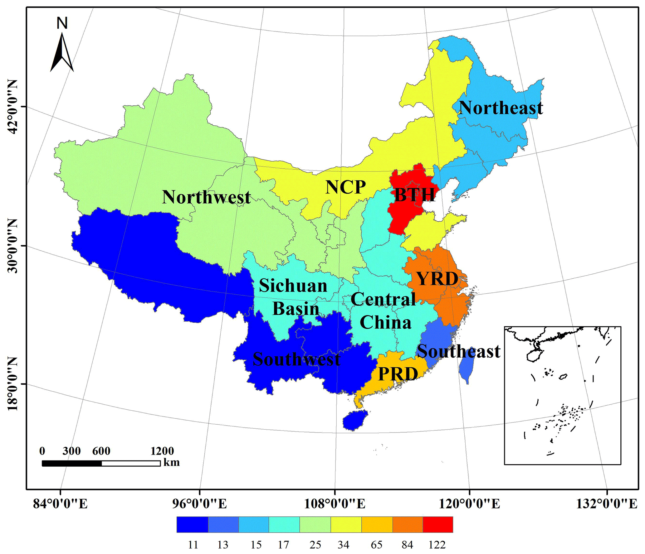
Figure 1Map of regions defined in this study (see Table S2 for provinces covered by each region). Color bar indicates the number of studies evaluating the region (studies covering all of China were excluded from counting). Publisher's note: please note that the above figure contains disputed territories.
2.2 Metrics evaluated
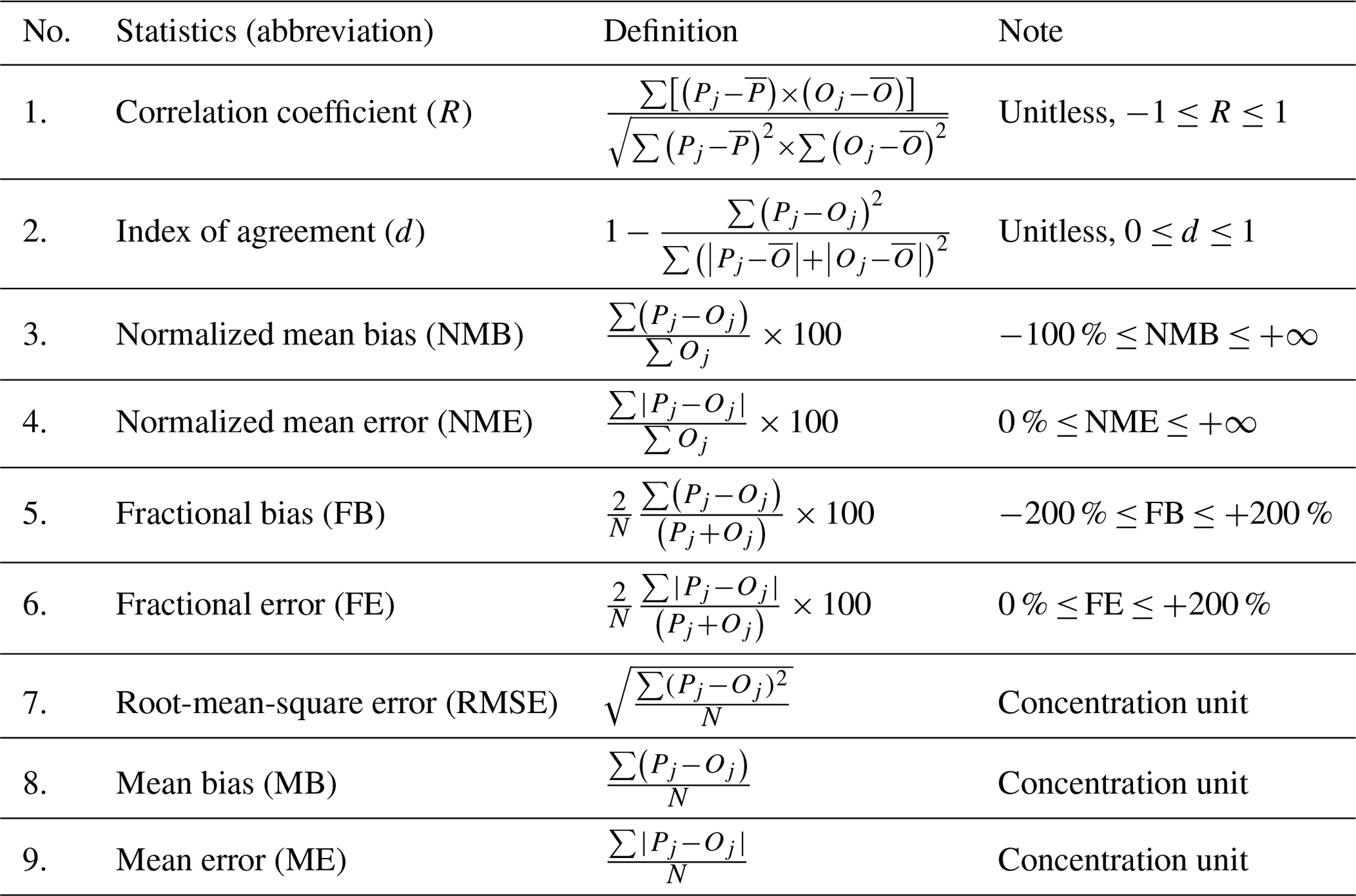
A total of 25 performance metrics were used in the 307 articles compiled in this study (see Supplement Table S4 for a complete list of the 25 metrics). In general, these statistical metrics could be divided into two types: one is to indicate how well models capture the magnitude of observations. Examples of this type include mean bias (MB), normalized mean bias (NMB), and fractional bias (FB). The other type of statistical metrics is used to indicate how models capture the variations in observations, where the most commonly used metrics are “correlation coefficient” or “index of agreement”. While some of the compiled studies explicitly provide mathematical formulas for the MPE metrics used in their papers, many did not. This causes ambiguity when a common terminology or abbreviation is used but no explicit formula is provided. For example, the term of correlation coefficient (or “correlative coefficient”) is frequently used in many studies but calculated using different mathematical formulas. In some studies the correlation coefficient refers to the Pearson correlation coefficient (R), which indicates the strength of linear relationship between observations and predictions, while in other studies it refers to the coefficient of determination (R2) that represents the fractions of predicted variations explained by observations. In these two cases, R2 is simply the square of R, yet the square root of R2 may be , where negative values are possible (indicating anti-correlation) and thus lead to ambiguity. In two studies (Wang et al., 2018; Zhang et al., 2018), the term correlation coefficient is used but formulated as the root-mean-square error (RMSE). To make things even more complicated, the correlation coefficient is used to indicate a model's ability to capture temporal variations in most of the studies but also spatial variations in some cases (e.g., Ge et al., 2014). For temporal variations, correlation coefficient is calculated based on temporally (hourly or daily) matched observation and modeled results at a single monitoring site (or averages across multiple monitoring sites in many cases). For spatial variations, correlation coefficient is calculated based on pairs of observations and modeled results at multiple sites, and its value is used to demonstrate spatial performance. For better comparability among studies, we converted R2 values to R (assuming always positive values). Index of agreement (IOA) is another example where caution must be taken since the definition of IOA is not unique among these studies. Most of the studies use the definition of IOA (d) shown in Table 1, yet one study used the formula in Table 3. The use of IOA is discussed more in Sect. 3.4, and we dropped the second formula for developing IOA benchmarks.
Table 1Definition of statistical metrics used in more than 10 studies complied in this work.
2.3 Derivation of benchmarks
In this study, the method established by Simon et al. (2012) and Emery et al. (2017) was mostly adopted. The quartile distribution for each statistical metric (depending on the data availability) is first presented and the influences of several model key inputs on these metrics are discussed. Rank-ordered distributions for selected metrics were then used to pick out the 33rd and 67th percentiles. According to Emery et al. (2017), the 33rd and 67th percentile separate the whole distribution into three performance ranges: studies that fall within the 33rd percentile successfully meet the goals that the best performing models are currently expected to achieve, studies that fall between 33rd and 67th quantiles successfully meet the criteria that the majority of modeling studies achieve, and studies that fall outside the 67th quantile indicate relatively poor performance for that specific metric. A summary table with values of 33rd and 67th quantile values for recommended statistical metrics is provided at the end of this work and is compared with US benchmarks proposed by Emery et al. (2017).
2.4 Feature importance based on random forest
Random forest is a machine learning method suitable for classification and regression (Liu et al., 2012). It is a collection of a series of decision trees, and each tree is generated from a bootstrap sample. Both continuous and categorical input variables are allowed. It can provide the order of feature importance (FI) so that we can determine and rank which parameter choices most influence the simulation results.
We reviewed the model configurations for studies that reported correlation
coefficient, IOA, MB, NMB, mean error (ME), normalized mean error (NME),
fractional bias (FB), and fraction error (FE) for PM2.5 (a total of 176 studies). Model configurations include the meteorological data that are used
to drive air quality simulations (e.g., from WRF, MM5, or GEOS), the emission
inventory (e.g., publicly available dataset vs. locally developed dataset), gas-phase
chemistry (for example, carbon bond vs. Statewide Air Pollution Research
Center (SAPRC)), aerosol chemistry (including inorganic aqueous chemistry,
inorganic gas-particle partitioning, and organic gas-particle partitioning and
oxidation), boundary conditions (e.g., model default values vs. results
generated from global model), grid resolution, and temporal resolution
(Table S7). We ignored the study region and period for FI selection because
these two options are more restricted by the user's specific needs and focus
(i.e., more subjective and uncontrollable and less objective and controllable). We
ranked each statistical metric from good to poor performance. For example,
values of R and IOA that are close to 1 represent good performance, and
values close to 0 represent poor performance. For MB and NMB, we used
absolute values so that deviations from zero represent the performance
level. These results were classified into three tiers with breaks at 33 %
and 67 % of the ranked values so that each tier includes the top third, the middle third, and the bottom third of the reported
performance results. The random forest model was performed using the
sklearn module in Python to obtain the FI metric.
3.1 General overview of air quality modeling studies in China
A total of 307 articles with AQM applications published between 2006 and 2019 were compiled in this work. Figure 2a shows the number of articles published in each year during the past 14 years. Prior to 2013, the number of studies that utilized AQMs in China was generally limited. A noticeable increase in the number of studies was apparent in 2013, with a doubling or tripling each year during 2016–2019. This sharp increase coincides with the infamous record-breaking haze event in January and December 2013 that attracted widespread attention to air pollution issues in China. Since then, a series of air-pollution-related actions were carried out due to the increasing funding that became available to the research community. Of the 307 articles included in this work, CMAQ was the most frequently used AQM (used in 124 studies), followed by WRF-Chem (111 studies), CAMx (36 studies), GEOS-Chem (20 studies), and NAQPMS (18 studies). Several studies evaluated model performance for multiple models (e.g., Wu et al., 2012; Zhang et al., 2016; Wang et al., 2017). In terms of regions, BTH (122 studies), YRD (84 studies), and PRD (65 studies) are the top three most evaluated regions (Fig. 1) (note that we excluded studies that cover the entirety of China for this count).
Meteorological data are needed to drive air quality simulations, and the performance of meteorological modeling is a key source of uncertainty for air quality modeling performance. Meteorological data were mostly simulated by the Weather Research Forecasting (WRF) model (Skamarock et al., 2005) in our compiled studies; the Fifth Generation Penn State/NCAR Mesoscale Model (MM5) (Grell et al., 1994) and the Regional Atmospheric Modeling system (RAMS) were used in a few studies. Model performance of meteorological results should be evaluated in addition to air quality simulation results. However, several studies did not report any results with respect to their meteorological simulations. The performance of meteorological results used to drive air quality simulations and how it could affect the air quality simulations is beyond the scope of the current work and will need to be discussed as a future work.
Emission inventories are another critical input for AQM applications, and their accuracy certainly affects the model performance. The most frequently used emission inventories for anthropogenic sources include the MEIC developed by Tsinghua University (http://www.meicmodel.org, last access: 25 December 2020), Regional Emission Inventory in Asia (REAS, Kurokawa et al., 2013), Intercontinental Chemical Transport Experiment-Phase B (INTEX-B) emissions (Zhang et al., 2009), MIX Asian anthropogenic emissions developed by the Model Inter-Comparison Study for Asia (MICS-Asia) emission group (Li et al., 2017), and many locally developed emission inventories at regional or city scales. For biogenic emissions, the Model of Emissions of Gases and Aerosols from Nature (MEGAN, Guenther et al., 2006) was the dominant source of information.
The national monitoring stations from the China National Environmental Monitoring Center (CNEMC) are the dominant observational data source used for model validation. The coverage of the national monitoring system increased from 74 major cities in 2013 to 337 cities across China in 2018. However, since only criteria pollutants (namely PM2.5, PM10, SO2, O3, NO2, and CO) are routinely measured at the national monitoring sites, model validation for speciated PM2.5, ammonia, and volatile organic compounds (VOCs) species (e.g., isoprene, formaldehyde) can only be based on measurements obtained from local monitoring sites or field observations conducted by individual research groups.
Figure 2b shows the reporting frequency for each statistical metric compiled in this study. Table 1 shows the formula of metrics that have been used in more than 20 studies. Same as Simon et al. (2012), the top three most frequently used metrics is correlation coefficient (R, 223 studies), normalized mean bias (NMB, 170 studies), and mean bias (MB, 132 studies). Other frequently used (>20 studies) metrics include root mean square error (RMSE, 118 studies), normalized mean error (NME, 111 studies), fractional bias (FB, 66 studies), fractional error (FE, 62 studies), index of agreement (IOA, 57 studies), and mean error (ME, 27 studies). NMB and NME were only used in 15 and 10 studies, respectively, since as mentioned in Simon et al. (2012) these two metrics tend to give more weight to data at low values. About 65 % of the articles included in this work used at least three statistical metrics for model performance evaluation (Fig. 2c), 16 % of studies reported numerical values for only one metric, less than 10 % of studies included more than five MPE metrics, and four studies (Li et al., 2015; Kim et al., 2017; Li et al., 2018; Zhang et al., 2017) used eight statistical metrics. In terms of number of pollutants evaluated in each study (Fig. 2d), 132 studies (43 %) evaluated only one pollutant, and 223 studies (73 %) evaluated less than or equal to three pollutants, while one study (Ying et al., 2018) evaluated 17 pollutants (including elemental PM2.5 components).
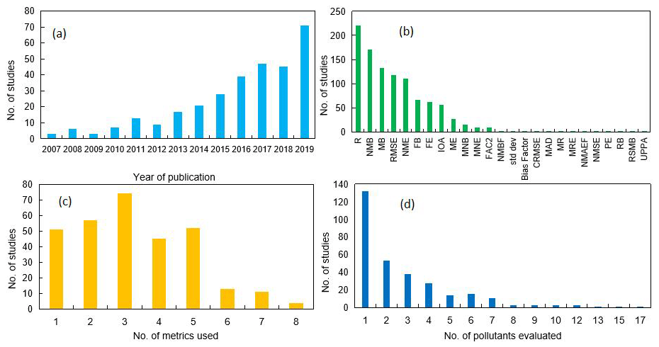
Figure 2(a) Number of studies published during 2006–2019, (b) frequency of the use of each metric, (c) number of metrics used in studies, and (d) frequency of number of pollutants evaluated.
Figure 3 shows the number of studies broken down by pairs of pollutants and AQM models and pairs of pollutants and metrics. As expected, PM2.5 is the most frequently evaluated pollutant, followed by ozone, NO2, SO2, and PM10, all of which are criteria pollutants included in China's National Ambient Air Quality Standards (NAAQS). Evaluation of speciated PM species, including nitrate, sulfate, ammonium, and organic carbon (OC) is about 25 % less frequent than total PM2.5 and was only covered in applications for certain regions due to limited observations.
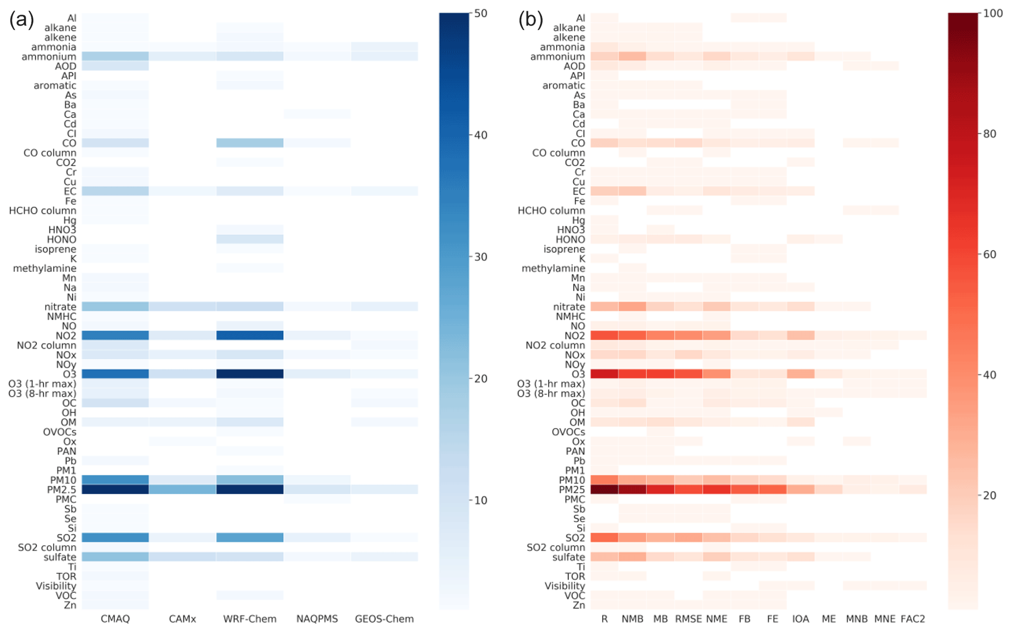
Figure 3Number of studies evaluating each pollutant and AQM model pair (a). Number of studies evaluating each pair of a pollutant and statistical metric (b). See Table S5 for species abbreviations.
3.2 Quantile distributions of PM2.5 and speciated components
Figure 4 shows quantile distributions for the eight most frequently used model performance metrics for PM2.5 and speciated components (corresponding values are listed in Table S5). For total PM2.5, slightly more negative values of MB, NMB, and FB were reported. Absolute bias for PM2.5 ranged from as low as −50 µg m−3 to over 50 µg m−3 (outliers excluded) with median values around 3 µg m−3. The bias range for speciated components was much smaller (within 20 µg m−3) because the absolute magnitude of speciated components was much smaller. In terms of the normalized bias (i.e., NMB and FB), the range of PM2.5 was comparable or smaller than speciated components, partly due to the compensating errors from speciated components. Speciated PM2.5 tended to be dominantly underestimated except for nitrate (in terms of NMB) and elemental carbon (EC; in terms of FB). The widest range of normalized bias was reported for nitrate, suggesting substantial uncertainties in simulated nitrate concentrations. Some early reported large negative NMB values of nitrate were partly due to missing formation of coarse-mode nitrate implemented in early version of the model (Kwok et al., 2010). As the model evolved over time and emission inventories improved, the large negative bias of nitrate disappeared (see Fig. S3). Speciated PM components can be both emitted directly from sources (i.e., primary) and formed via chemical reactions of precursors (i.e., secondary). Model underestimates of secondary species (organic and inorganic) have been reported in numerous studies with explanations ranging from missing formation mechanisms, to uncertainties with the emission inventory and meteorological errors. EC is solely emitted from sources; thus, the performance of simulated EC concentrations is strictly associated with the accuracy of the emission inventory and meteorological mixing and transport.
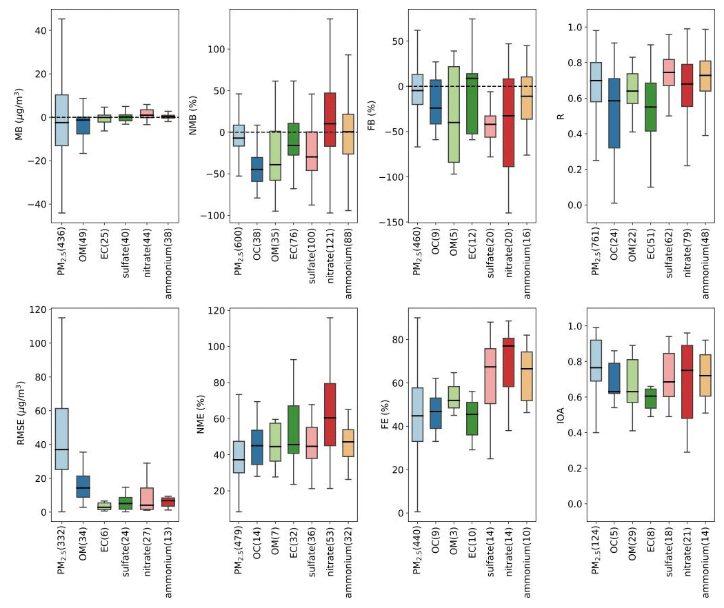
Figure 4Quantile distribution of selected PM performance metrics compiled in this work. Median values are shown as centerlines, the upper and lower bound of boxes correspond to the 25th and 75th percentile values, and whiskers extend to 1.5 times the interquartile range (outliers are excluded). The numbers in brackets indicate the number of data points available.
For error metrics, total PM2.5 performed better than speciated components in terms of NME, with a median NME value around 40 %. For FE, median values for total PM2.5 and carbonaceous species were within 4 %–60 %, while inorganic secondary species had relatively large (>60 %) median FE.
R and IOA are used to indicate how well the model could capture the variations of observed values, and both values are within the range of 0–1. We converted R2 values to R for better comparability. For total PM2.5, the median IOA was 0.76, while median R was 0.69 (R2=0.4761). The minimum IOA value reported for total PM2.5 was 0.4, while the minimum R value could be negative. A total of 11 studies reported both R and IOA values, which enabled intercomparisons of the two metrics based on identical sets of data points. It was found that IOA values always tend to be higher than R values (38 out of 40 data pairs). Compared to total PM2.5, secondary inorganic aerosols (i.e., sulfate, nitrate, and ammonium) demonstrated better performance in terms of R values but slightly poorer performance in terms of IOA values. OM and EC show lower values for both R and IOA compared to total PM2.5.
3.2.1 Impact of season
There are numerous factors that could affect model performance results, such as the study region and period, uncertainty of emission inventory, model grid resolution, the temporal resolution of paired observations, and modeling results used for model evaluation. We first looked at NMB results for total PM2.5 and selected species (due to availability of data points) by season (Fig. 5). For total PM2.5, the number of data points reported for winter is significantly higher than those reported for other seasons as heavy haze episodes generally occur in winter. Reported NMB for total PM2.5 was dominantly negative, except for winter where positive NMB was also reported. Most of the large positive NMB values (>50 %) reported for winter were from a single study (Zhang et al., 2017), for which the author explained that the overestimation may be associated with the inconsistency of emissions between the base year and the modeling year. Sulfate tended to be overwhelmingly underestimated regardless of season, which is commonly reported in the literature, potentially because of missing formation mechanisms (e.g., heterogeneous reactions, Ye et al., 2018; Huang et al., 2019; Shao et al., 2019; Chen et al., 2019). However, a few large NMB values (>50 %) were reported in fall (Cheng et al., 2019). Nitrate and ammonium exhibited equivalent overestimations and underestimations for all seasons, and differences among seasons were minor. OM also tended to be more underestimated, especially in summer and fall. The underestimation of organic components, especially the secondary organic aerosols (SOA), was well documented by many studies (e.g., Jimenez et al., 2009; Q. Chen et al., 2017; Zhao et al., 2016). The two positive NMB values reported for winter were from one study (Li et al., 2018) ,and uncertainties in anthropogenic emissions were explained as the key source of model bias.

3.2.2 Impact of region
We also considered whether there are any regional differences in these statistical metrics. Constrained by number of data points, we only compared results of R and NMB for total PM2.5 and secondary inorganic species over three key regions in China (BTH, YRD, and PRD; Fig. 6). These three regions represent the most populated, economically developed, and urbanized city clusters in China. With respect to total PM2.5, R and NMB values for the three regions did not exhibit substantial differences. All three regions exhibited more negative NMB values with median NMB around −10 %. Reported R values for PRD were slightly lower compared with the other two regions. For sulfate and ammonium, reported R values for YRD were significantly lower than the other two regions. Underestimation of sulfate and ammonium was more severe in YRD and PRD. For nitrate, PRD showed the lowest R values, and model bias shifted from positive to negative as the target region got warmer.
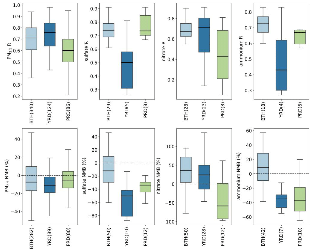
Figure 6Quantile distribution of R and NMB of total PM2.5 and speciated species in BTH, YRD, and PRD.
3.2.3 Impact of temporal and spatial resolution
Although AQMs are usually set to output data at hourly time steps, validation of modeling results is not always performed against hourly data, depending on the temporal resolution of observational data and the purpose of the application. Daily, monthly, and annually averaged pairs of model results and observations were used for model evaluation. Of the 307 studies compiled in this work, 183 (60 %) studies used hourly data for model validation, followed by 90 (29 %) using daily, 31 (10 %) using monthly, and 12 (4 %) using annual data. Due to the coarse temporal resolution of GEOS-Chem output in general, the finest GEOS-Chem validation was conducted using daily data. Figure 7 shows the quantile distribution of eight statistical metrics for total PM2.5 presented by the temporal resolution used for model validation (plots for speciated components are shown in Fig. S1; results for annual are not shown due to insufficient data). Model performance evaluated using daily-average values were similar or slightly better than hourly values but exhibited large improvements when monthly average values were used. For instance, reported R values did not show much difference at hourly and daily scales (median values around 0.7) but exhibited a substantial improvement at a monthly scale (median value around 0.85). A similar trend was also observed for reported error statistics (NME and FE), which showed slight improvement as the validation resolution increased from hourly to daily but a large improvement from daily to monthly. One study (Matsui et al., 2009) provided two sets of R values based on hourly and daily averaged data, and R values for daily averages were always higher (12 out of 14 values).
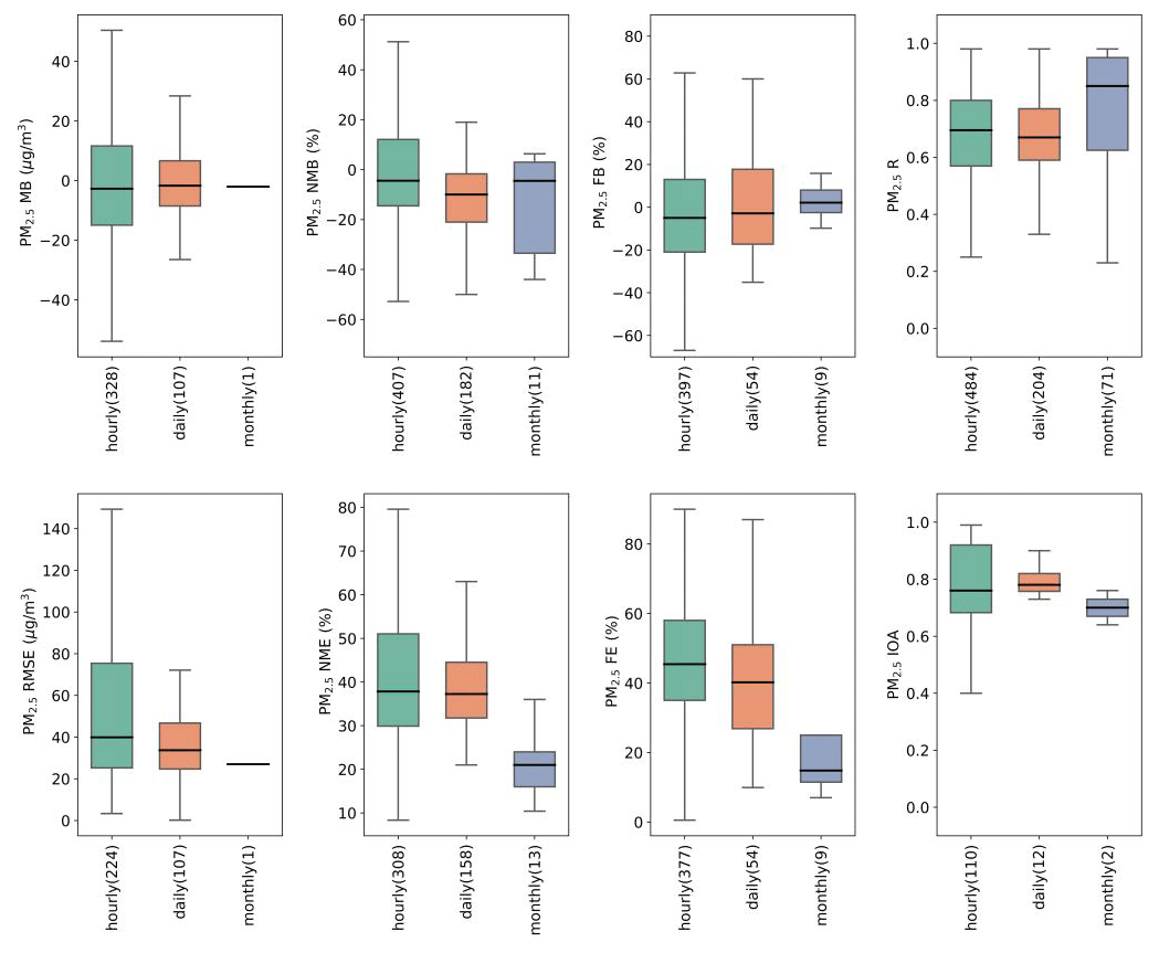
Figure 7Quantile distributions of MB, RMSE, NMB, NME, FB, FE, R, and IOA of total PM2.5 presented by temporal resolution for model validation.
Spatial resolution is key for AQM applications. For applications at local or urban scale, AQMs are usually configured with two or three nested domains, with downscaling from a coarser outer domain to finer inner domains. Among the 307 articles compiled in this study, a total of 43 grid resolutions were used (for nested grids, we used the grid solution from the finest grid), ranging from over 200 km (used by GEOS-Chem) to 1 km depending on the target region and the purpose of the application. GEOS-Chem was more often used with coarse resolution (>50 km). We classified these different grid resolutions into five categories: 0–5, 5–10, 10–25, 25–50, and 50–100 km. Figure 8 shows the distribution of eight statistical metrics for total PM2.5 by these four categories (plots for speciated components are shown in Fig. S2). It appears that finer spatial resolution did not necessarily improve model performance results. For example, the R values for the finest-resolution category ranged from as low as 0.47 to as high as 0.85, while for the coarsest category they ranged from 0.33 to 0.96. MB appeared to move from underestimation to overestimation from fine to coarse resolution but no clear trend was observed for FB and NMB. Reported NME and FE values also appeared to increase with coarser grid resolution. As mentioned above, many factors could affect model performance. Thus, it is difficult to solely evaluate whether there is a systematic improvement in model performance as the modeling resolution gets finer. While most of the studies only performed model evaluation for one modeling domain (usually the finest domain), a few studies (e.g., Qiao et al., 2015; Wang et al., 2015; X. Liu et al., 2010; S. Liu et al., 2018) calculated statistical results for multiple domains where results for finer spatial resolution were generally better than those for coarser resolution. For instance, Wang et al. (2015) reported results for hourly PM2.5 at two spatial resolutions (12 km vs. 36 km) simultaneously. For this particular study, the model overpredicted PM2.5 at 12 km resolution (positive values of MB, NMB, and FB) but underpredicted PM2.5 at 36 km resolution (negative values of MB, NMB, and FB). This is likely due to the dilution effect that makes model results lower at 36 km domain.
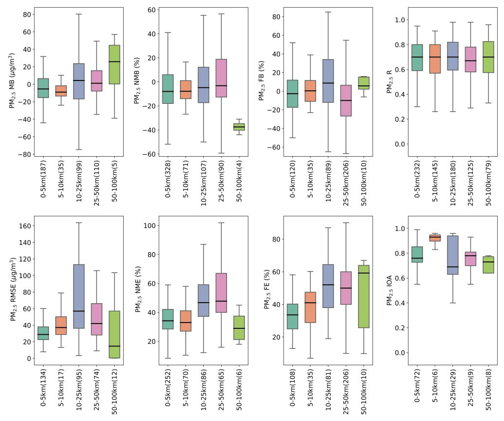
Figure 8Quantile distributions of MB, RMSE, NMB, NME, FB, FE, R, and IOA of total PM2.5 presented by model grid resolution.
Fine-resolution simulations have been conducted with the intention of improving model performance. With finer grid resolution, the spatial allocation of certain features in emission patterns is significantly improved, which is especially important for air quality simulations at local scale (Tan et al., 2015; Liu et al., 2020). Additionally, meteorological simulations could also be improved at finer resolution given more detailed land cover and structures in topography (Tao et al., 2020), which in turn improves the subsequent air quality simulations. Estimation of PM2.5-related health impacts are reported to be biased high or low at coarse spatial resolution (Li et al., 2016; Thompson and Selin, 2012). Lin et al. (2020) developed a new online regional atmospheric chemistry model, WRF-GC (v1.0), which integrates the WRF meteorology model and GEOS-Chem chemistry model. This new WRF-GC model has been configured with a spatial resolution of 27 km and successfully applied to quantify the changes of NOx emissions due to COVID-19 for eastern China (Zhang et al., 2020), illustrating the potential applications of GEOS-Chem at a finer spatial scale. However, not all fine-resolution simulations lead to improved model performance, especially when the input data are not available with the same high resolution (Jiang and Yoo, 2018; Tao et al., 2020). Therefore, grid resolution should be determined depending on the purpose of the study and the availability of input data.
3.2.4 Trends over the past decade
In an attempt to assess whether model performance results have evolved over the past decade, we present time series of selected statistical metrics for total PM2.5 in Fig. 9 (plots for inorganic species are shown in Fig. S3). Results published prior to 2013 were aggregated into one group because there were a limited number of studies prior to 2013. For total PM2.5, reported R values have remained relatively consistent over the past decade, with the median fluctuating within 0.6–0.8. The ranges of reported RMSE and MB have become narrower in recent years even though the number of studies has increased substantially. Reported IOA and RMSE values fluctuated upward and downward over the period. On the other hand, there seems to be an improving trend in terms of FB, FE, and NME as the reported values for these three metrics shift towards zero. For instance, the median value of reported FE decreased from 56.9 % prior to 2013 to around 33 % in 2019. However, it is important not to overinterpret these results, as the number of studies published each year could affect the results.
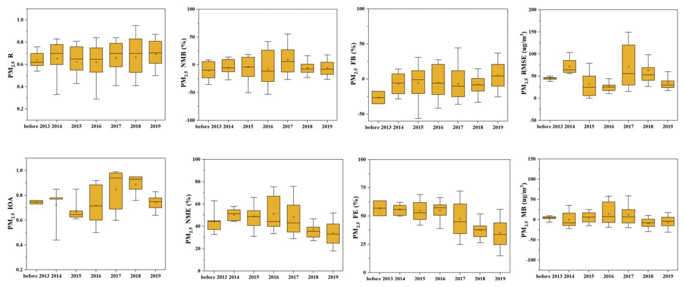
Figure 9Quantile distribution of R, IOA, NMB, NME, FB, FE, MB, and RMSE of total PM2.5 presented by data published year.
3.3 Recommended metrics and benchmarks
We present diagrams to develop metrics and benchmarks for model evaluation. Figure 10 shows the rank-ordered distribution of R, IOA, NMB, NME, FB, and FE results for total PM2.5 and speciated components from all studies compiled in this work. Results of R for total PM2.5 are further split into hourly (h), daily (d), and monthly (m) resolution since R increases as temporal resolution changes from hourly to monthly. The top 33rd percentile value increases from around 0.76 for hourly and daily to 0.92 for monthly results; the top 67th percentile increases from 0.60–0.70 as the total PM2.5 is evaluated with coarser resolution. Secondary inorganic species (sulfate, nitrate and ammonium) show similar range (0.65–0.75) over the 33rd to 67th percentile interval. For OC/OM and EC, the 33rd and 67th percentile R value is lower compared to inorganic species; the 33rd to 67th percentile for OC/OM is 0.56–0.69 for OC/OM and 0.48–0.65 for EC. In terms of IOA, the 33rd to 67th percentile interval ranges from 0.73–0.83 for total PM2.5 and lower for speciated components. Values for EC were not shown due to insufficient data. For bias and error, total PM2.5 exhibits smaller values compared with speciated components, due to potential compensating effects from different components. The 33rd percentile of absolute NMB for total PM2.5 is less than 10 %, while the 67th percentile is less than 20 %. Among the three secondary inorganic species, the bias and error of nitrate exhibits largest variability (NMB ranges from 17.0 %–55.2 % and NME from 47.0 %–71.2 % for the 33rd to 67th percentile interval). The 33rd to 67th range of NMB for EC (16.0 %–32.4 %) is much lower than that for OC/OM (34.7 %–55.0 %), while NME for OC/OM and EC is similar, ranging from ∼ 40 %–55 %. The number of FB and FE data is considerably lower than NMB and NME for speciated components, and nitrate exhibits the largest variability in terms of FB and FE.
Based on our analysis and previous conclusions from Emery et al. (2017), we propose recommended statistical metrics and associated benchmarks for total PM2.5 and speciated component as shown in Table 2. Bolded values indicate that less than 20 data points were available to develop the benchmarks. Values for goal indicate that roughly the top third of studies represents the best that models are currently expected to achieve. Values for criteria indicate that roughly the top two-thirds of studies represent results from the majority of studies. Based on our results, NMB for total PM2.5 should be within 10 % and 20 % if the goal and criteria benchmark is to be met; corresponding values for NME are 35 % (goal) and 45 % (criteria). In terms of R, our recommended benchmarks range from 0.60 to 0.70 for hourly and daily PM2.5 and 0.70 to 0.90 for monthly PM2.5. The recommended benchmark value for IOA is 0.80 for goal and 0.70 for criteria. Our table differs from Emery et al. (2017) in three aspects. First, we add benchmarks for IOA in addition to the correlation coefficient. We found a general increasing trend in using IOA for model performance evaluation since 2013 (prior to 2013, only six of our compiled studies used IOA; after 2013, 51 studies used IOA). Second, we present benchmarks for different temporal resolution for total PM2.5 when possible. As mentioned above, reported R values for total PM2.5 improve with coarser temporal resolution, while no strong trend is observed for other metrics. Third, Emery et al. (2017) did not present benchmarks for the correlation coefficient of speciated PM components due to large uncertainties and insufficient data. Here we present benchmarks for R and IOA for speciated PM components (except for EC IOA), but caution should be taken comparing to these benchmarks. For example, less than 20 data points were used to develop the IOA benchmarks for ammonium and sulfate. For those compounds, we do not observe sudden shifts in the rank order distribution as observed in Emery et al. (2017). Thus, we keep these values for future reference. For bias and error metrics, we do observe sharp changes in rank order values, for example, in the NMB/FB for nitrate, and FB for EC. Therefore, we do not give benchmarks for these. We also present benchmarks for FB and FE.
Table 2Recommended benchmarks for evaluating AQM applications in China for total PM2.5 and speciated componentsa,b.
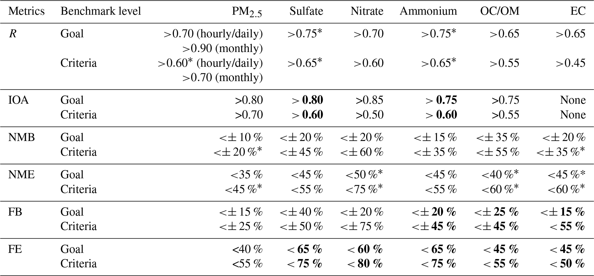
a Values with an asterisk in Table 2 indicate that our benchmarks are stricter than corresponding values in Emery et al. (2017). b Bolded values indicate that less than 20 data points were available to develop the benchmarks.

We further compare our results with benchmarks for the US proposed by Emery et al. (2017). Values with an asterisk in Table 2 indicate that our benchmarks are stricter than corresponding values in Emery et al. (2017), which means it would be more difficult for results from a particular study to attain our recommended 33rd (or 67th) percentiles. For total PM2.5, our proposed benchmarks are generally stricter than that in Emery et al. (2017). For example, our NMB (NME) criteria value for PM2.5 is 20 % (45 %) as opposed to 30 % (50 %) in Emery's study; the criteria value for the R benchmark is also higher (0.60) than those based on US1 studies (0.40). This might partially reflect the systematic improvements in model applications (e.g., incorporation of newly discovered mechanisms) during the past several years as the latest study included in Emery et al. (2017) was published in 2015. Our goal values for NMB, NME, and R benchmarks are the same as those proposed by Emery et al. (2017). For speciated components, NME benchmarks for nitrate are lower (i.e., stricter) than Emery's study, while the opposite is true for sulfate and ammonium. For correlation coefficient, our criteria benchmarks for sulfate and ammonium (0.65) are much higher (i.e., more strict) than those in Emery's study (0.40).
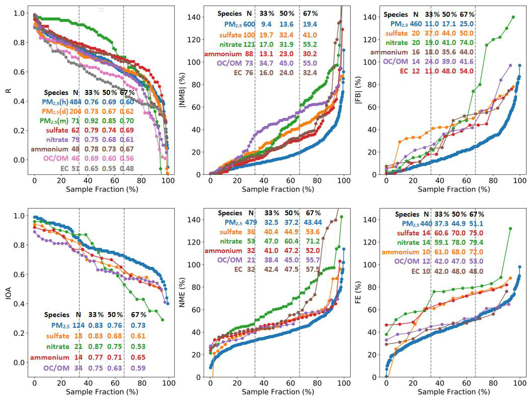
Figure 10Rank-ordered distributions of R, IOA, NMB, NME, FB, and FE for total PM2.5 and speciated components. The number of data points and the 33rd, 50th, and 67th percentile values are also listed. For instance, one-third of the reported R values for predicted hourly PM2.5 concentration are higher than 0.76, half are higher than 0.69, and two-thirds are higher than 0.60.
As mentioned earlier, AQM applications involve numerous driving inputs and diverse model configurations, which lead to an abundant database from which to assess their relative influences on model performance. The similarities between the benchmarks derived in this study and Emery's study suggest that important model input data (e.g., emission inventories) have comparable accuracy for China and North America, and model formulations (e.g., algorithms such as chemistry, deposition, and transport) seem to be equally applicable to China and North America. In addition to the need for model performance benchmarks, there also is a need for more studies that quantify contributions to model uncertainty, such as the recent study by Dunker et al. (2020), which quantifies contributions of chemistry, boundary concentrations, deposition, and emissions to uncertainty in simulated ozone results. In this study, we applied the random forest method for pattern recognition to identify and rank model attributes (inputs, grid resolutions, etc.) that have important influences on PM2.5 model performance. The choice of emission inventory is shown to affect the model performances most, followed by grid resolution, aerosol, and gas chemistry (Fig. 11). Meteorological input and the choice of model itself is of least importance.
3.4 Additional discussions and recommendations
3.4.1 Benchmarks for the European modeling community – FAIRMODE
The air quality model benchmarking practice for AQM applications by the FAIRMODE community is somewhat different from the US benchmarks. The main modeling performance indicator is called the modeling quality indicator (MQI), which is calculated based on RMSE and measurement uncertainties (function of mean value and standard deviation of observations) (Janssen et al., 2017). The modeling quality objective (MQO) is the criteria value for MQI and is said to be met if MQI is less than or equal to one. In addition to the main MQI, three statistical indicators that describe certain aspects of the differences between observed and modeled results – namely bias, correlation, and standard deviation are proposed as the modeling performance indicators (MPI). For each MPI, the model performance criterion (MPC) that individual MPI is expected to meet is also given. However, unlike fixed values given in this study and Emery et al. (2017), MPC is dependent on observation uncertainties. Therefore, it is not directly comparable between MPC and the benchmarks proposed in this study or those in Emery et al. (2017).
3.4.2 The use of “index of agreement”
The concept of index of agreement was originally proposed by Willmott in the 1980s and has since then been widely used to “reflect the degree to which the observed variate is accurately estimated by the simulated variate” (Willmott, 1981) in a variety of fields. IOA has gone through several modifications (together referred as Willmott indices) since it was proposed in the original formula (Willmott, 1982; Willmott et al., 1985, 2012). The formula of the original form (d) is shown in Table 2 (presented again in Table 3) and the other three (d1, , and dr) are shown in Table 3. The first version of IOA is proposed over the correlation coefficient for its ability to “discern differences in proportionality and/or constant additive differences between the two variables” (Willmott, 1981), and this version is also the most widely used version in our compiled studies. Compared with R2 values, the original IOA results in systematically higher values (Valbuena et al., 2019) and thus is being adopted in an increasing number of studies partially because it makes results appear “better”. However, the original and most widely-used formula is problematic in that too much weight is given to the large errors when squared (Willmott et al., 2012) and relatively high IOA values could be obtained even when a model is performing poorly (Willmott et al., 1985; Pereira et al., 2018). Newer versions as later proposed by Willmott overcome this problem by removing the squaring and are recommended over the original one (Willmott et al., 1985, 2012).
Nearly 20 % (57 studies) of our compiled studies used the original IOA formulation for MPE, but only one study (Peng et al., 2011) used the second formula (d1). Since there is an increasing trend of using the original IOA formula as a model performance indicator for AQM applications in China (prior to 2013 only 6 study vs. 51 studies after 2013), we decided to keep IOA for future reference, but caution should be taken when using and interpreting IOA values. It should be noted that IOA alone does not necessarily indicate how well the model performs.

3.4.3 Additional recommendations
Other than the recommended metrics and associated benchmarks listed in Table 2, we list additional recommendations for validation practices that would enable a complete and comprehensive picture of model performance.
-
Provide explicit mathematical formulas for statistical metrics being used to avoid any confusion. As mentioned earlier, many studies did not give explicit formulas, which caused ambiguity when a common name (for example, correlation coefficient, or index of agreement) was used but calculated in numerous ways.
-
Provide as much detail as possible with respect to how observation and modeling results are used to obtain the statistical results. For example, list how observed data and modeled results are paired in space and time, specify if averaging is performed prior to calculating statistical metrics, and specify the number of observation sites and the number of available data points being used. As Emery et al. (2017) note, statistics calculated over very large sets of observation–model pairings usually result in better statistics, but rarely convey useful information.
-
Meteorological information is an essential input to each air quality simulation (along with emissions, boundary concentrations, etc.) and uncertainties in the meteorology will inevitably influence the air quality simulation to some degree. Indeed, meteorological errors could be offset by errors in other model inputs thus resulting in good air quality performance evaluation results for the wrong reasons (Reynolds et al., 1996). For example, the effect of low-biased wind speed could be offset by low-biased emissions or vice versa, producing simulated air quality in agreement with observations but an incorrect response of air quality to emission changes. Therefore, evaluating the meteorological model performance is as important as air quality model performance evaluation. Present meteorological model performance results from good practices, usually including but not limited to temperature, humidity, wind speed, and wind direction. Performance results from meteorological modeling help to explain potential causes of unsatisfactory AQM results.
-
Include two types of statistical metrics for model evaluation, one to assess errors in magnitude (e.g., MB, NMB, or FB) and one to assess agreement in variation (e.g., R or IOA). Caution is needed when presenting values for normalized metrics, for example NMB or NME and FB or FE. Always express these in percentage to avoid ambiguity in whether normalized metrics are in decimal or percentage formats.
-
Evaluate multiple precursor and/or component pollutants, even if the study focuses on a single pollutant. Remain aware that opposing biases among speciated PM components may compensate each other and falsely indicate good performance for composite species such as total PM2.5.
-
In addition to listing statistical results, graphs and plots are strongly recommended to further support model validation. To give a few examples, visualizing data via time series and regression plots of modeled vs. observed data helps to illustrate periods and concentration ranges, respectively, with better or poorer performance. Spatial plots that include modeling results as background isopleths and observation data overlaid help illustrate how the model performs spatially.
With the increasing number of AQM applications in China over the past decade, a review of model performance is needed to help understand how well these models are currently performing compared with observations and how reliable future model applications are compared with existing studies. Following an established method used in the US, a total of 307 peer-reviewed studies that applied AQMs in China were compiled in this work, and key information, including model applied, study region, grid resolution, and evaluated metrics, was tabulated. Operational MPE results for total PM2.5 and speciated components reported in the compiled literature are presented in this study. Quantile distributions of common statistical metrics reported in the literature were presented and the impacts of different model configurations, including study region, study period, spatial and temporal resolutions on performance results are discussed. With the concept of “goals” and “criteria”, we proposed benchmarks for six commonly used metrics, NMB, NME, FB, FE, R, and IOA, based on the method employed by Emery et al. (2017). For total PM2.5, we provided R benchmarks with different temporal resolutions; for component species, we did not split results by temporal resolution due to an insufficient number of data points. We included results for IOA while recognizing that this specific metric should be used and interpreted with caution. Additional recommendations on good evaluation practices are provided. Results from this study help the ever-growing modeling community in China to put their model performance in context relative to previous studies and to guide modellers to conduct model evaluation in a more consistent fashion.
All data is available upon request from the corresponding author.
The supplement related to this article is available online at: https://doi.org/10.5194/acp-21-2725-2021-supplement.
LH performed the data analysis and prepared the manuscript with contributions from all co-authors. LL formulated the research goals and edited the manuscript. YZ, HZ, SX, TZ, and YS complied articles and collected data with equal contributions. LH and YZ reviewed and analyzed the collected data. CE, GY, and JF contributed to academic discussions and review.
The authors declare that they have no conflict of interest.
This article is part of the special issue “Regional assessment of air pollution and climate change over East and Southeast Asia: results from MICS-Asia Phase III”. It is not associated with a conference.
This study was financially sponsored by the National Natural Science Foundation of China (grant no. 42005112), the Shanghai Sail Program (no. 19YF1415600), the Shanghai Science and Technology Innovation Plan (no. 19DZ1205007), the National Natural Science Foundation of China (nos. 42075144, 41875161), the Shanghai International Science and Technology Cooperation Fund (no. 19230742500), and Chinese National Key Technology R&D Program (no. 2018YFC0213800).
This research has been supported by the National Natural Science Foundation of China (grant nos. 42005112, 42075144, and 41875161), the Shanghai Sail Program (no. 19YF1415600), the Shanghai Science and Technology Innovation Plan (no. 19DZ1205007), the Shanghai International Science and Technology Cooperation Fund (no. 19230742500), and Chinese National Key Technology R&D Program (no. 2018YFC0213800).
This paper was edited by Yafang Cheng and reviewed by three anonymous referees.
Boylan, J. W. and Russell, A. G.: PM and light extinction model performance metrics, goals, and criteria for three-dimensional air quality models, Atmos. Environ., 40, 4946–4959, https://doi.org/10.1016/j.atmosenv.2005.09.087, 2006.
Chen, D., Liu, X., Lang, J., Zhou, Y., Wei, L., Wang, X., and Guo, X.: Estimating the contribution of regional transport to PM2.5 air pollution in a rural area on the North China Plain, Sci. Total Environ., 583, 280–291, https://doi.org/10.1016/j.scitotenv.2017.01.066, 2017.
Chen, L., Gao, Y., Zhang, M., Fu, J. S., Zhu, J., Liao, H., Li, J., Huang, K., Ge, B., Wang, X., Lam, Y. F., Lin, C.-Y., Itahashi, S., Nagashima, T., Kajino, M., Yamaji, K., Wang, Z., and Kurokawa, J.: MICS-Asia III: multi-model comparison and evaluation of aerosol over East Asia, Atmos. Chem. Phys., 19, 11911–11937, https://doi.org/10.5194/acp-19-11911-2019, 2019.
Chen, Q., Fu, T. M., Hu, J., Ying, Q., and Zhang, L.: Modelling secondary organic aerosols in China, Natl. Sci. Rev., 4, 806–809, https://doi.org/10.1093/nsr/nwx143, 2017.
Cheng, J., Su, J., Cui, T., Li, X., Dong, X., Sun, F., Yang, Y., Tong, D., Zheng, Y., Li, Y., Li, J., Zhang, Q., and He, K.: Dominant role of emission reduction in PM2.5 air quality improvement in Beijing during 2013–2017: a model-based decomposition analysis, Atmos. Chem. Phys., 19, 6125–6146, https://doi.org/10.5194/acp-19-6125-2019, 2019.
Dunker, A. M., Wilson, G., Bates, J. T., and Yarwood, G.: Chemical Sensitivity Analysis and Uncertainty Analysis of Ozone Production in the Comprehensive Air Quality Model with Extensions Applied to Eastern Texas, Environ. Sci. Technol., 54, 5391–5399, https://doi.org/10.1021/acs.est.9b07543, 2020.
Emery, C., Liu, Z., Russell, A. G., Odman, M. T., Yarwood, G., and Kumar, N.: Recommendations on statistics and benchmarks to assess photochemical model performance, JAPCA J. Air. Waste Ma., 67, 582–598, https://doi.org/10.1080/10962247.2016.1265027, 2017.
EPA: Guideline for regulatory application of the Urban Airshed Model (No.PB-92-108760/XAB). Environmental Protection Agency, Research Triangle Park, NC, USA, 1991.
Feng, S., Jiang, F., Jiang, Z., Wang, H., Cai, Z., and Zhang, L.: Impact of 3DVAR assimilation of surface PM2.5 observations on PM2.5 forecasts over China during wintertime, Atmos. Environ., 187, 34–49, https://doi.org/10.1016/j.atmosenv.2018.05.049, 2018.
Foley, K. M., Roselle, S. J., Appel, K. W., Bhave, P. V., Pleim, J. E., Otte, T. L., Mathur, R., Sarwar, G., Young, J. O., Gilliam, R. C., Nolte, C. G., Kelly, J. T., Gilliland, A. B., and Bash, J. O.: Incremental testing of the Community Multiscale Air Quality (CMAQ) modeling system version 4.7, Geosci. Model Dev., 3, 205–226, https://doi.org/10.5194/gmd-3-205-2010, 2010.
Gao, J., Zhu, B., Xiao, H., Kang, H., Hou, X., Yin, Y., Zhang, L., and Miao, Q.: Diurnal variations and source apportionment of ozone at the summit of Mount Huang, a rural site in Eastern China, Environ. Pollut., 222, 513–522, https://doi.org/10.1016/j.envpol.2016.11.031, 2017.
Gao, M., Ji, D., Liang, F., and Liu, Y.: Attribution of aerosol direct radiative forcing in China and India to emitting sectors, Atmos. Environ., 190, 35–42, https://doi.org/10.1016/j.atmosenv.2018.07.011, 2018.
Ge, B. Z., Wang, Z. F., Xu, X. B., Wu, J. B., Yu, X. L., and Li, J.: Wet deposition of acidifying substances in different regions of China and the rest of East Asia: Modeling with updated NAQPMS, Environ. Pollut., 187, 10–21, https://doi.org/10.1016/j.envpol.2013.12.014, 2014.
Grell, G. A., Dudhia, J., and Stauffer, D. R.: A description of the fifth-generation Penn State/NCAR mesoscale model (MM5), University Corporation for Atmospheric Research, https://doi.org/10.5065/D60Z716B, 1994.
Grell, G. A., Peckham, S. E., Schmitz, R., McKeen, S. A., Frost, G., Skamarock, W. C., and Eder, B.: Fully coupled “online” chemistry within the WRF model, Atmos. Environ., 39, 6957–6975, https://doi.org/10.1016/j.atmosenv.2005.04.027, 2005.
Guenther, A., Karl, T., Harley, P., Wiedinmyer, C., Palmer, P. I., and Geron, C.: Estimates of global terrestrial isoprene emissions using MEGAN (Model of Emissions of Gases and Aerosols from Nature), Atmos. Chem. Phys., 6, 3181–3210, https://doi.org/10.5194/acp-6-3181-2006, 2006.
Hu, J., Li, X., Huang, L., Ying, Q., Zhang, Q., Zhao, B., Wang, S., and Zhang, H.: Ensemble prediction of air quality using the WRF/CMAQ model system for health effect studies in China, Atmos. Chem. Phys., 17, 13103–13118, https://doi.org/10.5194/acp-17-13103-2017, 2017.
Huang, L., An, J., Koo, B., Yarwood, G., Yan, R., Wang, Y., Huang, C., and Li, L.: Sulfate formation during heavy winter haze events and the potential contribution from heterogeneous SO2 + NO2 reactions in the Yangtze River Delta region, China, Atmos. Chem. Phys., 19, 14311–14328, https://doi.org/10.5194/acp-19-14311-2019, 2019.
Janssen, S., Guerreiro, C., Viane, P., Georgieva, E., Thunis, P., Cuvelier, K., Trimpeneers, E., Wesseling, J., Montero, A., Miranda, A., Stocker,J., Olesen, H. R., Santos, G. S., Vincent, K., Carnevale, C., Stortini, M., Bonafè, G., Minguzzi, E., Malherbe, L., Meleux, F., Stidworthy, A., Maiheu, B., and Deserti, M.: Guidance Document on Modelling Quality Objectives and Benchmarking – FAIRMODE WG1, available at: https://fairmode.jrc.ec.europa.eu/document/fairmode/WG1/Guidance_MQO_Bench_vs2.1.pdf (last access: 3 March 2020), 2017.
Jiang, X. and Yoo, E. H.: The importance of spatial resolutions of Community Multiscale Air Quality (CMAQ) models on health impact assessment, Sci. Total Environ., 627, 1528–1543, https://doi.org/10.1016/j.scitotenv.2018.01.228, 2018.
Jimenez, J. L., Canagaratna, M. R., Donahue, N. M., Prevot, A. S. H., Zhang, Q., Kroll, J. H., DeCarlo, P. F., Allan, J. D., Coe, H., Ng, N. L., Aiken, A. C., Docherty, K. S., Ulbrich, I. M., Grieshop, A. P., Robinson, A. L., Duplissy, J., Smith, J. D., Wilson, K. R., Lanz, V. A., Hueglin, C., Sun, Y. L., Tian, J., Laaksonen, A., Raatikainen, T., Rautiainen, J., Vaattovaara, P., Ehn, M., Kulmala, M., Tomlinson, J. M., Collins, D. R., Cubison, M. J., Dunlea, E. J., Huffman, J. A., Onasch, T. B., Alfarra, M. R., Williams, P. I., Bower, K., Kondo, Y., Schneider, J., Drewnick, F., Borrmann, S., Weimer, S., Demerjian, K., Salcedo, D., Cottrell, L., Griffin, R., Takami, A., Miyoshi, T., Hatakeyama, S., Shimono, A., Sun, J. Y., Zhang, Y. M., Dzepina, K., Kimme, J. R., Sueper, D., Jayne, J. T., Herndon, S. C., Trimborn, A. M., Williams, L. R., Wood, E. C., Middlebrook, A. M., Kolb, C. E., Baltensperger, U., and Worsnop, D. R.: Evolution of organic aerosols in the atmosphere, Science, 326, 1525–1529, https://doi.org/10.1126/science.1180353, 2009.
Kim, B.-U., Bae, C., Kim, H. C., Kim, E., and Kim, S.: Spatially and chemically resolved source apportionment analysis: Case study of high particulate matter event, Atmos. Environ., 162, 55–70, https://doi.org/10.1016/j.atmosenv.2017.05.006, 2017.
Kurokawa, J., Ohara, T., Morikawa, T., Hanayama, S., Janssens-Maenhout, G., Fukui, T., Kawashima, K., and Akimoto, H.: Emissions of air pollutants and greenhouse gases over Asian regions during 2000–2008: Regional Emission inventory in ASia (REAS) version 2, Atmos. Chem. Phys., 13, 11019–11058, https://doi.org/10.5194/acp-13-11019-2013, 2013.
Kwok, R. H. F., Fung, J. C. H., Lau, A. K. H., and Fu, J. S.: Numerical study on seasonal variations of gaseous pollutants and particulate matters in Hong Kong and Pearl River Delta Region, J. Geophys. Res., 115, D16308, https://doi.org/10.1029/2009jd012809, 2010.
Li, M., Zhang, Q., Kurokawa, J.-I., Woo, J.-H., He, K., Lu, Z., Ohara, T., Song, Y., Streets, D. G., Carmichael, G. R., Cheng, Y., Hong, C., Huo, H., Jiang, X., Kang, S., Liu, F., Su, H., and Zheng, B.: MIX: a mosaic Asian anthropogenic emission inventory under the international collaboration framework of the MICS-Asia and HTAP, Atmos. Chem. Phys., 17, 935–963, https://doi.org/10.5194/acp-17-935-2017, 2017.
Li, X., Zhang, Q., Zhang, Y., Zheng, B., Wang, K., Chen, Y., Wallington, T. J., Han, W., Shen, W., Zhang, X., and He, K.: Source contributions of urban PM2.5 in the Beijing–Tianjin–Hebei region: Changes between 2006 and 2013 and relative impacts of emissions and meteorology, Atmos. Environ., 123, 229–239, https://doi.org/10.1016/j.atmosenv.2015.10.048, 2015.
Li, X., Wu, J., Elser, M., Feng, T., Cao, J., El-Haddad, I., Huang, R., Tie, X., Prévôt, A. S. H., and Li, G.: Contributions of residential coal combustion to the air quality in Beijing–Tianjin–Hebei (BTH), China: a case study, Atmos. Chem. Phys., 18, 10675–10691, https://doi.org/10.5194/acp-18-10675-2018, 2018.
Li, Y., Henze, D. K., Jack, D., and Kinney, P. L.: The influence of air quality model resolution on health impact assessment for fine particulate matter and its components, Air Qual. Atmos. Hlth., 9, 51–68, https://doi.org/10.1007/s11869-015-0321-z, 2016.
Lin, H., Feng, X., Fu, T.-M., Tian, H., Ma, Y., Zhang, L., Jacob, D. J., Yantosca, R. M., Sulprizio, M. P., Lundgren, E. W., Zhuang, J., Zhang, Q., Lu, X., Zhang, L., Shen, L., Guo, J., Eastham, S. D., and Keller, C. A.: WRF-GC (v1.0): online coupling of WRF (v3.9.1.1) and GEOS-Chem (v12.2.1) for regional atmospheric chemistry modeling – Part 1: Description of the one-way model, Geosci. Model Dev., 13, 3241–3265, https://doi.org/10.5194/gmd-13-3241-2020, 2020.
Liu, S., Hua, S., Wang, K., Qiu, P., Liu, H., Wu, B., Shao, P., Liu, X., Wu, Y., Xue, Y., Hao, Y., and Tian, H.: Spatial-temporal variation characteristics of air pollution in Henan of China: Localized emission inventory, WRF/Chem simulations and potential source contribution analysis, Sci. Total Environ., 624, 396–406, https://doi.org/10.1016/j.scitotenv.2017.12.102, 2018.
Liu, T., Wang, C., Wang, Y., Huang, L., Li, J., Xie, F., Zhang, J., and Hu, J.: Impacts of model resolution on predictions of air quality and associated health exposure in Nanjing, China, Chemosphere, 249, 126515, https://doi.org/10.1016/j.chemosphere.2020.126515, 2020.
Liu, X.-H., Zhang, Y., Cheng, S.-H., Xing, J., Zhang, Q., Streets, D. G., Jang, C., Wang, W.-X., and Hao, J.-M.: Understanding of regional air pollution over China using CMAQ, part I performance evaluation and seasonal variation, Atmos. Environ., 44, 2415–2426, https://doi.org/10.1016/j.atmosenv.2010.03.035, 2010.
Liu, Y., Wang, Y., and Zhang, J.: New machine learning algorithm: Random forest, Third International Conference, ICICA 2012, Chengde, China, 14-16 September 2012, 246–252, 2012.
Matsui, H., Koike, M., Kondo, Y., Takegawa, N., Kita, K., Miyazaki, Y., Hu, M., Chang, S. Y., Blake, D. R., Fast, J. D., Zaveri, R. A., Streets, D. G., Zhang, Q., and Zhu, T.: Spatial and temporal variations of aerosols around Beijing in summer 2006: Model evaluation and source apportionment, J. Geophys. Res., 114, D00G13, https://doi.org/10.1029/2008jd010906, 2009.
Peng, Y. P., Chen, K. S., Wang, H. K., Lai, C. H., Lin, M. H., and Lee, C. H.: Applying model simulation and photochemical indicators to evaluate ozone sensitivity in southern Taiwan, J. Environ. Sci., 23, 790–797,https://doi.org/10.1016/S1001-0742(10)60479-2, 2011.
Pereira, H. R., Meschiatti, M. C., Pires, R. C. D. M., and Blain, G. C.: On the performance of three indices of agreement: an easy-to-use r-code for calculating the Willmott indices, Bragantia, 77, 394–403, 10.1590/1678-4499.2017054, 2018.
Qiao, X., Tang, Y., Hu, J., Zhang, S., Li, J., Kota, S. H., Wu, L., Gao, H., Zhang, H., and Ying, Q.: Modeling dry and wet deposition of sulfate, nitrate, and ammonium ions in Jiuzhaigou National Nature Reserve, China using a source-oriented CMAQ model: Part I. Base case model results, Sci. Total Environ., 532, 831–839, https://doi.org/10.1016/j.scitotenv.2015.05.108, 2015.
Reynolds, S., Michaels, H., Roth, P., Tesche, T.W., McNally, D., Gardner, L., and Yarwood, G.: Alternative base cases in photochemical modeling: their construction, role, and value, Atmos. Environ., 30, 1977–1988. 1996.
Ramboll Environment and Health: User's Guide: Comprehensive Air quality Model with extensions, Version 6.50, Ramboll, Novato, CA, 2018.
Shao, J., Chen, Q., Wang, Y., Lu, X., He, P., Sun, Y., Shah, V., Martin, R. V., Philip, S., Song, S., Zhao, Y., Xie, Z., Zhang, L., and Alexander, B.: Heterogeneous sulfate aerosol formation mechanisms during wintertime Chinese haze events: air quality model assessment using observations of sulfate oxygen isotopes in Beijing, Atmos. Chem. Phys., 19, 6107–6123, https://doi.org/10.5194/acp-19-6107-2019, 2019.
Simon, H., Baker, K. R., and Phillips, S.: Compilation and interpretation of photochemical model performance statistics published between 2006 and 2012, Atmos. Environ., 61, 124–139, https://doi.org/10.1016/j.atmosenv.2012.07.012, 2012.
Skamarock, W. C., Klemp, J. B., Dudhia, J., Gill, D. O., Barker, D. M., Wang, W., and Powers, J. G.: A description of the advanced research WRF version 2 (No. NCAR/TN-468+ STR), National Center For Atmospheric Research Boulder, CO, Mesoscale and Microscale Meteorology Div., 2005.
Tan, J., Zhang, Y., Ma, W., Yu, Q., Wang, J., and Chen, L.: Impact of spatial resolution on air quality simulation: A case study in a highly industrialized area in Shanghai, China, Atmos. Pollut. Res., 6, 322–333, https://doi.org/10.5094/apr.2015.036, 2015.
Tao, H., Xing, J., Zhou, H., Chang, X., Li, G., Chen, L., and Li, J.: Impacts of land use and land cover change on regional meteorology and air quality over the Beijing-Tianjin-Hebei region, China, Atmos. Environ., 189, 9–21, https://doi.org/10.1016/j.atmosenv.2018.06.033, 2018.
Tao, H., Xing, J., Zhou, H., Pleim, J., Ran, L., Chang, X., Wang, S., Chen, F., Zheng, H., and Li, J.: Impacts of improved modeling resolution on the simulation of meteorology, air quality, and human exposure to PM2.5, O3 in Beijing, China, J. Clean. Prod., 243, 118574, https://doi.org/10.1016/j.jclepro.2019.118574, 2020.
Thompson, T. M. and Selin, N. E.: Influence of air quality model resolution on uncertainty associated with health impacts, Atmos. Chem. Phys., 12, 9753–9762, https://doi.org/10.5194/acp-12-9753-2012, 2012.
Valbuena, R., Hernando, A., Manzanera, J. A., Görgens, E. B., Almeida, D. R., Silva, C. A., and García-Abril, A.: Evaluating observed versus predicted forest biomass: R-squared, index of agreement or maximal information coefficient?, Eur. J. Remote Sens., 52, 345–358, https://doi.org/10.1080/22797254.2019.1605624, 2019.
Wang, L., Wei, Z., Wei, W., Fu, J. S., Meng, C., and Ma, S.: Source apportionment of PM2.5 in top polluted cities in Hebei, China using the CMAQ model, Atmos. Environ., 122, 723–736, https://doi.org/10.1016/j.atmosenv.2015.10.041, 2015.
Wang, X., Wei, W., Cheng, S., Li, J., Zhang, H., and Lv, Z.: Characteristics and classification of PM2.5 pollution episodes in Beijing from 2013 to 2015, Sci. Total Environ., 612, 170–179, https://doi.org/10.1016/j.scitotenv.2017.08.206, 2018.
Wang, Z., Li, J., Wang, X., Pochanart, P., and Akimoto, H.: Modeling of regional high ozone episode observed at two mountain sites (Mt. Tai and Huang) in East China, J. Atmos. Chem., 55, 253–272, https://doi.org/10.1007/s10874-006-9038-6, 2006.
Wang, Z., Itahashi, S., Uno, I., Pan, X., Osada, K., Yamamoto, S., Nishizawa, T., Tamura, K., and Wang, Z.: Modeling the Long-Range Transport of Particulate Matters for January in East Asia using NAQPMS and CMAQ, Aerosol Air Qual. Res., 17, 3064–3078, https://doi.org/10.4209/aaqr.2016.12.0534, 2017.
Willmott, C. J.: On the validation of models, Phys. Geogr., 2, 184–194, https://doi.org/10.1080/02723646.1981.10642213, 1981.
Willmott, C. J.: Some comments on the evaluation of model performance, B. Am. Meteor. Soc., 63, 1309–1313, https://doi.org/10.1175/1520-0477(1982)063< 1309:SCOTEO>2.0.CO;2, 1982.
Willmott, C. J., Ackleson, S. G., Davis, R. E., Feddema, J. J., Klink, K. M., Legates, D. R., O'Donnell, J., and Rowe, C. M.: Statistics for the evaluation of model performance, J. Geophys. Res, 90, 8995–9005, 1985.
Willmott, C. J., Robeson, S. M., and Matsuura, K.: A refined index of model performance, Int. J. Climatol., 32, 2088–2094, https://doi.org/10.1002/joc.2419, 2012.
Wu, Q., Wang, Z., Chen, H., Zhou, W., and Wenig, M.: An evaluation of air quality modeling over the Pearl River Delta during November 2006, Meteorol. Atmos. Phys., 116, 113–132, https://doi.org/10.1007/s00703-011-0179-z, 2012.
Ye, C., Liu, P., Ma, Z., Xue, C., Zhang, C., Zhang, Y., Liu, J., Liu, C., Sun, X., and Mu, Y.: High H2O2 concentrations observed during haze periods during the winter in Beijing: importance of H2O2 oxidation in sulfate formation, Environ. Sci. Tech. Lett., 5, 757–763, https://doi.org/10.1021/acs.estlett.8b00579, 2018.
Ying, Q., Feng, M., Song, D., Wu, L., Hu, J., Zhang, H., Kleeman, M. J., and Li, X.: Improve regional distribution and source apportionment of PM2.5 trace elements in China using inventory-observation constrained emission factors, Sci. Total Environ., 624, 355–365, https://doi.org/10.1016/j.scitotenv.2017.12.138, 2018.
Zhang, H., Cheng, S., Wang, X., Yao, S., and Zhu, F.: Continuous monitoring, compositions analysis and the implication of regional transport for submicron and fine aerosols in Beijing, China, Atmos. Environ., 195, 30–45, https://doi.org/10.1016/j.atmosenv.2018.09.043, 2018.
Zhang, Q., Streets, D. G., Carmichael, G. R., He, K. B., Huo, H., Kannari, A., Klimont, Z., Park, I. S., Reddy, S., Fu, J. S., Chen, D., Duan, L., Lei, Y., Wang, L. T., and Yao, Z. L.: Asian emissions in 2006 for the NASA INTEX-B mission, Atmos. Chem. Phys., 9, 5131–5153, https://doi.org/10.5194/acp-9-5131-2009, 2009.
Zhang, R., Zhang, Y., Lin, H., Feng, X., Fu, T. M., and Wang, Y.: NOx Emission Reduction and Recovery during COVID-19 in East China, Atmosphere-Basel, 11, 433, https://doi.org/10.3390/atmos11040433, 2020.
Zhang, Y., Zhang, X., Wang, L., Zhang, Q., Duan, F., and He, K.: Application of WRF/Chem over East Asia: Part I. Model evaluation and intercomparison with MM5/CMAQ, Atmos. Environ., 124, 285–300, https://doi.org/10.1016/j.atmosenv.2015.07.022, 2016.
Zhang, Z., Wang, W., Cheng, M., Liu, S., Xu, J., He, Y., and Meng, F.: The contribution of residential coal combustion to PM2.5 pollution over China's Beijing-Tianjin-Hebei region in winter, Atmos. Environ., 159, 147–161, https://doi.org/10.1016/j.atmosenv.2017.03.054, 2017.
Zhao, B., Wang, S., Donahue, N. M., Jathar, S. H., Huang, X., Wu, W., Hao, J., and Robinson, A. L.: Quantifying the effect of organic aerosol aging and intermediate-volatility emissions on regional-scale aerosol pollution in China, Sci. Rep.-UK, 6, 1–10, https://doi.org/10.1038/srep28815, 2016.