the Creative Commons Attribution 4.0 License.
the Creative Commons Attribution 4.0 License.
 | 18 Feb 2021
Potential of future stratospheric ozone loss in the midlatitudes under global warming and sulfate geoengineering
Sabine Robrecht
Bärbel Vogel
Simone Tilmes
Rolf Müller
The potential of heterogeneous chlorine activation in the midlatitude lowermost stratosphere during summer is a matter of debate. The occurrence of heterogeneous chlorine activation through the presence of aerosol particles could cause ozone destruction. This chemical process requires low temperatures and is accelerated by an enhancement of the stratospheric water vapour and sulfate amount. In particular, the conditions present in the lowermost stratosphere during the North American Summer Monsoon season (NAM) are expected to be cold and moist enough to cause the occurrence of heterogeneous chlorine activation. Furthermore, the temperatures, the water vapour mixing ratio and the sulfate aerosol abundance are affected by future global warming and by the potential application of sulfate geoengineering. Hence, both future scenarios could promote this ozone destruction process.
We investigate the likelihood of the occurrence of heterogeneous chlorine activation and its impact on ozone in the lowermost-stratospheric mixing layer between tropospheric and stratospheric air above central North America (30.6–49.6∘ N, 72.25–124.75∘ W) in summer for conditions today, at the middle and at the end of the 21st century. Therefore, the results of the Geoengineering Large Ensemble Simulations (GLENS) for the lowermost-stratospheric mixing layer between tropospheric and stratospheric air are considered together with 10-day box-model simulations performed with the Chemical Lagrangian Model of the Stratosphere (CLaMS). In GLENS two future scenarios are simulated: the RCP8.5 global warming scenario and a geoengineering scenario, where sulfur is additionally injected into the stratosphere to keep the global mean surface temperature from changing.
In the GLENS simulations, the mixing layer will warm and moisten in both future scenarios with a larger effect in the geoengineering scenario. The likelihood of chlorine activation occurring in the mixing layer is highest in the years 2040–2050 if geoengineering is applied, accounting for 3.3 %. In comparison, the likelihood of conditions today is 1.0 %. At the end of the 21st century, the likelihood of this ozone destruction process occurring decreases. We found that 0.1 % of the ozone mixing ratios in the mixing layer above central North America is destroyed for conditions today. A maximum ozone destruction of 0.3 % in the mixing layer occurs in the years 2040–2050 if geoengineering is applied. Comparing the southernmost latitude band (30–35∘ N) and the northernmost latitude band (44–49∘ N) of the considered region, we found a higher likelihood of the occurrence of heterogeneous chlorine activation in the southernmost latitude band, causing a higher impact on ozone as well. However, the ozone loss process is found to have a minor impact on the midlatitude ozone column.
- Article
(6256 KB) - Full-text XML
- BibTeX
- EndNote


Global warming and a possible application of sulfate geoengineering will affect the temperature and the composition of the air in the midlatitude lowermost stratosphere. Especially for the case of geoengineering using stratospheric sulfate aerosols, the potential occurrence of heterogeneous chlorine activation in the midlatitude lowermost stratosphere in summer, which would cause a catalytic ozone destruction, has been discussed in previous studies (Anderson et al., 2012, 2017; Clapp and Anderson, 2019; Schwartz et al., 2013; Robrecht et al., 2019; Schoeberl et al., 2020). Here, we analyse the likelihood of the occurrence of a heterogeneous chlorine activation and its impact on ozone in the lowermost stratosphere in a future climate including the hypothetical application of sulfur injections into the stratosphere.
Stratospheric ozone absorbs UV radiation and thus protects animals, plants and also human skin from radiative damage. In summer, ozone in the midlatitude lower stratosphere between the tropopause and the 100 hPa level contributes ∼6 % (38∘ N) to 17 % (53∘ N) to the ozone column (Logan, 1999). The ozone mixing ratios in the midlatitude lower stratosphere are dominated by transport processes driven by the Brewer–Dobson circulation (BDC) (e.g. Ploeger et al., 2015b). However, the ozone mixing ratio in this region is additionally affected by chemical processes. The oxidation of methane and carbon monoxide to CO2 causes a production of ozone in the lowermost stratosphere (e.g. Johnston and Kinnison, 1998; Grenfell et al., 2006), while lowermost-stratospheric ozone is mainly destroyed by HOx radicals (= OH, HO2, H) (e.g. Müller, 2009). In recent years, furthermore, the impact of heterogeneous chlorine activation caused by an enhancement of stratospheric water vapour (in the following referred to as H2O) through convective overshooting has been discussed (Anderson et al., 2012, 2017; Clapp and Anderson, 2019; Schwartz et al., 2013; Robrecht et al., 2019; Schoeberl et al., 2020).
Global warming will affect ozone abundances in the lowermost stratosphere (WMO, 2018). An increase in greenhouse gas (GHG) concentrations is expected to cool the stratosphere (e.g. Fels et al., 1980; Iglesias-Suarez et al., 2016), slowing down gas phase ozone destruction processes. Furthermore, ozone-depleting substances (ODSs) will decrease in the future due to the Montreal Protocol and its amendments and adjustments (WMO, 2018). Both factors lead to an increase in upper-stratospheric ozone (e.g. Haigh and Pyle, 1982; Rosenfield et al., 2002; Eyring et al., 2010; Revell et al., 2012; Morgenstern et al., 2018; WMO, 2018). Since climate change would additionally lead to an acceleration of the BDC (e.g. Butchart and Scaife, 2001; Garcia and Randel, 2008; Butchart et al., 2010; Polvani et al., 2018), more ozone could be transported from the tropics to the poles and midlatitudes. However, an acceleration of the BDC will not be uniform throughout the stratosphere (e.g. Ploeger et al., 2015a). In addition to changes in stratospheric transport, increasing atmospheric CH4 mixing ratios can cause ozone formation in the lowermost stratosphere through CH4 oxidation to CO2 (Iglesias-Suarez et al., 2016). However, comparing simulations of different models Morgenstern et al. (2018) show that an increase in CH4 can also lead to an ozone reduction in the lowermost stratosphere. Increasing N2O mixing ratios lead to an increase in ozone for most model simulations, which are compared in the study of Morgenstern et al. (2018). In contrast, more CO2 likely causes an ozone reduction in the tropical and subtropical lowermost stratosphere (Morgenstern et al., 2018).
A hypothetical application of geoengineering through sulfate injections into the stratosphere aiming to cool the troposphere would likewise affect ozone abundances in the lowermost stratosphere but in a different way than through global warming. The troposphere-to-stratosphere-transport in the midlatitudes could be reduced due to a cooling of the troposphere and a warming of the lower stratosphere by applying geoengineering (Visioni et al., 2017b). Furthermore, the stratospheric H2O abundance would increase because more stratospheric sulfate particles would warm the tropical tropopause layer and thus allow more H2O to enter the stratosphere (Brewer, 1949; Dessler et al., 2013; Visioni et al., 2017a). An increase in stratospheric H2O would additionally warm the stratosphere (e.g. Vogel et al., 2012; Dessler et al., 2013). Furthermore, due to a higher H2O mixing ratio, the concentration of HOx radicals increases and thus ozone destruction in the HOx cycle accelerates (Heckendorn et al., 2009; Tilmes et al., 2017). Pitari et al. (2014) describe an overall decrease in stratospheric ozone by the middle of the 21st century when geoengineering is applied from 2020 onwards. Midlatitude ozone is mainly affected by an increase in heterogeneous chemistry, which increases ClOx () and reduces NOx() (Pitari et al., 2014; Heckendorn et al., 2009). The increase in ClOx, which causes ozone destruction in the ClOx cycle (Stolarski and Cicerone, 1974; Rowland and Molina, 1975), is balanced by the reduction in NOx, which reduces ozone destruction in the NOx cycle (Crutzen, 1970; Johnston, 1971), until the middle of this century (Pitari et al., 2014). In the subsequent decades, the decrease in ODSs would result in a general increase in stratospheric ozone (Pitari et al., 2014).
In the midlatitude lowermost stratosphere in summer a further chemical process may affect ozone abundances (Anderson et al., 2012, 2017; Clapp and Anderson, 2019; Robrecht et al., 2019). The key step of this ozone destruction mechanism is the chlorine activation through the heterogeneous reaction
Photolysis of the formed Cl2 yields active chlorine radicals, which can drive catalytic ozone loss cycles based on the reactions
and
These cycles are already known from polar regions, namely as the ClO–dimer cycle (Reaction R2; Molina and Molina, 1987) and the ClO–BrO cycle (Reaction R3; McElroy et al., 1986). In particular a further cycle based on Reaction (R4) first introduced by Solomon et al. (1986) for polar regions is expected to be relevant at activated chlorine conditions in the midlatitude lowermost stratosphere in summer (Johnson et al., 1995; Ward and Rowley, 2016; Robrecht et al., 2019). For chlorine activation to occur, the temperature has to fall below a threshold temperature in polar regions (Drdla and Müller, 2012), which depends on the H2O content, the sulfate aerosol surface area density and on altitude. Robrecht et al. (2019) investigated the H2O threshold of chlorine activation in the midlatitude lowermost stratosphere and additionally showed a minor dependence of chlorine activation on the mixing ratio of inorganic chlorine (Cly) and nitrogen (NOy).
Since low temperatures and an enhancement of H2O above the background of 4–6 ppmv H2O are crucial for chlorine activation and thus ozone loss to occur, Anderson et al. (2012) proposed that this ozone loss mechanism is important for the North American lowermost stratosphere in summer. There, H2O could penetrate into the lowermost stratosphere through convective overshooting events within severe storm systems (Homeyer et al., 2014; Herman et al., 2017; Smith et al., 2017; Clapp and Anderson, 2019). How the intensity and frequency of severe storm systems will change over North America in the future is not clear (Anderson et al., 2017). However, an increase in stratospheric sulfate particles, e.g. caused by volcanic eruptions or the application of geoengineering, would promote heterogeneous chlorine activation and thus the occurrence of ozone destruction known from polar regions in the midlatitude lowermost stratosphere (Anderson et al., 2012; Robrecht et al., 2019).
How likely and how widespread this ozone loss process could occur in the future is not yet investigated. Robrecht et al. (2019) found that midlatitude ozone loss through enhanced H2O is unlikely for today's conditions analysing the chemical process and measurements of H2O, temperature and ozone in the lowermost stratosphere. Here, we investigate the likelihood of the occurrence of this ozone loss process in the lowermost stratosphere above central North America in summer with a focus on future climate conditions. Therefore, the model results from the Geoengineering Large Ensemble Simulations (GLENS) (Tilmes et al., 2018) are analysed for the years 2010–2020, 2040–2050 and 2090–2100. In GLENS, two future scenarios are simulated, a global warming scenario following the representative concentration pathway 8.5 (RCP8.5) scenario and the application of the sulfate geoengineering scenario, designed to keep the global mean temperature to the year 2020. In general, there are different RCP scenarios describing different pathways of radiative forcing by the year 2100. The RCP8.5 scenario assumes a worst-case scenario with a high GHG emission and thus a large increase in the global mean temperature, which continues to increase after 2100 (Pachauri et al., 2014).
Based on the GLENS results, box-model simulations with the Chemical Lagrangian Model of the Stratosphere (CLaMS) (McKenna et al., 2002b, a) are initialized, which are used to calculate chlorine activation thresholds marking the threshold for chlorine activation via Reaction (R1) dependent on the temperature and the H2O mixing ratio. Hence, the chlorine activation threshold separates conditions causing and not causing chlorine activation (and thus chlorine-catalysed ozone loss processes known from polar regions). Comparing the chlorine activation thresholds and the conditions in GLENS, the likelihood of chlorine activation occurring is assessed and the impact of this ozone loss process on lowermost-stratospheric ozone is investigated.
In this paper, first the experimental setup is introduced (Sect. 2). Furthermore, the temperatures and the chemical composition of the lowermost stratosphere today and in future are analysed focusing on the GLENS results (Sect. 3). The likelihood of the occurrence of chlorine activation is determined in Sect. 4 comparing the conditions present in the GLENS results with calculated chlorine activation thresholds. Additionally the sensitivity of the impact of this ozone loss process to temperatures is investigated assuming 2 and 5 K lower temperatures than simulated in GLENS to consider possible uncertainties in simulated temperatures. Finally, the results of this study will be discussed (Sect. 5) and summarized (Sect. 6).
The GLENS results are used as a data set representing the conditions in the early (2010–2020), middle (2040–2050) and late (2090–2100) 21st century. CLaMS simulations are conducted based on the GLENS results to calculate chlorine activation thresholds. Comparing chlorine activation thresholds calculated from CLaMS simulations and GLENS results, we assess the likelihood of ozone loss of occurring in the lowermost stratosphere above central North America in summer today and in future scenarios.
2.1 GLENS simulations
The GLENS simulations were performed with version 1 of the Community Earth System Model (CESM1; Hurrell et al., 2013). The Whole Atmosphere Community Climate Model (WACCM; Marsh et al., 2013) was used as the atmospheric component using a 0.9∘ × 1.25∘ (latitude × longitude) grid and comprising 70 vertical layers up to a pressure of 10−6 hPa. WACCM is coupled to land, sea ice and ocean models and includes fully interactive middle atmosphere chemistry, simplified chemistry in the troposphere as well as sulfate-bearing gases important for the formation of stratospheric sulfate (Mills et al., 2017). The three-mode version of the aerosol module (MAM3, Mills et al., 2016) was used to properly represent aerosol microphysics and the sulfate aerosol formation from injected SO2.
The ability of the chosen model (CESM1 with WACCM) to properly represent both atmospheric chemistry and dynamics as well as the atmospheric response on a severe stratospheric SO2 injection was shown by Mills et al. (2017). A comparison of observations with four free-running simulations for the years 1975–2016 initialized with conditions from 1 January 1975 showed a good agreement regarding temperature, atmospheric wind, stratospheric H2O and ozone. In particular, the model depicts the quasi-biennial oscillation (QBO) and the “tape recorder” (Mills et al., 2017). Simulations of the Mt. Pinatubo eruption of 1991 were in agreement with the observed aerosol optical depth. Especially, the radiative impacts (namely the absorbed solar radiation and the outgoing long-wave radiation) agreed very well with the observations, which is important to properly simulate the effect of stratospheric SO2 injections on stratospheric chemistry and dynamics.
An extensive overview of the GLENS simulations is given elsewhere (Tilmes et al., 2018). Briefly, GLENS simulations were performed to provide a comprehensive data set for studying the limitations, side effects and risks of geoengineering. The GLENS study comprises three ensemble members from the year 2010 to the end of the 21st century following the RCP8.5 scenario. Since only the first of these simulations was run until 2099, we choose the first of these ensemble members for our study. We furthermore choose the first of 20 ensemble members of the geoengineering scenario comprising the years 2020–2099.
The geoengineering scenario of GLENS is based on the RCP8.5 scenario but aims to hold the global mean temperature, the inter-hemispheric temperature gradient and the Equator-to-pole gradient at the Earth surface at the level of the year 2020 by applying stratospheric sulfur injections (for more details; see Kravitz et al., 2017). To reach the temperature targets, SO2 is simultaneously injected beginning from the year 2020 at four injection locations. These are chosen to be at 15∘ N and 15∘ S at an altitude of 25 km and at 30∘ N and 30∘ S at an altitude of 22.8 km based on previous studies about the injection location on the effectiveness of geoengineering (MacMartin et al., 2017; Tilmes et al., 2017). The amount of injected sulfur at each location is determined using a feedback algorithm that annually adjusts the location rates (MacMartin et al., 2014; Kravitz et al., 2016, 2017). To reach the temperature targets, in the GLENS geoengineering scenario more than 50 Tg SO2 would have been emitted at the end of the 21st century. This is 5 times the emitted amount of sulfur by the Mt. Pinatubo eruption in the year 1992 (Tilmes et al., 2018). However, other models than the WACCM do need to inject other amounts of SO2 into the stratosphere to keep the global mean surface temperature constant (Timmreck et al., 2018). Hence, it should be noted that generally there is a certain range of uncertainty in the SO2 amount needed.
Data selection
GLENS provides a comprehensive global data set assuming two different potential scenarios and covering the years 2010–2100. The GLENS scenario, which follows the RCP8.5 emission pathway, will lead to an increased warming of the global mean surface temperature in future. Hence, this scenario is referred to as the “global warming scenario” in this study. The GLENS future scenario, which assumes the RCP8.5 emission pathway together with stratospheric SO2 injections to keep the global mean surface temperature from warming, is here referred to as the “geoengineering scenario”. Only specific decades and a specific region – namely air masses in the lowermost stratosphere above central North America in the early, middle and late 21st century – are considered using the 10-day instantaneous GLENS output for the months June, July and August.
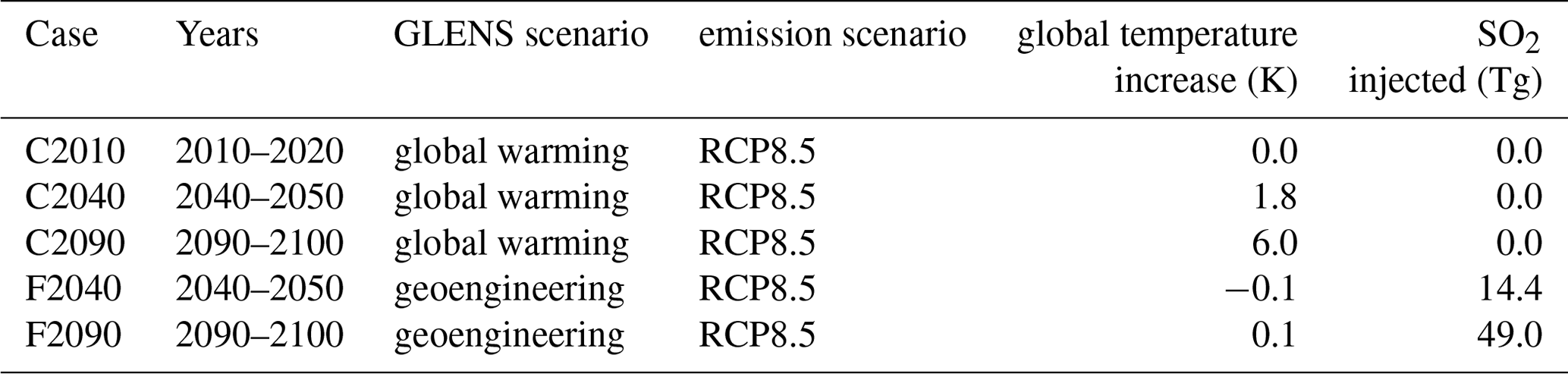
In total five cases are analysed which are determined through the GLENS scenario and the decade. The case C2010 describes conditions in the early 21st century (2010–2020) based on the GLENS global warming scenario. The conditions for the middle (2040–2050) and the end (2090–2100) of the 21st century following the global warming scenario are referred to as cases C2040 and C2090, respectively. The cases of the geoengineering scenario are named F2040 and F2090 for the middle and the end of the 21st century, respectively (“F” stands for the “Feedback” mechanism of the SO2 injections). An overview of the considered cases is given in Table 1 together with the global mean temperature increase reached in that case compared to the conditions of the years 2010–2020 and the injected amount of SO2.
Table 1Overview of the cases analysed in this study. In addition to the years considered, the underlying emission scenario in the GLENS simulation, the global temperature increase (referred to 2010–2020) and the SO2 amount injected by that time period are given for each case.
GLENS results are selected for a latitude range of 30.6–49.5∘ N and a longitude range of 72.25–124.75∘ W (grey area in Fig. 1a) because for this area the reliability of the GLENS C2010 results could be analysed in comparison with aircraft measurements of the SEAC4RS (Studies of Emissions and Atmospheric Composition, Clouds and Climate Coupling by Regional Surveys) and START08 (Stratosphere–Troposphere Analyses of Regional Transport 2008) campaigns. Since the ozone loss process focused on in this study is expected to occur most likely in summer, only the months June, July and August are considered. As shown in Fig. 1b the tropopause altitude varies depending on latitude and the considered case. Since the tropopause altitude varies significantly above central North America, the latitude range is divided into four bins (30–35, 35–40, 40–44 and 44–49∘ N), but in this study the focus is on subtropical latitude band (30–35∘ N) with a more likely subtropical character of the chemical composition and the extratropical latitude band (44–49∘ N) representing the chemical composition of the extratropics around the tropopause.
This study focuses on the mixing layer between tropospheric and stratospheric air located in the lowermost stratosphere above central North America (blue illustrated in Fig. 1a). Without mixing between tropospheric and stratospheric air, correlations of trace gases mainly released in the troposphere (e.g. CO) and mainly produced in the stratosphere (e.g. O3) form an “L shape” (Pan et al., 2004; Vogel et al., 2011) consisting of a tropospheric and a stratospheric branch. A mixing layer between tropospheric and stratospheric air masses additionally generates mixing lines in the tracer–tracer space resulting in “cutting off” the corner of the L shape (e.g. Hoor et al., 2002; Pan et al., 2004; Vogel et al., 2011). The mixing layer in midlatitudes is located close the thermal tropopause, with a significant part in the lowermost stratosphere. Air masses within the mixing layer are characterized by relatively high H2O from the troposphere compared to typically low stratospheric H2O amounts and by O3 and Cly higher than usually found in the upper troposphere from mixing with stratospheric air. Furthermore, the temperatures are low due to the location close to the thermal troposphere. Hence, the lowermost-stratospheric mixing layer shows conditions for which heterogeneous chlorine activation most likely occurs and is therefore the focus of this study.
Since the tropopause altitude and thus the altitude range of the mixing layer varies for different latitudes and future scenarios, the selected altitude range for air masses in the lowermost-stratospheric mixing layer is determined so that it may vary in the considered cases. The lower boundary of the data selected is chosen to be the thermal tropopause calculated according to the WMO definition within GLENS for each time step by the model. The upper boundary is determined by a mixing ratio of 35 ppbv of the artificial E90 tracer. This is a passive tropospheric tracer in WACCM globally released with a lifetime of 90 days, a mixing ratio of ∼90 ppbv at the tropopause and a strong decrease in the lowermost stratosphere (Abalos et al., 2017). Since the E90 tracer is emitted continuously throughout the GLENS simulations, it is independent of possible changes in the emission rates of other tropospheric trace gases and therefore a good marker of the fraction of tropospheric air in the considered air mass.
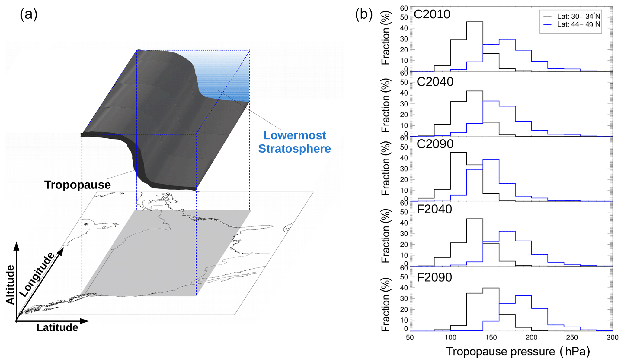
Figure 1Schematic overview of the selected data region over North America (a). The position of the tropopause over central North America in summer is illustrated in black, and the mixing layer is directly located above the tropopause in the lowermost stratosphere (blue). Panel (b) presents the tropopause pressure released from GLENS in this region depending on the latitude range and all considered cases (see Table 1.)
2.2 CLaMS simulations
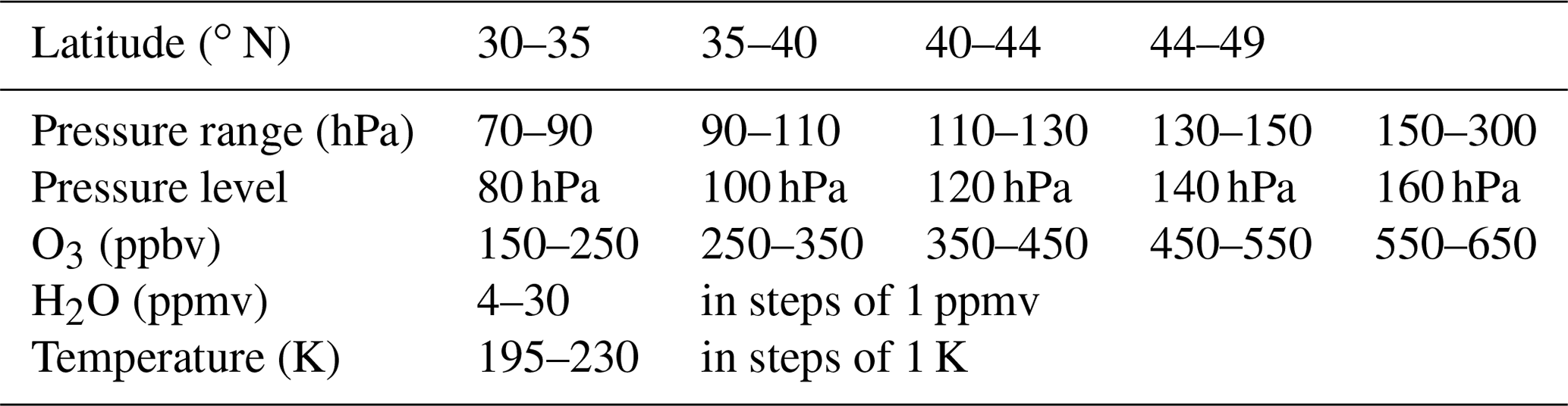
Box-model simulations with CLaMS (e.g. McKenna et al., 2002b, a) are performed to determine chlorine activation thresholds. CLaMS simulations are further initialized based on GLENS results. Therefore, considered GLENS results are divided into different latitude regions, pressure levels and ozone mixing ratios as shown in Table 2. Any combination of latitude, pressure and ozone range is referred to as a data group. The pressure levels are chosen based on the vertical levels used in GLENS. The GLENS results are separated into different ozone ranges because higher ozone mixing ratios are correlated with higher Cly mixing ratios, which promote the likelihood of heterogeneous chlorine activation occurring and its impact on ozone (Robrecht et al., 2019). Furthermore, based on the ozone mixing ratio considered air masses can be divided into those with a chemical composition of air masses typical of the troposphere (low ozone) and those with a chemical composition more typical of the stratosphere (high ozone).
Stratospheric chemistry is simulated along artificial 10-day trajectories, which are designed to calculate the chlorine activation threshold for each data group. Therefore, the trajectories are located at a specific point in the stratosphere determined as 102.5∘ W (middle longitude over the considered longitude range) and the middle pressure and latitude of the specific data group (e.g. 32.5∘ N for the latitude range 30–35∘ N and 80 hPa for the pressure range of 70–90 hPa). As chemical initialization for the CLaMS box model, the median mixing ratio is taken of each trace gas from GLENS in a data group. For each of the five cases (see Table 1) and each data group (Table 2), chemical simulations are conducted assuming constant H2O varying from 4–30 ppmv in steps of 1 ppmv and a constant temperature varying from 195–230 K in 1 K steps resulting in a total of 455 000 box-model simulations. Hereafter, instead of pressure ranges a pressure level as given in Table 2 is used in the text.
Heterogeneous chemistry is only considered here to take place on liquid particles to ensure a comparability to the study of Anderson et al. (2012). Further, only a very low fraction of GLENS data points shows conditions cold enough for the formation of ice particles. As initialization for liquid particles, the particle number density and the gas phase equivalent of H2SO4 is needed, taken from monthly GLENS data as the median of a data group.
Table 2Overview of the latitude, pressure, ozone, H2O and temperature ranges, for which CLaMS simulations are conducted. Each combination of latitude, pressure and ozone range is summarized in a data group resulting in 100 different data groups. For a better overview in this paper, pressure levels are used to describe the pressure ranges (e.g. 80 hPa level for the pressure range 70–90 hPa).
Calculation of the chlorine activation thresholds
The chlorine activation threshold for each data group defines the conditions that allow chlorine-catalysed ozone destruction. Hence, the fraction of GLENS air masses showing these conditions corresponds to the likelihood that ozone destruction occurs as a result of heterogeneous chlorine activation in the North American lowermost stratosphere.
Chlorine activation thresholds are calculated for each data group. Therefore, the H2O and temperature conditions causing chlorine activation within a simulation are identified. Chlorine activation is assumed to have occurred if ClOx contributes 10 % of Cly within the first 5 days of a CLaMS simulation. For each H2O value, the maximum temperature at which chlorine activation occurs is determined to be the temperature threshold for heterogeneous chlorine activation. The array of this temperature threshold depends on a specific H2O mixing ratio, which defines the chlorine activation threshold for the considered latitude, pressure and ozone range.
The selected GLENS results are used as a data set representing the conditions and chemical composition in the mixing layer in the North American lowermost stratosphere in summer for all considered cases for future and today's conditions.

Figure 2Tracer–tracer correlations for the results of case C2010 in a latitude range from 30–35∘ N (a) and SEAC4RS measurements (b) consist of a stratospheric branch (black) and of the mixing layer between stratospheric and tropospheric air masses (red). The mixing layer is determined to be located above the tropopause and showing more than 35 ppbv E90 in case C2010 and more than 31 ppbv CO in SEAC4RS measurements.
3.1 Comparing the GLENS mixing layer today with measurements
The reliability of the selected GLENS mixing layer of the C2010 case is analysed by comparing the mixing layer in case C2010 for the latitude range 30–35∘ N with the mixing layer derived from SEAC4RS ER2 aircraft measurements in August and September 2013. The SEAC4RS campaign was based in Houston (Texas) and one aim was to investigate the impact of deep convective clouds on the H2O content in the lowermost stratosphere (Toon et al., 2016). Hence, SEAC4RS measurements represent moist and cold conditions enhancing the likelihood of heterogeneous chlorine activation occurring. Here, SEAC4RS trace gas measurements are used for CO (Harvard University Picarro cavity ring-down spectrometer (HUPCRS); Werner et al., 2017), O3 (National Oceanic and Atmospheric Administration (NOAA) unmannsed aircraft system O3 instrument; Gao et al., 2012) and H2O (Harvard Lyman-α photo fragment fluorescence hygrometer (HWV); Weinstock et al., 2009). Since GLENS is performed with a global model, the GLENS data cover a broader range in space (regarding altitude and area) than SEAC4RS aircraft measurements, which were locally taken up to an altitude of 20 km. Hence, GLENS and SEAC4RS air masses have a different spatial distribution in the lowermost stratosphere above North America.
The mixing layer between stratospheric and tropospheric air masses in the SEAC4RS measurements is assumed to consist of measurements above the tropopause with a CO mixing ratio of more than 31 ppbv. This CO boundary is selected to allow an O3 range similar to that of the GLENS mixing layer (up to ∼750 ppbv) and agrees with observations in the study by Pan et al. (2004), where mixed air masses between troposphere and stratosphere were described to hold usually more than ∼30 ppbv CO. In Fig. 2, the mixing layer of case C2010 (a) and the SEAC4RS mixing layer (b) are marked in red, while the stratospheric branch is shown in black. Air in the GLENS mixing layer is separated from tropospheric air by being located above the thermal tropopause and from stratospheric air by holding more than 35 ppbv of the E90 tracer. In the mixing layer deduced from SEAC4RS measurements, considered air masses lay above the tropopause as well and are separated here from the stratospheric branch by holding a CO mixing ratio of more then 31 ppbv.
Figure 3a and b show the relative distribution of occurrence frequency of data points in the mixing layer of case C2010 in the temperature–H2O (a, c) and ozone–H2O (b, d) correlation hereafter referred to as relative frequency distribution. For the relative frequency distribution in the temperature–H2O correlation, the number of data points in the mixing layer of case C2010 in all temperature and H2O bins of the size of 1 K × 1 ppmv H2O (Fig. 3a, c) are calculated considering the whole H2O and temperature range given in Table 2. For the relative frequency distribution in the ozone–H2O correlation (Fig. 3b, d), the number of data points in all ozone and H2O bins of the size 10 ppbv O3 × 1 ppmv H2O are calculated. The number of data points of each temperature–H2O (O3–H2O) bin is normalized by the total number of data points found in the mixing layer of case C2010. These fractions are colour-coded in Fig. 3. The relative frequency distribution of data points in the mixing layer derived from SEAC4RS measurements in the same way is shown in Fig. 3c and d.
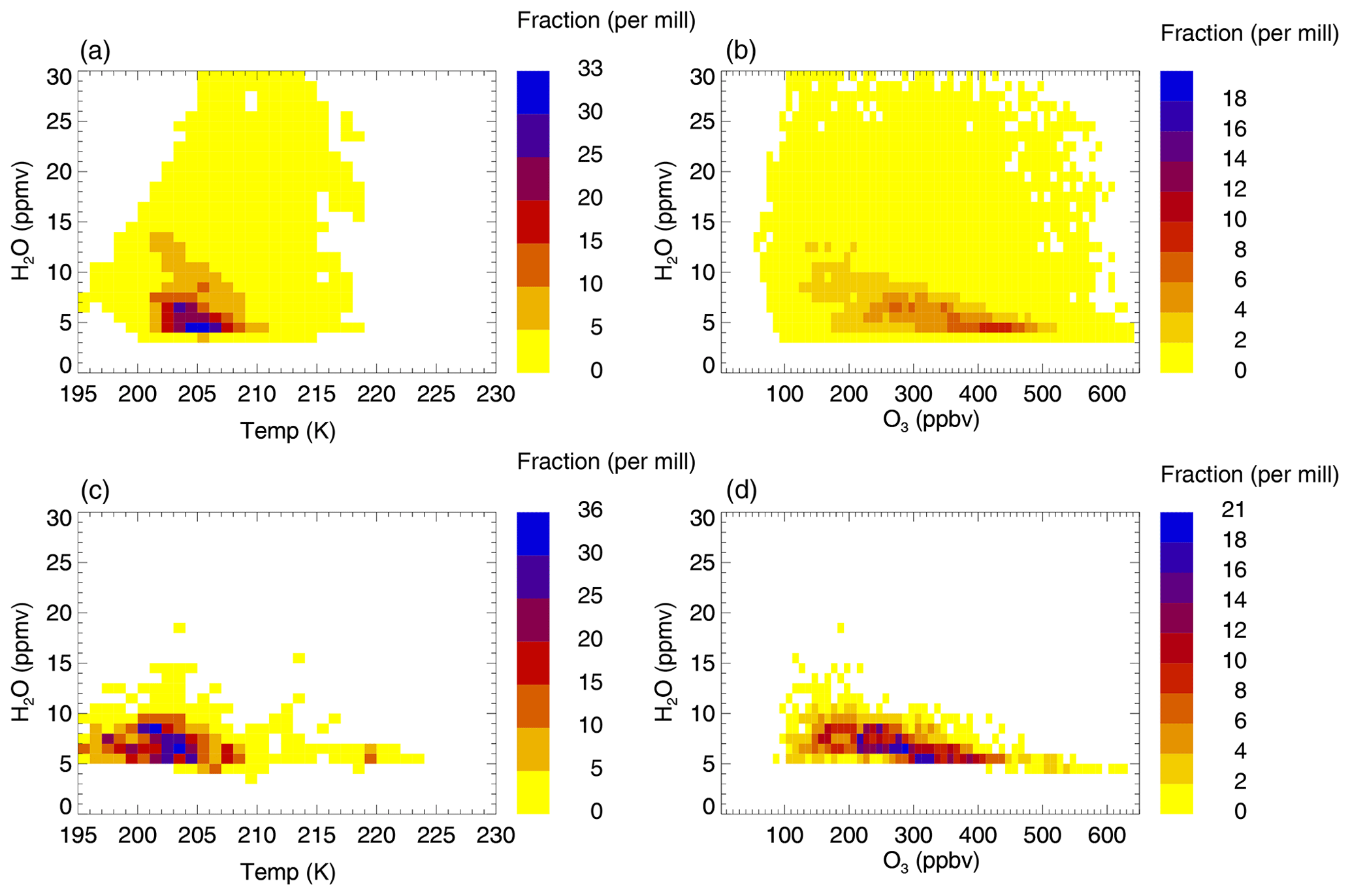
Figure 3Comparison of the relative distribution of the occurrence frequency of data points in the GLENS mixing layer of case C2010 between stratospheric and tropospheric air masses (a, b) with measurements of the SEAC4RS aircraft campaign (c, d). Panels (a) and (c) show the relative frequency distribution regarding H2O and temperature conditions and panels (b) and (d) regarding H2O and ozone mixing ratios. The relative frequency distribution is derived by calculating the number of data points found in a specific temperature and H2O bin (1 K × 1 ppmv H2O; a, c) or ozone and H2O bin (10 ppbv O3× 1 ppmv H2O; b, d) considering all H2O and temperature (ozone) ranges given in Table 2. The number of data points of each temperature–H2O (O3–H2O) bin is normalized by the total number of data points. The colour scheme marks these fractions.
Comparing the SEAC4RS mixing layer with that of case C2010 yields a similar relative frequency distribution regarding temperature and H2O conditions. Above 5 ppmv H2O, the maximum fraction of C2010 and SEAC4RS data resides in the same H2O and temperature range of 201–207 K and 5–8 ppmv H2O (Fig. 3a, c). However, SEAC4RS data show a higher fraction at lower temperatures of 197–200 K and a higher fraction of data in case C2010 has lower H2O mixing ratios than 5 ppmv. Furthermore, C2010 data spread over a broader H2O range.
The SEAC4RS mixing layer and the mixing layer in case C2010 show a similar distribution regarding the H2O–O3 correlation (Fig. 3b, d). A significant fraction of all data corresponds to an ozone range of 200–350 ppbv, but in the C2010 data a higher fraction holds low H2O mixing ratios with an ozone mixing ratio of 400–450 ppbv.
In addition to SEAC4RS measurements, data in the GLENS mixing layer of case C2010 are compared with measurements sampled during the Stratosphere–Troposphere Analyses of Regional Transport (START08) campaign (Pan et al., 2010), which covers a larger latitude range over central North America than the SEAC4RS measurements. The START08 campaign was designed to characterize the transport pathways in the extratropical tropopause region using the U.S. National Science Foundation (NSF) Gulfstream V (GV) research aircraft. START08 measurements show a good overall agreement with GLENS results in case C2010, in spite of the fact that a higher fraction of air masses sampled during START08 has temperatures higher than 215 K caused by the maximum flight height of the GV of ∼14.5 km (for more information see Appendix A).
In general, data points from the modelled case C2010 representing the mixing layer have a good overall agreement with data points in the mixing layer deduced from aircraft measurements above North America. Measurements during SEAC4RS sampled convective injections of H2O into the stratosphere (Toon et al., 2016; Smith et al., 2017; Herman et al., 2017) and thus provide unusually cold and moist conditions for the lowermost stratosphere, which are lower than the temperatures in the simulated C2010 case (∼195–209 K mainly prevailing in SEAC4RS instead of ∼201–209 K in case C2010). To consider the impact of this temperature bias on ozone further simulations are preformed (see Sect. 4.5) assuming temperatures to be 2 and 5 K lower than found in GLENS.
3.2 Change in the chemical composition of the mixing layer
The chemical composition of the mixing layer changes in the GLENS future scenarios. In Fig. 4, the E90–O3 correlation is shown for all considered cases (see Table 1). In the global warming future scenario (C2040, C2090), the O3 mixing ratio increases during the 21st century, but the ozone mixing ratio in the geoengineering scenario (F2040, F2090) remains in a similar range of ∼200–600 ppbv as in case C2010. The correlation between ozone and the artificial tropospheric tracer E90 for C2010 (grey), shown in Fig. 4, agrees well with the F2040 case (red) and the F2090 case (blue). For cases with global warming, the ozone mixing ratio is significantly higher in case C2040 (yellow) and C2090 (green) especially for low E90 concentrations. The enhancement of ozone in the mixing layer could be caused by changes in atmospheric transport or chemistry. Global warming is expected to increase upper-stratospheric ozone and accelerate the BDC. In the considered latitude range, this leads to more ozone transported downwards into the lowermost stratosphere from high altitudes (Iglesias-Suarez et al., 2016).
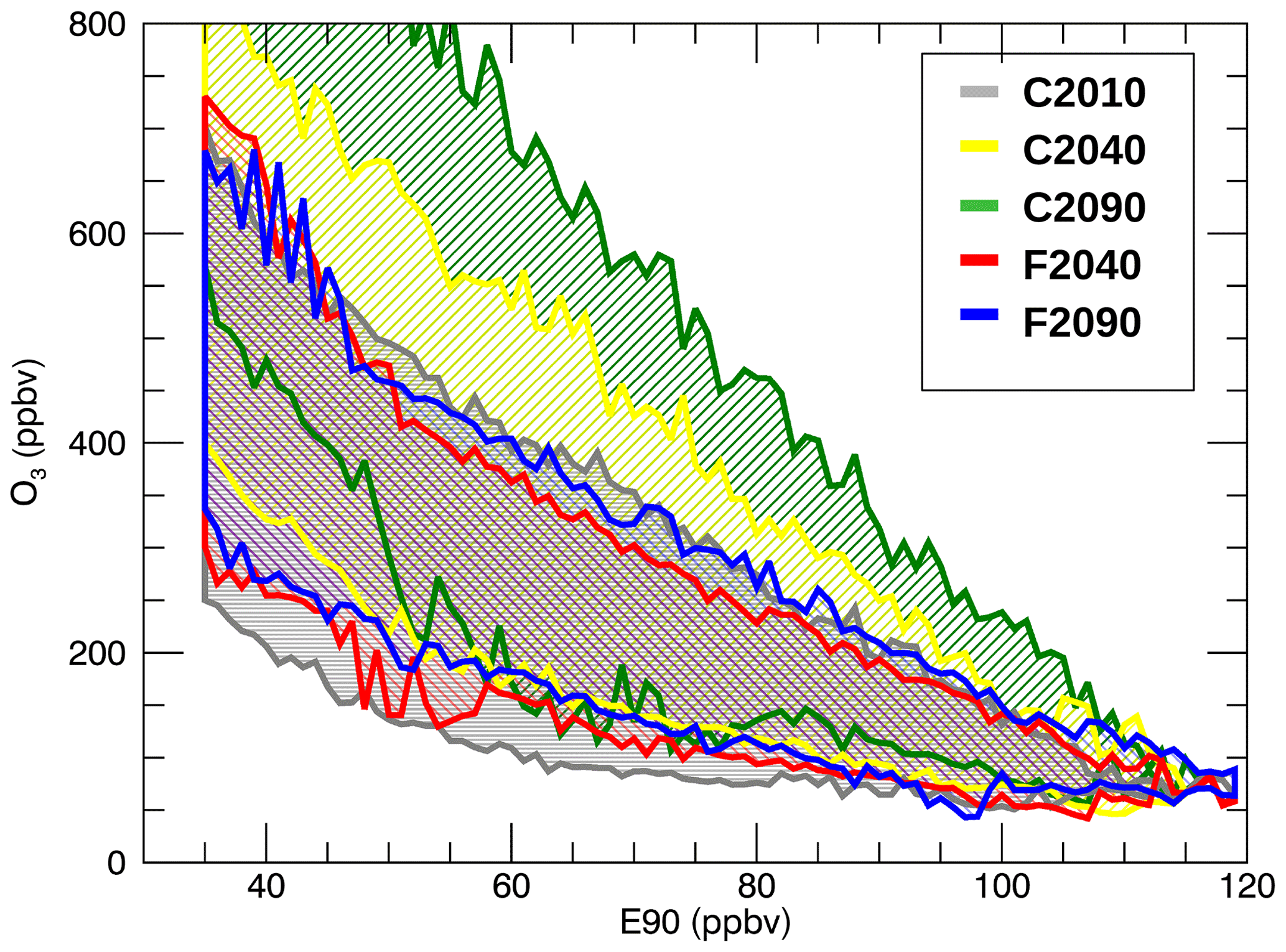
Figure 4O3–E90 correlation in the GLENS mixing layer for today (C2010) and the future scenarios considering both global warming (C2040, C2090) and additional geoengineering (F2040, F2090). An overview of the presented cases is given in Table 1.
Besides changes in transport, ozone in the midlatitude mixing layer could be affected by changes in chemistry (e.g. through chlorine activation). The conditions causing heterogeneous chlorine activation are determined first of all by temperature and H2O mixing ratios. Furthermore, Cly and NOy mixing ratios affect the threshold between conditions, which may or may not lead to chlorine activation. The distribution of temperatures and several trace gas mixing ratios within the GLENS mixing layer for all cases considered is shown in Fig. 5 for the subtropical (30–35∘ N) and the extratropical (44–49∘ N) latitude band over central North America.
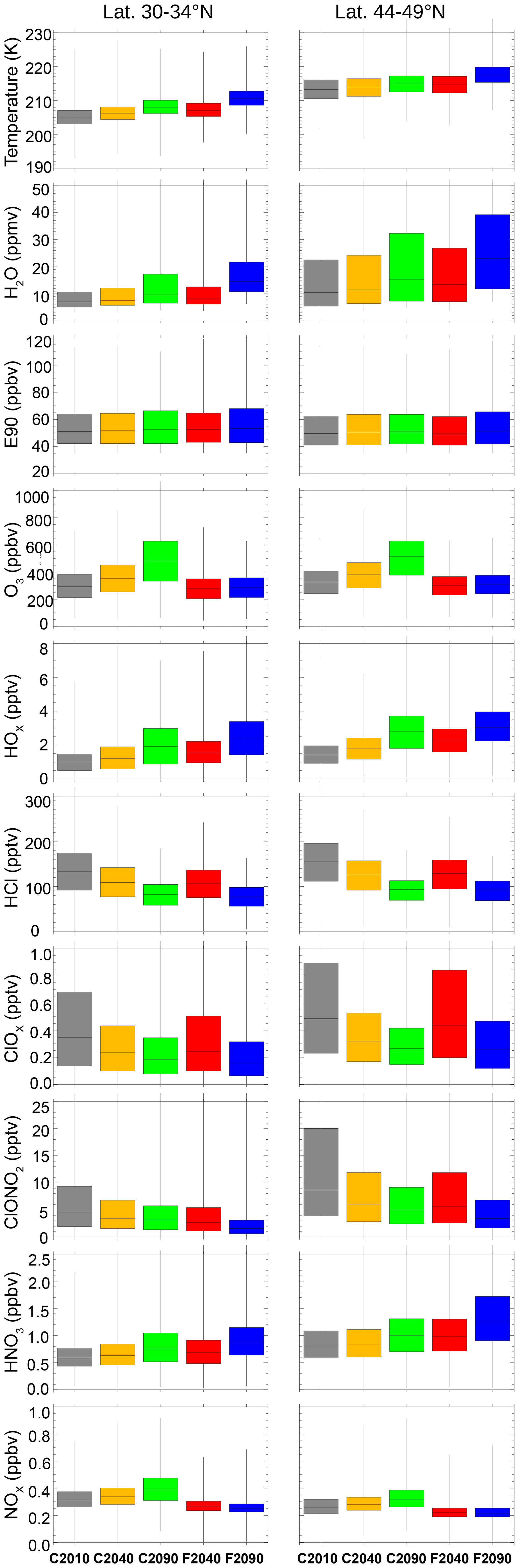
Figure 5Distribution of temperatures and several trace gas mixing ratios in the GLENS mixing layer for case C2010 and future scenarios considering both global warming (C2040, C2090) and sulfate geoengineering (F2040, F2090) (see Table 1). The frequency distribution is illustrated as box plots, where the upper and lower quartile (75 % and 25 %) of the data set is marked by the upper and lower end of the box. The median of the temperature or mixing ratio values within the mixing layer is illustrated by the horizontal line in the box. Ends of vertical lines mark the minimum and the maximum value of the considered data.
In all future scenarios, temperatures and H2O mixing ratios increase (Fig. 5). In the subtropical latitude band, the median temperature increases by ∼3 K from today (case C2010) to the end of the 21st century assuming a global warming scenario (C2090) and by ∼5.5 K when applying geoengineering (case F2090). In the extratropical latitude band, the temperature is higher and shows a similar increasing trend. H2O mixing ratios are higher in the extratropical latitude band than in the subtropical band and spread over a broader range. In both latitude ranges and future scenarios the H2O content increases until the end of the 21st century driven by increasing temperatures of the tropical tropopause layer. An increase in H2O enhances HOx mixing ratios (Fig. 5) and thus accelerates ozone destruction in the HOx cycle.
The HCl and ClOx mixing ratios decrease in the GLENS simulations for both future scenarios due to the implementation of boundary conditions in WACCM according to the Montreal Protocol and its amendments and adjustments. However, the median ClOx mixing ratio is higher by ∼8 (30–34∘ N)–22 % (44–49∘ N) in the F2040 case than in the C2040 case. This could be due to a reduced NOx mixing ratio in the F2040 case. In both future scenarios, the HNO3 mixing ratio increases until the year 2100 (Fig. 5). For global warming, the NOx mixing ratio increases as well. It decreases in the geoengineering scenario because HNO3 formation is accelerated through heterogeneous reactions favoured by a higher aerosol abundance and increasing temperatures enhancing the ratio. Less NOx causes less ClOx to be bound in ClONO2, thus resulting in more gas phase ClOx in the geoengineering scenario. Additionally, the occurrence of heterogeneous chlorine activation could yield an enhancement of ClOx in the geoengineering scenario due to an enhanced aerosol abundance.
The changes in chemistry may affect the future ozone abundance in the lowermost stratosphere. The median ozone mixing ratio increases by 60 %–67 % until the year 2100 in the global warming scenario but remains at today's level in the geoengineering scenario (Fig. 5). The partitioning between active radicals (ClOx, NOx) and reservoir species (HCl, HNO3) differs between the global warming (C2040, C2090) and the geoengineering (F2040, F2090) cases resulting in a different chemical impact on ozone. The likelihood of the occurrence of ozone loss caused by heterogeneous chlorine activation may differ as well in the future scenarios because the heterogeneous chlorine activation is stronger for low temperatures and enhanced H2O mixing values. The likelihood of heterogeneous chlorine activation occurring and its impact on the ozone chemistry are analysed below in the subsequent section.
The H2O and temperature range in which heterogeneous chlorine activation occurs, is determined by calculating chlorine activation thresholds for the specific chemical composition using the CLaMS model. For each case (Table 1), the fraction of all air masses in the GLENS mixing layer between the troposphere and the stratosphere with conditions leading to chlorine activation accounts for the likelihood that chlorine activation occurs. The chlorine activation threshold is determined based on the composition of GLENS air masses in the mixing layer between tropospheric and stratospheric air (see Sect. 3). Chlorine activation thresholds are calculated for all cases (see Table 1) with CLaMS (see Sect. 2.2) for four latitude ranges from 30–49∘ N, five pressure ranges between 70 and 300 hPa and five different ozone ranges from 150–650 ppbv (see Table 2). Ozone values lower than 150 ppbv are not considered here because only a minor fraction of air parcels shows less than 150 ppbv ozone. Furthermore, a critical ozone amount has to be exceeded for chlorine activation to occur (von Hobe et al., 2011) because a higher ozone mixing ratio causes a higher ratio and thus more ClONO2 is formed. This is important for heterogeneous chlorine activation in Reaction (R1) to occur.
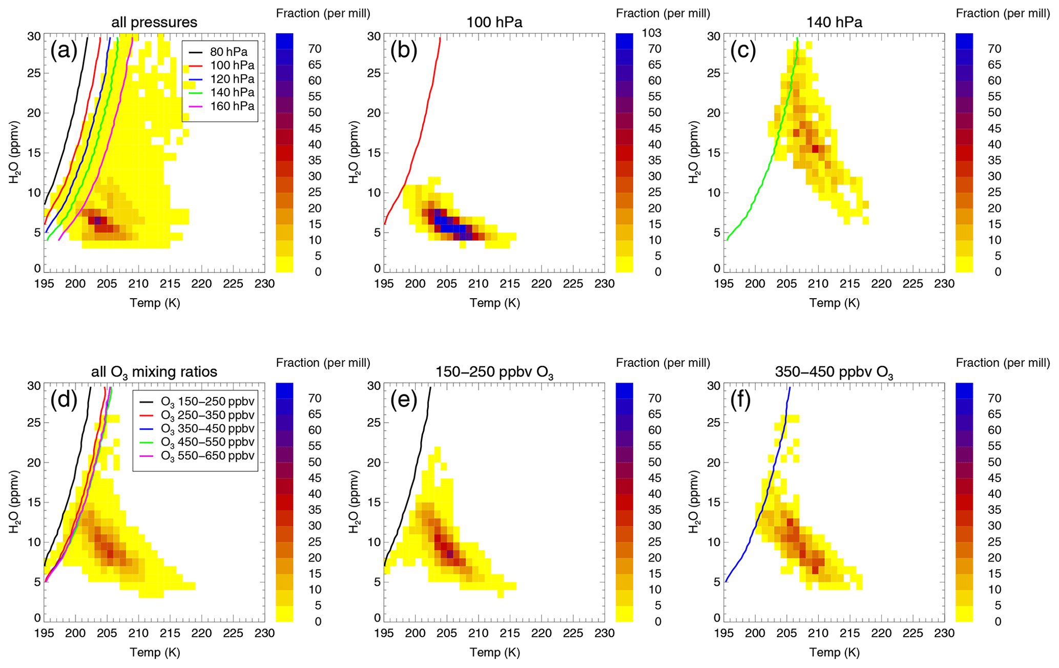
Figure 6H2O–temperature relative frequency distributions and chlorine activation thresholds of different data groups (see Table 2) for the C2010 case and a latitude range of 30–35∘ N. The H2O–temperature relative frequency distribution is illustrated as a colour scheme. The colour marks the fraction of the considered data corresponding to an H2O and temperature bin (1 ppmv H2O × 1 K). The H2O- and temperature-dependent chlorine activation thresholds are marked as a line. Panels (a)–(c) are related to data groups with an ozone mixing ratio of 350–450 ppbv: all data in the considered latitude and ozone range (30–35∘ N, 350–450 ppbv O3) (a); the data group defined by a latitude of 30–35∘ N, an ozone mixing ratio of 350–450 ppbv O3 and the 100 hPa pressure level (b); and the data group defined by a pressure level of 140 hPa and the same latitude and ozone range (c). Panels (d)–(f) are related to data groups with a pressure level of 120 hPa: all data in the considered latitude and pressure level (30–35∘ N, 120 hPa) (d); the data group defined by a latitude of 30–35∘ N, a pressure level of 120 hPa and an ozone mixing ratio of 150–250 ppbv O3 (e); and the data group defined by an ozone mixing ratio of 350–450 ppbv and the same latitude and pressure level (f).
4.1 Analysis of chlorine activation thresholds
Both the chlorine activation threshold and the H2O–temperature relative frequency distribution vary depending on the assumed pressure and ozone level and thus for different data groups. An example for the impact of the pressure and ozone range on the H2O–temperature relative frequency distribution and the chlorine activation threshold is shown in Fig. 6 for the mixing layer of case C2010 in the latitude range of 30–35∘ N.
The H2O–temperature relative frequency distribution is shown (Fig. 6a–c) for an ozone range of 350–450 ppbv. The H2O- and temperature-dependent chlorine activation thresholds are marked as a line for different pressure levels (see Table 2). In Fig. 6a, chlorine activation thresholds are plotted for all pressure levels in the considered latitude and ozone range (30–35∘ N, 350–450 ppbv O3).
At higher pressure levels (lower altitudes), the chlorine activation threshold is shifted allowing chlorine activation to occur at higher temperatures (Fig. 6a). This shift is due to an increasing liquid particle formation as well as more ClONO2 absorbed by an aerosol particle at higher pressures. The heterogeneous chlorine activation rate of Reaction (R1) is determined by the ClONO2 uptake into the aerosol particle (Shi et al., 2001). Air masses lying on the left side of the chlorine activation threshold show chlorine activation. The relative frequency distribution shown in Fig. 6 a is related to all air masses with 350–450 ppbv ozone in a latitude range of 30–35∘ N. Some data points cross various activation thresholds. However, only data points crossing the chlorine activation threshold and in addition corresponding to the pressure level of the activation threshold will yield activated chlorine. As an example, the chlorine activation thresholds at the 100 and 140 hPa level are plotted together with the GLENS relative frequency distribution corresponding to the same data group (Fig. 6b, c). Air masses in the 100 hPa level (Fig. 6b) are colder and dryer than those at 140 hPa (Fig. 6c). Hence, at the 100 hPa level no chlorine will be activated (there are no data corresponding to an H2O–temperature bin on the left side of the threshold line) and chlorine activation occurs for the 140 hPa level only for data points with a high H2O mixing ratio.
In Fig. 6d–f, the H2O—temperature relative frequency distribution and the chlorine activation thresholds are presented for a pressure level of 120 hPa. The impact of the ozone mixing ratios on the chlorine activation threshold is illustrated. Figure 6d shows the GLENS H2O–temperature relative frequency distribution and the chlorine activation thresholds for all data groups corresponding to the selected latitude range and pressure level (30–35∘ N, 120 hPa). Higher ozone mixing ratios are related to higher Cly amounts. Hence, an increase in ozone shifts the chlorine activation threshold to higher temperatures (Fig. 6d). However, considering the relative frequency distribution of specific data groups with different ozone levels, data points with more ozone are warmer than those with less ozone (Fig. 6e, f).
In the future scenarios, the H2O–temperature relative frequency distribution as well as the chlorine activation thresholds vary. In Fig. 7 the H2O–temperature relative frequency distribution is shown for the cases C2010, C2090 and F2090. The relative frequency distributions are shown for the subtropical latitude band (30–35∘ N, Fig. 7a–c) and for the extratropical latitude band (44–49∘ N, Fig. 7d–f). For each case shown, additionally, a selection of chlorine activation thresholds is shown. These are related to different ozone and pressure levels and give a range of uncertainty for the H2O and temperature ranges causing chlorine activation.
In agreement with the changes in the conditions in the mixing layer described in Sect. 3, the future H2O–temperature relative frequency distributions (C2090 in Fig. 7b, F2090 in Fig. 7c) are both moister and warmer than the conditions today (C2010, Fig. 7a). However, the geoengineering case F2090 exhibits data significantly warmer and moister than reached in the global warming case C2090. In the extratropical latitude band (Fig. 7d–f), temperatures are generally higher than in the subtropical latitude range.
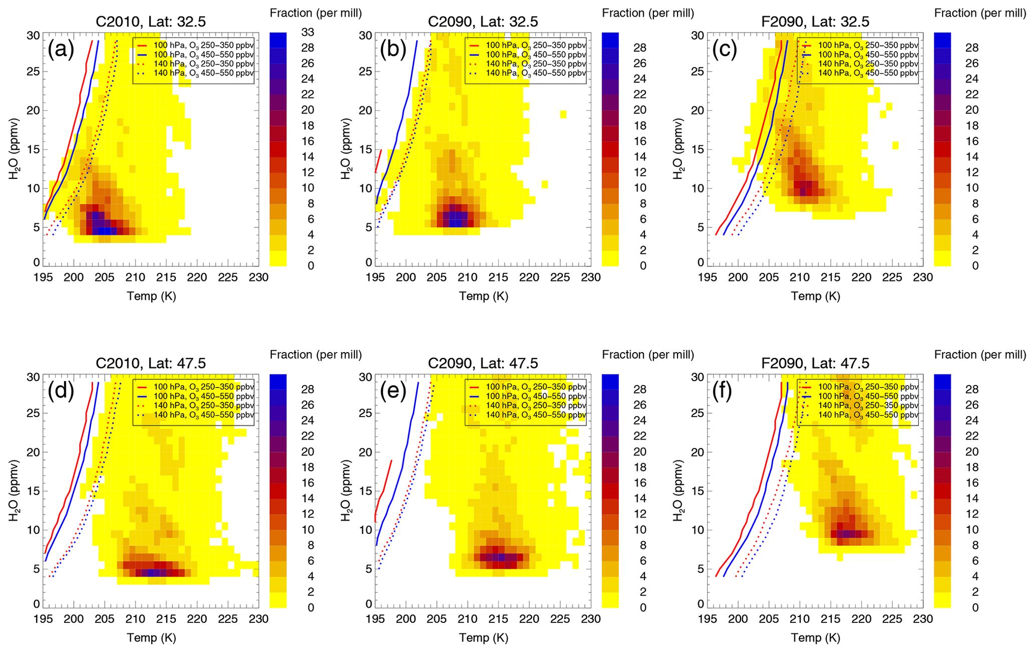
Figure 7H2O–temperature relative frequency distributions and examples for chlorine activation thresholds for the cases C2010 (a, d) and the future scenarios at the end of the 21st century assuming global warming (C2090, b, e) and additional geoengineering (F2090, c, f) for the subtropical latitude band (30–35∘ N, a–c) and the extratropical band (44–49∘ N, d–f). The colour marks the fraction of the considered data corresponding to an H2O and temperature bin (1 ppmv H2O × 1 K). The H2O- and temperature-dependent chlorine activation threshold is marked as a line for exemplarily chosen data groups specified in the legend of each panel.
Considering the chlorine activation thresholds in Fig. 7, the largest fraction of air masses corresponds to temperatures greater than the chlorine activation thresholds. The chlorine activation thresholds for the C2090 case are shifted to lower temperatures compared to case C2010 because of the lower chlorine abundance (a higher Cly mixing ratio promotes heterogeneous chlorine activation; Robrecht et al., 2019). In contrast, in the geoengineering scenario F2090 chlorine activation can occur at higher temperatures than today in spite of the lower chlorine amount. This is caused by the higher aerosol loading due to the applied geoengineering.
In each case, the H2O and temperature bins marked by the chlorine activation thresholds to potentially cause heterogeneous chlorine activation are in good agreement for both latitude ranges presented. Since the temperatures of the mixing layer are higher in the extratropical latitude band, the fraction of air masses crossing the chlorine activation threshold and thus causing chlorine activation is lower in that latitude range (44–49∘ N) than in the subtropical latitude band (30–35∘ N).
There are some chlorine activation thresholds that cannot be reported when the H2O mixing ratio exceeds a certain value (e.g. Fig. 7e, 100 hPa, 250–350 ppbv O3). At such high H2O mixing ratios, HCl is absorbed strongly into the aerosol particles, reducing gas phase Cly, and thus less ClONO2 may be formed. Since chlorine is activated in Reaction (R1) (HCl+ClONO2), less ClONO2 leads to a lower chlorine activation rate. HCl uptake into supercooled water particles was also found to occur after volcanic eruptions resulting in an “HCl scavenging”, which may protect the ozone layer (Tabazadeh and Turco, 1993). In our study the effect of HCl uptake is negligible if the Cly mixing ratio is high enough. But if the Cly mixing ratio is low (e.g. in a low ozone range in the years 2090–2099), reducing gas phase Cly by absorbing HCl into the aerosol results in no activation of chlorine. Hence, there is no chlorine activation for these conditions.
Summarizing, the H2O- and temperature-dependent chlorine activation threshold marks an upper boundary of temperatures causing heterogeneous chlorine activation for air masses with a specific H2O mixing ratio. Thus for a given H2O mixing ratio, the maximum temperature at which chlorine activation may occur is determined by the chlorine activation threshold. In this section, we showed that the chlorine activation thresholds and the H2O–temperature relative frequency distribution of the mixing layer in the GLENS simulations depend on the aerosol abundance, pressure and the Cly mixing ratio, which is related to the ozone level. Moist and very cold air masses, which in general are expected to promote heterogeneous chlorine activation, usually correspond to low pressures and low ozone mixing ratios. Hence, the pressure and ozone dependence of chlorine activation results in only few air masses with conditions suitable to activate chlorine. Thus, chlorine activation thresholds have to be compared with air masses in GLENS corresponding to the same data group regarding pressure, ozone and latitude range as the calculated chlorine activation threshold to deduce the likelihood that chlorine activation occurs.
4.2 Likelihood of ozone destruction today and in the future
The likelihood of chlorine activation occurring is quantified here as the fraction of air masses in the GLENS mixing layer between tropospheric and stratospheric air, which are cold and moist enough to cause heterogeneous chlorine activation. Comparing GLENS air masses with chlorine activation thresholds for each case, the number of air masses is counted showing lower temperatures than determined as the threshold temperature for chlorine activation. The fraction of this amount in all air masses within the mixing layer of the considered case yields the likelihood of heterogeneous chlorine activation occurring. Here, we assume that chlorine activation always results in ozone destruction processes known from polar late winter and early spring (e.g. Molina and Molina, 1987; McElroy et al., 1986; Crutzen et al., 1992; Solomon, 1999). Hence, the likelihood of chlorine activation occurring is the same as the likelihood of chlorine-catalysed ozone destruction.
In Fig. 8a, the likelihood of chlorine activation occurring is presented considering air masses in the entire latitude range (30–49∘ N). Each panel corresponds to a considered case (C2010, C2040, C2090, F2040 and F2090; see Table 1). The likelihood of chlorine activation occurring is marked by the height of a bar: for single pressure levels and named “all” for all air masses within the mixing layer. In the C2010 case, the overall likelihood of chlorine activation occurring is 1.0 % in the entire latitude and pressure level (Fig. 8a, left panel, left bar). However, chlorine activation occurs most likely in the pressure level of 140 hPa. A fraction of 3.5 % of all air masses in the 140 hPa level causes heterogeneous chlorine activation in the C2010 case. As described in Sect. 4.1, higher pressures increase the aerosol formation and uptake of ClONO2 into the liquid aerosol particles, which determines if chlorine activation through Reaction (R1) (Shi et al., 2001) occurs. Thus, the chlorine activation threshold is shifted to higher temperatures at higher pressures. However, the likelihood of chlorine activation is lower at 160 hPa than at 140 hPa (Fig. 8) because air masses corresponding to higher pressure levels are warmer than those with a lower pressure (example shown in Fig. 6b, c). Air masses in the 160 hPa level are significantly warmer than air masses in the 140 hPa level. Hence, although the chlorine activation threshold is shifted to higher temperatures for the 160 hPa pressure level, most air masses corresponding to this high pressure are to warm for heterogeneous chlorine activation and chlorine activation occurs most likely in the 140 hPa level.
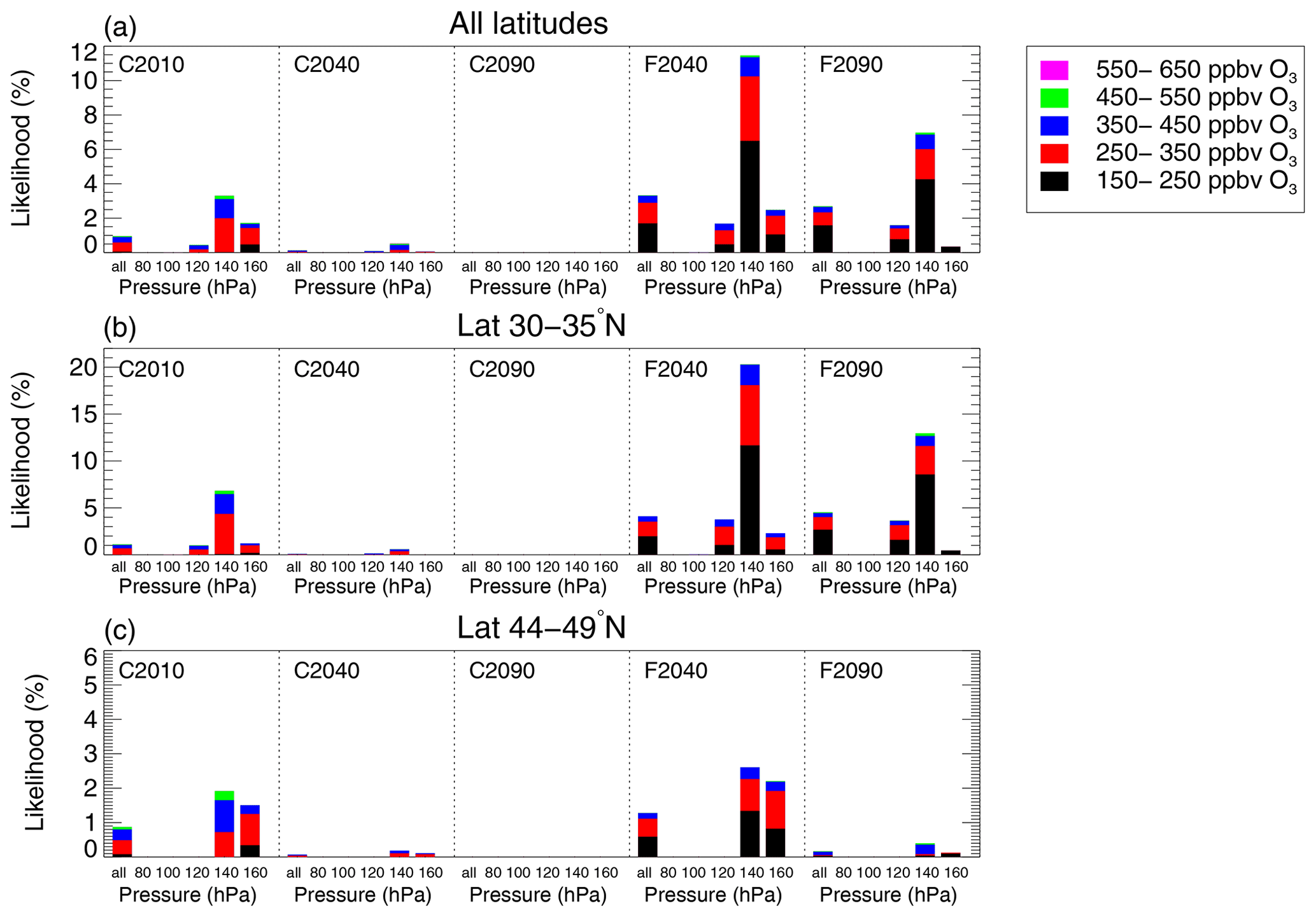
Figure 8Likelihood of heterogeneous chlorine activation occurring in different latitude regions in the mixing layer for all considered cases of today and the future scenarios (see Table 1). The entire latitude range above central North America (30–49∘ N) is considered in (a), only the subtropical latitude band (30–35∘ N) is considered in (b), and only the extratropical latitude band (44–49∘ N) is considered in (c). Different panels correspond to different cases given at the top of each panel. The height of the bars marks the likelihood of a specific pressure level given under that bar. The pressure range corresponding to a given pressure level is given in Table 2. The denotation “all” refers to the whole pressure range of the mixing layer. Colours indicate the likelihood of chlorine activation occurring for air masses with different ozone ranges. Note the different y axes for the three rows.
The contribution of different ozone levels in the air masses, which show chlorine activation, is additionally marked by the colour scheme in Fig. 8. In case C2010, chlorine activation mainly occurs in air masses with an ozone mixing ratio of 250–350 ppbv (Fig. 8a).
Focussing on the future scenarios, the likelihood of chlorine activation occurring is very low in the global warming cases C2040 and C2090 (Fig. 8a). In contrast, the likelihood in the geoengineering cases F2040 and F2090 is higher than for today (case C2010). Chlorine activation occurs most likely at the middle of the 21st century in case F2040, where 3.3 % of all air masses in the mixing layer would cause chlorine activation. In the 140 hPa level, 11.5 % of the air masses cause chlorine activation in case F2040. The likelihood of chlorine activation occurring is slightly lower at the end of the 21st century due to the decrease in Cly implemented in GLENS. In case F2090, 2.7 % of all air masses in the mixing layer cause chlorine activation.
The likelihood of chlorine activation in different latitude ranges is illustrated in Fig. 8b (latitude range of 30–35∘ N) and c (latitude range of 44–49∘ N). In general, chlorine activation occurs more likely in the subtropical latitude band (30–35∘ N) than in extratropical (44–49∘ N) latitudes because of the different temperature range and chemical composition around the tropopause in the tropics and extratropics (note the different y scales for different latitude ranges in Fig. 8). In case C2010, 1.1 % of all air masses in the subtropical latitude band (30–35∘ N) and 0.9 % in the extratropical latitude band (44–49∘ N) causes chlorine activation. In both latitude ranges, the likelihood of chlorine activation is negligible in the future cases C2040 and C2090. In contrast, the likelihood increases in the geoengineering scenario. In case F2040, 4.1 % of all air masses in the subtropical latitude band of the mixing layer cause chlorine activation. In the same latitude range, the likelihood of chlorine activation occurring is higher in case F2090 (4.5 %), in spite of the implemented decrease in stratospheric Cly. The likelihood increases between case F2040 and F2090 because in case F2090 a higher fraction of air masses has a pressure corresponding to the 120 hPa and the 140 hPa level than in case F2040 (not shown). In contrast, in the extratropical latitudes (44–49∘ N), the likelihood of chlorine activation occurring is higher in case F2040 (1.3 %) than in case F2090 (0.2 %) caused by the decrease in stratospheric Cly and the warming of the mixing layer. In this latitude range, the likelihood of chlorine activation occurring is generally lower than in the subtropical latitude band because the temperatures in the simulated mixing layer are higher (see Fig. 5).
Focussing on the ozone mixing ratio of air masses in which chlorine activation occurs in the simulated mixing layer, the colour scheme in Fig. 8 indicates that chlorine activation occurs more likely in air masses with low ozone mixing ratios than in air masses with high ozone mixing ratios. This is in agreement with the dependence of the H2O–temperature relative frequency distribution in the mixing layer on the ozone mixing ratio discussed in Sect. 4.1 (shown as an example in Fig. 6). Air masses with higher ozone mixing ratios are warmer than those with less ozone and thus cause less likely heterogeneous chlorine activation.
In summary, the occurrence of chlorine activation and the resulting catalytic ozone loss processes similar to those known from polar regions are unlikely based on the comparison of GLENS results with chlorine activation thresholds for all cases considered. However, chlorine activation occurs more likely in the future scenario assuming geoengineering than in today's case C2010. In the future scenario assuming global warming, the likelihood of chlorine activation occurring is negligible. Furthermore, chlorine activation is more likely at lower latitudes than at higher latitudes. Since air masses causing chlorine activation usually show low ozone mixing ratios, the ozone amount affected by chlorine-catalysed ozone destruction is expected to be low. How relevant the activation of chlorine is for the ozone chemistry in the midlatitude lowermost stratosphere is analysed in the next section.
4.3 Impact of heterogeneous chlorine activation on ozone in the lowermost stratosphere
How much ozone in the mixing layer above central North America is affected by the heterogeneous chlorine activation process is analysed here by considering the ozone changes in the CLaMS simulations together with the relative frequency distribution in the temperature–H2O correlation in GLENS. Briefly, ozone changes in CLaMS correspond to an upper boundary for the conditions assumed during the simulation and the relative frequency distribution comprises the fraction of data points with the same H2O and temperature conditions as assumed during the simulation. Hence, from combining the ozone change in CLaMS simulations with the relative frequency distribution in both scenarios simulated in GLENS (global warming and geoengineering), the impact of this ozone loss process on ozone in the mixing layer can be determined.
In more detail, CLaMS simulations are conducted for all data groups and any combination of temperature and H2O bins. The difference between initial and final ozone within each 10-day simulation yields for each data group (determined by a latitude, pressure and ozone range; see Table 2) the chemical ozone change corresponding to a particular H2O and temperature bin (1 K × 1 ppmv H2O in a range of 195–230 K and 4–30 ppmv H2O). Since no mixing is allowed in the box-model runs, the conditions that yield chlorine activation are not disturbed within 10 days. In the lowermost stratosphere, the duration of conservation for conditions causing chlorine activation is not yet known. However, mixing of cold and moist air from the troposphere uplifted to above the tropopause (e.g. through convective overshooting) with dry and warmer stratospheric air will reduce the H2O content of the moist air parcel. Since the occurrence of chlorine activation depends on both the temperature and the H2O mixing ratio of the air parcel, a decrease in H2O can stop chemical chlorine activation. Hence, assuming the maintenance of chlorine activation for 10 consecutive days without a perturbation by mixing here yields an upper boundary for the impact of heterogeneous chlorine activation on ozone in the midlatitude lowermost stratosphere.
The chemical ozone change between the initial and final ozone of a 10-day box-model simulation is multiplied with the number of GLENS air masses corresponding to the same data group and H2O and temperature bin. In this way, the total chemical ozone change in the midlatitude mixing layer is estimated. The total initial ozone is calculated by multiplying the median ozone amount of each data group with the number of GLENS air masses corresponding to that data group. The ratio of the total ozone change from the start to the end of the 10-day CLaMS simulation and the total initial ozone yields the relative ozone change.
The relative ozone change in the mixing layer determined from the difference between final and initial ozone in the 10-day CLaMS box-model simulations for each considered case is illustrated as black bars in Fig. 9a. In case C2010, chemical ozone formation dominates the ozone chemistry in the mixing layer and causes an increase in ozone of 2.3 %. In the future global warming scenario, ozone would increase by around 2.5 % within 10 consecutive days of unperturbed chemistry in case C2040 and by 3 % in case C2090. In the geoengineering scenario, the relative chemical ozone formation is lower than following a global warming. However, the ozone change increases from +2.3 % in the F2040 case to +2.6 % in the F2090 case. The increasing ozone formation in the future may be related to the reduction in ODSs implemented in both GLENS scenarios. The lower chemical ozone increase in the mixing layer for the geoengineering scenario is based on an increase in ozone destruction processes. Ozone destruction catalysed by HOx radicals is more likely in the geoengineering scenario because of the higher HOx mixing ratio (Fig. 5). Furthermore heterogeneous chlorine activation could yield ozone destruction.

Figure 9Relative chemical ozone change in the mixing layer determined from the difference between initial and final ozone in the 10-day CLaMS box-model simulations (no mixing between air masses) in all considered cases (see Table 1). The relative ozone change is shown (a) considering the entire latitude region above central North America (black bars) as well as only considering the subtropical (30–35∘ N, red bars) or extratropical (44-49∘ N, blue bars) latitude region. Further, the ozone change from air masses in which chlorine activation can occur normalized by the total initial ozone from all air masses in the simulated mixing layer is shown (b).
The relative ozone change caused by heterogeneous chlorine activation is shown in Fig. 9b for all cases. For calculating the relative ozone change caused by heterogeneous chlorine activation, ozone changes corresponding to air masses which cause chlorine activation are multiplied with the number of these air masses in the GLENS mixing layer. This ozone change from air masses in which chlorine activation can occur is normalized with the total initial ozone of all air masses in the GLENS mixing layer. Black bars correspond to air masses in the entire latitude region above central North America. In case C2010, 0.1 % of ozone in the mixing layer would be destroyed within 10 consecutive days caused by heterogeneous chlorine activation. In the global warming scenarios, chlorine activation causes less ozone destruction in the mixing layer. Heterogeneous chlorine activation has the strongest impact on ozone in the mixing layer of the F2040 case. In this case, 0.3 % of ozone in the mixing layer would be destroyed if the chemical conditions yielding chlorine activation are maintained for 10 days. In comparison, for the conditions in case F2090 0.1 % of ozone in the mixing layer would be destroyed.
In Fig. 9, additionally the relative ozone change calculated based on 10-day CLaMS box-model simulations is illustrated with respect to the latitude ranges 30–35∘ N (red bars) and 44–49∘ N (blue bars). Comparing the relative ozone change in different latitude regions, in the subtropical latitude band more ozone is formed (Fig. 9a). For example in case C2010, ozone increases by 3.4 % in the subtropical latitude band (30–35∘ N) and by 1.2 % at 44–49∘ N. However, in the subtropical latitude band heterogeneous chlorine activation affects ozone more (Fig. 9b). Heterogeneous chlorine activation causes the strongest ozone destruction in the mixing layer for the geoengineering case F2040 with an ozone destruction of 0.4 % in 10 consecutive days in 30–35∘ N. In contrast, in case C2040 less than 0.1 % would be destroyed in the same latitude range.
Since in the subtropical latitude range (30–35∘ N) the effect of heterogeneous chlorine activation on ozone is the highest, the relative ozone change in that latitude range is shown in more detail with respect to single pressure levels in Fig. 10. In general, ozone formation processes dominate at low pressures, causing a net chemical ozone increase (Fig. 10a). At higher pressure levels, the net ozone formation is lower. Furthermore, the occurrence of heterogeneous chlorine activation is more likely at higher pressure levels. In the F2040 case where heterogeneous chlorine activation has the strongest impact on ozone chemistry in the mixing layer, up to 2.1 % of total initial ozone in the pressure level of 140 hPa are destroyed in air masses with conditions allowing heterogeneous chlorine activation (Fig. 10b). When both the ozone destruction in air masses allowing chlorine activation and ozone formation in the other air masses in the 140 hPa level are considered the net ozone change at this pressure level accounts for −0.7 % (Fig. 10a).
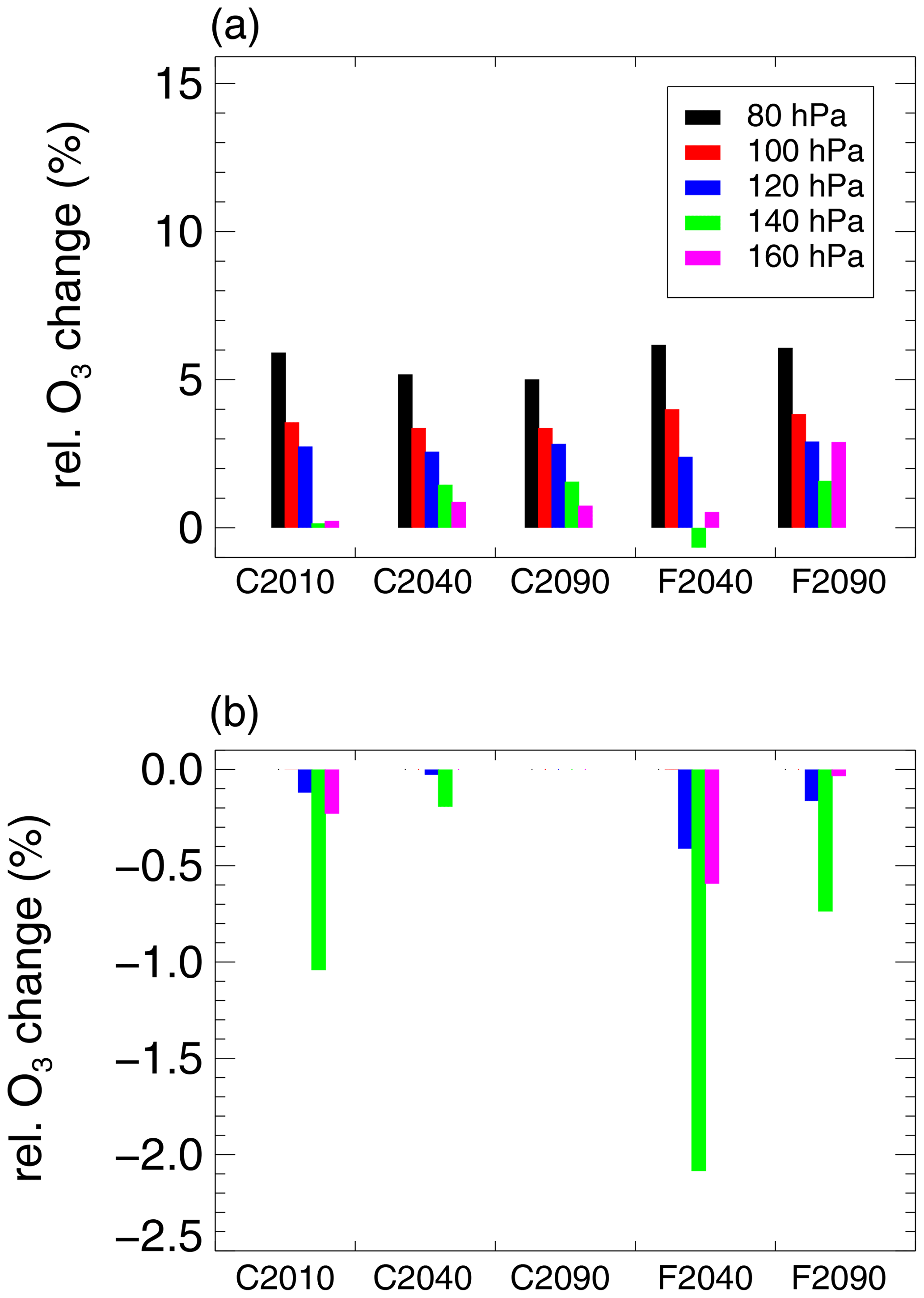
Figure 10Relative chemical ozone change in the subtropical latitude band (30–35∘ N) in the mixing layer determined from the difference between initial and final ozone for the 10-day CLaMS box-model simulations in the considered cases (see Table 1). The overall ozone change (a) within single pressure levels between 70 and 300 hPa (see Table 2) is shown as well as the ozone change from air masses in which chlorine activation can occur normalized by the total initial ozone from all air masses in the GLENS mixing layer (b).
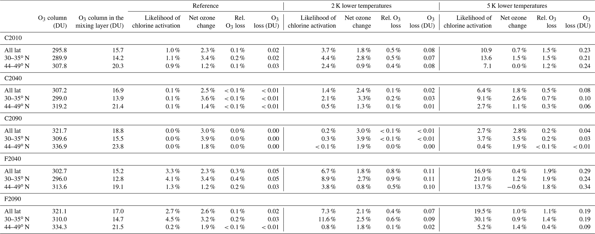
The likelihood of chlorine activation occurring in the midlatitude mixing layer just above the tropopause, the relative ozone change caused by heterogeneous chlorine activation and the net chemical ozone change in the mixing layer are summarized in Table 3 considering the entire latitude range (30–49∘ N) as well as the subtropical (30–35∘ N) and the extratropical (44–49∘ N) latitude band. The results calculated here are referred to as “reference”.
In general, the impact of heterogeneous chlorine activation causing chlorine-catalysed ozone destruction on ozone in the midlatitude lowermost stratosphere is low. Combining the occurrence of conditions in the scenarios simulated in GLENS with the chemical ozone change determined through CLaMS box-model simulations, in all cases a net chemical ozone formation will occur above central North America. However, chlorine activation may affect ozone in the mixing layer. In the geoengineering scenario in case F2040 chlorine activation has the highest impact on ozone in comparison to the other cases and can cause an ozone reduction of up to 0.38 %.
Table 3Overview of the likelihood of chlorine activation occurring in the midlatitude mixing layer above the tropopause, its impact on ozone in the mixing layer and the relevance for ozone column. Further the net chemical ozone change in the mixing layer is specified. Three latitude ranges are considered here: 30–49∘ N, only the subtropical latitude band in 30–35∘ N and only the extratropical latitude band in 44–49∘ N. The considered cases today (C2010) and in the future scenarios assuming global warming (C2040, C2090) and additional geoengineering (F2040, F2090) are further described in Table 1. The reference refers to GLENS results for the mixing layer. In the assumption with 2 K (5 K) lower temperatures, temperatures of GLENS air masses are reduced by 2 K (5 K) to infer uncertainties in the simulated temperatures. The chemical ozone changes here are determined based on 10-day box-model simulations neglecting mixing between neighbouring air masses. Thus conditions causing chlorine activation are assumed here to be maintained for 10 consecutive days without perturbations.
4.4 Relevance of heterogeneous chlorine activation in the mixing layer for the midlatitude ozone column
In the previous section, the variability of ozone reduction caused by heterogeneous chlorine activation in the midlatitude mixing layer between tropospheric and stratospheric air was determined for different cases. Based on this relative ozone change in the mixing layer, the impact of heterogeneous chlorine activation in the midlatitude lowermost stratosphere on column ozone is deduced.
For all of the GLENS cases today and in the future (see Table 1), first the ozone profile is determined by averaging over the ozone mixing ratio within each GLENS vertical level. Both the entire latitude region above central North America and the specific latitude regions (30–35 and 44–49∘ N) are considered. Subsequently, the column ozone is calculated from the ozone profile. In Table 3 the total column ozone is shown as well as the ozone column in the mixing layer.
The ozone column in the mixing layer is assumed to correspond to the ozone column in a pressure range from 70–300 hPa. Even though the mixing layer comprises pressures between 70 and 300 hPa, not all air masses within this pressure range are necessarily part of the mixing layer because only air parcels above the thermal tropopause and with more than 31 ppbv CO are assumed to form the stratospheric mixing layer between tropospheric and stratospheric air. Hence, for determining the ozone column in the mixing layer, not only air masses in the mixing layer but also all further air masses between 70 and 300 hPa are considered. Since the composition of air parcels in the mixing layer consists of lowermost-stratospheric air mixed with tropospheric air, the ozone mixing ratio in these air parcels is somewhat smaller than the mixing ratio in air masses with the same pressure range and stratospheric character. Hence, the ozone column deduced from all air parcels in a pressure range from 70–300 hPa is expected to be somewhat larger than it would be considering only air parcels in the mixing layer. Thus in Table 3, the ozone column in the mixing layer might be overestimated.
In Sect. 4.3 the relative ozone destruction in the mixing layer caused by heterogeneous chlorine activation was determined and is given in Table 3. From the relative ozone loss and the ozone column in the mixing layer, the ozone loss caused by heterogeneous chlorine activation in Dobson units (DU) can be calculated.
The relative ozone loss in the mixing layer caused by heterogeneous chlorine activation is low. Thus, the maximum total ozone loss given in Table 3 is negligible compared with the total ozone column. Even in case F2040, where the chlorine activation causes most ozone destruction in the mixing layer, the total ozone loss accounts for no more than 0.05 DU. This is less than 0.1 % of the total ozone column.
4.5 Likelihood of heterogeneous chlorine activation and its impact on ozone for low temperatures
As analysed in Sect. 3.1, the temperatures in the mixing layer above the tropopause simulated in GLENS may be higher than the real atmospheric temperatures in this region. Therefore, a sensitivity study is performed assuming a reduction in GLENS temperatures of −2 K and of −5 K to explore the impact of uncertainties in the temperatures calculated in GLENS. However, the focus of this sensitivity assumption is only on the temperature reduction without considering a potential ice formation at very low temperatures. The likelihood of the occurrence of heterogeneous chlorine activation assuming lower temperatures and its impact on ozone in the lowermost stratosphere is presented in Fig. 11.
The likelihood that chlorine activation occurs would increase significantly assuming lower temperatures (Fig. 11a, b). For case C2010, chlorine activation would occur with a likelihood of 3.7 % assuming 2 K lower temperatures and of 10.9 % assuming 5 K lower temperatures than in the GLENS simulation (assuming GLENS temperatures, the likelihood accounts for 1.0 %). In the global warming cases C2040 and C2090 the likelihood increases likewise assuming lower temperatures. In case C2040, assuming temperatures of 2 K less yields a likelihood of 1.4 %, and assuming 5 K less it yields a likelihood of 6.4 % (instead of 0.1 % assuming GLENS temperatures). In case C2090, for −5 K, the likelihood accounts for 2.7 %. Applying geoengineering would cause the highest likelihood of chlorine activation occurring. Assuming 2 K lower temperatures than the GLENS simulations, in case F2040 6.7 % (16.9 % for −5 K) and in case F2090 7.4 % (19.5 % for −5 K) of the air masses would yield chlorine activation.
Despite the higher likelihood of chlorine activation in the F2090 case, ozone is more affected in the F2040 case because the ozone values in the range where ozone destruction would occur in the years 2040–2050 are higher than in the years 2090–2100 (not shown). For 2 K lower temperatures, activated chlorine would destroy up to ∼0.8 % of ozone in the lowermost stratosphere in the F2040 case, but only up to 0.4 % in case F2090 (Fig. 11e, f). Assuming 5 K less, 1.9 % (F2040) and 1.1 % (F2090) of ozone in the lowermost stratosphere are destroyed. In the global warming scenario, more ozone would be likewise destroyed due to heterogeneous chlorine activation.
The higher ozone destruction due to chlorine activation for lower temperatures results in a reduced net ozone formation in the mixing layer. For all cases considered (global warming and geoengineering), the relative net ozone change (Fig. 11c, d) is significantly reduced. In case F2040 in the extratropical latitude range, even a net ozone destruction occurs in the mixing layer assuming 5 K less than simulated in GLENS. However, comparing the behaviour in different latitude regions, the impact of heterogeneous chlorine activation on ozone is mostly higher in lower latitudes.
The likelihood of heterogeneous chlorine activation occurring and its impact on ozone in the mixing layer determined in this section is summarized in Table 3 referred to as “2 K” and “5 K” lower temperatures. Assuming less temperatures than those calculated in GLENS increases the likelihood of heterogeneous chlorine activation occurring as well as its impact on lowermost-stratospheric ozone. In all cases, the relative ozone loss in the mixing layer is 2 to 3 times higher assuming 2 K lower temperatures than in the reference and 6 to 10 times higher in the −5 K assumption. Assuming low temperatures, in all cases considered, an upper limit of 0.3 DU from a total ozone column of ∼303 DU in this region (which is ∼0.1 %) has been estimated as the total ozone reduction caused by heterogeneous chlorine activation.
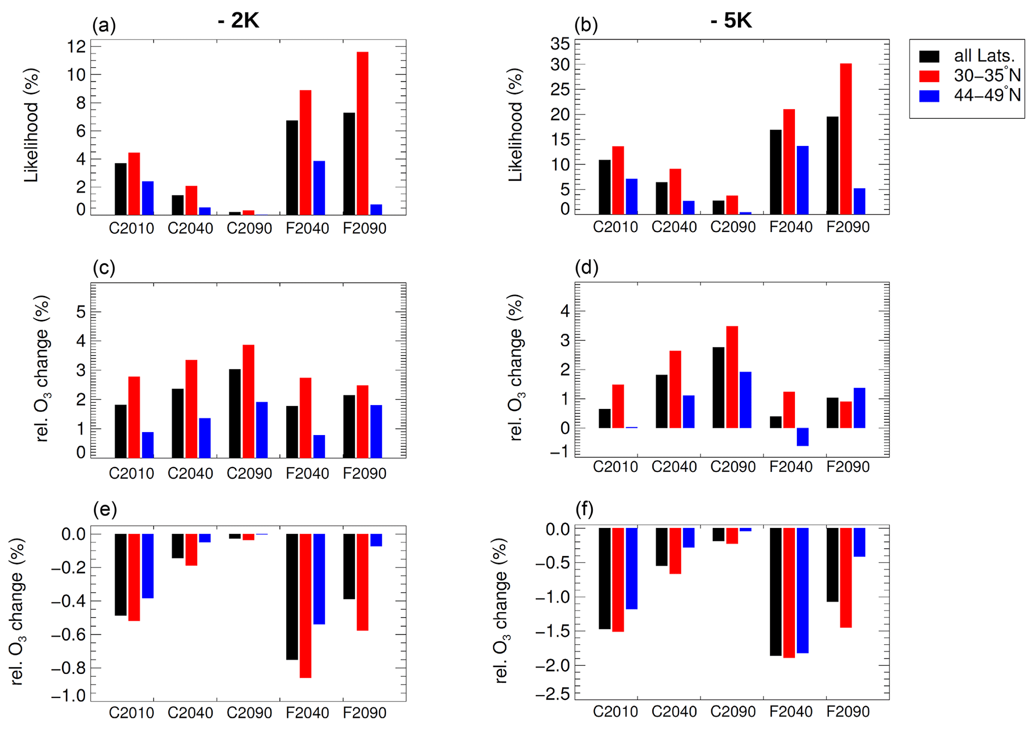
Figure 11Likelihood (a, b) for the occurrence of chlorine activation as well as its impact on ozone in the lowermost stratosphere assuming 2 K (a, c, e) and 5 K (b, d, f) lower temperatures than simulated in GLENS. Further, the chemical ozone change in the mixing layer assuming 10 consecutive days without mixing of air parcels (c, d) and the relative ozone change in the mixing layer caused by heterogeneous chlorine activation (e, f) is shown for the assumption with 2 and 5 K less temperatures. Note that the scale on the y axes differs (see Table 1 for case descriptions).
We analysed the relevance of heterogeneous chlorine activation for the ozone changes in the lowermost stratosphere today and in future assuming both global warming and the application of sulfate geoengineering.
Assuming global warming, median ozone in the mixing layer increases by 60 % in the subtropics (30–35∘ N) and by 67 % in the extratropics (44–49∘ N) by the end of the 21st century (case C2090). In contrast, Ball et al. (2018) reported evidence for a decrease in midlatitude lower-stratospheric ozone between the years 1998 and 2016. This ozone decrease was interpreted as dynamically driven (Chipperfield et al., 2018; Ball et al., 2019) by non-linear effects not yet completely understood and usually not implemented in climate models (Ball et al., 2019). However, this ozone decrease was found to be small with respect to the inter-annual variability. This decrease results in a total ozone reduction of 1.9 DU between the years 1998 and 2018 in the lower stratosphere at 30–50∘ N. In comparison, ozone loss caused by heterogeneous chlorine activation analysed here and potentially occurring in the midlatitude lower stratosphere in summer is found to cause an ozone loss of less than 0.1 DU for present day conditions (case C2010) in the same latitude range.
This reduction in column ozone is determined here from the relative ozone loss in the mixing layer and the contribution of ozone in the mixing layer to total column ozone. In case C2010, air masses in a pressure range between 70 and 300 hPa contribute 4.9 % to the ozone column in a latitude range of 30–35∘ N and 6.6 % in 44–49∘ N. In comparison, Logan (1999) found a contribution of ozone between the thermal tropopause and 100 hPa on the total ozone column in summer of ∼6 % in a latitude of 38∘ N and of ∼17 % in 53∘ N. Thus in case C2010, the mixing layer contributes less to the ozone column than in the study of Logan (1999) deduced from satellite measurements between the years 1980 and 1993. However, if ozone in the mixing layer in case C2010 would contribute as much to column ozone as in the study of Logan (1999), 0.03 DU of ozone would be destroyed for today's conditions at 30–35∘ N and 0.05 DU at 44–49∘ N.
In all cases investigated here, a net chemical ozone formation occurs in the lowermost stratosphere. Ozone is formed there due to high CO and CH4 mixing ratios which result from transport from the troposphere to the lowermost stratosphere. Hence, the oxidation of CO and CH4, which usually forms ozone in the upper troposphere, causes ozone formation in the lowermost stratosphere as well (Lelieveld et al., 1997; Johnston and Kinnison, 1998). However, a potential ozone destruction in the midlatitude lowermost stratosphere due to heterogeneous chlorine activation was discussed in previous studies (e.g. Keim et al., 1996; Anderson et al., 2012, 2017; Anderson and Clapp, 2018; Schwartz et al., 2013; Berthet et al., 2017; Robrecht et al., 2019; Clapp and Anderson, 2019; Schoeberl et al., 2020).
This chlorine-driven ozone loss process could occur today above central North America in relation to stratospheric moistening through convective overshooting events during the North American Summer Monsoon (NAM). However, convection implemented in WACCM does not consider overshooting convection (i.e. convection up to above the local tropopause) and therefore the transport of enhanced H2O into the lower stratosphere by convection is most likely underestimated in the GLENS simulations. Anderson and Clapp (2018) performed a box-model study, where they assume that conditions yielding heterogeneous chlorine activation, as low temperatures and a high H2O mixing ratio of 20 ppmv, are maintained for 14 consecutive days. With this assumption, they simulated a maximal fractional ozone loss of −2.5 % to −67 % (depending on the HCl mixing ratio) for the lower stratosphere between 12 and 18 km. In our study, chlorine activation would reduce ozone in the mixing layer by 0.1 % for today's conditions (case C2010; 0.7 % assuming 5 K lower temperatures).
In comparison, Schwartz et al. (2013) argue that conditions cold and moist enough for chlorine activation are very rare and are usually associated with low HCl and ozone amounts. Schoeberl et al. (2020) found that lowermost-stratospheric H2O is increased during the NAM caused by enhanced convection followed by advection in the monsoon circulation. Simultaneously, the tropopause is uplifted reducing column ozone. However, this correlation between enhanced H2O in the lowermost stratosphere and reduced column ozone is found to be dynamically driven with no evidence of substantial chemical ozone loss caused by chlorine activation.
An enhancement of the stratospheric sulfate abundance, which causes ozone destruction in relation to heterogeneous chlorine activation, was mentioned in previous studies with respect to volcanic eruptions. Keim et al. (1996) combined laboratory measurements and observations and reported a removal layer for ozone caused by heterogeneous chlorine activation in the midlatitudes around the tropopause subsequent to the Mt. Pinatubo eruption. Solomon et al. (1998) accentuated the relevance of heterogeneous chlorine chemistry by calculating a column ozone loss of ∼4 % after the eruption of El Chichón and of ∼10 % after the eruption of Mt. Pinatubo in 40–50∘ N not considering fluctuations of dynamical forcing between different years. However, Solomon et al. (1998) considered the entire ozone column, not only ozone loss in the lowermost stratosphere.
In our study, only air masses that are close to the tropopause are considered. Nevertheless, it is very unlikely that ozone loss caused by heterogeneous chlorine activation occurs at higher altitudes. As shown in Sect. 4.2 the likelihood is highest for a pressure level around 140 hPa because chlorine activation is favoured at high pressures. Furthermore, temperatures increase with altitude reducing the likelihood of chlorine activation occurring. Since the stratospheric Cly concentration decreases because of the Montreal protocol, the impact of heterogeneous chlorine chemistry on ozone in the future is expected to be lower than for volcanic eruption in the past.
Comparing lowermost-stratospheric ozone in the global warming and the geoengineering scenario, the overall ozone mixing ratio at the end of the 21st century is higher in the global warming scenario. There are other processes than heterogeneous chlorine activation which are not investigated here and which would affect stratospheric ozone by applying sulfate geoengineering. For example, an increase in H2O would increase HOx catalysed ozone destruction (Heckendorn et al., 2009), and changes in radiation could affect oxygen and ozone photolysis. Furthermore, increased heterogeneous chemistry could enhance the NOx concentration and gas phase chemistry could change due to higher stratospheric temperatures (Pitari et al., 2014). Since both chemistry and dynamics can affect stratospheric ozone at geoengineering conditions in multiple ways (e.g. Heckendorn et al., 2009; Pitari et al., 2014; Tilmes et al., 2009, 2014; Visioni et al., 2017b), further studies are necessary to assess the impact of geoengineering on stratospheric ozone (e.g. quantifying changes in HOx-induced ozone destruction or investigating the dynamical contribution to the difference in the ozone mixing ratio between the global warming and the geoengineering scenario).
Here, we focus on the potential occurrence of heterogeneous chlorine activation in the mixing layer between stratospheric and tropospheric air above central North America (30.6–49.5∘ N, 72.25–124.75∘ W), which leads to catalytic ozone destruction known from the stratosphere during polar late winter and early spring. The likelihood of chlorine activation occurring and its impact on ozone in the mixing layer today and in future is determined by comparing chlorine activation thresholds with the temperature and water vapour (H2O) distribution in GLENS (Geoengineering Large Ensemble simulations). The chlorine activation thresholds were calculated based on CLaMS box-model simulations considering initial conditions for trace gases and aerosols from GLENS. In GLENS, two future scenarios are simulated with a global climate model from the years 2010–2100 considering both global warming following the RCP8.5 scenario and the additional application of geoengineering through stratospheric sulfate injections beginning in the year 2020 to keep the global mean temperature at the levels from 2020.
The GLENS mixing layer will warm and moisten in both future scenarios with a larger change in the geoengineering scenario (the median temperature is ∼2.5 K higher in the years 2090–2100 with geoengineering than with global warming and the median H2O mixing ratio is ∼6.5 ppmv higher). The ozone mixing ratio increases in the midlatitude mixing layer in GLENS assuming the global warming future scenario but is found to remain at today's level when sulfate geoengineering is applied. These differences may be due to changes in both atmospheric dynamics and chemistry in the lowermost stratosphere. For example, potential chemical effects are an increasing HOx mixing ratio because of a higher H2O mixing ratio or differences in the - or the partitioning driven by changes in the heterogeneous and gas phase chemistry.
GLENS results in the mixing layer are analysed in comparison with SEAC4RS aircraft measurements. Most GLENS results and SEAC4RS measurements in the mixing layer range from 201–207 K and 5–8 ppmv H2O. Thus, the H2O and temperature conditions in GLENS have a good overall agreement with current observations. However, in the SEAC4RS measurements a higher fraction of air parcels with very low temperatures of 197–200 K compared to GLENS results are found. Based on this difference catalytic ozone loss is additionally investigated for 2 and 5 K lower temperatures than in the GLENS results.
A temperature- and H2O-dependent threshold indicates conditions which lead to and which do not lead to heterogeneous chlorine activation. The chlorine activation threshold analysed in this study marks an upper temperature limit for chlorine activation to occur at a given H2O mixing ratio. We showed that the chlorine activation thresholds depend on a variety of conditions. Increasing pressure, sulfate aerosol loading and ozone mixing ratio allow higher temperatures to cause chlorine activation. However, air parcels with higher pressures, sulfate aerosol loadings or ozone mixing ratios are usually warm. Hence, shifting chlorine activation thresholds to higher temperatures (and thus leading to a broader range of conditions allowing chlorine activation) does not necessarily increase the likelihood of chlorine activation occurring because the temperatures of air masses with the pressure and composition leading to these chlorine activation thresholds increase as well.
The likelihood of heterogeneous chlorine activation occurring and its impact on ozone in the mixing layer between tropospheric and stratospheric air masses is determined for several cases, which differ in the future scenario and in the considered years as further described in Table 1. The comparison of chlorine activation thresholds with GLENS results yields a likelihood of chlorine activation occurring of 1.0 % for case C2010 and, assuming geoengineering, of 3.3 % in case F2040 and 2.7 % in case F2090. In contrast, the likelihood is negligible in the global warming scenario (0.1 % in case C2040 and 0.0 % in C2090). Assuming 2 K lower temperatures, the likelihood increases accounting for 3.7 % in case C2010, 6.7 % and 7.3 % in the cases F2040 and F2090, respectively, and 1.4 % and 0.2 % in the cases C2040 and C2090, respectively. Assuming 5 K lower temperatures, the likelihood is higher with 10.9 % in case C2010, 2.7 % in case C2090 (global warming) and 19.5 % in case F2090 (geoengineering). We showed that the likelihood of occurrence is higher at lower latitudes and at higher pressure levels (lower altitudes). However, in air masses in which chlorine activation may occur, usually a low ozone mixing ratio prevails. This fact contributes to the low impact of chlorine activation on ozone in the mixing layer.
The net chemical ozone change in the mixing layer is calculated here by combining the change in the ozone mixing ratio from 10-day CLaMS box-model simulations (final ozone − initial ozone) assuming specific H2O and temperature conditions with the GLENS frequency distribution in the H2O and temperature correlation. Normalizing this net chemical ozone change with the total initial ozone in the mixing layer yields the net relative ozone change, which occurs if chemical processes proceed for 10 days without being perturbed by mixing between air parcels. In addition it should be noted that convection used in WACCM does not consider overshooting convection (i.e. convection up to above the local tropopause) and therefore the transport of enhanced H2O into the lower stratosphere by convection is most likely underestimated in our study. Thus, in today's C2010 case the net relative ozone change in the mixing layer accounts for +2.3 %. Also in the future scenarios, a net chemical ozone formation occurs. In the global warming future scenario, ozone increases within 10 days by ∼2.5 % in case C2040 and by ∼3.0 % in case C2090. In the sulfate geoengineering scenario, the increase is somewhat less with 2.3 % in case F2040 and 2.6 % in case F2090.
However, little ozone is destroyed due to heterogeneous chlorine activation. In case F2040, which is the case with the largest ozone destruction, 0.3 % of ozone in the stratospheric mixing layer is destroyed due to heterogeneous chlorine activation. Ozone destruction is larger in the subtropical latitude range (30–35∘ N). In that latitude range, 0.4 % of ozone would be destroyed in the F2040 case and 0.2 % in 44–49∘ N. Assuming lower temperatures, less ozone would be formed during 10 days without mixing. Additionally the relative ozone destruction in the mixing layer above central North America in case F2040 would increase to 0.8 % assuming 2 K lower temperatures than simulated in GLENS and 1.9 % assuming 5 K lower temperatures.
Finally, the impact of heterogeneous chlorine activation in the mixing layer is estimated. Based on the conditions in GLENS, in all cases less than 0.1 DU of ozone (less than 0.1 % of the ozone column) is destroyed due to heterogeneous chlorine activation in the mixing layer. Assuming 5 K lower temperatures, not more than 0.34 DU of ozone are destroyed for all latitude regions and all cases today and in the future scenarios with global warming as well as with additional sulfate geoengineering. In comparison in the Arctic polar winter in the year 2000, a volcanically clean year, 77±10 DU were destroyed between 110–30 hPa (Vogel et al., 2003), and Tilmes et al. (2008) have shown significantly larger ozone depletion in high polar latitudes with geoengineering.
In summary, we show that heterogeneous chlorine activation affects ozone in the lowermost stratosphere in midlatitudes, but the impacts are very small. Sulfate geoengineering leads to a 2–3 times higher likelihood of the occurrence of chlorine activation. However, in the geoengineering case most likely for chlorine activation, chlorine is activated with a probability of 3.3 % (16.9 % assuming 5 K lower temperatures) in the entire latitude region considered here. In all cases today and in future, less than 0.4 % (1.9 % assuming 5 K lower temperatures) of ozone in the mixing layer are destroyed due to heterogeneous chlorine activation. This leads to a reduction in column ozone of 0.1 DU (0.3 DU if 5 K lower temperatures are assumed), which are 0.1 % of column ozone. Thus according to the results of this study, the relevance of ozone destruction caused by heterogeneous chlorine activation in the midlatitude mixing layer between stratospheric and tropospheric air is negligible with respect to the ozone column and small in the mixing layer even if sulfate geoengineering would be applied.
In addition to measurements of the SEAC4RS campaign, data from the GLENS mixing layer in case C2010 are compared with measurements of the Stratosphere–Troposphere Analyses of Regional Transport (START08) aircraft campaign (Pan et al., 2010). START08 aimed to investigate the stratosphere-to-troposphere transport focussing on stratospheric intrusions into the troposphere and tropospheric intrusions transporting air masses from the upper tropical troposphere to the extratropical lowermost stratosphere. Flights during START08 took place from April–June 2008 and covered the area above central North America (25–65∘ N, 80–120∘ W) up to an altitude of ∼14.3 km (Pan et al., 2010).
In Fig. A1, the GLENS tracer–tracer correlation of the GLENS mixing layer in case C2010 is compared with the mixing layer deduced from START08 measurements. Air masses corresponding to the mixing layer between stratospheric and tropospheric air are assumed to be located above the thermal tropopause estimated based on the temperature–altitude profile during the flight. In addition they are selected to show more than 30 ppbv CO and more than 150 ppbv O3. In contrast to the SEAC4RS mixing layer (Sect. 3.1), the ozone criteria are added to determine the mixing layer from START08 measurements because many data points above the tropopause deduced from temperatures measured during the flight exhibited very low ozone mixing ratios indicating a high fraction of air from the troposphere above the tropopause. This tropospheric air masses crossing the thermal tropopause were aimed to be probed during the START08 campaign.
The comparison of the stratospheric GLENS E90–O3 correlation with the START08 CO–O3 correlation is shown in black in Fig. A1a, b. In contrast to GLENS results, ozone measurements during START08 only reach up to ∼1400 ppbv O3 because of the limitation of the probed altitude by the maximum flight height of ∼14.3 km. However, the mixing layer in GLENS (red) comprises a similar ozone range as the mixing layer deduced from START08 measurements.
In Fig. A1c, d, the H2O–temperature correlation (Fig. A1c) and the H2O–O3 correlation (Fig. A1d) for the entire latitude region considered in this study are shown. Figure A1e and f show the same correlations for the mixing layer deduced from START08 measurements. In both model results and measurements, the H2O mixing ratio exceeds more than 30 ppmv and the ozone mixing ratio ranges mainly between 300 and 500 ppbv. However, GLENS temperatures are somewhat lower than temperatures measured during START08.
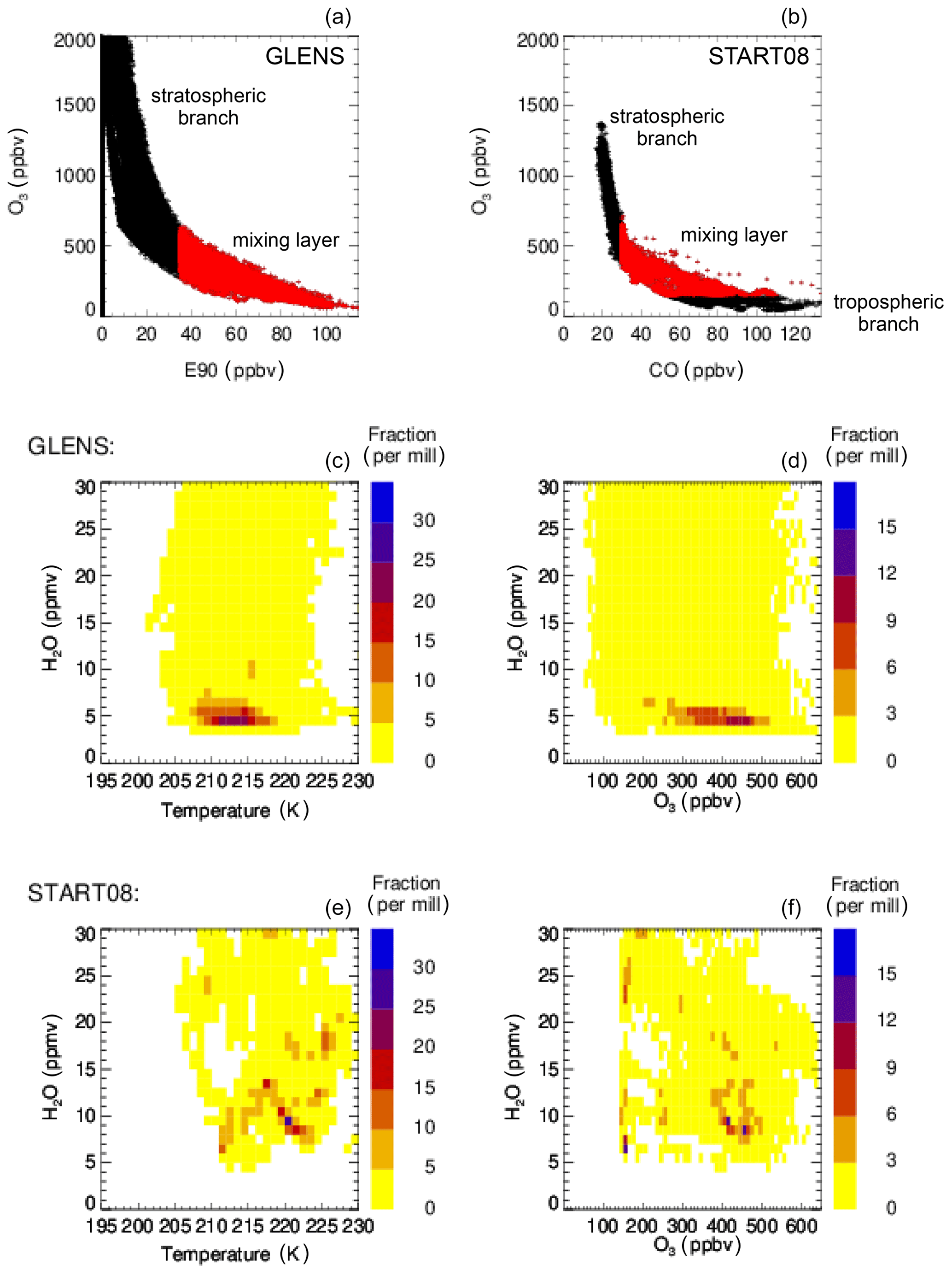
Figure A1Comparison of the GLENS mixing layer between stratospheric and tropospheric air masses of the C2010 case with measurements of the START08 aircraft campaign. Panels (a) and (b) show the E90–O3 correlation of GLENS air masses (a) and the CO–O3 relative frequency distribution of START08 measurements (b) for stratospheric air masses (black) and air masses corresponding to the mixing layer (red). Panels (c) and (d) show the relative frequency distribution in the H2O–temperature (c) and the H2O–O3 (d) correlation of the GLENS mixing layer, and panels (e) and (f) show the distribution of the mixing layer deduced from START08 measurements.
CLaMS is available at the following GitLab server: https://jugit.fz-juelich.de/clams/CLaMS (last access: 14 February 2020, CLaMS, 2020).
Access options for GLENS data are given at https://doi.org/10.5065/D6JH3JXX (Tilmes et al., 2020). The results of CLaMS simulations can be requested from Sabine Robrecht (sa.robrecht@fz-juelich.de). The complete SEAC4RS data are available at https://www-air.larc.nasa.gov/cgi-bin/ArcView/seac4rs (last access: 27 May 2020, NASA, 2020) and options to access START08 data are given at https://data.eol.ucar.edu/master_lists/generated/start08/ (last access: 27 May 2020, NCAR, 2020).
All authors developed the concept of the study. SR conducted CLaMS simulations, analysed GLENS results and wrote the paper with contributions from all authors.
The authors declare that they have no conflict of interest.
We thank the groups of Ru-Shan Gao (NOAA Chemical Sciences Laboratory, Boulder, CO, USA), Jessica Smith (Harvard University, Department Earth and Planetary Science, Cambridge, MA, USA) and Steven Wofsy (Harvard University, Department Earth and Planetary Science, Cambridge, MA, USA) for providing their data measured during the SEAC4RS aircraft campaign. We further thank Dale Hurst (NOAA ESRL Global Monitoring Division, Boulder, CO, USA) and the NCAR Earth Observing Laboratory team (NCAR, Boulder, CO, USA) for providing START08 data. For GLENS, computing resources were provided by the Climate Simulations Laboratory (CISL).
Our activities were funded by the German Science Foundation (Deutsche Forschungsgemeinschaft, DFG) under the DFG project CE-O3 in the context of the Priority Program “Climate Engineering: Risks, Challenges, Opportunities?” (grant nos. SPP 1689 and VO 1276/4-1).
The article processing charges for this open-access publication
were covered by a Research Centre of the Helmholtz Association.
This paper was edited by Farahnaz Khosrawi and reviewed by Daniele Visioni and one anonymous referee.
Abalos, M., Randel, W. J., Kinnison, D. E., and Garcia, R. R.: Using the artificial tracer E90 to examine present and future UTLS tracer transport in WACCM, J. Atmos. Sci., 74, 3383–3403, https://doi.org/10.1175/JAS-D-17-0135.1, 2017. a
Anderson, J. G. and Clapp, C. E.: Coupling free radical catalysis, climate change, and human health, Phys. Chem. Chem. Phys., 20, 10569–10587, https://doi.org/10.1039/C7CP08331A, 2018. a, b
Anderson, J. G., Wilmouth, D. M., Smith, J. B., and Sayres, D. S.: UV dosage levels in summer: Increased risk of ozone loss from convectively injected water vapor, Science, 337, 835–839, https://doi.org/10.1126/science.1222978, 2012. a, b, c, d, e, f, g
Anderson, J. G., Weisenstein, D. K., Bowman, K. P., Homeyer, C. R., Smith, J. B., Wilmouth, D. M., Sayres, D. S., Klobas, J. E., Leroy, S. S., Dykema, J. A., and Wofsy, S. C.: Stratospheric ozone over the United States in summer linked to observations of convection and temperature via chlorine and bromine catalysis, P. Natl. Acad. Sci. USA, 114, E4905–E4913, https://doi.org/10.1073/pnas.1619318114, 2017. a, b, c, d, e
Ball, W. T., Alsing, J., Mortlock, D. J., Staehelin, J., Haigh, J. D., Peter, T., Tummon, F., Stübi, R., Stenke, A., Anderson, J., Bourassa, A., Davis, S. M., Degenstein, D., Frith, S., Froidevaux, L., Roth, C., Sofieva, V., Wang, R., Wild, J., Yu, P., Ziemke, J. R., and Rozanov, E. V.: Evidence for a continuous decline in lower stratospheric ozone offsetting ozone layer recovery, Atmos. Chem. Phys., 18, 1379–1394, https://doi.org/10.5194/acp-18-1379-2018, 2018. a
Ball, W. T., Alsing, J., Staehelin, J., Davis, S. M., Froidevaux, L., and Peter, T.: Stratospheric ozone trends for 1985–2018: sensitivity to recent large variability, Atmos. Chem. Phys., 19, 12731–12748, https://doi.org/10.5194/acp-19-12731-2019, 2019. a, b
Berthet, G., Jégou, F., Catoire, V., Krysztofiak, G., Renard, J.-B., Bourassa, A. E., Degenstein, D. A., Brogniez, C., Dorf, M., Kreycy, S., Pfeilsticker, K., Werner, B., Lefèvre, F., Roberts, T. J., Lurton, T., Vignelles, D., Bègue, N., Bourgeois, Q., Daugeron, D., Chartier, M., Robert, C., Gaubicher, B., and Guimbaud, C.: Impact of a moderate volcanic eruption on chemistry in the lower stratosphere: balloon-borne observations and model calculations, Atmos. Chem. Phys., 17, 2229–2253, https://doi.org/10.5194/acp-17-2229-2017, 2017. a
Brewer, A. W.: Evidence for a world circulation provided by the measurements of helium and water vapour distribution in the stratosphere, Q. J. Roy. Meteor. Soc., 75, 351–363, https://doi.org/10.1002/qj.49707532603, 1949. a
Butchart, N. and Scaife, A.: Removal of chlorofluorocarbons by increased mass exchange between the stratosphere and troposphere in a changing climate, Nature, 410, 799–802, 2001. a
Butchart, N., Cionni, I., Eyring, V., Shepherd, T., Waugh, D., Akiyoshi, H., Austin, J., Brühl, C., Chipperfield, M., Cordero, E., Dameris, M., Deckert, R., Dhomse, S., Frith, S., Garcia, R., Gettelman, A., Giorgetta, M., Kinnison, D., Li, F., Mancini, E., McLandress, C., Pawson, S., Pitari, G., Plummer, D., Rozanov, E., Sassi, F., Scinocca, J., Shibata, K., Steil, B., and Tian, W.: Chemistry-climate model simulations of 21st century stratospheric climate and circulation changes, J. Climate, 23, 5349–5374, https://doi.org/10.1175/2010JCLI3404.1, 2010. a
Chipperfield, M. P., Dhomse, S., Hossaini, R., Feng, W., Santee, M. L., Weber, M., Burrows, J. P., Wild, J. D., Loyola, D., and Coldewey-Egbers, M.: On the cause of recent variations in lower stratospheric ozone, Geophys. Res. Lett., 45, 5718–5726, https://doi.org/10.1029/2018GL078071, 2018. a
CLaMS: GitLab archive, available at: https://jugit.fz-juelich.de/clams/, last access: 14 February 2020. a
Clapp, C. E. and Anderson, J. G.: Modeling the effect of potential nitric acid removal during convective injection of water vapor over the central united states on the chemical composition of the lower stratosphere, J. Geophys. Res.-Atmos., 124, 9743–9770, https://doi.org/10.1029/2018JD029703, 2019. a, b, c, d, e
Crutzen, P. J.: The influence of nitrogen oxides on the atmospheric ozone content, Q. J. Roy. Meteor. Soc., 96, 320–325, 1970. a
Crutzen, P. J., Müller, R., Brühl, C., and Peter, T.: On the potential importance of the gas phase reaction and the heterogeneous reaction in “ozone hole” chemistry, Geophys. Res. Lett., 19, 1113–1116, https://doi.org/10.1029/92GL01172, 1992. a
Dessler, A., Schoeberl, M., Wang, T., Davis, S., and Rosenlof, K.: Stratospheric water vapor feedback, P. Natl. Acad. Sci. USA, 110, 18087–18091, https://doi.org/10.1073/pnas.1310344110, 2013. a, b
Drdla, K. and Müller, R.: Temperature thresholds for chlorine activation and ozone loss in the polar stratosphere, Ann. Geophys., 30, 1055–1073, https://doi.org/10.5194/angeo-30-1055-2012, 2012. a
Eyring, V., Cionni, I., Bodeker, G. E., Charlton-Perez, A. J., Kinnison, D. E., Scinocca, J. F., Waugh, D. W., Akiyoshi, H., Bekki, S., Chipperfield, M. P., Dameris, M., Dhomse, S., Frith, S. M., Garny, H., Gettelman, A., Kubin, A., Langematz, U., Mancini, E., Marchand, M., Nakamura, T., Oman, L. D., Pawson, S., Pitari, G., Plummer, D. A., Rozanov, E., Shepherd, T. G., Shibata, K., Tian, W., Braesicke, P., Hardiman, S. C., Lamarque, J. F., Morgenstern, O., Pyle, J. A., Smale, D., and Yamashita, Y.: Multi-model assessment of stratospheric ozone return dates and ozone recovery in CCMVal-2 models, Atmos. Chem. Phys., 10, 9451–9472, https://doi.org/10.5194/acp-10-9451-2010, 2010. a
Fels, S. B., Mahlman, J. D., Schwarzkopf, M. D., and Sinclair, R. W.: Stratospheric Sensitivity to Perturbations in Ozone and Carbon Dioxide: Radiative and Dynamical Response, J. Aerosol Sci., 37, 2265–2297, https://doi.org/10.1175/1520-0469(1980)037<2265:SSTPIO>2.0.CO;2, 1980. a
Gao, R. S., Ballard, J., Watts, L. A., Thornberry, T. D., Ciciora, S. J., McLaughlin, R. J., and Fahey, D. W.: A compact, fast UV photometer for measurement of ozone from research aircraft, Atmos. Meas. Tech., 5, 2201–2210, https://doi.org/10.5194/amt-5-2201-2012, 2012. a
Garcia, R. R. and Randel, W. J.: Acceleration of Brewer-Dobson circulation due to increase in greenhouse gases, J. Atmos. Sci., 65, 2731–2739, 2008. a
Grenfell, J. L., Lehmann, R., Mieth, P., Langematz, U., and Steil, B.: Chemical reaction pathways affecting stratospheric and mesospheric ozone, J. Geophys. Res.-Atmos., 111, D17311, https://doi.org/10.1029/2004JD005713, 2006. a
Haigh, J. D. and Pyle, J. A.: Ozone perturbation experiments in a two-dimensional circulation model, Q. J. Roy. Meteor. Soc., 108, 551–574, https://doi.org/10.1002/qj.49710845705, 1982. a
Heckendorn, P., Weisenstein, D., Fueglistaler, S., Luo, B. P., Rozanov, E., Schraner, M., Thomason, L. W., and Peter, T.: The impact of geoengineering aerosols on stratospheric temperature and ozone, Environ. Res. Lett., 4, 045108, https://doi.org/10.1088/1748-9326/4/4/045108, 2009. a, b, c, d
Herman, R. L., Ray, E. A., Rosenlof, K. H., Bedka, K. M., Schwartz, M. J., Read, W. G., Troy, R. F., Chin, K., Christensen, L. E., Fu, D., Stachnik, R. A., Bui, T. P., and Dean-Day, J. M.: Enhanced stratospheric water vapor over the summertime continental United States and the role of overshooting convection, Atmos. Chem. Phys., 17, 6113–6124, https://doi.org/10.5194/acp-17-6113-2017, 2017. a, b
Homeyer, C. R., Pan, L. L., Dorsi, S. W., Avallone, L. M., Weinheimer, A. J., O'Brien, A. S., DiGangi, J. P., Zondlo, M. A., Ryerson, T. B., Diskin, G. S., and Campos, T. L.: Convective transport of water vapor into the lower stratosphere observed during double-tropopause events, J. Geophys. Res., 119, 10941–10958, https://doi.org/10.1002/2014JD021485, 2014. a
Hoor, P., Fischer, H., Lange, L., Lelieveld, J., and Brunner, D.: Seasonal variations of a mixing layer in the lowermost stratosphere as identified by the CO-O3 correlation from in situ measurements, J. Geophys. Res., 107, 4044, https://doi.org/10.1029/2000JD000289, 2002. a
Hurrell, J. W., Holland, M. M., Gent, P. R., Ghan, S., Kay, J. E., Kushner, P. J., Lamarque, J.-F., Large, W. G., Lawrence, D., Lindsay, K., Lipscomb, W. H., Long, M. C., Mahowald, N., Marsh, D. R., Neale, R. B., Rasch, P., Vavrus, S., Vertenstein, M., Bader, D., Collins, W. D., Hack, J. J., Kiehl, J., and Marshall, S.: The community earth system model: a framework for collaborative research, B. Am. Meteorol. Soc., 94, 1339–1360, https://doi.org/10.1175/BAMS-D-12-00121.1, 2013. a
Iglesias-Suarez, F., Young, P. J., and Wild, O.: Stratospheric ozone change and related climate impacts over 1850–2100 as modelled by the ACCMIP ensemble, Atmos. Chem. Phys., 16, 343–363, https://doi.org/10.5194/acp-16-343-2016, 2016. a, b, c
Johnson, D. G., Traub, W. A., Chance, K. V., Jucks, K. W., and Stachnik, R. A.: Estimating the abundance of ClO from simultaneous remote sensing measurements of HO2, OH, and HOCl, Geophys. Res. Lett., 22, 1869–1871, https://doi.org/10.1029/95GL01249, 1995. a
Johnston, H.: Reduction of stratospheric ozone by nitrogen oxide catalysts from supersonic transport exhaust, Science, 173, 517–522, 1971. a
Johnston, H. and Kinnison, D.: Methane photooxidation in the atmosphere: Contrast between two methods of analysis, J. Geophys. Res., 103, 21967–21984, https://doi.org/10.1029/98JD01213, 1998. a, b
Keim, E. R., Fahey, D. W., Negro, L. A. D., Woodbridge, E. L., Gao, R., Wennberg, P. O., Cohen, R. C., Stimpfle, R. M., Kelly, K. K., Hintsa, E. J., Wilson, J. C., Jonsson, H. H., Dye, J. E., Baumgardner, D. G., Kawa, S. R., Salawitch, R. J., Proffitt, M. H., Loewenstein, M., Podolske, J. R., and Chan, K. R.: Observations of large reductions in the ratio near the mid-latitude tropopause and the role of heterogeneous chemistry, Geophys. Res. Lett., 23, 3223–3226, https://doi.org/10.1029/96GL02593, 1996. a, b
Kravitz, B., MacMartin, D. G., Wang, H., and Rasch, P. J.: Geoengineering as a design problem, Earth Syst. Dynam., 7, 469–497, https://doi.org/10.5194/esd-7-469-2016, 2016. a
Kravitz, B., MacMartin, D. G., Mills, M. J., Richter, J. H., Tilmes, S., Lamarque, J.-F., Tribbia, J. J., and Vitt, F.: First simulations of designing stratospheric sulfate aerosol geoengineering to meet multiple simultaneous climate objectives, J. Geophys. Res., 122, 12616–12634, https://doi.org/10.1002/2017JD026874, 2017. a, b
Lelieveld, J., Bregman, B., Arnold, F., Bürger, V., Crutzen, P. J., Fischer, H., Waibel, A., Siegmund, P., and van Velthoven, P. F. J.: Chemical perturbation of the lowermost stratosphere through exchange with the troposphere, Geophys. Res. Lett., 24, 603–606, https://doi.org/10.1029/97GL00255, 1997. a
Logan, J. A.: An analysis of ozonesonde data for the lower stratosphere: Recommendations for testing models, J. Geophys. Res.-Atmos., 104, 16151–16170, https://doi.org/10.1029/1999JD900216, 1999. a, b, c, d
MacMartin, D. G., Kravitz, B., Keith, D. W., and Jarvis, A.: Dynamics of the coupled human-climate system resulting from closed-loop control of solar geoengineering, Clim. Dynam., 43, 243–258, https://doi.org/10.1007/s00382-013-1822-9, 2014. a
MacMartin, D. G., Kravitz, B., Tilmes, S., Richter, J. H., Mills, M. J., Lamarque, J.-F., Tribbia, J. J., and Vitt, F.: The Climate Response to Stratospheric Aerosol Geoengineering can be Tailored Using Multiple Injection Locations, J. Geophys. Res., 122, 12574–12590, https://doi.org/10.1002/2017JD026868, 2017. a
Marsh, D. R., Mills, M. J., Kinnison, D. E., Lamarque, J.-F., Calvo, N., and Polvani, L. M.: Climate change from 1850 to 2005 simulated in CESM1(WACCM), J. Climate, 26, 7372–7390, https://doi.org/10.1175/JCLI-D-12-00558.1, 2013. a
McElroy, M. B., Salawitch, R. J., Wofsy, S. C., and Logan, J. A.: Reductions of antarctic ozone due to synergistic interactions of chlorine and bromine, Nature, 321, 759–762, https://doi.org/10.1038/321759a0, 1986. a, b
McKenna, D. S., Grooß, J.-U., Günther, G., Konopka, P., Müller, R., Carver, G., and Sasano, Y.: A new Chemical Lagrangian Model of the Stratosphere (CLaMS): 2. Formulation of chemistry scheme and initialization, J. Geophys. Res., 107, 4256, https://doi.org/10.1029/2000JD000113, 2002a. a, b
McKenna, D. S., Konopka, P., Grooß, J.-U., Günther, G., Müller, R., Spang, R., Offermann, D., and Orsolini, Y.: A new Chemical Lagrangian Model of the Stratosphere (CLaMS): 1. Formulation of advection and mixing, J. Geophys. Res., 107, 4309, https://doi.org/10.1029/2000JD000114, 2002b. a, b
Mills, M. J., Schmidt, A., Easter, R., Solomon, S., Kinnison, D. E., Ghan, S. J., Neely III, R. R., Marsh, D. R., Conley, A., Bardeen, C. G., and Gettelman, A.: Global volcanic aerosol properties derived from emissions, 1990–2014, using CESM1(WACCM), J. Geophys. Res.-Atmos., 121, 2332–2348, https://doi.org/10.1002/2015JD024290, 2016. a
Mills, M. J., Richter, J. H., Tilmes, S., Kravitz, B., MacMartin, D. G., Glanville, A. A., Tribbia, J. J., Lamarque, J.-F., Vitt, F., Schmidt, A., Gettelman, A., Hannay, C., Bacmeister, J. T., and Kinnison, D. E.: Radiative and chemical response to interactive stratospheric sulfate aerosols in fully coupled CESM1 (WACCM), J. Geophys. Res.-Atmos., 122, 13061–13078, https://doi.org/10.1002/2017JD027006, 2017. a, b, c
Molina, L. T. and Molina, M. J.: Production of Cl2O2 from the self-reaction of the ClO radical, J. Phys. Chem., 91, 433–436, https://doi.org/10.1021/j100286a035, 1987. a, b
Morgenstern, O., Stone, K. A., Schofield, R., Akiyoshi, H., Yamashita, Y., Kinnison, D. E., Garcia, R. R., Sudo, K., Plummer, D. A., Scinocca, J., Oman, L. D., Manyin, M. E., Zeng, G., Rozanov, E., Stenke, A., Revell, L. E., Pitari, G., Mancini, E., Di Genova, G., Visioni, D., Dhomse, S. S., and Chipperfield, M. P.: Ozone sensitivity to varying greenhouse gases and ozone-depleting substances in CCMI-1 simulations, Atmos. Chem. Phys., 18, 1091–1114, https://doi.org/10.5194/acp-18-1091-2018, 2018. a, b, c, d
Müller, R.: A brief history of stratospheric ozone research, Meteorol. Z., 18, 3–24, https://doi.org/10.1127/0941-2948/2009/353, 2009. a
NASA: Airborne Science Data for Atmospheric Composition, available at: https://www-air.larc.nasa.gov/cgi-bin/ArcView/seac4rs, last access: 27 May 2020. a
NCAR: START08 Data Sets, available at: https://data.eol.ucar.edu/master_lists/generated/start08/, last access: 27 May 2020. a
Pachauri, R., Meyer, L., and IPCC core writing team (Eds.): IPCC 2014: Climate Change 2014: Synthesis Report. Contribution of workinggGroups I, II and III to the fifth assessment report of the Intergovernmental Panel on Climate Change, Cambridge University Press, Geneva, Switzerland, 2014. a
Pan, L. L., Randel, W. J., Gary, B. L., Mahoney, M. J., and Hintsa, E. J.: Definitions and sharpness of the extratropical tropopause: A trace gas perspective, J. Geophys. Res., 109, D23103, https://doi.org/10.1029/2004JD004982, 2004. a, b, c
Pan, L. L., Bowman, K. P., Atlas, E. L., Wofsy, S. C., Zhang, F., Bresch, J. F., Ridley, B. A., Pittman, J. V., Homeyer, C. R., Romashkin, P., and Cooper, W. A.: The Stratosphere-Troposphere Analyses of Regional Transport 2008 (START08) experiment, B. Am. Meteorol. Soc., 91, 327–342, https://doi.org/10.1175/2009BAMS2865.1, 2010. a, b, c
Pitari, G., Aquila, V., Kravitz, B., Robock, A., Watanabe, S., Luca, N. D., Genova, G. D., Mancini, E., Tilmes, S., and Cionni, I.: Stratospheric ozone response to sulfate geoengineering: Results from the Geoengineering Model Intercomparison Project (GeoMIP), J. Geophys. Res., 119, 2629–2653, https://doi.org/10.1002/2013JD020566, 2014. a, b, c, d, e, f
Ploeger, F., Abalos, M., Birner, T., Konopka, P., Legras, B., Müller, R., and Riese, M.: Quantifying the effects of mixing and residual circulation on trends of stratospheric mean age of air, Geophys. Res. Lett., 42, 2047–2054, https://doi.org/10.1002/2014GL062927, 2015a. a
Ploeger, F., Riese, M., Haenel, F., Konopka, P., Müller, R., and Stiller, G.: Variability of stratospheric mean age of air and of the local effects of residual circulation and eddy mixing, J. Geophys. Res., 120, 716–733, https://doi.org/10.1002/2014JD022468, 2015b. a
Polvani, L. M., Abalos, M., Garcia, R., Kinnison, D., and Randel, W. J.: Significant Weakening of Brewer-Dobson Circulation Trends Over the 21st Century as a Consequence of the Montreal Protocol, Geophys. Res. Lett., 45, 401–409, https://doi.org/10.1002/2017GL075345, 2018. a
Revell, L. E., Bodeker, G. E., Huck, P. E., Williamson, B. E., and Rozanov, E.: The sensitivity of stratospheric ozone changes through the 21st century to N2O and CH4, Atmos. Chem. Phys., 12, 11309–11317, https://doi.org/10.5194/acp-12-11309-2012, 2012. a
Robrecht, S., Vogel, B., Grooß, J.-U., Rosenlof, K., Thornberry, T., Rollins, A., Krämer, M., Christensen, L., and Müller, R.: Mechanism of ozone loss under enhanced water vapour conditions in the mid-latitude lower stratosphere in summer, Atmos. Chem. Phys., 19, 5805–5833, https://doi.org/10.5194/acp-19-5805-2019, 2019. a, b, c, d, e, f, g, h, i, j
Rosenfield, J. E., Douglass, A. R., and Considine, D. B.: The impact of increasing carbon dioxide on ozone recovery, J. Geophys. Res., 107, D6, https://doi.org/10.1029/2001JD000824, 2002. a
Rowland, F. and Molina, M.: Chlorofluoromethanes in the environment, Rev. Geophys. Space Phys., 13, 1–35, https://doi.org/10.1029/RG013i001p00001, 1975. a
Schoeberl, M. R., Pfister, L., Wang, T., Kummer, J., Dessler, A. E., and Yu, W.: Erythemal radiation, column ozone, and the north american monsoon, J. Geophys. Res.-Atmos., 125, e2019JD032283, https://doi.org/10.1029/2019JD032283, 2020. a, b, c, d
Schwartz, M. J., Read, W. G., Santee, M. L., Livesesy, N. J., Froidevaux, L., Lamert, A., and Manney, G. L.: Convectively injected water vapor in the North American summer lowermost stratosphere, Geophys. Res. Lett., 40, 2316–2321, https://doi.org/10.1002/grl.50421, 2013. a, b, c, d
Shi, Q., Jayne, J. T., Kolb, C. E., Worsnop, D. R., and Davidovits, P.: Kinetic model for reaction of ClONO2 with H2O and HCl and HOCl with HCl in sulfuric acid solutions, J. Geophys. Res., 106, 24259–24274, https://doi.org/10.1029/2000JD000181, 2001. a, b
Smith, J. B., Wilmouth, D. M., Bedka, K. M., Bowman, K. P., Homeyer, C. R., Dykema, J. A., Sargent, M. R., Clapp, C. E., Leroy, S. S., Sayres, D. S., Dean-Day, J. M., Bui, T. P., and Anderson, J. G.: A case study of convectively sourced water vapor observed in the overworld stratosphere over the United States, J. Geophys. Res., 122, 9529–9554, https://doi.org/10.1002/2017JD026831, 2017. a, b
Solomon, S.: Stratospheric ozone depletion: A review of concepts and history, Rev. Geophys., 37, 275–316, https://doi.org/10.1029/1999RG900008, 1999. a
Solomon, S., Garcia, R. R., Rowland, F. S., and Wuebbles, D. J.: On the depletion of Antarctic ozone, Nature, 321, 755–758, https://doi.org/10.1038/321755a0, 1986. a
Solomon, S., Portmann, R. W., Garcia, R. R., Randel, W., Wu, F., Nagatani, R., Gleason, J., Thomason, L., and McCormick, L. R. P. P.: Ozone depletion at mid-altitudes: Coupling of volcanic aerosols and temperature variability to anthropogenic chlorine, Geophys. Res. Lett., 25, 1871–1874, https://doi.org/10.1029/98GL01293, 1998. a, b
Stolarski, R. S. and Cicerone, R. J.: Stratospheric chlorine: A possible sink of ozone, Canad. J. Chem., 52, 1610–1615, https://doi.org/10.1139/v74-233, 1974. a
Tabazadeh, A. and Turco, R. P.: Stratospheric Chlorine Injection by Volcanic Eruptions: HCl Scavenging and Implications for Ozone, Science, 260, 1082–1086, https://doi.org/10.1126/science.260.5111.1082, 1993. a
Tilmes, S., Müller, R., and Salawitch, R. J.: The sensitivity of polar ozone depletion to proposed geoengineering schemes, Science, 320, 1201–1204, https://doi.org/10.1126/science.1153966, 2008. a
Tilmes, S., Garcia, R. R., Kinnison, D. E., Gettelman, A., and Rasch, P. J.: Impact of geoengineered aerosols on the troposphere and stratosphere, J. Geophys. Res.-Atmos., 114, D12305, https://doi.org/10.1029/2008JD011420, 2009. a
Tilmes, S., Jahn, A., Kay, J. E., Holland, M., and Lamarque, J.-F.: Can regional climate engineering save the summer Arctic sea ice?, Geophys. Res. Lett., 41, 880–885, https://doi.org/10.1002/2013GL058731, 2014. a
Tilmes, S., Richter, J. H., Mills, M. J., Kravitz, B., MacMartin, D. G., Vitt, F., Tribbia, J. J., and Lamarque, J.-F.: Sensitivity of Aerosol Distribution and Climate Response to Stratospheric SO2 Injection Locations, J. Geophys. Res.-Atmos., 122, 12591–12615, https://doi.org/10.1002/2017JD026888, 2017. a, b
Tilmes, S., Richter, J. H., Kravitz, B., MacMartin, D. G., Mills, M. J., Simpson, I. R., Glanville, A. S., Fasullo, J. T., Phillips, A. S., Lamarque, J., Tribbia, J., Edwards, J., Mickelson, S., and Ghosh, S.: CESM1 (WACCM) stratospheric aerosol geoengineering large ensemble project, B. Am. Meteorol. Soc., 99, 2361–2371, https://doi.org/10.1175/BAMS-D-17-0267.1, 2018. a, b, c
Tilmes, S., Richter, J. H., Mills, M., Kravitz, B., and MacMartin, D.: Stratospheric Aerosol Geoengineering Large Ensemble Project - GLENS, NCAR/UCAR, https://doi.org/10.5065/D6JH3JXX, 2020. a
Timmreck, C., Mann, G. W., Aquila, V., Hommel, R., Lee, L. A., Schmidt, A., Brühl, C., Carn, S., Chin, M., Dhomse, S. S., Diehl, T., English, J. M., Mills, M. J., Neely, R., Sheng, J., Toohey, M., and Weisenstein, D.: The Interactive Stratospheric Aerosol Model Intercomparison Project (ISA-MIP): motivation and experimental design, Geosci. Model Dev., 11, 2581–2608, https://doi.org/10.5194/gmd-11-2581-2018, 2018. a
Toon, O. B., Maring, H., Dibb, J., Ferrare, R., Jacob, D. J., Jensen, E. J., Luo, Z. J., Mace, G. G., Pan, L. L., Pfister, L., Rosenlof, K. H., Redemann, J., Reid, J. S., Singh, H. B., Thompson, A. M., Yokelson, R., Minnis, P., Chen, G., Jucks, K. W., and Pszenny, A.: Planning, implementation, and scientific goals of the Studies of Emissions and Atmospheric Composition, Clouds and Climate Coupling by Regional Surveys (SEAC4RS) field mission, J. Geophys. Res.-Atmos., 121, 4967–5009, https://doi.org/10.1002/2015JD024297, 2016. a, b
Visioni, D., Pitari, G., and Aquila, V.: Sulfate geoengineering: a review of the factors controlling the needed injection of sulfur dioxide, Atmos. Chem. Phys., 17, 3879–3889, https://doi.org/10.5194/acp-17-3879-2017, 2017a. a
Visioni, D., Pitari, G., Aquila, V., Tilmes, S., Cionni, I., Di Genova, G., and Mancini, E.: Sulfate geoengineering impact on methane transport and lifetime: results from the Geoengineering Model Intercomparison Project (GeoMIP), Atmos. Chem. Phys., 17, 11209–11226, https://doi.org/10.5194/acp-17-11209-2017, 2017b. a, b
Vogel, B., Müller, R., Deshler, T., Grooß, J.-U., Karhu, J., McKenna, D. S., Müller, M., Toohey, D., Toon, G. C., and Stroh, F.: Vertical profiles of activated ClO and ozone loss in the Arctic vortex in January and March 2000: In situ observations and model simulations, J. Geophys. Res., 108, 8334, https://doi.org/10.1029/2002JD002564, 2003. a
Vogel, B., Pan, L. L., Konopka, P., Günther, G., Müller, R., Hall, W., Campos, T., Pollack, I., Weinheimer, A., Wei, J., Atlas, E. L., and Bowman, K. P.: Transport pathways and signatures of mixing in the extratropical tropopause region derived from Lagrangian model simulations, J. Geophys. Res., 116, D05306, https://doi.org/10.1029/2010JD014876, 2011. a, b
Vogel, B., Feck, T., Grooß, J.-U., and Riese, M.: Impact of a possible future global hydrogen economy on Arctic stratospheric ozone loss, Energy Environ. Sci., 5, 6445–6452, https://doi.org/10.1039/c2ee03181g, 2012. a
von Hobe, M., Grooß, J.-U., Günther, G., Konopka, P., Gensch, I., Krämer, M., Spelten, N., Afchine, A., Schiller, C., Ulanovsky, A., Sitnikov, N., Shur, G., Yushkov, V., Ravegnani, F., Cairo, F., Roiger, A., Voigt, C., Schlager, H., Weigel, R., Frey, W., Borrmann, S., Müller, R., and Stroh, F.: Evidence for heterogeneous chlorine activation in the tropical UTLS, Atmos. Chem. Phys., 11, 241–256, https://doi.org/10.5194/acp-11-241-2011, 2011. a
Ward, M. K. M. and Rowley, D. M.: Kinetics of the ClO + CH3O2 reaction over the temperature range T=250–298 K, Phys. Chem. Chem. Phys., 18, 13646–13656, https://doi.org/10.1039/c6cp00724d, 2016. a
Weinstock, E. M., Smith, J. B., Sayres, D. S., Pittman, J. V., Spackman, J. R., Hintsa, E. J., Hanisco, T. F., Moyer, E. J., St Clair, J. M., Sargent, M. R., and Anderson, J. G.: Validation of the Harvard Lyman-α in situ water vapor instrument: Implications for the mechanisms that control stratospheric water vapor, J. Geophys. Res.-Atmos., 114, D23301, https://doi.org/10.1029/2009JD012427, 2009. a
Werner, B., Stutz, J., Spolaor, M., Scalone, L., Raecke, R., Festa, J., Colosimo, S. F., Cheung, R., Tsai, C., Hossaini, R., Chipperfield, M. P., Taverna, G. S., Feng, W., Elkins, J. W., Fahey, D. W., Gao, R.-S., Hintsa, E. J., Thornberry, T. D., Moore, F. L., Navarro, M. A., Atlas, E., Daube, B. C., Pittman, J., Wofsy, S., and Pfeilsticker, K.: Probing the subtropical lowermost stratosphere and the tropical upper troposphere and tropopause layer for inorganic bromine, Atmos. Chem. Phys., 17, 1161–1186, https://doi.org/10.5194/acp-17-1161-2017, 2017. a
WMO: Scientific assessment of ozone depletion: 2018, Global Ozone Research and Monitoring Project–Report No. 58, Geneva, Switzerland, 2018. a, b, c
- Abstract
- Introduction
- Experimental setup
- Analysing lowermost-stratospheric GLENS results above central North America
- Comparison of GLENS results with chlorine activation thresholds
- Discussion
- Conclusions
- Appendix A: Comparison of the GLENS mixing layer with START08 measurements
- Code availability
- Data availability
- Author contributions
- Competing interests
- Acknowledgements
- Financial support
- Review statement
- References