Assessment of vertical air motion among reanalyses and qualitative comparison with very-high-frequency radar measurements over two tropical stations

Vertical wind (w) is one of the most important meteorological parameters for understanding a range of different atmospheric phenomena. Very few direct measurements of w are available so that most of the time one must depend on reanalysis products. In the present study, assessment of w among selected reanalyses (ERA-Interim, ERAi; ERA fifth generation, ERA5; Modern-Era Retrospective analysis for Research and Applications, version 2, MERRA-2; National Center for Atmospheric Research and Depart- ment of Energy reanalysis, NCEP–DOE (R-2); and Japanese 55-year reanalysis, JRA-55) and qualitative comparison of those datasets with VHF radar measurements over the convectively active regions Gadanki, India (13.5^∘ N, 79.2^∘ E), and Kototabang, Indonesia (0^∘ S, 100.2^∘ E), are presented for the first time in the troposphere and lower stratosphere. The magnitude of w derived from reanalyses is 10 %–50 % less than that from the radar observations. Radar measurements of w show downdrafts below 8 and 10 km and updrafts above 8–10 km over both locations. Intercomparison between the ensemble of reanalyses with respect to individual reanalysis shows that ERAi, MERRA-2 and JRA-55 compare well with the ensemble compared to ERA5 and NCEP–DOE (R-2). There is no significant improvement in w due to the effect of different spatial sampling for reanalysis data around the Gadanki station. Directional tendency shows that the percentage of updrafts captured is reasonably good, but downdrafts are not well captured by all reanalyses. Thus, caution is advised when using w from reanalyses.

1 Introduction

Vertical air motion (w) in any region of the Earth’s atmosphere reflects the structure and dynamical features of that region. Importantly, in the lower part of the atmosphere, sudden widespread changes in the weather are usually associated with variations in w. The magnitude of w is a factor of 10 or more smaller than the horizontal wind; nevertheless, it is crucial in the evolution of severe weather (Peterson and Balsley, 1979). Adiabatic cooling associated with upward motion leads to the formation of clouds and precipitation, and adiabatic warming associated with downward motion leads to the dissipation of clouds. In addition, subsidence leads to adiabatic warming, which results in the formation of stable inversion layers. Extensive studies have been done on the relationships between w and precipitation and convection over the tropics (Back and Bretherton, 2006; Uma and Rao, 2009a; Rao et al., 2009; Uma et al., 2012, and references therein). Thus, w plays a vital role in day-to-day changes in the weather. Different scales of variability exist in w, ranging from microscale to mesosynoptic and planetary scales (Uma and Rao, 2009b). It also controls energy and mass transport between the upper troposphere and lower stratosphere (Yamamoto et al., 2007; Rao et al., 2008). In a nutshell, knowledge of w is helpful for evaluating virtually all physical processes in the atmosphere. Hence precise measurements of w could serve as a guiding factor for studying many processes in the atmosphere.

The small magnitudes of w make it very difficult to measure as the errors involved in measurements often exceed the actual values. Direct and indirect methods exist to measure w (e.g., Doppler measurements using radars for profiling, sonic anemometers in the boundary layer, radiosondes and also aircrafts) as well as indirect computational methods (e.g., adiabatic, kinematic and quasi-geostrophic vorticity and omega methods). With respect to radiosondes, very few studies have calculated w. Wang et al. (2009) derived w from radiosonde and dropsondes; however the authors pointed out several uncertainties like requirement of high-resolution radiosonde data and amount of helium gas associated with such retrievals, and also accuracy of the estimated w was not quantified. Zhang et al. (2019) estimated w using a descending radiosonde system. The authors pointed out the uncertainties involved, especially with radiosonde descent speed, calculation of drag coefficient and also the obtained validation of the retrievals of w obtained. Using aircrafts Schumann (2019) studied the relationships between horizontal kinetic energy spectra of w and horizontal divergence of the divergent horizontal wind components by separating it from the rotational wind components by known Helmholtz decomposition methods. Radars provide the direct measurement of w, and hence remote-sensing measurements of w are thus restricted to locations where radars are situated.

In general, w is derived diagnostically from horizontal winds and temperature and is an indirect estimation. This estimation gives a general view of the distribution of ascending and descending motion on the synoptic scale within the quasi-geostrophic framework (Tanaka and Yatagai, 2000; Jagannadha Rao et al., 2003). Reanalyses evaluate the vertical pressure velocity (omega) using indirect estimation (e.g., Dee et al., 2011). Any reanalysis products assimilate as much as 107 observations per day, which is inclusive of both conventional (radiosonde, tower, aircrafts, wind profilers (wherever possible), etc.) and various satellite observations. However, reanalyses combine both observations and model outputs to produce systematic variation in the atmospheric state (e.g., Fujiwara et al., 2017). It is to be noted that the w provided by any reanalysis data center is estimated indirectly from the horizontal wind components and temperature, which itself has mismatch among various reanalysis data (e.g., Das et al., 2016; Kawatani et al., 2016). Thus, this can possibly induce the discrepancy in the estimated w among various reanalyses. For example, in the kinematic method, omega is estimated by integrating the mass continuity equation assuming inviscid adiabatic flow. However, this kinematic estimate suffers from uncertainties in the observations as omega is estimated from horizontal divergence (Tanaka and Yatagai, 2000). This source of uncertainty is particularly important for reanalyses, where assimilation increments in horizontal winds may be comparable to the uncertainty. A 10 % error in the wind may lead to a 100 % error in the estimated divergence (Holton, 2004). Omega from the thermodynamic energy equation is less sensitive to horizontal winds as it mainly depends on the temperature gradient. However, in this method the local rate of change in temperature must be measured accurately, meaning that observations must be taken at frequent intervals in time to estimate $\mathit{\delta }T/\mathit{\delta }t$ accurately (Holton, 2004). This methodology fails in areas of strong diabatic heating, especially where condensation and evaporation are involved. The quasi-geostrophic method for estimating omega neglects ageostrophic effects, friction and diabatic heating (Stepanyuk et al., 2017). It is to be noted from the above discussions that calculating w from indirect estimation has more uncertainties. Hence reanalyses that use indirect estimation involve underlying approximations and assimilations and are not error-free (Kennedy et al., 2011). Other indirect methods can be used to derive w from radar measurements in the middle and upper atmosphere, where direct measurements of w are not possible due to technical constraints. These methods include Doppler weather radar, medium-frequency (MF) radar and meteor radar. Doppler weather radar uses an indirect method to calculate w (Liou and Chang, 2009; Matejka, 2002).

Very-high-frequency (VHF) and ultra-high-frequency (UHF) vertically pointing radars are the most powerful tools for determining w with high temporal and vertical resolution. However, the magnitude may still not be directly comparable between reanalysis products and observations as the reanalyses provide the intensity of w over wide areas (> 25 km²), whereas the radar measurements provide information for a narrower column over a single location. Thus, the best way to assess reanalysis estimates of w against radar measurements is to compare its directional tendencies. A number of studies have evaluated w across reanalyses (in the context of trajectories, wave activity, large-scale motion, etc.), so the primary novelty of this work is the evaluation against radar observations.

Stratosphere–troposphere Processes And their Role in Climate (SPARC) has initiated an activity known as the SPARC Reanalysis Intercomparison Project (S-RIP) (Fujiwara et al., 2013, 2017; Fujiwara and Jackson, 2013). The main objectives of S-RIP are to evaluate different reanalysis products and their differences with respect to different measurements and also to suggest improvement for better usage by the scientific community (http://s-rip.ees.hokudai.ac.jp, 5 December 2019). The present study hence focuses on the assessment of w in the troposphere and lower stratosphere among various reanalyses using VHF radar measurements from two tropical stations where the convective activity is frequent: Gadanki and Kototabang. Evaluations of this type are critically important as reanalysis estimates of w are widely used by the scientific community to understand and simulate a variety of atmospheric processes. In Sect. 2, the data and methodology are described. Section 3 provides results and discussion followed by the summary and concluding remarks in Sect. 4.

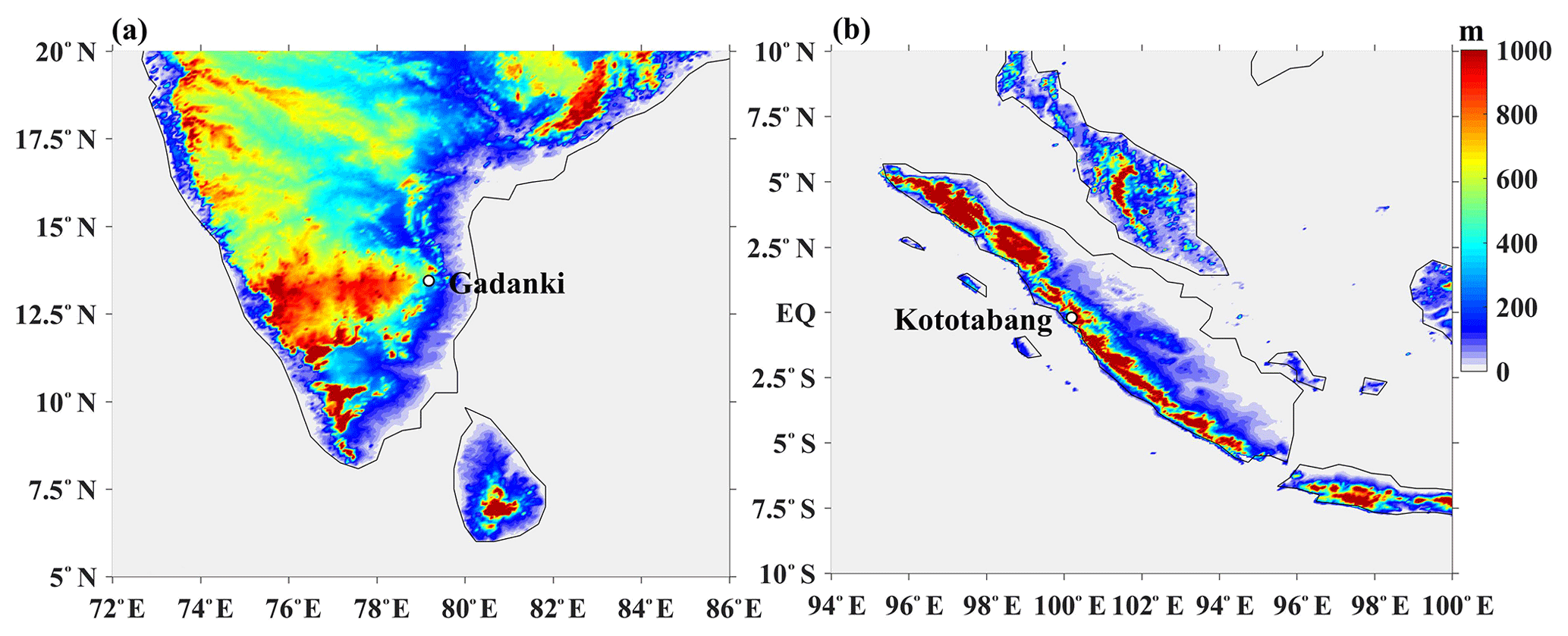
Figure 1 Topographical maps of the (a) IMSTR and (b) Kototabang EAR sites in mean sea level (MSL), generated by using the Shuttle Radar Topography Mission (SRTM) data (Farr et al., 2007). Dots on the map indicate the radar locations.

2 Data and methodology

2.1 Radar measurements

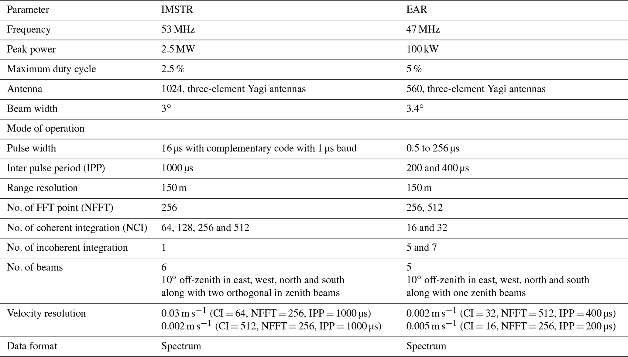
Remote-sensing measurements of w are obtained from the Indian Mesosphere–Stratosphere–Troposphere Radar (IMSTR) located at Gadanki, India (13.5^∘ N and 79.2^∘ E), and the Equatorial Atmosphere Radar (EAR) located at Kototabang, Indonesia (0.2 ^∘S and 100.2^∘ E). Figure 1a and b show the topography map of the location of both the radars, i.e., Gadanki and Kototabang, respectively, generated by using the Shuttle Radar Topography Mission (SRTM) data (Farr et al., 2007). Gadanki is located on the southern peninsula of tropical India, about 90 km off the east coast, and it is surrounded by hills. Kototabang is located in the western part of Sumatra island, and EAR is situated in the mountainous region, with the highest peak of about 2 km. Both the IMSTR and EAR are pulsed coherent radars operating at 53 and 47 MHz, respectively. These instruments are used to estimate w by measuring the Doppler shift in the vertical beam. The technical details and operational parameters of the IMSTR have been given by Rao et al. (1995), while those for the EAR have been given by Fukao et al. (2003). Both the radar specifications and parameters, including velocity resolution used for the present measurements, are listed in Table 1.

Table 1 The radar specifications and parameters used for the present measurements.

In the present study measurements of w from VHF radars are used to assess vertical motion between the surface and the lower stratosphere. Data collected from the IMSTR between 17:30 and 18:30 LT (LT = UTC + 05:30 h) from 1995 to 2015 are analyzed using the adaptive method (Anandan et al., 2001). This is the common operational mode of the IMSTR for deriving the winds and represents the only data available for such a long period of time. The three components of wind – zonal, meridional and vertical – can be computed with the radial velocity obtained in at least three non-coplanar directions. However, for the present analysis we have computed the w directly only using the vertical beam using Eq. (1):

$$\begin{array}{}\text{(1)}& w=(-\mathit{\lambda }/\mathrm{2})f_{\mathrm{d}},\end{array}$$

where λ is the radar wavelength (cm), and f_d is the Doppler velocity (Hz). In general, four to eight vertical profiles are averaged to create daily 16:30–17:30 IST (11:00–12:00 UTC) averaged profiles. Averaging is conducted using the arithmetic mean as it represents the central tendency, which is generally used for wind averaging. In a vertically pointing beam, the signal-to-noise ratio (SNR) decreases with height except in stable layers (like the tropopause) and in the presence of strong turbulence. Above 25 km, the SNR becomes constant in the absence of atmospheric signals. Data in this region can be therefore treated as noise and used to estimate the threshold SNR (Uma and Rao, 2009b). Noise levels estimated in this way lie between −17 and −19 dB with a 2σ value of 3 dB (where σ is the standard deviation). Thus data having SNR less than −15 dB are discarded from the present analysis. Data from intense convective days (checked for individual profiles), defined as w being less or greater than ± 1 m s⁻¹, are also discarded as these data severely bias the climatological mean w (e.g., Uma and Rao, 2009b). The data discarded are less than 1 % of the total data. Quality control metadata for the EAR measurements are available online (http://www.rish.kyoto-u.ac.jp/ear/data/index.html, last access: 10 May 2019). The EAR operates continuously, and this study uses hourly data (diurnal data of a single day) of w computed using the vertical beam (Eq. 1) from 2001 to 2015. The EAR data during convective periods are eliminated following the same criteria as for the IMSTR, a second screening step. Each full diurnal cycle (after removing convective profiles) is averaged and considered as a single daily profile for the EAR.

2.2 Accuracy and uncertainty in the w measured from radar

The assumption in the radar measurements of wind components is the spatial homogeneity in the given time frame, when we used three non-coplanar beams (e.g., two off-zenith and one vertical). Thus, to avoid the bias, we use only a vertical beam (Eq. 1) for the direct estimation of w, which also provides a better time resolution (Peterson and Balsley, 1979; Koscielny et al., 1984). The accuracy of the w measured made using the vertical beam of VHF radar depends on the alignment of the beam along the zenith direction. Any error in the beam pointing would mean that the line-of-sight velocity measured by the radar will have a component of the horizontal wind (Huaman and Balsley, 1996). The beam pointing error is found to be ± 0.2^∘ off-zenith, which was provided by calibrating the beam pointing with a known radio source Virgo A (Damle et al., 1991; Rao et al., 1995) and Cygnus A for EAR (Fukao et al., 2003). The uncertainty in the w due to beam pointing error by an angle θ with a horizontal wind u is given by u × sinθ. Thus, a horizontal wind of 10 m s⁻¹ and beam pointing error of 0.2^∘ yield 0.03 m s⁻¹ uncertainty in the w measured from VHF radar. The beam pointing accuracy can further be determined by comparing the w obtained using two orthogonal polarizations, i.e., east–west and north–south polarizations, which are phased independently. Significant correlation was observed between both the polarizations, suggesting that the radar measures the true w (Viswanathan et al., 1993). In addition, Rao et al. (2008) also estimated the vertical velocities from zenith beam and compared them with those estimated from 10^∘ off-zenith beams using IMSTR. The differences were observed to be meager, which shows that the error due to beam pointing is negligible.

Tilting of reflecting layers contributing to the diffuse reflection can also adversely bias the mean w (Röttger, 1980). These tilting layers can be due to the presence of Kelvin–Helmholtz instabilities (Muschinski, 1996) or gravity waves, which includes inertia–gravity waves and mountain waves and causes imbalance in the echo power between the two polarizations in the same plane (Yamamoto et al., 2003). Rao et al. (2008) estimated the echo power imbalance in the east–west and north–south polarizations for both EAR and IMSTR and found the difference to be within ± 1 dB, statistically indicating that the bias due to the tilting layers is negligible over both the locations.

Nastrom and VanZandt (1994) proposed that w can be biased by gravity waves. Thus, Rao et al. (2008) have investigated the biases caused by gravity waves by calculating the variances and found that downward-wind measurements below 10 km are essentially unaffected by gravity waves. It is also to be noted that the topography over the two locations can generate mountain waves if strong low-level winds are prevailing. Strong low-level winds are prevalent over Gadanki only from June to August, and during these months, there is a critical level existing between 6 and 7 km due to the presence of strong wind shear, which will not support the propagation of mountain waves to higher altitudes. This wind shear between 6 and 7 km exists throughout the year over Kototabang. Hence the effect of mountain waves on w will be minimal over both these locations. Their analysis clearly showed that the mean downward motion below 10 km and upward motion above 10 km are real and not caused by measurement biases and also that the known biases do not change the direction of the background w when measurements are averaged over a longer period of 10 years.

2.3 ERAi

ERA-Interim (ERAi) is a global reanalysis developed by the European Centre for Medium-Range Weather Forecasts (ECMWF). The data assimilation scheme used is 4D-Var (four-dimensional variational) of the upper-air atmospheric state and has effectively anchored both satellite and in situ observations. This scheme updates parameters that define bias corrections required for satellite observations. The model has improved in the representation of moist physical processes. Advances have also been made with respect to soil hydrology and snow in land surface models. The detail of the model is given in Dee et al. (2011). We use 6-hourly vertical velocities from the ERAi from 1995 to 2015. The grid resolution of ERAi is 0.75^∘ (latitude) × 0.75^∘ (longitude). The nearest grid points are taken for Gadanki (13.68^∘ N, 79.45^∘ E) and Kototabang (0.35^∘ S, 100.54^∘ E). ERAi has 37 pressure levels, from the surface up to 1 hPa. The pressure coordinate is converted into pressure height by using the hypsometric equation (Holton, 2004), which is followed for other reanalyses also. The difference between the pressure height and geometric height (radar measurements) is found to be < 100 m, which does not bias the results as the radar range resolution itself is 150 m. In the present analysis, we restrict the dataset up to 21 km, which is about 50 hPa, as that is the maximum radar range.

2.4 ERA5

ERA fifth generation (ERA5) is the atmospheric reanalysis produced by the ECMWF. It is an improved version of ERAi. The data assimilation scheme used is 4D-Var, and it assimilates the NCEP stage IV quantitative precipitation estimates produced over the USA by combining precipitation estimates from the Next-Generation Radar (NEXRAD) network with gauge measurements. The moist-physics scheme is improved by including freezing rain. The longwave radiation scheme is modified in ERA5. The evolution of the top soil layer, snow and sea ice temperatures is included. It uses observations from various satellites, which include upper air temperature, humidity and ozone. It also uses bending angles from GNSS. It provides much higher spatial (30 km) and temporal resolution (hourly) from the surface up to 80 km (137 levels). ERA5 also features much-improved representation, especially over the tropical regions of the troposphere, and better global balance of precipitation and evaporation. Many new data types not assimilated in ERAi are ingested in ERA5 (Hoffmann et al., 2019). The grid resolution of ERA5 is 0.28^∘ (latitude) × 0.28^∘ (longitude). The details are available in (Hersbach et al., 2020). We have taken hourly data from ERA5. The nearest grid points are again taken for Gadanki (13.63^∘ N, 79.31^∘ E) and Kototabang (0.14 ^∘S, 100.40^∘ E), and the data period is 2002–2015.

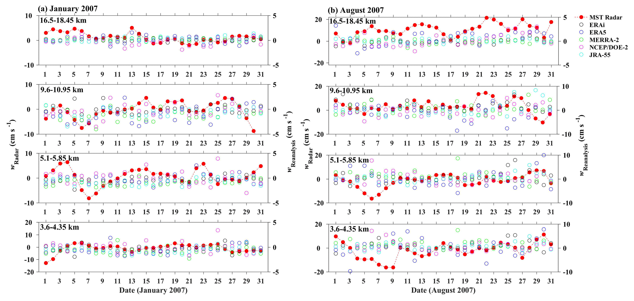
Figure 2 Intercomparison of layer-averaged daily w (12:00 UTC) measured from IMSTR with different reanalyses (ERAi, ERA5, MERRA-2, NCEP–DOE (R-2) and JRA-55) (12:00 UTC) over Gadanki for (a) January 2007 and (b) August 2007.

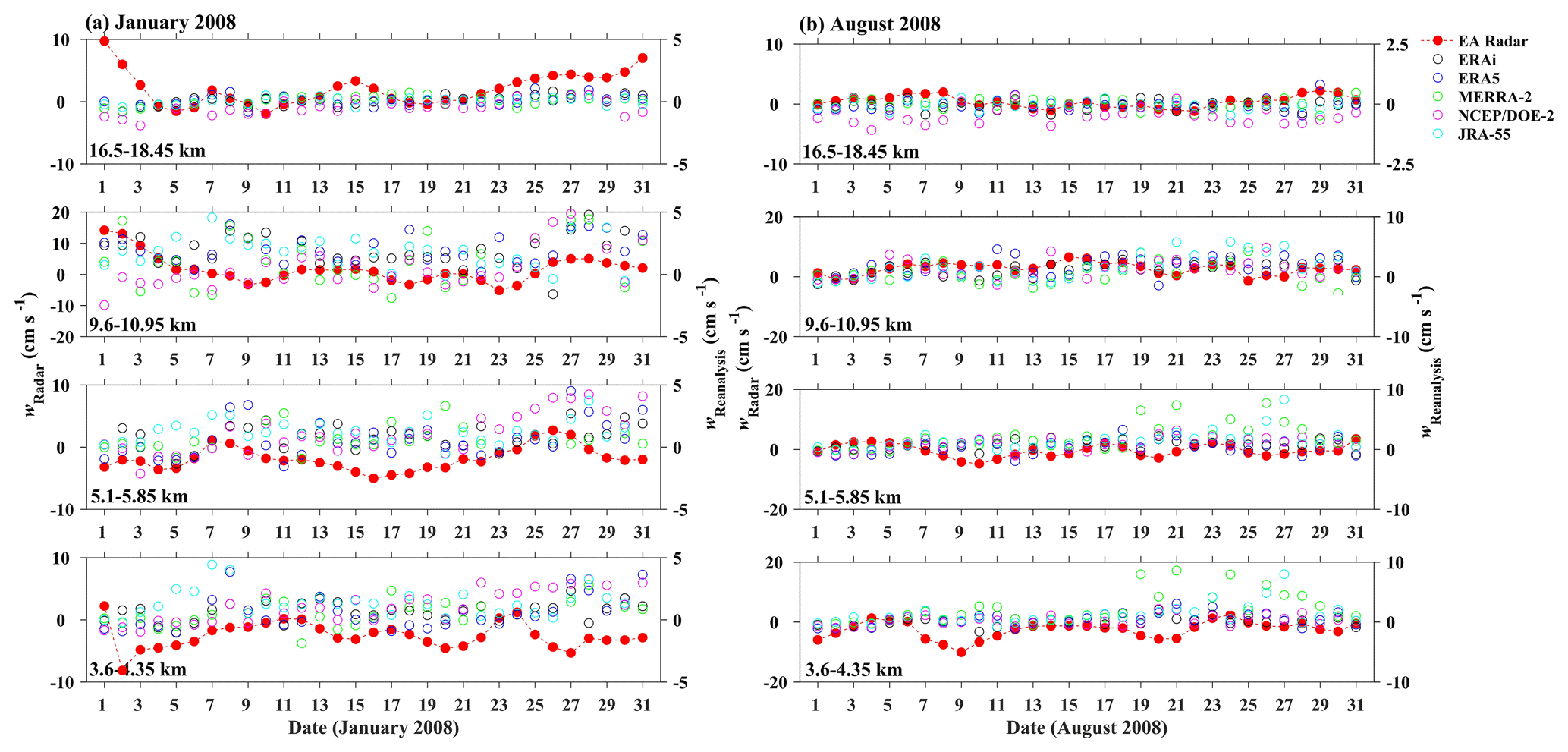
Figure 3 Same as Fig. 2 but for EAR over Kototabang. Please note that w is the diurnal mean (24 h mean) for both EAR and reanalyses for (a) January 2008 and (b) August 2008.

2.5 MERRA-2

The Modern-Era Retrospective analysis for Research and Applications, version 2 (MERRA-2) is the latest reanalysis of the modern satellite era produced by the National Aeronautics and Space Administration’s (NASA) Global Modeling and Assimilation Office (GMAO). The scheme used in MERRA-2 is an improved version of MERRA. It uses a three-dimensional variational (3D-Var) algorithm based on the grid point statistical interpolation and also uses an incremental analysis update. It assimilates bending angle observations and satellite radiances from both polar and geostationary infrared and microwave sounders. In addition it also assimilates water vapor and ozone. MERRA-2 includes aerosol analysis and provides data for 42 pressure levels from the surface to 0.01 hPa with a temporal resolution of 3 h and horizontal resolution of 0.5^∘ (latitude) × 0.625^∘ (longitude). We used MERRA-2 assimilation (ASM) data. Details have been provided by Gelaro et al. (2017). The nearest grid points are used for Gadanki (13.5^∘ N, 79.37^∘ E) and Kototabang (0.14^∘ S, 100.00^∘ E), with data spanning from 1995 to 2015.

2.6 NCEP–DOE (R-2)

The National Center for Atmospheric Research and Department of Energy (NCEP–DOE (R-2)) reanalysis is an updated version of NCEP-1 by fixing the known processing errors in NCEP-1. The variational scheme used is 3D-Var, and it provides more accurate pictures of soil wetness and near-surface temperature over land, the land surface hydrology budget, snow cover and radiation fluxes over the ocean. It is based on the NCEP operational model with a horizontal resolution of 209 km and 28 vertical levels. The temporal coverage is 4 times per day. NCEP–DOE (R-2) products are improved relative to NCEP-1, having fixed errors and updated parameterizations of physical processes, as evaluated by Kanamitsu et al. (2002). The grid resolution of NCEP–DOE (R-2) is 2.5^∘ (latitude) × 2.5^∘ (longitude). The data for the present study cover the period 1995 to 2015 and are extracted at the nearest grid points to Gadanki (12.5^∘ N, 77.5^∘ E) and Kototabang (0^∘, 100.00^∘ E).

2.7 JRA-55

The Japanese 55-year reanalysis (JRA-55) is an updated version of the earlier JRA-25 with new data assimilation and prediction systems (Kobayashi et al., 2015). New radiation schemes, higher spatial resolution and 4D-Var data assimilation with variational bias correction for satellite radiances have been used to generate the JRA-55 products. This reanalysis includes variation in greenhouse gas concentrations with time as well as the new representations of land surface parameters, aerosols, ozone and sea surface temperature. The grid resolution of JRA-55 is 1.25^∘ (latitude) × 1.25^∘ (longitude). The nearest grid points are taken for Gadanki (13.75^∘ N, 78.75^∘ E) and Kototabang (0, 100^∘ E), and the data period is 1995–2015.

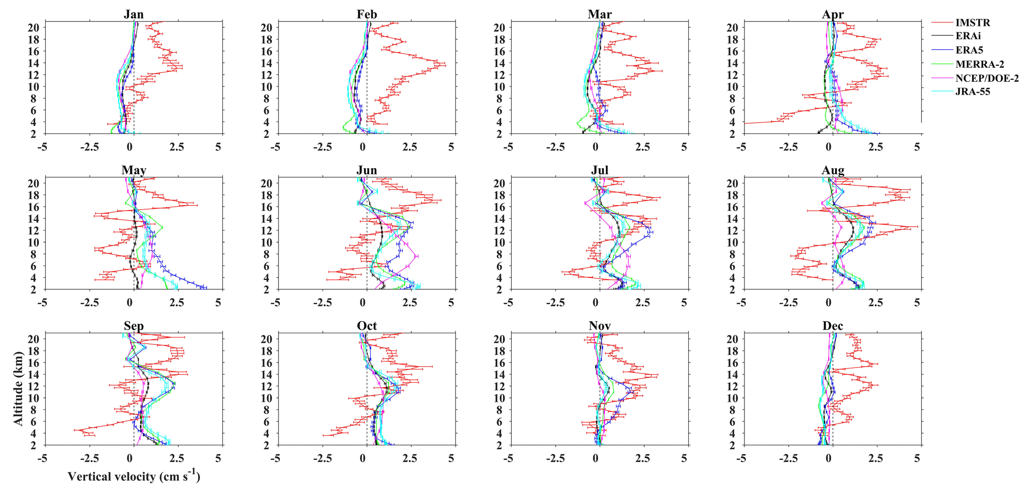
Figure 4 Climatological monthly mean altitude profile of w obtained from IMSTR and five reanalyses over Gadanki from 1995–2015. Horizontal lines indicate the standard error.

Figure 5 Same as Fig. 4 but from EAR over Kototabang from 2001 to 2015.

For all the reanalysis data, w (cm s⁻¹) is estimated using Eq. (2):

$$\begin{array}{}\text{(2)}& w=(-\mathrm{1}/g)\mathit{\omega }(RT/p),\end{array}$$

where ω is the vertical velocity in pressure coordinates (in Pa s⁻¹), T is the absolute temperature (K), p is the atmospheric pressure (hPa), and R (=287 J kg⁻¹ K⁻¹) is the gas constant for dry air. To compare measured vertical wind with the reanalysis products, we take the reanalysis data corresponding to 12:00 UTC for Gadanki and the daily mean for Kototabang. The details of the schemes used in reanalysis are provided in Table 2.

Mlawer et al. (1997)Morcrette (1991)Chou et al. (2002)Chou et al. (2002)Mlawer et al. (1997)Fouquart et al. (1990)Iacono et al. (2008)Chou and Suarez (1999)Briegleb (1992)Chou (1992)Chou and Lee (1996)Tiedtke (1989)Tiedtke (1989)Moorthi and Suarez (1992)Arakawa and Schubert (1974)Bechtold et al. (2004)Bechtold et al. (2008)Molod et al. (2015)Kawai and Inoue (2006)Campana and Cullather (1994)Dee et al. (2011)Hersbach et al. (2020)Gelaro et al. (2017)Kobayashi et al. (2015)Kanamitsu et al. (2002)

Table 2 Schemes of different reanalysis data used in the present study.

3 Results and discussion

Figure 2 shows the intercomparison of layer-averaged daily w measured from IMSTR with different reanalyses (ERAi, ERA5, MERRA-2, NCEP–DOE (R-2) and JRA-55) over Gadanki for (a) January 2007 and (b) August 2007. Both radar and all the reanalysis datasets are taken at 12:00 UTC, and the month and year are chosen in such a way so as to have maximum days of radar observations in two different seasons (winter and summer). Similarly, EAR observation is also compared with different reanalysis data but for January 2008 and August 2008, as shown in Fig. 3. However, both EAR and reanalysis data are diurnally averaged (24 h). It is observed that the magnitude of w measured from radar observations is an order of magnitude higher than the reanalysis data over both the locations (Gadanki and Kototabang). Most of the time, reanalysis data are comparable in direction with radar observations whenever updrafts are observed. It is also observed that there is mismatch between the w estimated in the different reanalyses.

Gage et al. (1992) described that averaging radar data for a long period of time can give a better measurement of w in clear-air conditions, and the authors have used 3 years data to arrive at the above conclusion. Thus in this context, we have taken 20 years of data for averaging. Figure 4 shows the climatological monthly mean altitude profile of w obtained from the IMSTR (observations) and the ERAi, ERA5, MERRA-2, NCEP–DOE (R-2) and JRA-55 reanalysis data over Gadanki. Although the magnitudes are of the same order between the observations and reanalyses, significant differences are identified in the figures. Convective days are discarded from the radar data (observations) as mentioned in the previous section, and those days are also eliminated from all reanalysis datasets. The quantitative differences may be attributed to the spatial averaging implicit in the reanalysis products, whereas the radar measurements are for a single point. Thus we only discuss the tendency of w as it is used to represent the variation in w rather than its magnitude. The IMSTR observations show updrafts between 8 and 20 km from December to April, with the largest values in the tropical tropopause layer (TTL; 12–16 km). These features are not reproduced by any of the reanalyses, which all show downdrafts from December to April between 1 km and the tropopause level (mean tropopause is ∼ 16.5 km). By comparison, downdrafts are observed in the IMSTR below 6 km in April, which may be attributed to pre-monsoon (March-May) precipitation and evaporation (Uma and Rao, 2009a). w in ERAi differs in both magnitude and direction from other reanalyses, especially in the lower troposphere from March to June. Meanwhile, the magnitude of w in ERA5 is a little larger than that in the other reanalyses from May to June. Updrafts are observed in the TTL by the IMSTR during June, when all reanalyses show similar features but only located below the TTL. During July and August both the radar observations and the reanalyses show updrafts in the vicinity of the TTL. Updrafts are observed in the TTL from September to November, but the peak in the updrafts is shifted lower than that observed by the IMSTR. Below 8 km, the IMSTR shows downdrafts from April to October. The reanalysis data are unable to reproduce downdrafts above 2 km.

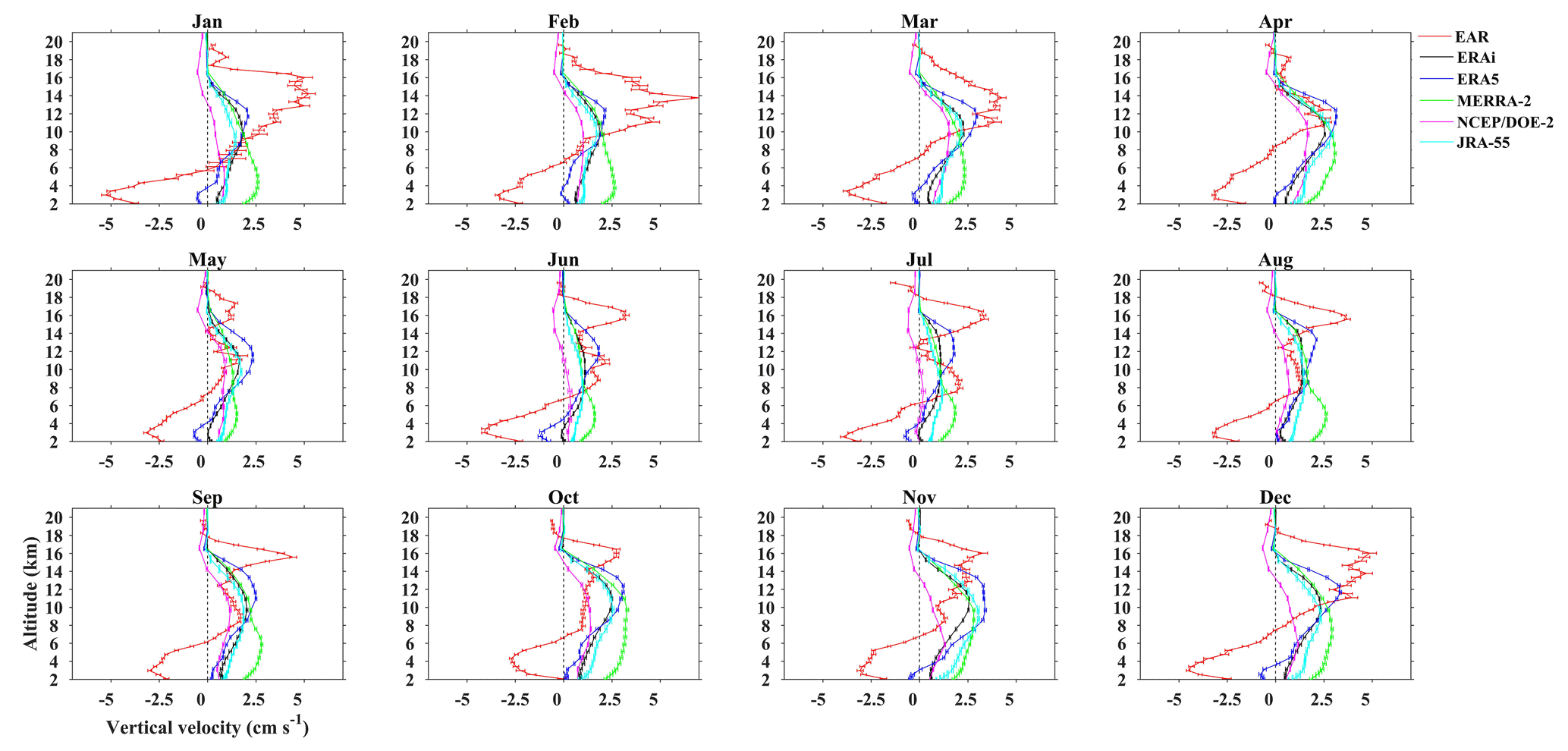
We have also analyzed w from the EAR (Kototabang), where the observations are available for the full diurnal cycle (measurements of hourly averages for 24 h of observations). All reanalysis data over Kototabang are averaged for the full diurnal cycle. Figure 5 shows the monthly mean climatology of daily mean w from the EAR observations and the five reanalyses over Kototabang. All the reanalyses agree well with each other over Kototabang. The updrafts in the TTL are well reproduced by all five reanalyses, although the magnitude and vertical location of the maximum in w remain lower than observed. However none of the reanalyses reproduce the downdrafts. A distinct bimodal distribution in w from May to September (two peaks between 8–10 and 14–17 km) with a local minimum between 12 and 13 km is observed in the EAR measurements which are not observed in the reanalysis. The magnitudes of both updrafts and downdrafts are larger than those observed over Gadanki. JRA-55 produces the largest w among the reanalyses. The monthly means show significant differences in the direction of w between the observations and the reanalyses below 6 km.

Gage et al. (1992) studied the long-term diurnal variability in w at Christmas Island (2^∘ N) and found that the w varies between ± 4 cm s⁻¹. The observations showed updrafts below 4 km, downdrafts between 4–14 km and updrafts above 12 km. Gage et al. (1991) have explained that the downward motion in the troposphere is consistent with a heat balance in the clear air between adiabatic warming of descending air and radiative cooling to space. The ascending motion in the upper troposphere and lower stratosphere is due to large diabatic heating caused by ice particles in the cirrus. Rao et al. (2008) have shown the long-term (11 years) mean of w over Gadanki and Kototabang and found that w varies between −0.3 and +0.6 cm s⁻¹. The authors observed downdrafts below 6 km and updrafts above it in all the seasons. The mean patterns of the w profile observed by radars over all the tropical sites (i.e., Christmas Island, Gadanki and Kototabang) show similar characteristics and explain that the vertical transport of air from the troposphere to the lower stratosphere is a two-step process as discussed by Rao et al. (2008). Uma and Rao (2009b) have reported the diurnal variation (using hourly data) of w in different seasons, although their observations had only one to two diurnal cycles per month over Gadanki. They found significant variations in the seasonal variability in diurnal cycle as large as ± 6 cm s⁻¹ over Gadanki using IMSTR. The present observations are limited to 16:30 to 17:30 IST, with all reanalysis data over Gadanki taken at 12:00 UTC (17:30 IST). Thus, time-averaged climatological-mean biases can be neglected.

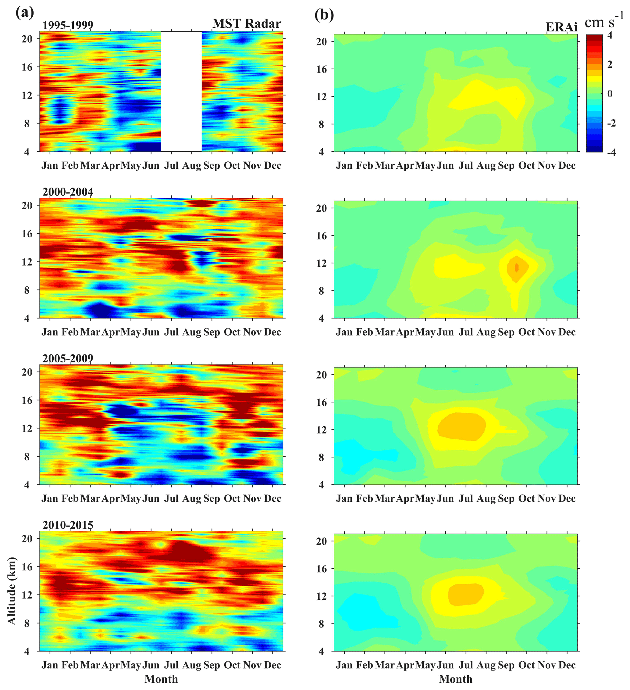
Figure 6 Monthly mean w obtained from (a) IMSTR and (b) ERAi for a 5-year interval (from top to bottom) over Gadanki (12:00 UTC).

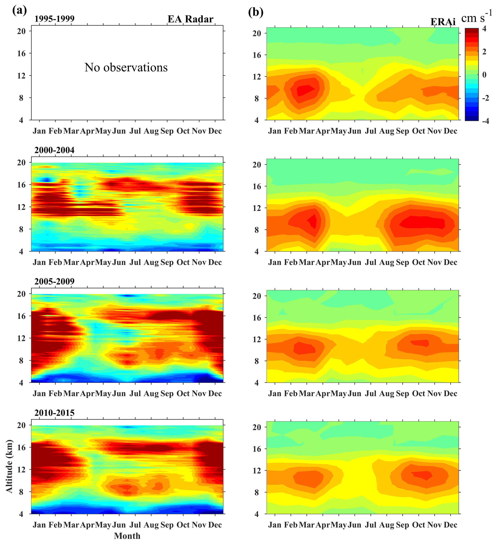
To establish the robustness of the results we have used different averaging procedures to assess the consistency of the variability in w at monthly scales. Monthly mean climatological profiles of w from radar observations and various reanalyses over Gadanki and Kototabang are shown in Fig. A1 in the Appendix. Downdrafts in the troposphere are not captured by any of the reanalyses over either location. By contrast, updrafts in the TTL are generally reproduced in the monthly mean, though their magnitudes are often underestimated by the reanalyses. ERAi underestimates the magnitude of both updrafts and downdrafts over Gadanki, while NCEP–DOE (R-2) underestimates the magnitude of updrafts over Kototabang. Monthly means calculated over 5-year periods from both the radar data and ERAi are shown in Fig. 6 for Gadanki and Fig. 7 for Kototabang. The reanalysis shows similar behavior to the overall climatology in each 5-year average. The overall patterns of updrafts and downdrafts in the radar measurements of w are also similar, indicating a consistent performance of the radar over the full 20-year analysis period.

Figure 7 Same as Fig. 6 but for diurnal mean from EAR over Kototabang.

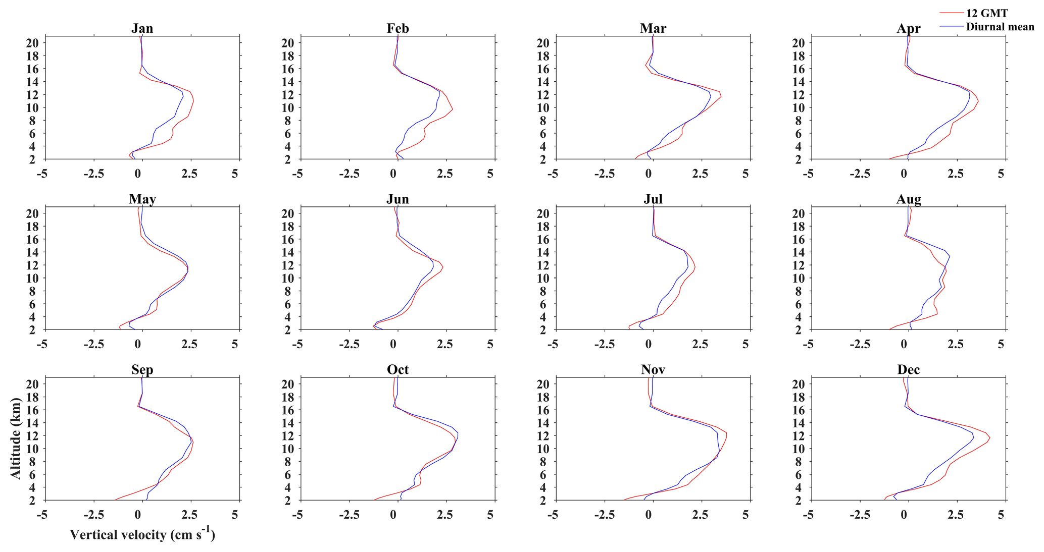
To further elucidate potential biases in the results due to averaging, we have taken ERA5 at 12:00 UTC and compared it to the daily mean (obtained by averaging w at different times of the day) to show that the sampling restrictions at Gadanki do not bias the results obtained. Figures 8 and 9 show the mean w obtained at 12:00 UTC and also the mean obtained by averaging hourly analyses for each day for Gadanki and Kototabang, respectively. ERA5 is chosen for this evaluation as the data are available at 1 h intervals. The analysis shows some differences in the magnitude of w, with 12:00 UTC generally showing larger magnitudes compared to the daily means over Gadanki (although no such systematic differences are observed in Kototabang). The directional tendencies are also similar in both the profiles at both locations. This analysis shows that the results are not biased by taking data only at 12:00 UTC over Gadanki.

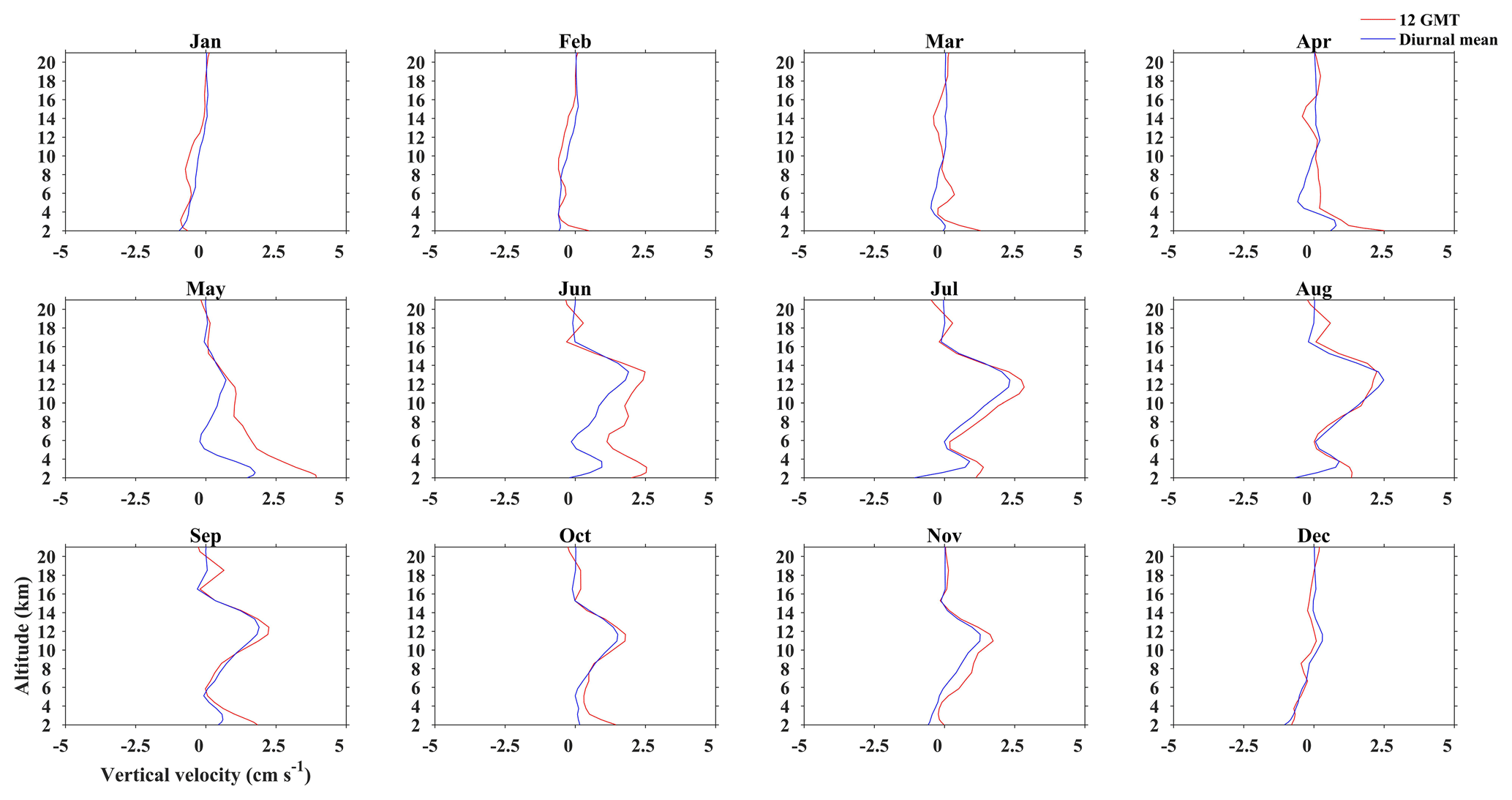
Figure 8 Height profile of w at 12:00 UTC and diurnal mean (with 1 h resolution) over Gadanki extracted from ERA5 during 1995–2015 (highest available time resolution).

Figure 9 Same as Fig. 8 but for Kototabang during 2001–2015.

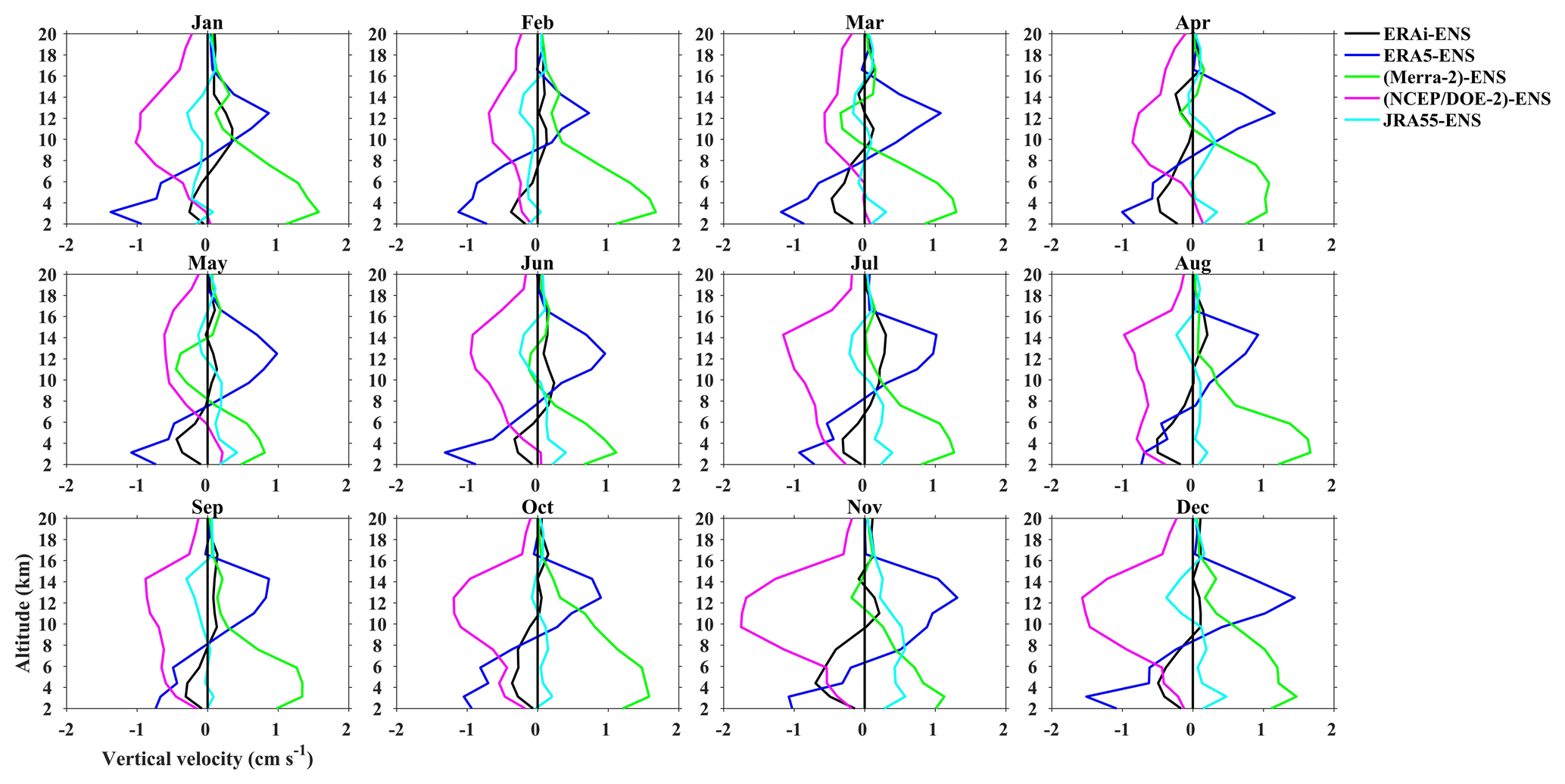
Our analysis to this point shows the level of consistency between the features observed by the radar and those in the reanalysis. To further understand the relative differences among the reanalyses we perform a monthly mean comparative analysis among the reanalyses, as shown in Figs. 10 and 11 for Gadanki and Kototabang, respectively. We take an ensemble mean of all the five reanalyses and then subtract the ensemble mean from each reanalysis. The differences are less than ± 0.5 cm s⁻¹ during December–January–February (DJF; winter). During March–April–May (MAM), the difference between the ensemble and reanalysis shows ± 2 cm s⁻¹ below 5 km. Below 5 km, NCEP–DOE (R-2) and ERAi are less, whereas ERA5, MERRA-2 and JRA-55 are more than the ensemble. The difference above 6 km is less than ± 0.5 cm s⁻¹. JRA-55 shows a good comparison with the ensemble, and above 10 km the differences in all the reanalyses are minimal with the ensemble. During the monsoon (June–July–August, JJA), the difference is comparatively high in June compared to July and August. NCEP–DOE (R-2) and ERA5 are more, and other reanalyses are less than the ensemble; however during July and August NCEP–DOE (R-2) is less in the upper troposphere (10–18 km). MERRA-2 and ERAi show a good comparison with respect to the ensemble during July and August; JRA-55 also shows a good comparison in addition to MERRA-2 and ERAi. During SON, the differences are comparatively less than during MAM and JJA. The difference is less than ± 0.5 cm s⁻¹ during October and November, except in September between 10 and 15 km, where ERA5 and MERRA-2 are more, and ERAi and NCEP–DOE (R-2) are less than the ensemble. In general, ERA5 and NCEP–DOE (R-2) show considerably more difference with the ensemble, and other reanalyses (ERAi, MERRA-2 and JRA-55) compare well with the ensemble.

Figure 10 Comparison of relative differences in w between the reanalysis ensemble mean and each reanalysis for Gadanki from 1995 to 2015. Individual monthly differences are estimated and then averaged for each month.

Figure 11 Same as Fig. 10 but for Kototabang from 2001 to 2015.

Over Kototabang (Fig. 11), it is interesting to note the difference between the ensemble and that different reanalyses show a consistent pattern during all the months. JRA-55 and ERAi show good comparison with the ensemble as the differences are less than ± 0.2 cm s⁻¹ in all the seasons, except in November, where it exceeds ± 0.5 cm s⁻¹ in the lower and middle troposphere. MERRA-2 is more, and NCEP–DOE (R-2) is less than the ensemble in all the height regions. ERA5 is less below 10 km and more above with respect to the ensemble.

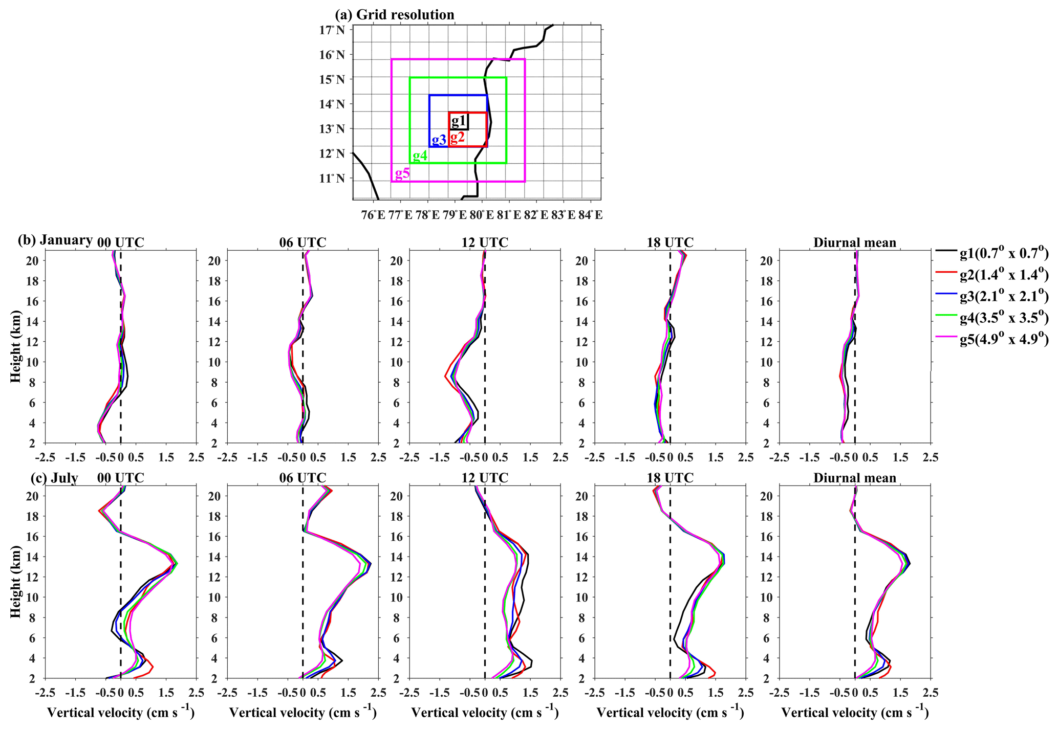
Figure 12 (a) Map for spatial averaging (grid resolution) and height profiles of w for different spatial averaging at 00:00, 06:00, 12:00 and 18:00 UTC, respectively, for ERAi reanalysis during 2007.

There may be some probable reasons for the differences in the w measured by observations and those retrieved from reanalysis. The main bias in w might occur in the reanalysis due to the following: (1) indirect estimation of omega, (2) local topography influence in the reanalysis, (3) use of different schemes in the boundary layer, (4) interactions between subgrid physical parameterizations and the large-scale flow, and (5) spatial and temporal sampling. However, it is difficult to address the above issues other than the spatial and temporal sampling. To elucidate the spatiotemporal averaging on the vertical velocity, we have chosen different grid resolutions with Gadanki as a centroid, and the map is shown in Fig. 12a. G1 to G5 represent different grid resolutions, varying from 0.7 to 5^∘. The data chosen are for January and July 2007 from ERAi. The height profile of w at different grid resolutions and times is shown in Fig. 12b for January and in Fig. 12c for July. It is observed that the grid resolution does not have any influence on the w. However, a significant change is observed between 00:00 and 12:00 UTC in the month of January which affected the diurnal mean in w (shown in the last panel). The same is not reflected in the month of July. The result shows that narrowing down the reanalysis data spatially (reducing the horizontal sampling) will not improve the retrieval of w in any reanalysis.

The direction of w is an essential metric for comparing the reanalysis with the observations. We therefore show the directional tendencies of reanalysis data relative to the radar measurements. The directional tendencies would be 100 % when all radar measurements in a certain height range are reproduced by a reanalysis in terms of the w direction. Figure 13a shows the directional tendencies based on the IMSTR and the reanalyses over Gadanki, while Fig. 13b shows the directional tendencies based on the EAR and the reanalyses over Kototabang. The directional tendency is calculated at each height for every month when the radar or reanalysis data exceed 0.1 cm s⁻¹ in either direction. The directional tendency for each month is estimated and then aggregated into seasons. These directional tendencies are given in terms of percentage of occurrence with respect to height. The tendency is calculated separately for updrafts and downdrafts.

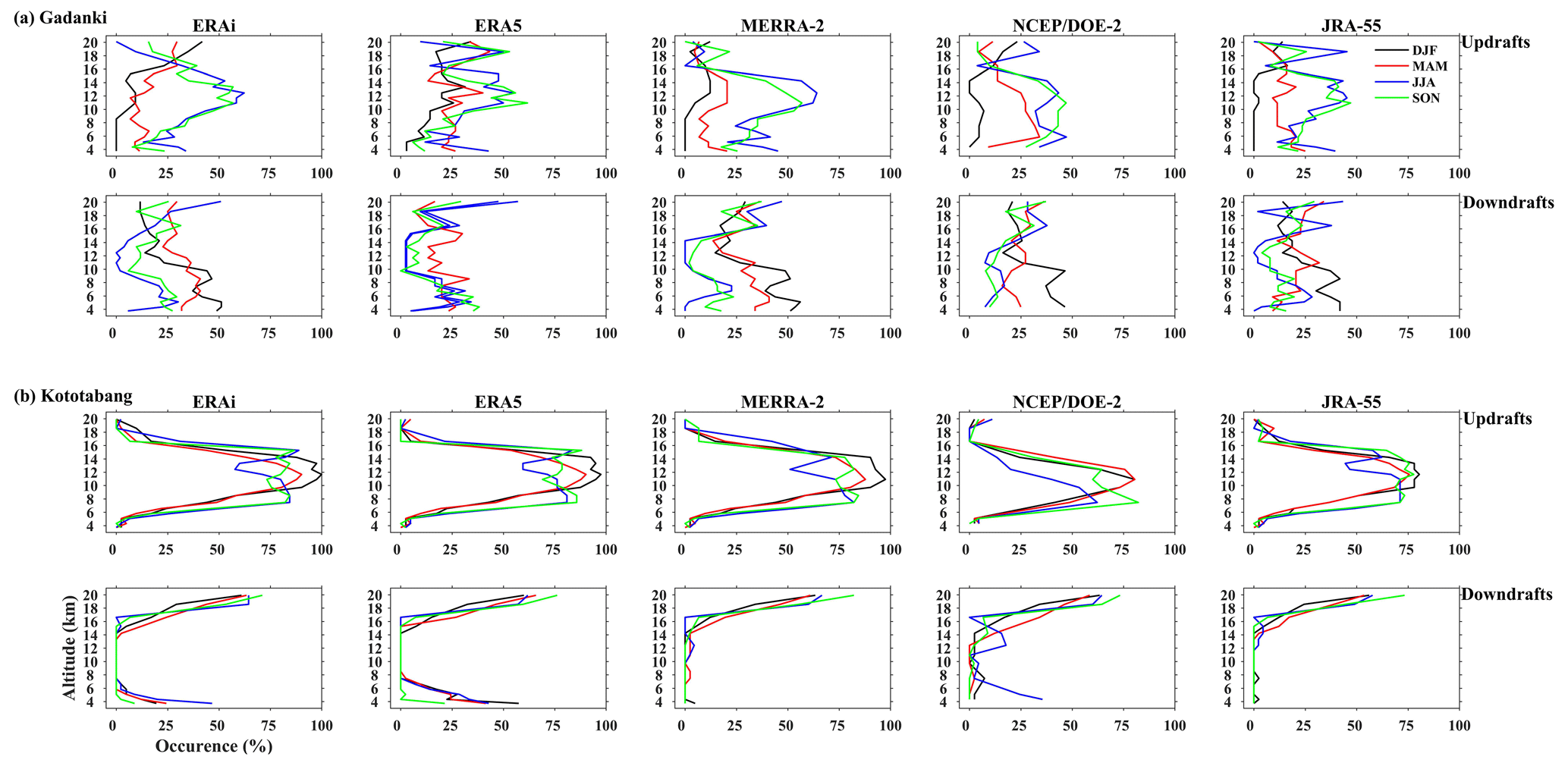
Figure 13 Comparison of directional tendency of w between the radars and various reanalysis datasets for (a) Gadanki (1995–2015) and (b) Kototabang (2001–2015). Updrafts are shown in rows 1 and 3, and downdrafts are shown in rows 2 and 4 (for details see text).

Over Gadanki during DJF all reanalyses produce updrafts (simultaneously by both radar and reanalysis) less than 10 % of the time throughout the profile. During MAM these ratios increase to around 15 %, with NCEP–DOE (R-2) reproducing updrafts about 25 % of the time. During JJA and SON, the percentage occurrence increases with the height from 25 % to a maximum of 50 % between 12 and 14 km. The percentage occurrence of updraft then decreases from 14 to 20 km. This tendency trend is similar for all reanalyses. The maximum ratio of updrafts over Gadanki is located between 12 and 15 km altitude. The percentage occurrence of downdrafts over Gadanki is also less than 50 % at all levels. During DJF and MAM the reanalyses reproduce downdrafts 40 % to 50 % of the time, a much higher frequency than that for updrafts (< 10 %). This fraction decreases above 10 km. By contrast, the percentage of downdrafts reproduced during JJA and SON is less than that of updrafts, with frequencies less than 25 % at all levels during these seasons.

Over Kototabang the percentage occurrence of updrafts increases with height in all seasons, reaching a maximum of 75 %–90 % between 10 and 14 km. Above 14 km the percentage decreases to a minimum of 5 % at 19 km. Updrafts are rarely reproduced by the reanalysis altitudes less than 4 km. It is important to note that none of the reanalyses reproduce daily mean downdrafts exceeding 1 cm s⁻¹ except ERAi and ERA5, which reproduced downdrafts below 6 km. The percentage of downdrafts increases above 17 km, where it reaches a maximum, and shows occurrence frequencies around 65 % to 75 % above 18 km.

4 Conclusions

The present study assesses the vertical motion (w) in reanalyses against radar observations in the troposphere and lower stratosphere from the convectively active regions Gadanki and Kototabang. The assessment is carried out for five different reanalyses: ERAi, ERA5, MERRA-2, NCEP–DOE (R-2) and JRA-55. Measurements were collected using VHF radar at both locations. We have used 20 years of data from Gadanki and 17 years of data from Kototabang. The following points summarize the results of this unique study:

1. The magnitude of w obtained from reanalyses is underestimated by 10 %–50 % relative to the radar observations.

2. Observations over Gadanki showed updrafts from 8 to 20 km year-round. All the reanalyses only reproduced this feature during JJA and SON, when magnitudes were larger than 0.5 cm s⁻¹ in the reanalysis data. However, the vertical location of the updrafts differs between the observations and the reanalyses. Downdrafts below 8 km are not captured well by reanalysis data.

3. Over Kototabang, all five reanalyses did not consistently reproduce downdrafts below 8 km in all months. Updrafts in the upper troposphere and lower stratosphere are captured well; however, the peak in the vertical distribution of w is different as over Gadanki.

4. Intercomparison between the ensemble and data of each reanalysis shows that the ERAi, MERRA-2 and JRA-55 compare well with the ensemble compared to ERA5 and NCEP–DOE (R-2). Analysis also showed that the reduction in spatial sampling in all the reanalysis data does not significantly improve the magnitude of w.

5. Assessment of directional tendencies shows that updrafts are reproduced reasonably well in the data of all five reanalyses, but downdrafts are not reproduced at all.

The present analysis reveals that downdrafts are not well captured in the data of all five reanalyses. The location of the largest updrafts is also shifted lower in reanalyses than in the observations. It is to be noted that w measured from radar is limited over a geographical area, and thus the results may be valid in a limited region. However, the results demonstrate how approaches to generating global reanalysis products (encompassing different models, assimilation methods, spatial resolution, etc.) can impact estimates of w. Hence, reanalysis data should be used with caution for representing various atmospheric-motion calculations (viz. diabatic heating, convection, etc.) that mainly depend on the direction of w.

Appendix A

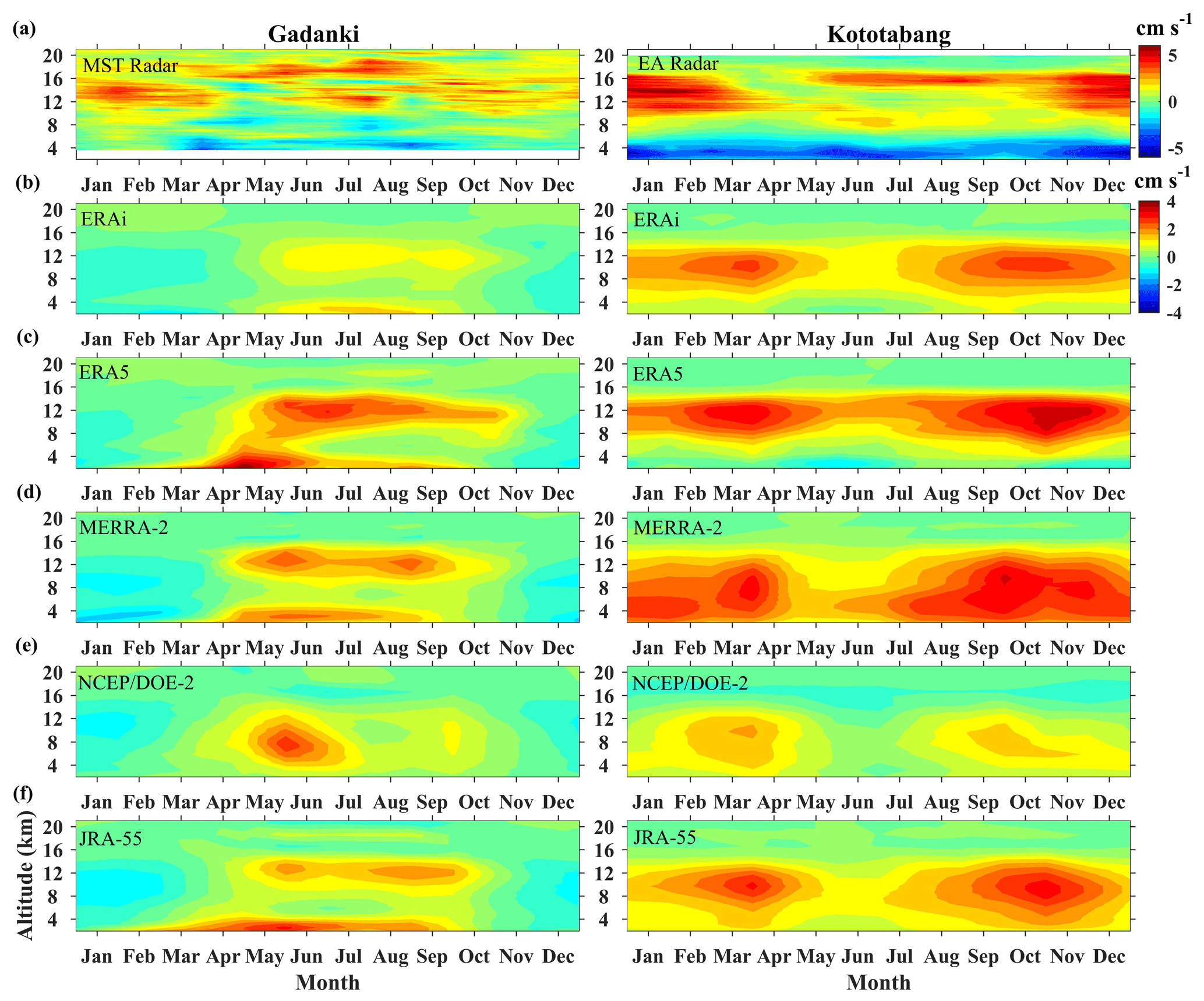
Figure A1 Monthly mean climatology of w obtained from (a) radars, (b) ERAi, (c) ERA5, (d) MERRA-2, (e) NCEP–DOE (R-2) and JRA-55 over Gadanki (left) (1995–2015), and Kototabang (right) (2001–2015). Gadanki data are at 12:00 UTC and Kototabang data are diurnal mean.