Regional CO₂ fluxes from 2010 to 2015 inferred from GOSAT XCO₂ retrievals using a new version of the Global Carbon Assimilation System

Satellite retrievals of the column-averaged dry air mole fractions of CO₂ (XCO₂) could help to improve carbon flux estimation due to their good spatial coverage. In this study, in order to assimilate the GOSAT (Greenhouse Gases Observing Satellite) XCO₂ retrievals, the Global Carbon Assimilation System (GCAS) is upgraded with new assimilation algorithms, procedures, a localization scheme, and a higher assimilation parameter resolution. This upgraded system is referred to as GCASv2. Based on this new system, the global terrestrial ecosystem (BIO) and ocean (OCN) carbon fluxes from 1 May 2009 to 31 December 2015 are constrained using the GOSAT ACOS (Atmospheric CO₂ Observations from Space) XCO₂ retrievals (Version 7.3). The posterior carbon fluxes from 2010 to 2015 are independently evaluated using CO₂ observations from 52 surface flask sites. The results show that the posterior carbon fluxes could significantly improve the modeling of atmospheric CO₂ concentrations, with global mean bias decreases from a prior value of 1.6 ± 1.8 ppm to −0.5 ± 1.8 ppm. The uncertainty reduction (UR) of the global BIO flux is 17 %, and the highest monthly regional UR could reach 51 %. Globally, the mean annual BIO and OCN carbon sinks and their interannual variations inferred in this study are very close to the estimates of CarbonTracker 2017 (CT2017) during the study period, and the inferred mean atmospheric CO₂ growth rate and its interannual changes are also very close to the observations. Regionally, over the northern lands, the strongest carbon sinks are seen in temperate North America, followed by Europe, boreal Asia, and temperate Asia; in the tropics, there are strong sinks in tropical South America and tropical Asia, but a very weak sink in Africa. This pattern is significantly different from the estimates of CT2017, but the estimated carbon sinks for each continent and some key regions like boreal Asia and the Amazon are comparable or within the range of previous bottom-up estimates. The inversion also changes the interannual variations in carbon fluxes in most TransCom land regions, which have a better relationship with the changes in severe drought area (SDA) or leaf area index (LAI), or are more consistent with previous estimates for the impact of drought. These results suggest that the GCASv2 system works well with the GOSAT XCO₂ retrievals and shows good performance with respect to estimating the surface carbon fluxes; meanwhile, our results also indicate that the GOSAT XCO₂ retrievals could help to better understand the interannual variations in regional carbon fluxes.

1 Introduction

Atmospheric carbon dioxide (CO₂) is one of the most important greenhouse gases, and fossil fuel burning and land use change are mostly responsible for its increase from the preindustrial concentration. Terrestrial ecosystems and oceans play very important roles in regulating the atmospheric CO₂ concentration. Over the past 50 years, about 60 % of the anthropogenic CO₂ emissions have been absorbed by the terrestrial ecosystems and oceans (IPCC, 2014); however, their carbon uptakes have significant spatial differences and interannual variations (Bousquet et al., 2000; Takahashi et al., 2009; Piao et al., 2020). Therefore, it is very important to quantify the global and regional carbon fluxes.

Atmospheric inversion is an effective method for estimating the surface CO₂ fluxes using globally distributed atmospheric CO₂ concentration observations (Enting and Newsam, 1990; Gurney et al., 2002). It has robust performance on global- or hemisphere-scale carbon budget estimates (Houweling et al., 2015), but on regional scales, due to the uneven distribution of in situ observations, the reliability of inversion results varies greatly in different regions. Generally, the inversions have large uncertainties in tropics, Southern Hemisphere oceans and most continental interiors such as South America, Africa, and boreal Asia (Peylin el al., 2013). Satellite observation has a better spatial coverage, especially over remote regions, and studies show that it can be used to improve the carbon flux estimates (e.g., Chevallier et al., 2007; Miller et al., 2007; Hungershoefer et al., 2010). The Greenhouse Gases Observing Satellite (GOSAT) (Kuze et al., 2009) – the first satellite mission dedicated to observing CO₂ from space – was launched in 2009. Many inversions have utilized the GOSAT retrievals for column-averaged dry air mole fractions of CO₂ (XCO₂) to infer surface carbon fluxes (e.g., Basu et al., 2013; Maksyutov et al., 2013; Saeki et al., 2013a; Chevallier et al., 2014; Deng et al., 2014, 2016; Wang et al., 2018a, 2019). Takagi et al. (2011) found that GOSAT XCO₂ retrievals could significantly reduce the uncertainties in estimates of surface CO₂ fluxes for regions in Africa, South America, and Asia, where the sparsity of the surface monitoring sites is most evident. Basu et al. (2013) showed that assimilating only GOSAT data can effectively reproduce the observed CO₂ time series at the surface and Total Carbon Column Observing Network (TCCON) sites in the tropics and the northern extra-tropics, but this enhances seasonal cycle amplitudes in the southern extra-tropics. Wang et al. (2019) also showed that GOSAT XCO₂ retrievals can effectively improve carbon flux estimation, and the performance of the inversion with GOSAT data only was comparable to the one using in situ observations. Meanwhile, based on the inversions with GOSAT XCO₂ retrievals, Liu et al. (2018) quantified the impacts of the 2011 and 2012 droughts on terrestrial ecosystem carbon uptake anomalies over the contiguous US, Deng et al. (2016) compared the distributions of drought and posterior carbon fluxes in South America for the 2010–2012 period, and Detmers et al. (2015) studied the impact of the strong La Niña episode on the carbon fluxes in Australia from the end of 2010 to early 2012. To date, most studies have focused on the impact of GOSAT XCO₂ retrievals on the inversion of surface carbon fluxes; however, in many regions, there are still large divergences for carbon sinks between different inversions with the same GOSAT data or between inversions with GOSAT and in situ observations (e.g., Chevallier et al., 2014; Feng et al., 2016; Wang et al., 2018a). Moreover, although some studies have reported the impact of drought or extreme wetness on the changes in carbon fluxes using inversions based on GOSAT, few studies have comprehensively investigated the impacts of GOSAT data on the interannual variations in inverted land sinks in different regions (Feng et al., 2017; Byrne et al., 2019).

In this study, we present a 6-year inversion from 2010 to 2015 for the global and regional carbon fluxes using only the GOSAT XCO₂ retrievals. The Global Carbon Assimilation System (GCAS) is employed to conduct this inversion, which was developed in China in 2015 (Zhang et al., 2015) and updated in this study with a new scheme to assimilate XCO₂ retrievals. The inverted multiyear averaged carbon fluxes for the globe, global land and ocean, each TransCom region (Gurney et al., 2002), and some other key areas are shown and compared with previous top-down and bottom-up (Jiang et al., 2016) estimates. The estimated interannual variations in carbon fluxes in each TransCom region are given and discussed against changes in drought and leaf area index (LAI). This paper is organized as follows: Sect. 2 details the GCASv2 system as well as the prior fluxes, GOSAT retrievals, and uncertainty settings. Section 3 briefly introduces the experimental design. Results and discussions are presented in Sect. 4, and conclusions are given in Sect. 5.

2 Methods and data

2.1 A new version of the Global Carbon Assimilation System (GCASv2)

Figure 1 shows the flow chart of the GCASv2 system. In each data assimilation (DA) window, there are two steps. In the first step, the prior fluxes of X^b in each grid are independently perturbed with a Gaussian random distribution and put into a global atmospheric chemical transport model to simulate CO₂ concentrations, which are then sampled according to the locations and times of CO₂ observations. The sampled data are used in the assimilation module together with the CO₂ observations to generate the optimized fluxes of X^a. In the second step, the atmospheric transport model is run again using the optimized fluxes of X^a in order to generate new CO₂ concentrations for the initial field of the next DA window. Using this method, if the flux in one window is overestimated for some reason, it will affect the concentrations of the next window; thus, the posterior flux of the next window will compensate for the overestimation. This DA flow chart is different from the previous version of GCAS (GCASv1), which runs the atmospheric transport model only once, and optimizes the fluxes and the initial field of the next window synchronously: in each window, there is relatively perfect initial field (directly optimized using observations), the inversions of each window are independent, and the amount of overestimation or underestimation in one window will continue to accumulate until the end, leading to an overall overestimation or underestimation. In addition, due to the relatively perfect initial field, the differences between the simulated and observed concentrations are only contributed by the errors in the prior fluxes of current window, resulting in a relatively smaller model–data mismatch, so as to weaken the assimilation benefits on fluxes.

Figure 1 Flow chart of the GCASv2 system.

The perturbation of X^b represents the uncertainty of the prior carbon flux, which is calculated using the following function:

$$\begin{array}{}\text{(1)}& X_i^b=X_{\mathrm{0}}^b+\mathit{\lambda }\times {\mathit{\delta }}_i\times X_{\mathrm{0}}^b,i=\mathrm{1},\mathrm{2},\mathrm{\dots },N,\end{array}$$

where δ_i represents random perturbation samples, which are drawn from Gaussian distributions with a mean of zero and a standard deviation of one; N is the ensemble size; and λ is a set of scaling factors, which represents the uncertainty of each prior flux. In GCASv1, λ is defined in different land and ocean areas based on 22 TransCom regions (Gurney et al., 2002) and 19 Olson ecosystem types, as in CarbonTracker (CT, Peters et al., 2007). This means that in the same area, the error of a prior flux is the same. Through assimilation, the flux will be integrally enlarged or reduced. In GCASv2, we change to use λ in each grid, meaning that for each grid, the perturbations of prior fluxes are independent. In addition, the grid cell of λ is different from those of the prior flux and the transport model, which could be set freely. $X_{\mathrm{0}}^{\mathrm{b}}$ is the prior carbon flux. Generally, there are four types of carbon fluxes, namely the terrestrial ecosystem (BIO) carbon flux (i.e., net ecosystem exchange = ecosystem respiration − gross primary production; NEE = ER − GPP), atmosphere and ocean (OCN) carbon exchange, fossil fuel and cement production (FOSSIL) carbon emission, and biomass burning (FIRE) carbon emission, which are used to drive the transport model to simulate the atmospheric CO₂ concentration. In general, FOSSIL and FIRE fluxes are assumed to have no errors, and only BIO and OCN fluxes are optimized in an assimilation system (e.g., Gurney et al., 2002; Peters, et al., 2007; Nassar et al., 2011; Jiang et al., 2013; Chevallier, et al., 2019). In GCASv1, only the BIO flux was treated as a state vector and optimized, and the OCN flux was directly from the CarbonTracker (CT) output produced by the US National Oceanic and Atmospheric Administration (NOAA). In GCASv2, the state vector is set to be an optional item. Four schemes are set: the first one is the same as the previous version – only the BIO flux is optimized (Formula 2); the second one is the same as the general scheme – namely both BIO and OCN fluxes are state vectors (Formula 3); the third one is that BIO, OCN, and FOSSIL fluxes are optimized at the same time (Formula 4); and the fourth one is that only the net flux is optimized (Formula 5). In this study, the second scheme was selected.

$$\begin{array}{}\text{(2)}& {\displaystyle }\begin{array}{rl}{X}_i^b& =\left(X_{\mathrm{bio}}^b+{\mathit{\lambda }}_{\mathrm{bio}}\times {\mathit{\delta }}_{i,\mathrm{bio}}\times X_{\mathrm{bio}}^b\right)\\ & +X_{\mathrm{ocn}}^b+X_{\mathrm{fossil}}^b+X_{\mathrm{fire}}^b,i=\mathrm{1},\mathrm{2},\mathrm{\dots },N\end{array}\text{(3)}& {\displaystyle }\begin{array}{rl}{X}_i^b& =\left(X_{\mathrm{bio}}^b+{\mathit{\lambda }}_{\mathrm{bio}}\times {\mathit{\delta }}_{i,\mathrm{bio}}\times X_{\mathrm{bio}}^b\right)\\ & +\left(X_{\mathrm{ocn}}^b+{\mathit{\lambda }}_{\mathrm{ocn}}\times {\mathit{\delta }}_{i,\mathrm{ocn}}\times X_{\mathrm{ocn}}^b\right)\\ & +X_{\mathrm{fossil}}^b+X_{\mathrm{fire}}^b,i=\mathrm{1},\mathrm{2},\mathrm{\dots },N\end{array}\text{(4)}& {\displaystyle }\begin{array}{rl}{X}_i^b& =\left(X_{\mathrm{bio}}^b+{\mathit{\lambda }}_{\mathrm{bio}}\times {\mathit{\delta }}_{i,\mathrm{bio}}\times X_{\mathrm{bio}}^b\right)\\ & +\left(X_{\mathrm{ocn}}^b+{\mathit{\lambda }}_{\mathrm{ocn}}\times {\mathit{\delta }}_{i,\mathrm{ocn}}\times X_{\mathrm{ocn}}^b\right)\\ & +\left(X_{\mathrm{fossil}}^b+{\mathit{\lambda }}_{\mathrm{fossil}}\times {\mathit{\delta }}_{i,\mathrm{fossil}}\times X_{\mathrm{fossil}}^b\right)\\ & +X_{\mathrm{fire}}^b,i=\mathrm{1},\mathrm{2},\mathrm{\dots },N\end{array}\text{(5)}& {\displaystyle }\begin{array}{rl}{X}_i^b& =\left(X_{\mathrm{bio}}^b+X_{\mathrm{ocn}}^b+X_{\mathrm{fossil}}^b+X_{\mathrm{fire}}^b\right)\\ & +{\mathit{\lambda }}_{\mathrm{netflux}}\times {\mathit{\delta }}_{i,\mathrm{netflux}}\\ & \times \left(X_{\mathrm{bio}}^{\mathrm{b}}+X_{\mathrm{ocn}}^b+X_{\mathrm{fossil}}^b+X_{\mathrm{fire}}^b\right),i=\mathrm{1},\mathrm{2},\mathrm{\dots },N\end{array}\end{array}$$

For the CO₂ observations, in GCASv1, only the flask and in situ observations were assimilated. In GCASv2, we added a module to use satellite XCO₂ retrievals. With this module, simulated CO₂ concentration profiles are converted to XCO₂ concentrations, and users can choose to assimilate flask and in situ observations alone, satellite XCO₂ retrievals alone, or simultaneously assimilate these two types of data. The simulated CO₂ concentration profiles are mapped into the satellite retrieval levels and then vertically integrated based on a satellite averaging kernel according to the following equation (Connor, et al., 2008):

$$\begin{array}{}\text{(6)}& {{\mathrm{XCO}}_{\mathrm{2}}}^m={{\mathrm{XCO}}_{\mathrm{2}}}^{\mathrm{b}}+{\sum }_j{h}_j{k}_j\left(\mathbf{A}\left(x\right)-y_{\mathrm{b},j}\right),\end{array}$$

where j denotes the retrieval level, x is the simulated CO₂ profile, A(x) is a mapping matrix, XCO${}_{\mathrm{2}}^{\mathrm{b}}$ is the prior XCO₂, h_j is a pressure weighting function, and k_j and y_b,j are the satellite column-averaging kernel and the prior CO₂ profile for retrieval, respectively.

To reduce the computational cost and the influence of representative errors, a “super-observation” approach is also adopted in GCASv2 based on the optimal estimation theory (Miyazaki et al., 2012). A super-observation is generated by averaging all observations located within the same model grid within a DA window. We assume that the observation errors of different stations at different times are independent of each other. The standard deviation of the jth observation y_j is r_j. The super-observation y_new, standard deviation r_new, and corresponding simulations x_new,i from one perturbed prior flux $X_i^{\mathrm{b}}$ are calculated as follows:

$$\begin{array}{}\text{(7)}& {\displaystyle }\mathrm{1}/r_{\mathrm{new}}^{\mathrm{2}}={\sum }_{j=\mathrm{1}}^m\mathrm{1}/r_j^{\mathrm{2}},\text{(8)}& {\displaystyle }{y}_{\mathrm{new}}={\sum }_{j=\mathrm{1}}^m{w}_j{y}_j/{\sum }_{j=\mathrm{1}}^m{w}_j,\text{(9)}& {\displaystyle }{x}_{\mathrm{new},i}={\sum }_{j=\mathrm{1}}^m{w}_j{x}_{j,i}/{\sum }_{j=\mathrm{1}}^m{w}_j,\end{array}$$

where $w_j=\mathrm{1}/r_j^{\mathrm{2}}$ is the weighting factor, and m is the number of observations within a super-observation grid. The super-observation error decreases as the number of observations used for the super-observation increases.

2.1.1 Ensemble square root filter (EnSRF) assimilation algorithm

Besides the local ensemble transform Kalman filter (LETKF), which has been implemented in GCASv1 in order to avoid storing and inverting very large matrices during analysis, in GCASv2, we added another assimilation algorithm, namely the ensemble square root filter (EnSRF) algorithm (Whitaker and Hamill, 2002), which has been successfully used in CT (Peters et al., 2005). EnSRF obviates the need to perturb the observations, in contrast to the traditional ensemble Kalman filter (EnKF) algorithm, and assimilates observations in a sequential way. It shows better performance than the method to assimilate observations simultaneously as long as the observation errors are uncorrelated (Houtekamer and Mitchell, 2001). The implementation process and setup are detailed below.

After obtaining an ensemble of state vectors as described in Sect. 2.1, ensemble runs of the atmospheric transport model are conducted to propagate these errors in the model with each ensemble sample of a state vector. The background error covariance P^b is calculated based on the forecast ensemble from Eq. (10):

$$\begin{array}{}\text{(10)}& P^{\mathrm{b}}={\displaystyle \frac{\mathrm{1}}{n-\mathrm{1}}}{\sum }_{i=\mathrm{1}}^n\left(X_i^b-{\stackrel{\mathrm{‾}}{X}}^b\right){\left(X_i^b-{\stackrel{\mathrm{‾}}{X}}^b\right)}^T,\end{array}$$

where ${\stackrel{\mathrm{‾}}{X}}^b$ represents the mean of the ensemble samples. Based on the background error covariance, the response of the uncertainty in the simulated concentrations to the uncertainty in emissions is obtained. Combing observational vector y, the state vector is updated according to the following formulations:

$$\begin{array}{}\text{(11)}& {\displaystyle }{\stackrel{\mathrm{‾}}{X}}^a={\stackrel{\mathrm{‾}}{X}}^b+K\left(\mathit{y}-H{\stackrel{\mathrm{‾}}{X}}^b\right),\text{(12)}& {\displaystyle }K=P^{\mathrm{b}}{H}^T{\left(H{P}^{\mathrm{b}}{H}^T+R\right)}^{-\mathrm{1}},\text{(13)}& {\displaystyle }\mathit{\delta }{X}_i^a=\mathit{\delta }{X}_i^b-\stackrel{\mathrm{̃}}{K}H\mathit{\delta }{X}_i^b.\end{array}$$

Sequential assimilation and independent observations are also employed:

$$\begin{array}{}\text{(14)}& \stackrel{\mathrm{̃}}{\mathbf{K}}=(\mathrm{1}+\sqrt{R/H{P}^{\mathrm{b}}{H}^T+R}{)}^{-\mathrm{1}}\mathbf{K},\end{array}$$

where H is the observation operator that maps the state variable from model space to observation space; K is the Kalman gain matrix of the ensemble mean depending on background and observation error covariance R, representing the relative contributions to analysis; $\stackrel{\mathrm{̃}}{\mathbf{K}}$ is the Kalman gain matrix of the ensemble perturbation; and emission perturbations after inversion $\mathit{\delta }{X}_i^a$ can then be calculated. At the analysis step, the ensemble mean ${\stackrel{\mathrm{‾}}{X}}^a$ is taken as the best estimate of the carbon flux.

2.1.2 Atmospheric transport model

As in GCASv1 (Zhang et al., 2015), the Model for OZone And Related chemical Tracers, version 4 (MOZART-4; Emmons et al., 2010) is adopted as the atmospheric transport model in GCASv2. MOZART-4 is a flexible model, can be run at essentially any resolution, and can be driven by essentially any meteorological data set and with any emission inventory (Emmons et al., 2010). In this system, we preset two horizontal resolutions for MOZART-4 runs: one is approximately 2.8^∘ × 2.8^∘, with transport model grids of 128 × 64, and the another is approximately 1.0^∘ × 1.0^∘, with 360 × 180 model grids. In the vertical direction, we use 28 layers. The ERA-Interim reanalysis data sets from the European Centre for Medium-Range Weather Forecasts (ECMWF) are used to drive the model. ERA-Interim data sets include as many as 128 meteorological variables and have a maximum spatial resolution of approximately 80 km (T255 spectral) on 60 vertical levels from the surface up to 0.1 hPa. Only the variables required for MOZART-4 with a spatial resolution of 1.0^∘ × 1.0^∘ and 28 vertical levels for 3-D variables from the surface to approximately 2.5 hPa are selected in this system. The selected variables and vertical levels are shown in Tables S1 and S2 in the Supplement.

2.1.3 DA window and localization

The DA window is set to 1 week in GCASv2, which is the same as before. Theoretically, a longer DA window is better, because CO₂ is a stable species. Thus, the longer the window, the farther CO₂ will be transported. In this way, more observation stations will sense the flux change in one area; therefore, more observations can be used to optimize the flux of that place. For this reason, many previous ensemble-based assimilation systems have used a longer DA window (e.g., Peters et al., 2005; Feng et al., 2009; Jacobson et al., 2020). However, the farther that the observation station is from the source, the weaker signal that the stations can sense. Bruhwiler et al. (2005) clearly showed that a pulse traveling from a faraway place would contribute relatively little signal compared with recent pulses from nearby source regions. In addition, limited by the EnKF method, this weak signal will be masked by the method's own unphysical signal (spurious correlation); in order to reduce this influence, we must increase the ensembles, thereby greatly increasing the computational cost. Miyazaki et al. (2011) tested the differences between 3 d and 7 d DA windows and noted that more observational data will be available to constrain the surface flux when using a longer DA window, but a longer window can make the effect of model error more obvious. Thus, the assimilation result can be improved as long as the observations with spurious correlations can be neglected. However, spurious correlations can be more serious with increases in the DA window due to the limited number of ensembles. As a result, a longer window system is not necessarily better than a shorter window system. To avoid the influence of spurious signals, Kang et al. (2012) used a very short DA window (6 h) in their assimilation system (LETKF_C) and pointed out that the flux inversion with a long window (3 weeks) is not as accurate as that obtained with a 6 h DA window, particularly in smaller-scale structures. During the development of GCASv1, Zhang et al. (2015) tested different DA windows and found that the longer the window, the larger the optimized terrestrial carbon sink, resulting in a smaller optimized annual atmospheric CO₂ growth rate (AGR) compared with the observed rate. Considering the fact that, due to the release of satellite XCO₂ retrievals like GOSAT and Orbiting Carbon Observatory-2 (OCO-2), the atmospheric CO₂ observations and coverage have increased significantly compared with what was available in the past, we no longer need to extend the DA window to include more observational data. Figure S2 shows the mean super-observation (see Sect. 2.1, only GOSAT XCO₂) numbers during the study period that each grid (3^∘ × 3^∘) could have within a 1-week DA window and localization scale (3000 km, see the next paragraph). In most land areas and pantropical waters, each grid can already have more than three super-observations. On average, each grid over the land could have four super-observations. In this study, two sensitivity tests in 2010 were conducted using 2- and 4-week DA windows and the same localization scale; the results of these tests are shown in Table S4. When the length of the DA window was increased from 1 week to 4 weeks, the respective mean super-observation number increased from four to nine and the respective inverted global BIO flux increased from −4.16 to −4.49 Pg yr⁻¹, resulting in a larger deviation of the simulated and observed AGR and larger simulation error against the surface observations. Therefore, we still use the 1-week DA window in GCASv2.

As previously discussed, there are inevitably spurious correlations in the EnKF method. Therefore, a localization scale, which determines that only measurements located within a certain distance (cutoff radius) of a grid point will influence the analysis of this grid, must be set to reduce the effect of spurious correlations. The localization technique in this study is based on both the distance between one site and one grid cell of λ, and the linear correlation coefficient between the simulated concentrations and the perturbed fluxes for each parameter (λ)–observation pair. If the distance is less than 500 km and the correlation coefficient is greater than zero, the observations will be accepted for assimilation; if the distance is greater than or equal to 500 km and less than 3000 km and the relationship between a parameter deviation and its modeled observational impact is statistically significant (p<0.05), the relationship is retained. Otherwise, the relationship is assumed to be spurious noise. On average, 87 % of the observations were spurious noise and were removed in this study. The spurious observations will increase the inverted global land sink and enlarge the deviation of the simulated and observed AGR. For different TransCom regions, the impact for the inverted BIO fluxes could be in the range of −32 % to 40 % (Table S4). The scale of 3000 km is set simply according to the globally averaged 80 m wind speed during the day (4.96 m s⁻¹, Archer and Jacobson, 2005) and the length of the DA window (1 week).

2.2 Prior carbon fluxes

As described in Sect. 2.1, there are four types of prior carbon fluxes in GCASv2. In this study, FOSSIL carbon emissions, which are an average of the Carbon Dioxide Information Analysis Center (CDIAC) product (Andres et al., 2011) and the Open-source Data Inventory of Anthropogenic CO₂ (ODIAC) emission product (Oda et al., 2018), are obtained from NOAA's CT, version 2017 (CT2017, Peters et al., 2007, with updates documented at http://carbontracker.noaa.gov, last access: 4 March 2020). The FIRE CO₂ emissions, which are the average of the Global Fire Emissions Database version 4.1 (GFEDv4) (Randerson et al., 2017) and the Global Fire Emission Database from the NASA Carbon Monitoring System (GFED_CMS), are also taken from CT2017. The OCN CO₂ exchange is from the pCO₂-Clim prior of CT2017, which is derived from the Takahashi et al. (2009) climatology of seawater pCO₂. In addition, as shown in Fig. 7 of the CT2017 release documentation (https://www.esrl.noaa.gov/gmd/ccgg/carbontracker/CT2017/, last access: 3 March 2020), there are no data in many seas such as the Sea of Japan, the Mediterranean, the Gulf of Mexico, and the East China Sea; therefore, the fluxes in 2009 modeled using the global ocean circulation and biogeochemistry model (OPA-PISCES–T) (Buitenhuis et al., 2006; Jiang et al., 2013) are used to fill the areas with no data.

The BIO carbon flux, which is one of the essential prior carbon fluxes in an assimilation system, was simulated using the Boreal Ecosystems Productivity Simulator (BEPS) model (Chen et al., 1999; Ju et al., 2006) in this study. BEPS is a process-based, remote sensing data driven, and mechanistic ecosystem model. In this study, the BEPS model was run starting from 2000. To simplify the initialization, the initial values of the different carbon pools are from a previous BEPS simulation (Chen et al., 2019). In short, all carbon pools were assumed to be in a state of dynamic equilibrium from 1901 to 1910, and all carbon pools were determined by solving a set of equations describing the dynamics of carbon pools (Chen et al., 2003). The simulation was then forwarded using historical data. Due to the lack of historical remotely sensed LAI data, the averaged LAI from 1982 to 1986 represented that over the 1901–1981 period. All of our initial carbon pools were then set to the states of carbon pools in 2000 according to Chen et al. (2019). The BEPS model was also driven by the 1^∘ × 1^∘ ERA-Interim reanalysis data sets, including relative humidity, wind speed, air temperature, incoming solar radiation, and total precipitation. The other data include LAI data and clumping index. The LAI was inverted from surface reflectance data sets of Moderate Resolution Imaging Spectroradiometer (MODIS) (Liu et al., 2012), and the clumping index was derived from the MODIS Bidirectional Reflectance Distribution Function (BRDF) products, which provided the finest pseudo-multiangular data for the land surface, according to the normalized difference between hotspot and darkspot (NDHD) index (Chen et al., 2005; He et al., 2012).

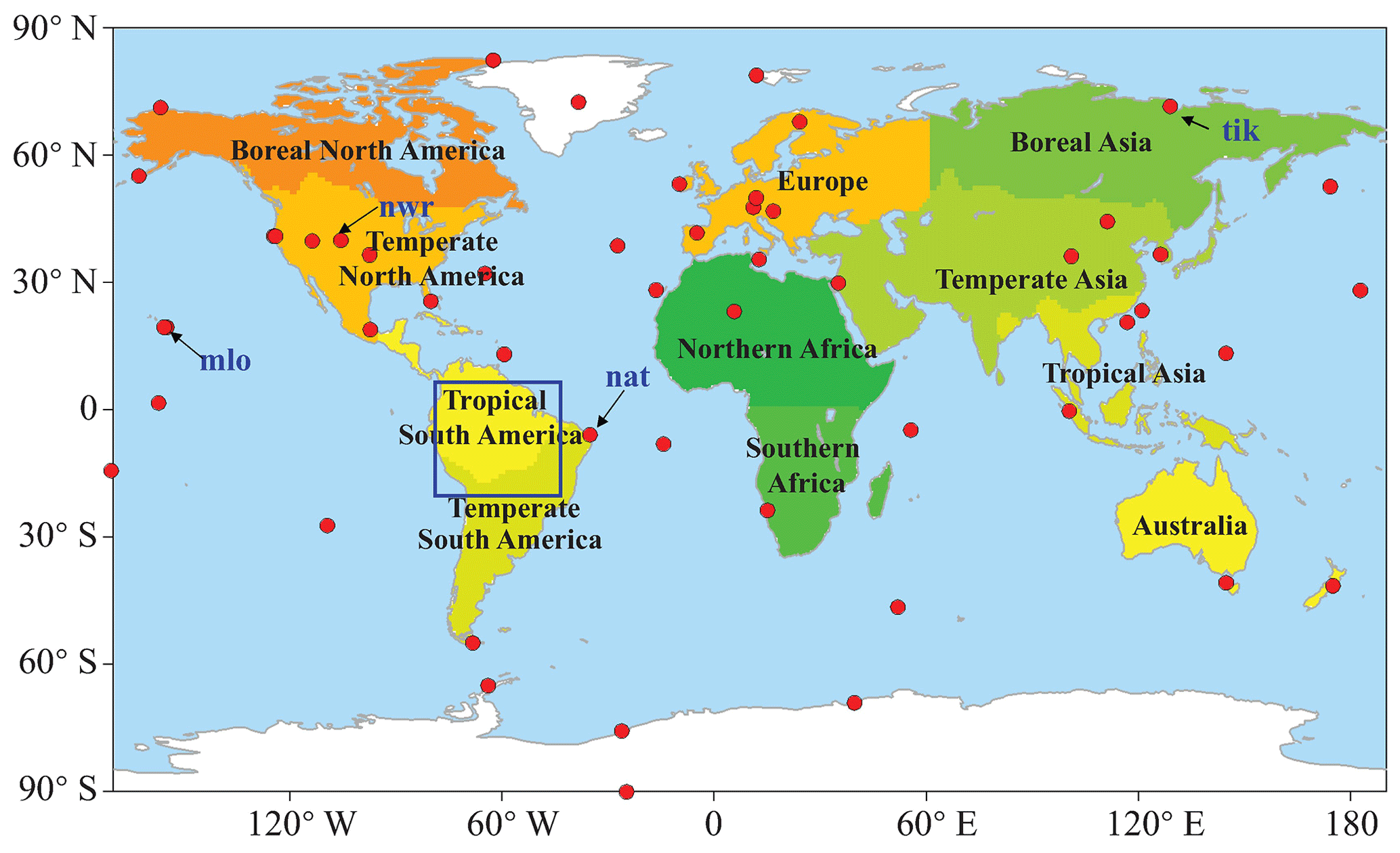
Figure 2 Distributions of the observation sites used in this study. Red solid circles are the 52 surface flask sites used for the evaluations, the shading shows the 11 TransCom regions, and the blue rectangle shows the Amazon region, which is defined following Botta et al. (2012).

2.3 GOSAT XCO₂ retrievals

The GOSAT XCO₂ retrievals of the Atmospheric CO2 Observations from Space (ACOS) Version 7.3 Level 2 Lite product (O'Dell et al., 2012; Crisp et al., 2012) at the pixel level during the May 2009–December 2015 period is used in this study (this product is bias corrected) (Wunch et al., 2011). In order to achieve the most extensive spatial coverage with the assurance of using the best quality data available, the XCO₂ retrievals are filtered with the warn_levels and xco2_quality_flag parameters, which are provided along with the product, prior to being used in the inversion system. Only the data with xco2_quality_flag greater than zero are selected. The selected data are then divided into three groups according to the value of warn_levels: warn_levels less than 8, warn_levels greater than 9 and less than 12, and warn_levels greater than 13. The group with the lowest warn_levels has the best data quality, whereas the group with the highest values has the worst data quality. The pixel data are then averaged within the 1^∘ × 1^∘ grid cell, and only the group with best data quality in each grid is selected and then averaged. The other variables like the column-averaging kernel and the retrieval error (Formula 6), which are provided along with the XCO₂ product, are also dealt with using the same method. This process is the same as Wang et al. (2019).

2.4 Evaluation data and method

Generally, direct validation of the optimized flux is impossible; instead, we indirectly evaluate the posterior flux by comparing the forward-simulated atmospheric CO₂ mixing ratios against measurements (e.g., Jin et al., 2018; Wang et al., 2019; Feng et al., 2020). First, the simulated XCO₂ are compared against the corresponding GOSAT XCO₂ retrievals to test the effectiveness of the assimilation system (see Sect. 2.3 for the description of the GOSAT XCO₂ retrieval). Second, Surface CO₂ observations used for independent evaluations in this study are obtained from the obspack_co2_1_GLOBALVIEWplus_v5.0_2019-08-12 product. It is a subset of the Observation Package (ObsPack) data product (ObsPack, 2019) and contains a collection of discrete and quasi-continuous measurements at surface, tower, and ship sites, which are contributed by national and universities laboratories around the world. In this study, surface CO₂ measurements from 52 flask sites are selected to evaluate the posterior CO₂ concentrations, which are all provided by the NOAA Global Monitoring Laboratory (with a lab number of 1 in each filename). The locations of the 52 sites can be found in Fig. 2, and the corresponding site codes as well as the latitude and longitude information are listed in Table S3 in the Supplement.

During the evaluation, four basic statistical measures, namely the mean bias (BIAS), mean absolute error (MAE), root mean square error (RMSE), and correlation coefficient (CORR), are calculated against the surface CO₂ observations and GOSAT XCO₂ retrievals, respectively. The BIAS, MAE, RMSE, and CORR reflect the overall model tendency, both the model bias and error variance, and the linear correspondence between the modeled and observed values or retrievals, respectively. The functions of these four basic statistical measures are expressed as follows:

$$\begin{array}{}\text{(15)}& {\displaystyle }\mathrm{BIAS}={\displaystyle \frac{\mathrm{1}}{M}}{\sum }_{j=\mathrm{1}}^M\left(x_j-y_j\right)=\stackrel{\mathrm{‾}}{y}-\stackrel{\mathrm{‾}}{x};\text{(16)}& {\displaystyle }\mathrm{MAE}={\displaystyle \frac{\mathrm{1}}{M}}{\sum }_{j=\mathrm{1}}^M\mathrm{|}{x}_j-y_j\mathrm{|};\text{(17)}& {\displaystyle }\mathrm{RMSE}=\sqrt{{\displaystyle \frac{\mathrm{1}}{M}}{\sum }_{j=\mathrm{1}}^M{\left(x_j-y_j\right)}^{\mathrm{2}}};\text{(18)}& {\displaystyle }\mathrm{CORR}={\displaystyle \frac{{\sum }_{j=\mathrm{1}}^M\left(x_j-\stackrel{\mathrm{‾}}{x}\right)\left(y_j-\stackrel{\mathrm{‾}}{y}\right)}{\sqrt{{\sum }_{j=\mathrm{1}}^M{\left(x_j-\stackrel{\mathrm{‾}}{x}\right)}^{\mathrm{2}}}\sqrt{{\sum }_{j=\mathrm{1}}^M{\left(y_j-\stackrel{\mathrm{‾}}{y}\right)}^{\mathrm{2}}}}}.\end{array}$$

Here, x_j and y_j denote the modeled and the observed values or retrievals, respectively, at the jth out of M records, and the overbars denote averages.

3 Experimental design

The assimilation system was run from 1 May 2009 to 31 December 2015. Two forward simulations with the prior and posterior fluxes were also conducted from 1 May 2009 to 31 December 2015, respectively. For both assimilation and forward runs, the initial field of 3-D CO₂ concentrations at 00:00 UTC on 1 May 2009 was also from the CT2017 product, and the MOZART-4 model was run with the 2.8^∘ × 2.8^∘ resolution. The first 8 months are considered as a spin-up run, and the results from 1 January 2010 to 31 December 2015 are analyzed and evaluated in this study.

During the assimilation, the resolution of λ is the same as the transport model. For the state vector, the second scheme (Function 3) was adopted, namely the BIO CO₂ exchanges and OCN fluxes are optimized in this study, and the FOSSIL and FIRE carbon emissions are kept intact (the impact of this assumption on both the inverted global and regional BIO fluxes are very small; Table S4). Following Wang et al. (2019), global annual uncertainties of 100 % and 40 % are assigned to BIO and OCN CO₂ exchanges, respectively. Accordingly, the uncertainties of the scaling factor (λ) for the prior BIO and OCN fluxes in each DA window at the grid cell level are assigned as 3 and 5, respectively. The model–data mismatch error of XCO₂ is constructed using the GOSAT retrieval error, which is provided along with the ACOS product. According to the previous works of Wang et al. (2019) and Deng et al. (2014), all retrieval errors are also uniformly inflated by a factor of 1.9 in this study, which is the same as Wang et al. (2019), but a lowest error is added in this study, which is fixed as 1 ppm.

4 Results and discussion

4.1 Evaluation for the inversion results

4.1.1 Evaluation using assimilated GOSAT XCO₂ retrievals

Figure 3a shows the zonal mean XCO₂ model–data mismatch errors at different latitudes during the study period. Compared with the GOSAT XCO₂ retrievals, basically all of the zonal mean BIAS values of the prior XCO₂ at different latitudes are greater than 1 ppm, with a global mean of 1.8 ± 1.3 ppm (average ± standard deviation); however, for the posterior XCO₂, most zonal average BIAS values are within ± 0.5 ppm, with a global mean of −0.0 ± 1.1 ppm. The global mean MAE and RMSE between the simulated and GOSAT-retrieved XCO₂ concentrations also decrease from prior values of 2.0 and 2.2 ppm to 0.8 and 1.1 ppm, respectively (Table 1), indicating that the model–data mismatch errors between the simulated and retrieved XCO₂ are significantly reduced. Overall, for both prior and posterior concentrations, the BIAS in the Southern Hemisphere is smaller than that in the Northern Hemisphere. In the same hemisphere, the BIAS at low latitudes is smaller than that at high latitudes. Figure 4 shows the spatial distribution of the posterior XCO₂ biases. It could be found that in most grids (∼ 80 %), the biases are within ± 1 ppm. In the tropical Pacific, North Pacific, North Atlantic, and tropical land, most biases are positive, and in the northern extra-tropical lands, negative biases are dominant. This pattern may be related to the retrieval errors, and the large BIAS at high latitudes may be attributed to the large retrieval errors in those areas, which are caused by the lower solar elevation angle. Overall, this small posterior BIAS, which is less than the retrieval error (Crisp et al., 2012), indicates that the GCASv2 system works well with the GOSAT XCO₂ retrievals in this study.

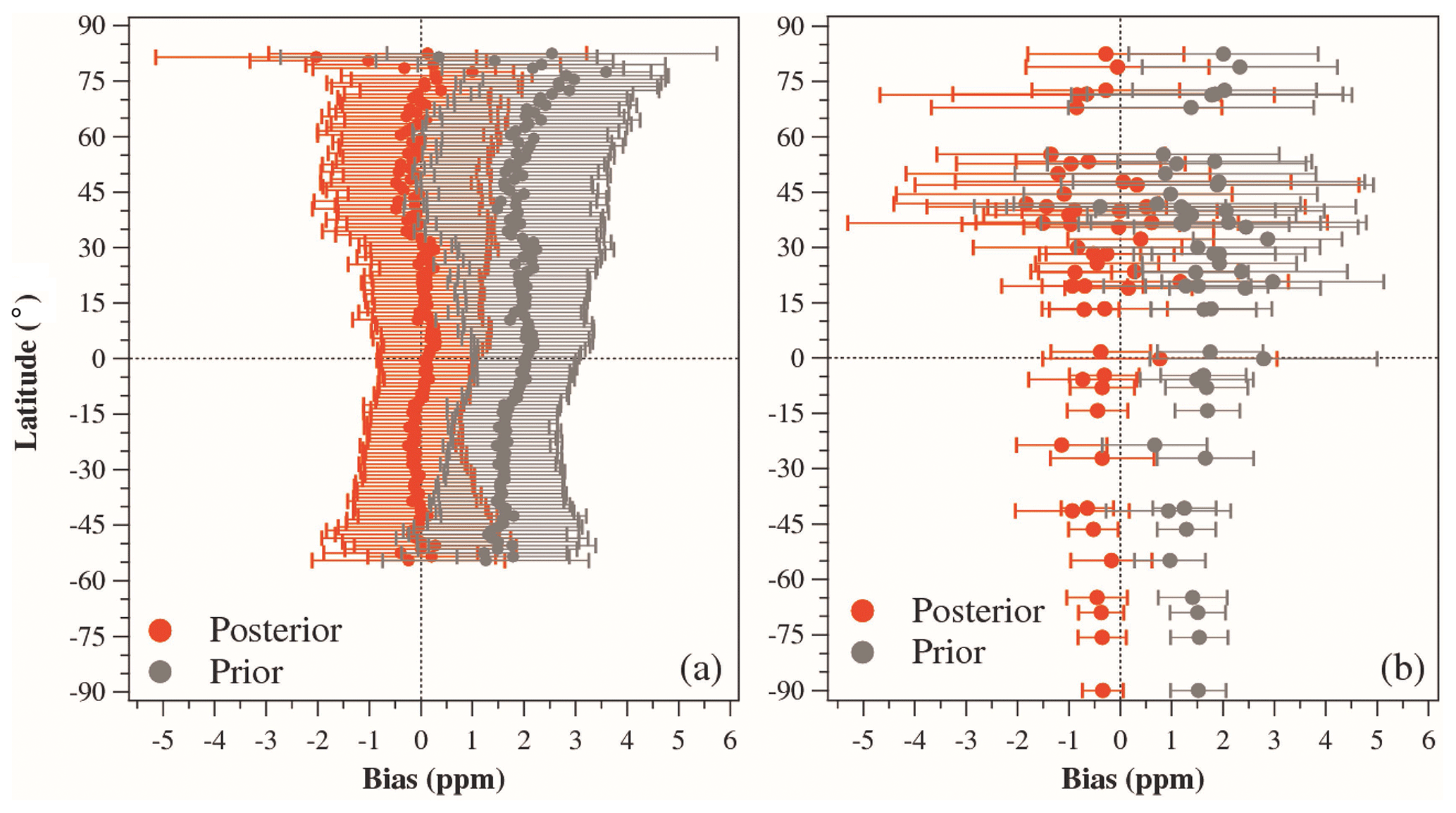
Figure 3 BIAS at different latitudes. Panel a shows the BIAS between the simulated and retrieved XCO₂, and panel b shows the ones between the simulated and observed CO₂ mixing ratios. Error bars represents the standard deviations of the biases at each latitude and each site in panels (a) and (b), respectively.

Table 1 Statistics of the simulated surface CO₂ and XCO₂ concentrations against the surface flask observations and GOSAT retrievals, respectively.

^* Mean ± standard deviation.

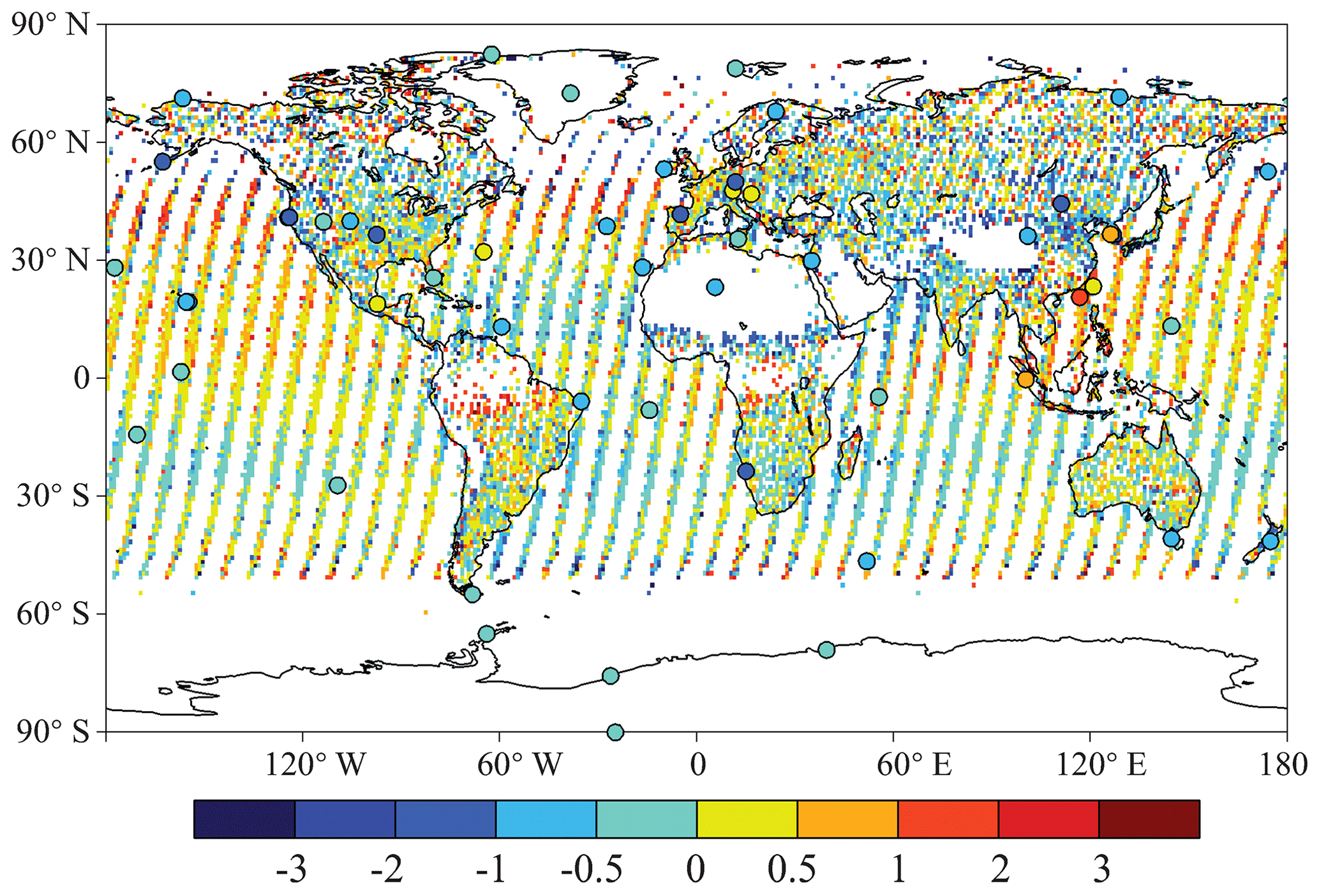
Figure 4 Distributions of the BIAS of the posterior (cycles) surface CO₂ and (shading) XCO₂ concentrations (simulations minus observations or retrievals).

4.1.2 Evaluation using independent surface observations

Figure 3b shows the mean biases of the simulated surface CO₂ mixing ratios at each flask site at different latitudes. It could be found that the BIAS values of the prior CO₂ mixing ratios are basically greater than 1 ppm at different latitudes, with a global mean of 1.6 ± 1.8 ppm; after constraint with the GOSAT XCO₂ retrievals, the BIAS values at most sites are within ± 1 ppm, with a global mean of −0.5 ± 1.8 ppm. These BIAS values are similar to those of Basu et al. (2013), in which the average model–observation bias decreased from a prior value of 1.95 ppm to −0.55 ppm. The MAE and RMSE between the simulated and surface flask concentrations are also decreased at most sites, with the global mean MAE and RMSE decreasing from 2.1 and 2.4 ppm to 1.4 and 1.9 ppm, respectively (Table 1). The BIAS values in the Northern Hemisphere are significantly larger than those in Southern Hemisphere, because the carbon flux in the Northern Hemisphere is more complex than that in the Southern Hemisphere (Wang et al., 2019). In addition, the posterior BIAS values at most sites are negative, especially at midlatitudes in the Northern Hemisphere. The significant negative biases (less than 1 ppm) are mainly distributed in North America, Europe, and central Asia, whereas positive biases are mainly located along the east Asian coast (Fig. 4), indicating that the carbon sinks in North America and Europe might be overestimated in this study, whereas those in the upwind areas of east Asian coastal sites, mainly eastern China, may be underestimated.

Moreover, it also could be found that the global mean prior BIAS of XCO₂ (about 1.8 ppm) is greater than the surface concentrations (1.6 ppm), whereas the BIAS of XCO₂ reduced by inversion (about 1.8 ppm) is less than the reduction in BIAS in the surface concentrations (about 2.1 ppm). This may be attributed to the fact that, on the one hand, although the GOSAT XCO₂ retrievals were bias corrected, there may still be some systematic deviations; on the other hand, the responses of surface observations to changes in the surface carbon flux is faster than the XCO₂ concentrations, so that larger flux adjustments are needed to match the XCO₂ concentration with ground data. A similar situation was reported in Wang et al. (2019). In their study, GOSAT XCO₂ retrievals were used to optimize the terrestrial carbon flux in 2015. Their inversion reduced the BIAS of simulated surface and XCO₂ (compared against TCCON sites) concentrations by about 1.1 ppm and 0.9 ppm, respectively.

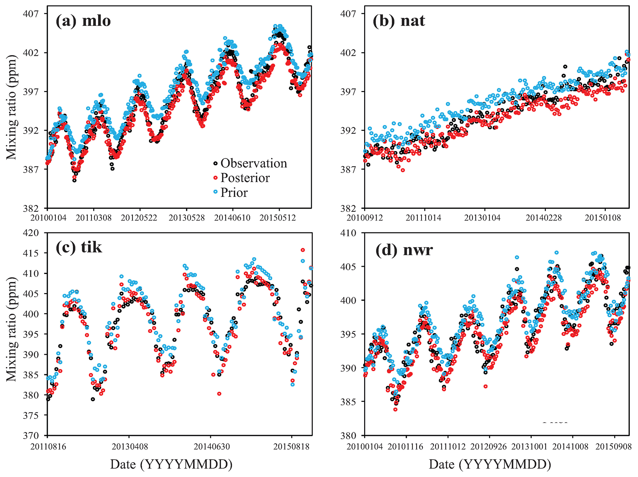
Figure 5 shows the time series of simulated and observed CO₂ mixing ratios at four sites: mlo, nwr, tik, and nat. The mlo and nwr sites are two mountain stations located in the center of the Pacific and western US, respectively, and nat and tik are two coastal sites located in the Amazon and Siberia, respectively (Fig. 2). Overall, the posterior mixing ratios have a better agreement with the observations at all four sites. The mlo site is an atmospheric baseline station. At mlo, the posterior mixing ratio effectively reproduces the observed concentration, whereas the prior concentrations have been overestimated at this site since the summer of 2010, especially during the summertime every year. Moreover, the posterior concentrations during the wintertime are underestimated, and the underestimation gradually increases with time. A similar situation also could be found at the nat site as well as other sites located in the tropical and Southern Hemisphere oceans (not shown). Figure S1 shows the interannual variations in the global mean BIAS. Clearly, the biases of surface CO₂ gradually accumulate, leading to the relatively large mean bias (−0.5 ppm). If we remove the impact of accumulation, the annual BIAS is about −0.1 ppm yr⁻¹ (about −0.2 PgC yr⁻¹). There are no error accumulations at most land sites, such as nwr and tik. These sites indicate that the global net carbon sinks are slightly overestimated every year, but in different lands, there are interannual variations.

Figure 5 Modeled and observed CO₂ time series at four surface stations.

4.2 Uncertainty reduction

The uncertainty reduction (UR) rate is another important quantity to evaluate the performance of GCASv2 and the effectiveness of GOSAT XCO₂ retrievals in this system (Chevallier et al., 2007; Takagi et al., 2011). Following Chevallier et al. (2007), the UR is defined as

$$\begin{array}{}\text{(19)}& \mathrm{UR}=\left(\mathrm{1}-{\displaystyle \frac{{\mathit{\sigma }}_{\mathrm{posterior}}}{{\mathit{\sigma }}_{\mathrm{prior}}}}\right)\times \mathrm{100},\end{array}$$

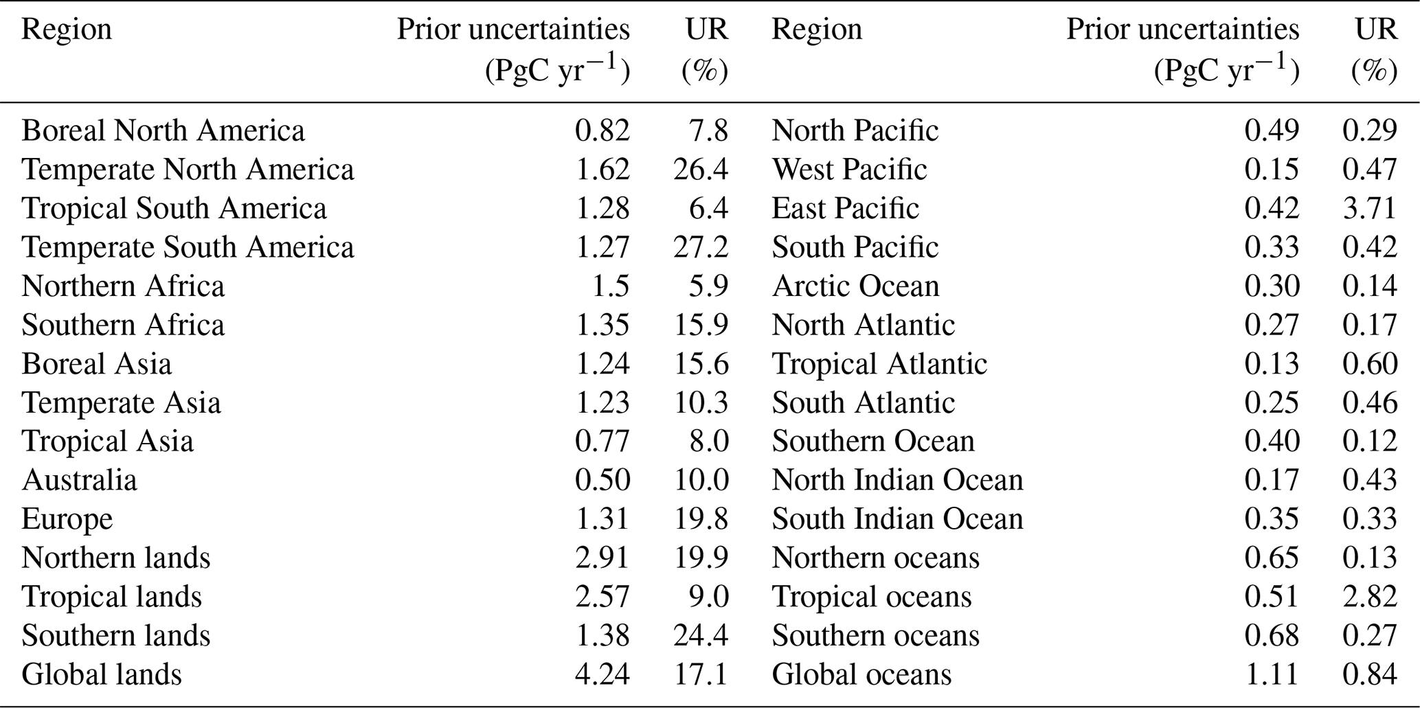
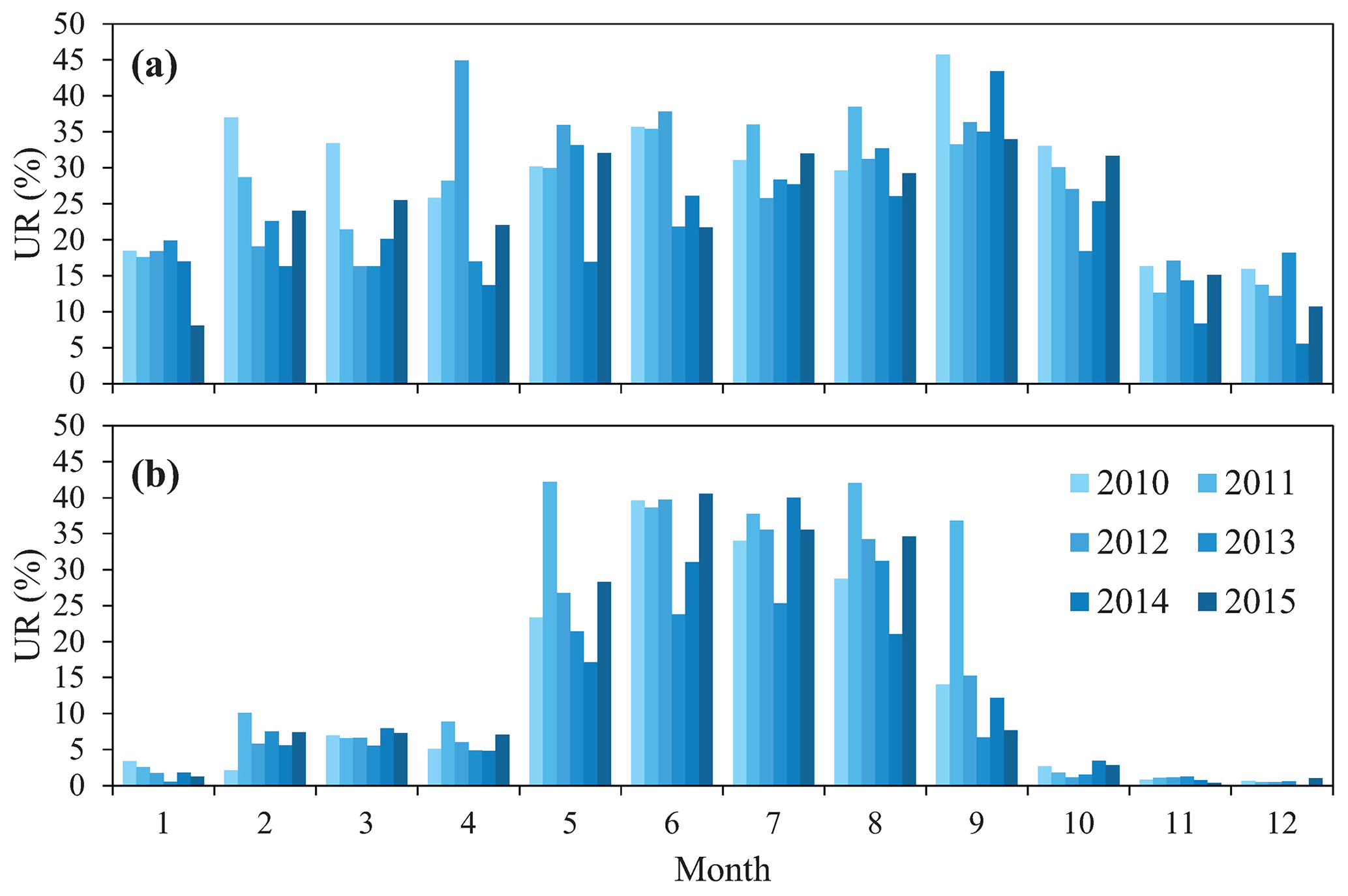
where σ_posterior and σ_prior are the posterior and prior uncertainties, respectively. The URs on regional carbon flux estimates vary significantly over time and space (Deng et al., 2014; Takagi et al., 2011). Table 2 lists the annual mean 1σ URs relative to the prior uncertainties during the 2010–2015 period, which were aggregated in the 22 TransCom regions and 4 large-scale regions. It shows that the annual mean URs are in the range of 6 %–27 % over land regions. The regions with large URs are temperate South America, southern Africa, temperate North America, and Europe. The URs over tropical and boreal regions are relatively small due to the lower spatial coverage of XCO₂. This distribution is similar to the results of Deng et al. (2014), which are mainly related to the spatial coverage of GOSAT XCO₂. Regarding the monthly URs, there are high URs in the warm season and very low URs in cold seasons at high latitudes, the UR is significant throughout the year at midlatitudes, and it is related to the rainy season in tropical areas. In the rainy season, the URs are very low due to the massive cloud coverage, whereas in the dry season, the monthly URs are significant, with the highest UR reaching 25 %. Figure 6 shows the monthly uncertainties in temperate North America and Europe. In Europe, high URs are mainly noted during May–September, and there are high URs in each month in temperate North America, with the highest UR reaching 45 %. The highest monthly UR is in temperate South America, with a value of 50 %. The highest monthly and annual URs are lower than those given in previous studies (40 %–70 %; Takagi et al., 2011; Deng et al., 2014; Saeki et al., 2013a), which may be related to the grided state vector and shorter DA window used in this study.

Over the ocean regions, the URs are very low, with values in the range of 0.12 %–3.7 %. As shown in Formula (14), the UR is mainly determined by the observational uncertainty R and background error covariance P^b (prior uncertainty). Usually, a small R and large P^b correspond to a large UR and vice versa. As we used a scheme in which the prior uncertainties were proportional to the prior fluxes, the regions with small prior fluxes would have small prior uncertainties and small URs. Compared with those over the lands, there are much weaker fluxes and much larger XCO₂ uncertainties (Wunch et al., 2017) over the oceans, resulting in significantly lower URs over the oceans. Previous studies (e.g., Takagi et al., 2011; Kadygrov et al., 2009) have also shown very low URs over the oceans.

Table 2 Annual mean prior uncertainties and reduction rates (UR) aggregated in different TransCom regions during the 2010–2015 period.

Figure 6 Monthly uncertainties in (a) temperate North America and (b) Europe.

4.3 Global carbon budget

Table 3 presents the mean prior and posterior global carbon budgets during the 2010–2015 period of this study. For comparison, the mean global carbon budgets from Global Carbon Budget 2018 (GCP2018; Le Quéré et al., 2018), CT2017, and Jena CarboScope (JCS; Rödenbeck, 2005) are also shown. Both CT2017 and JCS estimates of the surface–atmosphere CO₂ exchange were based on the atmospheric measurements of CO₂ concentrations. In this study, the JCS product of s04oc_v4.3 is adopted. It should to be noted that JCS only provides the net biosphere exchange (NBE), which is the sum of BIO carbon flux and FIRE carbon emissions, and no individual FIRE carbon emissions data are available. For comparison, the FIRE carbon emissions used in this study, which is from CT2017, is also applied to the JCS data, namely the BIO carbon flux of JCS in this paper is obtained from the NBE of JCS minus the FIRE carbon emission of this study.

Table 3 Mean global carbon budgets during the 2010–2015 period estimated in this study as well as those from the prior fluxes, GCP2018, CT2017, and JCS (PgC yr⁻¹).

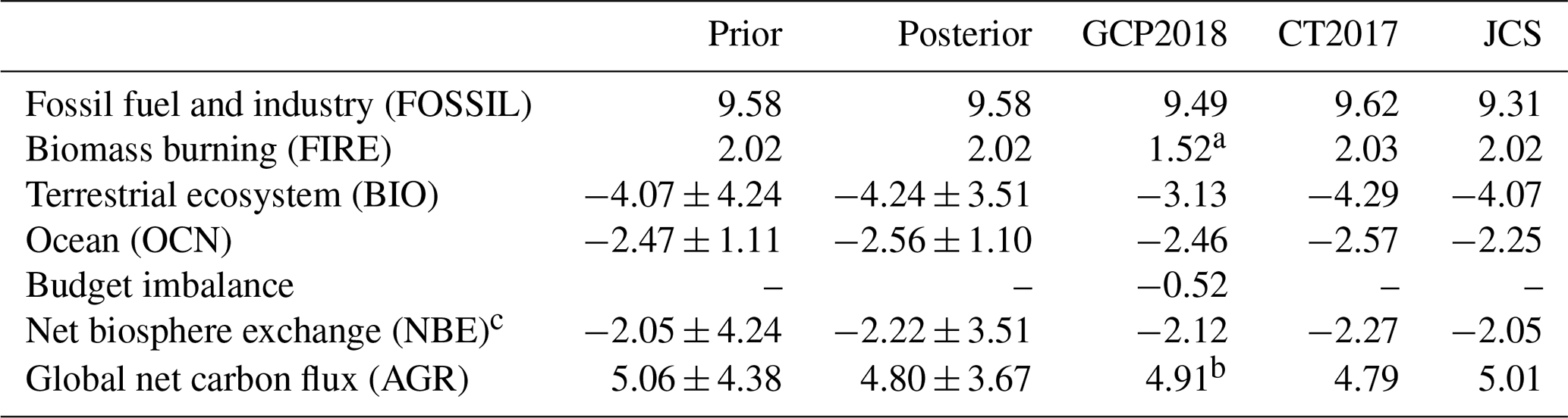
^a Land use change emissions. ^b Atmospheric growth in GCP2018. ^c For GCP2018, it is the sum of BIO, FIRE, and budget imbalance, and for the others, it is the sum of BIO flux and FIRE emissions.

The mean posterior BIO carbon flux during the 2010–2015 period in this study is −4.24 ± 3.51 PgC yr⁻¹ (negative or positive mean carbon uptake or release from or to the atmosphere, same thereafter), and the OCN flux is −2.56 ± 1.10 PgC yr⁻¹; after considering the FOSSIL carbon emission (9.58 PgC yr⁻¹) and FIRE carbon emission (2.02 PgC yr⁻¹), the mean global net carbon flux (i.e., AGR) inverted in this study is 4.80 ± 3.67 PgC yr⁻¹. Both the posterior BIO and OCN carbon fluxes are stronger than the prior fluxes, and the posterior global net carbon flux is weaker than the prior fluxes. Compared with the others, both posterior BIO and OCN fluxes are close to the values of CT2017, but higher than the values of JCS. The AGR of GCP2018 was estimated directly from atmospheric CO₂ measurements, which were provided by the NOAA Earth System Research Laboratory (ESRL) (Dlugokencky and Tans, 2018); therefore, it could be considered as a true value. The posterior AGR in this study (4.8 PgC yr⁻¹) is slightly lower than GCP2018 and very close to CT2017. Compared with GCP2018, the deviations of prior and JCS AGR are 0.15 and 0.10 PgC yr⁻¹, whereas those of posterior and CT2017 are −0.11 and −0.12 PgC yr⁻¹, respectively.

4.4 Regional carbon flux

Figure 7 shows the distributions of the mean prior and posterior annual BIO and OCN carbon fluxes as well as their differences during the 2010–2015 period. For the prior BIO flux, carbon uptakes mainly occur over eastern North America, the Amazon, southern Brazil, western Europe, southern Russia, eastern China, South Asia, and the Malay Archipelago; and carbon releases mainly occur in western North America, the eastern Amazon, Argentina, most of Africa, the former Indochinese Peninsula, and parts of eastern Europe and Russia. For the prior OCN flux, carbon uptakes mainly occur in midlatitude regions in both hemispheres, whereas carbon sources are mainly in tropical oceans and the Southern Ocean. After constraint with the GOSAT XCO₂ retrievals, the overall patterns of carbon sinks and sources are similar to the prior patterns. However, the BIO sinks in eastern and central North America, the eastern Amazon, tropical Africa, the former Indochinese Peninsula, and southwestern Russia are obviously increased; on the contrary, in western North America, temperate South America, extra-tropical Africa, South Asia, southwestern China, North China, Siberia, and parts of southern and northern Europe, the carbon sources are increased. For the OCN flux, in most tropical and Northern Hemisphere oceans, the carbon sinks are slightly increased, whereas the carbon sources are slightly enhanced in most Southern Hemisphere oceans.

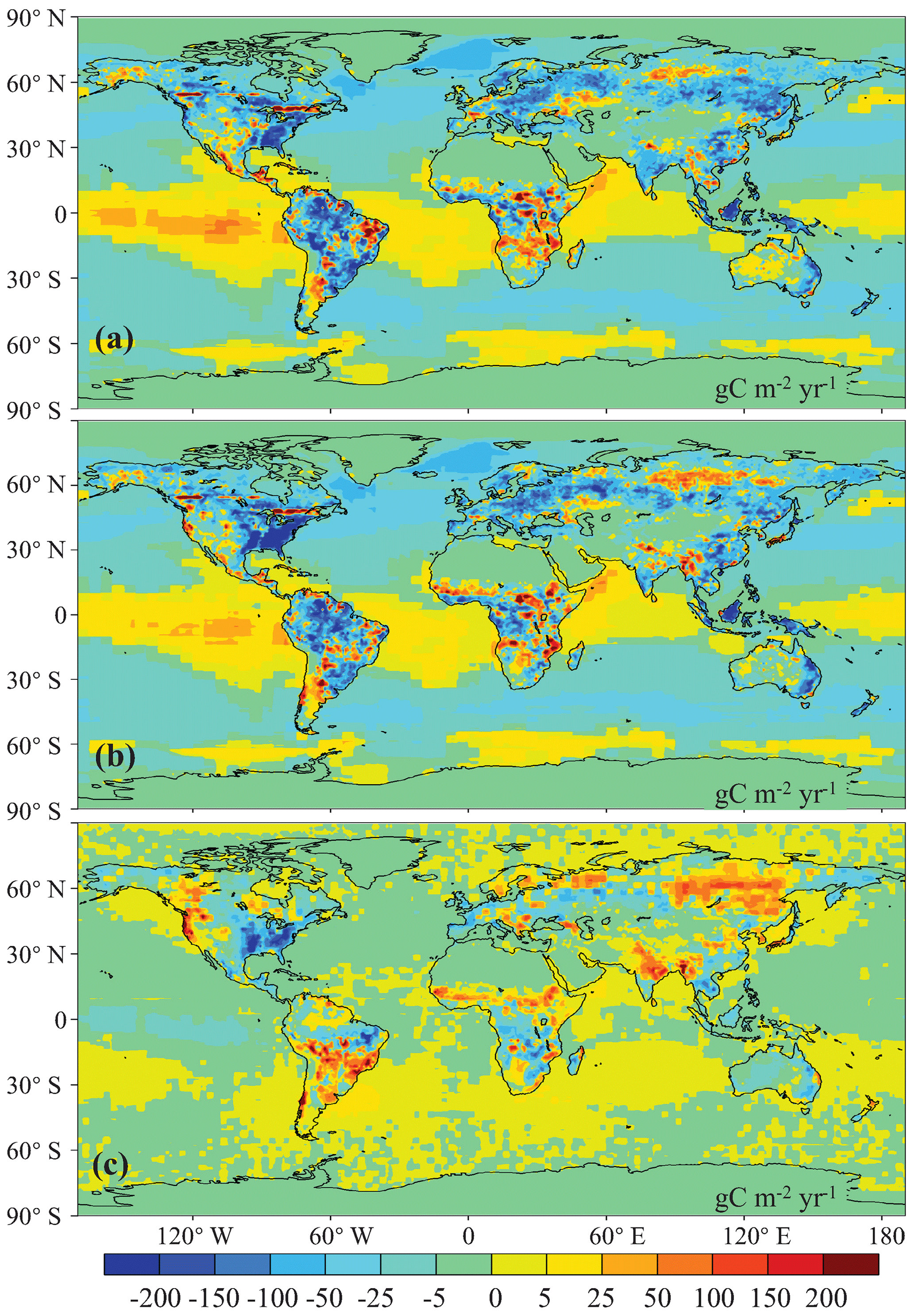
Figure 7 Distributions of the mean annual terrestrial ecosystem and ocean carbon fluxes: (a) prior, (b) posterior, and (c) their differences (posterior–prior) (unit: gC m⁻² yr⁻¹).

Table 4 lists the aggregated mean annual prior and posterior BIO carbon fluxes during the 2010–2015 period for the 11 TransCom land regions (Fig. 2; Gurney et al., 2002) as well as three aggregated large-scale regions, i.e., northern lands, tropical lands, and southern lands. Northern lands include boreal North America, temperate North America, boreal Asia, temperate Asia, and Europe; tropical lands include tropical South America, tropical Asia, northern Africa, and southern Africa; and southern lands include temperate South America and Australia. For the prior, the largest carbon sink is in tropical South America, followed by boreal Asia and temperate Asia, and the weakest carbon flux is in southern Africa. After optimization using GOSAT XCO₂ retrievals, the carbon sinks of temperate North America and southern Africa are significantly increased and those in Australia and Europe are also enhanced. However, in temperate South America, northern Africa, boreal Asia, and temperate Asia, the carbon sinks are decreased. Very small changes are found in boreal North America, tropical South America, and tropical Asia, especially for tropical South America. However, as shown in Fig. 7, there are obvious changes over different areas in tropical South America; thus, the zero change in statistics in this region may just be a coincidence. For the Amazon region (Fig. 2), the estimated BIO flux is decreased from a prior of −0.52 ± 1.46 to −0.45 ± 1.28 PgC yr⁻¹. The largest carbon sink occurs in temperate North America, followed by tropical South America and Europe, and the weakest sink appears in northern Africa.

Table 4 Regional BIO and FIRE flux in the 11 TransCom land regions (PgC yr⁻¹).

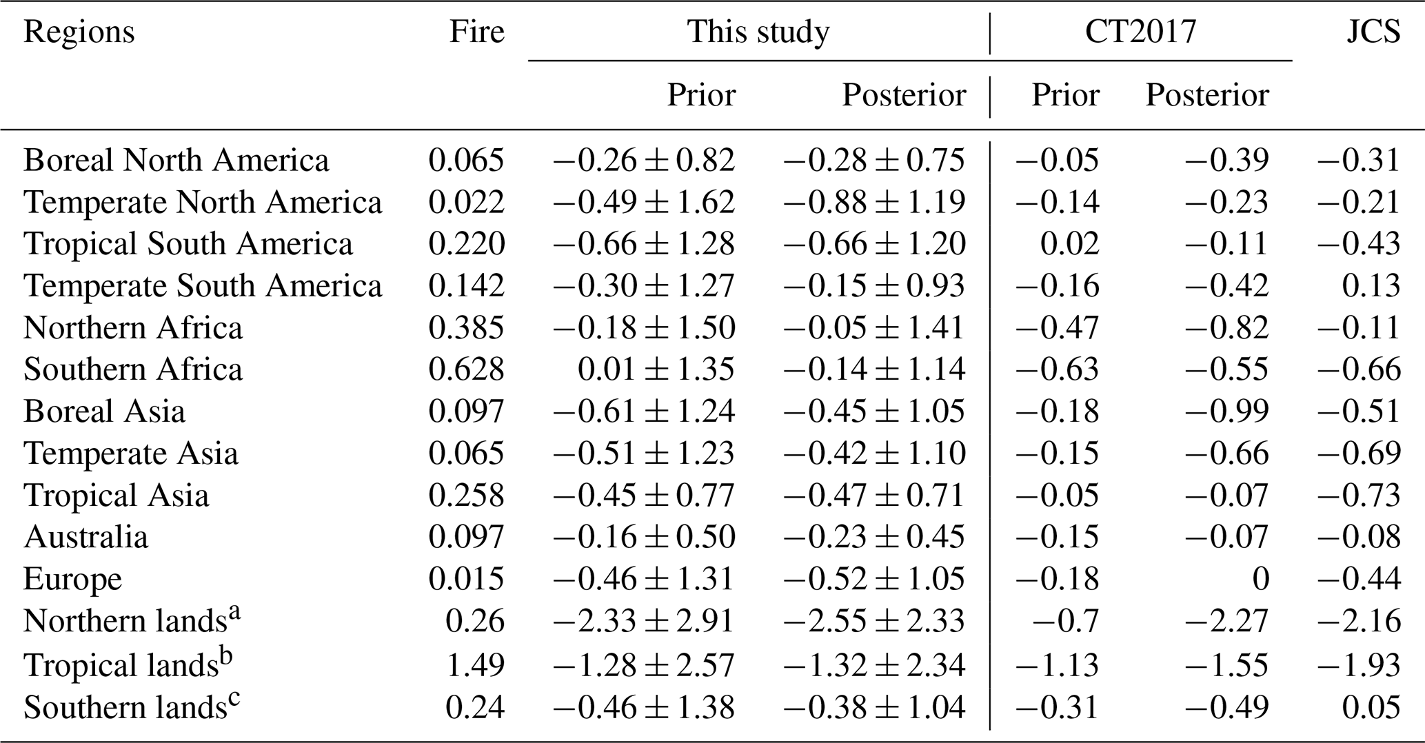
^a Northern lands include boreal North America, temperate North America, boreal Asia, temperate Asia, and Europe. ^b Tropical lands include tropical South America, tropical Asia, northern Africa, and southern Africa. ^c Southern lands include temperate South America and Australia.

For comparison, Table 4 also lists the mean BIO carbon fluxes of CT2017 and JCS for the same period. For the three large-scale regions, i.e., northern lands, tropical lands, and southern lands, their carbon sinks from this study are also similar to CT2017. However, in each region, the distributions of carbon sinks between this study and CT2017 are significantly different. In the northern lands, the carbon sinks estimated by this study are more evenly distributed, although temperate North America has the largest carbon sink, and those in boreal Asia, temperate Asia, and Europe are also very strong and comparable. However, in CT2017, the carbon sinks are mainly distributed in boreal Asia and temperate Asia, accounting for more than 70 % of the total sink in the northern lands. The sinks in temperate North America and Europe are very weak or even neutral. In tropical lands, this study shows strong carbon sinks in tropical South America and tropical Asia as well as a weak sink in Africa, whereas CT2017 shows the opposite pattern. In southern lands, this study shows comparable sinks in temperate South America and Australia, whereas CT2017 shows a strong sink in temperate South America and very weak one in Australia. Compared with JCS, except for temperate North America and southern Africa, the carbon sinks are comparable in other regions. Using different observations as constraints might be one of the main reasons for differences among these studies. Many studies have shown differences between the constraints with in situ observations and XCO₂ retrievals (e.g., Wang et al., 2019; Deng et al., 2014). Furthermore, these differences may be also related to the different prior BIO carbon fluxes among these studies, especially for the tropical land. The distribution of the posterior BIO fluxes in this study and CT2017 are consistent with the corresponding prior fluxes in the tropical lands (Table 4). Using the same GOSAT XCO₂ retrievals, Deng et al. (2014) adopted a similar prior flux to this study, which was also simulated using the BEPS model but globally neutralized, to infer the land fluxes for 2010. The distributions of Deng et al. (2014) are roughly consistent with this study, whereas Wang et al. (2019) applied the prior flux from CT2016 to optimize the fluxes for 2015 and showed a similar distribution of land sinks over the tropical lands to that of CT2017.

Compared with other studies, the land fluxes (including FIRE but excluding FOSSIL) in South America (−0.45 ± 1.51 PgC yr⁻¹), Europe (−0.51 ± 1.05 PgC yr⁻¹), boreal Asia (−0.35 ± 1.05 PgC yr⁻¹), temperate Asia (−0.35 ± 1.10 PgC yr⁻¹), tropical Asia (−0.21 ± 0.71 PgC yr⁻¹), and Australia (−0.13 ± 0.45 PgC yr⁻¹) are comparable with the forest sinks in these regions during the 2000–2007 period estimated using forest inventory data by Pan et al. (2011). However, the land fluxes in Africa and North America are significantly different from the estimates of Pan et al. (2011). In North America, based on inventory-based calculations, the Second State of the Carbon Cycle Report (SOCCR2; Hayes et al., 2018) estimated that the average annual net land ecosystem flux was −0.96 PgC yr⁻¹; after considering the outgassing and wood product emissions, they reported that the land-based carbon sink was −0.606 PgC yr⁻¹ (± 75 %) during the 2004–2013 time period. The land flux estimated in this study (−1.07 PgC yr⁻¹) is close to the bottom-up estimate of the net land ecosystem flux, but it is much stronger than the reported land-based carbon sink of SOCCR2. In Africa, Ciais et al. (2011) showed a comprehensive estimate for its carbon balance, given a sink of −0.2 PgC yr⁻¹ (excluding land use change emissions) based upon observations. Our estimate of the BIO flux in Africa is very consistent with this result. Moreover, most recently, Palmer et al. (2019) inferred the carbon fluxes of pantropical lands in 2015 and 2016 using both GOSAT and the NASA OCO-2 XCO₂ retrievals and showed that net carbon emissions from the African biosphere dominate pantropical atmospheric CO₂ signals, which are similar to the results of this study. In boreal Asia, the land sink estimated by bottom-up approaches was in the range of −0.11 to −0.76 PgC yr⁻¹ (Hayes et al., 2011; Nilsson et al., 2003; Dolman et al., 2012; Zamolodchikov et al., 2017). CT usually reports a very strong carbon sink (Jacobson et al. 2020; Peters et al., 2007; Zhang et al., 2014), and one possible reason for this is that there are not enough surface observations in Asia boreal regions. Saeki et al. (2013b) conducted an inversion with a focus on the Siberia region, and they also derived a large sink of −0.56 ± 0.79 PgC yr⁻¹ using the NOAA data alone; however, after adding additional observations in Siberia, they obtained a weaker uptake of −0.35 ± 0.61 PgC yr⁻¹. Our estimate (−0.35 ± 1.05 PgC yr⁻¹) is in the range of bottom-up estimates and is very consistent with the inversion focused on Siberia (Saeki et al., 2013b). In Europe, previous GOSAT-based inversions consistently derived a very large European sink, which was in the range of −0.6 to −1.8 PgC yr⁻¹(Basu et al., 2013; Chevallier et al., 2014; Deng et al., 2014), whereas those constrained using surface observations were much weaker, in the range of 0 to −0.4 PgC yr⁻¹ (Peters et al., 2007, 2010; Peylin et al., 2013; Scholze et al., 2019). Our estimate of the BIO flux in Europe is smaller than the previous GOSAT-based inversions and is close to the estimate of Pelylin et al. (2013). In the Amazon region, the posterior land flux is −0.45 ± 1.28 PgC yr⁻¹, which is in the range of the previous long-term forest biomass sink estimates of −0.28 to −0.49 PgC yr⁻¹ (Phillips et al., 2009; Brienen et al., 2015) but is larger than the other inversions (e.g., Deng et al., 2016; Gatti et al., 2014).

4.5 Interannual variations

4.5.1 Global land and ocean fluxes

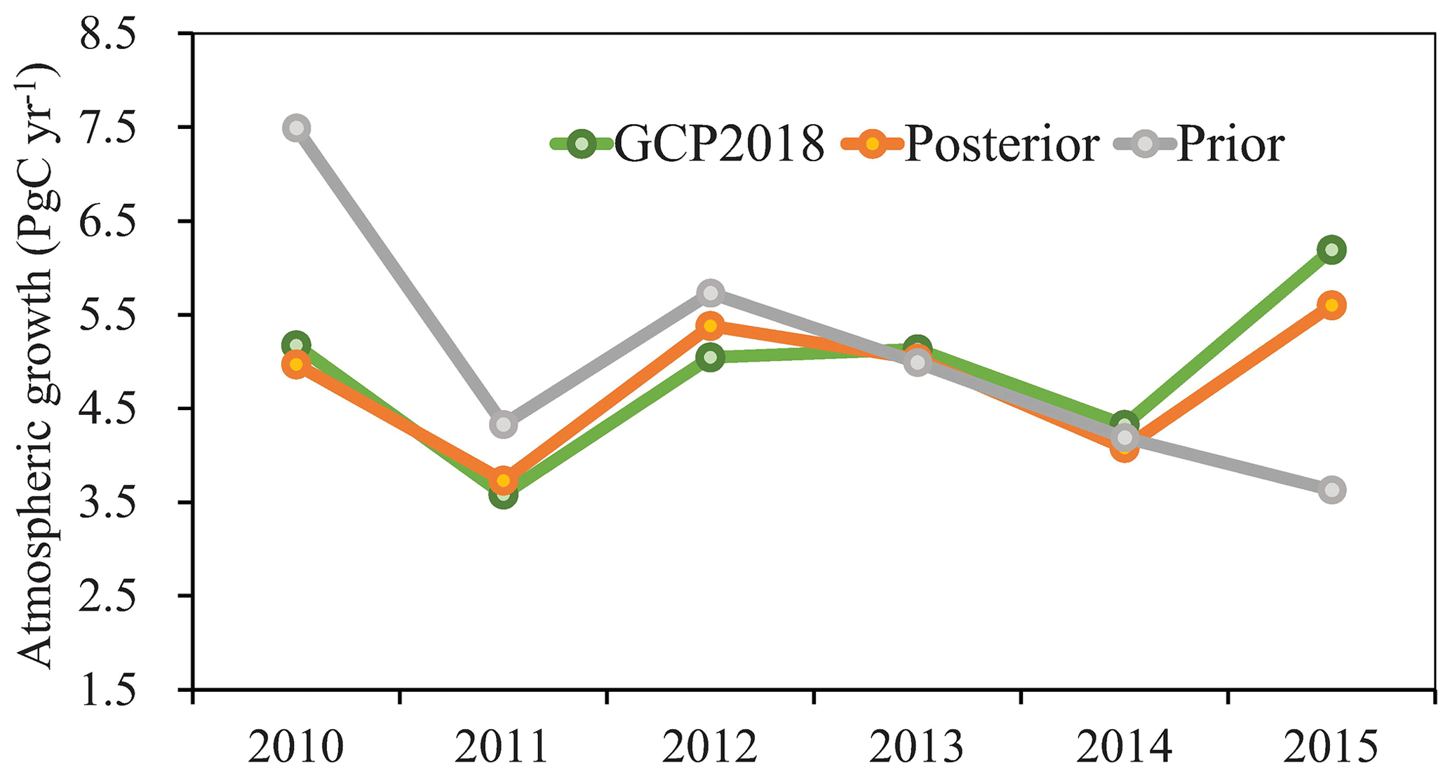
Figure 8 shows the interannual variations in the prior and posterior BIO and OCN fluxes. Overall, from 2010 to 2015, the prior BIO fluxes show an increasing trend, but for the posterior fluxes, there is no significant trend. Large differences between the prior and posterior fluxes mainly occur in 2010 and 2015. In 2010, the posterior sink is much stronger than the prior, whereas the posterior sink is much weaker than the prior in 2015. For the OCN flux, both prior and posterior fluxes show consistently upward trends, and the posterior sinks are basically stronger than the prior ones every year except for 2015. For the AGR (Fig. 9), the prior value shows a significant downward trend, whereas the posterior value shows a slightly increasing trend. As for the BIO fluxes, large differences mainly occur in 2010 and 2015.

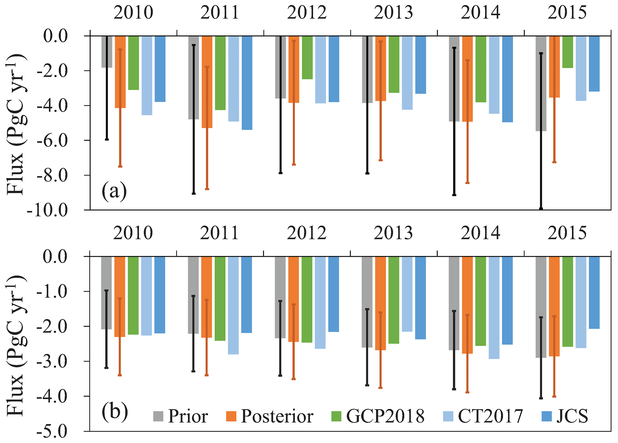
Figure 8 Interannual variations in global (a) BIO and (b) OCN fluxes of the prior and posterior as well as GCP2018, CT2017, and Jena CarboScope (JCS).

Compared with the other products, the interannual variations in the posterior BIO fluxes (Fig. 8a) are consistent with the inversions of CT2017 and JCS as well as the estimates of GCP2018. For each year, the inversions of this study are within the range of CT2017 and JCS, but they are higher than GCP2018. However, because GCP2018 has the budget imbalance item and the land use change emission is different from the FIRE emission, the BIO flux in GCP2018 is different from this study; therefore, direct comparison with GCP2018 is not meaningful. For OCN fluxes, overall, there are no significant differences among different estimates, and the upward trend of this study is similar to that of GCP2018 and higher than those of CT2017 and JCS. The interannual variation in AGR in this study is also very consistent with GCP2018 (Fig. 9). Except for 2012 and 2015, the absolute deviations of AGR between this study and GCP2018 are within 0.3 PgC yr⁻¹.

Figure 9 Interannual variations in the atmospheric CO₂ growth rates.

4.5.2 Regional land fluxes

Figure 10a, b, and c show the prior and posterior interannual variations in the BIO fluxes in the northern lands, tropical lands, and southern lands, respectively. In the northern lands, the interannual variations in both prior and posterior fluxes are similar to the corresponding global land totals (Fig. 8a), i.e., upward trend for the prior flux and no trend with the posterior flux, indicating that the interannual variations in global BIO fluxes are dominated by the fluxes in the northern lands. In the tropical lands, the interannual variations in posterior fluxes are similar to the prior fluxes; however, compared with the prior sinks in 2010 and 2011, the posterior sinks are much stronger, whereas in 2013 and 2015, they are much weaker. In the southern lands, there are large differences in the interannual variations between the prior and posterior fluxes. For the prior flux, the highest sink is in 2011 and the weakest is in 2012; after 2012, the prior flux sink increases year by year, whereas the posterior flux sink decreases from 2010 to 2013 and then increases thereafter.

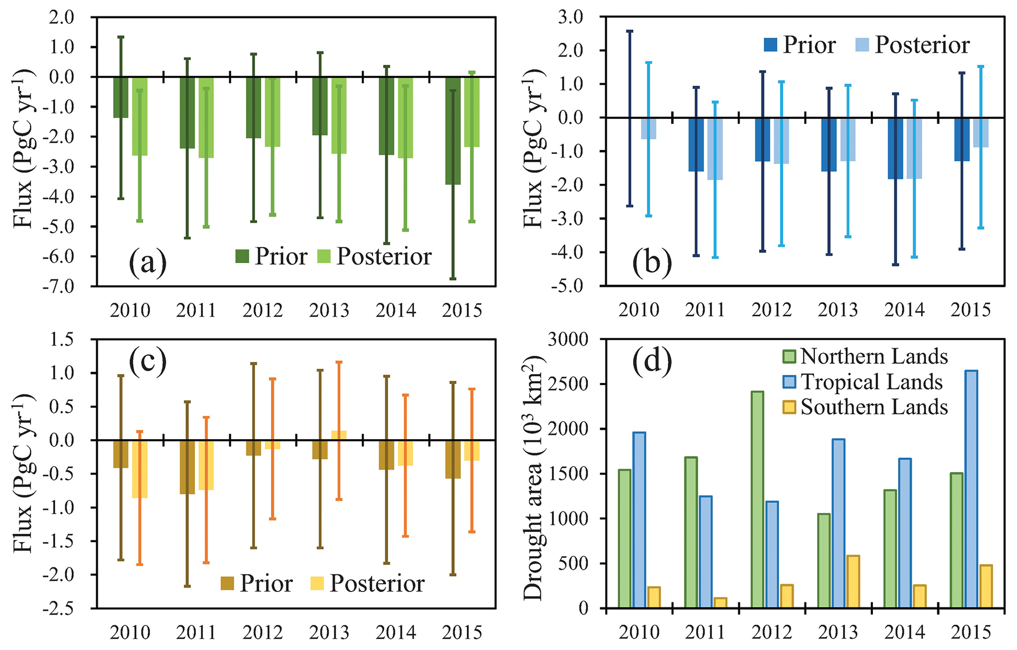
Figure 10 Prior and posterior interannual variations in the BIO fluxes in the (a) northern lands, (b) tropical lands, and (c) southern lands, respectively, and (d) severe drought areas of the abovementioned regions.

Drought is one of the most important factors affecting terrestrial carbon sinks, and severe drought will generally significantly reduce carbon sinks (e.g., Ma et al., 2012; Zhao and Running, 2010; Ciais et al., 2005; Gatti et al., 2014; Phillips et al., 2009; Vicente-Serrano et al., 2013). Previous studies (e.g., Liu et al., 2018) have used the GOSAT XCO₂ retrievals to infer the impact of droughts on terrestrial ecosystem carbon uptake anomalies. Figure 10d shows the severe drought areas (SDAs) in the three large-scale regions every year, which were calculated according to the monthly standardized precipitation–evapotranspiration index at 12-month timescales (SPEI12; Beguería et al., 2010). Here, the SPEIbase v2.5 database is used, and severe drought is defined as an SPEI12 less than −1.5 (Paulo et al., 2012). In addition, only severe droughts that occur in forests, shrubs, and crops are considered in this study. It was found that the posterior fluxes have better correlations with the SDAs in all three regions, i.e., a larger SDA leads to a weaker carbon sink and vice versa. The correlation coefficients between carbon sinks and SDAs in the northern lands, tropical lands, and southern lands increase from prior values of −0.1, −0.25, and −0.44 to −0.53, −0.67, and −0.76, respectively, indicating that the inversion has improved the interannual variations in BIO fluxes at large scales. In addition, a strong El Niño event happened during 2015–2016, and many researchers have studied the responses of tropical land carbon fluxes to this strong event (e.g., Wang et al., 2018b; Liu et al., 2017; Bastos et al., 2018; Koren et al., 2018). Liu et al. (2017) found that, relative to the 2011 La Niña, the pantropical biosphere released 2.5 ± 0.34 PgC more carbon into the atmosphere in 2015. Bastos et al. (2018) showed a smaller difference in carbon fluxes between 2015 and 2011, using both bottom-up and top-down approaches, which was in the range of −0.7 to −1.9 PgC yr⁻¹. In this study, compared with the prior, our inversion significantly enhances the difference between 2011 and 2015 (Fig. 10b) and shows that 2015 released 1.35 PgC more than 2011 in the pantropical region (defined following Liu et al., 2017), which is much lower than the result from Liu et al. (2017) but agrees well with the result of Bastos et al. (2018).

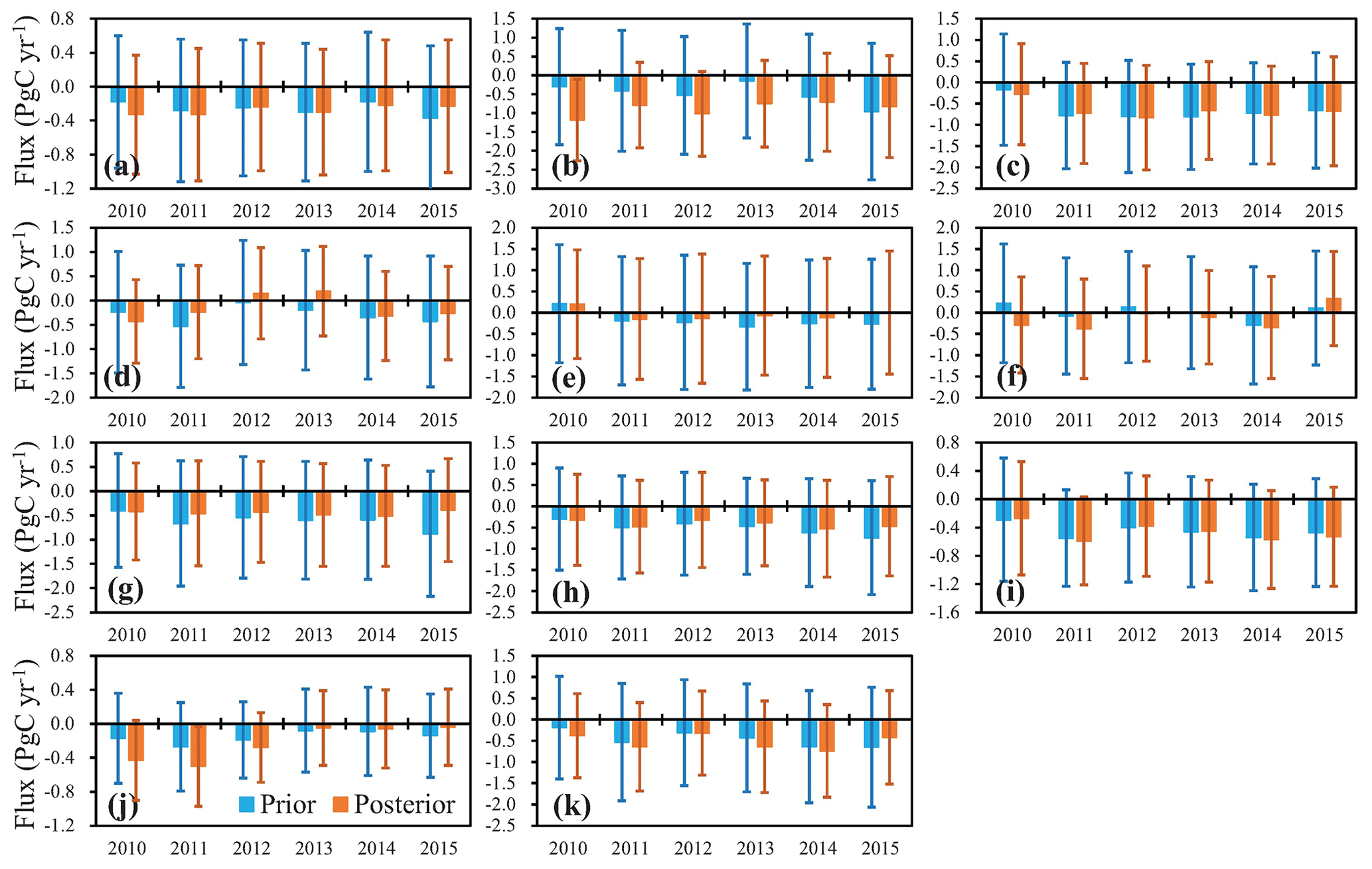
Figure 11 Prior and posterior interannual variations in the BIO fluxes for (a) boreal North America, (b) temperate North America, (c) tropical South America, (d) temperate South America, (e) northern Africa, (f) southern Africa, (g) boreal Asia, (h) temperate Asia, (i) tropical Asia, (j) Australia, and (k) Europe.

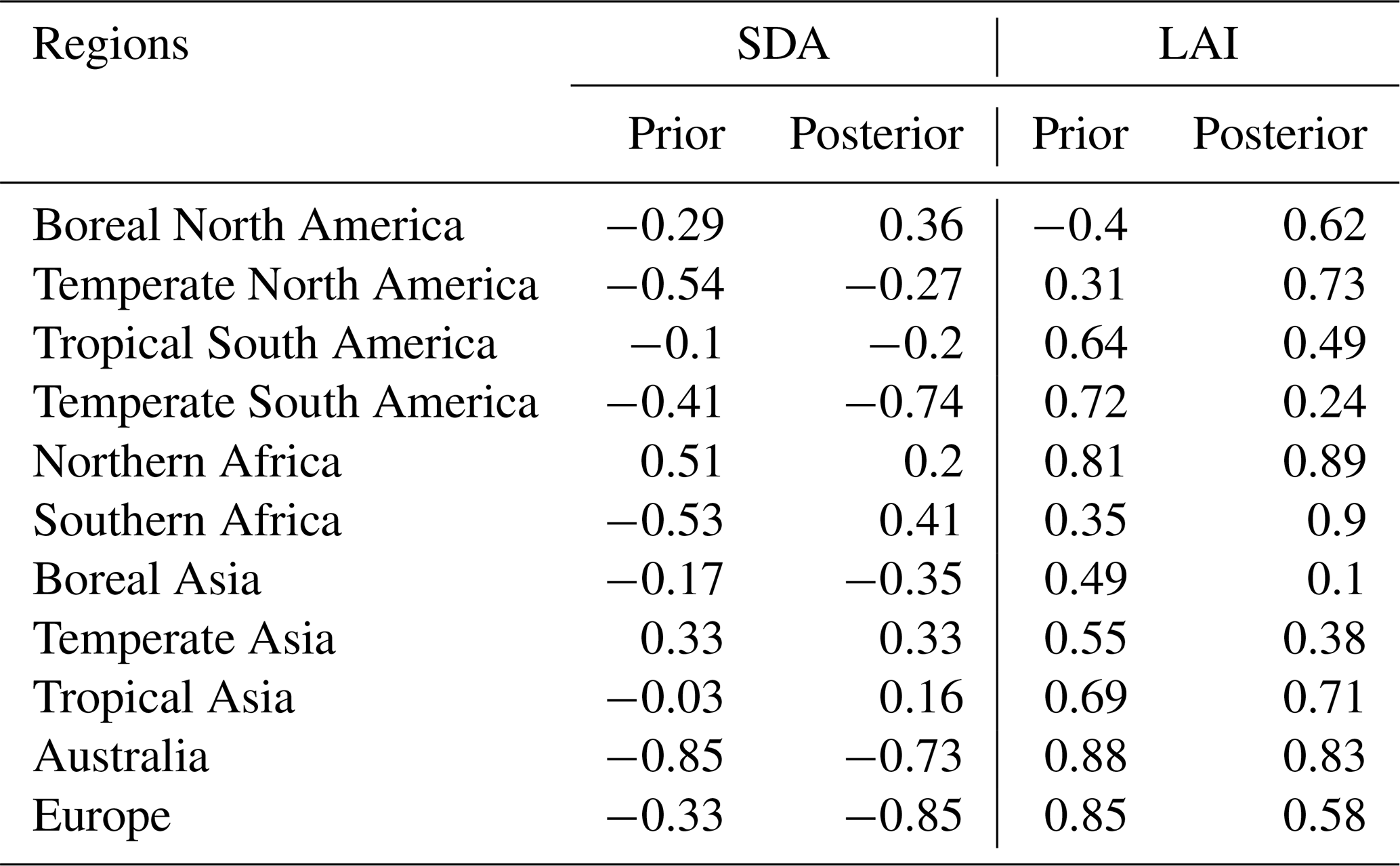
Table 5 Correlation coefficients of severe drought areas (SDAs) and the regional mean LAI with the BIO sinks in each region.

Moreover, Fig. 11 shows the prior and posterior interannual variations in the BIO fluxes for the 11 TransCom land regions. In North America, including temperate North America and boreal North America, the prior fluxes show an upward trend, whereas the posterior fluxes show a downward trend. In boreal Asia and temperate Asia, there are significant upward trends for the prior fluxes, but no significant trends are found in the posterior fluxes. In temperate South America, although the prior and posterior fluxes show trends of weakening first and then increasing, the years in which the carbon sink is weakest are not consistent: the prior flux is weakest in 2012, whereas the posterior flux is weakest in 2013. Similarly, in northern Africa, the prior and posterior fluxes show a trend of increasing and then decreasing, but the prior flux is strongest in 2014, whereas the posterior flux is strongest in 2011. In other regions, such as tropical South America, tropical Asia, southern Africa, Australia, and Europe, the trends between the prior and posterior fluxes are similar, especially in tropical South America and tropical Asia where the prior and posterior fluxes are very close every year. In southern Africa and Australia, the posterior fluxes have more significant interannual variations than the prior fluxes, and in Europe, the posterior sink is much weaker in 2015 and is stronger in 2010 and 2013 than the prior sink.

As above, here we also investigate the relationships between the interannual variations in carbon sinks and SDAs in the 11 TransCom land regions. As shown in Table 5, in temperate South America, boreal Asia, and Europe, the posterior sinks have a better correlation with the SDAs than the prior sinks; specifically, in Europe, the correlation coefficient increases from a prior value of −0.33 to −0.85. However, in other regions, there is no obvious improvement, and in some regions, such as boreal North America, temperate North America, northern Africa, and southern Africa, the relationships even become worse. One possible reason for this is that there are usually higher annual mean temperatures in drought years, which might extend the growing season for vegetation, thereby enhancing the carbon uptake and offsetting the impacts of drought. A previous study by Wolf et al. (2016) showed that temperate North America experienced an extreme summer drought event in 2012, along with the warmest spring on record. They quantified the impact of this climate anomaly on the carbon cycle and concluded that the warm spring largely increased spring carbon uptake and, thus, compensated for reduced carbon uptake induced by the summer drought. Liu et al. (2018) reported that because of the compensating effect of the carbon flux anomalies between the northern and southern US in 2011 and between spring and summer in 2012, the annual carbon uptake decreased by 0.10 ± 0.16 PgC in 2011 and increased by 0.10 ± 0.16 PgC in 2012 over the US compared with the average state. In this study, compared with the mean flux during the 2010–2015 period, the carbon sink in temperate North America decreased by 0.09 PgC yr⁻¹ in 2011 and increased by 0.14 PgC yr⁻¹ in 2012, which is very close to the result of Liu et al. (2018). In Australia, both the prior and posterior fluxes have very good relationships with the SDAs. The significantly enhanced carbon uptake during the 2010–2012 period is consistent with the findings of Detmers et al. (2015), who inferred an even stronger carbon sink of −0.77 ± 0.10 PgC yr⁻¹ from the end of 2010 to early 2012 using the GOSAT XCO₂ product. They also confirmed that this enhanced sink was related to the strong La Niña episode, which brought a record-breaking amount of precipitation, resulting in enhanced vegetation growth. In tropical South America, the impacts of the 2010 drought on the carbon uptake over the Amazon have been extensively studied (e.g., Doughty et al., 2015; Gatti et al., 2014; van der Laan-Luijkx et al., 2015). The year 2010 was a drought year, whereas 2011 was a wet year in the Amazon region. Comparing 2010 with 2011, Gatti et al. (2014) estimated that the no-fire carbon exchange was reduced by 0.22 PgC yr⁻¹, van der Laan-Luijkx et al. (2015) derived a decrease in the biospheric uptake ranging from 0.08 to 0.26 PgC yr⁻¹, and Doughty et al. (2015) concluded that drought suppressed Amazon-wide photosynthesis by 0.23–0.53 PgC yr⁻¹. In this study, our inversion reduces the difference in carbon uptake between 2010 and 2011 from a prior of 0.62 PgC yr⁻¹ to 0.28 PgC yr⁻¹, which is much more consistent with the previous estimates.

Carbon uptake occurs mainly through photosynthesis by vegetation leaves. The LAI is a measure of leaf area per unit area. Buchmann and Schulze (1999) showed that there are strong relationships between the interannual changes in carbon uptake and the LAI in grasslands, C₄ crops, and coniferous forests, but no significant relationship in broad-leaved forests; Chen et al. (2019) also showed that from 1981 to 2016, the increase in the LAI contributed significantly to the increase in global BIO carbon sinks. Therefore, we further investigate the relationships between the interannual changes in carbon sinks and the LAI in the 11 TransCom regions (Table 5). Here, the LAI data are from the Global Inventory Modeling and Mapping Studies (GIMMS) LAI3g product, which has a spatial resolution of $\mathrm{1}/\mathrm{12}$^∘ and a time interval of 15 d (Zhu et al., 2013). As shown in Table 5, in boreal North America, temperate North America, northern Africa, and southern Africa, compared with the prior fluxes, there are better relationships between the posterior carbon sinks and LAIs: the correlation coefficients increase from prior values of −0.4, 0.31, and 0.35 to 0.62, 0.73, and 0.90 respectively, suggesting that the inversion of this study may also improve the interannual variations in carbon sinks in these four regions at a certain extent.

5 Summary and conclusions

In this study, we upgrade the GCAS system to GCASv2 using new assimilation algorithms, procedures, and a localization scheme, as well as higher assimilation parameter resolution and the ability to assimilate XCO₂ retrievals. We then use the GOSAT XCO₂ retrievals to constrain terrestrial ecosystem and ocean carbon fluxes from 1 May 2009 to 31 December 2015, with the GCASv2 system. We compare the simulated prior and posterior XCO₂ against the corresponding GOSAT XCO₂ retrievals to test the effectiveness of the assimilation system and evaluate the posterior carbon fluxes by comparing the posterior CO₂ mixing ratios against observations from 52 surface flask sites. The distribution and interannual variations in the posterior carbon fluxes at both global and regional scales from 2010 to 2015 are shown and discussed.

Compared with the GOSAT XCO₂ retrievals, the global mean BIAS and RMSE decrease from prior values of 1.8 ± 1.3 and 2.2 ppm to −0.0 ± 1.1 and 1.1 ppm, respectively, indicating that the GCASv2 system works well with the GOSAT XCO₂ retrievals. Independent evaluations using surface flask CO₂ concentrations showed that the posterior carbon fluxes could significantly improve the modeling of atmospheric CO₂ concentrations, with the global mean BIAS and RMSE decreasing from prior values of 1.6 ± 1.8 and 2.4 ppm to −0.5 ± 1.8 and 1.9 ppm, respectively. The large negative biases are mainly distributed in North America and Europe, indicating the overestimates of carbon sinks over these areas. Evaluations also show that the biases gradually increase along with time in most tropical and Southern Hemisphere ocean sites, but no accumulation is found at most land sites. This indicates that the carbon sinks may be overestimated every year at the global scale, but in different lands, the deviations of the estimates may differ each year.

Globally, the mean annual BIO carbon sink and the interannual variations inferred in this study are very close to the estimates of CT2017 during the study period, and the estimated mean AGR and interannual changes are also very close to the observations, with a mean annual bias of −0.11 PgC yr⁻¹. Regionally, the inversion shows that in the northern lands, the carbon sink of temperate North America is the strongest, and those in boreal Asia, temperate Asia, and Europe are also very strong and comparable; in the tropics, there are strong sinks in tropical South America and tropical Asia, but a very weak sink in Africa. These distributions are significantly different from the estimates of CT2017, probably due to the different prior fluxes and CO₂ observations used for inversion. However, our estimates in most regions or on most continents are comparable or are in the range of previous bottom-up estimates. The inversion also changed the interannual variations in carbon sinks in most TransCom and hemispheric-scale land regions, leading to their better relationship with the variations in severe drought or LAI and indicating that the inversion with GOSAT XCO₂ retrievals may help to better understand the interannual variations in regional carbon fluxes.