the Creative Commons Attribution 4.0 License.
the Creative Commons Attribution 4.0 License.
 | 22 Dec 2021
The drivers and health risks of unexpected surface ozone enhancements over the Sichuan Basin, China, in 2020
Youwen Sun
Hao Yin
Justus Notholt
Mathias Palm
Cheng Liu
Yuan Tian
Following a continuous increase in the surface ozone (O3) level from 2013 to 2019, the overall summertime O3 concentrations across China showed a significant reduction in 2020. In contrast to this overall reduction in surface O3 across China, unexpected surface O3 enhancements of 10.2 ± 0.8 ppbv (23.4 %) were observed in May–June 2020 (relative to 2019) over the Sichuan Basin (SCB), China. In this study, we use high-resolution nested-grid GEOS-Chem simulation, the eXtreme Gradient Boosting (XGBoost) machine learning method, and the exposure–response relationship to determine the drivers and evaluate the health risks due to the unexpected surface O3 enhancements. We first use the XGBoost machine learning method to correct the GEOS-Chem model–measurement O3 discrepancy over the SCB. The relative contributions of meteorology and anthropogenic emission changes to the unexpected surface O3 enhancements are then quantified with a combination of GEOS-Chem and XGBoost models. In order to assess the health risks caused by the unexpected O3 enhancements over the SCB, total premature mortalities are estimated. The results show that changes in anthropogenic emissions caused a 0.9 ± 0.1 ppbv O3 reduction, whereas changes in meteorology caused an 11.1 ± 0.7 ppbv O3 increase in May–June 2020 relative to 2019. The meteorology-induced surface O3 increase is mainly attributed to an increase in temperature and decreases in precipitation, specific humidity, and cloud fractions over the SCB and surrounding regions in May–June 2020 relative to 2019. These changes in meteorology combined with the complex basin effect enhance biogenic emissions of volatile organic compounds (VOCs) and nitrogen oxides (NOx), speed up O3 chemical production, and inhibit the ventilation of O3 and its precursors; therefore, they account for the surface O3 enhancements over the SCB. The total premature mortality due to the unexpected surface O3 enhancements over the SCB has increased by 89.8 % in May–June 2020 relative to 2019.
- Article
(6786 KB) - Full-text XML
-
Supplement
(2659 KB) - BibTeX
- EndNote


Surface ozone (O3) is largely generated from its local anthropogenic (fossil fuel and biofuel combustions) and natural (biomass burning, BB; lightning; and biogenic emissions) precursors, such as volatile organic compounds (VOCs), nitrogen oxides (NOx), and carbon monoxide (CO), via a chain of photochemical reactions (Cooper, 2019; Sun et al., 2018). An additional portion of surface O3 is transported from distant regions via long-range transport or from the stratosphere (Akimoto et al., 2015; H. Y. Wang et al., 2020). Surface O3 is one of the most harmful air pollutants, and it threatens human health and crop production (Fleming et al., 2018; Lu et al., 2020; Sun et al., 2018; Van Dingenen et al., 2009). Exposure to ambient O3 pollution evokes a series of health risks including stroke, respiratory disease (RD), hypertension, cardiovascular disease (CVD), and chronic obstructive pulmonary disease (COPD) (Brauer et al., 2016; Lelieveld et al., 2013; Li et al., 2015; Liu et al., 2018; Lu et al., 2020; P. Wang et al., 2020). Lu et al. (2020) estimated that the premature RD mortalities attributable to ambient O3 exposure in 69 Chinese cities in 2019 reached up to 64 370.
Surface O3 variability is sensitive to both emissions and meteorological changes (Liu and Wang, 2020a, b; X. Lu et al., 2019a). Meteorological conditions affect surface O3 variability indirectly through changes in the natural emissions of its precursors or directly via changes in wet and dry removal, dilution, chemical reaction rates, and transport flux (Li et al., 2019a; Lin et al., 2008; Liu and Wang, 2020a; X. Lu et al., 2019b). A reduction in temperature can lessen O3 production by slowing down the chemical reaction rates (Fu et al., 2015; Lee et al., 2014; Liu and Wang, 2020a) or reducing the biogenic VOC and NOx emissions (Guenther et al., 2006; Im et al., 2011; Tarvainen et al., 2005). Dryer meteorological conditions can result in an increase in surface-level O3 (He et al., 2017; Kalabokas et al., 2015; Liu and Wang, 2020a). Depending on which process dominates the influence of the planetary boundary layer height (PBLH) on surface pollutants, a higher PBLH can either reduce surface-level O3 by diluting O3 and its precursors into a larger volume of air (Sanchez-Ccoyllo et al., 2006; X. Wang et al., 2020) or increase surface-level O3 by transporting more O3 from the upper troposphere or lessening NO abundance for O3 titration (He et al., 2017; Liu and Wang, 2020a; Sun et al., 2009). Precipitation has been verified to decrease surface-level O3 through the wet removal of its precursors, and clouds reduce surface-level O3 by decreasing the oxidative capacity of the atmosphere and enhancing scavenging of atmospheric oxidants (Lelieveld and Crutzen, 1990; Liu and Wang, 2020b; Shan et al., 2008; Steinfeld, 1998). A higher wind speed can decrease surface-level O3 by fast ventilation of O3 and its precursors (X. Lu et al., 2019a; Sanchez-Ccoyllo et al., 2006).
Emissions of air pollutants affect surface O3 variability by perturbing the abundances of hydroperoxyl (HO2) and alkylperoxyl (RO2) radicals, which are the key atmospheric constituents in formation of O3 (Liu and Wang, 2020b). Many previous studies have verified a non-linear relationship between O3 and its precursors (e.g. Atkinson, 2000; Liu and Wang, 2020b; X. Lu et al., 2019b; Sun et al., 2018; Wang et al., 2017). If surface O3 formation regime lies within the VOC-limited region, reductions in VOC emissions will result in a reduction in surface-level O3. Similarly, if the surface O3 formation regime lies within the NOx-limited region, reductions in NOx emissions will result in a reduction in surface-level O3 (Atkinson, 2000; Wang et al., 2017). If surface O3 formation regime lies within transitional region, reductions in either VOC or NOx emissions will result in a reduction in surface-level O3. Atmospheric aerosols can affect the surface O3 level through either heterogeneous reactions of reactive gases (Li et al., 2018; Lou et al., 2014; Lu et al., 2012; Stadtler et al., 2018) or by affecting the solar radiation for gases' photolysis and oxidation (Li et al., 2011; X. Lu et al., 2019a, b; Xing et al., 2017).
Understanding the drivers of surface O3 variability has strong implications for O3 mitigation (Chen et al., 2020; X. Lu et al., 2019a; Sun et al., 2018). China has experienced a continuous increase in surface-level O3 despite the implementation of NOx control measures since 2013 (Liu and Wang, 2020a, b; Lu et al., 2018, 2020). Many studies have attempted to determine the drivers of high-O3 events that have occurred in specific regions and during specific time periods across China. Most of these studies have focused on the most densely populated and highly industrialized areas in eastern China, whereas studies in the remaining part of the country are still limited (Liu and Wang, 2020a, b; K. D. Lu et al., 2019a, b, 2012; H. C. Wang et al., 2020; Wang and Lu, 2019; Wang et al., 2017). As China has a vast territory with a wide range of emission levels and meteorological conditions, O3 variability and its drivers may vary both temporally and geographically; thus, the results from one region are not likely to be applied nationally. In addition, previous studies typically use state-of-the-art chemical transport models (CTMs) with sensitivity simulations to quantify the drivers of O3 variability, e.g. fixed meteorology but varied emission levels to quantify the influences of emission changes or vice versa (Liu and Wang, 2020a, b; K. D. Lu et al., 2019a). However, uncertainties in local meteorological fields, emission estimates, and model mechanisms can lead to a discrepancy in CTMs that may affect the accuracy of O3 predictions as well as their sensitivities to changes in emissions and meteorology (X. Lu et al., 2019a; Young et al., 2018). This is particularly relevant for the Sichuan Basin (SCB), one of the most industrialized and populated city clusters in western China, where large discrepancies between measured and modelled surface O3 are found due to the complex terrain (X. Lu et al., 2019a; X. Wang et al., 2020).
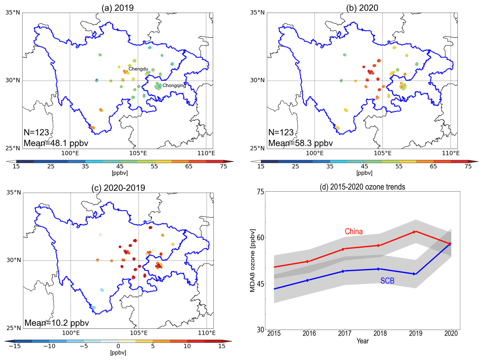
Figure 1Surface O3 enhancements over the SCB region in May–June 2020 relative to 2019. (a) Spatial distributions of May–June mean O3 concentrations over the SCB region in 2019. Number (N) denotes the available measurement sites for this year. We average the O3 concentrations at all measurement sites in each city to form an O3 dataset representative of the respective city. Panel (b) is the same as panel (a) but for 2020. Panel (c) shows the differences between 2020 and 2019. (d) Trends in May–June mean ozone concentrations from 2015 to 2020 averaged for all Chinese cities (red) and for the SCB city cluster (blue). Grey shading represents the mean ± 1σ SD across all cities. The base map of the figure was created using the Basemap package in Python.
After a continuous increase in surface-level O3 from 2013 to 2019, the summertime (May–August) O3 concentration across China showed a significant reduction in 2020 (Fig. 1d). In this study, we use high-resolution nested-grid GEOS-Chem simulation, the eXtreme Gradient Boosting (XGBoost) machine learning method, and the exposure–response relationship to determine the drivers and evaluate the health risks due to the unexpected surface O3 enhancements. We first use the XGBoost machine learning method to correct the GEOS-Chem model–measurement O3 discrepancy over the SCB. The relative contributions of meteorology and anthropogenic emission changes to the unexpected surface O3 enhancements are then quantified using a combination of the GEOS-Chem and XGBoost models. In order to assess the health risks caused by the unexpected O3 enhancements over the SCB, total premature mortalities are also estimated.
2.1 Surface O3 data and auxiliary data over the SCB
China has identified nine city clusters that show rapid population growth as well as advanced economical, societal, and cultural development with respect to the rest of the country. The SCB contains the fourth-largest city cluster in China after the Yangtze River Delta (YRD), the Pearl River Delta (PRD), and Beijing–Tianjin–Hebei (BTH). The location of the SCB city cluster is shown in Fig. S1 in the Supplement. With Chongqing and Chengdu as the dual core cities, more than a dozen cities over the SCB, including Mianyang, Deyang, Yibin, Nanchong, Dazhou, and Luzhou, have achieved rapid economic development and industrial upgrades. As the region with the strongest economic strength and best economic foundation in western China, the SCB region is home to many industries, such as the energy and chemical industry, electronic information, food processing, equipment manufacturing, ecotourism, and modern finance. Due to the fact that the SCB is one of the most densely populated and highly industrialized regions in China and owing to its basin terrain, which is favourable to the accumulation of air pollutants, the SCB is a newly emerging region of severe air pollution in China (K. D. Lu et al., 2019b, 2012).
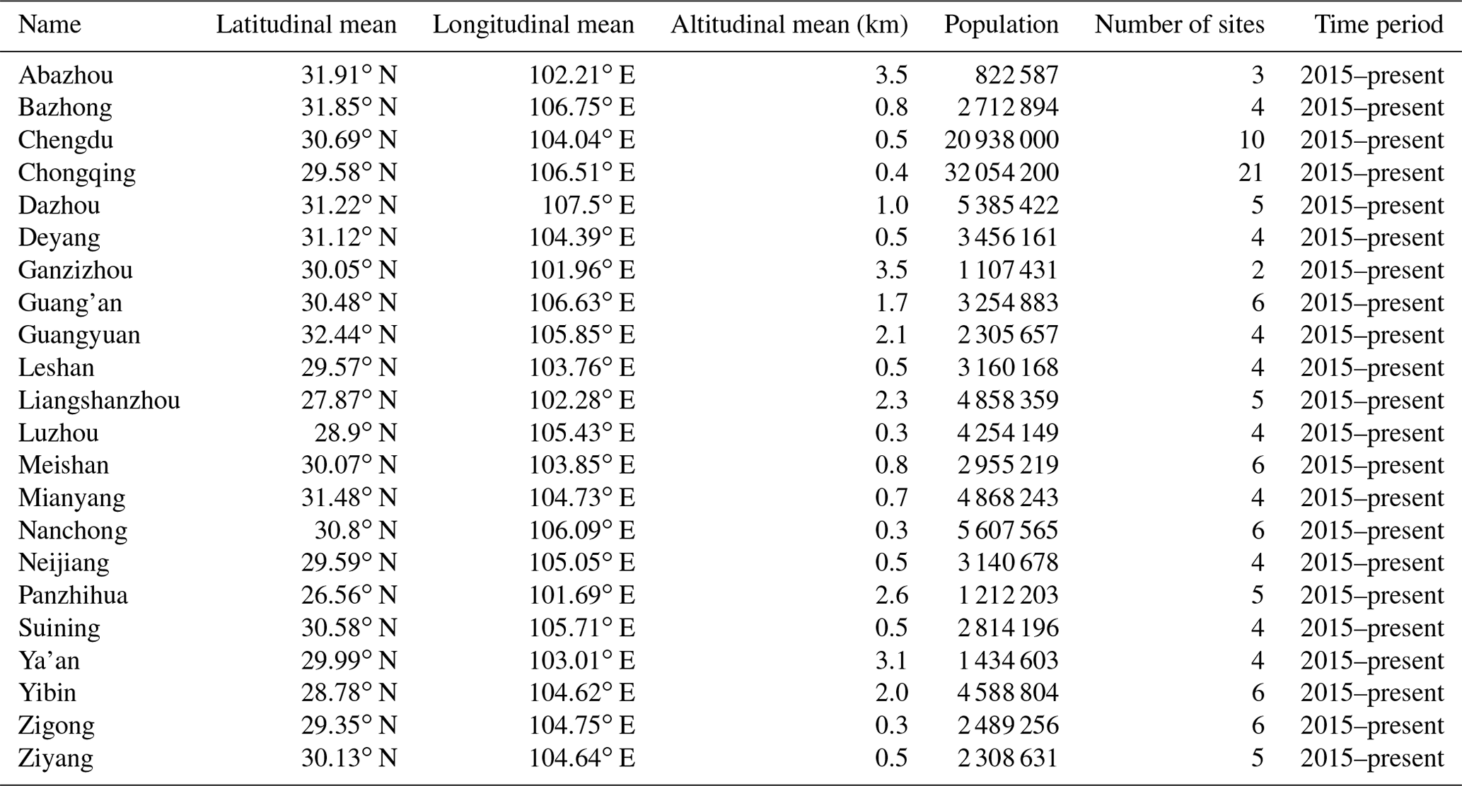
Surface O3 measurements over the SCB are available from the China National Environmental Monitoring Centre (CNEMC) network (http://www.cnemc.cn/en/, last access: 2 July 2021). The CNEMC network has routinely measured the concentrations of CO, O3, NO2, SO2, and particulate matter (PM10 and PM2.5) at 122 sites in 22 key cities over the SCB since 2015. The mean geolocation, population, the number of measurement sites, and the data range of each city are summarized in Table 1. The altitude of these cities ranges from 0.3 to 4.3 km a.s.l. (above sea level), and the population ranges from approximately 822 000 to 32.054 million. The number of measurement sites in each city ranges from 2 to 21. Surface O3 measurements at all measurement sites are based on similar differential absorption ultraviolet (UV) analysers. The hourly mean time series of surface O3 concentrations cover the period from January 2015 to present at all measurement sites in the 22 cities. After removing unreliable measurements with the filter criteria used in Lu et al. (2020) (see Sect. S1 in the Supplement for further details), we averaged the O3 concentrations at all measurement sites in each city to form an O3 dataset representative of the respective city. The O3 metric used in this study is the daily maximum 8 h average (MDA8).
Table 1Measurement sites in the SCB city cluster. All sites are organized alphabetically. Population statistics are based on the seventh nationwide population census in 2020 provided by National Bureau of Statistics of China.
As the vertical distributions of tropospheric HCHO and NO2 are weighted heavily toward the lower troposphere over polluted regions, many studies have used tropospheric column measurements of these gases to represent near-ground-level conditions (Streets et al., 2013; Sun et al., 2021b, 2018). In this study, the tropospheric NO2 and HCHO columns from the TROPOspheric Monitoring Instrument (TROPOMI) Level 3 products are used to investigate the changes in O3 precursors in May–June 2020 with respect to 2019. TROPOMI overpasses China at approximately 13:30 LT (local time) with a ground pixel size of 7×7 km. Pixels with quality assurance values of less than 50 % for HCHO and 75 % for NO2 are not included in present work.
2.2 GEOS-Chem nested-grid simulation
We use the high-resolution nested-grid GEOS-Chem model version 12.2.1 to simulate surface O3 over the SCB (Bey et al., 2001). Simulations are conducted at a horizontal resolution of 0.25∘ × 0.3125∘ over the nested domain (15–55∘ N, 70–140∘ E) covering China and the surrounding regions. The boundary conditions for the nested-grid GEOS-Chem simulation are archived from the global simulation at a 2∘ × 2.5∘ resolution (Sun et al., 2021a, b; Yin et al., 2019, 2020) We spun up the model for 1 year to remove the influence of the initial conditions. We first ran the global simulation at a 2∘ × 2.5∘ resolution and then interpolated the restart file on 1 January 2018 into high resolution (0.25∘ × 0.3125∘) for the nested domain in order to initialize the nested model simulation from January 2019 to June 2020.
The simulations were driven by the GEOS-FP meteorological field at the native resolution of 0.25∘ × 0.3125∘ with 47 layers from the surface to 0.01 hPa at the top. The PBLH and surface meteorological variables are implemented at 1 h intervals, and other meteorological variables are at 3 h intervals. The time step applied in the model for transport is 5 min, whereas the time step for chemistry and emissions is 10 min (Philip et al., 2016) The non-local scheme for the boundary layer mixing process is from Lin and McElroy (2010), wet deposition is from Liu et al. (2001), and dry deposition is generated with the resistance-in-series algorithm (Wesely, 1989; Zhang et al., 2001). The photolysis rates are from the FAST-JX v7.0 photolysis scheme (Bian and Prather, 2002). The chemical mechanism follows the universal tropospheric–stratospheric chemistry extension (UCX) mechanism (Eastham et al., 2014). The GEOS-Chem simulation outputs 47 layers of O3 and other atmospheric constituents over China with a temporal resolution of 1 h.
We use the Community Emissions Data System (CEDS) inventory for global anthropogenic emissions at the latest 2017 level, which is overwritten by the Chinese anthropogenic emissions with the Multi-resolution Emission Inventory for China (MEIC) in 2019 (Hoesly et al., 2018; Li et al., 2017; McDuffie et al., 2020; Zheng et al., 2018). Anthropogenic emissions are fixed for 2019 and 2020. Global BB and biogenic emissions were from the Global Fire Emissions Database (GFED v4) inventory (Giglio et al., 2013) and the Model of Emissions of Gases and Aerosols from Nature (MEGAN version 2.1) inventory (Guenther et al., 2012) respectively. Soil NOx emissions (Hudman et al., 2010; Lu et al., 2021) and lightning NOx (Murray et al., 2012) emissions are calculated online in the model.
2.3 Correction of the GEOS-Chem discrepancy using a machine learning method
We used the XGBoost machine learning method to correct the GEOS-Chem model–measurement O3 discrepancy over the SCB following Keller et al. (2021). The same methodology has also been applied in our companion study (Yin et al., 2021b) examining ozone changes over the eastern China from 2019 to 2020. It uses the Gradient Boosting Decision Tree (GBDT) framework to iteratively train the GEOS-Chem model–measurement discrepancy and improve the model predictions in a stage-wise manner. The XGBoost method minimizes the loss function by adding a weak learner to optimize the objective function. The optimization objective function used in XGBoost model is expressed as follows:
Here, gi and hi are the respective first- and second-order gradients of the loss function, L(t) represents the optimization objective function to be solved at the tth iteration, is the loss function representing the difference between the prediction for the ith sample at the (t-1)th iteration and the real values yi, and function f(t) is the amount of change at the tth iteration. Overall, the objective function consists of a two-order Taylor approximation expansion of the loss function and the regularization term (Ω(ft)), which penalizes the complexity of the model and prevents overfitting of the model. Compared with the traditional GBDT method, XGBoost method has the following advantages: it effectively handles missing values, it prevents overfitting, and it reduces computing time by using parallel and distributed computing methods.
As the GEOS-Chem model–measurement discrepancy is usually site-specific, we train a separate XGBoost model for each site. Similar to the method of Keller et al. (2021), we use a full seasonal cycle of hourly measurements in 2019 at each site as the learning samples, and we use GEOS-Chem input of emissions and meteorological parameters, output concentrations of atmospheric constituents, and time information as training input data. In order to properly incorporate emissions and meteorological factors that affect O3 production, we have included the GEOS-Chem simulated concentrations of 43 atmospheric chemical constituents, emissions of 21 atmospheric chemical constituents, 10 meteorological parameters, and 4 time parameters (e.g. hour, day, month, and year) into the data training. All of these training input data are summarized in Table S1 in the Supplement and have been standardized as shown in Eq. (2) in Sect. S2 in the Supplement. We choose a learning rate of 0.35, a maximum tree depth of 6, L1 and L2 regularization terms of 0 and 1, a mean square loss function, and the root-mean-square error (RMSE) evaluation metric in the data training.
We use the k-fold cross-validation method to test the performance of the XGBoost model (). First, all sample data are randomly and uniformly divided into k groups, where one group is taken as the test dataset and the remaining k-1 groups are taken as the training dataset. We then start to train the model and use the test dataset to evaluate the performance of the trained model. We repeated this process k times using different groups of datasets as the test data. The training model is finally determined if all of the k groups of experiments show similar performance. This method ensures the stability and robustness of the XGBoost model and avoids overfitting. In this study, a 10-fold cross-validation method is applied (i.e. we divide the O3 measurements in 2019 into 10 groups of sub-data): the training dataset accounts for 90 % of the total sample data, and the test dataset accounts for the remaining 10 %. We also attempted to use 60 % and 80 % of the sample data as the training dataset but did not find a significant influence on the results; this indicates the robustness of the XGBoost training model.
2.4 Quantifying meteorological and emission contributions
We have used the GEOS-Chem model only as well as a combination of the GEOS-Chem and XGBoost models (hereafter referred to as GEOS-Chem-XGBoost) to quantify the contributions of meteorology and anthropogenic emissions to the unexpected surface O3 enhancements over the SCB in 2020, following Yin et al. (2021b). For the GEOS-Chem method, as the anthropogenic emissions are fixed, the simulated O3 differences between 2020 and 2019 can be attributed to changes in meteorological conditions and are calculated as follows:
The contribution from anthropogenic emission changes can then be quantified as follows:
In the above-mentioned equations, G_Met and G_Emis represent the meteorology and anthropogenic emission contributions respectively, Meas2019 and Meas2020 represent O3 measurements in 2019 and 2020 respectively, and G2019 and G2020 represent GEOS-Chem O3 simulations in 2019 and 2020 respectively.
As the GEOS-Chem-XGBoost model has corrected the GEOS-Chem model–measurement discrepancy in 2019, we assume that it can provide accurate predictions of the surface O3 measurements in 2020 if the anthropogenic emissions remain unchanged. This assumption is valid because the probability density functions (PDFs) of key O3 precursors and meteorological parameters for the training data within a full seasonal cycle of 2019 cover the range of variation in these factors in May–June 2020 (Figs. S2 and S3 in the Supplement). To predict O3 evolution in 2020, all input parameters (except anthropogenic emissions) fed into each GEOS-Chem-XGBoost model are updated to match the measurements in 2020, whereas anthropogenic emissions are fixed at the 2019 levels. As a result, the differences between the GEOS-Chem-XGBoost predictions for 2020 and the 2020 measurements are attributed to the changes in anthropogenic emissions (Eq. 6). The meteorology-induced contributions are then obtained, as shown in Eq. (7), by subtracting the anthropogenic-emission-induced contributions.
In the above equations, the acronyms are similar to those in Eqs. (4) and (5) but for the GEOS-Chem-XGBoost method. By correcting the model–measurement discrepancy, the GEOS-Chem-XGBoost model is expected to provide a more accurate O3 sensitivity to changes in both meteorology and anthropogenic emissions as will be discussed later.
2.5 Health risks evaluation
We have assessed the total premature mortalities, including all non-accidental causes of death, hypertension, CVD, RD, COPD, and stroke, attributed to ambient O3 exposure in all cities in the SCB in 2019 and 2020. We first calculated the O3-induced daily premature mortalities based on the exposure–response relationship described in Cohen et al. (2004), which has been used in many subsequent studies (Anenberg et al., 2010; Liu et al., 2018; Wang et al., 2021). We then added up the daily premature mortalities within the May–June period and for the whole year respectively in order to get the total O3-induced premature mortalities in the respective periods. The population data used in this study include all age groups, which may result in higher daily mortalities than expected (Liu et al., 2018; Wang et al., 2021). According to Cohen et al. (2004), the daily premature mortalities attributable to ambient O3 exposure can be estimated using the following equation (Cohen et al., 2004):
where ΔM represents the daily premature mortalities due to ambient O3 exposure. The representative daily mean O3 concentration for a specific city Cmeas is an average of all of the measurements in the city. The variable y0 is the daily baseline mortality rate for each disease averaged from all ages and genders. We follow the method of Wang et al. (2021) and use the daily y0 value for each disease from the latest China Health Statistical Yearbook in 2018. β represents the increase in daily mortality as a result of each 10 µg cm3 (∼ 5.1 ppbv) increase in the daily O3 concentration, which has often been referred to as the concentration response function (CRF) in previous studies. We collected the CRF values from those used in Yin et al. (2017) and Wang et al. (2021). Δx represents the incremental O3 concentration relative to the threshold concentration Cthres of 35.1 ppbv, which is obtained from Lim et al. (2012) and Liu et al. (2018). “Pop” represents the population exposed to ambient O3 pollution and is available from the seventh nationwide population census in 2020, provided by National Bureau of Statistics of China. The daily y0 and β values for all non-accidental causes of death, hypertension, CVD, RD, COPD, and stroke are summarized in Table S2 in the Supplement.
Figures 1a and b show the May–June mean MDA8 O3 concentrations at all measurement sites in the SCB in 2019 and 2020. The May–June mean MDA8 O3 concentrations averaged over all cities in the SCB region in 2019 and 2020 are 48.1 and 58.3 ppbv respectively, which are 11.0 ppbv lower and 1.2 ppbv higher than those averaged over all Chinese cities during the corresponding periods. Due to the fact that the SCB is the most densely populated and highly industrialized region in western China, land use, industrialization, infrastructure construction, and urbanization in this region have expanded rapidly in recent years, resulting in the highest anthropogenic emissions of O3 precursors and the highest surface O3 levels being found in the area (Fig. S4 in the Supplement). Although the O3 levels in the SCB city cluster are lower than those in the three most developed city clusters in eastern China (i.e. the BTH; the Fenwei Plain, FWP; and the YRD), the SCB region has been classified by the Chinese Ministry of Environmental and Ecology (MEE) as a new pollution region with respect to O3 mitigation (Sun et al., 2021b; H. C. Wang et al., 2020; Wang and Lu, 2019; Zou et al., 2019). Due to the combination of basin topography, stationary meteorological fields, and high anthropogenic emissions, the SCB city cluster has the potential to develop frequent high-O3 events (such as those found in the BTH, FWP, and YRD).
We find significant O3 enhancements of 10.2 ± 0.8 ppbv (mean ± 1σ SD), or 23.4 %, averaged over all cities in the SCB in May–June 2020 with respect to the 2019 levels (Fig. 1c). The largest enhancements are observed in the most densely populated areas around the megacities of Chongqing and Chengdu (11.8 ± 0.6 ppbv, or 29.9 %). These year-to-year O3 enhancements over the SCB reach a record high in the 2015–2020 period, following an increasing change rate of 1.2 % yr−1 from 2015 to 2017 and then a decreasing change rate of −0.7 % yr−1 from 2017 to 2019. These surface O3 enhancements mainly reflect regional emissions and meteorology changes in the SCB and surrounding regions, as the lifetimes of surface O3 and most of its precursors are too short to undergo long-range transport.
The significant O3 enhancements over the SCB in May–June 2020 relative to 2019 are the inverse of the overall decrease in surface O3 levels across China during the same period (Fig. 1d). After a continuous increase in surface O3 levels from 2013 to 2019 by approximately 5 % yr−1 (Fig. 1d), the MDA8 O3 averaged over all cities outside of the SCB across China in May–June 2020 relative to 2019 levels showed a significant reduction of 5.3 ± 0.5 ppbv (8.3 %). Such O3 reductions are widespread in eastern China, especially in the BTH, FWP, and YRD regions, and we have investigated their drivers in a separate study (Yin et al., 2021b).
We use the normalized root-mean-square error (NRMSE), normalized mean bias (NMB), and Pearson correlation coefficient (R) to assess the performance of the GEOS-Chem-XGBoost model. For each measurement site, we analysed these metrics for both training (blue) and test (red) datasets, as shown in Fig. S5 in the Supplement. We define the NRMSE as the RMSE normalized by the difference between the 95th and 5th percentile concentrations, and we define the NMB as the mean bias normalized by average concentration at the given measurement site. The formulas for the above-mentioned metrics are summarized in Sect. S2 in the Supplement.
The GEOS-Chem-XGBoost model predictions for surface O3 over the SCB show no bias when evaluated against the training data, with an NMB of 0.01, NRMSE values of less than 0.1, and an R value between 0.93 and 1.0. Compared with the training data, the performance on the test data shows a higher variability, with an average NMB of −0.04, an NRMSE of 0.22, and an R of 0.83. We find no significant difference in predictive performance between clean (less than the Cthres defined in Sect. 2.5) and polluted measurement sites. A number of factors likely contribute to the relatively poorer statistical results at some sites such as Ganzizhou, Leshan, and Suining. First, the training data for these sites may include certain temporal events that are not easily generalizable, such as unusual emission activity (e.g. BB, fireworks, and the closure of nearby point sources) or weather patterns that are not properly observed, which might be prone to overfitting. In addition, the differences in surface O3 variabilities between the training data and the test data at these sites are relative larger than at other sites, which can contribute to a relative poorer performance.

Figure 2The importance of input variables for the XGBoost model trained to correct the GEOS-Chem model–measurement O3 discrepancy over the SCB. Shown are the distribution of the SHAP values for each variable averaged over all cities in the SCB, ranked by the average importance of each feature. A higher SHAP value indicates higher feature importance. The acronyms are defined in Table S1. For clarity, only the top 30 variables are shown. See Fig. S6 in the Supplement for the relative importance of all variables.
We use the SHapely Additive exPlanations (SHAP) approach to examine how the GEOS-Chem-XGBoost model uses the input variables to make a prediction. The SHAP approach is based on game-theoretic Shapely values and represents a measure of each predictor's responsibility for a change in the model prediction (Lundberg and Lee, 2017). The SHAP values are computed separately for each model prediction and offer detailed insight into the importance of each input variable for this prediction while also considering the role of variables interactions (Keller et al., 2021; Lundberg et al., 2020). Figure 2 shows the SHAP value distribution for all of the major O3 predictors averaged over all cities in the SCB. The results show that all variables that are expected to be associated with O3 formation can affect model O3 prediction. Generally, the temperatures (at the surface, 2 m height, and 10 m height) are the most important predictors for the GEOS-Chem model–measurement discrepancy over the SCB, followed by the uncorrected GEOS-Chem-simulated O3, reactive nitrogen (e.g. NO2 and peroxyacetyl nitrate – PAN), atmospheric oxidants (Ox and hydrogen peroxide – H2O2), fine aerosols, VOCs (isoprene and propane – C3H8), hour of the day, and meteorological variables including horizontal and vertical wind speeds (u10 m, v10 m). All of these factors have tight connections to surface O3 formation over the SCB; thus, it is not surprising that the GEOS-Chem model–measurement discrepancies are most sensitive to them (Seinfeld and Pandis, 2016).
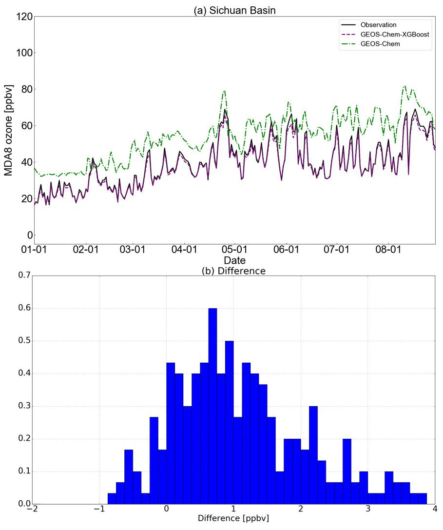
Figure 3Measured and modelled O3 variability over the SCB in 2019 (a). Measured, GEOS-Chem-predicted, and GEOS-Chem-XGBoost-predicted O3 values are denoted by black solid, grey dashed, and purple dashed lines respectively. Panel (b) presents a histogram of the differences between the GEOS-Chem-XGBoost predictions and the measurements.
We have compared the performance of GEOS-Chem and GEOS-Chem-XGBoost with respect to capturing the measured surface O3 levels. Figure 3a shows the time series of measured and model-predicted O3 concentrations averaged over all cities in the SCB region. Figure 3b shows a histogram of the differences between the GEOS-Chem-XGBoost predictions and the measurements. The GEOS-Chem simulations generally capture the daily variability in MDA8 O3 over the SCB, but they show a high bias of 7.8 ± 5.0 ppbv (17.5 %) across all measurement sites within the SCB region. The discrepancy can be mainly attributed to uncertainties in the horizontal transport and vertical mixing schemes simulated by the GEOS-Chem model at a relatively coarse spatial resolution compared with the measurements at a single point, but it can also be associated with the errors in emission estimates, the chemical mechanism, and the sub-grid-scale local meteorological processes. Specifically, errors in O3 predictors with high SHAP values are more likely to result in a large model–measurement discrepancy. For example, the GEOS-Chem model overestimates the correlations between the surface O3 concentration and temperature (Fig. S7a in the Supplement), indicating that this overestimation of the O3 temperature sensitivity is one of the major factors contributing to higher GEOS-Chem model O3 predictions.
By iteratively training and correcting the GEOS-Chem model–measurement discrepancy in the O3 temperature sensitivity, the correlations between temperature and the surface O3 concentration predicted by the GEOS-Chem-XGBoost model were in good agreement with the measurements (Fig. S7a). With respect to the performance of reproducing the sensitivities of O3 to other meteorological parameters such as humidity, cloud fraction, and precipitation, the GEOS-Chem-XGBoost model is also better than the GEOS-Chem model (Fig. S7b–d). After correcting the errors in all O3 predictors, the GEOS-Chem-XGBoost model significantly improves the prediction of surface O3 concentrations in all cities over the SCB compared with GEOS-Chem (Fig. S8 in the Supplement). It shows a bias of 0.5 ± 0.3 ppbv for all O3 measurements in 2019 over the SCB. As a result, the overall GEOS-Chem-XGBoost model performance is acceptable and can support further investigation of the drivers of the unexpected surface O3 enhancements over the SCB in May–June 2020.
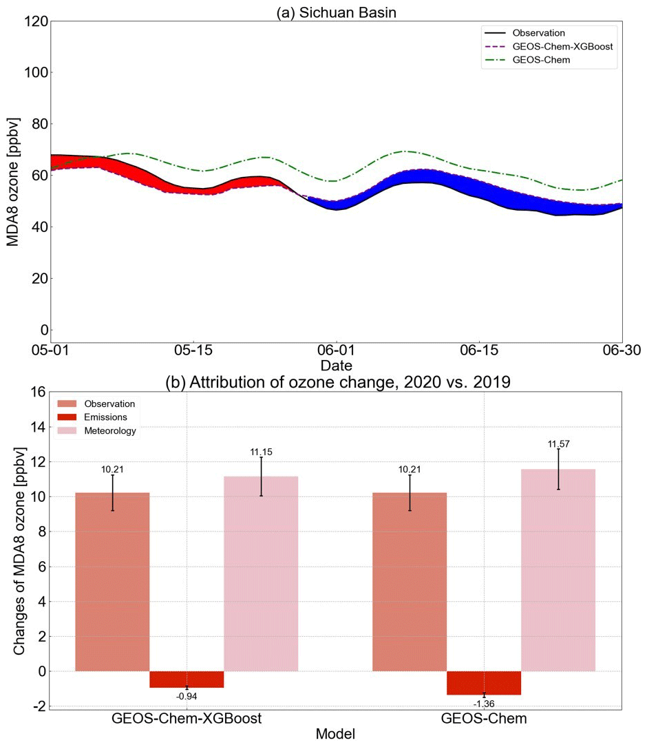
Figure 4(a) Comparison of the GEOS-Chem-XGBoost O3 predictions with the 2020 measurements. Red (blue) shading represents periods when GEOS-Chem-XGBoost predictions are higher (lower) than the actual measurements in 2020, indicating that changes in anthropogenic emissions led to an O3 increase (decrease) in 2020. All values shown are 7 d averages for presentation purposes. (b) Attribution of surface O3 enhancements over the SCB in May–June 2020 relative to 2019. Filled coloured bars denote O3 change as seen from measurements as well as O3 change due to changes in anthropogenic emissions and meteorological conditions estimated by the GEOS-Chem-XGBoost model and the GEOS-Chem model. Black vertical bars represent 1σ SD across cities.
5.1 Separation of meteorological and anthropogenic emission contributions
We quantify the surface O3 enhancements in May–June 2020 over the SCB to changes in anthropogenic emissions and meteorological conditions according to Eqs. (6) and (7) respectively. Differences between the measured and GEOS-Chem-XGBoost-predicted O3 in May–June 2020, as indicated by the shaded areas in Fig. 4a, represent the anthropogenic-emission-induced O3 changes in 2020 relative to 2019. The mean contributions driven by changes in anthropogenic emissions and meteorological conditions are summarized in Fig. 4b. Due to the different change rates in anthropogenic emissions in May and June 2020 (see Sect. 5.3), the changes in anthropogenic emissions caused an overall increase in the surface O3 level in May but a reduction in the surface O3 level in June (Fig. 4a). For the May–June mean contributions averaged over all cities in the SCB, changes in anthropogenic emissions caused a 0.9 ± 0.1 ppbv O3 reduction, and changes in meteorology caused a 11.1 ± 0.7 ppbv O3 increase; these values correspond to −8.0 % and 108 % of the relative contributions to the total O3 enhancement (10.2 ± 0.8 ppbv) over the SCB in May–June 2020 respectively. As a result, the anthropogenic-emission-induced O3 reductions are dominantly overwhelmed by the meteorology-induced O3 increases, leading to the unexpected O3 enhancements over the SCB in 2020.
We compare the meteorology-induced and anthropogenic-emission-induced contributions to the unexpected surface O3 enhancements estimated by the GEOS-Chem-XGBoost model and to those estimated by the GEOS-Chem model only (Fig. 4b). Both methods show that changes in meteorology contribute significantly to the O3 enhancements, although the absolute magnitudes differ slightly from each other. For example, the anthropogenic-emission-induced O3 reduction calculated with the GEOS-Chem model only is 0.94 ppbv, whereas the value calculated with the GEOS-Chem-XGBoost model is 1.36 ppbv. Using the subtraction in Eq. (5) and the average over all cities, the propagation of systematic model discrepancies that are common to all measurements sites was effectively minimized, which can mitigate the difference in attribution results between the GEOS-Chem and GEOS-Chem-XGBoost methods. However, as demonstrated in Fig. S8, model discrepancies may differ between regions and time periods. Therefore, the GEOS-Chem-XGBoost approach is expected to provide a more accurate and consistent estimate of O3 change attribution than the GEOS-Chem model alone.

Figure 5Terrain elevations (a) and surface temperature and wind fields (b) over the SCB and surrounding regions. The spatial resolutions for panels (a) and (b) are 3 × 3 arcmin and 0.25∘ × 0.25∘ respectively. In panel (a), the white area is the Tibetan Plateau (with altitudes of 4–5 km a.s.l.), the yellow area is the Yunnan–Kweichow Plateau (2–3 km a.s.l), and the green area is the SCB (0.5–1 km a.s.l). The base map of the figure was created using the Basemap package in Python.
5.2 Meteorological contribution
Figure 5 shows the terrain elevations and May–June mean wind fields and surface pressures over the SCB and surrounding regions. The terrain altitudes, at a resolution of 3 × 3 arcmin, indicate a rapid change in altitude from the Tibetan Plateau (4.0–5.0 km) and Yunnan–Kweichow Plateau (2–3 km) to the SCB (0.5 km). The SCB is located in the saddle between the Tibetan Plateau and the Yunnan–Kweichow Plateau (Chen et al., 2009; Sun et al., 2021c). Figure 5b shows the May–June mean wind fields at 500 m overlaid with surface pressure available from GEOS-FP fields at a 0.25∘ × 0.3125∘ resolution. In May–June, the Tibetan high forms over the middle region of the Tibetan Plateau and the western Pacific subtropical high shifts westward to the west of the SCB (Chen et al., 2009). The southwesterly East Asian summer monsoon generates a cyclonic pattern over the southeastern part of the SCB. Driven by large-scale circulations, southwesterly flow enters the eastern part of the SCB near the northwestern edge of the Yunnan–Kweichow Plateau, while strong northwesterly flow enters the SCB near the eastern edge of the Tibetan Plateau. The interaction of these two flows results in a convergent zone of northward jet stream over the eastern part of the SCB due to the westward shift in the western Pacific subtropical high and the blocking effect of topography. Furthermore, strong instability of vertical convection could originate over the basin and move toward the eastern part of the SCB as dry air continuously enters the upper layer over the SCB (Chen et al., 2009). This process makes the SCB a favourable region for trapping air pollutants (Chen et al., 2009; Liu et al., 2003).
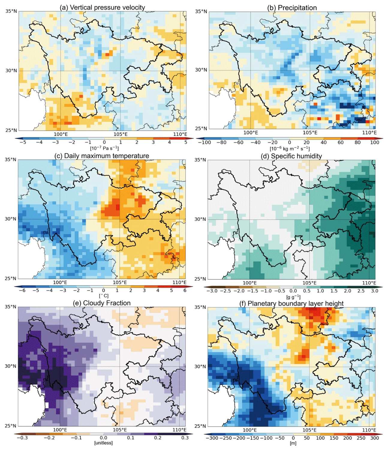
Figure 6May–June mean differences in vertical pressure velocity (a), precipitation (b), temperature (c), specific humidity (d), cloud fraction (e), and PBLH (f) between 2020 and 2019 over the SCB and surrounding regions. All of these meteorological parameters are from the GEOS-FP dataset. The vertical pressure velocity is prescribed at the PBLH, whereas the other parameters are prescribed at the surface. The base map of the figure was created using the Basemap package in Python.
Figure 6 shows the May–June mean differences in vertical velocity, precipitation, temperature, specific humidity, cloud fraction, and the PBLH between 2020 and 2019. In May–June 2020, the northwestern, central western, and southern areas of China experienced anomalous strong droughts (https://quotsoft.net/air/, last access: 12 June 2021.), leading to a significant increase in temperature and decreases in precipitation, specific humidity, and cloud fractions compared with the 2019 levels (Fig. 6). These changes in meteorological conditions could enhance the natural emissions of O3 precursors and speed up O3 chemical production. Meanwhile, the SCB basin effect inhibited the ventilation of O3 and its precursors, which further enhanced O3 accumulation over the SCB. As a result, we conclude that the meteorological anomalies combined with the complex basin effect caused the surface O3 enhancements over the SCB in 2020. Although a higher PBLH over the SCB in May–June 2020 relative to 2019 may have reduced surface O3 levels by diluting O3 and its precursors into a larger volume of air, this reduction effect was overwhelmed by the aforementioned enhancement effect. There is no strong evidence of a change in the horizontal transport from other regions (Fig. 5b) or the vertical transport from the free troposphere to the surface (Fig. 6a) over the SCB in May–June 2020 relative to 2019 (Lefohn et al., 2012; Skerlak et al., 2014; Stohl et al., 2003; H. C. Wang et al., 2020; H. Y. Wang et al., 2020; P. Wang et al., 2020; Wang and Lu, 2019; Wirth and Egger, 1999). It is worth noting that, with similar meteorological anomalies in May–June 2020 relative to 2019, O3 enhancements were not observed in northwestern China, such as the Xinjiang Uygur Autonomous Region and the Inner Mongolia Autonomous Region, or in southern China, such as the Pearl River Delta (PRD) region, which is also one of the nine well-developed city clusters in China with severe air pollution. This can be partly attributed to low anthropogenic emissions of O3 precursors in northwestern China (Zheng et al., 2018) and to the fact that strong land–sea exchange, driven by the summer monsoon, in coastal regions facilitates the ventilation of O3 and its precursors in the PRD region. Furthermore, the meteorology-induced O3 enhancements are probably overwhelmed by the anthropogenic-emission-induced O3 reductions in northwestern and southern China.
5.3 Emission contribution
To suppress the spread of coronavirus (COVID-19) in China during the pandemic in 2019, the Chinese government sealed off several cities starting in January 2020; this included implementing a measures such as closing local businesses and halting public transportation at an unprecedented scale (Li et al., 2019b; Steinbrecht et al., 2021; Yin et al., 2021a). These prevention measures quickly spread nationwide. Although the COVID-19 lockdowns in all cities were lifted before May, there were still restrictions on public transportation, businesses, social activities, and industrial manufacturing, which could have caused domestic anthropogenic emission reductions in both HCHO and NOx. Furthermore, the MEE continues to mitigate NOx emissions following the 2018–2020 action plan to defend blue skies, and it has also implemented the 2020 action plan to mitigate VOCs. This new action plan issues a number of control measures including the implementation of stringent VOC emission standards, the replacement of raw and auxiliary materials with a low VOC content, and the mitigation of unorganized emissions (emissions that are discharged without passing through an exhaust cylinder or stack). Driven by the above-mentioned factors, the TROPOMI-observed tropospheric HCHO and NO2 over China in May–June 2020 decreased by 2.0 ± 0.3 % (averaged for all Chinese cities) and 1.1 ± 0.2 % relative to 2019 respectively. Due to the relative short lifetime of both HCHO and NO2 in the troposphere, these reductions mostly reflect local emission changes. These reductions in domestic anthropogenic emissions dominated the significant reduction in summertime MDA8 O3 across China in 2020 relative to 2019.
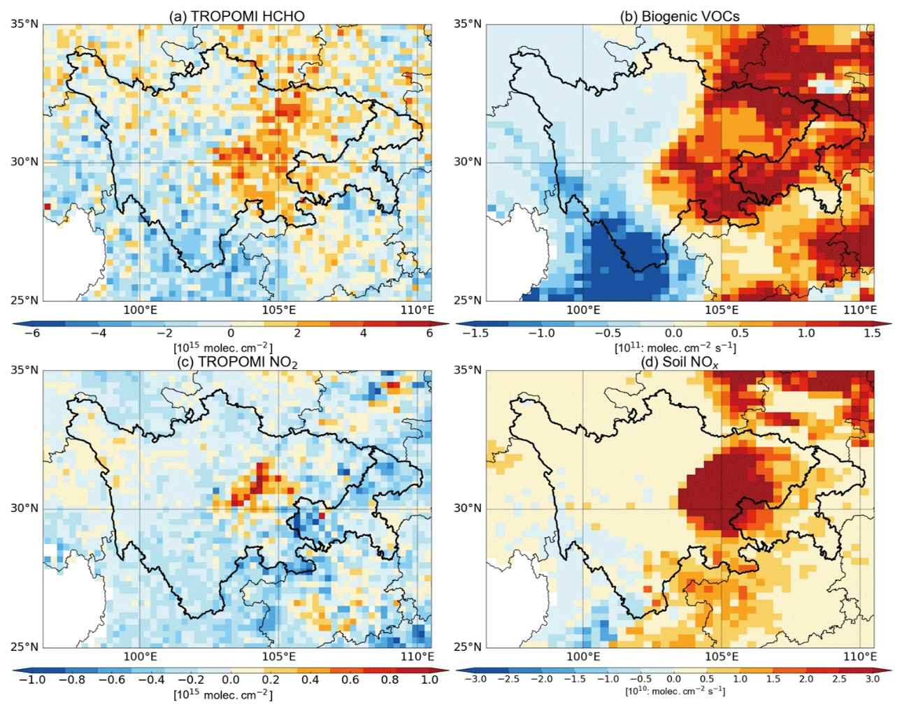
Figure 7May–June mean differences in O3 precursors between 2020 and 2019: (a) TROPOMI-observed HCHO, (b) biogenic VOCs, (c) TROPOMI-observed NO2, and (d) soil NOx. Biogenic VOCs and soil NOx are available from GEOS-Chem model online calculations. The base map of the figure was created using the Basemap package in Python.
Following the method of Sun et al. (2018), we have used the ratios to investigate the O3 production regime over the SCB region. The results show that the satellite observations of ratios in May–June in most cities over the SCB indicate a shift toward high values from 2019 to 2020, but the O3 chemical sensitivity in 2020 still lies within the transitional regime (Fig. S9, in the Supplement; Jin et al., 2017; Jin and Holloway, 2015). Meanwhile, the O3 chemical sensitivity in May 2020 is similar to that in June, indicating that the O3 variability in May–June 2020 is sensitive to both NOx and VOCs. The recently available Chinese statistical data on anthropogenic emissions provided by the MEE show that the anthropogenic VOC concentrations over the SCB have decreased by 5.0 % and 3.5 % in May and June in 2020 relative to the 2019 level respectively. The anthropogenic NOx increased by 1.5 % and decreased by 1.7 % during the same periods respectively (Zheng et al., 2021). The increase in anthropogenic NOx in May 2020 relative to 2019 is attributed to an increase in NOx emissions from the power plant sector, which was not affected by the post-lockdown restrictions to suppress the spread of COVID-19 (Table S3 in the Supplement). For the May–June aggregation, the anthropogenic VOC and NOx emissions over the SCB decreased by 4.3 % and 0.3 % respectively (Zheng et al., 2021). These independent analyses of the anthropogenic emissions explain the different predicted O3 changes due to anthropogenic emissions alone in May (increase) vs. June (decrease) in the SCB.
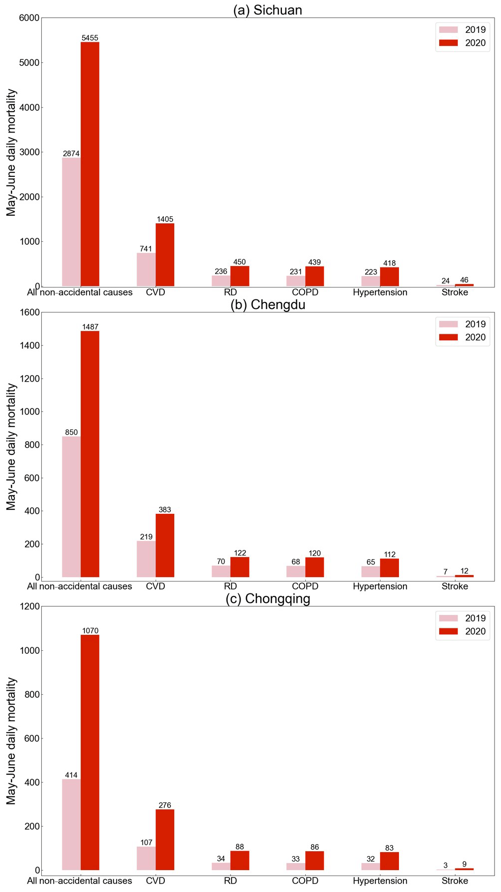
Figure 8Total daily mortality from all non-accidental causes of death, CVD, RD, COPD, hypertension, and stroke attributable to ambient O3 exposure over the SCB during May–June in 2019 and 2020.
In contrast to the widespread reductions in both HCHO and NO2 across the BTH, FWP, and YRD regions, we find notable increases in both HCHO and NO2 in the SCB in May–June 2020 relative to the 2019 levels. The tropospheric HCHO and NO2 columns averaged over all cities in the SCB region increased by (2.8 ± 0.3 %) and (5.1 ± 0.5 %) in 2020 relative to the 2019 levels respectively. As both anthropogenic VOC and NOx emissions in the SCB showed decreasing change rates in May–June 2020 relative to 2019, these regional increases in both HCHO and NO2 could be attributed to natural emission enhancements in both VOCs and NO2. Indeed, natural emissions of biogenic VOCs and soil NOx calculated online in the GEOS-Chem model show increasing change rates in May–June 2020 relative to 2019 in the SCB and surrounding regions (Fig. 7). These enhanced biogenic VOC and NOx emissions are most likely driven by the hotter and dryer meteorological conditions in area (Fig. 7).
Finally, we concluded that natural emission enhancements of both NOx and VOCs induced by the unexpected meteorological anomalies could account for the O3 enhancements in May–June 2020 over the SCB, and their contributions have been included in the meteorology-driven ozone enhancement as discussed in Sect. 5.2. However, in present work, we were not able to determine which specific VOC species are the most relevant for O3 enhancements nor could we quantify the relative contributions of VOC and NOx enhancements to O3 enhancements in the SCB. A series of sensitivity studies might be able to address this important issue, but this is beyond the scope of present work.
Figure 8 presents the total premature mortalities from all non-accidental causes of death, hypertension, CVD, RD, COPD, and stroke attributable to ambient O3 exposure in all cities over the SCB during May–June in 2019 and 2020. The statistical results for each city in 2019 and 2020 are summarized in Tables S4 and S5 in the Supplement respectively. The surface O3 enhancements over the SCB in May–June 2020 relative to 2019 result in dramatically higher health risks. The estimated total premature mortalities from all non-accidental causes of death due to surface O3 enhancements in May–June 2020 over the SCB is 5455, which is 89.8 % higher than that in the same period in 2019 (i.e. 2874). All of the above-mentioned O3-induced diseases over the SCB have significant increases in total mortalities in May–June 2020 relative to 2019. The highest health risk among these diseases is from CVD, which is 741 in May–June 2019, followed by RD (236), COPD (231), and hypertension (223). This O3-induced health risk rank over the SCB is consistent with those in the YRD, BTH, and PRD reported in previous studies (Liu et al., 2018; Lu et al., 2020; Yin et al., 2017; Wang et al., 2021). In May–June 2020, total mortalities from CVD, RD, COPD, hypertension, and stroke over the SCB reached respective values of 1405, 450, 439, 418, and 46 due to significant O3 enhancements. The change rates for these diseases are 89.6 %, 90.7 %, 90.1 %, 87.4 %, and 91.7 % respectively.
From a whole-year view, the estimated total premature mortalities from all non-accidental causes of death due to surface O3 exposure over the SCB in 2019 and 2020 are 16 772 and 18 301 respectively (Tables S4 and S5). All O3-induced diseases within May–June 2019 account for about ∼ 17.0 % of those for the whole year in 2019, and this percentage reaches up to ∼ 30.0% in 2020 (Fig. S10 in the Supplement). The total premature mortalities from all non-accidental causes of death due to surface O3 exposure over the SCB increased by 1528 for the whole year in 2020 relative to 2019 (Fig. S11 in the Supplement), which is 40.8 % lower than that within the May–June period in 2020 relative to 2019 (i.e. 2581). This indicates that the O3 level over the SCB showed an overall decreasing change rate in all months except May–June in 2020 relative to 2019, which resulted in a decrease (by 1053) in O3-induced diseases during the period.
We further investigated the O3-induced diseases in the two most densely populated cities in the SCB (i.e. Chengdu and Chongqing) during May–June in 2019 and 2020. The premature mortalities from all O3-induced diseases in each city in 2020 (relative to 2019) are dependent on the regional population, the surface O3 level, and the enhancement level (Eq. 9). Due to the fact that they have the largest populations and highest O3 enhancements, the estimated total premature mortalities in Chengdu and Chongqing accounted for 46.9 % of total O3-induced mortalities in the SCB during May–June 2020 (Fig. 8b, c). As the O3 levels and enhancement in Chengdu are larger than those in Chongqing, the total O3-induced mortalities in Chengdu are higher, even with the area's smaller population. The change rates for all O3-induced diseases are about 75 % in Chengdu and 160 % in Chongqing during May–June 2020 relative to 2019, which are much higher than the enhancement of ozone levels in the two cities (29.9 %). In order to reduce the O3-induced health risk, strident O3 control policies are necessary in densely populated cities.
Understanding the drivers and health risks of surface high-O3 events has strong implications for O3 mitigation. After a continuous increase in the surface O3 level from 2013 to 2019, the overall summertime O3 concentration across China showed a significant reduction in 2020. In contrast to this overall reduction in surface-level O3 across China, unexpected surface O3 enhancements of 10.2 ± 0.8 ppbv (23 %) were observed in May–June 2020 (relative to 2019) over the Sichuan Basin (SCB), China. In this study, we have used high-resolution nested-grid GEOS-Chem simulation, the eXtreme Gradient Boosting (XGBoost) machine learning method, and the exposure–response relationship to determine the drivers and evaluate the health risks of the unexpected surface O3 enhancements.
By iteratively training and correcting the GEOS-Chem model–measurement discrepancies, the GEOS-Chem-XGBoost model significantly improves the prediction of surface O3 concentrations compared with the GEOS-Chem. It shows a bias of 0.5 ± 0.3 ppbv against all O3 measurements over the SCB. As a result, the overall GEOS-Chem-XGBoost model performance is acceptable and can support further investigation of the drivers of unexpected surface O3 enhancements over the SCB in May–June 2020. The results show that changes in anthropogenic emissions caused a 0.9 ± 0.1 ppbv O3 reduction and that changes in meteorology caused a 11.1 ± 0.7 ppbv O3 increase. The meteorology-induced surface O3 increase is mainly attributed to an increase in temperature and decreases in precipitation, specific humidity, and cloud fractions over the SCB and surrounding regions in 2020 relative to the 2019 levels. These changes in meteorology combined with the complex SCB basin effect enhanced biogenic emissions of VOCs and NOx, sped up O3 chemical production, and inhibited the ventilation of O3 and its precursors, thereby causing surface O3 enhancements over the SCB.
The unexpected surface O3 enhancements over the SCB in May–June 2020 relative to 2019 resulted in dramatically higher health risks. The estimated total premature mortalities due to these events in the SCB during May–June 2020 is 5455, which is 89.8 % higher than that in the same period in 2019 (i.e. 2874). We further investigated the O3-induced diseases in the two most densely populated cities over the SCB (i.e. Chengdu and Chongqing) during May–June in 2019 and 2020. Due to the fact that these cities have the largest populations and highest O3 enhancements, the estimated total premature mortalities in Chengdu and Chongqing accounted for 46.9 % of total O3-induced mortalities over the SCB. The change rates for all O3-induced diseases are about 75 % in Chengdu and 160 % in Chongqing during May–June 2020 relative to 2019, which are much higher than the enhancement of ozone levels in the two cities (29.9 %). In order to reduce the O3-induced health risks, strident O3 control policies are necessary in densely populated cities.
The data are available upon request from Youwen Sun (ywsun@aiofm.ac.cn).
The supplement related to this article is available online at: https://doi.org/10.5194/acp-21-18589-2021-supplement.
YS designed the study and wrote the paper. HY carried out the GEOS-Chem simulations and the GEOS-Chem-XGBoost training and evaluation. BZ constructed the latest MEIC emission inventory. XL, JN, MP, CL, and YT provided constructive comments.
The contact author has declared that neither they nor their co-authors have any competing interests.
Publisher’s note: Copernicus Publications remains neutral with regard to jurisdictional claims in published maps and institutional affiliations.
This article is part of the special issue “Air quality research at street level (ACP/GMD inter-journal SI)”. It is not associated with a conference.
The authors would also like to thank Wernli Heini and the two anonymous referees for their valuable comments that improved the quality of this paper.
This work has been jointly supported by the National Key Research and Development Program of China (grant no. 2019YFC0214802), the Youth Innovation Promotion Association of the Chinese Academy of Sciences (grant no. 2019434), and the Sino-German Mobility programme (grant no. M-0036).
This paper was edited by Karine Sartelet and reviewed by two anonymous referees.
Akimoto, H., Mori, Y., Sasaki, K., Nakanishi, H., Ohizumi, T., and Itano, Y.: Analysis of monitoring data of ground-level ozone in Japan for long-term trend during 1990–2010: Causes of temporal and spatial variation, Atmos. Environ., 102, 302–310, https://doi.org/10.1016/j.atmosenv.2014.12.001, 2015.
Anenberg, S. C., Horowitz, L. W., Tong, D. Q., and West, J. J.: An Estimate of the Global Burden of Anthropogenic Ozone and Fine Particulate Matter on Premature Human Mortality Using Atmospheric Modeling, Environ. Health Persp., 118, 1189–1195, 2010.
Atkinson, R.: Atmospheric chemistry of VOCs and NOx, Atmos. Environ., 34, 2063–2101, 2000.
Bey, I., Jacob, D. J., Yantosca, R. M., Logan, J. A., Field, B. D., Fiore, A. M., Li, Q. B., Liu, H. G. Y., Mickley, L. J., and Schultz, M. G.: Global modeling of tropospheric chemistry with assimilated meteorology: Model description and evaluation, J. Geophys. Res.-Atmos., 106, 23073–23095, https://doi.org/10.1029/2001jd000807, 2001.
Bian, H. S. and Prather, M. J.: Fast-J2: Accurate simulation of stratospheric photolysis in global chemical models, J. Atmos. Chem., 41, 281–296, 2002.
Brauer, M., Freedman, G., Frostad, J., van Donkelaar, A., Martin, R. V., Dentener, F., van Dingenen, R., Estep, K., Amini, H., Apte, J. S., Balakrishnan, K., Barregard, L., Broday, D., Feigin, V., Ghosh, S., Hopke, P. K., Knibbs, L. D., Kokubo, Y., Liu, Y., Ma, S. F., Morawska, L., Sangrador, J. L. T., Shaddick, G., Anderson, H. R., Vos, T., Forouzanfar, M. H., Burnett, R. T., and Cohen, A.: Ambient Air Pollution Exposure Estimation for the Global Burden of Disease 2013, Environ. Sci. Technol., 50, 79–88, 2016.
Chen, D., Wang, Y., McElroy, M. B., He, K., Yantosca, R. M., and Le Sager, P.: Regional CO pollution and export in China simulated by the high-resolution nested-grid GEOS-Chem model, Atmos. Chem. Phys., 9, 3825–3839, https://doi.org/10.5194/acp-9-3825-2009, 2009.
Chen, X. R., Wang, H. C., Lu, K. D., Li, C. M., Zhai, T. Y., Tan, Z. F., Ma, X. F., Yang, X. P., Liu, Y. H., Chen, S. Y., Dong, H. B., Li, X., Wu, Z. J., Hu, M., Zeng, L. M., and Zhang, Y. H.: Field Determination of Nitrate Formation Pathway in Winter Beijing, Environ. Sci. Technol., 54, 9243–9253, 2020.
Cohen, A. J., Anderson, H. R., Ostro, B., Pandey, K. D., Krzyzanowski, M., Künzli, N., Gutschmidt, K., Pope, A., Romieu, I., Samet, J. M., and Smith, K.: Urban air pollution, in: Comparative quantification of health risks, Global and regional burden of disease attributable to selected major risk factors, edited by: M. Ezzati, A. D. Lopez, A. Rodgers, and C. J. L. Murray, World Health Organization, Geneva, 1, 1353–1433, ISBN 978-9-2415-8031-1, 2004.
Cooper, O. R.: Detecting the fingerprints of observed climate change on surface ozone variability, Sci. Bull., 64, 359–360, 2019.
Eastham, S. D., Weisenstein, D. K., and Barrett, S. R. H.: Development and evaluation of the unified tropospheric-stratospheric chemistry extension (UCX) for the global chemistry-transport model GEOS-Chem, Atmos. Environ., 89, 52–63, 2014.
Fleming, Z. L., Doherty, R. M., von Schneidemesser, E., Malley, C. S., Cooper, O. R., Pinto, J. P., Colette, A., Xu, X. B., Simpson, D., Schultz, M. G., Lefohn, A. S., Hamad, S., Moolla, R., Solberg, S., and Feng, Z. Z.: Tropospheric Ozone Assessment Report: Present-day ozone distribution and trends relevant to human health, Elementa-Sci. Anthrop., 6, 2, https://doi.org/10.1525/elementa.273, 2018.
Fu, T.-M., Zheng, Y., Paulot, F., Mao, J., and Yantosca, R. M.: Positive but variable sensitivity of August surface ozone to large-scale warming in the southeast United States, Nat. Clim. Change, 5, 454–458, https://doi.org/10.1038/nclimate2567, 2015.
Giglio, L., Randerson, J. T., and van der Werf, G. R.: Analysis of daily, monthly, and annual burned area using the fourth-generation global fire emissions database (GFED4), J. Geophys. Res.-Biogeo., 118, 317–328, https://doi.org/10.1002/jgrg.20042, 2013.
Guenther, A., Karl, T., Harley, P., Wiedinmyer, C., Palmer, P. I., and Geron, C.: Estimates of global terrestrial isoprene emissions using MEGAN (Model of Emissions of Gases and Aerosols from Nature), Atmos. Chem. Phys., 6, 3181–3210, https://doi.org/10.5194/acp-6-3181-2006, 2006.
Guenther, A. B., Jiang, X., Heald, C. L., Sakulyanontvittaya, T., Duhl, T., Emmons, L. K., and Wang, X.: The Model of Emissions of Gases and Aerosols from Nature version 2.1 (MEGAN2.1): an extended and updated framework for modeling biogenic emissions, Geosci. Model Dev., 5, 1471–1492, https://doi.org/10.5194/gmd-5-1471-2012, 2012.
He, J. J., Gong, S. L., Yu, Y., Yu, L. J., Wu, L., Mao, H. J., Song, C. B., Zhao, S. P., Liu, H. L., Li, X. Y., and Li, R. P.: Air pollution characteristics and their relation to meteorological conditions during 2014-2015 in major Chinese cities, Environ. Pollut., 223, 484–496, 2017.
Hoesly, R. M., Smith, S. J., Feng, L., Klimont, Z., Janssens-Maenhout, G., Pitkanen, T., Seibert, J. J., Vu, L., Andres, R. J., Bolt, R. M., Bond, T. C., Dawidowski, L., Kholod, N., Kurokawa, J.-I., Li, M., Liu, L., Lu, Z., Moura, M. C. P., O'Rourke, P. R., and Zhang, Q.: Historical (1750–2014) anthropogenic emissions of reactive gases and aerosols from the Community Emissions Data System (CEDS), Geosci. Model Dev., 11, 369–408, https://doi.org/10.5194/gmd-11-369-2018, 2018.
Hudman, R. C., Russell, A. R., Valin, L. C., and Cohen, R. C.: Interannual variability in soil nitric oxide emissions over the United States as viewed from space, Atmos. Chem. Phys., 10, 9943–9952, https://doi.org/10.5194/acp-10-9943-2010, 2010.
Im, U., Markakis, K., Poupkou, A., Melas, D., Unal, A., Gerasopoulos, E., Daskalakis, N., Kindap, T., and Kanakidou, M.: The impact of temperature changes on summer time ozone and its precursors in the Eastern Mediterranean, Atmos. Chem. Phys., 11, 3847–3864, https://doi.org/10.5194/acp-11-3847-2011, 2011.
Jin, X., Fiore, A. M., Murray, L. T., Valin, L. C., Lamsal, L. N., Duncan, B., Folkert Boersma, K., De Smedt, I., Abad, G. G., Chance, K., and Tonnesen, G. S.: Evaluating a Space-Based Indicator of Surface Ozone-NOx-VOC Sensitivity Over Midlatitude Source Regions and Application to Decadal Trends, J. Geophys. Res.-Atmos., 122, 10439–410461, https://doi.org/10.1002/2017JD026720, 2017.
Jin, X. M. and Holloway, T.: Spatial and temporal variability of ozone sensitivity over China observed from the Ozone Monitoring Instrument, J. Geophys. Res.-Atmos., 120, 7229–7246, 2015.
Kalabokas, P. D., Thouret, V., Cammas, J. P., Volz-Thomas, A., Boulanger, D., and Repapis, C. C.: The geographical distribution of meteorological parameters associated with high and low summer ozone levels in the lower troposphere and the boundary layer over the eastern Mediterranean (Cairo case), Tellus B, 67, 1, https://doi.org/10.3402/tellusb.v67.27853, 2015.
Keller, C. A., Evans, M. J., Knowland, K. E., Hasenkopf, C. A., Modekurty, S., Lucchesi, R. A., Oda, T., Franca, B. B., Mandarino, F. C., Díaz Suárez, M. V., Ryan, R. G., Fakes, L. H., and Pawson, S.: Global impact of COVID-19 restrictions on the surface concentrations of nitrogen dioxide and ozone, Atmos. Chem. Phys., 21, 3555–3592, https://doi.org/10.5194/acp-21-3555-2021, 2021.
Lee, Y. C., Shindell, D. T., Faluvegi, G., Wenig, M., Lam, Y. F., Ning, Z., Hao, S., and Lai, C. S.: Increase of ozone concentrations, its temperature sensitivity and the precursor factor in South China, Tellus B, 66, 1, https://doi.org/10.3402/tellusb.v66.23455, 2014.
Lefohn, A. S., Wernli, H., Shadwick, D., Oltmans, S. J., and Shapiro, M.: Quantifying the importance of stratospheric-tropospheric transport on surface ozone concentrations at high- and low-elevation monitoring sites in the United States, Atmos. Environ., 62, 646–656, 2012.
Lelieveld, J. and Crutzen, P. J.: Influences of Cloud Photochemical Processes on Tropospheric Ozone, Nature, 343, 227–233, 1990.
Lelieveld, J., Barlas, C., Giannadaki, D., and Pozzer, A.: Model calculated global, regional and megacity premature mortality due to air pollution, Atmos. Chem. Phys., 13, 7023–7037, https://doi.org/10.5194/acp-13-7023-2013, 2013.
Li, J., Wang, Z., Wang, X., Yamaji, K., Takigawa, M., Kanaya, Y., Pochanart, P., Liu, Y., Irie, H., Hu, B., Tanimoto, H., and Akimoto, H.: Impacts of aerosols on summertime tropospheric photolysis frequencies and photochemistry over Central Eastern China, Atmos. Environ., 45, 1817–1829, 2011.
Li, J., Chen, X. S., Wang, Z. F., Du, H. Y., Yang, W. Y., Sun, Y. L., Hu, B., Li, J. J., Wang, W., Wang, T., Fu, P. Q., and Huang, H. L.: Radiative and heterogeneous chemical effects of aerosols on ozone and inorganic aerosols over East Asia, Sci. Total Environ., 622, 1327–1342, 2018.
Li, K., Jacob, D. J., Liao, H., Shen, L., Zhang, Q., and Bates, K. H.: Anthropogenic drivers of 2013–2017 trends in summer surface ozone in China, P. Natl. Acad. Sci. USA, 116, 422–427, https://doi.org/10.1073/pnas.1812168116, 2019a.
Li, K., Jacob, D. J., Liao, H., Zhu, J., Shah, V., Shen, L., Bates, K. H., Zhang, Q., and Zhai, S.: A two-pollutant strategy for improving ozone and particulate air quality in China, Nat. Geosci., 12, 906–910, https://doi.org/10.1038/s41561-019-0464-x, 2019b.
Li, M., Zhang, Q., Kurokawa, J.-I., Woo, J.-H., He, K., Lu, Z., Ohara, T., Song, Y., Streets, D. G., Carmichael, G. R., Cheng, Y., Hong, C., Huo, H., Jiang, X., Kang, S., Liu, F., Su, H., and Zheng, B.: MIX: a mosaic Asian anthropogenic emission inventory under the international collaboration framework of the MICS-Asia and HTAP, Atmos. Chem. Phys., 17, 935–963, https://doi.org/10.5194/acp-17-935-2017, 2017.
Li, T. T., Yan, M. L., Ma, W. J., Ban, J., Liu, T., Lin, H. L., and Liu, Z. R.: Short-term effects of multiple ozone metrics on daily mortality in a megacity of China, Environ. Sci. Pollut. R., 22, 8738–8746, 2015.
Lim, S. S., Vos, T., Flaxman, A. D., Danaei, G., Shibuya, K., Adair-Rohani, H., Amann, M., Anderson, H. R., Andrews, K. G., Aryee, M., Atkinson, C., Bacchus, L. J., Bahalim, A. N., Balakrishnan, K., Balmes, J., Barker-Collo, S., Baxter, A., Bell, M. L., Blore, J. D., Blyth, F., Bonner, C., Borges, G., Bourne, R., Boussinesq, M., Brauer, M., Brooks, P., Bruce, N. G., Brunekreef, B., Bryan-Hancock, C., Bucello, C., Buchbinder, R., Bull, F., Burnett, R. T., Byers, T. E., Calabria, B., Carapetis, J., Carnahan, E., Chafe, Z., Charlson, F., Chen, H. L., Chen, J. S., Cheng, A. T. A., Child, J. C., Cohen, A., Colson, K. E., Cowie, B. C., Darby, S., Darling, S., Davis, A., Degenhardt, L., Dentener, F., Des Jarlais, D. C., Devries, K., Dherani, M., Ding, E. L., Dorsey, E. R., Driscoll, T., Edmond, K., Ali, S. E., Engell, R. E., Erwin, P. J., Fahimi, S., Falder, G., Farzadfar, F., Ferrari, A., Finucane, M. M., Flaxman, S., Fowkes, F. G. R., Freedman, G., Freeman, M. K., Gakidou, E., Ghosh, S., Giovannucci, E., Gmel, G., Graham, K., Grainger, R., Grant, B., Gunnell, D., Gutierrez, H. R., Hall, W., Hoek, H. W., Hogan, A., Hosgood, H. D., Hoy, D., Hu, H., Hubbell, B. J., Hutchings, S. J., Ibeanusi, S. E., Jacklyn, G. L., Jasrasaria, R., Jonas, J. B., Kan, H. D., Kanis, J. A., Kassebaum, N., Kawakami, N., Khang, Y. H., Khatibzadeh, S., Khoo, J. P., Kok, C., Laden, F., Lalloo, R., Lan, Q., Lathlean, T., Leasher, J. L., Leigh, J., Li, Y., Lin, J. K., Lipshultz, S. E., London, S., Lozano, R., Lu, Y., Mak, J., Malekzadeh, R., Mallinger, L., Marcenes, W., March, L., Marks, R., Martin, R., McGale, P., McGrath, J., Mehta, S., Mensah, G. A., Merriman, T. R., Micha, R., Michaud, C., Mishra, V., Hanafiah, K. M., Mokdad, A. A., Morawska, L., Mozaffarian, D., Murphy, T., Naghavi, M., Neal, B., Nelson, P. K., Nolla, J. M., Norman, R., Olives, C., Omer, S. B., Orchard, J., Osborne, R., Ostro, B., Page, A., Pandey, K. D., Parry, C. D. H., Passmore, E., Patra, J., Pearce, N., Pelizzari, P. M., Petzold, M., Phillips, M. R., Pope, D., Pope, C. A., Powles, J., Rao, M., Razavi, H., Rehfuess, E. A., Rehm, J. T., Ritz, B., Rivara, F. P., Roberts, T., Robinson, C., Rodriguez-Portales, J. A., Romieu, I., Room, R., Rosenfeld, L. C., Roy, A., Rushton, L., Salomon, J. A., Sampson, U., Sanchez-Riera, L., Sanman, E., Sapkota, A., Seedat, S., Shi, P. L., Shield, K., Shivakoti, R., Singh, G. M., Sleet, D. A., Smith, E., Smith, K. R., Stapelberg, N. J. C., Steenland, K., Stockl, H., Stovner, L. J., Straif, K., Straney, L., Thurston, G. D., Tran, J. H., Van Dingenen, R., van Donkelaar, A., Veerman, J. L., Vijayakumar, L., Weintraub, R., Weissman, M. M., White, R. A., Whiteford, H., Wiersma, S. T., Wilkinson, J. D., Williams, H. C., Williams, W., Wilson, N., Woolf, A. D., Yip, P., Zielinski, J. M., Lopez, A. D., Murray, C. J. L., and Ezzati, M.: A comparative risk assessment of burden of disease and injury attributable to 67 risk factors and risk factor clusters in 21 regions, 1990–2010: a systematic analysis for the Global Burden of Disease Study 2010, Lancet, 380, 2224–2260, 2012.
Lin, J. T. and McElroy, M. B.: Impacts of boundary layer mixing on pollutant vertical profiles in the lower troposphere: Implications to satellite remote sensing, Atmos. Environ., 44, 1726–1739, 2010.
Lin, J. T., Patten, K. O., Hayhoe, K., Liang, X. Z., and Wuebbles, D. J.: Effects of future climate and biogenic emissions changes on surface ozone over the United States and China, J. Appl. Meteorol. Clim., 47, 1888–1909, 2008.
Liu, Y. and Wang, T.: Worsening urban ozone pollution in China from 2013 to 2017 – Part 1: The complex and varying roles of meteorology, Atmos. Chem. Phys., 20, 6305–6321, https://doi.org/10.5194/acp-20-6305-2020, 2020a.
Liu, Y. and Wang, T.: Worsening urban ozone pollution in China from 2013 to 2017 – Part 2: The effects of emission changes and implications for multi-pollutant control, Atmos. Chem. Phys., 20, 6323–6337, https://doi.org/10.5194/acp-20-6323-2020, 2020b.
Liu, H. Y., Jacob, D. J., Bey, I., and Yantosca, R. M.: Constraints from Pb-210 and Be-7 on wet deposition and transport in a global three-dimensional chemical tracer model driven by assimilated meteorological fields, J. Geophys. Res.-Atmos., 106, 12109–12128, https://doi.org/10.1029/2000jd900839, 2001.
Liu, H., Liu, S., Xue, B. R., Lv, Z. F., Meng, Z. H., Yang, X. F., Xue, T., Yu, Q., and He, K. B.: Ground-level ozone pollution and its health impacts in China, Atmos. Environ., 173, 223–230, 2018.
Liu, H. Y., Jacob, D. J., Bey, I., Yantosca, R. M., Duncan, B. N., and Sachse, G. W.: Transport pathways for Asian pollution outflow over the Pacific: Interannual and seasonal variations, J. Geophys. Res.-Atmos., 108, 8786, https://doi.org/10.1029/2002JD003102, 2003.
Lou, S., Liao, H., and Zhu, B.: Impacts of aerosols on surface-layer ozone concentrations in China through heterogeneous reactions and changes in photolysis rates, Atmos. Environ., 85, 123–138, https://doi.org/10.1016/j.atmosenv.2013.12.004, 2014.
Lu, K. D., Rohrer, F., Holland, F., Fuchs, H., Bohn, B., Brauers, T., Chang, C. C., Häseler, R., Hu, M., Kita, K., Kondo, Y., Li, X., Lou, S. R., Nehr, S., Shao, M., Zeng, L. M., Wahner, A., Zhang, Y. H., and Hofzumahaus, A.: Observation and modelling of OH and HO2 concentrations in the Pearl River Delta 2006: a missing OH source in a VOC rich atmosphere, Atmos. Chem. Phys., 12, 1541–1569, https://doi.org/10.5194/acp-12-1541-2012, 2012.
Lu, K. D., Fuchs, H., Hofzumahaus, A., Tan, Z. F., Wang, H. C., Zhang, L., Schmitt, S. H., Rohrer, F., Bohn, B., Broch, S., Dong, H. B., Gkatzelis, G. I., Hohaus, T., Holland, F., Li, X., Liu, Y., Liu, Y. H., Ma, X. F., Novelli, A., Schlag, P., Shao, M., Wu, Y. S., Wu, Z. J., Zeng, L. M., Hu, M., Kiendler-Scharr, A., Wahner, A., and Zhang, Y. H.: Fast Photochemistry in Wintertime Haze: Consequences for Pollution Mitigation Strategies, Environ. Sci. Technol., 53, 10676–10684, 2019a.
Lu, K. D., Guo, S., Tan, Z. F., Wang, H. C., Shang, D. J., Liu, Y. H., Li, X., Wu, Z. J., Hu, M., and Zhang, Y. H.: Exploring atmospheric free-radical chemistry in China: the self-cleansing capacity and the formation of secondary air pollution, Natl. Sci. Rev., 6, 579–594, 2019b.
Lu, X., Hong, J., Zhang, L., Cooper, O. R., Schultz, M. G., Xu, X., Wang, T., Gao, M., Zhao, Y., and Zhang, Y.: Severe Surface Ozone Pollution in China: A Global Perspective, Environ. Sci. Tech. Let., 5, 487–494, https://doi.org/10.1021/acs.estlett.8b00366, 2018.
Lu, X., Zhang, L., Chen, Y., Zhou, M., Zheng, B., Li, K., Liu, Y., Lin, J., Fu, T.-M., and Zhang, Q.: Exploring 2016–2017 surface ozone pollution over China: source contributions and meteorological influences, Atmos. Chem. Phys., 19, 8339–8361, https://doi.org/10.5194/acp-19-8339-2019, 2019a.
Lu, X., Zhang, L., and Shen, L.: Meteorology and Climate Influences on Tropospheric Ozone: a Review of Natural Sources, Chemistry, and Transport Patterns, Curr. Pollution Rep., 5, 238–260, https://doi.org/10.1007/s40726-019-00118-3, 2019b.
Lu, X., Zhang, L., Wang, X., Gao, M., Li, K., Zhang, Y., Yue, X., and Zhang, Y.: Rapid Increases in Warm-Season Surface Ozone and Resulting Health Impact in China Since 2013, Environ. Sci. Tech. Let., 7, 240–247, https://doi.org/10.1021/acs.estlett.0c00171, 2020.
Lu, X., Ye, X., Zhou, M., Zhao, Y., Weng, H., Kong, H., Li, K., Gao, M., Zheng, B., Lin, J., Zhou, F., Zhang, Q., Wu, D., Zhang, L., and Zhang, Y.: The underappreciated role of agricultural soil nitrogen oxide emissions in ozone pollution regulation in North China, Nat. Commun., 12, 5021, https://doi.org/10.1038/s41467-021-25147-9, 2021.
Lundberg, S. M. and Lee, S.-I.: A Unified Approach to Interpreting Model Predictions, Adv. Neur. In., 30, 4768–4777, 2017.
Lundberg, S. M., Erion, G., Chen, H., DeGrave, A., Prutkin, J. M., Nair, B., Katz, R., Himmelfarb, J., Bansal, N., and Lee, S.-I.: From local explanations to global understanding with explainable AI for trees, Nat. Mach. Intell., 2, 56–67, https://doi.org/10.1038/s42256-019-0138-9, 2020.
McDuffie, E. E., Smith, S. J., O'Rourke, P., Tibrewal, K., Venkataraman, C., Marais, E. A., Zheng, B., Crippa, M., Brauer, M., and Martin, R. V.: A global anthropogenic emission inventory of atmospheric pollutants from sector- and fuel-specific sources (1970–2017): an application of the Community Emissions Data System (CEDS), Earth Syst. Sci. Data, 12, 3413–3442, https://doi.org/10.5194/essd-12-3413-2020, 2020.
Murray, L. T., Jacob, D. J., Logan, J. A., Hudman, R. C., and Koshak, W. J.: Optimized regional and interannual variability of lightning in a global chemical transport model constrained by LIS/OTD satellite data, J. Geophys. Res.-Atmos., 117, D20307, https://doi.org/10.1029/2012JD017934, 2012.
Philip, S., Martin, R. V., and Keller, C. A.: Sensitivity of chemistry-transport model simulations to the duration of chemical and transport operators: a case study with GEOS-Chem v10-01, Geosci. Model Dev., 9, 1683–1695, https://doi.org/10.5194/gmd-9-1683-2016, 2016.
Sanchez-Ccoyllo, O. R., Ynoue, R. Y., Martins, L. D., and Andrade, M. D.: Impacts of ozone precursor limitation and meteorological variables on ozone concentration in Sao Paulo, Brazil, Atmos. Environ., 40, 552–562, 2006.
Seinfeld, J. H. and Pandis, S. N.: Atmospheric chemistry and physics: from air pollution to climate change, John Wiley and Sons, 1152 pp., ISBN: 978-1-1189-4740-1, 2016.
Shan, W. P., Yin, Y. Q., Zhang, J. D., and Ding, Y. P.: Observational study of surface ozone at an urban site in East China, Atmos. Res., 89, 252–261, 2008.
Škerlak, B., Sprenger, M., and Wernli, H.: A global climatology of stratosphere–troposphere exchange using the ERA-Interim data set from 1979 to 2011, Atmos. Chem. Phys., 14, 913–937, https://doi.org/10.5194/acp-14-913-2014, 2014.
Stadtler, S., Simpson, D., Schröder, S., Taraborrelli, D., Bott, A., and Schultz, M.: Ozone impacts of gas–aerosol uptake in global chemistry transport models, Atmos. Chem. Phys., 18, 3147–3171, https://doi.org/10.5194/acp-18-3147-2018, 2018.
Steinbrecht, W., Kubistin, D., Plass-Dulmer, C., Davies, J., Tarasick, D. W., von der Gathen, P., Deckelmann, H., Jepsen, N., Kivi, R., Lyall, N., Palm, M., Notholt, J., Kois, B., Oelsner, P., Allaart, M., Piters, A., Gill, M., Van Malderen, R., Delcloo, A. W., Sussmann, R., Mahieu, E., Servais, C., Romanens, G., Stubi, R., Ancellet, G., Godin-Beekmann, S., Yamanouchi, S., Strong, K., Johnson, B., Cullis, P., Petropavlovskikh, I., Hannigan, J. W., Hernandez, J. L., Rodriguez, A. D., Nakano, T., Chouza, F., Leblanc, T., Torres, C., Garcia, O., Rohling, A. N., Schneider, M., Blumenstock, T., Tully, M., Paton-Walsh, C., Jones, N., Querel, R., Strahan, S., Stauffer, R. M., Thompson, A. M., Inness, A., Engelen, R., Chang, K. L., and Cooper, O. R.: COVID-19 Crisis Reduces Free Tropospheric Ozone Across the Northern Hemisphere, Geophys. Res. Lett., 48, e2020GL091987, https://doi.org/10.1029/2020GL091987, 2021.
Steinfeld, J. I.: Atmospheric Chemistry and Physics: From Air Pollution to Climate Change, Environment: Science and Policy for Sustainable Development, 40, 26–26, https://doi.org/10.1080/00139157.1999.10544295, 1998.
Stohl, A., Wernli, H., James, P., Bourqui, M., Forster, C., Liniger, M. A., Seibert, P., and Sprenger, M.: A new perspective of stratosphere-troposphere exchange, B. Am. Meteorol. Soc., 84, 1565–1574, https://doi.org/10.1175/BAMS-84-11-1565, 2003.
Streets, D. G., Canty, T., Carmichael, G. R., de Foy, B., Dickerson, R. R., Duncan, B. N., Edwards, D. P., Haynes, J. A., Henze, D. K., Houyoux, M. R., Jacobi, D. J., Krotkov, N. A., Lamsal, L. N., Liu, Y., Lu, Z. F., Martini, R. V., Pfister, G. G., Pinder, R. W., Salawitch, R. J., and Wechti, K. J.: Emissions estimation from satellite retrievals: A review of current capability, Atmos. Environ., 77, 1011–1042, 2013.
Sun, Y., Wang, Y., and Zhang, C.: Vertical observations and analysis of PM2.5, O3, and NOx at Beijing and Tianjin from towers during summer and Autumn 2006, Adv. Atmos. Sci., 27, 123, https://doi.org/10.1007/s00376-009-8154-z, 2009.
Sun, Y., Liu, C., Palm, M., Vigouroux, C., Notholt, J., Hu, Q., Jones, N., Wang, W., Su, W., Zhang, W., Shan, C., Tian, Y., Xu, X., De Mazière, M., Zhou, M., and Liu, J.: Ozone seasonal evolution and photochemical production regime in the polluted troposphere in eastern China derived from high-resolution Fourier transform spectrometry (FTS) observations, Atmos. Chem. Phys., 18, 14569–14583, https://doi.org/10.5194/acp-18-14569-2018, 2018.
Sun, Y., Yin, H., Liu, C., Mahieu, E., Notholt, J., Té, Y., Lu, X., Palm, M., Wang, W., Shan, C., Hu, Q., Qin, M., Tian, Y., and Zheng, B.: The reduction in C2H6 from 2015 to 2020 over Hefei, eastern China, points to air quality improvement in China, Atmos. Chem. Phys., 21, 11759–11779, https://doi.org/10.5194/acp-21-11759-2021, 2021a.
Sun, Y., Yin, H., Liu, C., Zhang, L., Cheng, Y., Palm, M., Notholt, J., Lu, X., Vigouroux, C., Zheng, B., Wang, W., Jones, N., Shan, C., Qin, M., Tian, Y., Hu, Q., Meng, F., and Liu, J.: Mapping the drivers of formaldehyde (HCHO) variability from 2015 to 2019 over eastern China: insights from Fourier transform infrared observation and GEOS-Chem model simulation, Atmos. Chem. Phys., 21, 6365–6387, https://doi.org/10.5194/acp-21-6365-2021, 2021b.
Sun, Y., Yin, H., Cheng, Y., Zhang, Q., Zheng, B., Notholt, J., Lu, X., Liu, C., Tian, Y., and Liu, J.: Quantifying variability, source, and transport of CO in the urban areas over the Himalayas and Tibetan Plateau, Atmos. Chem. Phys., 21, 9201–9222, https://doi.org/10.5194/acp-21-9201-2021, 2021c.
Tarvainen, V., Hakola, H., Hellén, H., Bäck, J., Hari, P., and Kulmala, M.: Temperature and light dependence of the VOC emissions of Scots pine, Atmos. Chem. Phys., 5, 989–998, https://doi.org/10.5194/acp-5-989-2005, 2005.
Van Dingenen, R., Dentener, F. J., Raes, F., Krol, M. C., Emberson, L., and Cofala, J.: The global impact of ozone on agricultural crop yields under current and future air quality legislation, Atmos. Environ., 43, 604–618, 2009.
Wang, H. C. and Lu, K. D.: Monitoring Ambient Nitrate Radical by Open-Path Cavity-Enhanced Absorption Spectroscopy, Anal. Chem., 91, 10687–10693, 2019.
Wang, H. C., Chen, X. R., Lu, K. D., Tan, Z. F., Ma, X. F., Wu, Z. J., Li, X., Liu, Y. H., Shang, D. J., Wu, Y. S., Zeng, L. M., Hu, M., Schmitt, S., Kiendler-Scharr, A., Wahner, A., and Zhang, Y. H.: Wintertime N2O5 uptake coefficients over the North China Plain, Sci. Bull., 65, 765–774, 2020.
Wang, H. Y., Wang, W., Huang, X., and Ding, A. J.: Impacts of stratosphere-to-troposphere-transport on summertime surface ozone over eastern China, Sci. Bull., 65, 276–279, 2020.
Wang, P., Wang, T., and Ying, Q.: Regional source apportionment of summertime ozone and its precursors in the megacities of Beijing and Shanghai using a source-oriented chemical transport model, Atmos. Environ., 224, 117337, https://doi.org/10.1016/j.atmosenv.2020.117337, 2020.
Wang, P., Shen, J., Xia, M., Sun, S., Zhang, Y., Zhang, H., and Wang, X.: Unexpected enhancement of ozone exposure and health risks during National Day in China, Atmos. Chem. Phys., 21, 10347–10356, https://doi.org/10.5194/acp-21-10347-2021, 2021.
Wang, T., Xue, L. K., Brimblecombe, P., Lam, Y. F., Li, L., and Zhang, L.: Ozone pollution in China: A review of concentrations, meteorological influences, chemical precursors, and effects, Sci. Total Environ., 575, 1582–1596, 2017.
Wang, X., Wu, Y., Randel, W., and Tilmes, S.: Stratospheric contribution to the summertime high surface ozone events over the western united states, Environ. Res. Lett., 15, 1040a1046, https://doi.org/10.1088/1748-9326/abba53, 2020.
Wesely, M. L.: Parameterization of Surface Resistances to Gaseous Dry Deposition in Regional-Scale Numerical-Models, Atmos. Environ., 23, 1293–1304, https://doi.org/10.1016/0004-6981(89)90153-4, 1989.
Wirth, V. and Egger, J.: Diagnosing extratropical synoptic-scale stratosphere-troposphere exchange: A case study, Q. J. Roy. Meteor. Soc., 125, 635–655, 1999.
Xing, J., Wang, J., Mathur, R., Wang, S., Sarwar, G., Pleim, J., Hogrefe, C., Zhang, Y., Jiang, J., Wong, D. C., and Hao, J.: Impacts of aerosol direct effects on tropospheric ozone through changes in atmospheric dynamics and photolysis rates, Atmos. Chem. Phys., 17, 9869–9883, https://doi.org/10.5194/acp-17-9869-2017, 2017.
Yin, H., Sun, Y., Liu, C., Zhang, L., Lu, X., Wang, W., Shan, C., Hu, Q., Tian, Y., Zhang, C., Su, W., Zhang, H., Palm, M., Notholt, J., and Liu, J.: FTIR time series of stratospheric NO2 over Hefei, China, and comparisons with OMI and GEOS-Chem model data, Opt. Express, 27, 1225–1240, https://doi.org/10.1364/OE.27.0A1225, 2019.
Yin, H., Sun, Y., Liu, C., Lu, X., Smale, D., Blumenstock, T., Nagahama, T., Wang, W., Tian, Y., Hu, Q., Shan, C., Zhang, H., and Liu, J.: Ground-based FTIR observation of hydrogen chloride (HCl) over Hefei, China, and comparisons with GEOS-Chem model data and other ground-based FTIR stations data, Opt. Express, 28, 8041–8055, https://doi.org/10.1364/OE.384377, 2020.
Yin, H., Liu, C., Hu, Q., Liu, T., Wang, S., Gao, M., Xu, S., Zhang, C., and Su, W.: Opposite impact of emission reduction during the COVID-19 lockdown period on the surface concentrations of PM2.5 and O3 in Wuhan, China, Environ. Pollut., 289, 117899, https://doi.org/10.1016/j.envpol.2021.117899, 2021a.
Yin, H., Lu, X., Sun, Y., Li, K., Gao, M., Zheng, B., and Liu, C.: Unprecedented decline in summertime surface ozone over eastern China in 2020 comparably attributable to anthropogenic emission reductions and meteorology, Environ. Res. Lett., 16, 124069, https://doi.org/10.1088/1748-9326/ac3e22, 2021b.
Yin, P., Chen, R. J., Wang, L. J., Meng, X., Liu, C., Niu, Y., Lin, Z. J., Liu, Y. N., Liu, J. M., Qi, J. L., You, J. L., Zhou, M. G., and Kan, H. D.: Ambient Ozone Pollution and Daily Mortality: A Nationwide Study in 272 Chinese Cities, Environ. Health Persp., 125, 11, https://doi.org/10.1289/EHP1849, 2017.
Young, P. J., Naik, V., Fiore, A. M., Gaudel, A., Guo, J., Lin, M. Y., Neu, J. L., Parrish, D. D., Rieder, H. E., Schnell, J. L., Tilmes, S., Wild, O., Zhang, L., Ziemke, J., Brandt, J., Delcloo, A., Doherty, R. M., Geels, C., Hegglin, M. I., Hu, L., Im, U., Kumar, R., Luhar, A., Murray, L., Plummer, D., Rodriguez, J., Saiz-Lopez, A., Schultz, M. G., Woodhouse, M. T., and Zeng, G.: Tropospheric Ozone Assessment Report: Assessment of global-scale model performance for global and regional ozone distributions, variability, and trends, Elementa: Sci.-Anthrop., 6, 10, https://doi.org/10.1525/elementa.265, 2018.
Zhang, L. M., Gong, S. L., Padro, J., and Barrie, L.: A size-segregated particle dry deposition scheme for an atmospheric aerosol module, Atmos. Environ., 35, 549–560, https://doi.org/10.1016/S1352-2310(00)00326-5, 2001.
Zheng, B., Tong, D., Li, M., Liu, F., Hong, C., Geng, G., Li, H., Li, X., Peng, L., Qi, J., Yan, L., Zhang, Y., Zhao, H., Zheng, Y., He, K., and Zhang, Q.: Trends in China's anthropogenic emissions since 2010 as the consequence of clean air actions, Atmos. Chem. Phys., 18, 14095–14111, https://doi.org/10.5194/acp-18-14095-2018, 2018.
Zheng, B., Zhang, Q., Geng, G., Chen, C., Shi, Q., Cui, M., Lei, Y., and He, K.: Changes in China's anthropogenic emissions and air quality during the COVID-19 pandemic in 2020, Earth Syst. Sci. Data, 13, 2895–2907, https://doi.org/10.5194/essd-13-2895-2021, 2021.
Zou, Q., Song, H., Tang, M. J., and Lu, K. D.: Measurements of HO2 uptake coefficient on aqueous (NH4)(2) SO4 aerosol using aerosol flow tube with LIF system, Chinese Chem. Lett., 30, 2236–2240, 2019.
- Abstract
- Introduction
- Methods and data
- Unexpected surface O3 enhancements over the SCB in 2020
- Model performance assessment
- Attribution
- Health risks caused by O3 enhancements in the SCB
- Conclusions
- Code and data availability
- Author contributions
- Competing interests
- Disclaimer
- Special issue statement
- Acknowledgements
- Financial support
- Review statement
- References
- Supplement