the Creative Commons Attribution 4.0 License.
the Creative Commons Attribution 4.0 License.
 | 17 Dec 2021
Measurement report: Photochemical production and loss rates of formaldehyde and ozone across Europe
Clara M. Nussbaumer
John N. Crowley
Jan Schuladen
Jonathan Williams
Sascha Hafermann
Andreas Reiffs
Raoul Axinte
Hartwig Harder
Cheryl Ernest
Anna Novelli
Katrin Sala
Monica Martinez
Chinmay Mallik
Laura Tomsche
Christian Plass-Dülmer
Birger Bohn
Jos Lelieveld
Horst Fischer
Various atmospheric sources and sinks regulate the abundance of tropospheric formaldehyde (HCHO), which is an important trace gas impacting the HOx (≡ HO2 + OH) budget and the concentration of ozone (O3). In this study, we present the formation and destruction terms of ambient HCHO and O3 calculated from in situ observations of various atmospheric trace gases measured at three different sites across Europe during summertime. These include a coastal site in Cyprus, in the scope of the Cyprus Photochemistry Experiment (CYPHEX) in 2014, a mountain site in southern Germany, as part of the Hohenpeißenberg Photochemistry Experiment (HOPE) in 2012, and a forested site in Finland, where measurements were performed during the Hyytiälä United Measurements of Photochemistry and Particles (HUMPPA) campaign in 2010. We show that, at all three sites, formaldehyde production from the OH oxidation of methane (CH4), acetaldehyde (CH3CHO), isoprene (C5H8) and methanol (CH3OH) can almost completely balance the observed loss via photolysis, OH oxidation and dry deposition. Ozone chemistry is clearly controlled by nitrogen oxides (NOx ≡ NO + NO2) that include O3 production from NO2 photolysis and O3 loss via the reaction with NO. Finally, we use the HCHO budget calculations to determine whether net ozone production is limited by the availability of VOCs (volatile organic compounds; VOC-limited regime) or NOx (NOx-limited regime). At the mountain site in Germany, O3 production is VOC limited, whereas it is NOx limited at the coastal site in Cyprus. The forested site in Finland is in the transition regime.
- Article
(3138 KB) - Full-text XML
-
Supplement
(1126 KB) - BibTeX
- EndNote


Formaldehyde (HCHO) is an important atmospheric trace gas which provides insight into various photochemical processes taking place in the Earth's atmosphere. It has both anthropogenic sources, such as industrial and vehicle emissions, and natural sources including, for example, biomass burning or volatile organic compound (VOC) precursors, with natural sources dominating in remote locations (Luecken et al., 2018; Anderson et al., 2017; Stickler et al., 2006; Wittrock et al., 2006; Lowe and Schmidt, 1983). The majority of these HCHO sources is secondary, and due to its short lifetime, the atmospheric transport of HCHO from primary (direct) emissions (e.g., biomass burning or industry) to remote locations can be mostly neglected (Fortems-Cheiney et al., 2012; Vigouroux et al., 2009; Anderson et al., 2017). Loss processes of HCHO include deposition, reaction with OH and photolysis yielding mainly HO2, CO and H2 (Anderson et al., 2017). HCHO production paths are more diverse and include oxidation processes of almost any VOC, including acetone (CH3COCH3), methane (CH4), acetaldehyde (CH3CHO), methanol (CH3OH), isoprene (C5H8), methyl hydroperoxide (CH3OOH), ethene (C2H4) (these selected species are included in this study due to the availability of measurement data) and many more, the majority of which are initiated by the OH radical during the day (Stickler et al., 2006; Wittrock et al., 2006). Net production processes of formaldehyde, therefore, influence the HOx (HOx ≡ OH + HO2) budget, which, in turn, controls the atmospheric oxidizing capacity (Luecken et al., 2018). This includes the regulation of the atmospheric ozone (O3) abundance, a trace gas with adverse health effects for humans, animals and plants, leading to cardiovascular and respiratory diseases and the decrease in life expectancy (Nuvolone et al., 2018; Lippmann, 1989). It is, therefore, important to understand the processes influencing and contributing to HCHO and O3 formation and loss processes in the Earth's atmosphere (see also Figs. 1 and 2 for an overview of the reactions considered in this study).
Previous studies have investigated the processes contributing to HCHO production from secondary sources. Palmer et al. (2003) identified isoprene, methane and methanol to be the main HCHO precursors over the United States of America, contributing over 80 % in the GEOS-CHEM model (Goddard Earth Observing System global 3-D model of tropospheric chemistry). Anderson et al. (2017) evaluated HCHO concentrations in the tropical western Pacific and found methane and acetaldehyde to be the main precursors of HCHO, based on box model simulations. Fried et al. (2011) identified methane to be the main precursor of HCHO in remote regions, based on model simulations and measurements during the INTEX-B campaign (Intercontinental Transport Experiment – Phase B) in 2006. Sumner et al. (2001) investigated the HCHO budget at a forest in Pellston, Michigan (USA), based on observations in the scope of PROPHET (Program for Research on Oxidants: Photochemistry, Emission and Transport) in 1998. They identified isoprene to be the main HCHO precursor, contributing around 80 %. Dienhart et al. (2021) investigated the relationship between OH reactivity and HCHO production rates during the shipborne campaign AQABA (Air Quality and Climate Change in the Arabian Basin) around the Arabian Peninsula in 2017, which they found to be highest in polluted areas, suggesting a high diversity of HCHO precursors. Kaiser et al. (2015) studied OH reactivities and HCHO concentrations in the Po Valley, based on zeppelin measurements during the research campaign PEGASOS (Pan-European Gas-AeroSOls Climate Interaction Study) in 2012 in comparison with model simulations, and attributed the discrepancies to possible primary HCHO emissions from agriculture.
Tropospheric ozone chemistry is dependent on the O3 precursors NOx (NOx ≡ NO + NO2) and volatile organic compounds (VOCs). Depending on the ambient concentrations of NOx and VOCs, net ozone formation can either be NOx or VOC limited. A NOx limitation is usually dominant for low NOx concentrations in which increasing NOx leads to an increase in O3 formation. For high NOx concentrations, ozone formation is usually VOC limited, and an increase in ambient NOx reduces O3 formation through loss of HOx as OH is converted to HNO3 (Pusede et al., 2015; Nussbaumer and Cohen, 2020). Consequently, changes in ambient NOx concentrations can either increase or decrease O3 or – at a transition between both regimes – have only a weak net effect on the O3 production. In urban environments, the chemical regime can be characterized using the weekend effect, which describes the ozone response to decreasing NOx emissions at weekends, as reported by Pusede and Cohen (2012), Nussbaumer and Cohen (2020), Pires (2012), Wang et al. (2014) and many more (Levitt and Chock, 1976; Seguel et al., 2012; Sadanaga et al., 2011). Another measure for identifying the prevailing chemical regime is the ratio of HCHO and NO2, which has been determined via satellite measurements in various studies (Sillman, 1995; Jin et al., 2020; Martin et al., 2004; Duncan et al., 2010; Jin and Holloway, 2015). Sillman (1995) initially suggested a threshold of 0.28 for the ratio (NOy is here the sum of NOx, HNO3, peroxyacetyl nitrates and alkyl nitrates), below which the chemistry is VOC limited, based on model simulations for Lake Michigan and the northeastern corridor (USA). Martin et al. (2004) investigated the ratio of the column based on satellite observations and found a threshold of 1. This is in agreement with findings from Duncan et al. (2010), who suggested a threshold of 1 for a VOC-limited regime, a threshold of 2 for a NOx-limited regime and a transition in between both using remote sensing. Schroeder et al. (2017) present in situ measurements of HCHO and NO2 to determine the dominant regime and point out that exact thresholds are geographically variable due to locally different atmospheric composition and ambient conditions, such as VOC variety or humidity.
In this study, we evaluate the formaldehyde and ozone budget during the field experiment CYPHEX (Cyprus Photochemistry Experiment), which took place in July 2014 at a coastal site in Cyprus (Ineia), based on in situ trace gas observations of NO, NO2, O3, OH, HO2, CH4, CH3OH (methanol), C5H8 (isoprene), CH3CHO (acetaldehyde), CH3COCH3 (acetone), CH3OOH (methyl hydroperoxide), C2H4 (ethene), CH3SCH3 (DMS) and HCHO (Derstroff et al., 2017; Meusel et al., 2016; Mallik et al., 2018). We compare the results with two other field campaigns in central and northern Europe, namely the Hohenpeißenberg Photochemistry Experiment (HOPE 2012; Novelli et al., 2017) at a mountain site in Germany and the Hyytiälä United Measurements of Photochemistry and Particles (HUMPPA 2010; Williams et al., 2011) at a boreal forest site in Finland. Only a few studies have evaluated the HCHO budget mainly through model simulations. To our knowledge, there is only one study, by Sumner et al. (2001), that has previously presented HCHO budget calculations from in situ trace gas observations in the USA in 1998. We are first to present HCHO budget calculations from in situ measurements across Europe and show that, in all three locations, HCHO production can be predominantly accounted for by the oxidation of methane, methanol, acetaldehyde and isoprene.
2.1 HCHO chemistry calculations
Figure 1 shows an overview of the main production and loss processes for formaldehyde which we consider in this study and for which measurements were obtained during the field campaign CYPHEX (see Sect. 2.3.1 for further details). The relationships we derive in this study are based on boundary layer conditions, and we, therefore, assume no relevant intrusion from higher altitudes. Acetone and methane can form methyl radicals (CH3) through oxidation by OH or photolysis, which are subsequently oxidized to methyl peroxy radicals (CH3O2) by molecular oxygen (O2). Another pathway yielding CH3O2 is the OH oxidation of acetaldehyde which forms CH3C(O) in the first step and which can then be oxidized to CH3C(O)O2 when O2 is present. CH3C(O)O2 yields CH3O2 through a reaction with nitric oxide (NO) or the hydroperoxyl radical (HO2) via CH3CO2. The CH3O2 yield from the reaction of CH3C(O)O2 with HO2 is approximately 50 % (kc). Other reaction pathways result in the formation of CH3C(O)OH (ka) and CH3C(O)OOH (kb; IUPAC Task Group on Atmospheric Chemical Kinetic Data Evaluation, 2019). We calculate the overall fraction of acetaldehyde oxidation that results in CH3O2 formation via Eq. (1).
Additionally, methyl hydroperoxide (CH3OOH) forms CH3O2 via OH oxidation (60 %; or reacts directly to HCHO via photolysis or OH-initiated oxidation, 40 %; IUPAC Task Group on Atmospheric Chemical Kinetic Data Evaluation, 2007). CH3O2 can then either react with HO2 to form CH3OOH or yield HCHO through a reaction with NO or OH via CH3O (Anderson et al., 2017; Stickler et al., 2006; Lowe and Schmidt, 1983; Fittschen et al., 2014). The importance of the CH3O2 loss via OH in remote locations has recently been shown in several studies, and the reaction primarily yields HCHO (Lightfoot et al., 1992; Assaf et al., 2017, 2016; Fittschen et al., 2014; Yan et al., 2016). For simplification, we assume this yield to be 100 %, which slightly increases the uncertainty of the calculation but is negligible given the small fraction of CH3O2 that reacts with OH (< 10 % for CYPHEX). In our study, we use the rate constant recommended by the IUPAC Task Group on Atmospheric Chemical Kinetic Data Evaluation (2017). Table S1 in the Supplement gives an overview of all rate constants used in this study, most of which were taken from IUPAC Task Group on Atmospheric Chemical Kinetic Data Evaluation (2021). The fraction of CH3O2 that forms HCHO () is dependent on the ambient concentrations of HO2, NO and OH and can be calculated via Eq. (2). CH3O2 loss via self-reaction is negligibly small and, therefore, not included. The reaction with NO2 forming CH3O2NO2 can also be excluded due to its thermal instability in the boundary layer.
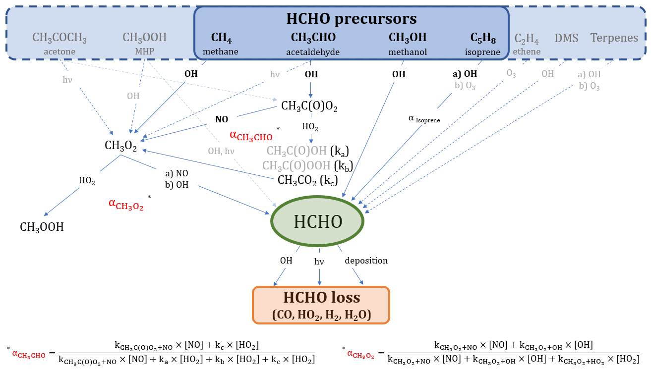
Figure 1Overview of the chemical and photolytic reactions which lead to HCHO production and loss, considering the trace gases measured during the CYPHEX field experiment. The black and bold font identifies the species which contribute mainly (∼80 %) to HCHO formation according to the findings in this study. For a better overview, we have omitted intermediate steps with a 100 % yield which are, instead, described in the main text.
Isoprene oxidation results in the formation of HCHO through the intermediate products methyl vinyl ketone and methacrolein, as described by Wolfe et al. (2016). The HCHO yield from isoprene (αIsoprene) is dependent on the ambient NO concentration and varies between around 30 % for low NOx and 60 % for high NOx (RO2 reacts primarily with NO; Atkinson et al., 2006; Palmer et al., 2003; Sumner et al., 2001). We calculate the HCHO yield via Eq. (3) and estimate [HO2] ≈ [RO2], as suggested by Sumner et al. (2001). This assumption is justified when looking at O3 production (P(O3)) terms. P(O3) can either be calculated via the photolytic reaction of NO2, as presented in Sect. 2.2, or via the reaction of HO2 or RO2 with NO. We equate the two terms, using the rate constant of the reaction of NO and CH3O2 as estimate for the reaction of NO and RO2, and calculate RO2. We show the diurnal profiles of HO2 and calculate RO2 in Fig. S1a in the Supplement. Conversely, we calculate P(O3) for both cases, equating RO2 to HO2, which show close agreement, and can be seen in Fig. S1b. This is also confirmed by findings from Crowley et al. (2018) (presented in Fig. 9), based on model simulations of HO2 and RO2 during HUMPPA. The yield can vary between 34 % (in the absence of NO) and 57 % (when NO chemistry dominates the fate of the RO2 formed), according to Eq. (3), which was originally determined experimentally by Miyoshi et al. (1994). We discuss the effects of the threshold values in Sect. 3.1. C5H8(OH)O2 is the peroxy radical resulting from isoprene oxidation and has six relevant isomers which can undergo multiple reactions yielding HCHO and many other products (Wennberg et al., 2018; Schwantes et al., 2020). Additionally, the formation of HCHO from isoprene does not occur instantaneously (as, for example, from methane or other VOC), but is likely time dependent. However, the consideration of this time-dependent formation and the detailed evaluation of the reactions paths from each peroxy radical isomer is beyond the scope of this study, and we, therefore, adapt the methodology presented by Sumner et al. (2001) to estimate the HCHO production from isoprene.
Methanol reacts with OH yielding HCHO via CH2OH and CH3O and following oxidation by O2 (Anderson et al., 2017; Stickler et al., 2006). Ethene is a precursor to HCHO through OH oxidation or ozonolysis (Alam et al., 2011; Atkinson et al., 2006). A potential source of HCHO in marine environments is dimethyl sulfide (DMS) via OH oxidation (Ayers et al., 1997; Urbanski et al., 1997). Terpenes, such as limonene or α-/β-pinene emitted from plants, can additionally be HCHO sources, as described by Lee et al. (2006).
Reactions (R1)–(R3) present the chemical loss processes of HCHO through OH oxidation and two different photolysis pathways. In addition, HCHO dry deposition – the uptake of HCHO by the Earth's surface – plays a role in HCHO loss, particularly during the night (Anderson et al., 2017; Possanzini et al., 2002; Sumner et al., 2001; Wesely and Hicks, 2000). While HCHO loss can also occur via wet deposition, as, for example, described by Seyfioglu et al. (2006), or via liquid-phase reactions in cloud droplets, as shown by Franco et al. (2021), this study investigates summertime campaigns without significant precipitation.
We will show in the scope of this work that reactions of methane, acetaldehyde, methanol and isoprene with OH almost completely account for HCHO production in the environments considered in this paper across Europe. We have highlighted these pathways in Fig. 1 in a black and bold font. Equations (4) and (5) show the calculation of the basic production P(HCHO)basic (compared to the reactions shown in Fig. 1) and the loss L(HCHO) terms. The k values represent the rate coefficients, j(HCHO) is the summed photolysis frequency for Reactions (R2) and (R3), vd describes the dry deposition velocity in centimeters per second (cm s−1) and BLH is the boundary layer height in centimeters.
Changes in the HCHO concentration are represented by Eq. (6), which include the production and loss from Eqs. (4)–(5), a transport term T(HCHO), such as advection or entrainment (can be positive or negative), and a term for primary emissions (Fischer et al., 2019).
2.2 O3 chemistry calculations
Figure 2 presents the main processes contributing to O3 formation and loss. The only significant chemical source of tropospheric O3 is the photolysis of nitrogen dioxide (NO2), which is converted to NO and O(3P) under the influence of sunlight. The reaction of O(3P) with molecular oxygen (O2) subsequently yields O3 (Jacob, 1999). NO2, in turn, is generated from the oxidation of NO by ozone or peroxy radicals (HO2 and RO2; Pusede et al., 2015).
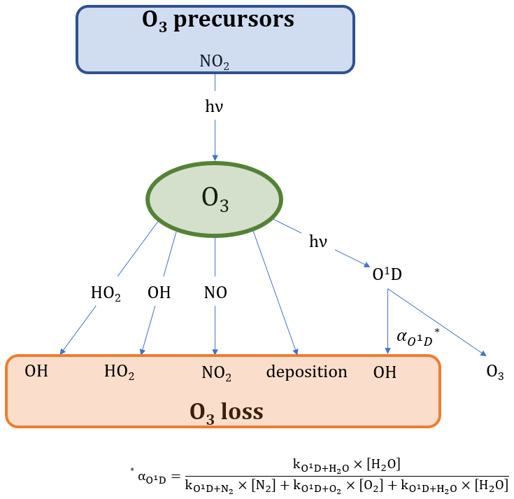
Figure 2Overview of the chemical and photolytic reactions which lead to O3 production and loss.
Ozone loss processes include the reaction with NO forming NO2, conversion with OH or HO2 to HO2 and OH, respectively, deposition processes and photolysis. O3 photolysis yields O(1D), which is deactivated to O(3P) (and then O3) via collision with nitrogen (N2) and oxygen (O2). O3 loss occurs when O(1D) reacts with water to form OH. The fraction of this reaction is presented by as shown in Eq. (7) (Bozem et al., 2017). The reaction of O3 and NO2 to form NO3 could potentially yield a net loss of O3 when being photolyzed back to NOx. However, only around 10 % of the NO3 photolysis leads to NO formation (which results in a O3 net loss; Stockwell and Calvert, 1983). Additionally, the reaction is likely negligible during the day, as O3 reacts much more rapidly with NO.
Equations (8) and (9) present the calculations for O3 production and loss.
As for HCHO, net changes in O3 are represented by production, loss and a transport term (either positive or negative), as shown in Eq. (10).
2.3 Field experiments
We have analyzed trace gases and further measurement parameters with regard to the HCHO and O3 budget at three different measurement sites across Europe, which are located in Cyprus (CYPHEX campaign, 2014), southern Germany (HOPE campaign, 2012) and Finland (HUMPPA campaign, 2010). Their geographic locations are shown in Fig. 3. We provide details on each campaign in the following sections. Please note that all times are in UTC (coordinated universal time). The time difference between 12:00 UTC and mean local noon is UTC+128 min for Cyprus, UTC+ 44 min for Germany and UTC+96 min for Finland (Fischer et al., 2019).
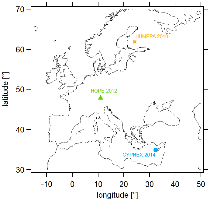
Figure 3Geographic locations of the measurement sites included in this analysis. CYPHEX – 34.96∘ N, 32.38∘ E, 650 (above sea level) and UTC+128 min (mean local time); HOPE – 47.80∘ N, 11.01∘ E, 980 and UTC+44 min; HUMPPA – 61.85∘ N, 24.28∘ E, 181 and UTC+96 min.
2.3.1 CYPHEX campaign in 2014
The Cyprus Photochemistry Experiment (CYPHEX) took place in Ineia, Cyprus, in July and August 2014. The measurement site was situated on a hilltop 650 (34.96∘ N, 32.38∘ E) in a remote location, with low population in the surrounding areas. The distance to the coastline of the Mediterranean Sea is approximately 10 km in the north and in the west. A detailed description of the measurement site can be found in Derstroff et al. (2017), Meusel et al. (2016) and Mallik et al. (2018). In this study, we consider the campaign days for which the trace gas measurements were available simultaneously, which is the time period 22–31 July 2014. NO and NO2 were measured via photolytic chemiluminescence (detector from ECO PHYSICS AG CLD 790 SR, Dürnten, Switzerland, and photolytic converter from Droplet Measurement Technologies, Boulder, CO, USA) with a total uncertainty of 20 % and 30 % and a detection limit of 5 and 20 pptv (parts per trillion by volume), respectively (Hosaynali Beygi et al., 2011; Tadic et al., 2020). O3 was measured via UV photometry (model 49 O3 analyzer, Thermo Environmental Instruments, USA) with a detection limit of 2 ppbv (parts per billion by volume) and a total uncertainty of 5 %. OH and HO2 were measured via laser-induced fluorescence spectroscopy with the custom-built HORUS (HydrOxyl Radical measurement Unit based on fluorescence Spectroscopy) instrument (accuracy of 28.5 % and 36 % and a detection limit of 1 × 10⁶ and 0.8 pptv, respectively; Marno et al., 2020; Novelli et al., 2014). HCHO was measured via the Hantzsch method with a commercial instrument (Aero-Laser GmbH, model AL 4021, Garmisch-Partenkirchen, Germany) with a detection limit of 38 pptv and a total uncertainty of 16 % (Kormann et al., 2003). C2H4 and CH4 were determined via gas chromatography flame ionization detection (GC 5000 VOC, AMA Instruments GmbH, Ulm, Germany). CH4 measurements had a detection limit of 20 ppbv and a total uncertainty of 2 %, and C2H4 measurements had a detection limit of 1–8 pptv and a total uncertainty of 10 % (Sobanski et al., 2016; Mallik et al., 2018). Isoprene was measured via gas chromatography mass spectrometry (MSD 5973, Agilent Technologies, Inc., Böblingen, Germany) with a detection limit of 1 pptv and a total uncertainty of 14.5 % (Derstroff et al., 2017). Oxygenated VOC (OVOC) was measured via proton transfer reaction time-of-flight mass spectrometry (PTR-TOF-MS; Ionicon Analytik GmbH, Innsbruck, Austria; CH3OH – 242 pptv limit of detection (LOD) and 37 % total uncertainty (TU); CH3COCH3 – 97 pptv LOD and 10 % TU; CH3CHO – 85 pptv LOD and 22 % TU; DMS – 18 pptv LOD and 12 % TU; the TU is 4 %–7 % higher for a relative humidity below 25 %; Veres et al., 2013; Graus et al., 2010). CH3OOH was measured via high-performance liquid chromatography with a detection limit of 25 pptv and a total uncertainty of 9 %. Photolysis frequencies were determined with a single monochromator spectral radiometer (Meteorologie Consult GmbH, Königstein, Germany) with a total uncertainty of around 10 %. The photolysis frequencies for acetaldehyde j(CH3CHO) and formaldehyde j(HCHO) were determined via parameterizations based on j(NO2) and j(O1D), according to Eq. (S1) in the Supplement, with the coefficients presented in Table S2. The latter were derived from least squares fits to photolysis frequencies from a large set of spectroradiometer measurements at Jülich, Germany (Bohn et al., 2008), under all weather conditions and were originally derived for the HUMPPA campaign. In this work, more recent quantum yields for the HCHO photolysis as recommended by IUPAC (2013) were used with an estimated uncertainty of 20 %. An example for the performance of the parameterization is shown in Fig. S2. An overview of all measured trace gases, including the measurement uncertainty and the time resolution of the data used in this study, can be found in Table S3. For the point-by-point calculations, the data were interpolated to the OH time stamp with a 4 min time resolution. All stated detection limits refer to the time resolution shown in Table S3.
2.3.2 HOPE campaign in 2012
The Hohenpeißenberg Photochemistry Experiment (HOPE) took place from June to September 2012 in Hohenpeißenberg, Germany at the Global Atmospheric Watch meteorological observatory (47.80∘ N, 11.01∘ E). The measurement location was situated on a hilltop, 980 , in a remote and vegetated area. More details on the campaign and the site location can be found in Novelli et al. (2017). O3, HCHO, OH and HO2 were measured with the same methods as described for the CYPHEX campaign in Sect. 2.3.1. NO and NO2 were measured via (photolysis) chemiluminescence by the German Weather Service, with an estimated uncertainty of 10 %. CH4 was measured via GC-FID (gas chromatography–flame ionization detector). Isoprene and OVOC were determined via a custom-built GC (Agilent Technologies, Inc.) FID/MS (mass spectrometry) system (Novelli et al., 2017; Werner et al., 2013). j(NO2) and j(O1D) were measured with filter radiometers (Meteorologie Consult GmbH, Königstein, Germany) with an uncertainty of 10 % (Bohn et al., 2008). j(HCHO) was determined via parameterization (Sect. 2.3.1). BLH (boundary layer height) measurements were not performed and instead adopted from Fischer et al. (2019), which are 1500 m for daytime (j(NO2) > 10−3 s−1) and 200 m for nighttime (j(NO2) < 10−3 s−1). These values were derived from BLH measurements at other locations during summertime, including the CYPHEX and the HUMPPA measurement site, and at a site in central Germany situated at a comparable altitude. We assume that this estimate increases the uncertainty from 20 % (BLH measurements) to 30 %. We determined the deposition velocity vd from the HCHO nighttime loss, as previously performed by Fischer et al. (2019), for H2O2. The loss rate coefficient kd was determined from the [HCHO] decrease from 21:00–01:30 UTC divided by the average HCHO concentration [HCHO]av during this time interval. Multiplication with the nighttime BLH (200 m) then yielded the deposition velocity according to Eq. (11). The HCHO loss via deposition during nighttime is independent of the BLH (see Eqs. 5 and 11).
Please note that vd derived this way represents a lower limit of the nighttime loss rate, as HCHO could be formed from NO3 and O3 chemistry (for example, from ozone and isoprene) at night (Crowley et al., 2018). The factor x considers the inconsistent mixing of the boundary layer at night, for which x was 2, assuming a linear gradient between the top and the bottom of the boundary layer. During the day, x equaled 1 (Shepson et al., 1992; Fischer et al., 2019). As we determined the loss rate from the nighttime decrease in HCHO, the daytime deposition velocity was twice the nighttime deposition velocity according to Eq. (11), which gives vd(day) = 0.94 cm s−1 and vd(night) = 0.47 cm s−1. Literature values for daytime deposition velocities range between 0.36 and 1.5 cm s−1 and for nighttime between 0.18 and 0.65 cm s−1 (Sumner et al., 2001; Stickler et al., 2007; DiGangi et al., 2011; Ayers et al., 1997). We, therefore, consider our calculation to yield reasonable estimates.
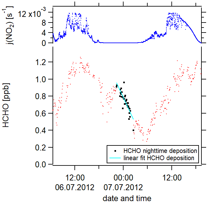
Figure 4The determination of the deposition velocity is based on the HCHO nighttime loss, which is here exemplarily shown for 1 night during the campaign HOPE (2012) in Hohenpeißenberg, southern Germany.
We have performed this calculation for 9 nights. Figure 4 exemplarily shows the nighttime loss of HCHO for 1 night during the HOPE campaign. Red data points represent the HCHO mixing ratios, the black color highlights the data points which we included in our analysis (nighttime HCHO loss) and the cyan line is the linear fit of these data points. An overview of the nights thus analyzed can be found in Fig. S3b. The uncertainty of each calculation results from the single uncertainties of , [HCHO]av and the nighttime BLH. The uncertainty of is composed of the HCHO measurement uncertainty (16 %) and the uncertainty of the fit (30 % upper limit) with the latter dominating. The uncertainty of [HCHO]av is based on the HCHO measurement uncertainty and the HCHO averaging (20 % upper limit). Again, the uncertainty of the averaging prevails over the measurement uncertainty. The uncertainty of the BLH is 30 %. Gaussian error propagation gives an overall uncertainty of from the calculation. Besides the uncertainty resulting from the calculation, an additional uncertainty arises from the atmospheric variability which describes ambient, instrumentally independent variations in the considered trace gases and parameters caused by, for example, atmospheric turbulence. The uncertainty from the atmospheric variability represented by the 1σ standard deviation of the mean over the considered 9 nights is 54 %, which exceeds the uncertainty from the calculation. We, therefore, estimate the uncertainty of vd to be 54 %. Please note that, in our uncertainty analysis, we consider the arising statistical errors but not the systematic errors which are not quantifiable but could potentially increase the overall uncertainty. An overview of all uncertainties and the time resolution of the measured trace gases can be found in Table S3. Absolute H2O concentrations were estimated from the measured relative humidity via the Magnus formula over water. Please note that some trace gases were not available simultaneously or only for a short overlap. We, therefore, present the averaged diurnal profiles.
2.3.3 HUMPPA campaign in 2010
The Hyytiälä United Measurements of Photochemistry and Particles (HUMPPA) campaign took place in July and August 2010 at SMEAR II (Station for Measuring Ecosystem–Atmosphere Relation) in Hyytiälä, Finland (61.85∘ N, 24.28∘ E, 181 ). The site is located in a remote area in a boreal forest. A detailed description of the campaign can be found in Williams et al. (2011). The measurement methods for NOx, O3, HCHO and CH4 were the same as those presented for the CYPHEX campaign. CH3OH was measured via a cold trap PTR-MS with a detection limit of around 50 pptv (integration time of 5 min). Acetaldehyde was measured via PTR-MS with a detection limit of 50 pptv (integration time of 6 min; Williams et al., 2011). Isoprene was measured via GC (GC 6890A, Agilent Technologies, Inc.) coupled to a mass selective detector (MSD 5973 inert, Agilent Technologies, Inc.) with an uncertainty of around 15 %. Highly constrained box model simulations, which were in fair agreement with experimental data, were available for OH and HO2, as described by Crowley et al. (2018), with an uncertainty in the order of 30 %–40 %. j(NO2) and j(O1D) were measured with filter radiometers (Meteorologie Consult GmbH, Königstein, Germany) with an uncertainty of around 10 %; j(HCHO) was determined via parameterization (analogous to CYPHEX and HOPE). H2O was measured with an infrared light absorption analyzer (URAS 4 H2O, Hartmann & Braun AG, Frankfurt am Main, Germany). The BLH was measured by radio soundings, as presented by Ouwersloot et al. (2012), ranging from 200 m during nighttime (here j(NO2) < 10−3 s−1) to 1500 m during daytime (here j(NO2) < 10−3 s−1; Fischer et al., 2019). The deposition velocity was determined analogously to the HOPE campaign, based on the nighttime HCHO loss on the basis of 14 nights, and was 0.85 cm s−1 during the day and 0.43 cm s−1 during the night. The uncertainty of the calculation results from the single uncertainties of (16 %), [HCHO]av (33 %) and the nighttime BLH (20 %). Gaussian error propagation gives an overall uncertainty of 42 % from the calculation. The atmospheric variability equals 54 %. We, therefore, estimate the total uncertainty of the deposition velocity to be 54 %. An overview of all considered nights and the respective HCHO loss is presented in Fig. S3c. The deposition velocity of ozone was adopted from Rannik et al. (2012) for the time period during calendar weeks 25–34 of the year and a relative humidity below 70 %, which is 0.491 cm s−1 for daytime and 0.069 cm s−1 for nighttime. A modeling study by Emmerichs et al. (2021) presents the average values in the same order of magnitude (∼ 0.2–0.3 cm s−1 for July and August). Again, uncertainties and time resolution are shown in Table S3. Similar to the HOPE campaign, some trace gases were not available simultaneously, and we, therefore, present the averaged diurnal profiles.
3.1 Net HCHO production during CYPHEX in 2014
HCHO concentrations during the CYPHEX campaign ranged between 0.3 and 1.9 ppbv (1.1 ± 0.4 ppbv on average), with a maximum in the diel cycle during morning hours (04:00 UTC) and a minimum in the afternoon (15:00 UTC). Please note the mean local time difference stated in Sect. 2.3 and Fig. 3. The temporal development of HCHO concentrations during the campaign and the respective j(NO2) values (to illustrate the daily cycle) are shown in Fig. S3a. Figure S4a presents the diurnal average of HCHO, including its rate of change . The uncertainty is dominated by the atmospheric variability which is on average 27 % for daytime HCHO.
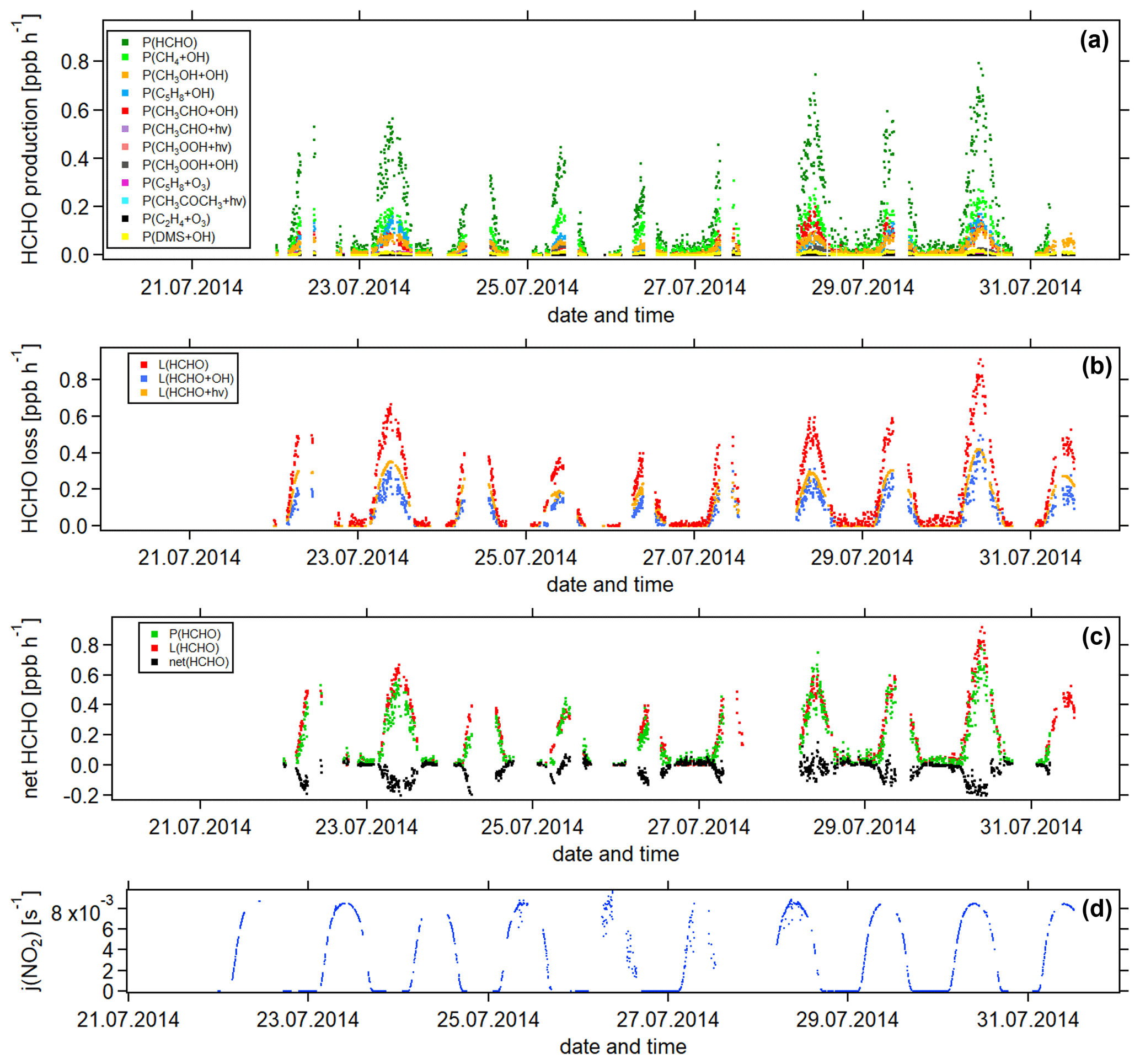
Figure 5Temporal development of (a) HCHO production terms, (b) HCHO loss terms and (c) net HCHO from 22 July to 31 July 2014 during the CYPHEX research campaign in Cyprus. The NO2 photolysis frequency j(NO2) is shown in panel (d) as an illustration of the diurnal cycle. All times are in UTC.
Figure 5 shows the time series of the HCHO production terms (Fig. 5a), the HCHO loss terms (Fig. 5b) and the net HCHO production (Fig. 5c) during the CYPHEX research campaign in Cyprus in July 2014. We calculated the HCHO production terms for all measured gas-phase precursors shown in Fig. 1. The individual production terms are shown in Fig. S5. The total measurement uncertainties were determined via Gaussian error propagation and were 28 % for HCHO production (31 % for only considering the OH oxidation of methane, methanol, isoprene and acetaldehyde) and 26 % for HCHO loss. Table S4 provides an overview of all calculated uncertainties. We present two example step-by-step calculations via Gaussian error propagation in Eqs. (S2)–(S8). All other calculations were made accordingly. We have neglected the uncertainties for the HCHO yield from isoprene, and and instead present a sensitivity study for these parameters later in this section. Dark green colors show the overall HCHO production as the sum of all single production terms. All production terms show a diurnal cycle which follows the course of the photolysis frequency j(NO2), which we show in Fig. 5d. Photolysis reactions do not take place after sunset, and oxidation reactions are dependent on the abundance of OH radicals, which is low during nighttime. Therefore, HCHO production approaches zero during nighttime. Due to data gaps, a full diurnal profile was only available for 23, 28 and 30 July, where the overall HCHO production reached maxima between 0.6 and 0.8 ppbv h−1. The reactions of methane, methanol, isoprene and acetaldehyde with OH dominated the HCHO production processes. This is additionally illustrated in Fig. 6, which presents the daily average share (including day- and nighttime values) of each production term based on a balance to the overall loss rate. HCHO production was, therefore, dominated by the reaction of methane and OH (almost a third), followed by the oxidation of acetaldehyde contributing around 15 % and the OH oxidations of isoprene and methanol, both contributing around 14 %. These four species together represented 75 % of the overall HCHO production required to balance the sinks. The production through the OH oxidation of methyl hydroperoxide and dimethyl sulfide and through the reaction of isoprene and ozone contributed by around 1 %–2 % each. The remaining species each yielded less than 1 % of the overall HCHO. Less than 20 % was unaccounted for (the rest in Fig. 6). This part also includes HCHO production from terpenes via oxidation through OH or O3. The yields from these reactions vary greatly in the literature. Considering the yields from OH oxidation, suggested by Lee et al. (2006), from laboratory investigations, limonene, β- and α-pinene would account for 3 %, 2 % and 1 % of the overall HCHO production, respectively. The isoprene yield is limited to a value between 34 % and 57 %. The lower limit would give a HCHO production from isoprene of 11 %, and the upper limit would yield 19 %. The value for can theoretically be between 0 % and 100 % but is likely situated at the upper end due to the availability of NO. As an example, a 20 % decrease in would give a HCHO production from CH3O2 of 38 % (compared to 47 % for the calculated ). A 20 % increase would yield 57 % on average and decrease the rest to less than 10 %. For , a 20 % decrease and increase would give a HCHO yield from acetaldehyde of 12 % and 18 %, respectively, assuming a constant . Please note that the uncertainty of the absolute values used to create this pie chart is dominated by the atmospheric and diurnal variability in the single terms and is of the order of 100 %.

Figure 6Chemical production terms of HCHO during CYPHEX, including daily averages of all data.
HCHO loss was determined from the reaction with OH and photolysis. Red colors in Fig. 5b show the overall calculated HCHO loss. Similar to the HCHO production, HCHO loss via OH and photolysis only plays a role during the daytime. At night, dry deposition is the only HCHO loss mechanism, and the deposition velocity vd can be determined from the nighttime decrease in ambient HCHO concentrations, as shown by Sumner et al. (2001). However, we often observed increasing HCHO concentrations during nighttime, particularly before sunrise. The reason for this nighttime HCHO increase is not yet fully understood. The role of the deposition processes at elevated altitudes is not yet fully understood but is likely influenced by flows along mountain slopes and horizontal advection on hilltops. For hilltops, incoming air through advection likely originated from areas without deposition (too high above the ground; Derstroff et al., 2017). Please note that the effect of deposition processes could also be counteracted by a nighttime HCHO source, such as terpene oxidation by ozone or advection. The determined value for the deposition can, therefore, be seen as being a lower estimate (Crowley et al., 2018). As we do not observe the net loss of HCHO at night during the CYPHEX campaign, we estimate the dry deposition to be negligible. Figure 5c shows the overall HCHO production and loss rates, as well as the difference between both, which we refer to as net HCHO production, in black. Production and loss showed a good balance with values of ± 0.2 ppbv h−1. On most days, HCHO loss prevailed over HCHO production, based on measured precursors.
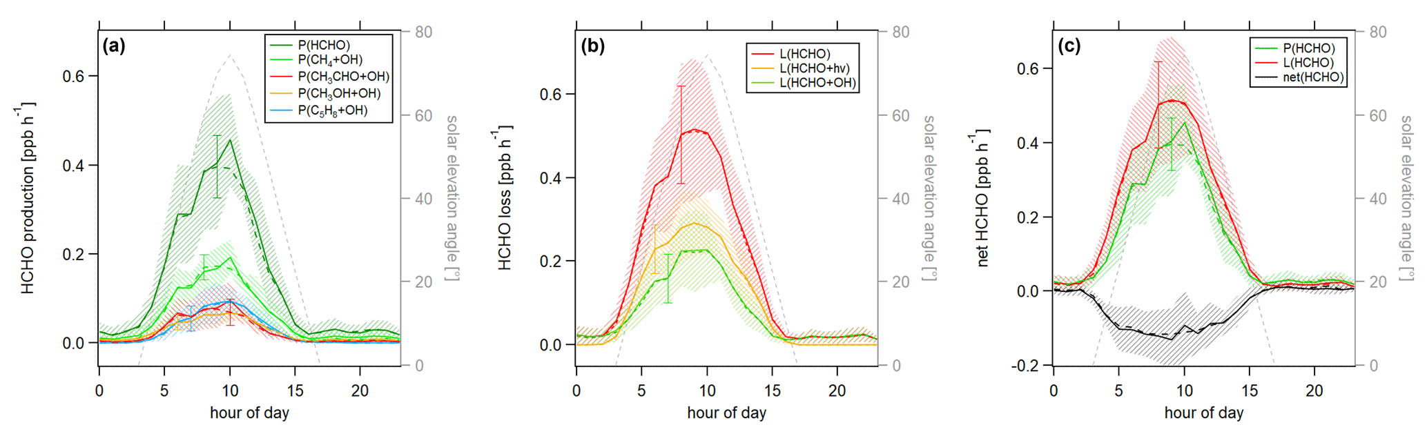
Figure 7Diurnal profiles of (a) HCHO production P(HCHO), (b) HCHO loss L(HCHO) and (c) HCHO net terms during the CYPHEX campaign in 2014. Solid lines show the hourly averaged HCHO production and loss terms, based on the point-by-point calculation of simultaneous parameter measurements. The uncertainty from the atmospheric variability is represented by the 1σ error shades. For the dashed lines, all measurement parameters were averaged first, followed by the calculation of hourly HCHO production and loss terms. The uncertainty is based on the atmospheric variability of all parameters and is exemplarily shown by the error bar for one point for each production and loss term. The gray dashed line represents the diurnal solar elevation angle at the measurement site, as determined by help of the NOAA Solar Calculator (2021).
In order to better account for diurnal changes, we investigated the daily cycle of HCHO production and loss rates based on hourly averages over all measurement days. Figure 7 shows the diurnal profiles of the main HCHO production terms (Fig. 7a) as determined above, the HCHO loss terms (Fig. 7b) and net HCHO production (Fig. 7c). The solid lines represent the hourly averages of the point-by-point calculation of the production and loss terms. The uncertainty is composed of the measurement uncertainty and the atmospheric variability, where the latter is demonstrated by the 1σ error shades. For HCHO production, the measurement uncertainty was 31 %, and the daytime atmospheric variability was 40 % (61 % for day and night). For HCHO loss, the uncertainties were 26 % and 34 % (57 %), respectively. In both cases, the overall uncertainty was dominated by the atmospheric variability. The dashed lines show the hourly production and loss terms calculated from the hourly averaged trace gas concentrations. The uncertainty from the atmospheric variability was 22 % (34 %) for HCHO production and 25 % (52 %) for HCHO loss and is exemplarily indicated by an error bar for one point for each production and loss term in Fig. 7. Both methods have advantages and disadvantages. The point-by-point calculation allows for a simultaneous consideration of all measurement parameters. Potential atmospheric changes or incidents such as wind, precipitation or rare primary emission events are reflected by all parameters as they are monitored at the same time. On the other hand, this method reduces the number of data points used as only one single missing species prevents the calculation of the overall term. In order to increase the number of results, we have interpolated the values for the isoprene yield (data coverage 81 %), and (data coverage 64 %). Calculating production and loss terms from the hourly averaged trace gas concentrations allows for the inclusion of all measured parameters but could potentially increase the uncertainty of the estimate, depending on the duration and overlap of the single measurements. However, in this case, the data were limited to 1 week in July with mainly simultaneous measurements of all parameters, and we, therefore, do not expect large uncertainties. The similarity of the results, as shown in Fig. 7, indicates that both methods provide reasonable results.
For HCHO production, the daily maxima of around 0.4–0.45 ppbv h−1 were reached between 09:00 and 10:00 UTC, which was coincident with the maximum of the photolysis frequency j(NO2). HCHO production from methane dominated the overall production term, with a maximum of close to 0.2 ppbv h−1, followed by acetaldehyde, isoprene and methanol. HCHO loss peaked around 09:00 UTC, with a value of 0.5 ppbv h−1, with around 55 % contribution from photolysis and 45 % from OH oxidation. Figure 7c shows that the calculated production term for HCHO can almost completely balance the loss, which, assuming that the major loss processes are well constrained, leads to the conclusion that HCHO production can be approximated by OH oxidation of methane, acetaldehyde, isoprene and methanol. This is in line with the HCHO rate of change presented in Fig. S4a which oscillated around zero. Therefore, transport processes and primary emissions during CYPHEX can likely be excluded.
3.2 Net O3 production during CYPHEX in 2014
Ozone varied between 46 and 104 ppbv during the CYPHEX campaign (70 ± 13 ppbv on average), with a diel maximum at 04:00 UTC and a minimum at 15:00 UTC. The time series of O3 concentrations is presented in Fig. S6a. The diel mean, including the rate of change , can be found in Fig. S7a. The uncertainty is dominated by the atmospheric variability, which is on average 16 % (1σ) for O3.
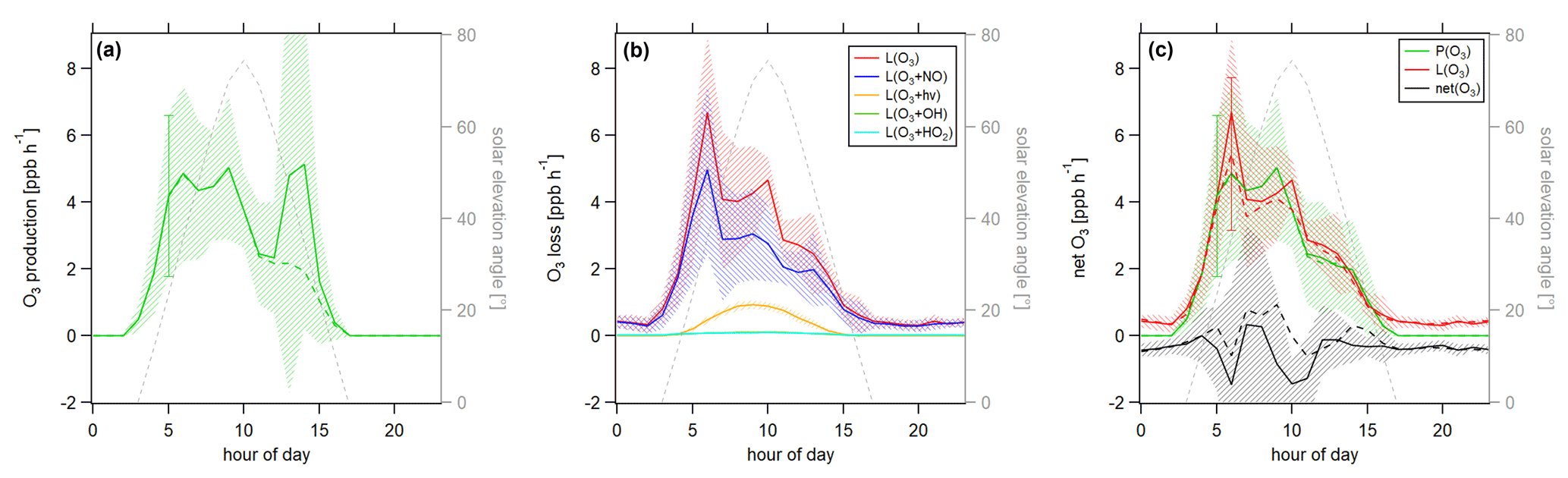
Figure 8Diurnal profiles of (a) ozone production P(O3), (b) ozone loss L(O3) and (c) ozone net terms during the CYPHEX campaign in 2014. Solid lines show the hourly averaged O3 production and loss terms, based on the point-by-point calculation of simultaneous parameter measurements. The uncertainty from the atmospheric variability is represented by the 1σ error shades. For the dashed lines, all measurement parameters were averaged first, followed by the calculation of hourly O3 production and loss terms. The uncertainty is mostly dominated by the atmospheric variability in all parameters and is exemplarily shown by the error bar for one point for each production and loss term. Please find the temporal development of production and loss terms throughout the campaign in Fig. S8.
Figure 8 shows the diurnal cycle of the production and loss rates for ozone, analogous to Fig. 7. Solid lines show the hourly averaged point-by-point calculations of the O3 production and loss terms. The 1σ error shades present the atmospheric variability, which was 59 % for O3 production and 37 % for O3 daytime loss (44 % for day and night). The measurement uncertainties were 32 % and 16 %, respectively, and the overall uncertainty was, therefore, dominated by the atmospheric variability. Dashed lines show the O3 production and loss terms based on the hourly averaged measurement parameters. The uncertainty resulting from the averaging of the individual parameters is exemplarily shown by the error bar for one point and is similar to the atmospheric variability obtained by the point-by-point method (57 % for P(O3) and 35 % (49 %) for L(O3)). Figure 8a shows O3 production represented by the photolysis of NO2. Figure 8b shows the O3 loss terms. O3 loss through reaction with NO was dominant, followed by photolysis. The loss via OH and HO2 was negligibly small. O3 net production during the CYPHEX campaign was, therefore, clearly dominated by nitrogen oxides chemistry. Figure 8c shows the net O3 production. O3 production and loss were similar throughout the day, with peak values of 4–7 ppbv h−1 between 05:00 and 10:00 UTC. Net O3 production was between −1 and 1 ppbv h−1. Please note that we have excluded the NO2 data from 24 July between 13:15 and 16:15 UTC due to a singular high-concentration event. The large spike in NO2 (O3 titration of NO) is likely the result of sampling air impacted by the exhaust from a diesel generator which provided on-site power and was located about 200 m from the containers housing the instruments. We show O3 net production, including all NO2 data points, in Fig. S9a. O3 production is directly proportional to the NO2 concentration, according to Eq. (8), which explains the large afternoon production peak. We show the diel profile of NO2 concentrations with and without the afternoon peak in Fig. S9b. Production and loss terms for O3 were balanced, and the O3 rate of change oscillated around zero (Fig. S7a), suggesting that the diel variability was likely not impacted by transport processes.
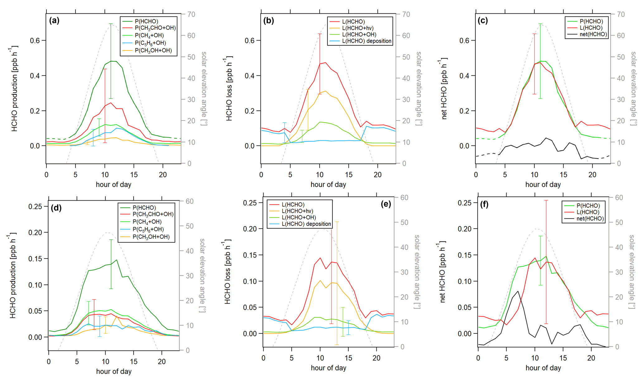
Figure 9Diurnal profiles of HCHO production P(HCHO) and loss L(HCHO) terms during the HOPE campaign 2012 (top row) and the HUMPPA campaign 2010 (bottom row). (a) P(HCHO), (b) L(HCHO), (c) net HCHO), (d) P(HCHO), (e) L(HCHO) and (f) net(HCHO).
3.3 Comparison with HOPE (2012) and HUMPPA (2010)
3.3.1 Net HCHO production
We have shown, in Sect. 3.1 and 3.2, that the hourly averaging of measurement parameters and subsequent calculation of production and loss terms yielded reliable results during the CYPHEX campaign. For HUMPPA and HOPE, we have pursued this approach regarding the calculations of HCHO and O3 production and loss terms, as the simultaneous data availability for all measurement parameters was too low for a point-by-point analysis.
HCHO mixing ratios during the HOPE campaign varied between 0.1 and 3.2 ppbv (1.1 ± 0.5 ppbv on average), with a maximum in the diel cycle at 15:00 UTC and a minimum at 06:00 UTC. The average mixing ratio was similar to the average mixing ratio during the CYPHEX campaign, but the variability was higher, which is likely due to the longer time period of available data which was about 4 weeks for HOPE (compared to a bit more than 1 week for CYPHEX), including, e.g., larger temperature variations. HCHO mixing ratios in Hyytiälä during the HUMPPA campaign ranged between 0.03 and 5.7 ppbv, with an average of 0.4 ± 0.5 ppbv. The variability is high because of biomass burning events in Russia which were detected at the site in Finland on 26–30 July and 9 August, as described by Williams et al. (2011). The large HCHO peaks detected on these days can also be seen in Fig. S3c. Figure S4b and c present the diurnal cycles for HCHO, including the rate of change during HOPE and HUMPPA. The uncertainty is dominated by the atmospheric variability represented by the 1σ standard deviation, which is, on average, 44 % for HCHO for HOPE and 106 % for HUMPPA.
Figure 9 shows the HCHO production and loss rates for the two campaigns. For all cases, the uncertainty was dominated by the atmospheric variability (1σ), which was 42 % for daytime HCHO production and 40 % for daytime HCHO loss in Hohenpeißenberg and 38 % and 77 % in Hyytiälä, respectively. The measurement uncertainty was around 30 % to 40 %. We present the atmospheric variability with the error bars in Fig. 9. For better clarity, we only show one error bar for each term. An overview of all calculated uncertainties can be found in Table S4. HCHO production during HOPE is shown in Fig. 9a. The maximum production rate of 0.48 ppbv h−1 was reached between 11:00 and 12:00 UTC, and a comparison to j(NO2) shows good agreement with local noon. The production of HCHO was dominated by the oxidation of acetaldehyde, which contributed to the peak production by around 50 %, followed by methane, isoprene and methanol. We show a pie chart representing the contribution of the single HCHO production terms during HOPE in Fig. S10a. HCHO loss is shown in Fig. 9b. The maximum loss rate of HCHO was 0.46 ppbv h−1. During the day, HCHO loss was dominated by photolysis and oxidation, while, at nighttime, deposition was the main loss path for formaldehyde in Hohenpeißenberg. Figure 9c shows HCHO net production during HOPE. The calculated production of HCHO slightly prevailed over its loss. At 11:00 UTC, HCHO loss was > 95 % of HCHO production. Overall absolute loss and production terms were very similar compared to the results obtained for the site in Cyprus. The main difference is the composition of the HCHO production, which was dominated by the oxidation of acetaldehyde in Hohenpeißenberg and by the oxidation of methane in Cyprus. HCHO production and loss during the HUMPPA campaign are shown in Fig. 9d–f. HCHO production reached a peak value of 0.15 ppbv h−1 at 12:00 UTC. Methane and acetaldehyde contributed to the overall production by approximately equal parts, followed by isoprene and methanol. Figure S10b shows the share of the individual HCHO production terms during HUMPPA. Axinte (2016) showed that the contribution from terpene oxidation to HCHO production was small (1 %–2 % each), which is in line with our findings for the CYPHEX campaign. HCHO loss was dominated by photolysis during the day and by dry deposition at night. Figure 9f shows that HCHO production and loss were in good agreement throughout the day (∼ 90 %), apart from the morning hours 06:00–07:00 UTC when HCHO production prevailed over its loss by around 2 to 3 times, indicating a missing loss term, most likely due to dilution with HCHO-poor air during the rise of the planetary boundary layer in the early morning hours (accompanied by a peak in the HCHO rate of change as shown in Fig. S4b). Overall production and loss terms for HCHO were around 3 times smaller compared to the values obtained for the sites in Germany and Cyprus. We also observed smaller concentrations of CH4, OH radicals and HCHO. It is notable that HCHO production was slightly higher than the loss for both the HUMPPA and the HOPE campaign. This is also reflected by peaks in the rate of change (0.1–0.2 ppbv h−1) in the morning/midday hours (Fig. S4b and c) and could indicate a transport effect from areas with lower HCHO concentration, e.g., entrainment, according to Eq. (6). For HUMPPA, this idea is supported when excluding the data impacted by biomass burning, which we show in Fig. S11a. It can be seen that HCHO production prevailed over its loss, suggesting a missing loss term. The difference was highest in the morning hours, with approximately 0.1 ppbv h−1, and decreased throughout the day indicating, e.g., a vertical dilution from higher, HCHO-poor altitudes. For comparison, Fig. S11b shows the HCHO production and loss terms when only considering data impacted by biomass burning. Due to high HCHO mixing ratios, the loss terms were substantially higher compared to its production. In periods influenced by biomass burning, the highest HCHO yield was from acetaldehyde (averaged diel mixing ratios of 1.1 ppbv compared to 0.6 ppbv without biomass burning); when excluding biomass burning, the yield from methane was slightly higher.
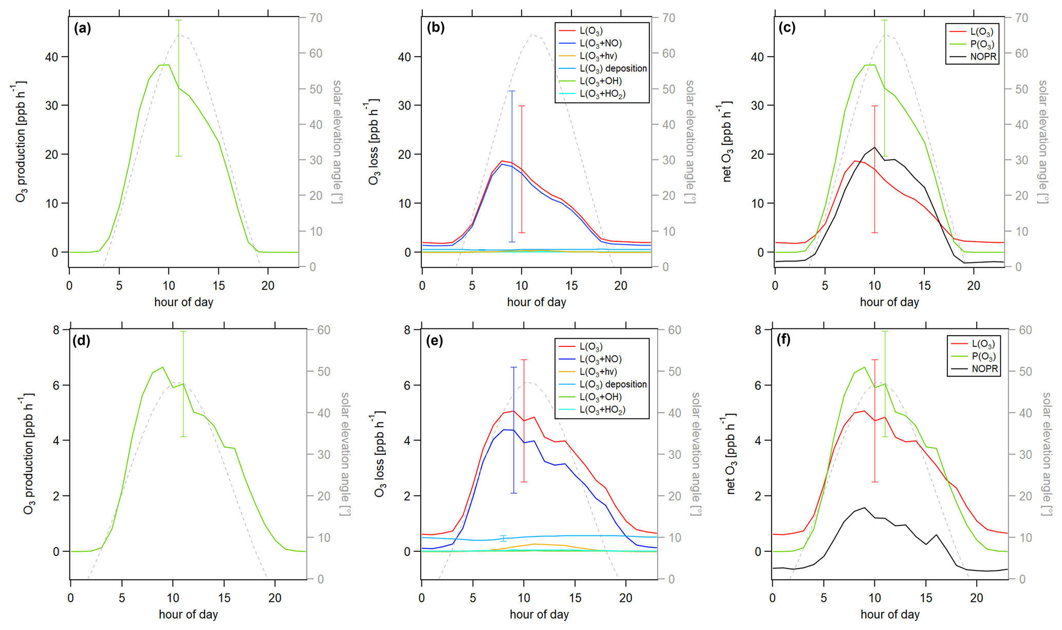
Figure 10Diurnal profiles of O3 production P(O3) and loss L(O3) terms during the HOPE campaign 2012 (top row) and the HUMPPA campaign 2010 (bottom row). (a) P(O3), (b) L(O3), (c) net O3, (d) P(O3), (e) L(O3) and (f) net(O3).
3.3.2 Net O3 production
Ozone concentrations in Hohenpeißenberg were, on average, 44 ± 11 ppbv, with a minimum of 5 ppbv and a maximum of 97 ppbv. The campaign-averaged diel profile displayed a peak of 48 ppbv at 16:00 UTC and a minimum of 39 ppbv at 07:00 UTC. In Hyytiälä, ozone concentrations were between 20 and 76 ppbv and 42 ± 11 ppbv on average. A diel peak of 49 ppbv was reached between 15:00 and 16:00 UTC and a minimum of 34 ppbv at 05:00 UTC. The temporal development of ozone concentrations during the campaigns and the diurnal averages can be found in Figs. S6 and S7. The uncertainty is dominated by the atmospheric variability (1σ) which is, on average, 24 % for O3 for HOPE and 23 % for HUMPPA.
Figure 10 shows the ozone production and loss terms for the research campaigns HOPE and HUMPPA. The overall uncertainty was again dominated by the atmospheric variability (1σ), which was 58 % for the daytime O3 production and 90 % for the daytime O3 loss in Hohenpeißenberg and 44 % and 51 %, respectively, in Hyytiälä. In comparison, the measurement uncertainty regarding overall production and loss was between 10 % and 15 %. A detailed overview of the uncertainties can be found in Table S4. We adopted the dry deposition velocity for ozone in Hyytiälä from Rannik et al. (2012). No literature values for the ozone dry deposition in Hohenpeißenberg were available. Therefore, we applied the same values as for the HUMPPA campaign, which increased the uncertainty of the analysis. However, the fraction of ozone dry deposition of the overall loss was small. For the applied deposition velocity, dry deposition contributed by around 4 % during the daytime. For a change in vd of ± 100 %, the fraction varied between 2 % and 7 %. We, therefore, assume a maximum additional uncertainty of 5 % resulting from this estimate. Ozone production in Hohenpeißenberg reached peak values of 38 ppbv h−1. In contrast, ozone loss showed a maximum of only 21 ppbv h−1, most of which was due to the reaction with NO. In Hyytiälä, ozone production was 6.7 ppbv h−1 at its diurnal maximum, while ozone loss reached 5.1 ppbv h−1 and was mainly composed of the loss via NO, followed by dry deposition. The differences between production and loss terms could again indicate a transport effect, according to Eq. (10), as described for HCHO. The rate of change for O3 showed peak values (2–3 ppbv h−1) during the morning/midday hours, which was not observed for the CYPHEX campaign (Fig. S7). O3 production and loss terms during HUMPPA and CYPHEX were similar, while the values were significantly higher during HOPE. O3 production in Hohenpeißenberg was almost 1 order of magnitude higher compared to the other sites, which was likely due to the higher ambient NOx concentrations. The net O3 production (the difference between O3 production and loss) at each site could give a hint regarding the dominant chemical ozone regime. For HOPE, net O3 production was significantly above zero, with diurnal maximum values of around 20 ppb h−1 at 10:00 UTC, which could indicate a VOC limitation. In contrast, net O3 production was close to zero for CYPHEX, and the ozone regime was more likely NOx limited. We will discuss the dominant chemical ozone regime in detail in the following section.
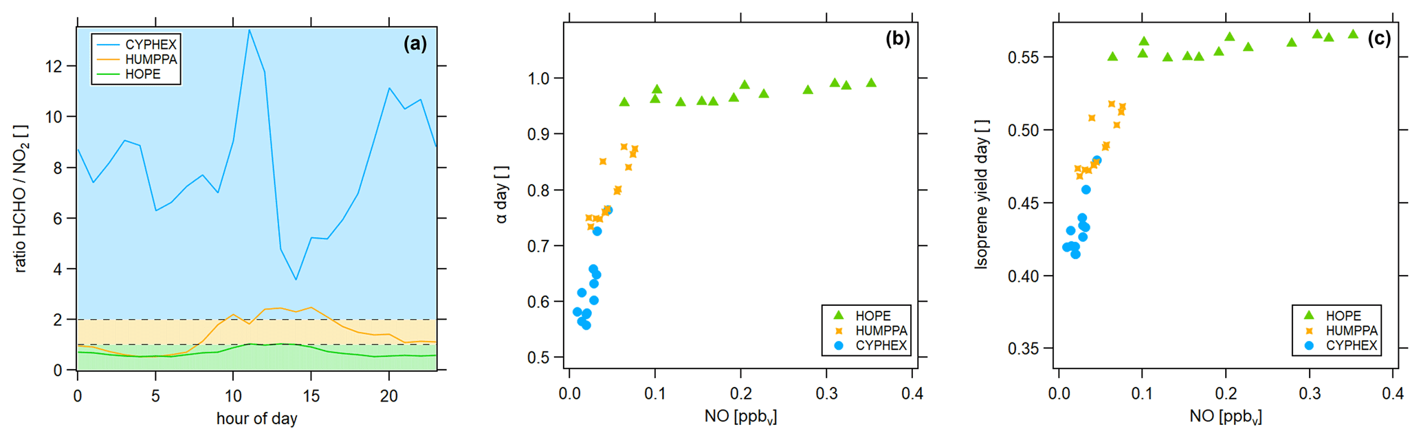
Figure 11Determination of the dominant chemical regime via (a) the ratio (colored areas indicate the dominant chemical regime, according to Duncan et al. (2010), which are blue ( > 2) for a NOx limitation, green ( < 1) for a VOC limitation and yellow (1 < < 2) for the transition), (b) the fraction of methyl peroxy radicals forming HCHO and (c) the HCHO yield from isoprene.
3.4 Chemical regime
Various methods exist to determine the prevailing chemical ozone regime (i.e., the net efficiency of production or loss), one of which is the ratio of formaldehyde and nitrogen dioxide. We have calculated the diel ratios for all three measurement sites, which is shown in Fig. 11a. The ratio was highest in Cyprus with 8.0 ± 2.4, followed by 1.4 ± 0.7 in Hyytiälä and 0.7 ± 0.2 in Hohenpeißenberg. According to findings by Martin et al. (2004) and Duncan et al. (2010) these values indicate a dominant NOx-limited regime during CYPHEX and a dominant VOC-limited regime during HOPE. The regime during HUMPPA was likely transitioning between both limitations. We show two additional approaches for determining the present chemical regime in Fig. 11. In Fig. 11b, we present the daytime averages of versus the NO concentration. All campaigns show a linear correlation. Daytime average NO concentrations during CYPHEX ranged from 1 to 45 pptv, accompanied by an increase in from around 55 % to 75 %, giving a slope of 5.54 ppbv−1. The slope for the increase in with NO is approximately half for the HUMPPA campaign, with a value of 2.52 ppbv−1. The NO concentration ranged from 22 to 76 pptv, along with an increase in from 73 % to 87 %. Finally, for the HOPE campaign, NO concentrations and its range were highest with values between 60 and 350 pptv. At the same time, showed the smallest increase by only 3 percentage points. The resulting slope was the smallest, with a value of 0.11 ppbv−1. indicates the share of CH3O2 that forms HCHO, predominantly through the reaction with NO. The competing reaction is the conversion with HO2 to CH3OOH. A high value for , which is not (or only a little) responsive to a changing NO concentration, indicates a VOC limited regime, while in a NOx-limited regime, small changes in ambient NO have a large effect on the HCHO formation from CH3O2. Analogously, we show the HCHO yield from isoprene, according to Eq. (3), versus NO concentrations in Fig. 11c, which we suggest as an indicator for the present chemical regime too. For the CYPHEX campaign, the isoprene yield was most responsive to ambient NO concentrations with a slope of 1.61 ppbv−1, indicating a NOx limitation. In contrast, the isoprene yield during the HOPE campaign was almost non-responsive to changing NO, indicating a VOC limitation (slope of 0.05 ppbv−1). Although specialized instrumentation is still necessary to measure NO, OH and HO2, these methods to determine the dominant chemical regime only require the knowledge of a small number of trace gas concentrations and the ambient temperature.
In this study, we have analyzed the photochemical processes contributing to formaldehyde and ozone production and loss across Europe based on in situ trace gas observations during three different stationary field campaigns in Cyprus (CYPHEX in 2014), Germany (HOPE in 2012) and Finland (HUMPPA in 2010). Very consistently across all sites, we found that formaldehyde loss can be predominantly accounted for by the production via the OH oxidation of methane, acetaldehyde, isoprene and methanol. Formaldehyde loss is represented by photolysis, OH oxidation and, to a small extent, by dry deposition. Ozone chemistry is mainly controlled by nitrogen oxides. The production can be described by NO2 photolysis, and the loss is mainly a function of NO reduction and, to a smaller extent, of photolysis and dry deposition. We found a good agreement between O3 production and loss in Cyprus and Finland, while the production was approximately double its loss in southern Germany. Finally, we have presented several different approaches for determining the prevalent chemical regime, which included the ratio, and the fraction of CH3O2 forming HCHO, and the HCHO yield from isoprene in its dependence on the ambient NO concentration. We identify a VOC-limited regime during the HOPE campaign in Germany and a NOx-limited regime during the CYPHEX campaign in Cyprus, whereas chemistry during the HUMPPA campaign in Finland was likely at a transitional point.
While ongoing research on HCHO photochemical processes has continuously widened the contributors to possible production paths and the complexity of calculations and models, we show that the consideration of only four precursor VOCs is capable of almost completely representing the HCHO production term at various sites across Europe. We encourage extending the HCHO budget calculations based on in situ trace gas observations to more sites worldwide as a simple, but effective, tool to monitor photochemical processes and air quality, including the dominant chemical regime.
All data generated and analyzed for this study are available from KEEPER (2021; https://keeper.mpdl.mpg.de/, last access: 6 December 2021) upon request to the authors.
The supplement related to this article is available online at: https://doi.org/10.5194/acp-21-18413-2021-supplement.
HF had the idea. CMN and HF designed the study. CMN analyzed the data and wrote the paper. JS, JNC and BB provided J values. CPD provided trace gas measurements for HOPE. JNC provided OH and HO2 model data for HUMPPA. JW provided VOC data. HH, CE, AN, KT, MM, CM and LT provided OH and HO2 data for CYPHEX and HOPE. HCHO data were measured and provided by AR and RA. SH provided CH3OOH data. NOx and O3 data were obtained from HF. JL significantly contributed to planning the research campaigns.
The contact author has declared that neither they nor their co-authors have any competing interests.
Publisher's note: Copernicus Publications remains neutral with regard to jurisdictional claims in published maps and institutional affiliations.
We acknowledge all researchers and supporting personnel who participated in the CYPHEX campaign in 2014, the HOPE campaign in 2012 and the HUMPPA campaign in 2010. We would like to thank Pekka Rantala (University of Helsinki), for providing the CH3CHO data for HUMPPA. This work was supported by the Max Planck Graduate Center with the Johannes Gutenberg-Universität Mainz (MPGC).
The article processing charges for this open-access publication were covered by the Max Planck Society.
This paper was edited by John Liggio and reviewed by two anonymous referees.
Alam, M. S., Camredon, M., Rickard, A. R., Carr, T., Wyche, K. P., Hornsby, K. E., Monks, P. S., and Bloss, W. J.: Total radical yields from tropospheric ethene ozonolysis, Phys. Chem. Chem. Phys., 13, 11002–11015, https://doi.org/10.1039/C0CP02342F, 2011. a
Anderson, D., Nicely, J., Wolfe, G., Hanisco, T., Salawitch, R., Canty, T., Dickerson, R., Apel, E., Baidar, S., Bannan, T., Blake, N. J., Chen, D., Dix, B., Fernandez, R. P., Hall, S. R., Hornbrook, R. S., Huey, L. G., Josse, B., Jöckel, P., Kinnison, D. E., Koenig, T. K., Breton, M. L., Marécal, V., Morgenstern, O., Oman, L. D., Pan, L. L., Percival, C., Plummer, D., Revell, L. E., Rozanov, E., Saiz-Lopez, A., Stenke, A., Sudo, K., Tilmes, S., Ullmann, K., Volkamer, R., Weinheimer, A. J., and Zeng, G.: Formaldehyde in the tropical western Pacific: Chemical sources and sinks, convective transport, and representation in CAM-Chem and the CCMI models, J. Geophys. Res.-Atmos., 122, 11201–11226, https://doi.org/10.1002/2016JD026121, 2017. a, b, c, d, e, f, g
Assaf, E., Song, B., Tomas, A., Schoemaecker, C., and Fittschen, C.: Rate constant of the reaction between CH3O2 radicals and OH radicals revisited, J. Phys. Chem. A, 120, 8923–8932, https://doi.org/10.1021/acs.jpca.6b07704, 2016. a
Assaf, E., Sheps, L., Whalley, L., Heard, D., Tomas, A., Schoemaecker, C., and Fittschen, C.: The reaction between CH3O2 and OH radicals: product yields and atmospheric implications, Environ. Sci. Technol., 51, 2170–2177, https://doi.org/10.1021/acs.est.6b06265, 2017. a
Atkinson, R., Baulch, D. L., Cox, R. A., Crowley, J. N., Hampson, R. F., Hynes, R. G., Jenkin, M. E., Rossi, M. J., Troe, J., and IUPAC Subcommittee: Evaluated kinetic and photochemical data for atmospheric chemistry: Volume II – gas phase reactions of organic species, Atmos. Chem. Phys., 6, 3625–4055, https://doi.org/10.5194/acp-6-3625-2006, 2006. a, b
Axinte, R. D.: The oxidation photochemistry and transport of hydrogen peroxide and formaldehyde at three sites in Europe: trends, budgets and 3-D model simulations, PhD thesis, Johannes Gutenberg-Universität Mainz, https://doi.org/10.25358/openscience-3313, 2016. a
Ayers, G., Gillett, R., Granek, H., De Serves, C., and Cox, R.: Formaldehyde production in clean marine air, Geophys. Res. Lett., 24, 401–404, https://doi.org/10.1029/97GL00123, 1997. a, b
Bohn, B., Corlett, G. K., Gillmann, M., Sanghavi, S., Stange, G., Tensing, E., Vrekoussis, M., Bloss, W. J., Clapp, L. J., Kortner, M., Dorn, H.-P., Monks, P. S., Platt, U., Plass-Dülmer, C., Mihalopoulos, N., Heard, D. E., Clemitshaw, K. C., Meixner, F. X., Prevot, A. S. H., and Schmitt, R.: Photolysis frequency measurement techniques: results of a comparison within the ACCENT project, Atmos. Chem. Phys., 8, 5373–5391, https://doi.org/10.5194/acp-8-5373-2008, 2008. a, b
Bozem, H., Butler, T. M., Lawrence, M. G., Harder, H., Martinez, M., Kubistin, D., Lelieveld, J., and Fischer, H.: Chemical processes related to net ozone tendencies in the free troposphere, Atmos. Chem. Phys., 17, 10565–10582, https://doi.org/10.5194/acp-17-10565-2017, 2017. a
Crowley, J. N., Pouvesle, N., Phillips, G. J., Axinte, R., Fischer, H., Petäjä, T., Nölscher, A., Williams, J., Hens, K., Harder, H., Martinez-Harder, M., Novelli, A., Kubistin, D., Bohn, B., and Lelieveld, J.: Insights into HOx and ROx chemistry in the boreal forest via measurement of peroxyacetic acid, peroxyacetic nitric anhydride (PAN) and hydrogen peroxide, Atmos. Chem. Phys., 18, 13457–13479, https://doi.org/10.5194/acp-18-13457-2018, 2018. a, b, c, d
Derstroff, B., Hüser, I., Bourtsoukidis, E., Crowley, J. N., Fischer, H., Gromov, S., Harder, H., Janssen, R. H. H., Kesselmeier, J., Lelieveld, J., Mallik, C., Martinez, M., Novelli, A., Parchatka, U., Phillips, G. J., Sander, R., Sauvage, C., Schuladen, J., Stönner, C., Tomsche, L., and Williams, J.: Volatile organic compounds (VOCs) in photochemically aged air from the eastern and western Mediterranean, Atmos. Chem. Phys., 17, 9547–9566, https://doi.org/10.5194/acp-17-9547-2017, 2017. a, b, c, d
Dienhart, D., Crowley, J. N., Bourtsoukidis, E., Edtbauer, A., Eger, P. G., Ernle, L., Harder, H., Hottmann, B., Martinez, M., Parchatka, U., Paris, J.-D., Pfannerstill, E. Y., Rohloff, R., Schuladen, J., Stönner, C., Tadic, I., Tauer, S., Wang, N., Williams, J., Lelieveld, J., and Fischer, H.: Measurement report: Observation-based formaldehyde production rates and their relation to OH reactivity around the Arabian Peninsula, Atmos. Chem. Phys. Discuss. [preprint], https://doi.org/10.5194/acp-2021-304, in review, 2021. a
DiGangi, J. P., Boyle, E. S., Karl, T., Harley, P., Turnipseed, A., Kim, S., Cantrell, C., Maudlin III, R. L., Zheng, W., Flocke, F., Hall, S. R., Ullmann, K., Nakashima, Y., Paul, J. B., Wolfe, G. M., Desai, A. R., Kajii, Y., Guenther, A., and Keutsch, F. N.: First direct measurements of formaldehyde flux via eddy covariance: implications for missing in-canopy formaldehyde sources, Atmos. Chem. Phys., 11, 10565–10578, https://doi.org/10.5194/acp-11-10565-2011, 2011. a
Duncan, B. N., Yoshida, Y., Olson, J. R., Sillman, S., Martin, R. V., Lamsal, L., Hu, Y., Pickering, K. E., Retscher, C., Allen, D. J., and Crawford, J. H.: Application of OMI observations to a space-based indicator of NOx and VOC controls on surface ozone formation, Atmospheric Environment, 44, 2213–2223, https://doi.org/10.1016/j.atmosenv.2010.03.010, 2010. a, b, c, d
Emmerichs, T., Kerkweg, A., Ouwersloot, H., Fares, S., Mammarella, I., and Taraborrelli, D.: A revised dry deposition scheme for land–atmosphere exchange of trace gases in ECHAM/MESSy v2.54, Geosci. Model Dev., 14, 495–519, https://doi.org/10.5194/gmd-14-495-2021, 2021. a
Fischer, H., Axinte, R., Bozem, H., Crowley, J. N., Ernest, C., Gilge, S., Hafermann, S., Harder, H., Hens, K., Janssen, R. H. H., Königstedt, R., Kubistin, D., Mallik, C., Martinez, M., Novelli, A., Parchatka, U., Plass-Dülmer, C., Pozzer, A., Regelin, E., Reiffs, A., Schmidt, T., Schuladen, J., and Lelieveld, J.: Diurnal variability, photochemical production and loss processes of hydrogen peroxide in the boundary layer over Europe, Atmos. Chem. Phys., 19, 11953–11968, https://doi.org/10.5194/acp-19-11953-2019, 2019. a, b, c, d, e, f
Fittschen, C., Whalley, L. K., and Heard, D. E.: The reaction of CH3O2 radicals with OH radicals: a neglected sink for CH3O2 in the remote atmosphere, Environ. Sci. Technol., 48, 7700–7701, https://doi.org/10.1021/es502481q, 2014. a, b
Fortems-Cheiney, A., Chevallier, F., Pison, I., Bousquet, P., Saunois, M., Szopa, S., Cressot, C., Kurosu, T. P., Chance, K., and Fried, A.: The formaldehyde budget as seen by a global-scale multi-constraint and multi-species inversion system, Atmos. Chem. Phys., 12, 6699–6721, https://doi.org/10.5194/acp-12-6699-2012, 2012. a
Franco, B., Blumenstock, T., Cho, C., Clarisse, L., Clerbaux, C., Coheur, P.-F., De Mazière, M., De Smedt, I., Dorn, H.-P., Emmerichs, T., Fuchs, H., Gkatzelisand, G., Griffith, D. W. T., Gromov, S., Hannigan, J. W., Hase, F., Hohaus, T., Jones, N., Kerkweg, A., Kiendler-Scharr, A., Lutsch, E., Mahieu, E., Novelli, A., Ortega, I., Paton-Walsh, C., Pommier, M., Pozzer, A., Reimer, D., Rosanka, S., Sander, R., Schneider, M., Strong, K., Tillmann, R., Van Roozendae, M., Vereecken, L., Vigouroux, C., Wahner, A., and Taraborrelli, D.: Ubiquitous atmospheric production of organic acids mediated by cloud droplets, Nature, 593, 233–237, https://doi.org/10.1038/s41586-021-03462-x, 2021. a
Fried, A., Cantrell, C., Olson, J., Crawford, J. H., Weibring, P., Walega, J., Richter, D., Junkermann, W., Volkamer, R., Sinreich, R., Heikes, B. G., O'Sullivan, D., Blake, D. R., Blake, N., Meinardi, S., Apel, E., Weinheimer, A., Knapp, D., Perring, A., Cohen, R. C., Fuelberg, H., Shetter, R. E., Hall, S. R., Ullmann, K., Brune, W. H., Mao, J., Ren, X., Huey, L. G., Singh, H. B., Hair, J. W., Riemer, D., Diskin, G., and Sachse, G.: Detailed comparisons of airborne formaldehyde measurements with box models during the 2006 INTEX-B and MILAGRO campaigns: potential evidence for significant impacts of unmeasured and multi-generation volatile organic carbon compounds, Atmospheric Chemistry and Physics, 11, 11867–11894, 2011. a
Graus, M., Müller, M., and Hansel, A.: High resolution PTR-TOF: quantification and formula confirmation of VOC in real time, J. Am. Soc. Mass Spectr., 21, 1037–1044, https://doi.org/10.1016/j.jasms.2010.02.006, 2010. a
Hosaynali Beygi, Z., Fischer, H., Harder, H. D., Martinez, M., Sander, R., Williams, J., Brookes, D. M., Monks, P. S., and Lelieveld, J.: Oxidation photochemistry in the Southern Atlantic boundary layer: unexpected deviations of photochemical steady state, Atmos. Chem. Phys., 11, 8497–8513, https://doi.org/10.5194/acp-11-8497-2011, 2011. a
IUPAC: https://iupac-aeris.ipsl.fr/show_datasheets.php?category=Organic+photolysis (last access: 8 December 2021), 2013. a
IUPAC Task Group on Atmospheric Chemical Kinetic Data Evaluation: Data Sheet HOx VOC34, available at: http://iupac.pole-ether.fr (last access: 5 July 2021), 2007. a
IUPAC Task Group on Atmospheric Chemical Kinetic Data Evaluation: Data Sheet HOx VOC95, available at: http://iupac.pole-ether.fr (last access: 9 June 2021), 2017. a
IUPAC Task Group on Atmospheric Chemical Kinetic Data Evaluation: Data Sheet HOx VOC54, available at: http://iupac.pole-ether.fr (last access: 9 June 2021), 2019. a
IUPAC Task Group on Atmospheric Chemical Kinetic Data Evaluation: Evaluated Kinetic Data, available at: http://iupac.pole-ether.fr (last access: 5 July 2021), 2021. a
Jacob, D. J.: Introduction to atmospheric chemistry, Princeton University Press, Princeton, USA, 1999. a
Jin, X. and Holloway, T.: Spatial and temporal variability of ozone sensitivity over China observed from the Ozone Monitoring Instrument, J. Geophys. Res.-Atmos., 120, 7229–7246, https://doi.org/10.1002/2015JD023250, 2015. a
Jin, X., Fiore, A., Boersma, K. F., Smedt, I. D., and Valin, L.: Inferring Changes in Summertime Surface Ozone–NOx–VOC Chemistry over US Urban Areas from Two Decades of Satellite and Ground-Based Observations, Environ. Sci. Technol., 54, 6518–6529, https://doi.org/10.1021/acs.est.9b07785, 2020. a
Kaiser, J., Wolfe, G. M., Bohn, B., Broch, S., Fuchs, H., Ganzeveld, L. N., Gomm, S., Häseler, R., Hofzumahaus, A., Holland, F., Jäger, J., Li, X., Lohse, I., Lu, K., Prévôt, A. S. H., Rohrer, F., Wegener, R., Wolf, R., Mentel, T. F., Kiendler-Scharr, A., Wahner, A., and Keutsch, F. N.: Evidence for an unidentified non-photochemical ground-level source of formaldehyde in the Po Valley with potential implications for ozone production, Atmos. Chem. Phys., 15, 1289–1298, https://doi.org/10.5194/acp-15-1289-2015, 2015. a
KEEPER: https://keeper.mpdl.mpg.de/, last access: 6 December 2021. a
Kormann, R., Fischer, H., de Reus, M., Lawrence, M., Brühl, Ch., von Kuhlmann, R., Holzinger, R., Williams, J., Lelieveld, J., Warneke, C., de Gouw, J., Heland, J., Ziereis, H., and Schlager, H.: Formaldehyde over the eastern Mediterranean during MINOS: Comparison of airborne in-situ measurements with 3D-model results, Atmos. Chem. Phys., 3, 851–861, https://doi.org/10.5194/acp-3-851-2003, 2003. a
Lee, A., Goldstein, A. H., Kroll, J. H., Ng, N. L., Varutbangkul, V., Flagan, R. C., and Seinfeld, J. H.: Gas-phase products and secondary aerosol yields from the photooxidation of 16 different terpenes, J. Geophys. Res., 111, D17305, https://doi.org/10.1029/2006JD007050, 2006. a, b
Levitt, S. B. and Chock, D. P.: Weekday-weekend pollutant studies of the Los Angeles basin, JAPCA J. Air Waste Ma., 26, 1091–1092, 1976. a
Lightfoot, P. D., Cox, R. A., Crowley, J. N., Destriau, M., Hayman, G. D., Jenkin, M. E., Moortgat, G. K., and Zabel, F.: Organic peroxy radicals: kinetics, spectroscopy and tropospheric chemistry, Atmos. Env. A-Gen., 26, 1805–1961, https://doi.org/10.1016/0960-1686(92)90423-I, 1992. a
Lippmann, M.: Health effects of ozone a critical review, JAPCA, 39, 672–695, https://doi.org/10.1080/08940630.1989.10466554, 1989. a
Lowe, D. C. and Schmidt, U.: Formaldehyde (HCHO) measurements in the nonurban atmosphere, J. Geophys. Res.-Oceans, 88, 10844–10858, https://doi.org/10.1029/JC088iC15p10844, 1983. a, b
Luecken, D., Napelenok, S., Strum, M., Scheffe, R., and Phillips, S.: Sensitivity of ambient atmospheric formaldehyde and ozone to precursor species and source types across the United States, Environ. Sci. Technol., 52, 4668–4675, https://doi.org/10.1021/acs.est.7b05509, 2018. a, b
Mallik, C., Tomsche, L., Bourtsoukidis, E., Crowley, J. N., Derstroff, B., Fischer, H., Hafermann, S., Hüser, I., Javed, U., Keßel, S., Lelieveld, J., Martinez, M., Meusel, H., Novelli, A., Phillips, G. J., Pozzer, A., Reiffs, A., Sander, R., Taraborrelli, D., Sauvage, C., Schuladen, J., Su, H., Williams, J., and Harder, H.: Oxidation processes in the eastern Mediterranean atmosphere: evidence from the modelling of HOx measurements over Cyprus, Atmos. Chem. Phys., 18, 10825–10847, https://doi.org/10.5194/acp-18-10825-2018, 2018. a, b, c
Marno, D., Ernest, C., Hens, K., Javed, U., Klimach, T., Martinez, M., Rudolf, M., Lelieveld, J., and Harder, H.: Calibration of an airborne HOx instrument using the All Pressure Altitude-based Calibrator for HOx Experimentation (APACHE), Atmos. Meas. Tech., 13, 2711–2731, https://doi.org/10.5194/amt-13-2711-2020, 2020. a
Martin, R. V., Fiore, A. M., and Van Donkelaar, A.: Space-based diagnosis of surface ozone sensitivity to anthropogenic emissions, Geophys. Res. Lett., 31, L06120, https://doi.org/10.1029/2004GL019416, 2004. a, b, c
Meusel, H., Kuhn, U., Reiffs, A., Mallik, C., Harder, H., Martinez, M., Schuladen, J., Bohn, B., Parchatka, U., Crowley, J. N., Fischer, H., Tomsche, L., Novelli, A., Hoffmann, T., Janssen, R. H. H., Hartogensis, O., Pikridas, M., Vrekoussis, M., Bourtsoukidis, E., Weber, B., Lelieveld, J., Williams, J., Pöschl, U., Cheng, Y., and Su, H.: Daytime formation of nitrous acid at a coastal remote site in Cyprus indicating a common ground source of atmospheric HONO and NO, Atmos. Chem. Phys., 16, 14475–14493, https://doi.org/10.5194/acp-16-14475-2016, 2016. a, b
Miyoshi, A., Hatakeyama, S., and Washida, N.: OH radical-initiated photooxidation of isoprene: An estimate of global CO production, J. Geophys. Res.-Atmos., 99, 18779–18787, https://doi.org/10.1029/94JD01334, 1994. a
NOAA Solar Calculator: https://gml.noaa.gov/grad/solcalc/, last access: 8 July 2021. a
Novelli, A., Hens, K., Tatum Ernest, C., Kubistin, D., Regelin, E., Elste, T., Plass-Dülmer, C., Martinez, M., Lelieveld, J., and Harder, H.: Characterisation of an inlet pre-injector laser-induced fluorescence instrument for the measurement of atmospheric hydroxyl radicals, Atmos. Meas. Tech., 7, 3413–3430, https://doi.org/10.5194/amt-7-3413-2014, 2014. a
Novelli, A., Hens, K., Tatum Ernest, C., Martinez, M., Nölscher, A. C., Sinha, V., Paasonen, P., Petäjä, T., Sipilä, M., Elste, T., Plass-Dülmer, C., Phillips, G. J., Kubistin, D., Williams, J., Vereecken, L., Lelieveld, J., and Harder, H.: Estimating the atmospheric concentration of Criegee intermediates and their possible interference in a FAGE-LIF instrument, Atmos. Chem. Phys., 17, 7807–7826, https://doi.org/10.5194/acp-17-7807-2017, 2017. a, b, c
Nussbaumer, C. M. and Cohen, R. C.: The Role of Temperature and NOx in Ozone Trends in the Los Angeles Basin, Environ. Sci. Technol., 54, 15652–15659, https://doi.org/10.1021/acs.est.0c04910, 2020. a, b
Nuvolone, D., Petri, D., and Voller, F.: The effects of ozone on human health, Enviro. Sci. Pollut. R., 25, 8074–8088, https://doi.org/10.1007/s11356-017-9239-3, 2018. a
Ouwersloot, H. G., Vilà-Guerau de Arellano, J., Nölscher, A. C., Krol, M. C., Ganzeveld, L. N., Breitenberger, C., Mammarella, I., Williams, J., and Lelieveld, J.: Characterization of a boreal convective boundary layer and its impact on atmospheric chemistry during HUMPPA-COPEC-2010, Atmos. Chem. Phys., 12, 9335–9353, https://doi.org/10.5194/acp-12-9335-2012, 2012. a
Palmer, P. I., Jacob, D. J., Fiore, A. M., Martin, R. V., Chance, K., and Kurosu, T. P.: Mapping isoprene emissions over North America using formaldehyde column observations from space, J. Geophys. Res., 108, 4180, https://doi.org/10.1029/2002JD002153, 2003. a, b
Pires, J. C. M.: Ozone weekend effect analysis in three European urban areas, CLEAN Soil Air Water, 40, 790–797, https://doi.org/10.1002/clen.201100410, 2012. a
Possanzini, M., Di Palo, V., and Cecinato, A.: Sources and photodecomposition of formaldehyde and acetaldehyde in Rome ambient air, Atmos. Environ., 36, 3195–3201, https://doi.org/10.1016/S1352-2310(02)00192-9, 2002. a
Pusede, S. E. and Cohen, R. C.: On the observed response of ozone to NOx and VOC reactivity reductions in San Joaquin Valley California 1995–present, Atmos. Chem. Phys., 12, 8323–8339, https://doi.org/10.5194/acp-12-8323-2012, 2012. a
Pusede, S. E., Steiner, A. L., and Cohen, R. C.: Temperature and recent trends in the chemistry of continental surface ozone, Chem. Rev., 115, 3898–3918, https://doi.org/10.1021/cr5006815, 2015. a, b
Rannik, Ü., Altimir, N., Mammarella, I., Bäck, J., Rinne, J., Ruuskanen, T. M., Hari, P., Vesala, T., and Kulmala, M.: Ozone deposition into a boreal forest over a decade of observations: evaluating deposition partitioning and driving variables, Atmos. Chem. Phys., 12, 12165–12182, https://doi.org/10.5194/acp-12-12165-2012, 2012. a, b
Sadanaga, Y., Sengen, M., Takenaka, N., and Bandow, H.: Analyses of the ozone weekend effect in Tokyo, Japan: regime of oxidant (O3 + NO2) production, Aerosol Air Qual. Res., 12, 161–168, https://doi.org/10.4209/aaqr.2011.07.0102, 2011. a
Schroeder, J. R., Crawford, J. H., Fried, A., Walega, J., Weinheimer, A., Wisthaler, A., Müller, M., Mikoviny, T., Chen, G., Shook, M., Blake, D. R., and Tonnesen, G. S.: New insights into the column ratio as an indicator of near-surface ozone sensitivity, J. Geophys. Res.-Atmos., 122, 8885–8907, https://doi.org/10.1002/2017JD026781, 2017. a
Schwantes, R. H., Emmons, L. K., Orlando, J. J., Barth, M. C., Tyndall, G. S., Hall, S. R., Ullmann, K., St. Clair, J. M., Blake, D. R., Wisthaler, A., and Bui, T. P. V.: Comprehensive isoprene and terpene gas-phase chemistry improves simulated surface ozone in the southeastern US, Atmos. Chem. Phys., 20, 3739–3776, https://doi.org/10.5194/acp-20-3739-2020, 2020. a
Seguel, R. J., Morales S., R. G. E., and Leiva G., M. A.: Ozone weekend effect in Santiago, Chile, Environ. Pollut., 162, 72–79, https://doi.org/10.1016/j.envpol.2011.10.019, 2012. a
Seyfioglu, R., Odabasi, M., and Cetin, E.: Wet and dry deposition of formaldehyde in Izmir, Turkey, Sci. Total Environ., 366, 809–818, https://doi.org/10.1016/j.scitotenv.2005.08.005, 2006. a
Shepson, P. B., Bottenheim, J. W., Hastie, D. R., and Venkatram, A.: Determination of the relative ozone and PAN deposition velocities at night, Geophys. Res. Lett., 19, 1121–1124, https://doi.org/10.1029/92GL01118, 1992. a
Sillman, S.: The use of NOy, H2O2, and HNO3 as indicators for ozone-NOx-hydrocarbon sensitivity in urban locations, J. Geophys. Res.-Atmos., 100, 14175–14188, https://doi.org/10.1029/94JD02953, 1995. a, b
Sobanski, N., Tang, M. J., Thieser, J., Schuster, G., Pöhler, D., Fischer, H., Song, W., Sauvage, C., Williams, J., Fachinger, J., Berkes, F., Hoor, P., Platt, U., Lelieveld, J., and Crowley, J. N.: Chemical and meteorological influences on the lifetime of NO3 at a semi-rural mountain site during PARADE, Atmos. Chem. Phys., 16, 4867–4883, https://doi.org/10.5194/acp-16-4867-2016, 2016. a
Stickler, A., Fischer, H., Williams, J., De Reus, M., Sander, R., Lawrence, M., Crowley, J., and Lelieveld, J.: Influence of summertime deep convection on formaldehyde in the middle and upper troposphere over Europe, J. Geophys. Res., 111, D14308, https://doi.org/10.1029/2005JD007001, 2006. a, b, c, d
Stickler, A., Fischer, H., Bozem, H., Gurk, C., Schiller, C., Martinez-Harder, M., Kubistin, D., Harder, H., Williams, J., Eerdekens, G., Yassaa, N., Ganzeveld, L., Sander, R., and Lelieveld, J.: Chemistry, transport and dry deposition of trace gases in the boundary layer over the tropical Atlantic Ocean and the Guyanas during the GABRIEL field campaign, Atmos. Chem. Phys., 7, 3933–3956, https://doi.org/10.5194/acp-7-3933-2007, 2007. a
Stockwell, W. R. and Calvert, J. G.: The mechanism of NO3 and HONO formation in the nighttime chemistry of the urban atmosphere, J. Geophys. Res.-Oceans, 88, 6673–6682, https://doi.org/10.1029/JC088iC11p06673, 1983. a
Sumner, A. L., Shepson, P. B., Couch, T. L., Thornberry, T., Carroll, M. A., Sillman, S., Pippin, M., Bertman, S., Tan, D., Faloona, I., Brune, W., Young, V., Cooper, O., Moody, J., and Stockwell, W.: A study of formaldehyde chemistry above a forest canopy, J. Geophys. Res.-Atmos., 106, 24387–24405, https://doi.org/10.1029/2000JD900761, 2001. a, b, c, d, e, f, g, h
Tadic, I., Crowley, J. N., Dienhart, D., Eger, P., Harder, H., Hottmann, B., Martinez, M., Parchatka, U., Paris, J.-D., Pozzer, A., Rohloff, R., Schuladen, J., Shenolikar, J., Tauer, S., Lelieveld, J., and Fischer, H.: Net ozone production and its relationship to nitrogen oxides and volatile organic compounds in the marine boundary layer around the Arabian Peninsula, Atmos. Chem. Phys., 20, 6769–6787, https://doi.org/10.5194/acp-20-6769-2020, 2020. a
Urbanski, S. P., Stickel, R. E., Zhao, Z., and Wine, P. H.: Mechanistic and kinetic study of formaldehyde production in the atmospheric oxidation of dimethyl sulfide, Journal of the Chemical Society, Faraday Transactions, 93, 2813–2819, https://doi.org/10.1039/A701380I, 1997. a
Veres, P. R., Faber, P., Drewnick, F., Lelieveld, J., and Williams, J.: Anthropogenic sources of VOC in a football stadium: Assessing human emissions in the atmosphere, Atmos. Environ., 77, 1052–1059, https://doi.org/10.1016/j.atmosenv.2013.05.076, 2013. a
Vigouroux, C., Hendrick, F., Stavrakou, T., Dils, B., De Smedt, I., Hermans, C., Merlaud, A., Scolas, F., Senten, C., Vanhaelewyn, G., Fally, S., Carleer, M., Metzger, J.-M., Müller, J.-F., Van Roozendael, M., and De Mazière, M.: Ground-based FTIR and MAX-DOAS observations of formaldehyde at Réunion Island and comparisons with satellite and model data, Atmos. Chem. Phys., 9, 9523–9544, https://doi.org/10.5194/acp-9-9523-2009, 2009. a
Wang, Y. H., Hu, B., Ji, D. S., Liu, Z. R., Tang, G. Q., Xin, J. Y., Zhang, H. X., Song, T., Wang, L. L., Gao, W. K., Wang, X. K., and Wang, Y. S.: Ozone weekend effects in the Beijing–Tianjin–Hebei metropolitan area, China, Atmos. Chem. Phys., 14, 2419–2429, https://doi.org/10.5194/acp-14-2419-2014, 2014. a
Wennberg, P. O., Bates, K. H., Crounse, J. D., Dodson, L. G., McVay, R. C., Mertens, L. A., Nguyen, T. B., Praske, E., Schwantes, R. H., Smarte, M. D., St Clair, J. M., Teng, A. P., Zhang, X., and Seinfeld, J. H.: Gas-phase reactions of isoprene and its major oxidation products, Chem. Rev., 118, 3337–3390, https://doi.org/10.1021/acs.chemrev.7b00439, 2018. a
Werner, A., Plass-Dülmer, C., Englert, J., Michl, K., and Tensing, E.: VOCs at Hohenpeißenberg during HOPE 2012, EGU General Assembly, Vienna, Austria, 7–12 April 2013, EGU2013-8175, 2013. a
Wesely, M. and Hicks, B.: A review of the current status of knowledge on dry deposition, Atmos. Environ., 34, 2261–2282, https://doi.org/10.1016/S1352-2310(99)00467-7, 2000. a
Williams, J., Crowley, J., Fischer, H., Harder, H., Martinez, M., Petäjä, T., Rinne, J., Bäck, J., Boy, M., Dal Maso, M., Hakala, J., Kajos, M., Keronen, P., Rantala, P., Aalto, J., Aaltonen, H., Paatero, J., Vesala, T., Hakola, H., Levula, J., Pohja, T., Herrmann, F., Auld, J., Mesarchaki, E., Song, W., Yassaa, N., Nölscher, A., Johnson, A. M., Custer, T., Sinha, V., Thieser, J., Pouvesle, N., Taraborrelli, D., Tang, M. J., Bozem, H., Hosaynali-Beygi, Z., Axinte, R., Oswald, R., Novelli, A., Kubistin, D., Hens, K., Javed, U., Trawny, K., Breitenberger, C., Hidalgo, P. J., Ebben, C. J., Geiger, F. M., Corrigan, A. L., Russell, L. M., Ouwersloot, H. G., Vilà-Guerau de Arellano, J., Ganzeveld, L., Vogel, A., Beck, M., Bayerle, A., Kampf, C. J., Bertelmann, M., Köllner, F., Hoffmann, T., Valverde, J., González, D., Riekkola, M.-L., Kulmala, M., and Lelieveld, J.: The summertime Boreal forest field measurement intensive (HUMPPA-COPEC-2010): an overview of meteorological and chemical influences, Atmos. Chem. Phys., 11, 10599–10618, https://doi.org/10.5194/acp-11-10599-2011, 2011. a, b, c, d
Wittrock, F., Richter, A., Oetjen, H., Burrows, J. P., Kanakidou, M., Myriokefalitakis, S., Volkamer, R., Beirle, S., Platt, U., and Wagner, T.: Simultaneous global observations of glyoxal and formaldehyde from space, Geophys. Res. Lett., 33, L16804, https://doi.org/10.1029/2006GL026310, 2006. a, b
Wolfe, G. M., Kaiser, J., Hanisco, T. F., Keutsch, F. N., de Gouw, J. A., Gilman, J. B., Graus, M., Hatch, C. D., Holloway, J., Horowitz, L. W., Lee, B. H., Lerner, B. M., Lopez-Hilifiker, F., Mao, J., Marvin, M. R., Peischl, J., Pollack, I. B., Roberts, J. M., Ryerson, T. B., Thornton, J. A., Veres, P. R., and Warneke, C.: Formaldehyde production from isoprene oxidation across NOx regimes, Atmos. Chem. Phys., 16, 2597–2610, https://doi.org/10.5194/acp-16-2597-2016, 2016. a
Yan, C., Kocevska, S., and Krasnoperov, L. N.: Kinetics of the reaction of CH3O2 radicals with OH studied over the 292–526 K temperature range, J. Phys. Chem. A, 120, 6111–6121, https://doi.org/10.1021/acs.jpca.6b04213, 2016. a