the Creative Commons Attribution 4.0 License.
the Creative Commons Attribution 4.0 License.
 | 17 Dec 2021
Ozone deposition impact assessments for forest canopies require accurate ozone flux partitioning on diurnal timescales
Laurens N. Ganzeveld
Ignacio Goded
Maarten C. Krol
Ivan Mammarella
Giovanni Manca
K. Folkert Boersma
Dry deposition is an important sink of tropospheric ozone that affects surface concentrations and impacts crop yields, the land carbon sink, and the terrestrial water cycle. Dry deposition pathways include plant uptake via stomata and non-stomatal removal by soils, leaf surfaces, and chemical reactions. Observational studies indicate that ozone deposition exhibits substantial temporal variability that is not reproduced by atmospheric chemistry models due to a simplified representation of vegetation uptake processes in these models. In this study, we explore the importance of stomatal and non-stomatal uptake processes in driving ozone dry deposition variability on diurnal to seasonal timescales. Specifically, we compare two land surface ozone uptake parameterizations – a commonly applied big leaf parameterization (W89; Wesely, 1989) and a multi-layer model (MLC-CHEM) constrained with observations – to multi-year ozone flux observations at two European measurement sites (Ispra, Italy, and Hyytiälä, Finland). We find that W89 cannot reproduce the diurnal cycle in ozone deposition due to a misrepresentation of stomatal and non-stomatal sinks at our two study sites, while MLC-CHEM accurately reproduces the different sink pathways. Evaluation of non-stomatal uptake further corroborates the previously found important roles of wet leaf uptake in the morning under humid conditions and soil uptake during warm conditions. The misrepresentation of stomatal versus non-stomatal uptake in W89 results in an overestimation of growing season cumulative ozone uptake (CUO), a metric for assessments of vegetation ozone damage, by 18 % (Ispra) and 28 % (Hyytiälä), while MLC-CHEM reproduces CUO within 7 % of the observation-inferred values. Our results indicate the need to accurately describe the partitioning of the ozone atmosphere–biosphere flux over the in-canopy stomatal and non-stomatal loss pathways to provide more confidence in atmospheric chemistry model simulations of surface ozone mixing ratios and deposition fluxes for large-scale vegetation ozone impact assessments.
- Article
(2423 KB) - Full-text XML
-
Supplement
(629 KB) - BibTeX
- EndNote


Ozone (O3) in the atmospheric surface layer is an air pollutant that is toxic to humans and plants. Ozone is removed by oceans, bare soil, and vegetated areas, which together are called dry deposition and account for ±15 %–20 % of the total tropospheric ozone sink (Hu et al., 2017; Bates and Jacob, 2020). In vegetation canopies, the dominant deposition pathway is stomatal uptake, which typically accounts for 40 %–60 % of the total deposition to vegetation (Fowler et al., 2009). Stomatal ozone uptake reduces carbon assimilation in vegetation (Sitch et al., 2007; Ainsworth et al., 2012), affects the terrestrial water cycle (Lombardozzi et al., 2015; Sadiq et al., 2017; Arnold et al., 2018), and causes economic damage through reduced crop yield (e.g., Tai et al., 2014). Besides stomatal uptake, ozone removal occurs via a range of non-stomatal removal mechanisms, such as uptake by the leaf exterior and soils, and in-canopy chemical removal involving nitrogen oxides (NOx) or plant-emitted reactive carbon species. The contribution of these ozone removal processes to the total non-stomatal term is uncertain (Fowler et al., 2009) and displays temporal variability on diurnal to interannual timescales that is incompletely understood (Clifton et al., 2020a). Given that these non-stomatal removal processes act in parallel to the stomatal removal of ozone, the characterization and quantification of non-stomatal sinks is important for quantification of total and stomatal ozone uptake.
The contribution of different ozone uptake pathways cannot be routinely measured at the plant canopy level due to the various non-stomatal uptake pathways. Most studies infer stomatal conductance (gs) from canopy-top micro-meteorological and eddy covariance observations using an inverted form of the Penman–Monteith equation (e.g., Fowler et al., 2001; Clifton et al., 2017, 2019; Ducker et al., 2018), although some studies apply alternative gs estimation methods based on gross primary production (GPP; El-Madany et al., 2017; Clifton et al., 2017). In such observation-based studies, the non-stomatal ozone removal component (gns) is generally treated as the residual of the total uptake conductance (gc; inferred based on the ozone dry deposition velocity) and gs. However, sites with long-term ozone flux measurements are scarce (Clifton et al., 2020a), which limits the characterization of the seasonal to interannual temporal variability in the stomatal and non-stomatal components of ozone removal. Several campaign-based studies partitioned total canopy ozone fluxes by using ozone flux measurements along a vertical gradient to study the in-canopy flux divergence and to relate this to the vertical distribution of ozone sinks in the canopy (Fares et al., 2014; Finco et al., 2018), but these are limited to short timescales. Given the scarce availability of ozone deposition observations that span at least 1 year, and preferentially multiple years, quantifying temporal variability in stomatal and non-stomatal ozone deposition solely based on observations remains challenging.
Studies of ozone deposition (and its impacts) on regional to global scales rely on the application of atmospheric chemistry models and their dry deposition parameterizations. Many models treat deposition in a zero-dimensional manner and do not, or only implicitly, account for the variation in different in-canopy loss pathways as a function of environmental drivers and height within the canopy (the big leaf approach, Clifton et al., 2020a). Recent advances in the description of ozone deposition have been made by improving the simulation of stomatal conductance (Lin et al., 2019; Clifton et al., 2020c) and the representation of various non-stomatal removal terms (e.g., Zhang et al., 2003; Stella et al., 2011, 2019; Potier et al., 2015) and in-canopy turbulence and radiation extinction (Makar et al., 2017). Additionally, some models account for vegetation ozone damage via effects on photosynthesis and stomatal conductance (Lombardozzi et al., 2015; Sadiq et al., 2017; Arnold et al., 2018). Another class of models treats the canopy as a separate exchange regime with different biophysical and chemical conditions compared to the lowermost atmospheric layer and explicitly resolves in-canopy vertical gradients of ozone deposition and its driving variables by using multiple in-canopy layers (e.g., Ganzeveld et al., 2002, 2010; Fares et al., 2014; Otu-Larbi et al., 2020). Despite these advances in the representation of ozone deposition in atmospheric chemistry models, their application for ozone impact assessments remains a challenge. For example, the description of stomatal conductance is an important parameter for understanding year-to-year variability in impact metrics, such as cumulative uptake of ozone (CUO; Clifton et al., 2020b), but stomatal versus non-stomatal ozone flux partitioning in these models is uncertain. Additionally, spatiotemporal controls of ozone deposition pathways remain incompletely understood (Clifton et al., 2017, 2020a), in part owing to the scarcity of long-term ozone flux observations. Therefore, we here study the temporal controls on stomatal and non-stomatal ozone deposition pathways, and their implications for simulations of CUO, using two multi-year ozone deposition data sets as well as a big leaf and multi-layer parameterization of land surface ozone uptake.
Specifically, we investigate the added value of an explicit multi-layer canopy representation of ozone deposition (MLC-CHEM – the Multi-Layer Canopy–CHemistry Exchange Model; Ganzeveld et al., 2002) compared to a commonly applied big leaf parameterization (Wesely, 1989) in terms of simulating ozone deposition pathways and ozone impact metrics. We first study long-term (seasonal to annual) and short-term (diurnal) temporal variability in ozone dry deposition to forest canopies at a pristine boreal site (Hyytiälä) and a pre-alpine site that frequently experiences high ozone concentrations (Ispra). We then evaluate the performance of a big leaf and a multi-layer representation of atmosphere–biosphere exchange in simulating ozone dry deposition pathways and their temporal variability. Subsequently, we characterize the relationship of non-stomatal conductance as a function of environmental drivers. Last, we aim to demonstrate how representations of the drivers of long- and short-term variability in ozone stomatal and non-stomatal removal in those different land surface parameterizations affect simulated CUO. To this end, we employ multi-year canopy-top observations of micro-meteorology, ozone mixing ratios, surface energy balance components, and fluxes of ozone to derive the stomatal and non-stomatal components of the total ozone flux, combined with observation-driven ozone dry deposition simulations, using the two aforementioned representations.
2.1 Site description
Our study makes use of half-hourly observations of micro-meteorology (net radiation, air pressure, air temperature, relative humidity, precipitation, wind speed, and friction velocity) surface energy balance components and fluxes of CO2 and ozone from two forested flux observation sites (Ispra and Hyytiälä), which are detailed below.
The Ispra forest flux station is situated in a deciduous forest in northern Italy (45.81∘ N, 8.63∘ E) at the European Commission Joint Research Centre (EC-JRC) in a 10 ha almost natural ecosystem mainly consisting of Quercus robur (80 %), Alnus glutinosa (10 %), Populus alba (5 %), and Carpinus betulus (3 %). Leaf area index (LAI) shows an average value of 4.1 m2 m−2 during the growing season (Fumagalli et al., 2016). In our analysis, we rely on continuous LAI measurements unavailable at this site, which we, therefore, take from a remote sensing product derived from MODIS (Xiao et al., 2014). The LAI range at Ispra in this product is 0.7–3.7 m2 m−2, scaled up to a locally measured LAI maximum of 4.5 m2 m−2 in July 2015 (Fumagalli et al., 2016), using a seasonally varying sinusoidal scaling function. The turbulent flux measurements of surface energy balance components and ozone were performed in 2013–2015 at 36 m a.g.l. (above ground level), approximately 10 m above the canopy height of 26 m. More information regarding the measurement setup of this site can be found in Gruening et al. (2012).
The Hyytiälä SMEAR II (Station for Measuring Forest Ecosystem Atmosphere Relations) measurement station is located in a needleleaf forest in southern Finland (61.85∘ N, 24.28∘ E), with a forest cover dominated by pine trees. LAI was periodically measured at this site and varies between 2.3 and 4 m2 m−2. Ozone flux measurements are available for 2002–2012, with a 1-year data gap in 2006. Turbulent flux measurements are performed at 23 m a.g.l., which is 5–9 m above the forest top of 14–18 m. Ozone mixing ratios at this altitude are derived by linearly interpolating between observations at 16.8 and 33 m. More information about the measurement setup of this site and eddy covariance flux calculation can be found in Rannik et al. (2012) and Mammarella et al. (2016).
2.2 Observational approach
Our observational analysis, schematically depicted in Fig. 1a, aims to derive bulk canopy stomatal and non-stomatal resistances from canopy-top eddy covariance observations in order to estimate the magnitude of stomatal and non-stomatal ozone removal. We first derive the ozone canopy conductance () from the observed ozone dry deposition velocity (Vd(O3)), measurement-inferred aerodynamic resistance ra, and bulk canopy quasi-laminar layer resistance rb (see the Supplement).
We use the inverted Penman–Monteith equation to derive bulk canopy stomatal conductance (gs) from canopy-top eddy covariance observations of the latent heat flux complemented with other observed variables as follows (Monteith, 1965; Knauer et al., 2018):
where ga is the aerodynamic conductance to water vapor (see Sect. S1 in the Supplement), λE is the latent heat flux, γ is the psychrometric constant, which relates the water vapor partial pressure to air temperature, Δ is the slope of the saturation vapor pressure curve, Rn is net radiation, G is the ground heat flux, ρ is the air density, cp is the specific heat of air, and VPD is the vapor pressure deficit. Note that all components of Eq. (1) are observed or derived from observations. gs refers to stomatal conductance to H2O. When we refer to the stomatal conductance for ozone, we scale gs for the diffusivity (D) ratio of ozone and water vapor as follows: . Non-stomatal conductance is derived as the residual of the bulk canopy conductance and the canopy stomatal conductance, assuming that stomatal and (bulk) non-stomatal uptake are two parallel pathways (see Fig. 1a).

Figure 1Schematic display representing the biophysical controls on surface ozone removal in plant canopies in the three different approaches in this study, together with their input and output variables. The combination of uptake resistances (shown as black rectangles) inside the dashed gray rectangle yields the bulk canopy resistance (rc). In- and output variables of the mechanisms are shown in blue and green, respectively. Orange rectangles in panel (c) display the derivation of photosynthesis parameters required in MLC-CHEM; this procedure is described in more detail in Appendix A. The shown resistances are the stomatal resistance (rs), bulk canopy non-stomatal resistance (rns), resistance to cuticular uptake (rcut), the resistance to in-canopy transport (ra,inc), resistance to soil uptake (rsoil), and resistance to in-canopy transport in the upper canopy layer (ra,uc), lower canopy layer (ra,lc), and to the soil (ra,soil).
2.3 Ozone uptake parameterizations
2.3.1 The big leaf approach
The parameterization of gaseous dry deposition in many atmospheric chemistry models is based on the resistance in the series framework introduced by Wesely (1989), hereafter referred to as W89. The discussion below considers the implementation of the big leaf dry deposition approach in the coupled meteorology–chemistry model WRF-Chem (Grell et al., 2005). Other big leaf parameterizations are available with improved treatments of the stomatal (e.g., Emberson et al., 2000; Val Martin et al., 2014; Lin et al., 2019) and non-stomatal uptake (e.g., Zhang et al., 2003). However, the common use of Wesely's (1989) parameterization in state-of-science 3D atmospheric chemistry and transport models (see, e.g., Galmarini et al., 2021) motivates the choice for this scheme in our experimental setup.
Figure 1b depicts the resistance framework. Note that this dry deposition representation is zero-dimensional, i.e., no explicit in-canopy ozone mixing ratios are calculated. The aerodynamic resistance (ra) is calculated following Monin–Obukhov similarity theory, and the quasi-laminar layer resistance (rb) is estimated following Hicks et al. (1987). Stomatal resistance is calculated as follows (Wesely, 1989; Erisman et al., 1994):
where ri (internal resistance) is a season- and land-use-dependent scaling factor, Rn is net radiation, and Ts is the surface temperature. rs is corrected for the diffusivity difference between H2O and ozone, as explained in Sect. 2.2. In this formulation, the resistance to stomatal uptake is lowest during high-radiation conditions and for an optimum temperature of 20 ∘C, reflecting that stomatal aperture follows a diurnal cycle with a peak around midday. Note that this parameterization does not explicitly account for stomatal closure due to a vapor pressure deficit or soil moisture stress. We use the non-stomatal resistances, following Wesely (1989), which are all constant, except for the resistance to transport to the lower canopy that depends inversely on net radiation. For the soil uptake resistance, we use site-inferred values of 300 s m−1 for Ispra (Fumagalli et al., 2016) and 400 s m−1 for Hyytiälä (Zhou et al., 2017).
2.3.2 The Multi-Layer Canopy–CHemistry Exchange Model (MLC-CHEM)
We also apply the Multi-Layer Canopy–CHemistry Exchange Model (MLC-CHEM) to evaluate simulated long-term canopy-scale ozone deposition at the two sites. This one-dimensional model explicitly simulates the canopy exchange and vertical profiles of ozone concentrations as a function of radiation, turbulent mixing, chemistry (using the Carbon Bond Mechanism, version 4 – CBM-IV), biogenic emissions (following the Model for Emissions of Gases and Aerosols from Nature (MEGAN); Guenther et al., 2006, 2012), soil NO emissions (Yienger and Levy, 1995), and (non-)stomatal uptake and their vertical gradients in the canopy. MLC-CHEM has been applied coupled to single-column and global chemistry–climate modeling studies (Ganzeveld et al., 2002, 2010), as well as in an offline setup for the interpretation of site-scale measurements (e.g., Yanez-Serrano et al., 2018).
In our setup, the model consists of three layers representing the understory and the crown layer, as well as one layer aloft representing a bulk surface layer. In-canopy exchange is represented by two canopy layers whose depth depends on the canopy height (hc), each with a layer thickness of 0.5 hc. This two-canopy layer setup allows the simulation of in-canopy concentration and flux profiles using a computationally efficient analytical solution, allowing for the coupling of MLC-CHEM to single-column and global chemistry–climate modeling studies (Ganzeveld et al., 2002, 2010). Given the large gradients in radiation in the canopy, vertical profiles of radiation and radiation-dependent processes (photolysis and biogenic emissions) are calculated considering four canopy layers. The four-layer radiation profiles and biogenic emission rates are subsequently averaged over the two canopy layers for the exchange simulation. The model simulation time step is 30 min, but for processes requiring a higher temporal resolution, a sub-time-step temporal resolution is applied, which depends on the removal rate (Ganzeveld et al., 2002).
Micro-meteorological variables are provided as input to the model, and ozone concentrations in the upper layer are nudged to the observed above-canopy ozone concentrations to represent entrainment and advection. We use a weighting factor of 0.5, which implies that we force simulated above-canopy ozone mixing ratios to observed mixing ratios with a timescale of ±2 h, based on the applied temporal resolution of 0.5 h. The specific procedure to incorporate observations in our model setup is described in Sect. 2.4.
In-canopy aerodynamic resistance (ra) is calculated as a function of canopy height, LAI, and u*. Leaf-level stomatal conductance is calculated using the assimilation–stomatal conductance model, A-gs, as follows (Ronda et al., 2001):
where gmin,c (cuticular conductance), the constant a1, and Γ (the CO2 compensation point) depend on the vegetation type. Ag is gross assimilation, calculated as a function of photosynthetically active radiation (PAR), skin temperature, the internal CO2 concentration, and the soil water content (SWC). We refer the reader to Appendix A in Ronda et al. (2001) for more details on the calculation of Ag. Ds is the vapor pressure deficit (VPD) leaf level, and D0 is the VPD at which stomata close. gs,c,leaf is calculated at the leaf level and subsequently integrated to the specific layer as a function of layer-specific LAI and PAR (Ronda et al., 2001). This stomatal conductance representation accounts for observed increases in gs for an increase in CO2 assimilation (which responds to radiation), whereas gs decreases as the external CO2 concentration increases (a lower CO2 uptake rate is needed to maintain the supply of CO2 to the photosynthesis mechanism). gs also decreases as the vapor pressure deficit increases in order to minimize plant water loss through transpiration. This is a more mechanistic description of stomatal conductance compared to the big leaf approach (Eq. 2), where gs is parameterized as a function of radiation and temperature.
The A-gs model has several degrees of freedom in determining the parameter settings. In order to derive physically appropriate settings, we tested the sensitivity of the MLC-CHEM-simulated canopy stomatal conductance (gs) and the canopy CO2 flux to A-gs parameter settings by comparing with observation-inferred gs (using Eq. 1) and canopy-top observations (see Fig. 1c). This procedure is described in Appendix A, and the final, optimized A-gs parameters are shown in Table A1. With this approach, we effectively implement a realistic, observation-constrained representation canopy-top CO2 flux and gs in MLC-CHEM.
Non-stomatal removal in MLC-CHEM is represented using uptake resistances taken from Wesely (1989), Ganzeveld and Lelieveld (1995), and Ganzeveld et al. (1998). Analogous to W89, we adapt MLC-CHEM's default soil uptake resistance to site-inferred values of 300 s m−1 for Ispra (Fumagalli et al., 2016) and 400 s m−1 for Hyytiälä (Zhou et al., 2017). Experimental evidence suggests increased deposition to dew-wetted leaves (Zhang et al., 2002; Altimir et al., 2006). MLC-CHEM accounts for this by using two distinct uptake resistances for the deposition to leaf cuticles and uptake by water films on leaves of 105 and 2000 s m−1, respectively (Ganzeveld and Lelieveld, 1995). Canopy wetness is represented by inferring the fraction of wet vegetation (fwet) as a function of relative humidity (RH) as follows (Lammel, 1999):
2.4 Experimental setup
We apply the W89 big leaf parameterization and the multi-layer ozone atmosphere–biosphere exchange parameterization to simulate total canopy ozone removal and its partitioning into stomatal and non-stomatal removal, at two locations with contrasting climate and pollution regimes, for a total of 12 site years. These simulations are compared against observation-inferred gs and gns. We restrict this analysis to daytime values (08:00–20:00 LT) during April–September, which approximately coincides with the growing season. The observational approach is known to be biased under high canopy wetness conditions due to dew formation or precipitation, and various approaches to correct for this have been reported in the literature (e.g., Rannik et al., 2012; Launiainen et al., 2013; Clifton et al., 2017, 2019). We, therefore, only include data with RH < 90 % and when the accumulated precipitation in the preceding 12 h is less than 0.1 mm. This set of assumptions compromises between data quality and retention of data points.
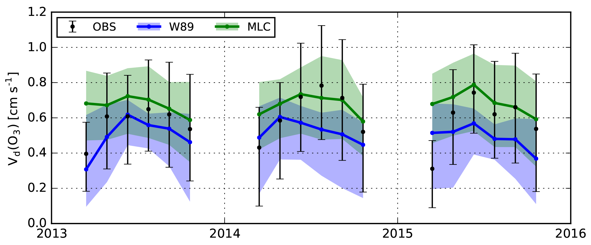
Figure 2Time series of April–September monthly average daytime (08:00–20:00 LT) ozone dry deposition velocity for Ispra, for W89 (blue), MLC-CHEM (green), and observations (black). Solid lines and points show monthly daytime medians for simulations and observations, respectively, and shaded areas and whiskers display the interquartile range.
3.1 Temporal variability in ozone dry deposition velocity
3.1.1 Monthly and interannual variability
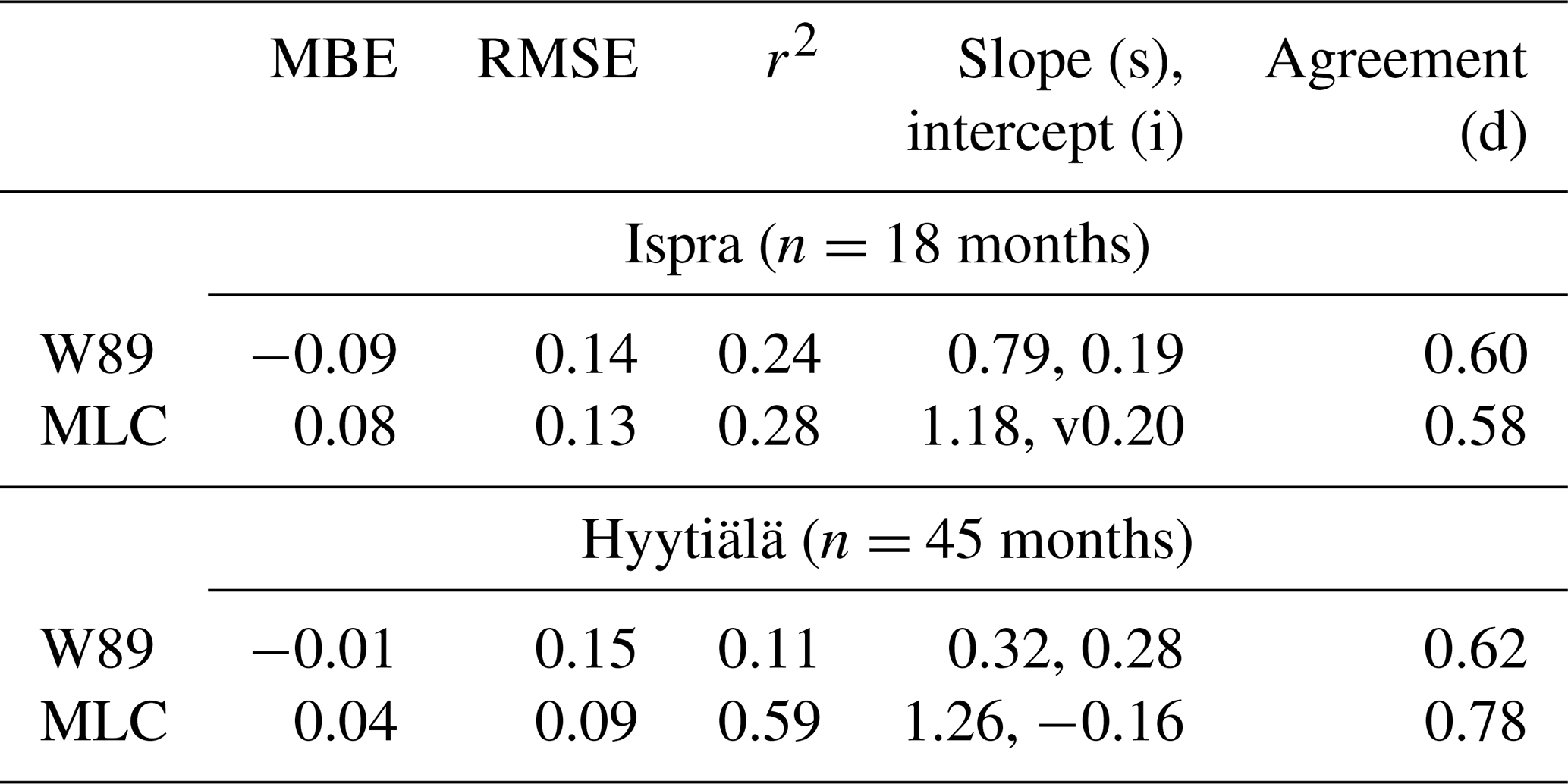
The observed ozone uptake at Ispra is generally highest in June–August, with little interannual variability (Fig. 2. W89 underestimates the observed dry deposition velocity (Vd(O3)) by ±0.1 cm s−1, while MLC-CHEM reproduces the observed magnitude of Vd(O3) within 7 % in May–September. On the basis of the statistical model performance metrics in Table 1, there is no parameterization that consistently outperforms the other on monthly timescales. MLC-CHEM systematically overestimates ozone deposition in April. To evaluate this bias further, we performed MLC-CHEM simulations with a deactivated sink to wet leaves, motivated by the considerable uncertainty in this ozone removal pathway (Clifton et al., 2020a). This simulation resulted in the strongest decrease in Vd(O3) in the relatively humid months of April (Fig. S2), ranging from 0.15 cm s−1 in April 2013 to 0.05 cm s−1 in April 2015. This modification results in an improved representation of seasonality in Vd(O3), suggesting seasonal variation in the ozone sink to wet leaves that might not be properly captured by the RH-dependent parameterization of wet leaf uptake (Eq. 4).
The observed Vd(O3) at Hyytiälä is generally lower compared to Ispra, reflecting a lower leaf area and, thus, less stomatal uptake at the Finnish site. W89 and MLC-CHEM both capture the observed magnitude of Vd(O3) to within the interquartile range of observations (±0.2 cm s−1) in most years, although Vd(O3) in W89 peaks 1 month early compared to the observations. MLC-CHEM reproduces the seasonal cycle in Vd(O3) with a Pearson (temporal) correlation coefficient between simulations and observations, which is markedly higher compared to the W89 approach (r2=0.59 for MLC-CHEM; r2=0.11 for W89; Table 1). These results suggest that MLC-CHEM better reproduces stomatal and non-stomatal removal processes, and we will investigate this further below.
The interannual variability in the ozone dry deposition velocity for Hyytiälä is 0.17 cm s−1 and is slightly underestimated in both simulations (0.10–0.11 cm s−1; not shown). We therefore calculated the contributions from stomatal conductance and non-stomatal conductance to the overall deposition velocity, as described in Sect. 2.2. Interannual variability in stomatal conductance is overestimated slightly by W89 and MLC-CHEM, compared to the observation-derived gs estimates, by 0.02 and 0.05 cm s−1, respectively. Interannual variability in non-stomatal conductance is strongly underestimated in both simulations (0.04–0.07 cm s−1) compared to the observed interannual variability in non-stomatal conductance (0.19 cm s−1). The missing interannual variability in the non-stomatal deposition pathway may be due the chemical, wet leaf, and soil uptake pathways.

Table 1Performance statistics for the monthly averaged simulations of Vd(O3) with W89 and MLC-CHEM (MLC). The unit is centimeters per second (cm s−1)for mean bias error (MBE), root mean square error (RMSE), and the intercept and unitless for the other metrics. Shown are several conventionally applied performance metrics (MBE, RMSE, slope (s) and intercept (i) of a linear regression fit of simulations against observations and r2 from the ordinary least squares regression) and the index of agreement (d).
3.1.2 Diurnal cycles
The observed diurnal cycle of Vd(O3) at Ispra (Fig. 4a) is characterized by an asymmetrical pattern, with a steep morning increase that plateaus around 0.8 cm s−1 and a decrease in the afternoon that reflects stomatal closure and reduced non-stomatal uptake. W89 underestimates the observed median daytime Vd(O3) values by ±0.1 cm s−1 (20 %), while MLC-CHEM reproduces the observations within 10 %. The onset of the W89-simulated daytime Vd(O3) peak shows a 1 h time lag, with an underestimation of around −0.3 cm s−1 (52 %) in the morning (06:00–10:00 LT) and an overestimation of 0.1 cm s−1 (13 %) in the afternoon (12:00–16:00 LT). The contribution of the stomatal and non-stomatal removal in this model–observation mismatch will be discussed in Sect.3.2. MLC-CHEM reproduces the diurnal course of Vd(O3) within 0.1 cm s−1 throughout the day.
The observed Vd(O3) diurnal cycle at Hyytiälä (Fig. 4b) increases earlier during the day, compared to Ispra, and decreases later, due to the extended day length during the growing season at the Finnish site. Vd(O3) peaks at 0.5 cm s−1 between 09:00–12:00 LT and decreases in the early afternoon due to decreasing (non-)stomatal sink ozone removal. W89 overestimates the magnitude of Vd(O3) by 0.1 cm s−1 (22 %) in the afternoon (12:00–16:00 LT) and underestimates ozone uptake in the morning (03:00–10:00 LT) and evening (after 19:00 LT). Apart from a morning overestimation by up to 0.1 cm s−1, MLC-CHEM reproduces the diurnal evolution of Vd(O3) well, which is apparently due to a more realistic representation of stomatal and non-stomatal removal processes.
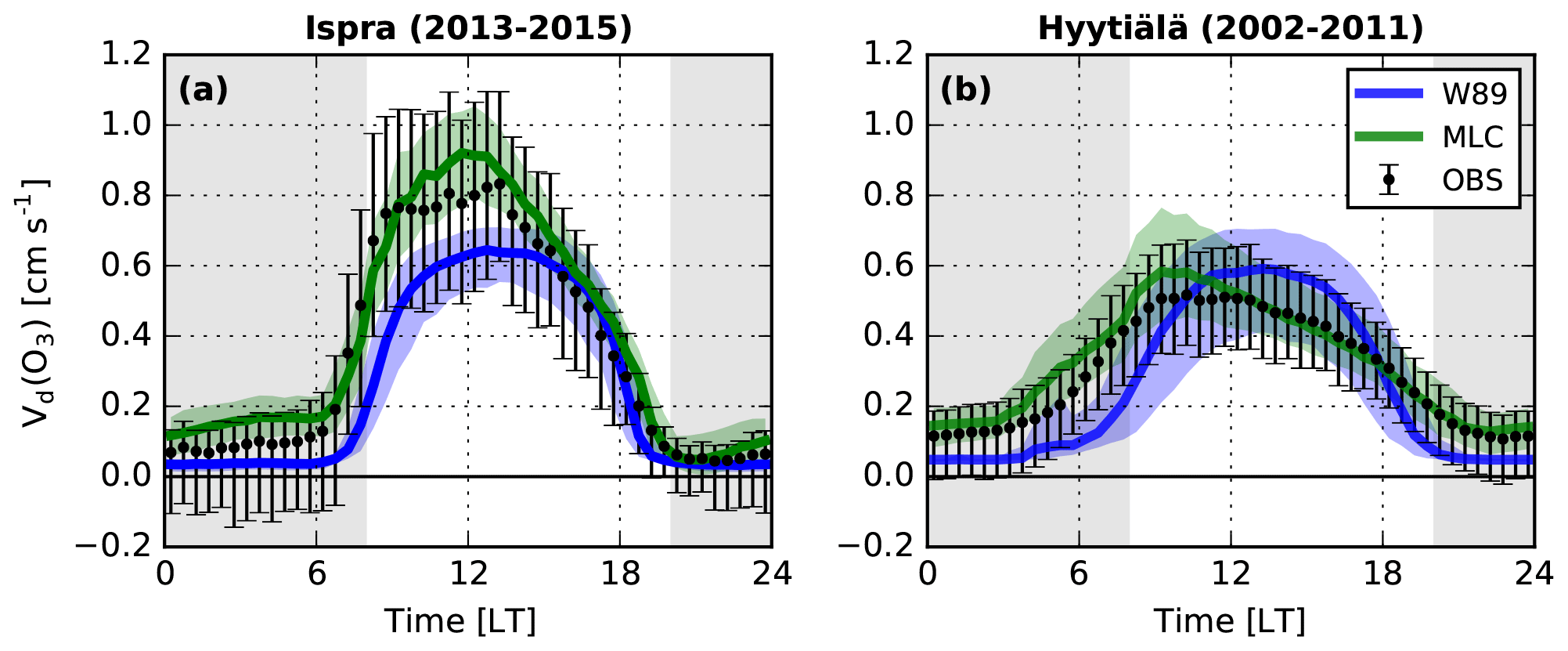
Figure 4Diurnal cycles of April–September ozone dry deposition velocity at Ispra (a) and Hyytiälä (b) derived from observations (black) and simulations with the W89 parameterization (blue) and MLC-CHEM (green). Lines and points show median values, and shaded areas and whiskers display the interquartile range.
3.2 Diurnal variability in stomatal and non-stomatal uptake
3.2.1 Ispra
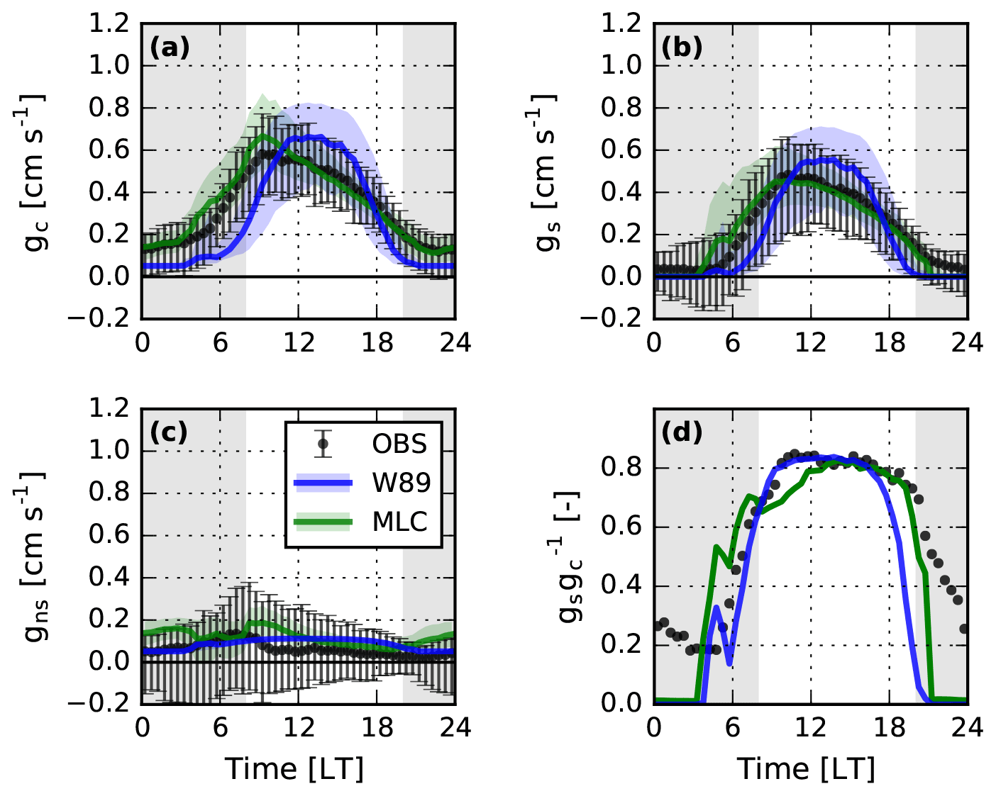
Next, we analyze the stomatal and non-stomatal components of ozone deposition to further understand the model–observation agreement on diurnal timescales. Figure 5 shows growing season median diurnal cycles of bulk canopy conductance (gc), canopy stomatal conductance (gs), and non-stomatal conductance (gns) for Ispra in W89 and MLC-CHEM simulation and observational estimates. At Ispra, the observation-derived daytime median ozone canopy conductance is 0.87 cm s−1 (Fig. 5a). The inferred daytime median stomatal conductance is as small as 0.26 cm s−1 (gray points in Fig. 5b), corresponding to a daytime stomatal uptake fraction of 35 % (Fig. 5d). However, we found a substantial gap (of 56 %) in the energy balance closure (Qgap), defined as the difference between net incoming radiation (Rn) and the surface energy balance components (Foken, 2008). This indicates underestimations in observed sensible and latent energy fluxes (H and LE), which affects our observation-derived stomatal conductance. The energy balance closure issues remain after filtering the observations based on quality flags and u* thresholds (Fig. S1).
To resolve these energy balance closure issues, we applied a correction method that partitions Qgap to H and LE via the evaporative fraction (EF = ; Twine et al., 2000; Renner et al., 2019). This correction increases LE and H by 156 and 25 W m−2, respectively, corresponding to an evaporative fraction of 0.86. With these corrected surface energy balance components, we derive a substantially larger daytime median stomatal conductance to ozone of 0.49 cm s−1 (black points in Fig. 5b, d), which is an increase of nearly 90 % with respect to the original observation-derived estimate. The Qgap correction also leads to a better model–observation agreement for gs. Ozone fluxes are also affected by the surface energy balance closure gap; additional data filtering based on u* thresholds leads to increases in observed ozone fluxes, which exceeds 50 % in the morning and evening when absolute fluxes are low, but the effect is smaller (< 15 %) during midday.
The observed diurnal cycle in canopy conductance at Ispra is better captured by MLC-CHEM compared to W89 (Fig. 5a). MLC-CHEM also better captures decreases in gc observed in the afternoon. MLC-CHEM and W89 simulate a daytime median ozone stomatal conductance of 0.43 and 0.51 cm s−1, respectively, and, thus, agree better with the Qgap-corrected stomatal conductance estimate derived from observations (Fig. 5b). The observation-derived stomatal fraction during 08:00–20:00 LT (0.62) is overestimated by W89 (0.72) and underestimated by MLC-CHEM (0.52). The observed stomatal uptake fraction increases throughout the day, from ±0.4 at 08:00 LT to ±0.8 at 18:00 LT, and this diurnal course is better reproduced by MLC-CHEM than by W89.
Observation-derived non-stomatal conductance peaks in the morning, levels off at ±0.8 cm s−1 (Fig. 5c; gray points), and decreases in the afternoon before reaching a nighttime value of 0.1 cm s−1. The stomatal conductance increase following Qgap correction leads to a reduction in the daytime average inferred non-stomatal conductance from 0.57 to 0.35 cm s−1. This correction does, however, not affect the shape of the diurnal cycle in gns, which is characterized by a sharp increase in the morning and a more gradual reduction in the afternoon. Daytime non-stomatal conductance is strongly underestimated by W89 and shows little diurnal variability since most in-canopy resistances are constant and, apparently, too high. MLC-CHEM reproduces the observed diurnal evolution in non-stomatal conductance more accurately than W89 (Fig. 5c), apparently due to its representation of diurnal variability in processes involved in non-stomatal removal, wet leaf uptake, and in-canopy turbulence. The contributions of different removal processes to total non-stomatal uptake will be discussed in Sect. 3.3.
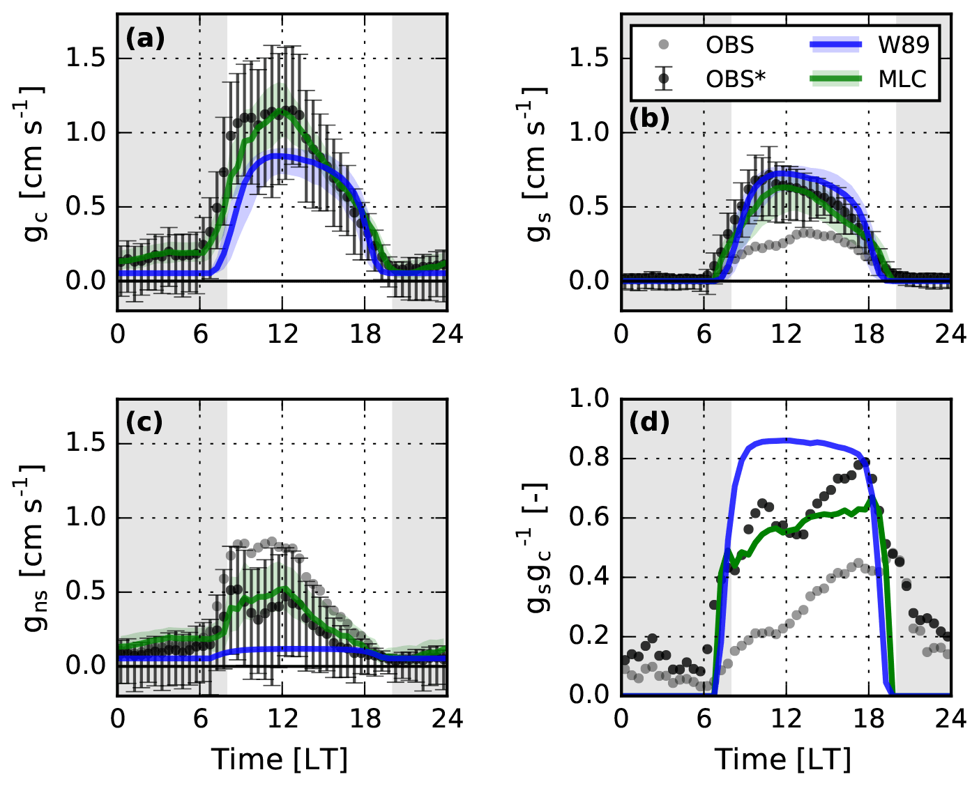
Figure 5April–September median diurnal cycles of ozone bulk canopy conductance (a), canopy stomatal conductance (b), bulk non-stomatal conductance, and (c) the stomatal fraction of total ozone removal (; d) for Ispra. Observed medians and interquartile ranges after Qgap correction (OBS*; see text) are shown as black points and whiskers (the values prior to Qgap correction, denoted as OBS, are shown in gray). The median and interquartile range of W89 and MLC-CHEM are shown in blue and green, respectively. The shaded area in panel (d) highlights the nighttime period (defined as 08:00–20:00 LT) during which the stomatal flux is calculated.
3.2.2 Hyytiälä
At Hyytiälä, the observation-derived daytime median gc is 0.53 cm s−1 (Fig. 6a), which is lower compared to Ispra due to lower non-stomatal ozone removal. W89 overestimates canopy conductance by up to 0.2 cm s−1 in the afternoon, while morning and evening gc are underestimated. Similar to Ispra, MLC-CHEM captures the diurnal evolution in gc better than W89, with a peak around 09:00 LT, as in the observations, but overestimates morning canopy conductance by 0.1 cm s−1. We did not correct for surface energy balance closure gaps for the Hyytiälä observations, since this gap was considerably smaller (±20 % of rn, without a distinct diurnal cycle) and in closer agreement to the literature-reported values for tall vegetation (Foken, 2008).
Observed stomatal conductance peaks at ±0.5 cm s−1 at 10:00 LT, followed by a decrease in the afternoon (Fig. 6b). W89 underestimates gs in the morning (05:00–10:00 LT), and overestimates afternoon values by 20 %–25 %. MLC-CHEM overestimates morning stomatal conductance, but follows the observed diurnal cycle well throughout the rest of the day. The observed stomatal ozone uptake fraction is relatively constant at 0.8 (Fig. 6), comparable to the upper range of stomatal uptake fraction estimates by Rannik et al. (2012). The stomatal fraction is well reproduced by both parameterizations, although for W89 this seems a coincidence given the misrepresented diurnal cycle in gc and gs.
Observation-derived non-stomatal conductance at Hyytiälä (Fig. 6c) is relatively constant at 0.1 cm s−1, except for a morning peak of 0.2 cm s−1 around 08:00 LT that likely reflects wet leaf ozone uptake (Altimir et al., 2006; Rannik et al., 2012). W89 reproduces the observed daytime magnitude of gns but cannot reproduce its morning peak. MLC-CHEM overestimates the nighttime non-stomatal ozone sink, in line with a study by Zhou et al. (2017) based on a 1-month time series of ozone flux observations (August 2010), indicating that observed nighttime ozone deposition appears to reflect smaller nocturnal soil uptake efficiency than assumed. Except for an overestimation in the morning, MLC-CHEM captures the observation-inferred magnitude of non-stomatal ozone deposition well during daytime.
3.3 Dependence of non-stomatal deposition on driving variables
Non-stomatal ozone uptake, and its dependence on micro-meteorological and other environmental drivers, is incompletely understood. Previous studies employed statistical or process-oriented modeling (Rannik et al., 2012; Fares et al., 2014; El-Madany et al., 2017; Clifton et al., 2019) to determine the contribution of driving variables to this ozone sink. In this section, we study observed and simulated relationships between the non-stomatal ozone removal fraction () and two variables (air temperature, Ta, and VPD) that we hypothesize to contribute to temporal variability in non-stomatal ozone removal. This section focuses on non-stomatal ozone removal at Ispra, since Rannik et al. (2012) previously characterized the non-stomatal ozone sink for Hyytiälä, and we compare our findings for Ispra to their results at the end of this section.
We first determine how W89 and MLC-CHEM can reproduce the observed relationship between non-stomatal ozone removal and Ta and VPD. We focus on the average daytime response (08:00–20:00 LT) and, subsequently, on three different periods in the diurnal cycle (06:00–20:00, 10:00–14:00, and 14:00–18:00 LT). In this manner, we can disentangle processes affecting (non-)stomatal uptake that act during different periods of the diurnal cycle (wet leaf uptake in the morning, optimal stomatal functioning during midday, and suppressed stomatal conductance during the afternoon).
The temperature response of the relative contribution of non-stomatal removal to total ozone deposition (expressed by the non-stomatal fraction, ) during different periods of the diurnal cycle is shown in Fig. 7a–d. Non-stomatal uptake decreases with temperature during the day (Fig. 7a). This decrease is largely driven by the morning temperature sensitivity of , which shows less sensitivity to temperature later during the day (Fig. 7b–d). W89 underestimates the observed temperature dependence of the non-stomatal fraction throughout the day by ±0.2, although the morning non-stomatal fraction is higher for the lowest temperature bin (10–15 ∘C). MLC-CHEM reproduces the daytime response well, as it is characterized by elevated morning non-stomatal uptake under low-temperature conditions. For most temperature bins, W89 strongly underestimates the observed variability in the non-stomatal fraction. The observed variability is also underestimated by MLC-CHEM, although to a smaller extent, and apparently indicates still missing or misrepresented deposition processes.
The observation-derived non-stomatal fraction increases with VPD during daytime (Fig. 7e–h), indicating that non-stomatal ozone removal decreases under dry conditions. This result contradicts an anticipated increase in the contribution by non-stomatal removal to overall canopy removal due to a VPD-induced decrease in stomatal uptake. However, the observed non-stomatal uptake also decreases in the afternoon (Fig. 5c) and, therefore, does not compensate for the decreasing stomatal sink with VPD. The non-stomatal fraction displays the strongest VPD sensitivity in the morning, which mainly reflects simulated wet leaf uptake under humid (i.e., low VPD) conditions. Non-stomatal removal in W89 is insensitive to VPD, and this parameterization particularly underestimates the non-stomatal fraction under humid conditions (Fig. 7a–b). MLC-CHEM reproduces the daytime slope between VPD and the non-stomatal fraction well.
We then perform a number of sensitivity experiments with MLC-CHEM with deactivated non-stomatal sinks to identify the role of each sink in explaining temporal variability in non-stomatal ozone removal and its dependence on Ta and VPD. In these experiments, we exclude the contribution by wet leaf uptake, soil uptake, and in-canopy chemical removal, as well as an experiment with strongly enhanced turbulent exchange between the crown layer and the understory. In the Supplement, Sect. S2 and Fig. S6 display the results from the sensitivity analysis of non-stomatal removal at Ispra. We list the main outcomes of this section and the MLC-CHEM sensitivity analysis as follows:
-
Soil deposition accounts for almost 40 % of non-stomatal removal under high-temperature conditions, reflecting a simulated increase in in-canopy turbulent transport with air temperature.
-
Non-stomatal uptake is elevated under cold and humid conditions in the morning. This is consistent with MLC-CHEM-simulated wet leaf uptake, which accounts for over 20 % of the morning non-stomatal removal fraction.
-
Enhanced turbulent transport from the crown layer to the understory reduces the non-stomatal uptake fraction in MLC-CHEM, as it leads to enhanced stomatal uptake in the understory.
-
Chemical removal plays a minor role in the total canopy ozone sink at Ispra.
In their multivariate analysis of environmental drivers of non-stomatal ozone removal at Hyytiälä, Rannik et al. (2012) derived that air temperature and VPD are significantly associated with variations in non-stomatal ozone removal, similar to our findings for Ispra. However, Rannik et al. (2012) also found an explanatory role for monoterpene concentrations at Hyytiälä, while our results suggest a minor role of chemical removal at Ispra.
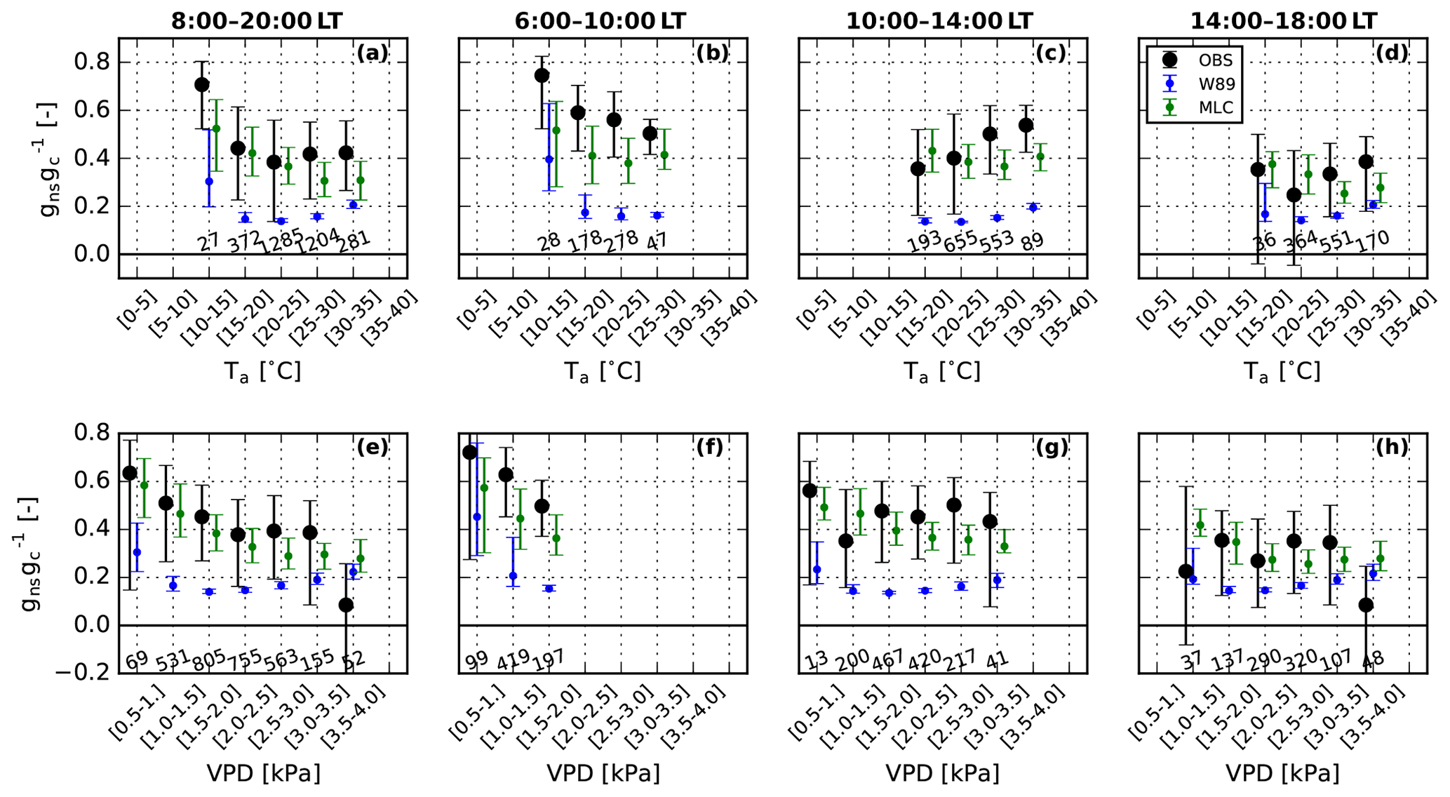
Figure 7Non-stomatal ozone removal fraction binned by air temperature (a–d) and vapor pressure deficit (e–h) during June–September 2013–2015 at Ispra. Black dots and whiskers show from observations and simulations by W89 (blue points and whiskers) and MLC-CHEM (green points and whiskers). Dots and whiskers display the median and interquartile range per bin, respectively, and the number of observations in the bin is displayed at the bottom of the panels. Each column corresponds to a different time period in the diurnal cycle, namely all day (08:00–20:00 LT; a, e), morning (06:00–10:00 LT; b, f), midday (10:00–14:00 LT; c, g), and afternoon (14:00–18:00 LT; d, h). Dots and whiskers are only shown if the number of samples in the bin exceeds 10.
3.4 Cumulative uptake of ozone (CUO)
In the previous sections, we have shown that the seasonal evolution of ozone deposition in W89 and MLC-CHEM is relatively similar. However, there are consistent differences in daytime ozone stomatal and non-stomatal sinks between the deposition representations. In this section, we evaluate the implications of these differences in the representation of (non-)stomatal removal for determining the cumulative stomatal uptake of ozone (CUO) over the growing season, which is often used for ozone impact assessments (Musselman et al., 2006; Mills et al., 2011). We here use the term CUOst to refer to cumulative stomatal uptake and to distinguish this from cumulative non-stomatal ozone removal (CUOns). In Fig. 8, we compare growing-season-integrated stomatal and non-stomatal ozone fluxes from W89 and MLC-CHEM to observation-derived estimates of total seasonal ozone uptake for both sites (Fig. 8a, c). Our observation-based derivation of stomatal conductance requires dry conditions (RH < 90 %, and no precipitation in the preceding 12 h) to avoid overestimations in the observation-inferred stomatal conductance which lead to overestimations in CUO. However, the application of these data selection criteria also leads to a reduction in data points that hinders the calculation of CUOst based on observations. In order to derive a first-order CUOst estimate, we divide the cumulative stomatal uptake inferred from valid observations by the fraction of valid observations. This method serves mainly to perform a site-to-site comparison of inferred CUOst. Inferred CUOst at Ispra varies between 61 and 72 mmol m−2 (Fig. 8b). The inferred CUOst in 2014 was lower compared to 2013 and 2015 due to comparatively low ozone mixing ratios, while stomatal conductance displayed less year-to-year variability. At Hyytiälä, inferred CUOst varies between 39 and 41 mmol m−2 (Fig. 8d), where the lower value in 2005 (29 mmol m−2) is caused by missing data during June–August, when stomatal ozone uptake peaks. The higher inferred CUOst values at Ispra compared to Hyytiälä reflect both higher stomatal conductance and ozone mixing ratios at the Italian site.
The differences between W89- and MLC-CHEM-simulated conductances are also manifested in the simulated growing season cumulative (stomatal) uptake (Fig. 8a–c). The cumulative total ozone flux for Ispra is underestimated by W89 (−10 %), while this parameterization overestimates cumulative stomatal uptake by 14 %–22 %. MLC-CHEM accurately reproduces observation-derived CUOst (within 7 %) but overestimates the cumulative total flux by 15 % (Fig. 8a). Therefore, the model–observation agreement of the two parameterizations for the simulated cumulative total ozone removal largely reflects non-stomatal uptake differences, which deviates from observation-inferred values by −64 % and 51 %, respectively. At Hyytiälä, the observed cumulative total ozone flux is 15.1 mmol m−2 and is overestimated by 34 % by W89, reflecting overestimated stomatal uptake (Fig. 8c). The observation-derived CUOst is 12.6 mmol m−2, compared to 15.8 mmol m−2 in W89 (+28 %) and 12.3 mmol m−2 in MLC-CHEM (−2.4 %). We conclude that the better representation of canopy stomatal conductance in MLC-CHEM compared to W89, particularly during the afternoon peak in ozone mixing ratios, may lead to a substantially reduced bias in the simulated growing-season-integrated (stomatal) ozone flux.

Figure 8(a, c) Growing-season-integrated daytime (08:00–20:00 LT) and stomatal (CUOst; dark colors) and non-stomatal (CUOns; light colors) ozone fluxes for the different years in the study period for Ispra (a) and Hyytiälä (c). Results from the W89 parameterization are shown in blue, MLC-CHEM in green, and observations in gray. Only the data points with valid observation-inferred stomatal conductance estimates are selected for this comparison; the fraction of valid data points per growing season that remains is shown at the bottom of panels (a, c). (b, d) Inferred cumulative stomatal ozone uptake (CUO) estimate at both sites (hatched bars) after dividing the season-integrated daytime stomatal ozone flux (dark gray bars) by the fraction of valid data points. Note the different y axis ranges across the four panels.
This study evaluates the potential added value of a multi-layer representation of vegetation canopies with respect to a commonly applied big leaf approach (W89; Wesely, 1989) for simulating ozone deposition and ozone impact metrics for forest canopies. We focus on short- to long-term temporal variability in Vd(O3) and its partitioning into stomatal and non-stomatal components, as well as the simulation of ozone impact metrics. We find that both parameterizations reasonably reproduce the observed seasonal cycle in Vd(O3), which is in agreement with previous chemistry transport model evaluations (e.g., Hardacre et al., 2015). Despite their comparable performance on seasonal timescales, the parameterizations deviate in their simulation of the diurnal cycle; the W89 parameterization particularly underestimates morning ozone removal by 52 % (Ispra) and 37 % (Hyytiälä), due to a combination of underestimated stomatal removal and a missing non-stomatal sink, which is likely wet leaf uptake. In the afternoon, W89 deviates less from observations at both sites (−13 % at Ispra; +22 % at Hyytiälä). Consequently, cumulative stomatal ozone uptake is overestimated by, on average, 18 % (Ispra) and 28 % (Hyytiälä) in W89 simulations, while cumulative total ozone removal deviates by −10 % (Ispra) and 20 % (Hyytiälä). Ozone mixing ratios typically peak in the afternoon and, thus, occur simultaneously with stomatal conductance misrepresentations, which may lead to simulated ozone fluxes overestimates using this mechanism. The multi-layer mechanism, constrained with latent energy and net ecosystem exchange (NEE) observations to optimally represent stomatal exchange, displays a better agreement with the observed ozone deposition velocity (within 10 %) and inferred cumulative stomatal and total uptake (within 15 % and 9 % for Ispra and Hyytiälä, respectively). Therefore, an accurate representation of diurnal variability in ozone uptake partitioned to stomatal and non-stomatal sinks is essential for reproducing cumulative (stomatal) ozone uptake at the land surface.
We applied a big leaf parameterization that is commonly used in (regional) atmospheric chemistry models, for example in WRF-Chem (Grell et al., 2005; Galmarini et al., 2021). Big leaf parameterizations advantageously depend on a limited number of routinely available meteorological variables and a simplified description of land use characteristics and can be readily applied at any location without location-specific parameter derivations (Clifton et al., 2020a). However, the empirical nature of these schemes leads to an oversimplification of in-canopy physical and chemical processes that affect atmosphere–biosphere exchange of ozone, e.g., by not accounting for stomatal closure based on the vapor pressure deficit (VPD) and soil moisture or in-canopy chemical reactions. There are big leaf versions available with a more process-based description of ozone deposition processes, particularly for stomatal conductance (e.g., Lin et al., 2019; Clifton et al., 2020c; Emberson et al., 2001; Büker et al., 2012) and non-stomatal ozone removal (Zhang et al., 2003).
To further explore the effect of model assumptions in big leaf parameterizations, we performed a comparison between W89 and another commonly used big leaf dry deposition scheme by Zhang et al. (2003, referred to as Z03) in Appendix B. This parameterization includes a separate treatment of sunlit versus shaded leaves and the explicit treatment of water stress in the stomatal conductance calculation and includes variations in non-stomatal resistances as a function of LAI and u*. We find that both parameterizations overestimate afternoon stomatal conductance compared to observations, while Z03 better reproduces morning gs (Fig. B1). The differences between these parameterizations are, therefore, largely driven by differences in non-stomatal ozone removal (Fig. B1). The agreement with observation-inferred non-stomatal removal depends on site-specific conditions, particularly friction velocity. Our analyses highlight potential areas of improvement in process representation that can be considered in future larger-scale modeling studies to improve the simulations of ozone deposition pathways and their temporal variability. This is particularly important for season-integrated (stomatal) ozone fluxes with big leaf parameterizations.
Our results suggest that Anet-gs parameterizations, as applied in MLC-CHEM, simulate stomatal conductance in good agreement with observation-inferred values throughout the diurnal cycle. Such models are sensitive to parameters typically derived at leaf level that display spatiotemporal variability. Further observational constraints on these parameters, e.g., from leaf-level ecophysiological measurements, improve the representation of stomatal conductance and biosphere–atmosphere exchange (Vilà-Guerau De Arellano et al., 2020), benefitting simulations of CO2 and ozone exchange as simulated by Anet-gs within MLC-CHEM. Determining these parameters from canopy-top observations is an underdetermined problem in a mathematical sense, which we circumvented by deriving a realistic set of model parameters based on a comparison with canopy-top observed NEE and observation-derived stomatal conductance, while remaining as close as possible to the original parameter set in Ronda et al. (2001). Choosing Anet-gs parameters could be formalized by applying mathematical techniques such as data assimilation (Raoult et al., 2016).
MLC-CHEM can be driven by diagnostic variables available from the chemical transport model (CTM) output (or their driving meteorological models), favoring its implementation to represent atmosphere–biosphere fluxes of reactive compounds (Ganzeveld et al., 2002, 2010). In such a coupled setup, MLC-CHEM would use simulated stomatal conductance from the driving model to represent an atmosphere–biosphere exchange consistent with the model's representation of (micro-)meteorology. An implementation of A-gs with CO2 mixing ratios, calculated online or offline, can be tested if simulated stomatal conductance estimates are unavailable.
Our analysis did not include soil moisture as a predictor of stomatal conductance. Sensitivity simulations in MLC-CHEM with observation-constrained soil water content (SWC) at different depths resulted in strong reductions in simulated NEE and gs during summer compared to observations, which suggests that these SWC observations are not indicative of root zone soil moisture. Nonetheless, simulations of ozone deposition and mixing ratios at various spatial scales suggest a higher predictive skill when accounting for SWC (Anav et al., 2018; Lin et al., 2019, 2020; Clifton et al., 2020c; Otu-Larbi et al., 2020). Including this stress term is especially important in the context of projected drought risk and intensity increases in future climate scenarios (Cook et al., 2018) that may aggravate ozone smog episodes due to a decreased stomatal sink (Lin et al., 2020).
Our analysis of non-stomatal ozone removal as a function of micro-meteorological drivers (air temperature and VPD) for Ispra reveals that the non-stomatal sink is elevated under low-VPD (i.e., high-RH) morning conditions, likely indicating uptake at the leaf surface in water films formed by dew (Zhang et al., 2002; Potier et al., 2015). This sink is reproduced by MLC-CHEM by applying a wet canopy fraction dependent on RH and a constant wet skin uptake resistance. Observations suggest that this non-stomatal ozone sink is less important at Hyytiälä, which could be due to a lower RH threshold for the development of wet canopy conditions in MLC-CHEM compared to previous work (Altimir et al., 2006; Zhou et al., 2017). Since wet leaf uptake may affect simulated diurnal cycles of ozone in chemistry transport models (Travis and Jacob, 2019), uptake parameterizations would benefit from better observation-based constraints on this removal process, both in terms of canopy wetness and wet leaf uptake efficiency.
Our sensitivity analysis also reveals an important role of soil deposition during the afternoon due to more active in-canopy transport. We applied a constant soil resistance to ozone uptake in our simulations, despite various environmental controls that have been identified, including air temperature, soil water content, near-surface air humidity, and soil clay content (Fares et al., 2014; Fumagalli et al., 2016; Stella et al., 2011, 2019). Our results suggest a minor importance of chemical ozone removal at the two considered sites. However, we did not investigate the role of ozone scavenging by reactive sesquiterpenes (Zhou et al., 2017; Hellén et al., 2018; Vermeuel et al., 2021) or soil-emitted nitric oxide (Finco et al., 2018). Since most (big leaf) parameterizations work with a poorly constrained resistance to transport from the canopy-top to the soil (e.g., Makar et al., 2017), the importance of the chemical and soil ozone sinks for total canopy ozone removal can be best explored with better resolved in-canopy turbulent exchange in model simulations.
We have shown that stomatal and non-stomatal sinks are not accurately reproduced using the W89 big leaf parameterization compared to observations at two forested ozone flux sites, leading to structurally biased instantaneous and growing season cumulated (stomatal) ozone flux simulations. Improved methods (e.g., the DO3SE mechanism, Emberson et al., 2001; Büker et al., 2012) do correct for soil moisture and VPD in the stomatal conductance calculation. Overestimated stomatal ozone fluxes also likely have implications for simulated ozone mixing ratios. Many models underestimate midday ozone mixing ratios in Europe (Solazzo et al., 2012; Im et al., 2015; Visser et al., 2019), and a misrepresentation of land surface uptake may contribute to this bias. Therefore, an overestimated ozone deposition flux may also affect the simulation of concentration-based vegetation ozone impact metrics, such as AOT40, in the opposite direction compared to flux-based metrics. An improved model representation of the ozone deposition process will provide more confidence in the application of atmospheric chemistry models for surface air quality and vegetation ozone damage assessments.
To stimulate improvement of big leaf and multi-layer parameterizations, modelers may benefit from evaluations against existing long-term dry deposition observations in various ecosystems (e.g., forests and grassland) and for contrasting environmental conditions (e.g., during dry vs. wet seasons). Such an assessment is currently underway in stage 4 of the Air Quality Model Evaluation International Initiative (AQMEII4; Galmarini et al., 2021). Additionally, evaluation against in- and above-canopy ozone flux measurements (Fares et al., 2014; Finco et al., 2018) can reveal information about non-stomatal sinks in these parameterizations, such as soil deposition and in-canopy chemical removal. Last, the application of proposed parameterizations for non-stomatal ozone sinks, such as for wet leaf uptake (Potier et al., 2015) and soil uptake (Stella et al., 2019), should be tested in 3D and in single-point models of ozone deposition.
We compare ozone deposition simulations to multi-year observations at two European forested flux sites, with a focus on temporal variability, contributions from stomatal and non-stomatal sinks, and metrics for the damage incurred by ozone on vegetation. The widely used big leaf parameterization Wesely (W89; 1989) and the in-canopy process-resolving MLC-CHEM model both reproduce the seasonal cycle of daytime ozone deposition velocity reasonably well, but there are important differences in the skill of the two approaches to capture the diurnal changes in ozone deposition. Specifically, W89 consistently underestimates ozone deposition velocities in the morning (by 37 %–52 %), while the afternoon model observation is somewhat smaller (−13 %–22 %). MLC-CHEM captures the diurnal cycle much better, with relatively small biases, in the morning (−9 % at Ispra, +17 % at Hyytiälä) and has good agreement (within 10 %) in the afternoon. Accounting for stomatal closure, wet leaf removal and in-canopy turbulent transport followed by soil uptake turns out to be important for accurately simulating ozone deposition on diurnal timescales.
The structural errors in W89 are explained by a misrepresentation of the diurnal cycle in stomatal and non-stomatal conductance. Simulations with a more recent big leaf parameterization result in similar biases regarding stomatal and non-stomatal uptake. The MLC-CHEM model, constrained by local observations of diurnal CO2 and latent energy fluxes, captures stomatal and non-stomatal ozone conductance better. As a result, W89 systematically overestimates cumulative ozone uptake by 20 %–30 % in the growing season at Ispra and Hyytiälä, whereas MLC-CHEM reproduces cumulative ozone uptake within 3 % at both sites. We conclude that MLC-CHEM, nudged with observation-inferred stomatal conductance, accurately describes non-stomatal uptake processes and vegetation ozone impact metrics.
Sensitivity tests with MLC-CHEM for Ispra point out that, in relatively cold and humid conditions, ozone deposition on wet leaves appears to explain up to 20 % of the non-stomatal ozone sink. During high-temperature conditions characterized by efficient in-canopy transport, enhanced uptake by soils accounts for up to 40 % of non-stomatal ozone deposition. The tests suggest a minor role for chemical destruction of ozone at Ispra.
Our results indicate that current model representations of stomatal and non-stomatal ozone uptake by vegetation, often based on W89, should be thoroughly evaluated. This study provides a strategy for such evaluations and shows how a more detailed, canopy-resolving model driven by ancillary measurements of CO2 and energy fluxes can provide more realistic estimates of ozone deposition and vegetation ozone impact metrics.
Prior to applying MLC-CHEM to analyze ozone fluxes at our study sites, we first paid attention to simulations of the canopy CO2 flux () and canopy stomatal conductance (gs) to ensure that the photosynthesis parameterization (A-gs) functions satisfactorily. An initial simulation with the default settings for the C3 vegetation class resulted in a strongly overestimated compared to observations at both sites (see Table A2). This is accompanied by strong overestimation of the canopy stomatal conductance at Ispra, while MLC-CHEM slightly underestimates stomatal conductance at Hyytiälä.
The default A-gs settings were derived for low vegetation such as grassland and crops (Ronda et al., 2001) and are therefore not necessarily representative for forest canopies. We performed a sensitivity analysis of simulated and gs to A-gs model parameters in order to determine optimized parameter sets for our simulations. These settings are given in Table A1. We found that strongly overestimated is largely caused by a presumed high reference mesophyll conductance (gm,298), leading to overestimated transport of CO2 in the plant's chloroplast. Our reductions in gm,298 are in better correspondence with previously reported estimates of 0.8–2.0 mm s−1 for different forest plant functional types (Steeneveld, 2002; Voogt et al., 2006; ECMWF, 2020). At Ispra, we additionally modified the mesophyll conductance temperature response curve, which differs between plant species (Calvet et al., 1998; von Caemmerer and Evans, 2015), to improve the amplitude of the seasonal cycle in simulated . At Hyytiälä, the maximum internal CO2 concentration (f0, given as a fraction of the external CO2 concentration) was increased to improve the correspondence with observation-derived gs.
Our observational constraints to A-gs lead to improved simulations of gs and (Table A2). The parameter changes additionally affect the simulation of the ozone dry deposition velocity (Vd(O3)), as shown in Table A3. At Ispra, the strong reduction in stomatal conductance leads to an underestimation in Vd(O3) (MBE = −0.12 cm s−1), while the other statistical metrics indicate a modest model improvement. At Hyytiälä, the growing season model overestimation is slightly reduced from 0.04 to 0.02 cm s−1. Our approach results in a reduced model bias at the two study sites, particularly for , while taking care to stay as close as possible to the original parameter set.
Table A1A-gs parameter settings used in MLC-CHEM simulations. The first column indicates the default C3 settings from Ronda et al. (2001), and the other two columns show the optimal settings from our analysis. A dash (–) indicates that a parameter is unchanged with respect to the default C3 value.
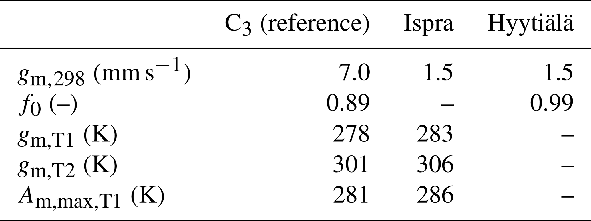
Table A2Model performance statistics of MLC-CHEM before and after A-gs optimization for canopy stomatal conductance and CO2 flux. Shown are several conventionally applied performance metrics (MBE, RMSE, slope (s), and intercept (i) of a linear regression fit of simulations against observations and r2 from ordinary least squares regression), as well as the index of agreement (d). The units are centimeters per second (cm s−1) and micromoles per square meter per second (µmol m−2 s−1), respectively, unless indicated otherwise.
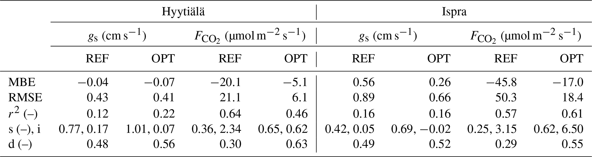
Table A3As in Table A2 but for Vd(O3) (in centimeters per second; cm s−1).
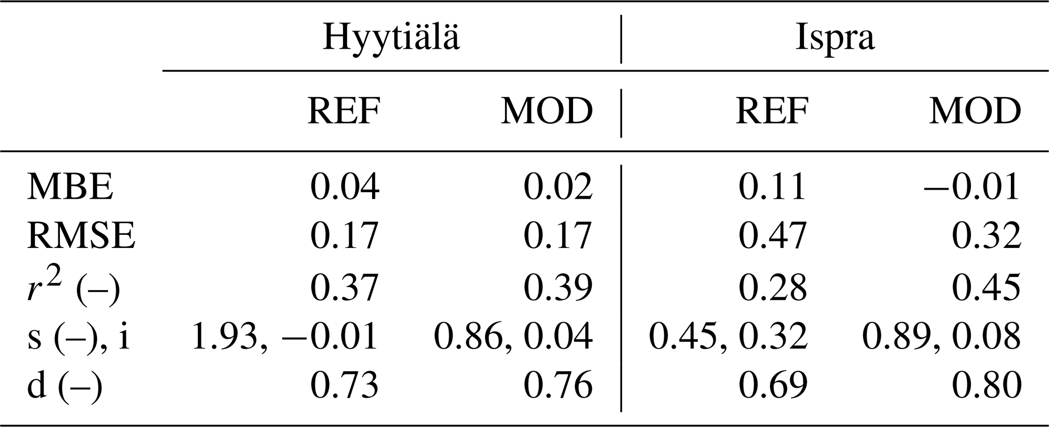
In order to derive more generic conclusions about big leaf parameterizations, we considered another commonly applied parameterization (Zhang et al., 2003) that has recently been extended to different gases by Wu et al. (2018). This big leaf formulation (hereafter Z03) differs compared to the Wesely (1989) parameterization (hereafter W89) in several aspects, as follows: (1) Z03 calculates stomatal conductance for sunlit and shaded leaves differently, (2) stomatal conductance is affected by VPD and soil moisture stress, and (3) non-stomatal resistances contain seasonal and diurnal variability due to dependencies on leaf area index and friction velocity (u*). This model version was derived from Zhang and Wu (2021) with two modifications. First, we adapted the soil resistance to locally derived values of 400 s m−1 (Hyytiälä) and 300 s m−1 (Ispra), similar to W89 and MLC-CHEM (see Sect. 2). The implementation by Zhang and Wu (2021) relies on observed canopy wetness, which is not available for our two study sites. We therefore parameterize canopy wetness as a function of relative humidity, analogous to MLC-CHEM (Eq. 4). In this section, we compare simulations by W89 and Z03 to observations of the ozone dry deposition velocity and observation-inferred stomatal and non-stomatal conductance.
Figure B1 shows multi-year growing season median diurnal cycles of Vd(O3), gs and gns for Ispra and Hyytiälä. From this analysis, we conclude that W89 and Z03 perform similarly for Ispra compared against observed Vd(O3) (Fig. B1a). Z03 better captures the early morning onset of Vd(O3) for Hyytiälä than W89, but more strongly overestimates midday and afternoon Vd(O3) compared to observations (Fig. B1b). Both parameterizations overestimate midday and afternoon gs, while Z03 better captures the observed morning and afternoon gs values than W89 (Fig. B1c, d). For gns, there is no parameterization that performs best for the two sites. Both parameterizations underestimate observation-inferred gns at Ispra (corrected for energy balance closure gaps; see Sect. 3.2), while W89 better captures the magnitude of observation-inferred gns (although Z03 better reproduces the shape of the diurnal cycle). This suggests that the gns dependence on u* is less strong in the observations than is suggested in the Z03 parameterization; i.e., a sensitivity experiment with doubled u* values for Ispra results in daytime gns values of 0.2–0.35 cm s−1, which is an increase by a factor 2.3–2.8. Based on our findings, we conclude that the different representation of non-stomatal ozone removal drives the differences between W89 and Z03, but the magnitude of these differences depends on site-specific conditions.
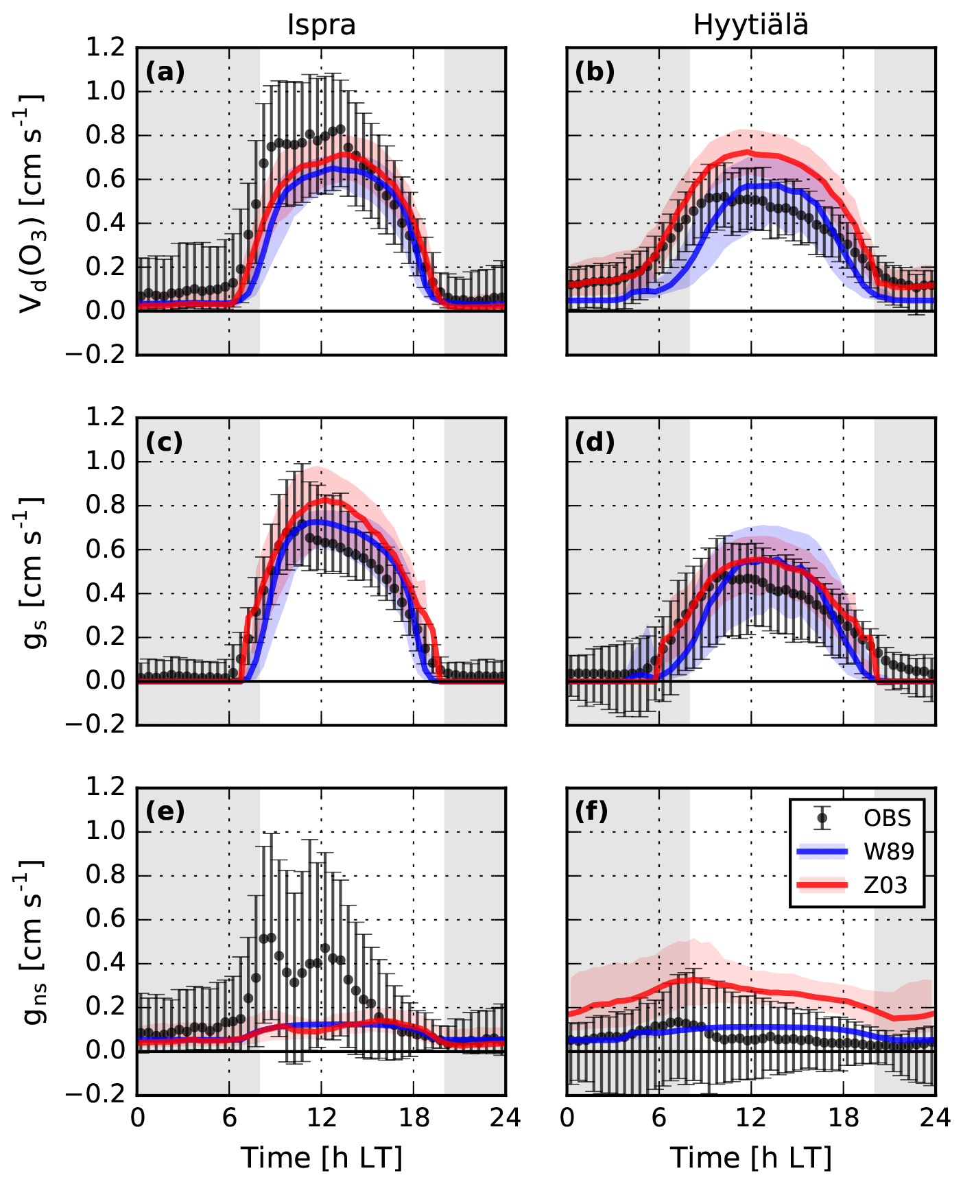
Figure B1Comparison of the dry deposition parameterizations W89 (Wesely, 1989) and Z03 (Zhang et al., 2003) against the observed dry deposition velocity (a, b) and observation-inferred stomatal conductance (c, d) and non-stomatal conductance (e, f) for Ispra and Hyytiälä (left and right panels, respectively). Lines and shaded areas (points and whiskers) show April–September median and interquartile range of the simulations (observations).
MLC-CHEM source code and model output are available upon request to the corresponding author.
The supplement related to this article is available online at: https://doi.org/10.5194/acp-21-18393-2021-supplement.
AJV, LNG, and KFB designed the experiments, and AJV performed the simulations and data analysis. IG, IM, and GM provided observational data and expertise on the use thereof in this study. AJV wrote the paper, with contributions from all co-authors.
At least one of the (co-)authors is a member of the editorial board of Atmospheric Chemistry and Physics. The peer-review process was guided by an independent editor, and the authors also have no other competing interests to declare.
Publisher’s note: Copernicus Publications remains neutral with regard to jurisdictional claims in published maps and institutional affiliations.
The authors acknowledge the public availability of observational data sets used in this study via the European Fluxes Database Cluster (http://gaia.agraria.unitus.it, last access: 12 July 2021) and the Finnish research data portal (https://etsin.fairdata.fi, last access: 12 July 2021).
This research has been supported by the Nederlandse Organisatie voor Wetenschappelijk Onderzoek (grant no. ALW-GO 16/17). The observational infrastructure at Hyytiälä is funded under the ACCC flagship by the Academy of Finland (grant no. 337549).
This paper was edited by Leiming Zhang and reviewed by two anonymous referees.
Ainsworth, E. E. A., Yendrek, C. R., Sitch, S., Collins, W. J., and Emberson, L. D.: The effects of tropospheric ozone on net primary productivity and implications for climate change., Annu. Rev. Plant Biol., 63, 637–61, https://doi.org/10.1146/annurev-arplant-042110-103829, 2012. a
Altimir, N., Kolari, P., Tuovinen, J.-P., Vesala, T., Bäck, J., Suni, T., Kulmala, M., and Hari, P.: Foliage surface ozone deposition: a role for surface moisture?, Biogeosciences, 3, 209–228, https://doi.org/10.5194/bg-3-209-2006, 2006. a, b, c
Anav, A., Proietti, C., Menut, L., Carnicelli, S., De Marco, A., and Paoletti, E.: Sensitivity of stomatal conductance to soil moisture: implications for tropospheric ozone, Atmos. Chem. Phys., 18, 5747–5763, https://doi.org/10.5194/acp-18-5747-2018, 2018. a
Arnold, S. R., Lombardozzi, D., Lamarque, J. F., Richardson, T., Emmons, L. K., Tilmes, S., Sitch, S. A., Folberth, G., Hollaway, M. J., and Val Martin, M.: Simulated Global Climate Response to Tropospheric Ozone-Induced Changes in Plant Transpiration, Geophys. Res. Lett., 45, 13070–13079, https://doi.org/10.1029/2018GL079938, 2018. a, b
Bates, K. H. and Jacob, D. J.: An Expanded Definition of the Odd Oxygen Family for Tropospheric Ozone Budgets: Implications for Ozone Lifetime and Stratospheric Influence, Geophys. Res. Lett., 47, 1–9, https://doi.org/10.1029/2019GL084486, 2020. a
Büker, P., Morrissey, T., Briolat, A., Falk, R., Simpson, D., Tuovinen, J.-P., Alonso, R., Barth, S., Baumgarten, M., Grulke, N., Karlsson, P. E., King, J., Lagergren, F., Matyssek, R., Nunn, A., Ogaya, R., Peñuelas, J., Rhea, L., Schaub, M., Uddling, J., Werner, W., and Emberson, L. D.: DO3SE modelling of soil moisture to determine ozone flux to forest trees, Atmos. Chem. Phys., 12, 5537–5562, https://doi.org/10.5194/acp-12-5537-2012, 2012. a, b
Calvet, J. C., Noilhan, J., Roujean, J. L., Bessemoulin, P., Cabelguenne, M., Olioso, A., and Wigneron, J. P.: An interactive vegetation SVAT model tested against data from six contrasting sites, Agr. Forest Meteorol., 92, 73–95, https://doi.org/10.1016/S0168-1923(98)00091-4, 1998. a
Clifton, O. E., Fiore, A. M., Munger, J. W., Malyshev, S., Horowitz, L. W., Shevliakova, E., Paulot, F., Murray, L. T., and Griffin, K. L.: Interannual variability in ozone removal by a temperate deciduous forest, Geophysical Research Letters, 44, 542–552, https://doi.org/10.1002/2016GL070923, 2017. a, b, c, d
Clifton, O. E., Fiore, A. M., Munger, J. W., and Wehr, R.: Spatiotemporal Controls on Observed Daytime Ozone Deposition Velocity Over Northeastern U.S. Forests During Summer, J. Geophys. Res.-Atmos., 124, 5612–5628, https://doi.org/10.1029/2018JD029073, 2019. a, b, c
Clifton, O. E., Fiore, A. M., Massman, W. J., Baublitz, C. B., Coyle, M., Emberson, L., Fares, S., Farmer, D. K., Gentine, P., Gerosa, G., Guenther, A. B., Helmig, D., Lombardozzi, D. L., Munger, J. W., Patton, E. G., Pusede, S. E., Schwede, D. B., Silva, S. J., Sörgel, M., Steiner, A. L., and Tai, A. P.: Dry Deposition of Ozone over Land: Processes, Measurement, and Modeling, Rev. Geophys., 58, e2019RG000670, https://doi.org/10.1029/2019rg000670, 2020a. a, b, c, d, e, f
Clifton, O. E., Lombardozzi, D. L., Fiore, A. M., Paulot, F., and Horowitz, L. W.: Stomatal conductance influences interannual variability and long-term changes in regional cumulative plant uptake of ozone, Environ. Res. Lett., 15, 114059, https://doi.org/10.1088/1748-9326/abc3f1, 2020b. a
Clifton, O. E., Paulot, F., Fiore, A. M., Horowitz, L. W., Correa, G., Baublitz, C. B., Fares, S., Goded, I., Goldstein, A. H., Gruening, C., Hogg, A. J., Loubet, B., Mammarella, I., Munger, J. W., Neil, L., Stella, P., Uddling, J., Vesala, T., and Weng, E.: Influence of Dynamic Ozone Dry Deposition on Ozone Pollution, J. Geophys. Res.-Atmos., 125, 1–21, https://doi.org/10.1029/2020JD032398, 2020c. a, b, c
Cook, B. I., Mankin, J. S., and Anchukaitis, K. J.: Climate Change and Drought: From Past to Future, Curr. Clim., 4, 164–179, https://doi.org/10.1007/s40641-018-0093-2, 2018. a
Ducker, J. A., Holmes, C. D., Keenan, T. F., Fares, S., Goldstein, A. H., Mammarella, I., Munger, J. W., and Schnell, J.: Synthetic ozone deposition and stomatal uptake at flux tower sites, Biogeosciences, 15, 5395–5413, https://doi.org/10.5194/bg-15-5395-2018, 2018. a
ECMWF: Part IV: Physical Processes, in: IFS Documentation CY47R1, June, p. 228, ECMWF, Reading, United Kingdom, available at: https://www.ecmwf.int/node/19748 (last acces: 13 December 2021), 2020. a
El-Madany, T. S., Niklasch, K., and Klemm, O.: Stomatal and non-stomatal turbulent deposition flux of ozone to a managed peatland, Atmosphere, 8, 1–16, https://doi.org/10.3390/atmos8090175, 2017. a, b
Emberson, L. D., Wieser, G., and Ashmore, M. R.: Modelling of stomatal conductance and ozone flux of Norway spruce: comparison with field data, Environ. Pollut., 109, 393–402, 2000. a
Emberson, L. D., Ashmore, M., Simpson, D., Tuovinen, J.-P., and Cambridge, H.: Modelling and mapping ozone deposition in Europe, Water Air Soil Pollut., 130, 577–582, https://doi.org/10.1023/A:1013851116524, 2001. a, b
Erisman, J. W., Van Pul, A., and Wyers, P.: Parametrization of surface resistance for the quantification of atmospheric deposition of acidifying pollutants and ozone, Atmos. Environ., 28, 2595–2607, https://doi.org/10.1016/1352-2310(94)90433-2, 1994. a
Fares, S., Savi, F., Muller, J., Matteucci, G., and Paoletti, E.: Simultaneous measurements of above and below canopy ozone fluxes help partitioning ozone deposition between its various sinks in a Mediterranean Oak Forest, Agr. Forest Meteorol., 198, 181–191, https://doi.org/10.1016/j.agrformet.2014.08.014, 2014. a, b, c, d, e
Finco, A., Coyle, M., Nemitz, E., Marzuoli, R., Chiesa, M., Loubet, B., Fares, S., Diaz-Pines, E., Gasche, R., and Gerosa, G.: Characterization of ozone deposition to a mixed oak–hornbeam forest – flux measurements at five levels above and inside the canopy and their interactions with nitric oxide, Atmos. Chem. Phys., 18, 17945–17961, https://doi.org/10.5194/acp-18-17945-2018, 2018. a, b, c
Foken, T.: The energy balance closure problem: An overview, Ecol. Appl., 18, 1351–1367, https://doi.org/10.1890/06-0922.1, 2008. a, b
Fowler, D., Flechard, C., Neil Cape, J., Storeton-West, R., and Coyle, M.: Measurements of ozone deposition to vegetation quantifying the flux, the stomatal and non-stomatal components, Water Air Soil Pollut., 130, 63–74, https://doi.org/10.1023/A:1012243317471, 2001. a
Fowler, D., Pilegaard, K., Sutton, M. A., Ambus, P., Raivonen, M., Duyzer, J., Simpson, D., Fagerli, H., Fuzzi, S., Schjoerring, J. K., Granier, C., Neftel, A., Isaksen, I. S. A., Laj, P., Maione, M., Monks, P. S., Burkhardt, J., Daemmgen, U., Neirynck, J., Personne, E., Wichink-Kruit, R., Butterbach-Bahl, K., Flechard, C., Tuovinen, J. P., Coyle, M., Gerosa, G., Loubet, B., Altimir, N., Gruenhage, L., Ammann, C., Cieslik, S., Paoletti, E., Mikkelsen, T. N., Ro-Poulsen, H., Cellier, P., Cape, J. N., Horváth, L., Loreto, F., Niinemets, Ü., Palmer, P. I., Rinne, J., Misztal, P., Nemitz, E., Nilsson, D., Pryor, S., Gallagher, M. W., Vesala, T., Skiba, U., Brüggemann, N., Zechmeister-Boltenstern, S., Williams, J., O'Dowd, C., Facchini, M. C., de Leeuw, G., Flossman, A., Chaumerliac, N., and Erisman, J. W.: Atmospheric composition change: Ecosystems-Atmosphere interactions, Atmos. Environ., 43, 5193–5267, https://doi.org/10.1016/j.atmosenv.2009.07.068, 2009. a, b
Fumagalli, I., Gruening, C., Marzuoli, R., Cieslik, S., and Gerosa, G.: Long-term measurements of NOx and O3 soil fluxes in a temperate deciduous forest, Agr. Forest Meteorol., 228-229, 205–216, https://doi.org/10.1016/j.agrformet.2016.07.011, 2016. a, b, c, d, e
Galmarini, S., Makar, P., Clifton, O. E., Hogrefe, C., Bash, J. O., Bellasio, R., Bianconi, R., Bieser, J., Butler, T., Ducker, J., Flemming, J., Hodzic, A., Holmes, C. D., Kioutsioukis, I., Kranenburg, R., Lupascu, A., Perez-Camanyo, J. L., Pleim, J., Ryu, Y.-H., San Jose, R., Schwede, D., Silva, S., and Wolke, R.: Technical note: AQMEII4 Activity 1: evaluation of wet and dry deposition schemes as an integral part of regional-scale air quality models, Atmos. Chem. Phys., 21, 15663–15697, https://doi.org/10.5194/acp-21-15663-2021, 2021. a, b, c
Ganzeveld, L. and Lelieveld, J.: Dry deposition parameterization in a chemistry general circulation model and its influence on the distribution of reactive trace gases, J. Geophys. Res., 100, 95JD02266, https://doi.org/10.1029/95jd02266, 1995. a, b
Ganzeveld, L., Lelieveld, J., and Roelofs, G. J.: A dry deposition parameterization for sulfur oxides in a chemistry and general circulation model, J. Geophys. Res.-Atmos., 103, 5679–5694, https://doi.org/10.1029/97JD03077, 1998. a
Ganzeveld, L., Bouwman, L., Stehfest, E., van Vuuren, D., Eickhout, B., and Lelieveld, J.: Impacts of future land cover changes on atmospheric chemistry-climate interactions, J. Geophys. Res., 115, 2010JD014041, https://doi.org/10.1029/2010JD014041, 2010. a, b, c, d
Ganzeveld, L. N., Lelieveld, J., Dentener, F. J., Krol, M. C., and Roelofs, G. J.: Atmosphere-biosphere trace gas exchanges simulated with a single-column model, J. Geophys. Res.-Atmos., 107, 1–21, https://doi.org/10.1029/2001JD000684, 2002. a, b, c, d, e, f
Grell, G. A., Peckham, S. E., Schmitz, R., Mckeen, S. A., Frost, G., Skamarock, W. C., and Eder, B.: Fully coupled “online” chemistry within the WRF model, Atmos. Environ., 39, 6957–6975, https://doi.org/10.1016/j.atmosenv.2005.04.027, 2005. a, b
Gruening, C., Goded, I., Cescatti, A., Fachinetti, D., Fumagalli, I., and Duerr, M.: ABC-IS Forest Flux Station Report on Instrumentation , Operational Testing and First Months of Measurements, Tech. Rep., Joint Research Centre, Ispra, https://doi.org/10.2788/7774, 2012. a
Guenther, A., Karl, T., Harley, P., Wiedinmyer, C., Palmer, P. I., and Geron, C.: Estimates of global terrestrial isoprene emissions using MEGAN (Model of Emissions of Gases and Aerosols from Nature), Atmos. Chem. Phys., 6, 3181–3210, https://doi.org/10.5194/acp-6-3181-2006, 2006. a
Guenther, A. B., Jiang, X., Heald, C. L., Sakulyanontvittaya, T., Duhl, T., Emmons, L. K., and Wang, X.: The Model of Emissions of Gases and Aerosols from Nature version 2.1 (MEGAN2.1): an extended and updated framework for modeling biogenic emissions, Geosci. Model Dev., 5, 1471–1492, https://doi.org/10.5194/gmd-5-1471-2012, 2012. a
Hardacre, C., Wild, O., and Emberson, L.: An evaluation of ozone dry deposition in global scale chemistry climate models, Atmos. Chem. Phys., 15, 6419–6436, https://doi.org/10.5194/acp-15-6419-2015, 2015. a
Hellén, H., Praplan, A. P., Tykkä, T., Ylivinkka, I., Vakkari, V., Bäck, J., Petäjä, T., Kulmala, M., and Hakola, H.: Long-term measurements of volatile organic compounds highlight the importance of sesquiterpenes for the atmospheric chemistry of a boreal forest, Atmos. Chem. Phys., 18, 13839–13863, https://doi.org/10.5194/acp-18-13839-2018, 2018. a
Hicks, B. B., Baldocchi, D. D., Meyers, T. P., Hosker, R. P., and Matt, D. R.: A preliminary multiple resistance routine for deriving dry deposition velocities from measured quantities, Water Air Soil Pollut., 36, 311–330, https://doi.org/10.1007/BF00229675, 1987. a
Hu, L., Jacob, D. J., Liu, X., Zhang, Y., Zhang, L., Kim, P. S., Sulprizio, M. P., and Yantosca, R. M.: Global budget of tropospheric ozone: Evaluating recent model advances with satellite (OMI), aircraft (IAGOS), and ozonesonde observations, Atmos. Environ., 167, 323–334, https://doi.org/10.1016/j.atmosenv.2017.08.036, 2017. a
Im, U., Bianconi, R., Kioutsioukis, I., Badia, A., Bellasio, R., Brunner, D., Balzarini, A., Bar, R., Chemel, C., Curci, G., Flemming, J., Forkel, R., Giordano, L., Hirtl, M., Hodzic, A., Honzak, L., Jorba, O., Jim, P., Knote, C., Kuenen, J. J. P., Makar, P. A., Manders-groot, A., Pirovano, G., Pouliot, G., San, R., Neal, L., Juan, L. P., Savage, N., Schroder, W., Sokhi, R. S., Syrakov, D., Torian, A., Tuccella, P., Werhahn, J., Wolke, R., Yahya, K., Zabkar, R., Zhang, Y., Zhang, J., and Hogrefe, C.: Evaluation of operational on-line-coupled regional air quality models over Europe and North America in the context of AQMEII phase 2, Part I: Ozone, Atmos. Environ., 115, 404–420, https://doi.org/10.1016/j.atmosenv.2014.09.042, 2015. a
Knauer, J., El-Madany, T. S., Zaehle, S., and Migliavacca, M.: Bigleaf—An R package for the calculation of physical and physiological ecosystem properties from eddy covariance data, PLoS ONE, 13, 1–26, https://doi.org/10.1371/journal.pone.0201114, 2018. a
Lammel, G.: Formation of nitrous acid: parameterisation and comparison with observations, Tech. Rep. 286, Max-Planck-Institut für Meteorologie, Hamburg, DE, available at: https://pure.mpg.de/pubman/faces/ViewItemOverviewPage.jsp?itemId=item_3187907 (last acces: 13 December 2021), 1999. a
Launiainen, S., Katul, G. G., Grönholm, T., and Vesala, T.: Partitioning ozone fluxes between canopy and forest floor by measurements and a multi-layer model, Agr. Forest Meteorol., 173, 85–99, https://doi.org/10.1016/j.agrformet.2012.12.009, 2013. a
Lin, M., Malyshev, S., Shevliakova, E., Paulot, F., Horowitz, L. W., Fares, S., Mikkelsen, T. N., and Zhang, L.: Sensitivity of Ozone Dry Deposition to Ecosystem-Atmosphere Interactions: A Critical Appraisal of Observations and Simulations, Global Biogeochem. Cy., 33, 1264–1288, https://doi.org/10.1029/2018GB006157, 2019. a, b, c, d
Lin, M., Horowitz, L. W., Xie, Y., Paulot, F., Malyshev, S., Shevliakova, E., Finco, A., Gerosa, G., Kubistin, D., and Pilegaard, K.: Vegetation feedbacks during drought exacerbate ozone air pollution extremes in Europe, Nat. Clim. Change, 10, 444–451, https://doi.org/10.1038/s41558-020-0743-y, 2020. a, b
Lombardozzi, D., Levis, S., Bonan, G., Hess, P. G., and Sparks, J. P.: The influence of chronic ozone exposure on global carbon and water cycles, J. Climate, 28, 292–305, https://doi.org/10.1175/JCLI-D-14-00223.1, 2015. a, b
Makar, P. A., Staebler, R. M., Akingunola, A., Zhang, J., McLinden, C., Kharol, S. K., Pabla, B., Cheung, P., and Zheng, Q.: The effects of forest canopy shading and turbulence on boundary layer ozone, Nat. Commun., 8, 1–14, https://doi.org/10.1038/ncomms15243, 2017. a, b
Mammarella, I., Peltola, O., Nordbo, A., Järvi, L., and Rannik, Ü.: Quantifying the uncertainty of eddy covariance fluxes due to the use of different software packages and combinations of processing steps in two contrasting ecosystems, Atmos. Meas. Tech., 9, 4915–4933, https://doi.org/10.5194/amt-9-4915-2016, 2016. a
Mills, G., Pleijel, H., Braun, S., Büker, P., Bermejo, V., Calvo, E., Danielsson, H., Emberson, L., Fernández, I. G., Grünhage, L., Harmens, H., Hayes, F., Karlsson, P. E., and Simpson, D.: New stomatal flux-based critical levels for ozone effects on vegetation, Atmos. Environ., 45, 5064–5068, https://doi.org/10.1016/j.atmosenv.2011.06.009, 2011. a
Monteith, J.: Evaporation and Environment, Symposia of the Society for Experimental Biology, 19, 205–234, available at: https://repository.rothamsted.ac.uk/item/8v5v7 (last acces: 13 December 2021), 1965. a
Musselman, R. C., Lefohn, A. S., Massman, W. J., and Heath, R. L.: A critical review and analysis of the use of exposure- and flux-based ozone indices for predicting vegetation effects, Atmos. Environ., 40, 1869–1888, https://doi.org/10.1016/j.atmosenv.2005.10.064, 2006. a
Otu-Larbi, F., Conte, A., Fares, S., Wild, O., and Ashworth, K.: Current and future impacts of drought and ozone stress on Northern Hemisphere forests, Global Change Biol., 26, 6218–6234, https://doi.org/10.1111/gcb.15339, 2020. a, b
Potier, E., Ogée, J., Jouanguy, J., Lamaud, E., Stella, P., Personne, E., Durand, B., Mascher, N., and Loubet, B.: Multilayer modelling of ozone fluxes on winter wheat reveals large deposition on wet senescing leaves, Agr. Forest Meteorol., 211, 58–71, https://doi.org/10.1016/j.agrformet.2015.05.006, 2015. a, b, c
Rannik, Ü., Altimir, N., Mammarella, I., Bäck, J., Rinne, J., Ruuskanen, T. M., Hari, P., Vesala, T., and Kulmala, M.: Ozone deposition into a boreal forest over a decade of observations: evaluating deposition partitioning and driving variables, Atmos. Chem. Phys., 12, 12165–12182, https://doi.org/10.5194/acp-12-12165-2012, 2012. a, b, c, d, e, f, g, h
Raoult, N. M., Jupp, T. E., Cox, P. M., and Luke, C. M.: Land-surface parameter optimisation using data assimilation techniques: the adJULES system V1.0, Geosci. Model Dev., 9, 2833–2852, https://doi.org/10.5194/gmd-9-2833-2016, 2016. a
Renner, M., Brenner, C., Mallick, K., Wizemann, H.-D., Conte, L., Trebs, I., Wei, J., Wulfmeyer, V., Schulz, K., and Kleidon, A.: Using phase lags to evaluate model biases in simulating the diurnal cycle of evapotranspiration: a case study in Luxembourg, Hydrol. Earth Syst. Sci., 23, 515–535, https://doi.org/10.5194/hess-23-515-2019, 2019. a
Ronda, R., De Bruin, H., and Holtslag, A.: Representation of the canopy conductance in modeling the surface energy budget for low vegetation, J. Appl. Meteorol., 40, 1431–1444, https://doi.org/10.1175/1520-0450(2001)040<1431:ROTCCI>2.0.CO;2, 2001. a, b, c, d, e, f
Sadiq, M., Tai, A. P. K., Lombardozzi, D., and Val Martin, M.: Effects of ozone–vegetation coupling on surface ozone air quality via biogeochemical and meteorological feedbacks, Atmos. Chem. Phys., 17, 3055–3066, https://doi.org/10.5194/acp-17-3055-2017, 2017. a, b
Sitch, S., Cox, P. M., Collins, W. J., and Huntingford, C.: Indirect radiative forcing of climate change through ozone effects on the land-carbon sink, Nature, 448, 791–794, https://doi.org/10.1038/nature06059, 2007. a
Solazzo, E., Bianconi, R., Vautard, R., Appel, K. W., Moran, M., Hogrefe, C., Bessagnet, B., Brandt, J., Christensen, J. H., Chemel, C., Coll, I., Denier van der Gon, H., Ferreira, J., Forkel, R., Francis, X. V., Grell, G., Grossi, P., Hansen, A. B., Jeričević, A., Kraljević, L., Miranda, A. I., Nopmongcol, U., Pirovano, G., Prank, M., Riccio, A., Sartelet, K. N., Schaap, M., Silver, J. D., Sokhi, R. S., Vira, J., Werhahn, J., Wolke, R., Yarwood, G., Zhang, J., Rao, T. S., and Galmarini, S.: Model evaluation and ensemble modelling of surface-level ozone in Europe and North America in the context of AQMEII, Atmos. Environ., 53, 60–74, https://doi.org/10.1016/j.atmosenv.2012.01.003, 2012. a
Steeneveld, G.: On photosynthesis parameters for the A-gs surface scheme for high vegetation, 1–79, available at: https://cdn.knmi.nl/knmi/pdf/bibliotheek/knmipubTR/TR242.pdf, (last access: 13 December 2021), 2002. a
Stella, P., Loubet, B., Lamaud, E., Laville, P., and Cellier, P.: Ozone deposition onto bare soil: A new parameterisation, Agr. Forest Meteorol., 151, 669–681, https://doi.org/10.1016/j.agrformet.2011.01.015, 2011. a, b
Stella, P., Loubet, B., de Berranger, C., Charrier, X., Ceschia, E., Gerosa, G., Finco, A., Lamaud, E., Serça, D., George, C., and Ciuraru, R.: Soil ozone deposition: Dependence of soil resistance to soil texture, Atmos. Environ., 199, 202–209, https://doi.org/10.1016/j.atmosenv.2018.11.036, 2019. a, b, c
Tai, A. P. K., Martin, M. V., and Heald, C. L.: Threat to future global food security from climate change and ozone air pollution, Nat. Clim. Change, 4, 817–821, https://doi.org/10.1038/nclimate2317, 2014. a
Travis, K. R. and Jacob, D. J.: Systematic bias in evaluating chemical transport models with maximum daily 8 h average (MDA8) surface ozone for air quality applications: a case study with GEOS-Chem v9.02, Geosci. Model Dev., 12, 3641–3648, https://doi.org/10.5194/gmd-12-3641-2019, 2019. a
Twine, T. E., Kustas, W. P., Norman, J. M., Cook, D. R., Houser, P. R., Meyers, T. P., Prueger, J. H., Starks, P. J., and Wesely, M. L.: Correcting eddy-covariance flux underestimates over a grassland, Agr. Forest Meteorol., 103, 279–300, https://doi.org/10.1016/S0168-1923(00)00123-4, 2000. a
Val Martin, M., Heald, C. L., and Arnold, S. R.: Coupling dry deposition to vegetation phenology in the Community Earth System Model: Implications for the simulation of surface O3, Geophys. Res. Lett., 41, 2988–2996, https://doi.org/10.1002/2014GL059651, 2014. a
Vermeuel, M. P., Cleary, P. A., Desai, A. R., and Bertram, T. H.: Simultaneous Measurements of O3 and HCOOH Vertical Fluxes Indicate Rapid In-Canopy Terpene Chemistry Enhances O3 Removal Over Mixed Temperate Forests, Geophys. Res. Lett., 48, 1–15, https://doi.org/10.1029/2020GL090996, 2021. a
Vilà-Guerau de Arellano, J., Ney, P., Hartogensis, O., de Boer, H., van Diepen, K., Emin, D., de Groot, G., Klosterhalfen, A., Langensiepen, M., Matveeva, M., Miranda-García, G., Moene, A. F., Rascher, U., Röckmann, T., Adnew, G., Brüggemann, N., Rothfuss, Y., and Graf, A.: CloudRoots: integration of advanced instrumental techniques and process modelling of sub-hourly and sub-kilometre land–atmosphere interactions, Biogeosciences, 17, 4375–4404, https://doi.org/10.5194/bg-17-4375-2020, 2020. a
Visser, A. J., Boersma, K. F., Ganzeveld, L. N., and Krol, M. C.: European NOx emissions in WRF-Chem derived from OMI: impacts on summertime surface ozone, Atmos. Chem. Phys., 19, 11821–11841, https://doi.org/10.5194/acp-19-11821-2019, 2019. a
von Caemmerer, S. and Evans, J. R.: Temperature responses of mesophyll conductance differ greatly between species, Plant Cell Environ., 38, 629–637, https://doi.org/10.1111/pce.12449, 2015. a
Voogt, M., Van den Hurk, B., and Jacobs, C.: The ECMWF land surface scheme extended with a photosynthesis and LAI module tested for a coniferous site, available at: https://cdn.knmi.nl/knmi/pdf/bibliotheek/knmipubWR/WR2006-02.pdf (last access: 13 December 2021), 2006. a
Wesely, M. L.: Parameterization of surface resistances to gaseous dry deposition in regional-scale numerical models, Atmos. Environ., 23, 1293–1304, https://doi.org/10.1016/j.atmosenv.2007.10.058, 1989. a, b, c, d, e, f, g, h, i, j, k
Wu, Z., Schwede, D. B., Vet, R., Walker, J. T., Shaw, M., Staebler, R., and Zhang, L.: Evaluation and Intercomparison of Five North American Dry Deposition Algorithms at a Mixed Forest Site, J. Adv. Model. Earth Sy., 10, 1571–1586, https://doi.org/10.1029/2017MS001231, 2018. a
Xiao, Z., Liang, S., Wang, J., Chen, P., Yin, X., Zhang, L., and Song, J.: Use of general regression neural networks for generating the GLASS leaf area index product from time-series MODIS surface reflectance, IEEE T. Geosci. Remote, 52, 209–223, https://doi.org/10.1109/TGRS.2013.2237780, 2014. a
Yáñez-Serrano, A. M., Nölscher, A. C., Bourtsoukidis, E., Gomes Alves, E., Ganzeveld, L., Bonn, B., Wolff, S., Sa, M., Yamasoe, M., Williams, J., Andreae, M. O., and Kesselmeier, J.: Monoterpene chemical speciation in a tropical rainforest:variation with season, height, and time of dayat the Amazon Tall Tower Observatory (ATTO), Atmos. Chem. Phys., 18, 3403–3418, https://doi.org/10.5194/acp-18-3403-2018, 2018. a
Yienger, J. and Levy, H.: Empirical model of global soil-biogenic NOx emissions, J. Geophys. Res., 100, 447–458, https://doi.org/10.1029/95JD00370, 1995. a
Zhang, L. and Wu, Z.: A computer code for calculating dry deposition velocities for 45 gaseous species, Zenodo [code], https://doi.org/10.5281/zenodo.4697426, 2021. a, b
Zhang, L., Brook, J. R., and Vet, R.: On ozone dry deposition – With emphasis on non-stomatal uptake and wet canopies, Atmos. Environ., 36, 4787–4799, https://doi.org/10.1016/S1352-2310(02)00567-8, 2002. a, b
Zhang, L., Brook, J. R., and Vet, R.: A revised parameterization for gaseous dry deposition in air-quality models, Atmos. Chem. Phys., 3, 2067–2082, https://doi.org/10.5194/acp-3-2067-2003, 2003. a, b, c, d, e, f
Zhou, P., Ganzeveld, L., Rannik, Ü., Zhou, L., Gierens, R., Taipale, D., Mammarella, I., and Boy, M.: Simulating ozone dry deposition at a boreal forest with a multi-layer canopy deposition model, Atmos. Chem. Phys., 17, 1361–1379, https://doi.org/10.5194/acp-17-1361-2017, 2017. a, b, c, d, e
- Abstract
- Introduction
- Data and methods
- Results
- Discussion
- Conclusions
- Appendix A: A-gs optimization
- Appendix B: Comparison between two big leaf parameterizations
- Code and data availability
- Author contributions
- Competing interests
- Disclaimer
- Acknowledgements
- Financial support
- Review statement
- References
- Supplement