the Creative Commons Attribution 4.0 License.
the Creative Commons Attribution 4.0 License.
 | 13 Dec 2021
Estimating 2010–2015 anthropogenic and natural methane emissions in Canada using ECCC surface and GOSAT satellite observations
Sabour Baray
Daniel J. Jacob
Joannes D. Maasakkers
Jian-Xiong Sheng
Melissa P. Sulprizio
Dylan B. A. Jones
A. Anthony Bloom
Robert McLaren
Methane emissions in Canada have both anthropogenic and natural sources. Anthropogenic emissions are estimated to be 4.1 Tg a−1 from 2010–2015 in the National Inventory Report submitted to the United Nation's Framework Convention on Climate Change (UNFCCC). Natural emissions, which are mostly due to boreal wetlands, are the largest methane source in Canada and highly uncertain, on the order of ∼ 20 Tg a−1 in biosphere process models. Aircraft studies over the last several years have provided “snapshot” emissions that conflict with inventory estimates. Here we use surface data from the Environment and Climate Change Canada (ECCC) in situ network and space-borne data from the Greenhouse Gases Observing Satellite (GOSAT) to determine 2010–2015 anthropogenic and natural methane emissions in Canada in a Bayesian inverse modelling framework. We use GEOS-Chem to simulate anthropogenic emissions comparable to the National Inventory and wetlands emissions using an ensemble of WetCHARTS v1.0 scenarios in addition to other minor natural sources. We conduct a comparative analysis of the monthly natural emissions and yearly anthropogenic emissions optimized by surface and satellite data independently. Mean 2010–2015 posterior emissions using ECCC surface data are 6.0 ± 0.4 Tg a−1 for total anthropogenic and 11.6 ± 1.2 Tg a−1 for total natural emissions. These results agree with our posterior emissions of 6.5 ± 0.7 Tg a−1 for total anthropogenic and 11.7 ± 1.2 Tg a−1 for total natural emissions using GOSAT data. The seasonal pattern of posterior natural emissions using either dataset shows slower to start emissions in the spring and a less intense peak in the summer compared to the mean of WetCHARTS scenarios. We combine ECCC and GOSAT data to characterize limitations towards sectoral and provincial-level inversions. We estimate energy + agriculture emissions to be 5.1 ± 1.0 Tg a−1, which is 59 % higher than the national inventory. We attribute 39 % higher anthropogenic emissions to Western Canada than the prior. Natural emissions are lower across Canada. Inversion results are verified against independent aircraft data and surface data, which show better agreement with posterior emissions. This study shows a readjustment of the Canadian methane budget is necessary to better match atmospheric observations with lower natural emissions partially offset by higher anthropogenic emissions.
- Article
(3960 KB) - Full-text XML
-
Supplement
(2514 KB) - BibTeX
- EndNote


Methane is a significant anthropogenically influenced greenhouse gas second to carbon dioxide in terms of its direct radiative forcing (Myhre, 2013). The mixing ratio of methane has increased from ∼ 720 to ∼ 1800 ppb since pre-industrial times (Hartmann et al., 2013). Present-day global methane emissions are well known to be 550 ± 60 Tg a−1 (Prather et al., 2012). However recent trends in atmospheric methane since the 1990s are not well understood (Turner et al., 2019). Anthropogenic methane sources include oil and gas activities, livestock, rice cultivation, coal mines, landfills and wastewater treatment. Natural methane emissions are dominated by wetlands but also include seeps, termites and biomass burning (Kirschke et al., 2013). The main sink of methane is oxidation by the hydroxyl radical (OH), resulting in a lifetime of 9.1 ± 0.9 years (Prather et al., 2012). Improving constraints on national methane emissions is a requirement of mitigation policy (Nisbet et al., 2020). Here we use atmospheric methane observations from the Environment and Climate Change Canada (ECCC) surface network and satellite observations from the Greenhouse Gas Observing Satellite (GOSAT) to estimate Canadian methane emissions and disaggregate anthropogenic and natural sources.
In the Government of Canada's submission to the United Nations Framework Convention on Climate Change (UNFCCC), hereafter referred to as the National Inventory, anthropogenic emissions are estimated to be 4.1 Tg a−1 in 2015, with 68 % of emissions originating from the Western Canadian provinces of Alberta (42 %), Saskatchewan (17 %) and British Columbia (9 %). Sectoral contributions over the entire country are from three categories: energy (49 %), agriculture (29 %) and waste (22 %) (Environment and Climate Change Canada, 2017). Natural emissions, which are mostly due to boreal wetlands, are highly uncertain, on the order of ∼ 10–30 Tg a−1 from biosphere process modelling (Miller et al., 2014; Bloom et al., 2017).
Atmospheric observations provide constraints on methane emissions. Studies constraining anthropogenic and/or natural methane emissions within Canada have included the use of surface in situ measurements (Miller et al., 2016; Atherton et al., 2017; Ishiziwa et al., 2019), aircraft campaigns (Johnson et al., 2017; Baray et al., 2018) and satellites (Wecht et al., 2014; Turner et al., 2015; Maasakkers et al., 2021). These observations can determine emissions through mass balance methods or be used in conjunction with a chemical transport model (CTM). Bayesian inverse modelling constrains prior knowledge of emissions based on the mismatch between modelled and observed concentrations. This requires reliable mapping of “bottom-up” inventory emissions for the “top-down” observational constraints to be useful (Jacob et al., 2016). Inverse modelling has been more challenging for Canada than the United States due to (a) the sparsity of surface stations and satellite data (Sheng et al., 2018a), (b) anthropogenic emissions that are a factor of ∼ 10 lower (Maasakkers et al., 2019), (c) large spatially overlapping emissions from boreal wetlands that are highly uncertain (Miller et al., 2014) and (d) model biases in the high-latitude stratosphere (Patra et al., 2011), compromising the interpretation of observed methane columns.
These observing system challenges have made Canadian methane emissions difficult to quantify. However, studies show a consistent story across different scales and measurement platforms. Miller et al. (2014, 2016) determined that the North American network can successfully constrain Canadian natural emissions and found boreal wetlands to be lower in 2008 when compared to prior fluxes in the WETCHIMP model. Aircraft campaigns over the Alberta oil and gas sector have found higher emissions than inventories in the Red Deer and Lloydminster regions (Johnson et al., 2017) and unconventional oil extraction in the Athabasca Oil Sands region (Baray et al., 2018). Atherton et al. (2017) conducted ground-based mobile measurements of gas production in British Columbia and determined higher emissions than reported, and Zavala-Araiza et al. (2018) conducted similar ground-based measurements in Alberta to show a profile of super-emitters dominating the fugitive methane profile similar to sites in the United States. Ishiziwa et al. (2019) constrained arctic wetland fluxes to be similar in magnitude to the mean of the WetCHARTS inventory but with better identified seasonal and interannual variability. Satellite inversions over North America using the GEOS-Chem CTM and data from SCIAMACHY (Wecht et al., 2014) or GOSAT (Turner et al., 2015; Maasakkers et al., 2019) consistently require an increase in anthropogenic emissions in Western Canada and a decrease in natural emissions in boreal Canada to match observations, even with the use of updated Canadian fluxes in Maasakkers et al. (2019) for anthropogenic (Sheng et al., 2017) and wetlands (Bloom et al., 2017) sources. Inverse modelling studies that use both in situ and satellite observations are valuable for intercomparison and for identifying the limits of spatial and temporal discretization that are possible (Lu et al., 2021; Tunnicliffe et al., 2020). The Tropospheric Monitoring Instrument (TROPOMI) launched in 2017 with a data record beginning in 2018 and is expected to provide significant improvements in emissions monitoring through denser observational coverage at a similar precision to GOSAT (Hu et al., 2018). It is necessary to build a reliable historical record of Canadian methane emissions, as anthropogenic emissions are sensitive to changes in policy and economic activity (Rogelj et al., 2018), and natural emissions in boreal Canada may be sensitive to climate change (Kirschke et al., 2013).
In this study we use surface observations from the ECCC greenhouse gas (GHG) monitoring network and satellite data from GOSAT to constrain anthropogenic and natural emissions in Canada. We use the GEOS-Chem CTM to simulate 2010–2015 methane concentrations. The model setup includes the use of an improved bottom-up inventory for Canadian oil and gas emissions (Sheng et al., 2017), the WetCHARTS extended ensemble for wetland emissions (Bloom et al., 2017) and EDGAR v4.3.2 for other anthropogenic sources. We perform an ensemble forward model analysis which compares six wetlands scenarios to the ECCC surface observation network to assess the influence of process model configurations on Canadian methane. A series of Bayesian inverse analyses are performed that use ECCC and GOSAT data independently and in a joint surface–satellite system. We constrain monthly natural emissions and yearly total anthropogenic emissions from 2010–2015 using ECCC and GOSAT data independently for comparison to produce aggregated-source emissions estimates. We test the limitations of the ECCC and GOSAT joint observation system towards constraining emissions by inventory sector and according to provincial boundaries. We demonstrate where the observation system succeeds in providing strong constraints on major emissions sources and quantify the information content of the system to understand the limitations for resolving all minor Canadian emissions.
We use the GEOS-Chem CTM v12-03 (http://acmg.seas.harvard.edu/geos/, last access: 1 April 2019) to simulate methane fields from 2010–2015 on a 2∘ × 2.5∘ global grid and compare them to surface observations from the ECCC in situ GHG monitoring network and satellite observations from GOSAT within the Canadian domain. We test for bias in the global model representation of background methane using both surface and aircraft in situ data at Canada's most westerly site, Estevan Point (ESP), using global GOSAT data, and using global NOAA/HIPPO data. The sensitivity of simulated methane in Canada to the use of different wetlands flux parametrization is evaluated by comparing an ensemble of WetCHARTS v1.0 configurations to ECCC surface observations. The WetCHARTS ensemble mean in addition to other GEOS-Chem prior emissions are used in the Bayesian inverse analysis, which optimizes Canadian sources using ECCC surface data and GOSAT satellite data independently for comparative analysis. We show the limitations of the observing system towards subnational-level discretization by combining ECCC and GOSAT data in a joint inversion. Here we describe the observations, the model and the inverse analysis in further detail.
2.1 Observations
2.1.1 In situ surface observations
We use continuous measurements from eight sites in the ECCC greenhouse gas monitoring network from 2010–2015. Figure 1 shows a map of the sites, and Table 1 provides a descriptive list. The eight sites are Estevan Point, British Columbia (ESP); Lac La Biche, Alberta (LLB); East Trout Lake, Saskatchewan (ETL); Churchill, Manitoba (CHC); Fraserdale, Ontario (FRA); Egbert, Ontario (EGB); Chibougamau, Quebec (CHM); and Sable Island, Nova Scotia (SBL). All sites use Picarro cavity ring-down spectrometers (G1301, G2301 or G2401) to measure dry-air mole fractions of methane with hourly average precision better than 1 ppb. For model comparison, the measurements are averaged over 4 h from 12:00 to 16:00 local time, when the planetary boundary layer is well mixed. The instruments are calibrated against World Meteorological Organization (WMO)-certified standard gases. The westernmost site, ESP, measures methane continuously from a 40 m tower at a lighthouse station on the west coast of Vancouver Island. ESP is surrounded by forests to the north, east and south and the Pacific Ocean to the west. ESP is used to evaluate boundary conditions and model bias in the methane background as it is the least sensitive to Canadian emissions due to prevailing westerly winds. Sites LLB and ETL are the most sensitive to anthropogenic emissions in Western Canada. LLB measures continuously from a 50 m tower located in a region of peatlands and forest ∼ 200 km north-east of Edmonton and ∼ 230 km south of Fort McMurray. ETL measures from a height of 105 m located ∼ 150 km north of Prince Albert surrounded by boreal forest. The sites in the Hudson Bay Lowlands (HBL) region, CHC and FRA, are the most sensitive to natural wetland emissions as this area produces some of the largest methane fluxes from wetlands in North America. CHC measures continuously from a 60 m tower in a small port town on the western edge of Hudson Bay surrounded by flat tundra. FRA measures from a 40 m tower and is located on the southern perimeter of James Bay surrounded by extensive wetlands coverage. The site CHM in Quebec is also sensitive to natural wetland emissions and is excluded in the inverse analysis to be used to verify the posterior results. CHM is substituted by Chapais, Quebec, ∼ 50 km away, from 2011 onwards. The remaining Central and Atlantic Canada sites EGB and SBL are sensitive to net outflow from Canadian sources, both natural and urban, and some emissions from the Eastern United States. EGB is in a small rural village ∼ 80 km north of Toronto and measures from a 25 m tower. SBL is on a remote uninhabited island 275 km ESE of Halifax, Nova Scotia, and measures from a height of 25 m.
Table 1Descriptive list of ECCC in situ observation sites used in the analysis.
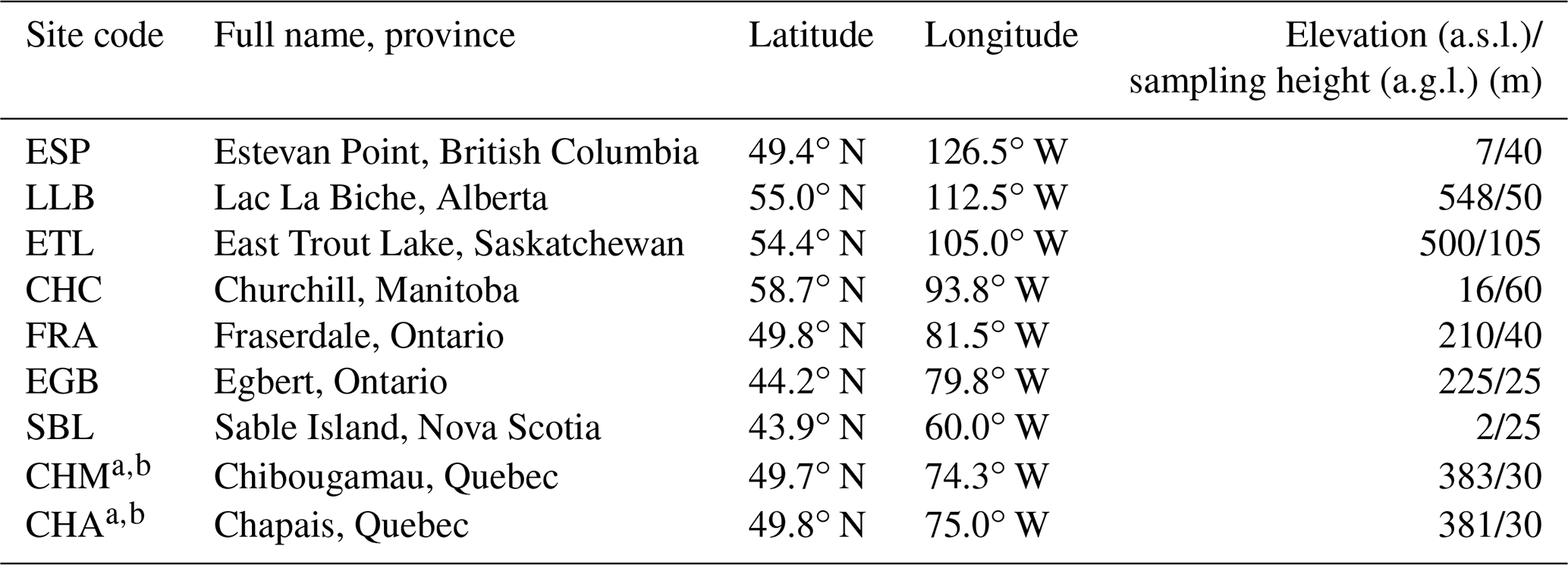
a Chibougamau, Quebec, is replaced by Chapais, Quebec, ∼ 50 km away from 2011 onwards, overlapping in Fig. 1. b Site is used to evaluate the posterior inversion results and is not used in the inversion itself.
2.1.2 GOSAT satellite observations
The Greenhouse Gas Observing Satellite (GOSAT) was launched in January 2009 by the Japan Aerospace Exploration Agency (JAXA). GOSAT is in a low-Earth polar sun-synchronous orbit with an Equator overpass around 13:00 local time. The TANSO-FTS instrument on board GOSAT retrieves column-averaged dry-air mole fractions of methane using short-wave infrared (SWIR) solar backscatter in the 1.65 µm absorption band (Butz et al., 2011). Observation pixels in the default mode are 10 km in diameter separated by 260 km along the orbit track with repeated observations every 3 d. Target-mode observations provide denser spatial coverage over areas of interest. There has been no observed degradation of GOSAT data quality since the beginning of data collection (Kuze et al., 2016). Here we use version 7 of the University of Leicester proxy methane retrieval over land from January 2010 to December 2015 (Parker et al., 2011, 2015; ESA CCI GHG project team, 2018). The single-observation precision of GOSAT XCH4 data is 13 ppb, and the relative bias is 2 ppb when validated against the Total Column Carbon Observing Network (TCCON; Buchwitz et al., 2015). Figure 1 shows the GOSAT observations over Canada used in our analysis within the domain of 45–60∘ N latitude and 50–150∘ W longitude. The observations used have passed all quality assurance flags for a total of 45 936 observations from 2010–2015, or approximately ∼ 7600 observations per year. Our analysis excludes glint data over oceans, and cloudy conditions are accounted for by the quality assurance flags. We avoid using data above 60∘ N latitude due to higher uncertainty in the satellite retrieval and the model comparison (Maasakkers et al., 2019; Turner et al., 2015).
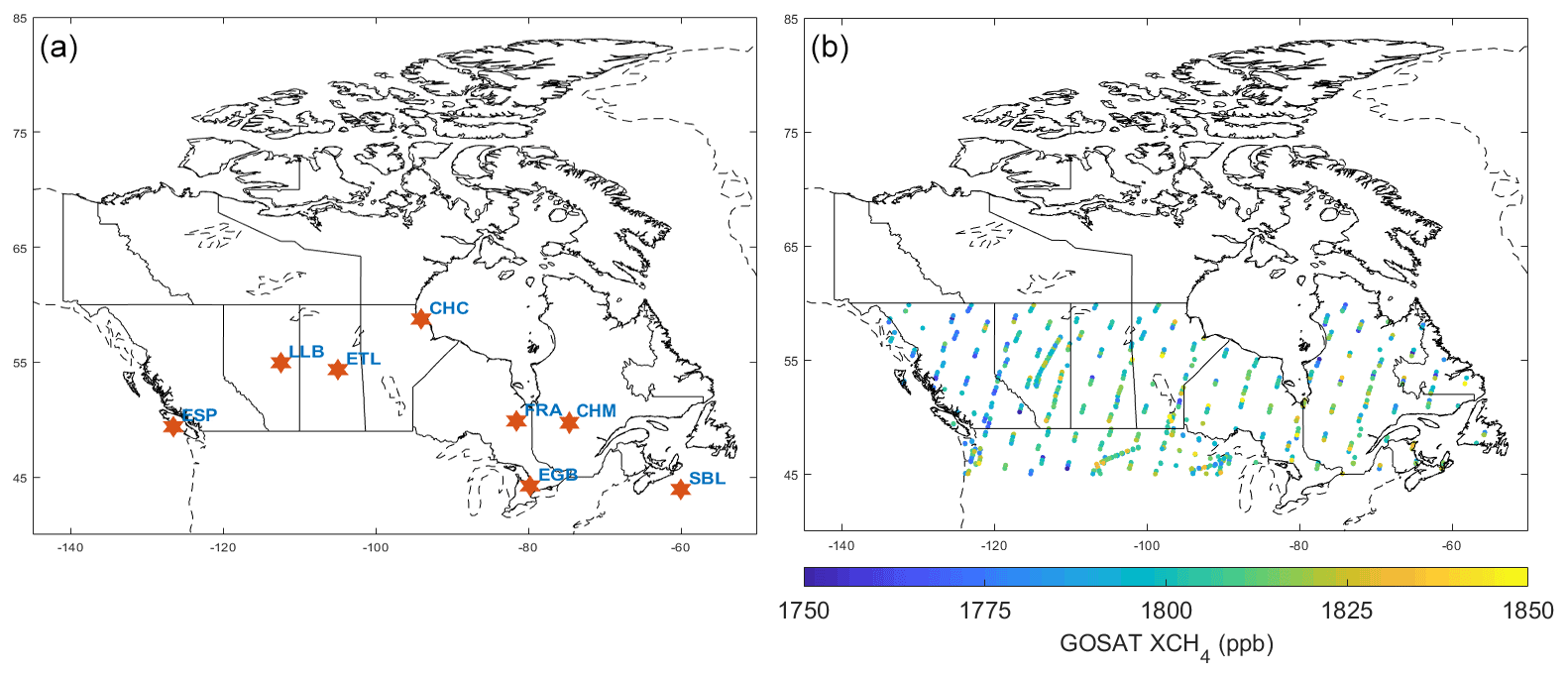
Figure 1ECCC surface (a) and GOSAT satellite (b) observations used in the inverse analysis. A descriptive list of the ECCC sites is shown in Table 1. GOSAT data shown are from a single year in 2013 and are filtered to the Canadian domain within 45–60∘ N latitude and 50–150∘ W longitude. There are ∼ 600 GOSAT observations per month in this domain with a minimum in November–January (112–248) and maximum in July–September (872–1098); individual months are shown in the Supplement (Fig. S1).
2.2 Forward model
We use the GEOS-Chem CTM v12-03 at 2∘ × 2.5∘ grid resolution driven by 2009–2015 MERRA-2 meteorological fields from the NASA Global Modeling and Assimilation Office (GMAO). Initial conditions from January 2009 are from a previous GOSAT inversion by Turner et al. (2015) which was shown to be unbiased globally when compared to surface and aircraft data. Bottom-up anthropogenic emissions in GEOS-Chem are from the 2013 ICF Canadian oil and gas inventory (Sheng et al., 2017) and the 2012 EDGAR v4.3.2 global inventory for other Canadian and global sources and the gridded US 2012 EPA Inventory for the United States (Maasakkers et al., 2016). For wetlands, six configurations from the 2010–2015 extended ensemble of WetCHARTS (Bloom et al., 2017) are used in the ensemble forward model analysis (Sect. 3.1), and the ensemble mean is used as the prior for the inverse analysis (Sect. 3.2–3.4). Figure 2 shows the spatial distribution of the prior methane emissions in Canada from the major anthropogenic and natural sources. The two largest sources are from the ICF oil and gas inventory, (Sheng et al., 2017) and wetland emissions from the ensemble mean of the WetCHARTS inventory (Bloom et al., 2017), with significant emissions from livestock and waste emissions from EDGAR. Oil and gas are 54 % of the anthropogenic total, and wetlands are 94 % of the natural total. The prior emissions estimates in this simulation are summarized in Table 2, which organizes emissions by Canadian source categories and are compared to sector attribution in the National Inventory (Environment and Climate Change Canada, 2017). Our totals for energy, agriculture and waste are 2.4, 1.0 and 0.9 Tg a−1 respectively compared to 2.0, 1.2 and 0.9 Tg a−1 in the National Inventory. In the absence of a spatially disaggregated Canadian inventory for methane, we consider these prior estimates reasonably similar for the purpose of comparing our posterior emissions to the National Inventory; however we cannot compare the spatial pattern of emissions, which will likely show more discrepancies. Natural emissions are divided into wetlands, which are 14.0 Tg a−1 in the ensemble mean, and other natural sources, which are 0.8 Tg a−1 from biomass burning, seeps and termites. Each component of other natural emissions has a separate spatially disaggregated inventory as described in Maasakkers et al. (2019). Emissions from the United States and the rest of the world are included in the model but not optimized in the inversions. Loss of methane from oxidation due to OH is computed using archived 3-D monthly fields of OH from a previous GEOS-Chem full-chemistry simulation (Wecht et al., 2014).
Table 2Mean 2010–2015 prior estimates of Canadian methane emissions used in GEOS-Chem arranged according to categories in the National Inventory (Environment and Climate Change Canada, 2017).

a Emissions inputs for GEOS-Chem. These are shown for the individual source types and summed over the categories energy, agriculture and waste. In Canada, oil and gas are from Sheng et al. (2017); coal, livestock, landfills, wastewater and other anthropogenic are from EDGAR v4.3.2; and wetlands are from Bloom et al. (2017). Biomass burning is from QFED (Darmenov and da Silva, 2013), and termite emissions are from Fung et al. (1991). Seeps and other global sources are described in Maasakkers et al. (2019). b Emissions from the National Inventory (Environment and Climate Change Canada, 2017) that correspond to the energy, agriculture and waste categories. These are used in the discussion of results but are not included in the inverse model.
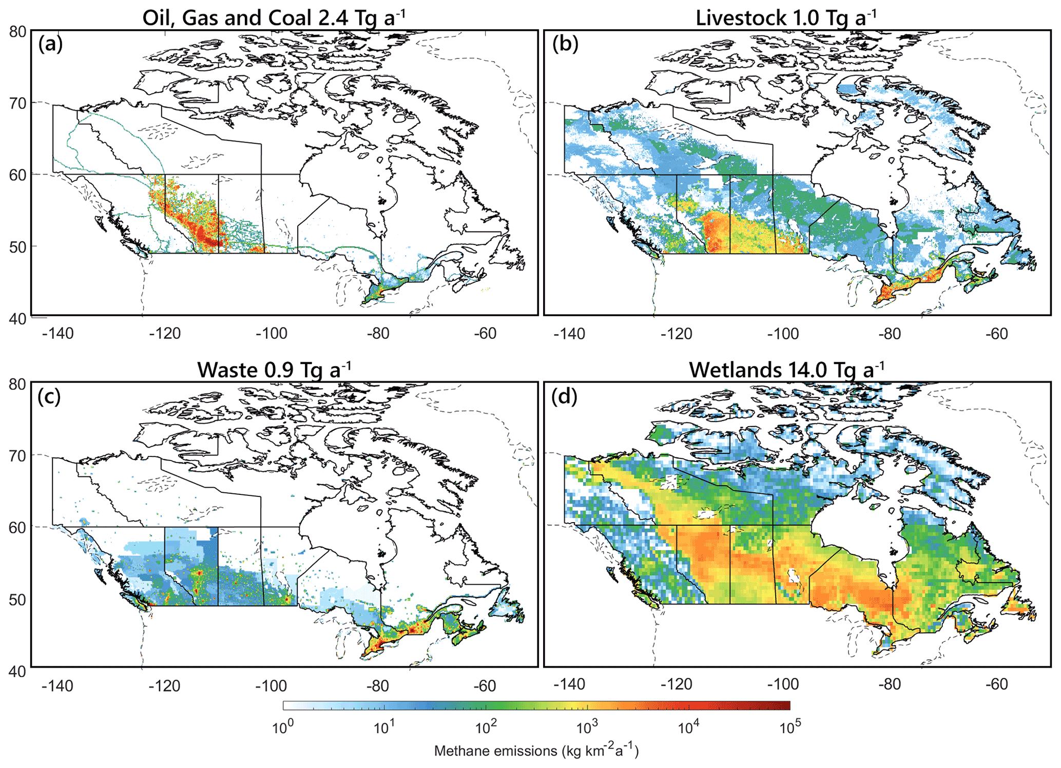
Figure 2Prior estimates of anthropogenic and natural methane emissions. Colour bars are in log scale in units of kilograms of methane per squared kilometre per year (kg CH4 km−2 a−1). Most anthropogenic emissions fall under the energy category (a), which are oil and gas in the ICF inventory (Sheng et al., 2017) plus minor emissions from coal in EDGAR 4.3.2. Livestock (b) and waste (c) are from EDGAR. Natural emissions are primarily wetlands from the WetCHARTS inventory (d; Bloom et al., 2017).
2.3 Inverse model methodology
We optimize emissions in the inverse analysis by minimizing the Bayesian cost function J(x) (Rodgers, 2000).
where x is the vector of emissions being optimized, xa is the vector of prior emissions (Table 2) and F(x) is the simulation of methane concentrations corresponding to the observation vector y of ECCC surface and/or GOSAT data. Sa is the prior error covariance matrix, and So is the observational error covariance matrix. The observational error matrix includes both instrument and model transport error. The GEOS-Chem model relating methane concentrations to emissions F(x) is essentially linear and can be represented by the Jacobian matrix K such that F(x) = Kx+b, where b is the model background. The background includes initial conditions from Turner et al. (2015) and methane from global emissions that are held constant in the inversion. Possible bias in the background is evaluated in detail in the Supplement Sect. S1.3 and shown to be minimal. The K matrix is of m by n size, where n is the number of state vector elements being optimized, and m is the number of ECCC surface and/or GOSAT observations being used. The K matrix is constructed using the forward mode of GEOS-Chem and the tagged tracer output for Canadian sources, which describes the sensitivity of concentrations to emissions in parts per billion per teragram (ppb Tg−1).
GEOS-Chem continuously simulates global emissions with a global source–sink imbalance of +13 Tg a−1 in the budget as described in Maasakkers et al. (2019). We show in Sect. S1.3 of the Supplement that this configuration of the model reliably reproduces the global growth rate in atmospheric methane with adjustments only needed for 2014 and 2015, primarily due to differences in tropical wetland emissions (Maasakkers et al., 2019), with reduced transport errors at 2∘ × 2.5∘ resolution (Stanevich et al., 2020). This gives a well-represented background for methane which is tested using global GOSAT and NOAA data, as well as in situ data at Canadian background sites. We improve the model representation of methane using bias corrections which are discussed in Sect. S1.3 of the Supplement, and we show the consistency of the inversion results without adjustments to the model. A high-resolution inversion over North America over the 2010–2015 time period using the same prior has shown adjustments to US emissions near the Canadian border are also relatively minimal, (Maasakkers et al., 2021), so we treat US emissions as constant. The assumption of constant US emissions is tested in Sect. S1.3.2 of the Supplement by removing ECCC stations near the US border from the inversion, which show consistent results. Hence, we can attribute the model–observation mismatch (y−F(x)) using observations limited to Canada to Canadian emissions which are optimized in the inversion. In the main text we show three inversions with a different number of state vector elements: (a) the monthly inversion (n=78) optimizes monthly natural emissions in Canada and yearly anthropogenic emissions from 2010–2015; (b) the sectoral inversion (n=5) optimizes emissions according to the major inventory categories in Table 2 individually for each year; and (c) the provincial inversion (n=16) optimizes emissions according to subnational boundaries, which is also repeated for each year. The monthly inversion provides higher temporal resolution relative to the other approaches in this study to constrain the seasonality of natural emissions, assuming the spatial distribution is correct. The sectoral inversion provides direct constraints on inventory categories, and the provincial inversion provides relatively higher spatial resolution for subnational attribution. Substituting F(x)=Kx in Eq. (1) and subtracting the background b, the analytical solution of the cost function yields the optimal posterior solution (Rodgers, 2000):
The analytical solution provides closed-form error characterization, such that the posterior error covariance of the posterior solution is given by
The averaging kernel matrix A is used to evaluate the surface and satellite observing systems and is given by
where In is the identity matrix of length n corresponding to the number of state vector elements. The averaging kernel matrix A describes the sensitivity of the posterior solution to the true state x (). The trace of A provides the degrees of freedom for signal (DOFS), which is the number of pieces of information of the state vector that is gained from the inversion (DOFS ≤n). The diagonal values of A provide information on which Canadian state vector elements can be constrained by ECCC surface and GOSAT satellite observations above the noise, and higher DOFS closer to n correspond to better constrained sources in total. As a further diagnostic of the inversion, we conduct a singular value decomposition of the pre-whitened Jacobian (Rodgers, 2000). The number of singular values greater than 1 is the effective rank of K, which shows the independence of the state vector elements and the number of pieces of information above the noise that are resolved in the inversion (Heald et al., 2004). The comparison between this eigenanalysis and the DOFS is discussed in the Supplement Sect. S1.4 and is used to inform the limitations of the observation system.
We construct the prior error covariance matrix Sa based on aggregated error estimates for source categories and regions. We use 50 % error standard deviation for the aggregated anthropogenic emissions, which includes the Sheng et al. (2017) oil and gas inventory and other EDGAR sources, 60 % for wetland emissions from the Bloom et al. (2017) WetCHARTS inventory and 100 % for non-wetlands natural sources. We assume no correlation between state vector elements so that Sa is diagonal. Anthropogenic emissions have been shown to be spatially uncorrelated (Maasakkers et al., 2016); however wetlands show spatial correlation (Bloom et al., 2017). Here we optimize broadly aggregated categories, so our method assumes the spatial pattern of each state vector element is correct; however correlations between state vector elements in the eigenanalysis are used to assess the limitations of source discretization in the observing systems.
We construct the diagonal observation error matrix So, which captures instrument and model error using the relative residual error method (Heald et al., 2004). In this approach the vector of observed–modelled differences is calculated, and the mean observed–modelled difference is attributed to the emissions that will be optimized. Hence, the standard deviation in the residual error represents the observational error and is used as the diagonal elements of So. For our Canadian inversion, we find positive model–observation biases in the warmer months (April to September) and negative biases in the colder months (October to March). We calculate the relative residual error for growing and non-growing seasons separately, such that Δ′ is partitioned into (October to March) and (April to September), which is then used to calculate the diagonal elements of So. For surface observations, the mean observational error is 65 ppb. Since the instrument error is <1 ppb for afternoon mean methane measurements, the observational error is entirely attributed to transport and representation error of surface methane in the model grid pixels. For satellite observations the mean observational error is 16 ppb where the instrument error is 11 ppb, showing most of the observational error is from the instrument rather than the forward model representation of the total column. Column-averaged methane concentrations are less sensitive to surface emissions, resulting in the lower model error (Lu et al., 2021).
In summary, the inverse model is designed to suit the objectives of this study, which are to (1) optimize anthropogenic and natural emissions in Canada at the national scale, (2) compare the results of inversions using surface and satellite observations and (3) characterize the limitations of the observing system towards subnational-scale emissions discretization. The spatial and temporal resolution of the inversion is limited by the precision of GOSAT data, the precision of the model representation of surface methane for ECCC data and the sparse coverage of both systems relative to the smaller magnitude of Canadian emissions. This simplified approach, where Canadian emissions are optimized using only observations in Canada, may be sensitive to errors in the global model that are projected onto the Canadian domain. This is minimized if errors in the regional representation of methane, which are corrected in the inversion, are much larger than errors in the background from the global model or if the background methane is corrected using global observations outside of the Canadian domain. We show an analysis of the global model alongside sensitivity tests of the inversions in Sect. S1.3 of the Supplement, which produce consistent results. Future studies may deploy a more sophisticated, high-resolution inverse model that will match more sophisticated observations, which include an expanded ECCC surface network, as well as satellites with higher density (TROPOMI; Hu et al., 2018) or higher precision (GOSAT-2; Nakajima et al., 2017) observations outside of the years of this analysis.
3.1 Evaluation of WetCHARTS extended ensemble for wetland emissions in Canada
Wetlands are the largest methane source in Canada with uncertainties in the magnitude, seasonality and spatial distribution of emissions. Our inverse analysis constrains the magnitude and seasonality of emissions with observations. Ideally, the prior emissions in the model should be the best possible representation of emissions to reduce error in the optimization problem (Jacob et al., 2016). Table 2 shows 2010–2015 mean wetland emissions in Canada to be 14.0 Tg a−1 from the mean of the WetCHARTS v1.0 inventory (Bloom et al., 2017). These emissions are more than 3 times the total of anthropogenic emissions, 4.4 Tg a−1. The much larger signal from wetland emissions poses a difficulty for constraining anthropogenic emissions (Miller et al., 2014). In this section, we evaluate our use of the mean of the WetCHARTS v1.0 extended ensemble by running a series of forward model runs using alternate ensemble members in GEOS-Chem and comparing model output to ECCC in situ observations.
The WetCHARTS extended ensemble for 2010–2015 contains an uncertainty dataset of 18 possible global wetlands configurations as described in Bloom et al. (2017). These depend on three processing parameters, which are three CH4 : C temperature-dependent respiration fractions (q10=1, 2 and 3, where 1 is the highest temperature dependency), two inundation extent models (GLWD vs. GLOBCOVER, where GLWD corresponds to higher inundation in Canada) and three global scaling factors for global emissions to amount to 124.5, 166 or 207.5 Tg CH4 a−1 (). We find using the scaling factors corresponding to 124.5 and 207.5 Tg CH4 a−1 within GEOS-Chem results in an imbalance in the global budget beyond what is observed in our measurements and degrades the representation of background methane, so we limit the extended ensemble to six members which depend on three temperature parametrizations and two inundation scenarios (). Figure 3 shows the magnitude and spatial distribution of wetland emissions in the six scenarios. The total wetland emissions within Canada show nearly an order of magnitude difference between ensemble members from 3.9 to 32.4 Tg a−1. Compared to the rest of North America, boreal Canada shows the largest variability between ensemble members, with the Southeastern United States as the second most uncertain (Sheng et al., 2018b).
We use ECCC in situ observations to better constrain the range of wetlands methane emissions in the ensemble members. All six configurations are used in GEOS-Chem to produce a series of forward model runs for a subrange of years between 2013–2015. Figure 4 shows GEOS-Chem-simulated methane concentrations using the six WetCHARTS configurations and compares them to four ECCC in situ measurement sites in Canada (LLB, ETL, FRA and EGB). This subset of available data is representative of sites sensitive to both anthropogenic and natural emissions. Most Canadian anthropogenic emissions are from Western Canada (Fig. 2), which we use sites LLB and ETL to evaluate (Fig. 1), and a significant amount of Canadian natural emissions are from regions surrounding the Hudson Bay Lowlands, which we use sites FRA and EGB to evaluate. Methane concentrations from GEOS-Chem show large differences when compared to ECCC observations, ranging from +1050 to −150 ppb. The boundary-condition site ESP (Fig. S3) showed a mean bias of 5.3 ppb for all of 2010–2015. Since there is no similar mismatch in the global representation of methane, these biases up to 1050 ppb can therefore be attributed to misrepresented local Canadian emissions plus associated transport and representation error. Two types of biases with opposite signs appear from this comparison. The first type is a positive summertime bias where the modelled methane concentrations significantly exceed the observations; this bias is more pronounced in sites FRA (Fig. 4c) and EGB (Fig. 4d), which are in Ontario and sensitive to the Hudson Bay Lowlands. The bias is also visible in the western sites LLB (Fig. 4a) and ETL (Fig. 4b) to a lesser extent. As we use a smaller magnitude of wetlands methane emissions corresponding to the ensemble members in Fig. 3 (from 32.4 to 3.9 Tg a−1), this summertime bias decreases proportionately. Therefore, we can attribute these large positive summertime biases to growing season wetland emissions that are overestimated in the process model configurations. The second type of bias is a year-long negative bias that appears most in site LLB (Fig. 4a) and is magnified with the use of lower magnitude wetland emissions. This suggests the presence of year-round anthropogenic emissions in Western Canada that are underestimated in the prior or that wintertime wetland emissions could also be underestimated in WetCHARTS due to the lack of explicit soil water and temperature dependencies. The inverse modelling results in the next section attribute this bias to anthropogenic emissions.
Miller et al. (2016) conducted a study constraining North American boreal wetland emissions from the WETCHIMP inventory modelled in WRF-STILT by a comparison to observations in 2008. Their study included the use of three of the ECCC stations described here (CHM, FRA and ETL). The model comparison to observations in that study showed a similar pattern of modelled methane exceeding observations in the summer and a low bias at ETL. They suggested wetland emissions were overestimated in most model configurations and that the wetlands bias may be masking underestimated anthropogenic emissions. These conclusions are corroborated by the 2013–2015 comparison shown here; we show high wetland emissions configurations in WetCHARTS produce a high bias that exceed measured summertime methane concentrations, and the use of lower wetlands configurations reveal a year-long low bias apparent in Western Canada. Our results suggest the combined use of higher inundation extent and lower temperature dependencies (GLWD and q10=3) or the use of lower inundation extent and higher temperature dependencies (GLOBCOVER and q10=1) best reproduce observations near the mean of the range of emissions, although the ensemble forward model analysis is unable to specify more detailed process model constraints.
The forward model analysis in this section is a direct evaluation of wetlands configurations. This approach allows us to manually tune wetlands scenarios and diagnose the sensitivity of the modelled–observed differences to the process modelling parameters. The inverse analysis shown subsequently is a statistical optimization that applies scaling factors to emissions based on the same model–observation differences. The inverse analysis can be viewed analogously as an automatic approach. These results show the challenge with optimizing Canadian methane emissions when wetland emissions are largely uncertain. Our approach of optimizing anthropogenic and natural emissions simultaneously in an inversion is useful because attempting to constrain either emissions category, anthropogenic or natural, obfuscates the analysis on the other. We exploit the different pattern of anthropogenic and natural emissions in time and space (Fig. 4). Natural emissions peak in the summertime and are concentrated in boreal Canada, while anthropogenic emissions are persistent year-round and are concentrated in Western Canada (Fig. 2). Hence when optimizing the model–observation mismatch in a Bayesian inverse framework, some elements of the observation vector will correspond to high biases from summertime observations in boreal Canada, and some elements will correspond to low biases in Western Canada. As the choice of prior for the inversion, we use the mean of the WetCHARTS configurations (14.0 Tg a−1) which corresponds to the middle of the range shown shaded in red in Fig. 4. The 60 % range of uncertainty in the prior error covariance matrix Sa appropriately excludes the extreme scenarios in Figs. 3 and 4.
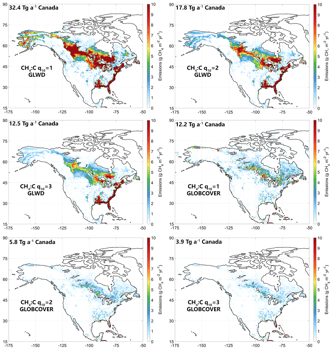
Figure 3Ensemble members from the WetCHARTS v1.0 inventory (Bloom et al., 2017) with totals for wetland methane emissions within Canada for each configuration shown in teragrams of methane per year (Tg CH4 a−1). Ensemble members vary according to the use of three CH4 : C q10 temperature dependencies and two inundation extent scenarios (GLWD vs. GLOBCOVER) for scenarios.
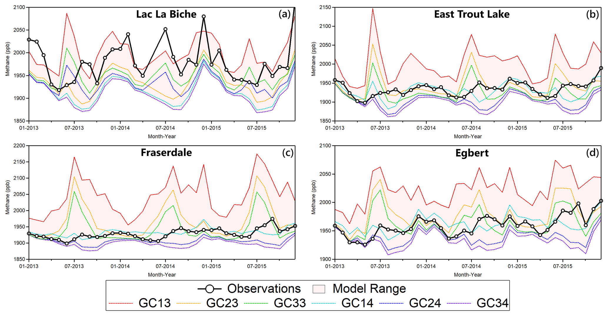
Figure 4Time series of 2013–2015 modelled and observed methane concentrations. Monthly mean methane from ECCC in situ observations (black) are shown and compared to six GEOS-Chem simulations differing in the use of WetCHARTS ensemble members for wetland emissions, with other emissions corresponding to Table 2. The six configurations are labelled GCXY, where the first digit () corresponds to the CH4 : C q10 temperature dependency, which decreases the sensitivity of emissions to temperature with increasing value. The second digit () corresponds to the model used for inundation extent (3 = GLWD, 4 = GLOBCOVER) where GLOBCOVER produces lower emissions in Canada. Emissions configurations are those shown in Fig. 3 in order of magnitude from red to purple lines, with the red shading showing the range of concentrations. Sites are LLB, Alberta (a); ETL, Saskatchewan (b); FRA, Northern Ontario (c); and EGB, Southern Ontario (d).
3.2 Comparative analysis of inversions using ECCC in situ and GOSAT satellite data
We optimize 2010–2015 emissions in Canada using an n=78 state vector element inversion setup with GOSAT and ECCC data independently. Elements 1–72 of the inversion are monthly total natural emissions (wetlands + other natural) from 2010–2015, and elements 73–78 are yearly total anthropogenic emissions (energy + agriculture + waste) for the same years. These categories correspond to the emissions shown in Table 2. We do not optimize emissions according to clustered grid boxes like other satellite inversions using GEOS-Chem (Wecht et al., 2014; Turner et al., 2015; Maasakkers et al., 2019) and instead scale the amplitudes of these two aggregated categories. This approach is a trade-off of time for space, due to the limitations of the observations, giving up finer spatial resolution for finer temporal resolution. This is useful for optimizing Canadian methane emissions since (a) anthropogenic emissions are largely concentrated in Western Canada and require less spatial discretization over the entire country, and (b) natural emissions are the largest source and have an uncertain seasonality – as shown in the previous section – and require finer temporal discretization. The limitations of this method are that natural emissions are very unlikely to be spatially homogenous and vary due to hydrological differences, even at the microtopographic level (Bubier et al., 1993). Perfectly resolving Canadian emissions sources in time and space is challenged by the sparsity and precision of the observing system and the model representation of the observations. We show the limitations of the combined ECCC and GOSAT observing system towards resolving subnational emissions in more detail in the subsequent section.
Figure 5a shows 2010–2015 posterior emissions using this 78 state vector approach with ECCC in situ data (blue) and GOSAT satellite data (green). Error bars are from the diagonal elements of the posterior error covariance matrix . Posterior anthropogenic emissions averaged over the 6 year period are 6.0 ± 0.4 Tg a−1 (1σ year-to-year variability) using ECCC data and 6.5 ± 0.7 Tg a−1 using GOSAT data. Posterior estimates are 36 % and 48 % higher than the prior of 4.4 Tg a−1 for ECCC and GOSAT results, respectively. There does not appear to be a significant year-to-year trend above the noise for the anthropogenic emissions optimized by either dataset. The posterior anthropogenic emissions using ECCC and GOSAT data show agreement with each other in each year but 2011, where the GOSAT derived emissions are statistically higher. The error from the diagonal of the posterior error covariance matrix may be overly optimistic, particularly for GOSAT data. This is due to the observational error covariance matrix So being treated as diagonal when realistically there are correlations between GOSAT observations that are difficult to quantify (Heald et al., 2004). Our results for anthropogenic emissions show agreement with top-down aircraft estimates of methane emissions in Alberta that are higher than bottom-up inventories (Johnson et al., 2017; Baray et al., 2018) and previous satellite inverse modelling studies over North America that upscale emissions in Western Canada (Turner et al., 2015; Maasakkers et al., 2019; Maasakkers et al., 2021; Lu et al., 2021). We show source attribution through a sectoral and subnational-scale analysis of anthropogenic emissions in the subsequent section.
Inversion results for monthly natural emissions from 2010–2015 are also shown in Fig. 5b. The total of posterior natural emissions averaged over the 6-year period is 11.6 ± 1.2 Tg a−1 using ECCC data and 11.7 ± 1.2 Tg a−1 using GOSAT data. The prior for natural emissions is 14.8 Tg a−1 from the mean of the WetCHARTS extended ensemble (14.0 Tg a−1) plus other natural sources (biomass burning + termites + seeps = 0.8 Tg a−1). There is some interannual variability in the prior due to higher emissions in 2010 and 2015. Posterior results averaged over the 6 years are 22 % lower than the prior using ECCC data and 21 % lower using GOSAT data, with both posterior results showing agreement with each other. These results are within the uncertainty range of the WetCHARTS extended ensemble, and we show the magnitude of emissions from the larger uncertainty dataset (3.9 to 32.4 Tg a−1) can be better constrained with both ECCC and GOSAT observations.
While our results show lower natural emissions in all years, a linear fit to the posterior annual emissions using ECCC data shows a trend of increasing natural emissions at a rate of ∼ 0.56 Tg a−1 from 2010–2015. The posterior emissions with GOSAT data do not corroborate this result; the overall emissions trend using GOSAT data is not robust and shows a decreasing trend of ∼ 0.2 Tg a−1. The lack of corroboration of trends between ECCC and GOSAT data may be reflective of the lower overall sensitivity of total column methane to these surface fluxes (Sheng et al., 2017; Lu et al., 2021) or the inability of this inverse system to constrain trends sufficiently. The combined ECCC+GOSAT inversion using this setup is consistent with the results of the individual inversions (shown in the Supplement Fig. S11), while the intercomparison is emphasized here, although we note the combined inversion also does not corroborate this trend. We evaluate the possible influence of errors in the global model on the projection of a trend onto the ECCC inversion in Sect. S1.3.2 of the Supplement. While the mean natural emissions over 2010–2015 show consistent results in the sensitivity tests, the limitations of the observation system, the inversion procedure and the timescale of the analysis limit the interpretation of trends. Poulter et al. (2017) estimated global wetland emissions using biogeochemical process models constrained by inundation and wetlands extend data. They estimated mean annual emissions over all of boreal North America to be 25.1 ± 11.3 Tg a−1 in 2000–2006, 26.1 ± 11.8 Tg a−1 in 2007–2012 and 27.1 ± 12.5 Tg a−1 which suggests a small increasing trend. Observational constraints over longer timescales are necessary to investigate the possibility of trends in Canadian natural methane emissions. Improvements to the observation network and a better understanding of climate sensitivity in WetCHARTS are necessary to understand how wetlands methane emissions will evolve in future climates.
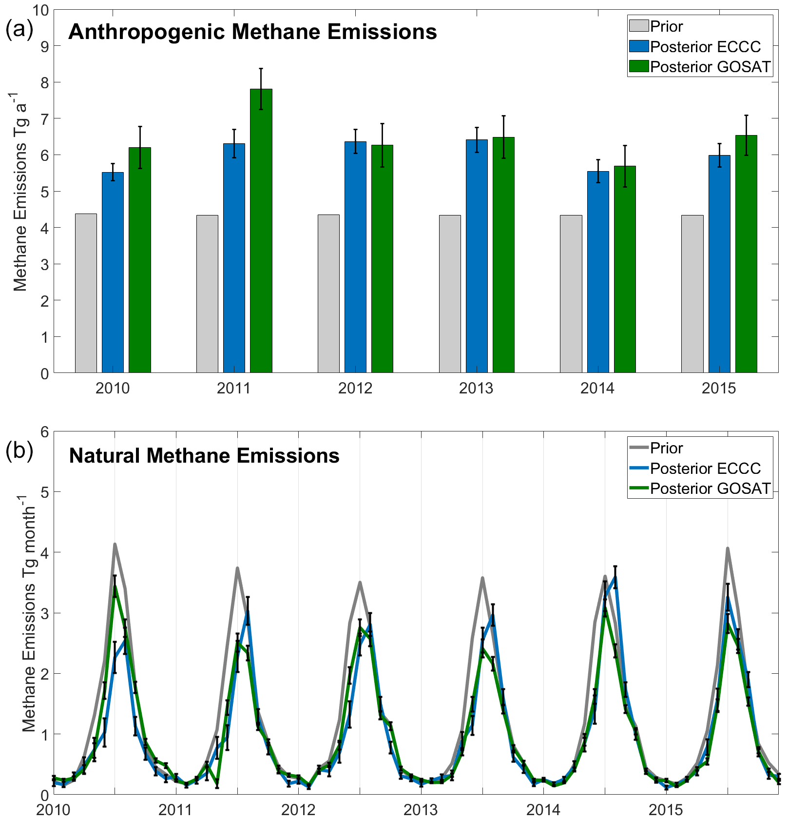
Figure 5Comparative analysis of inversion results optimizing annual total Canadian anthropogenic emissions (a) and monthly total natural emissions (b) in an n=78 state vector element setup. The posterior emissions determined using ECCC in situ (blue) and GOSAT satellite (green) data are compared to the prior (grey). Error bars are from the diagonal elements of the posterior error covariance matrix.
Figure 6 shows the 2010–2015 average seasonal pattern of natural emissions in the prior and posterior results. The seasonality of natural methane emissions in the prior shows a sharp peak in July, with a narrow methanogenic growing season. The posterior emissions with ECCC data shows a peak 1 month later in August in most years instead of July, with emissions lower than the prior in the spring months before the peak (March to May) and similar emissions to the prior in the autumn months after the peak (September to November). Posterior emissions with GOSAT show a peak in July, and this corroborates the pattern of slower to begin spring emissions and the lower intensity summer peak seen from the ECCC inversion. The posterior results show the seasonality of emissions is not symmetrical around the temperature peak in July. August emissions are higher than June, September emissions are higher than May and October emissions are higher than April. This pattern around July is present in the prior emissions from WetCHARTS; however the inversion results constrained by ECCC or GOSAT observations intensify the relative difference between emissions before and after July. Miller et al. (2016) found a similar seasonal pattern of emissions in the Hudson Bay Lowlands using an inverse model constrained by 2007–2008 in situ data. They found a less narrow and less intense peak of summertime emissions with higher emissions in autumn than spring. Warwick et al. (2016) used a forward model and isotopic measurements of δ13C-CH4 and δD-CH4 from 2005–2009 to show northern wetland emissions should peak in August–September with a later spring kick-off and later autumn decline. This is further corroborated by Arctic methane measurements (Thonat et al., 2017) and high-latitude eddy covariance measurements (Peltola et al., 2019; Treat et al., 2018; Zona et al., 2016) that show a larger contribution from the non-growing season. Our inverse model results using ECCC and GOSAT data both show agreement with slower to start emissions in the spring and a less intense summertime peak for Canadian wetland emissions.
Several mechanisms have been proposed to describe a larger relative contribution from cold-season methane emissions. Pickett-Heaps et al. (2011) attributed a delayed spring onset in the HBL to the suppression of emissions by snow cover. The temperature dependency in WetCHARTS is based on surface skin temperature (Bloom et al., 2017); however subsurface soil temperatures may continue to sustain methane emissions while the surface is below freezing. When subsurface soil temperatures are near 0 ∘C, this “zero curtain” period can further continue to release methane for an extended period (Zona et al., 2016). Subsurface soils may remain unfrozen at a depth of 40 cm, even until December (Miller et al., 2016). Alternatively, field studies in the 1990s suggested the seasonality of emissions may be more influenced by hydrology than temperature, with large differences between peatlands sites (Moore et al., 1994). The WetCHARTS extended ensemble inundation extent variable is constrained seasonally by precipitation. While this does not directly constrain water table depth and wetland extent, it provides an aggregate constraint on hydrological variability (Bloom et al., 2017). We show the mean seasonal pattern of both air temperature and precipitation from climatological measurements in subarctic Canada are similarly asymmetrical about the July peak (Fig. S2 in the Supplement). August is warmer and wetter than June, September is warmer and wetter than May and October is wetter and warmer than April – with wetness being more persistent into the autumn than air temperature. Our inversion results showing a delayed spring start in the seasonal pattern of natural methane emissions in Canada may suggest a lag in the response of methane emissions to temperature and precipitation. This may be due to lingering subsurface soil temperatures and/or more complex parametrization necessary for hydrology.
The overall agreement between ECCC and GOSAT inversions shows robustness in the results. While the same model, prior emissions and inversion procedure are used for assimilating ECCC and GOSAT data, the two datasets are produced with very different measurement methodologies (in situ vs. remote sensing) and sample different parts of the atmosphere (surface concentrations or the total vertical column). The posterior error intervals shown from reflect assumptions about the treatment of observations and may insufficiently account for correlations; however the comparative analysis provides a useful sensitivity test of the posterior emissions since the datasets reflect different treatment of these assumptions.
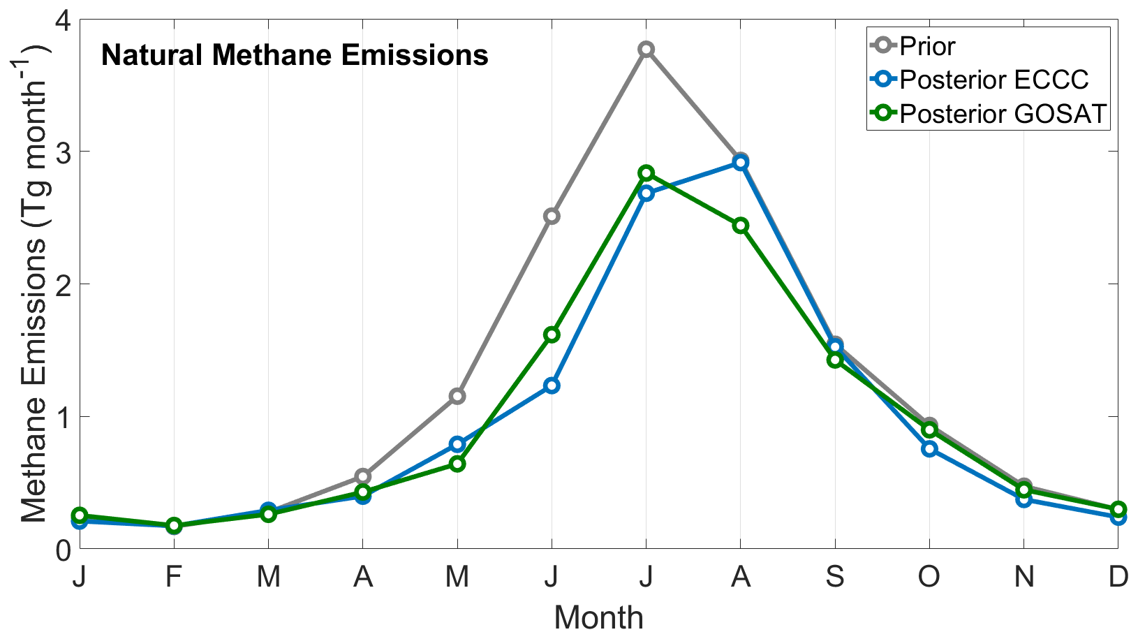
Figure 6Mean 2010–2015 seasonal pattern of natural methane emissions in teragrams per month. The annual total emissions are 14.8 (prior, grey), 11.6 ± 1.2 (posterior ECCC, blue) and 11.7 ± 1.2 Tg a−1 (posterior GOSAT, green). The posterior results are within the uncertainty range provided by the WetCHARTS extended ensemble (3.9–32.4 Tg a−1 for Canada).
3.3 Joint inversions combining ECCC in situ and GOSAT satellite data
We combine the ECCC and GOSAT datasets in two policy-themed inversions: (1) optimizing emissions according to the sectors in the national inventory (n=5 state vector elements; corresponding to the categories in Table 2) and (2) optimizing emissions by provinces split into anthropogenic and natural totals (n=16), and we show the results in Fig. 7. These inversions are underdetermined and show the limitations of the ECCC+GOSAT observing system towards constraining emissions in Canada with very small magnitudes. We conduct the inversions for each year from 2010–2015 individually and present the average from these six samples. Since these two policy inversions use a low number of state vector elements, they are vulnerable to both aggregation error and overfitting of the well-constrained state vector elements and do not necessarily benefit from using a larger data vector from all 6 years. We discuss the diagnostics and information content for these inversions in detail in Sect. S1.4 of the Supplement. The error bars are the 1σ standard deviation of the six yearly results and therefore represent both noise in the inversion procedure and year-to-year differences in the state (emissions and/or transport). Here we do not apply a weighting factor to either dataset; the observations are treated equivalently for the cost function in Eq. (1). While there are about 5 times more GOSAT observations than ECCC observations for use in the analysis, and the in situ observations have larger observational error in Sa (due to model error), the surface measurements are much more sensitive to surface fluxes, which offsets the weight of the larger amount of GOSAT data. As further diagnostics, we show the inversions using GOSAT and ECCC individually (Tables S4 and S5), which show general agreement between the datasets. We also use a singular value decomposition eigenanalysis (Heald et al., 2004) to evaluate the independence of the state vector elements and to demonstrate which sectoral categories and provinces can be reliably constrained above the noise in the system (Fig. S9 and S10 in the Supplement).
Figure 7a shows the sectoral inversion corresponding to categories in the National Inventory (Table 2). The prior emissions with 50 % error estimates (60 % for wetlands) are 2.4 (energy), 1.0 (agriculture), 0.9 (waste), 14.0 (wetlands) and 0.8 Tg a−1 (other natural). the posterior emissions are 3.6 ± 0.9 (energy), 1.5 ± 0.4 (agriculture), 0.8 ± 0.2 (waste), 9.6 ± 1.1 (wetlands) and 1.7 ± 0.9 Tg a−1 (other natural). The degrees of freedom for signal and singular value decomposition (Fig. S9) show three to four independent pieces of information can be retrieved, which are differentiated in the figure by solid and hatched bars. The singular value decomposition shows strong source signals corresponding to wetlands and energy, with signal-to-noise ratios of ∼ 37 and ∼ 5, respectively. These are the two largest emissions sources in Canada and show the inverse system can successfully disentangle the major anthropogenic and natural contributors. Emissions from waste have a signal-to-noise ratio of ∼ 2 and can be constrained despite the low magnitude of emissions. This is likely due to waste emissions being more concentrated in Central Canada and away from the influence of large energy and agriculture emissions in Western Canada. Emissions from other natural sources are at the noise limit and show a moderate correlation with wetlands, which shows that these two sources are not completely independent. Agriculture emissions are below the noise in the system and highly correlated with energy emissions. This is likely due to the high spatial overlap of energy and agriculture emissions in Western Canada. As a result of these limitations, we present the total of energy and agriculture as 5.1 ± 1.0 Tg a−1 and the total of wetlands and other natural as 11.3 ± 1.4 Tg a−1. Our results for total natural and total anthropogenic emissions are consistent with the results from the previous monthly inversion, with the added benefit of identifying which sectors are responsible for the higher anthropogenic emissions at the cost of lower temporal resolution. Waste emissions are 15 % lower than the prior and 14 % lower than the National Inventory. The total for energy and agriculture is 49 % higher than the prior and 59 % higher than the total in the inventory. These results show that energy and/or agriculture are the sectors that are responsible for the higher anthropogenic emissions.
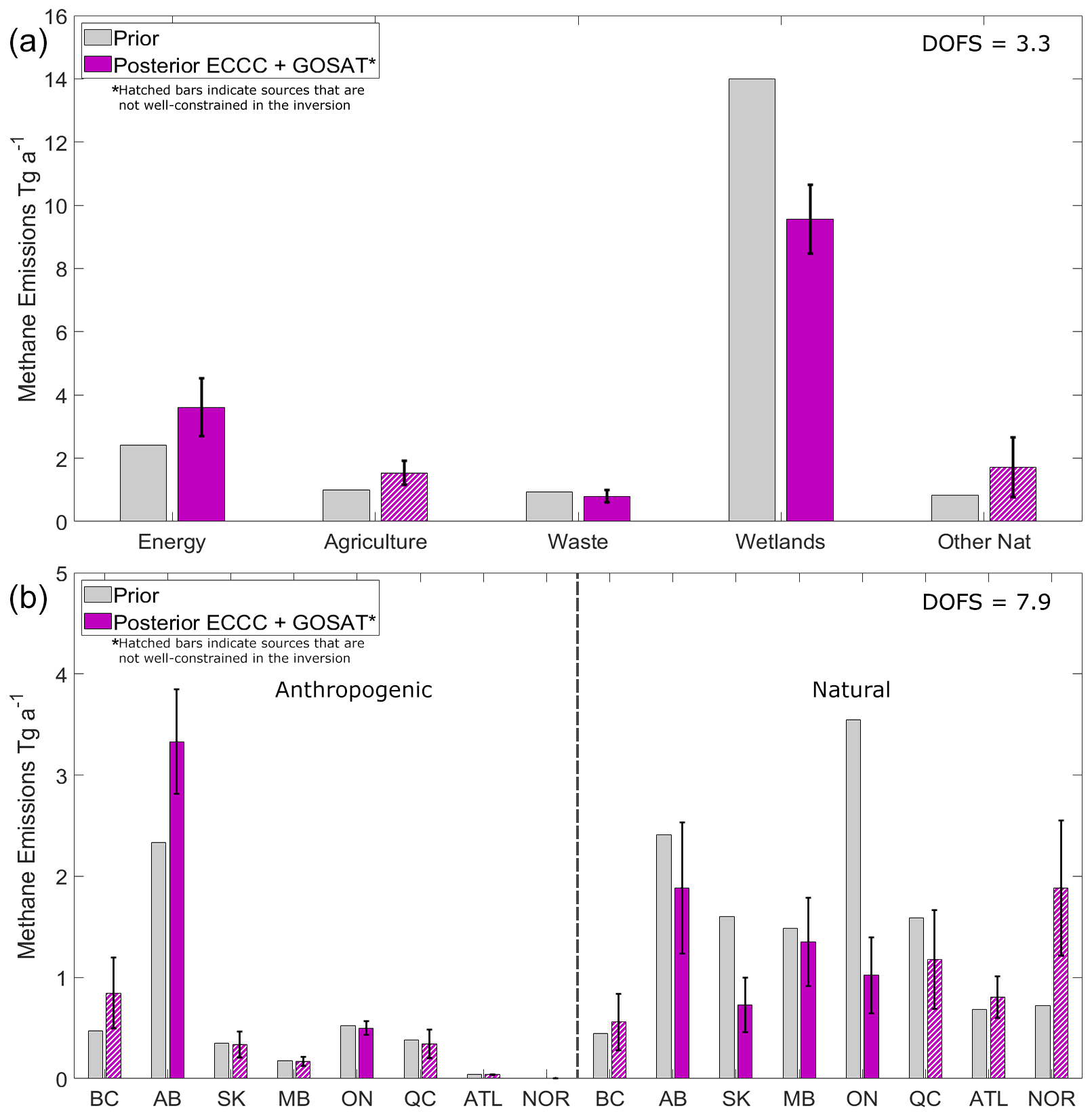
Figure 7Joint inversions combining 2010–2015 ECCC in situ and GOSAT satellite data showing how the combined observing system remains limited towards resolving all Canadian sources. Inversions are done for each year, and we present the 6-year average with error bars showing the 1σ standard deviation of the yearly results. Hatched bars indicate sources that are not well constrained; these are defined as state vector elements with averaging kernel sensitivities less than 0.8 which are affected by aliasing with other sources (see Supplement Figs. S9 and S10). Panel (a) shows the sectoral inversion according to the categories in the National Inventory (energy, agriculture and waste) and two natural categories (wetlands and other natural). As an example, the diagnostics in Fig. S9 show agriculture emissions are beneath the noise and cannot be distinguished from energy. Panel (b) shows the subnational regional inversion according to provinces (BC British Columbia, AB Alberta, SK Saskatchewan, MB Manitoba, ON Ontario and QC Quebec) and aggregated regions (ATL Atlantic Canada and NOR Northern Territories) further subdivided according to total anthropogenic and total natural emissions. The diagnostics in Fig. S10 show more than half of the regions are at or below the noise. For anthropogenic emissions, the best constraints are on provinces AB and ON. For natural emissions, the best constraints are on AB, SK, MB and ON.
Figure 7b shows the provincial inversion corresponding to the six largest emitting provinces (BC British Columbia, AB Alberta, SK, Saskatchewan, MB Manitoba, ON Ontario and QC Quebec) and two aggregated regions (ATL Atlantic Canada and NOR Northern Territories). These regions are further subdivided into total anthropogenic and total natural methane emissions, with below-detection-limit anthropogenic emissions from Atlantic Canada and Northern Territories. This inversion especially challenges the limitations of the ECCC + GOSAT observation system, as only about 8 of 16 independent pieces of information are retrieved. This means that half of the posterior provincial emissions are below the noise, and we are unable to constrain province-by-province emissions. The singular value decomposition identifies which regions are well constrained (Fig. S10). For the anthropogenic emissions, AB and ON are strongly constrained. For the natural emissions, AB, ON, SK and MB are well constrained. BC shows correlation between its own anthropogenic and natural emissions and cannot be completely disaggregated. As a result, we group elements together in Western Canada (BC + AB + SA + MB) and Central Canada (ON + QC) for interpretation. The total for Western Canada anthropogenic emissions is 4.7 ± 0.6 Tg a−1, which is 42 % higher than the prior of 3.3 Tg a−1. The total for Central Canada is 0.8 ± 0.2 Tg a−1, which is 11 % lower than the prior of 0.9 Tg a−1.
Each of our top-down inversion results show higher total anthropogenic emissions than bottom-up estimates. This is consistent regardless of the observation vector incorporating ECCC data, GOSAT data or ECCC + GOSAT data. The subnational-scale emissions are limited in their ability to provide full characterization of minor emissions across Canada but can successfully constrain major emissions for source attribution. The sectoral inversion attributes higher anthropogenic emissions to energy and/or agriculture and applies a small decrease to waste emissions. The provincial inversion attributes higher anthropogenic emissions to Western Canada and a small decrease to Central Canada. These results suggest that anthropogenic emissions in Canada are underestimated primarily because of higher emissions from Western Canada energy and/or agriculture. This interpretation is consistent with previous satellite inverse modelling studies over North America that apply positive scaling factors to grid box clusters in Western Canada to match observations (Maasakkers et al., 2019; Turner et al., 2015; Wecht et al., 2014). Aircraft studies in Alberta have also shown higher emissions from oil and gas in Alberta than bottom-up estimates (Baray et al., 2018; Johnson et al., 2017). Atherton et al. (2017) estimated higher emissions from natural gas in north-eastern British Columbia using mobile surface in situ measurements (Atherton et al., 2017). Zavala-Araiza et al. (2018) showed a significant amount of methane emissions in Alberta from equipment leaks and venting go unreported due to current reporting requirements, and in some regions a small number of sites may be responsible for most methane emissions. Our inverse modelling results from 2010–2015 suggest a consistent presence of under-reported or unreported emissions which require a policy adjustment to reporting practices.
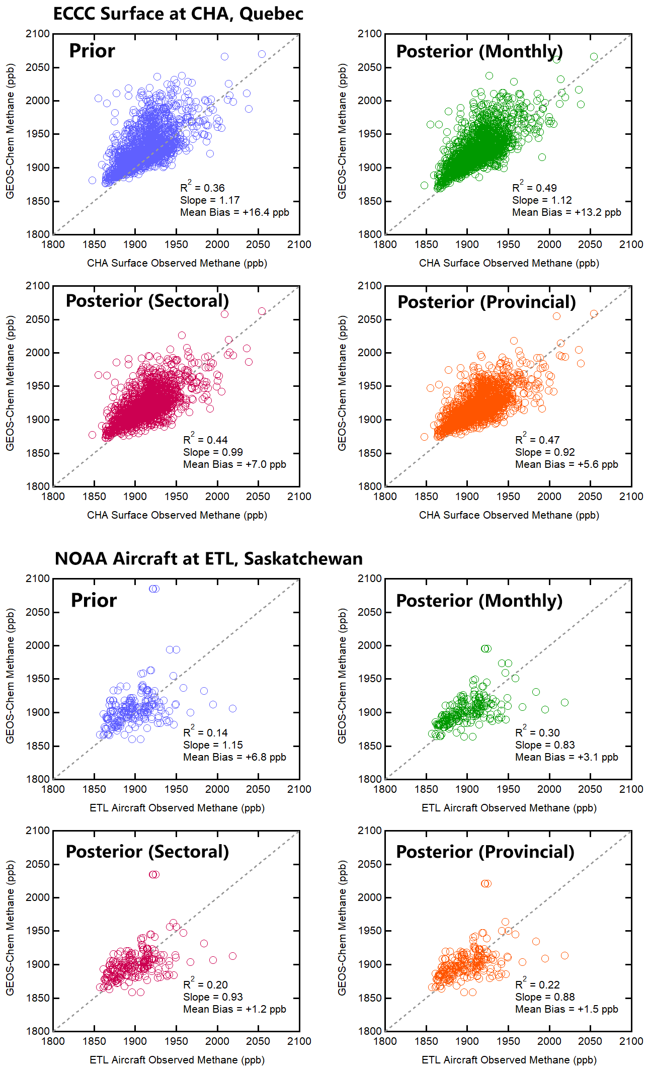
Figure 8Evaluation of inversion results with reduced major axis (RMA) regressions using independent data. The top four panels show the comparison to ECCC surface observations at Chapais and Chibougamau in Quebec, Canada, and the bottom four panels show the comparison to NOAA aircraft profiles at East Trout Lake, Saskatchewan. The agreement of observations with prior simulated methane concentrations (blue) is compared to posterior concentrations using optimized emissions from the monthly inversion (green), the sectoral inversion (magenta) and the provincial inversion (orange). The coefficient of determination (R2), slope and mean bias are shown as metrics of agreement.
3.4 Comparison to independent aircraft and in situ data
We test the robustness of the optimized emissions from each of the three inversions shown (monthly natural, sectoral and provincial) by a comparison to independent measurements not used in the inversions. Prior and posterior simulated methane concentrations are compared to measurements from NOAA ESRL aircraft profiles at East Trout Lake, Saskatchewan (Mund et al., 2017), and ECCC surface measurements in sites Chapais and Chibougamau in Quebec, Canada. The surface data were averaged to daily afternoon means (12:00 to 16:00 local time) in the same manner as the surface measurements used in the inversion. Aircraft data from the NOAA ESRL profiles coincide spatially with the surface measurements at ETL through a joint analysis program with Environment and Climate Change Canada and have occurred on a regular basis approximately once a month from 2005 until present time. Aircraft measurements reach ∼ 7000 m above the surface with samples at multiple altitudes accomplished using a programmable multi-flask system that is further discussed in Mund et al. (2017); however we limit the comparison to the lowest 1 km above ground since higher altitude measurements are mostly background. The aircraft data are not averaged; however the flights occur around the same time in the early afternoon.
Figure 8 shows the comparison using reduced major axis (RMA) regression, with the coefficient of determination (R2), the slope and the mean bias shown as metrics to evaluate the agreement. Surface data in CHA, Quebec, show better posterior agreement with observations according to all metrics for each of the three inversions. The R2 of the prior is 0.36 and improves to a range of 0.44–0.49 for the posterior results, the slope is 1.17 in the prior and improves to a range of 0.92–1.12 and the mean bias (model – observations) is +16.4 ppb in the prior and improves to +13.2 and +5.6 ppb. Since this site in Quebec is particularly sensitive to the Hudson Bay Lowlands, the agreement in all metrics suggests our posterior emissions can better represent wetland emissions in this region. This includes the reduced peak seasonality of natural emissions in the monthly inversion, the reduction of wetland emissions in the sectoral inversion and the reduction of natural emissions primarily in Central Canada in the provincial inversion. Aircraft data in Saskatchewan show improvement in the R2 and mean bias metrics, but the slope slightly degrades in one case. The R2 of the prior is 0.14 and improves to a range of 0.20–0.30, and the mean bias of the prior is +6.8 ppb and improves to +1.2 and +3.1 ppb. The slope of the prior is 1.15, which slightly degrades to 0.83 in the monthly inversion and improves to a range of 0.88–0.93 in the provincial and sectoral inversions. The high-resolution aircraft measurements are more susceptible to representation error at this 2∘ × 2.5∘ grid resolution. Furthermore, the time-series comparison to surface data at East Trout Lake (Fig. 4) shows overall lower sensitivity to summertime wetland emissions than Fraserdale and Egbert and lower sensitivity to anthropogenic emissions from Alberta than Lac La Biche. Hence, the modelled methane concentrations at the aircraft measurement points are adjusted less by the change in posterior emissions. However, improvement in the R2 and mean bias metrics shows there is still a better representation of the variance in the data, which suggests the posterior emissions reduce bias due to peak emission episodes.
We conduct a Bayesian inverse analysis to optimize anthropogenic and natural methane emissions in Canada using 2010–2015 ECCC in situ and GOSAT satellite observations in GEOS-Chem. Methane concentrations are simulated on a 2∘ × 2.5∘ grid using recently updated prior emissions inventories for energy and wetland emissions in Canada. Modelled background conditions for the Canadian domain are shown to be unbiased in the comparison to surface in situ data at the westernmost site in Canada, Estevan Point, with agreement within 6 ppb. A forward model analysis shows much larger biases between −100 ppb and +1050 ppb at surface sites throughout Canada, demonstrating the presence of misrepresented local emissions. We show large positive biases (overestimation of emissions) in the summertime are observed at sites sensitive to wetland emissions; these biases are reduced by using lower magnitude wetland emissions scenarios with lower CH4 : C temperature sensitivities or lower inundation extent. We also show the opposite case of negative biases (underestimation of emissions) observed year-round at sites in Western Canada. The forward model analysis is consistent with the results of the inverse analysis that reduce emissions from natural sources and increase emissions from anthropogenic sources to minimize the mismatch between modelled and observed methane.
We show three approaches for using ECCC and GOSAT data towards inverse modelling of Canadian methane emissions. These approaches differ according to the temporal and spatial resolution of the solution. We show (1) a relatively higher time-resolution inversion that solves for natural emissions each month from 2010–2015 and anthropogenic emissions as yearly totals, (2) a sectoral inversion that solves for emissions according to categories in the National Inventory and (3) a provincial inversion that solves for total anthropogenic and natural emissions at the subnational level. The monthly inversion provides information on the seasonality of natural emissions (which are ∼ 95 % wetlands) but does not provide more depth into anthropogenic emissions beyond yearly scaling. The sectoral inversion provides more information on the categories of anthropogenic emissions that are misrepresented in the prior but without spatial detail. The provincial inversion provides the highest level of spatial discretization but is largely underdetermined due to the limitations of the observing system towards characterizing very low magnitude emissions from smaller contributing provinces.
Inversion results show mean 2010–2015 posterior emissions for total anthropogenic sources in Canada are 6.0 ± 0.4 Tg a−1 using ECCC data and 6.5 ± 0.7 Tg a−1 using GOSAT data. Annual mean natural emissions are 11.6 ± 1.2 Tg a−1 using ECCC data and 11.7 ± 1.2 Tg a−1 using GOSAT data. Both inverse modelling estimates are higher than the prior for anthropogenic emissions, 4.4 Tg a−1, and lower than the prior for natural emissions, 14.8 Tg a−1. Inversion results using both datasets show a change in the seasonal profile of natural methane emissions, where emissions are slower to begin in the spring and show a less intense peak in the summer. The agreement between two datasets assembled with different measurement methodologies that sample different parts of the atmosphere is a robust result that lends weight to our conclusions. Our results corroborate recent studies showing a less intense and less narrow summertime peak in North American boreal wetland emissions, with a higher relative contribution from the cold season (Miller et al., 2016; Zona et al., 2016; Warwick et al., 2016; Thonat et al., 2017; Treat et al., 2018; Peltola et al., 2019). These top-down studies using atmospheric observations show biosphere process models can better account for a more complex response to peak surface soil temperatures.
We also conduct combined ECCC + GOSAT inversions that aim to resolve finer resolution emissions corresponding to the sectors of the National Inventory and corresponding to provincial boundaries. These policy-themed inversions challenge the capabilities of the ECCC+GOSAT observation system and show the system is not capable of resolving many minor emissions in Canada. The degrees of freedom for signal for these inversions are 3–4 out of 5 state vector elements for the sectoral inversion and 8 out of 16 for the provincial inversion. The limitation of this inverse approach towards constraining sectoral or regional-scale emissions in Canada is due to the low magnitude of these emissions, their overlapping nature in concentrated regions and the sparsity of data available to distinguish them apart. Grouping correlated sectors together, we determine 5.1 ± 1.0 Tg a−1 for energy and agriculture, which is 59 % higher than the inventory, and 0.8 ± 0.2 Tg a−1 for waste, which is 14 % lower than the inventory. For provincial emissions, we show Western Canada is 4.7 ± 0.6 Tg a−1, which is 42 % higher than the prior, and Central Canada is 0.8 ± 0.2, which is 11 % lower. Both regions show lower natural emissions. These results show that the higher anthropogenic emissions in the posterior results can be attributed to energy and/or agriculture primarily in Western Canada where most of Canadian anthropogenic emissions are concentrated. Our results are consistent with other top-down studies that show higher anthropogenic emissions than reported in Western Canada (Wecht et al., 2014; Turner et al., 2015; Atherton et al., 2017; Johnson et al., 2017; Baray et al., 2018; Maasakkers et al., 2019). This may be due to oil and gas emissions that are under-reported or unreported due to current reporting requirements (Zavala-Araiza et al., 2018). These top-down studies show a need for policy readjustment in reporting practices for Canadian anthropogenic methane emissions.
This study shows the value of using complementary surface and satellite datasets in an inverse analysis. We emphasize the value of comparative analysis using the datasets independently versus as joint inversions, as minor emissions are too low in magnitude for the observational precision to distinguish finer scale discretization above the noise. The comparative analysis has the added benefit of evaluating the datasets against each other and the assumptions that are specific to using either surface or satellite data. The capabilities for combining and intercomparing datasets are expected to improve with the launch of Copernicus Sentinel-5P satellite (TROPOMI) in 2017 and continued expansions of in situ observation networks. The ability for next-generation observations to constrain subnational-level emissions in Canada will depend on instrument and model precision, as well as the emissions magnitudes and spatiotemporal overlap of the targets. These technical capabilities should be weighed alongside policy needs for improved methane monitoring.
GEOS-Chem is from https://doi.org/10.5281/zenodo.1464210 (last access: 1 April 2019; The International GEOS-Chem User Community, 2018), which includes links to all gridded prior emissions and meteorological fields used in this analysis. GOSAT satellite data are from the University of Leicester v7 proxy retrieval, available through the ESA Greenhouse Gases Climate Change Initiative: https://catalogue.ceda.ac.uk/uuid/f9154243fd8744bdaf2a59c39033e659 (last access: 1 July 2021; ESA CCI GHG project team, 2018). ECCC in situ data are available through the World Data Centre for Greenhouse Gases (WDCGG) at https://gaw.kishou.go.jp/ (last access 1 July 2021; WDCGG, 2018). NOAA/ESRL aircraft data are from the Global Monitoring Laboratory at https://doi.org/10.7289/V5N58JMF (last access 1 July 2021; Mund et al., 2017).
The supplement related to this article is available online at: https://doi.org/10.5194/acp-21-18101-2021-supplement.
SB, DJJ and RM designed the study. SB conducted the simulations and analysis with contributions from JDM, JXS, MPS and DBAJ. AAB provided WetCHARTS emissions and supporting data. SB and RM wrote the paper with contributions from all authors.
The authors declare that they have no conflict of interest.
Publisher’s note: Copernicus Publications remains neutral with regard to jurisdictional claims in published maps and institutional affiliations.
Work at Harvard was supported by the NASA Carbon Monitoring System. We thank the Japanese Aerospace Exploration Agency (JAXA), responsible for the GOSAT instrument, and the University of Leicester for the retrieval algorithm used in this analysis. Doug Worthy and the Climate Research Division at Environment and Climate Change Canada are responsible for the in situ surface measurements, and the NOAA/ESRL/GML program is responsible for the Carbon Cycle Greenhouse Gases (CCGG) cooperative air sampling network measurements.
This research has been supported by the Natural Sciences and Engineering Research Council of Canada (grant nos. RGPIN-2018-05898 and 398061-201).
This paper was edited by Patrick Jöckel and reviewed by Julia Marshall and one anonymous referee.
Atherton, E., Risk, D., Fougère, C., Lavoie, M., Marshall, A., Werring, J., Williams, J. P., and Minions, C.: Mobile measurement of methane emissions from natural gas developments in northeastern British Columbia, Canada, Atmos. Chem. Phys., 17, 12405–12420, https://doi.org/10.5194/acp-17-12405-2017, 2017.
Baray, S., Darlington, A., Gordon, M., Hayden, K. L., Leithead, A., Li, S.-M., Liu, P. S. K., Mittermeier, R. L., Moussa, S. G., O'Brien, J., Staebler, R., Wolde, M., Worthy, D., and McLaren, R.: Quantification of methane sources in the Athabasca Oil Sands Region of Alberta by aircraft mass balance, Atmos. Chem. Phys., 18, 7361–7378, https://doi.org/10.5194/acp-18-7361-2018, 2018.
Bloom, A. A., Bowman, K. W., Lee, M., Turner, A. J., Schroeder, R., Worden, J. R., Weidner, R., McDonald, K. C., and Jacob, D. J.: A global wetland methane emissions and uncertainty dataset for atmospheric chemical transport models (WetCHARTs version 1.0), Geosci. Model Dev., 10, 2141–2156, https://doi.org/10.5194/gmd-10-2141-2017, 2017.
Bubier, J. L., Moore, T. R., and Roulet, N. T.: Methane Emissions from Wetlands in the Midboreal Region of Northern Ontario, Canada, Ecology, 74, 2240–2254, https://doi.org/10.2307/1939577, 1993.
Buchwitz, M., Reuter, M., Schneising, O., Boesch, H., Guerlet, S., Dils, B., Aben, I., Armante, R., Bergamaschi, P., Blumenstock, T., Bovensmann, H., Brunner, D., Buchmann, B., Burrows, J. P., Butz, A., Chédin, A., Chevallier, F., Crevoisier, C. D., Deutscher, N. M., Frankenberg, C., Hase, F., Hasekamp, O. P., Heymann, J., Kaminski, T., Laeng, A., Lichtenberg, G., De Mazière, M., Noël, S., Notholt, J., Orphal, J., Popp, C., Parker, R., Scholze, M., Sussmann, R., Stiller, G. P., Warneke, T., Zehner, C., Bril, A., Crisp, D., Griffith, D. W. T., Kuze, A., O'Dell, C., Oshchepkov, S., Sherlock, V., Suto, H., Wennberg, P., Wunch, D., Yokota, T., and Yoshida, Y.: The Greenhouse Gas Climate Change Initiative (GHG-CCI): Comparison and quality assessment of near-surface-sensitive satellite-derived CO2 and CH4 global data sets, Remote Sens. Environ., 162, 344–362, https://doi.org/10.1016/j.rse.2013.04.024, 2015.
Butz, A., Guerlet, S., Hasekamp, O., Schepers, D., Galli, A., Aben, I., Frankenberg, C., Hartmann, J.-M., Tran, H., and Kuze, A.: Toward accurate CO2 and CH4 observations from GOSAT, Geophys. Res. Lett., 38, L14812, https://doi.org/10.1029/2011GL047888, 2011.
Darmenov, A. and da Silva, A.: The quick fire emissions dataset (QFED) – documentation of versions 2.1, 2.2 and 2.4, NASA Technical Report Series on Global Modeling and Data Assimilation, NASA TM-2013-104606, 32, 183 pp., 2013.
Environment and Climate Change Canada: National Inventory Report 1990–2015: Greenhouse Gas Sources and Sinks in Canada, Canada's Submission to the United Nations Framework Convention on Climate Change, Part 3, available at: http://publications.gc.ca/collections/collection_2018/eccc/En81-4-2015-3-eng.pdf (last access: 7 November 2020), 2017.
ESA CCI GHG project team: ESA Greenhouse Gases Climate Change Initiative (GHG_cci): Column-averaged CH4 from GOSAT generated with the OCPR (UoL-PR) Proxy algorithm (CH4_GOS_OCPR), v7.0. Centre for Environmental Data Analysis, available at: https://catalogue.ceda.ac.uk/uuid/f9154243fd8744bdaf2a59c39033e659 (last access: 1 July 2021), 2018.
Fung, I., John, J., Lerner, J., Matthews, E., Prather, M., Steele, L. P., and Fraser, P. J.: Three-dimensional model synthesis of the global methane cycle, J. Geophys. Res., 96, 13033, https://doi.org/10.1029/91JD01247, 1991.
Hartmann, D. L., Tank, A. M. K., Rusticucci, M., Alexander, L. V., Brönnimann, S., Charabi, Y. A. R., Dentener, F. J., Dlugokencky, E. J., Easterling, D. R., Kaplan, A., Soden, B. J., Thorne, P. W., Wild, M., and Zhai, P. M.: Observations: atmosphere and surface, in: Climate Change 2013 the Physical Science Basis: Working Group I Contribution to the Fifth Assessment Report of the Intergovernmental Panel on Climate Change, Cambridge University Press, Cambridge, UK, 2013.
Heald, C. L., Jacob, D. J., Jones, D. B. A., Palmer, P. I., Logan, J. A., Streets, D. G., Sachse, G. W., Gille, J. C., Hoffman, R. N., and Nehrkorn, T.: Comparative inverse analysis of satellite (MOPITT) and aircraft (TRACE-P) observations to estimate Asian sources of carbon monoxide: COMPARATIVE INVERSE ANALYSIS, J. Geophys. Res., 109, D23306, https://doi.org/10.1029/2004JD005185, 2004.
Hu, H., Landgraf, J., Detmers, R., Borsdorff, T., Aan de Brugh, J., Aben, I., Butz, A., and Hasekamp, O.: Toward Global Mapping of Methane With TROPOMI: First Results and Intersatellite Comparison to GOSAT, Geophys. Res. Lett., 45, 3682–3689, https://doi.org/10.1002/2018GL077259, 2018.
Ishizawa, M., Chan, D., Worthy, D., Chan, E., Vogel, F., and Maksyutov, S.: Analysis of atmospheric CH4 in Canadian Arctic and estimation of the regional CH4 fluxes, Atmos. Chem. Phys., 19, 4637–4658, https://doi.org/10.5194/acp-19-4637-2019, 2019.
Jacob, D. J., Turner, A. J., Maasakkers, J. D., Sheng, J., Sun, K., Liu, X., Chance, K., Aben, I., McKeever, J., and Frankenberg, C.: Satellite observations of atmospheric methane and their value for quantifying methane emissions, Atmos. Chem. Phys., 16, 14371–14396, https://doi.org/10.5194/acp-16-14371-2016, 2016.
Johnson, M. R., Tyner, D. R., Conley, S., Schwietzke, S., and Zavala-Araiza, D.: Comparisons of Airborne Measurements and Inventory Estimates of Methane Emissions in the Alberta Upstream Oil and Gas Sector, Environ. Sci. Technol., 51, 13008–13017, https://doi.org/10.1021/acs.est.7b03525, 2017.
Kirschke, S., Bousquet, P., Ciais, P., Saunois, M., Canadell, J. G., Dlugokencky, E. J., Bergamaschi, P., Bergmann, D., Blake, D. R., Bruhwiler, L., Cameron-Smith, P., Castaldi, S., Chevallier, F., Feng, L., Fraser, A., Heimann, M., Hodson, E. L., Houweling, S., Josse, B., Fraser, P. J., Krummel, P. B., Lamarque, J.-F., Langenfelds, R. L., Le Quéré, C., Naik, V., O'Doherty, S., Palmer, P. I., Pison, I., Plummer, D., Poulter, B., Prinn, R. G., Rigby, M., Ringeval, B., Santini, M., Schmidt, M., Shindell, D. T., Simpson, I. J., Spahni, R., Steele, L. P., Strode, S. A., Sudo, K., Szopa, S., van der Werf, G. R., Voulgarakis, A., van Weele, M., Weiss, R. F., Williams, J. E., and Zeng, G.: Three decades of global methane sources and sinks, Nat. Geosci., 6, 813–823, https://doi.org/10.1038/ngeo1955, 2013.
Kuze, A., Suto, H., Shiomi, K., Kawakami, S., Tanaka, M., Ueda, Y., Deguchi, A., Yoshida, J., Yamamoto, Y., Kataoka, F., Taylor, T. E., and Buijs, H. L.: Update on GOSAT TANSOFTS performance, operations, and data products after more than 6 years in space, Atmos. Meas. Tech., 9, 2445–2461, https://doi.org/10.5194/amt-9-2445-2016, 2016.
Lu, X., Jacob, D. J., Zhang, Y., Maasakkers, J. D., Sulprizio, M. P., Shen, L., Qu, Z., Scarpelli, T. R., Nesser, H., Yantosca, R. M., Sheng, J., Andrews, A., Parker, R. J., Boesch, H., Bloom, A. A., and Ma, S.: Global methane budget and trend, 2010–2017: complementarity of inverse analyses using in situ (GLOBALVIEWplus CH4 ObsPack) and satellite (GOSAT) observations, Atmos. Chem. Phys., 21, 4637–4657, https://doi.org/10.5194/acp-21-4637-2021, 2021.
Maasakkers, J. D., Jacob, D. J., Sulprizio, M. P., Turner, A. J., Weitz, M., Wirth, T., Hight, C., DeFigueiredo, M., Desai, M., Schmeltz, R., Hockstad, L., Bloom, A. A., Bowman, K. W., Jeong, S., and Fischer, M. L.: Gridded National Inventory of U.S. Methane Emissions, Environ. Sci. Technol., 50, 13123–13133, https://doi.org/10.1021/acs.est.6b02878, 2016.
Maasakkers, J. D., Jacob, D. J., Sulprizio, M. P., Scarpelli, T. R., Nesser, H., Sheng, J.-X., Zhang, Y., Hersher, M., Bloom, A. A., Bowman, K. W., Worden, J. R., Janssens-Maenhout, G., and Parker, R. J.: Global distribution of methane emissions, emission trends, and OH concentrations and trends inferred from an inversion of GOSAT satellite data for 2010–2015, Atmos. Chem. Phys., 19, 7859–7881, https://doi.org/10.5194/acp-19-7859-2019, 2019.
Maasakkers, J. D., Jacob, D. J., Sulprizio, M. P., Scarpelli, T. R., Nesser, H., Sheng, J., Zhang, Y., Lu, X., Bloom, A. A., Bowman, K. W., Worden, J. R., and Parker, R. J.: 2010–2015 North American methane emissions, sectoral contributions, and trends: a high-resolution inversion of GOSAT observations of atmospheric methane, Atmos. Chem. Phys., 21, 4339–4356, https://doi.org/10.5194/acp-21-4339-2021, 2021.
Miller, S. M., Worthy, D. E. J., Michalak, A. M., Wofsy, S. C., Kort, E. A., Havice, T. C., Andrews, A. E., Dlugokencky, E. J., Kaplan, J. O., Levi, P. J., Tian, H., and Zhang, B.: Observational constraints on the distribution, seasonality, and environmental predictors of North American boreal methane emissions, Global Biogeochem. Cy., 28, 146–160, https://doi.org/10.1002/2013GB004580, 2014.
Miller, S. M., Commane, R., Melton, J. R., Andrews, A. E., Benmergui, J., Dlugokencky, E. J., Janssens-Maenhout, G., Michalak, A. M., Sweeney, C., and Worthy, D. E. J.: Evaluation of wetland methane emissions across North America using atmospheric data and inverse modeling, Biogeosciences, 13, 1329–1339, https://doi.org/10.5194/bg-13-1329-2016, 2016.
Moore, T. R., Heyes, A., and Roulet, N. T.: Methane emissions from wetlands, southern Hudson Bay lowland, J. Geophys. Res., 99, 1455, https://doi.org/10.1029/93JD02457, 1994.
Mund, J., Thoning, K., Tans, P., Sweeny, C., Higgs, J., Wolter, S., Crotwell, A., Neff, D., Dlugokencky, E., Lang, P., Novelli, P., Moglia, E., and Crotwell, M.: Earth System Research Laboratory Carbon Cycle and Greenhouse Gases Group Flask-Air Sample Measurements of CO2, CH4, CO, N2O, H2, and SF6 from the Aircraft Program, 1992-Present, https://doi.org/10.7289/V5N58JMF, 2017.
Myhre, G.: Anthropogenic and Natural Radiative Forcing, in Climate Change 2013: The Physical Science Basis, Contribution of Working Group I to the Fifth Assessment Report of the Intergovernmental Panel on Climate Change, 2013.
Nakajima, M., Suto, H., Yotsumoto, K., Shiomi, K., and Hirabayashi, T.: Fourier transform spectrometer on GOSAT and GOSAT-2, in: International Conference on Space Optics – ICSO 2014, International Conference on Space Optics 2014, Tenerife, Canary Islands, Spain, 2, https://doi.org/10.1117/12.2304062, 2017.
Nisbet, E. G., Fisher, R. E., Lowry, D., France, J. L., Allen, G., Bakkaloglu, S., Broderick, T. J., Cain, M., Coleman, M., Fernandez, J., Forster, G., Griffiths, P. T., Iverach, C. P., Kelly, B. F. J., Manning, M. R., Nisbet-Jones, P. B. R., Pyle, J. A., Townsend-Small, A., al-Shalaan, A., Warwick, N., and Zazzeri, G.: Methane Mitigation: Methods to Reduce Emissions, on the Path to the Paris Agreement, Rev. Geophys., 58, e2019RG000675, https://doi.org/10.1029/2019RG000675, 2020.
Parker, R., Boesch, H., Cogan, A., Fraser, A., Feng, L., Palmer, P. I., Messerschmidt, J., Deutscher, N., Griffith, D. W., and Notholt, J.: Methane observations from the Greenhouse Gases Observing SATellite: Comparison to ground-based TCCON data and model calculations, Geophys. Res. Lett., 38, L15807, https://doi.org/10.1029/2011GL047871, 2011.
Parker, R. J., Boesch, H., Byckling, K., Webb, A. J., Palmer, P. I., Feng, L., Bergamaschi, P., Chevallier, F., Notholt, J., Deutscher, N.,Warneke, T., Hase, F., Sussmann, R., Kawakami, S., Kivi, R., Griffith, D. W. T., and Velazco, V.: Assessing 5 years of GOSAT Proxy XCH4 data and associated uncertainties, Atmos. Meas. Tech., 8, 4785–4801, https://doi.org/10.5194/amt-8-4785-2015, 2015.
Patra, P. K., Houweling, S., Krol, M., Bousquet, P., Belikov, D., Bergmann, D., Bian, H., Cameron-Smith, P., Chipperfield, M. P., Corbin, K., Fortems-Cheiney, A., Fraser, A., Gloor, E., Hess, P., Ito, A., Kawa, S. R., Law, R. M., Loh, Z., Maksyutov, S., Meng, L., Palmer, P. I., Prinn, R. G., Rigby, M., Saito, R., and Wilson, C.: TransCom model simulations of CH4 and related species: linking transport, surface flux and chemical loss with CH4 variability in the troposphere and lower stratosphere, Atmos. Chem. Phys., 11, 12813–12837, https://doi.org/10.5194/acp-11-12813-2011, 2011.
Peltola, O., Vesala, T., Gao, Y., Räty, O., Alekseychik, P., Aurela, M., Chojnicki, B., Desai, A. R., Dolman, A. J., Euskirchen, E. S., Friborg, T., Göckede, M., Helbig, M., Humphreys, E., Jackson, R. B., Jocher, G., Joos, F., Klatt, J., Knox, S. H., Kowalska, N., Kutzbach, L., Lienert, S., Lohila, A., Mammarella, I., Nadeau, D. F., Nilsson, M. B., Oechel, W. C., Peichl, M., Pypker, T., Quinton, W., Rinne, J., Sachs, T., Samson, M., Schmid, H. P., Sonnentag, O., Wille, C., Zona, D., and Aalto, T.: Monthly gridded data product of northern wetland methane emissions based on upscaling eddy covariance observations, Earth Syst. Sci. Data, 11, 1263–1289, https://doi.org/10.5194/essd-11-1263-2019, 2019.
Pickett-Heaps, C. A., Jacob, D. J., Wecht, K. J., Kort, E. A., Wofsy, S. C., Diskin, G. S., Worthy, D. E. J., Kaplan, J. O., Bey, I., and Drevet, J.: Magnitude and seasonality of wetland methane emissions from the Hudson Bay Lowlands (Canada), Atmos. Chem. Phys., 11, 3773–3779, https://doi.org/10.5194/acp-11-3773-2011, 2011.
Poulter, B., Bousquet, P., Canadell, J. G., Ciais, P., Peregon, A., Saunois, M., Arora, V. K., Beerling, D. J., Brovkin, V., Jones, C. D., Joos, F., Gedney, N., Ito, A., Kleinen, T., Koven, C. D., McDonald, K., Melton, J. R., Peng, C., Peng, S., Prigent, C., Schroeder, R., Riley, W. J., Saito, M., Spahni, R., Tian, H., Taylor, L., Viovy, N., Wilton, D., Wiltshire, A., Xu, X., Zhang, B., Zhang, Z., and Zhu, Q.: Global wetland contribution to 2000–2012 atmospheric methane growth rate dynamics, Environ. Res. Lett., 12, 094013, https://doi.org/10.1088/1748-9326/aa8391, 2017.
Prather, M. J., Holmes, C. D., and Hsu, J.: Reactive greenhouse gas scenarios: Systematic exploration of uncertainties and the role of atmospheric chemistry, Geophys. Res. Lett., 39, L09803, https://doi.org/10.1029/2012GL051440, 2012.
Rodgers, C. D.: Inverse methods for atmospheric sounding: theory and practice, Series on Atmospheric Oceanic and Planetary Physics, Vol. 2, World scientific, 256 pp., 2000.
Rogelj, J., Popp, A., Calvin, K. V., Luderer, G., Emmerling, J., Gernaat, D., Fujimori, S., Strefler, J., Hasegawa, T., Marangoni, G., Krey, V., Kriegler, E., Riahi, K., van Vuuren, D. P., Doelman, J., Drouet, L., Edmonds, J., Fricko, O., Harmsen, M., Havlík, P., Humpenöder, F., Stehfest, E., and Tavoni, M.: Scenarios towards limiting global mean temperature increase below 1.5 ∘C, Nat. Clim. Change, 8, 325–332, https://doi.org/10.1038/s41558-018-0091-3, 2018.
Sheng, J.-X., Jacob, D. J., Maasakkers, J. D., Sulprizio, M. P., Zavala-Araiza, D., and Hamburg, S. P.: A high-resolution () inventory of methane emissions from Canadian and Mexican oil and gas systems, Atmos. Environ., 158, 211–215, https://doi.org/10.1016/j.atmosenv.2017.02.036, 2017.
Sheng, J.-X., Jacob, D. J., Turner, A. J., Maasakkers, J. D., Benmergui, J., Bloom, A. A., Arndt, C., Gautam, R., Zavala-Araiza, D., Boesch, H., and Parker, R. J.: 2010–2016 methane trends over Canada, the United States, and Mexico observed by the GOSAT satellite: contributions from different source sectors, Atmos. Chem. Phys., 18, 12257–12267, https://doi.org/10.5194/acp-18-12257-2018, 2018a.
Sheng, J.-X., Jacob, D. J., Turner, A. J., Maasakkers, J. D., Sulprizio, M. P., Bloom, A. A., Andrews, A. E., and Wunch, D.: High-resolution inversion of methane emissions in the Southeast US using SEAC 4 RS aircraft observations of atmospheric methane: anthropogenic and wetland sources, Atmos. Chem. Phys., 18, 6483–6491, https://doi.org/10.5194/acp-18-6483-2018, 2018b.
Stanevich, I., Jones, D. B. A., Strong, K., Parker, R. J., Boesch, H., Wunch, D., Notholt, J., Petri, C., Warneke, T., Sussmann, R., Schneider, M., Hase, F., Kivi, R., Deutscher, N. M., Velazco, V. A., Walker, K. A., and Deng, F.: Characterizing model errors in chemical transport modeling of methane: impact of model resolution in versions v9-02 of GEOS-Chem and v35j of its adjoint model, Geosci. Model Dev., 13, 3839–3862, https://doi.org/10.5194/gmd-13-3839-2020, 2020.
The International GEOS-Chem User Community: geoschem/geos-chem: GEOS-Chem 12.0.3, Zenodo [data set], https://doi.org/10.5281/zenodo.1464210, (last access: 1 April 2019), 2018.
Thonat, T., Saunois, M., Bousquet, P., Pison, I., Tan, Z., Zhuang, Q., Crill, P. M., Thornton, B. F., Bastviken, D., Dlugokencky, E. J., Zimov, N., Laurila, T., Hatakka, J., Hermansen, O., and Worthy, D. E. J.: Detectability of Arctic methane sources at six sites performing continuous atmospheric measurements, Atmos. Chem. Phys., 17, 8371–8394, https://doi.org/10.5194/acp-17-8371-2017, 2017.
Treat, C. C., Bloom, A. A., and Marushchak, M. E.: Nongrowing season methane emissions-a significant component of annual emissions across northern ecosystems, Glob. Change Biol., 24, 3331–3343, https://doi.org/10.1111/gcb.14137, 2018.
Tunnicliffe, R. L., Ganesan, A. L., Parker, R. J., Boesch, H., Gedney, N., Poulter, B., Zhang, Z., Lavrič, J. V., Walter, D., Rigby, M., Henne, S., Young, D., and O'Doherty, S.: Quantifying sources of Brazil's CH4 emissions between 2010 and 2018 from satellite data, Atmos. Chem. Phys., 20, 13041–13067, https://doi.org/10.5194/acp-20-13041-2020, 2020.
Turner, A. J., Jacob, D. J., Wecht, K. J., Maasakkers, J. D., Lundgren, E., Andrews, A. E., Biraud, S. C., Boesch, H., Bowman, K. W., Deutscher, N. M., Dubey, M. K., Griffith, D. W. T., Hase, F., Kuze, A., Notholt, J., Ohyama, H., Parker, R., Payne, V. H., Sussmann, R., Sweeney, C., Velazco, V. A., Warneke, T., Wennberg, P. O., and Wunch, D.: Estimating global and North American methane emissions with high spatial resolution using GOSAT satellite data, Atmos. Chem. Phys., 15, 7049–7069, https://doi.org/10.5194/acp-15-7049-2015, 2015.
Turner, A. J., Frankenberg, C., and Kort, E. A.: Interpreting contemporary trends in atmospheric methane, P. Natl. Acad. Sci. USA, 116, 2805–2813, https://doi.org/10.1073/pnas.1814297116, 2019.
Warwick, N. J., Cain, M. L., Fisher, R., France, J. L., Lowry, D., Michel, S. E., Nisbet, E. G., Vaughn, B. H., White, J. W. C., and Pyle, J. A.: Using δ13C-CH4 and δD-CH4 to constrain Arctic methane emissions, Atmos. Chem. Phys., 16, 14891–14908, https://doi.org/10.5194/acp-16-14891-2016, 2016.
WDCGG: World Meteorological Organization (WMO)/Global Atmospheric Watch (GAW) programme/Japan Meteorological Agency (JMA), Global World Data Centre for Greenhouse Gases (WDCGG) [data set], available at: https://gaw.kishou.go.jp/ (last access 1 July 2021), 2018.
Wecht, K. J., Jacob, D. J., Frankenberg, C., Jiang, Z., and Blake, D. R.: Mapping of North American methane emissions with high spatial resolution by inversion of SCIAMACHY satellite data: North America methane emission inversion, J. Geophys. Res.-Atmos., 119, 7741–7756, https://doi.org/10.1002/2014JD021551, 2014.
Zavala-Araiza, D., Herndon, S. C., Roscioli, J. R., Yacovitch, T. I., Johnson, M. R., Tyner, D. R., Omara, M., and Knighton, B.: Methane emissions from oil and gas production sites in Alberta, Canada, Elem. Sci. Anth., 6, 27, https://doi.org/10.1525/elementa.284, 2018.
Zona, D., Gioli, B., Commane, R., Lindaas, J., Wofsy, S. C., Miller, C. E., Dinardo, S. J., Dengel, S., Sweeney, C., Karion, A., Chang, R. Y.-W., Henderson, J. M., Murphy, P. C., Goodrich, J. P., Moreaux, V., Liljedahl, A., Watts, J. D., Kimball, J. S., Lipson, D. A., and Oechel, W. C.: Cold season emissions dominate the Arctic tundra methane budget, P. Natl. Acad. Sci. USA, 113, 40–45, https://doi.org/10.1073/pnas.1516017113, 2016.