the Creative Commons Attribution 4.0 License.
the Creative Commons Attribution 4.0 License.
 | 08 Dec 2021
Hemispheric contrasts in ice formation in stratiform mixed-phase clouds: disentangling the role of aerosol and dynamics with ground-based remote sensing
Johannes Bühl
Patric Seifert
Holger Baars
Ronny Engelmann
Boris Barja González
Rodanthi-Elisabeth Mamouri
Félix Zamorano
Albert Ansmann
Multi-year ground-based remote-sensing datasets were acquired with the Leipzig Aerosol and Cloud Remote Observations System (LACROS) at three sites. A highly polluted central European site (Leipzig, Germany), a polluted and strongly dust-influenced eastern Mediterranean site (Limassol, Cyprus), and a clean marine site in the southern midlatitudes (Punta Arenas, Chile) are used to contrast ice formation in shallow stratiform liquid clouds. These unique, long-term datasets in key regions of aerosol–cloud interaction provide a deeper insight into cloud microphysics. The influence of temperature, aerosol load, boundary layer coupling, and gravity wave motion on ice formation is investigated. With respect to previous studies of regional contrasts in the properties of mixed-phase clouds, our study contributes the following new aspects: (1) sampling aerosol optical parameters as a function of temperature, the average backscatter coefficient at supercooled conditions is within a factor of 3 at all three sites. (2) Ice formation was found to be more frequent for cloud layers with cloud top temperatures above than indicated by prior lidar-only studies at all sites. A virtual lidar detection threshold of ice water content (IWC) needs to be considered in order to bring radar–lidar-based studies in agreement with lidar-only studies. (3) At similar temperatures, cloud layers which are coupled to the aerosol-laden boundary layer show more intense ice formation than decoupled clouds. (4) Liquid layers formed by gravity waves were found to bias the phase occurrence statistics below . By applying a novel gravity wave detection approach using vertical velocity observations within the liquid-dominated cloud top, wave clouds can be classified and excluded from the statistics. After considering boundary layer and gravity wave influences, Punta Arenas shows lower fractions of ice-containing clouds by 0.1 to 0.4 absolute difference at temperatures between −24 and . These differences are potentially caused by the contrast in the ice-nucleating particle (INP) reservoir between the different sites.
- Article
(5240 KB) - Full-text XML
- BibTeX
- EndNote


Clouds and aerosol are inseparably linked via complex pathways of interaction whose outcome manifests in the macroscopic properties of precipitation and radiation fields. In the first place, aerosol particles are required as cloud condensation nuclei (CCN) on which cloud droplets can form. On the other hand, primary ice formation in the heterogeneous freezing temperature range from 0 to about −40 ∘C requires ice-nucleating particles (INPs) to be present in the aerosol reservoir. The ways in which aerosol and cloud particles interact are controlled by the dynamics and thermodynamics of the atmospheric environment, with temperature being the most important driver. Thermodynamic processes are considered to dominate the cloud microphysical properties over aerosol-related processes because the thermodynamics control the amount of water vapor that is available for being transferred to either the liquid or the ice phase. This dominance makes it difficult to isolate aerosol-related effects in observations of cloud properties.
Despite the dominance of dynamics and thermodynamics, observations as well as aerosol-permitting model studies suggest a considerable influence of the aerosol conditions on the properties and evolution of clouds and precipitation (Seifert et al., 2012; Possner et al., 2017; Solomon et al., 2018; Zhang et al., 2018). Solomon et al. (2018) used high-resolution modeling of Arctic mixed-phase clouds to show that perturbations in the INP concentration dominate over changes in the CCN concentrations. Cloud chamber studies suggest that holding CCN constant, the ratio of ice to liquid water content (LWC) in the steady state is predominantly controlled by INP concentrations (Desai et al., 2019).
There is also a distinct spatiotemporal variability of the performance of weather and climate model simulations, which is attributed to the insufficient representation of aerosol–cloud–dynamics interaction in the models (Fan et al., 2016; Seinfeld et al., 2016). For instance, a less accurate treatment of the radiative balance in the southern hemispheric midlatitudes compared to their northern hemispheric counterparts was found (Trenberth and Fasullo, 2010; Grise et al., 2015). The atmosphere of the Southern Hemisphere's midlatitudes is a unique component of the Earth's climate system. It is the stormiest (e.g., Young, 1999) and one of the cloudiest places on Earth (Haynes et al., 2011; Naud et al., 2014), but process understanding of clouds in that region is still limited. The reported biases in the solar radiation budget are attributed to shallow supercooled liquid-topped clouds, which are insufficiently represented by current models (Bodas-Salcedo et al., 2014; Kay et al., 2016; Bodas-Salcedo et al., 2016; Kuma et al., 2020). With the frequency of liquid cloud tops too low, less short-wave radiation is reflected. Hence, the simulations show too strong a heating at the surface, leading to a bias in ocean heat uptake (Franklin et al., 2013; Hyder et al., 2018). There is an ongoing controversy about the reasons for the observed differences and prevailing model deficiencies, but indications are given that a combination of hemispheric contrasts in aerosol load and atmospheric dynamics plays a role.
Different causes for regional contrasts in the abundance of supercooled liquid cloud layers are proposed. On the one hand, a reason for the excess of supercooled liquid water in southern hemispheric cloud systems could be the inhibition of ice formation caused by the lack of ice-nucleating particles in the predominantly pristine environment of the Southern Ocean (Hamilton et al., 2014), where terrestrial sources, which are frequently considered a good source for INPs, are rare or far apart (Vergara-Temprado et al., 2017). In the heterogeneous freezing regime, suitable aerosol particles are a prerequisite for the formation of ice. Missing ice formation as a sink for cloud water, the liquid phase may be sustained for long periods of time. On the other hand, dynamical processes can lead to an enhancement of supercooled liquid water. Korolev (2007) showed that depending on the number and size of ice crystals, a threshold vertical velocity can be found, which allows for sufficient supersaturation to grow the ice as well as the liquid phase. Gravity waves have been suggested to play a role in the phase partitioning of Southern Ocean clouds (Alexander et al., 2017; Silber et al., 2020). Due to the orographic effects and the strong westerlies, gravity waves are a general feature in the vicinity of all landmasses in the middle and high latitudes of the Southern Hemisphere (Sato et al., 2012; Alexander et al., 2016). It is however also noteworthy that stronger turbulence increases the amount of ice formed in stratiform cloud layers (Bühl et al., 2019). Indications are thus given that it is necessary to also consider turbulence in studies of ice formation.
The undetermined contributions of dynamical and aerosol effects on the observed excess of supercooled liquid in the Southern Hemisphere require dedicated contrasting studies. In numerous previous studies, liquid-topped supercooled stratiform cloud layers have been proven to be suitable natural laboratories for the investigation of the relationships between aerosol properties, thermodynamics, and microphysical properties of clouds in the heterogeneous freezing regime. The temperature at which the ice formation occurs needs to be strongly constrained because the concentration of efficient INPs increases rapidly with decreasing temperature (e.g., Kanji et al., 2017). Accordingly, the amount of ice formed also increases by orders of magnitude for lower temperatures (Bühl et al., 2016). The lowest temperature in such clouds occurs on top of the liquid-dominated layer; hence the cloud top temperature (CTT) can be used to constrain the ice-formation temperature. Turbulence is usually confined to the liquid-dominated cloud top (Westbrook and Illingworth, 2013; de Boer et al., 2009), and due to the limited thickness of this layer, secondary ice formation or ice multiplication are strongly constrained (Fukuta and Takahashi, 1999; Myagkov et al., 2016). Contrasting microphysical properties observed in pristine, clean regions with observations from areas with higher aerosol load allows us to advance understanding of the impact of different aerosol loads (Choi et al., 2010; Kanitz et al., 2011; Seifert et al., 2015; Tan et al., 2014). Recent studies based on the A-Train satellite constellation suggest systematically lower ice amounts in the southern midlatitudes (Zhang et al., 2018) and a strong susceptibility to dust load (Villanueva et al., 2020). Supercooled liquid clouds are frequent over the Southern Ocean (Huang et al., 2015; Hu et al., 2010), and studies by Kanitz et al. (2011) and Choi et al. (2010) showed that – at similar temperatures – ice is formed less frequently by liquid layers in the Southern Hemisphere midlatitudes than in the Northern Hemisphere. The study of Kanitz et al. (2011) first used a ground-based lidar at Punta Arenas (53.1∘ S, 70.9∘ W, Chile) to assess the thermodynamic phase of stratiform mixed-phase clouds above the Southern Hemisphere midlatitudes. Major caveats of this study are the limited duration of the observations during austral summer and the limitations of the lidar-only setup. Alexander and Protat (2018), using ground-based lidar and A-Train observations from Cape Grim (40.7∘ S, 144.7∘ E, Australia) confirm the basic findings also for the eastern parts of the Southern Ocean. Their study, similarly to McErlich et al. (2021), emphasizes the problems in A-Train-derived datasets detecting shallow clouds in the lowermost part of the atmosphere.
Recent activities include shipborne, land-based, and aircraft campaigns targeting aerosols and clouds above the Southern Ocean between Australia and Antarctica (60 to 160∘ E). An overview is provided by McFarquhar et al. (2021). In terms of stratiform clouds, the large abundance of supercooled liquid water, occasionally down to , was confirmed. But, apart from the year-long lidar–radar dataset at Macquarie Island (54.6∘ S, 158.9∘ E, Australia) the cloud observations focused on austral summer.
Using a shipborne dataset, Mace and Protat (2018) also found frequent liquid-dominated clouds with low radar reflectivities and one-third of the liquid layers only observed with lidar. Comparing the observations with a Cloud–Aerosol Lidar and Infrared Pathfinder Satellite Observations (CALIPSO) dataset from Hu et al. (2010), they found an overestimation of supercooled liquid in the satellite dataset, especially strong at temperatures above . In a follow-up study, Mace et al. (2020) refined the CALIPSO classification scheme, leading to more frequent detections of the mixed phase, especially during wintertime and in the lower latitudes of the Southern Ocean. However, no CTT-resolved phase occurrence statistics is presented. Liquid layers in deeper clouds, observed during another shipborne campaign (McFarquhar et al., 2021; Alexander et al., 2021), could only be reproduced in regional model simulations, when INP parametrization was tuned to lower concentrations (Vignon et al., 2021). Zaremba et al. (2020) investigated airborne active remote-sensing observations of Southern Ocean clouds south of Tasmania. They also found widespread liquid cloud tops at temperatures down to . By investigating the ground-based remote-sensing dataset assembled at McMurdo (77.8∘ S, 166.7∘ E, Antarctica), Silber et al. (2018) found frequent long-lived liquid-topped clouds, also below .
Yet, a statistical analysis of the relationship between aerosol conditions, cloud vertical dynamics, and the phase partitioning in stratiform cloud layers of the Southern Hemisphere midlatitudes based on long-term observations was not established. One reason is that, despite increased activity in the recent past, ground-based remote-sensing observations of clouds and aerosol are still sparsely distributed in the Southern Ocean and on the coast of Antarctica.
The goal of this study is to analyze long-term ground-based remote-sensing observations of aerosol properties, cloud microphysics, and atmospheric dynamics from three sites with strongly contrasting aerosol conditions in order to attribute ice formation in the heterogeneous freezing regime to atmospheric dynamics and aerosol conditions.
For that contrasting approach, we utilized the recent campaigns of the Leipzig Aerosol and Cloud Remote Observations System (LACROS) at Leipzig (51.4∘ N, 12.4∘ E, Germany), Limassol (34.7∘ N, 33.0∘ E, Cyprus), and Punta Arenas (53.1∘ S, 70.9∘ W, Chile), which provide datasets that cover the aerosol conditions of a continental northern hemispheric background site, a hotspot of mineral dust, and the marine-dominated pristine Southern Ocean, respectively. Hence, these datasets collected with a single set of ground-based remote-sensing instrumentation provide an ideal basis for contrasting studies. The broad variety of instruments covers the decisive properties of aerosols, dynamics, clouds, and precipitation for a more comprehensive picture of aerosol–cloud interaction. The observations at Punta Arenas provide the first multi-year dataset of synergistic ground-based remote-sensing observations in the western half of the Southern Ocean and allows us to contextualize prior findings.
The paper is structured as follows: the instruments and field campaigns are described first (Sect. 2.1), followed by the retrievals of aerosol properties (Sect. 2.2), the automated cloud selection algorithm (Sect. 2.4), and the characterization of vertical velocity (Sect. 2.5). The results are presented in Sect. 3, including the lidar-derived average profiles of aerosol optical properties (Sect. 3.1) and frequency of ice-formation statistics with special emphasis on instrument sensitivity (Sect. 3.2.1). Boundary layer coupling and vertical dynamics are discussed in Sects. 3.2.2 and 3.2.3, respectively. The amount and efficiency of ice production is assessed in Sect. 3.2.4. The study concludes with a discussion of the contrast identified in aerosol load and stratiform cloud properties (Sect. 4), followed by a summary and outlook (Sect. 5).
This section introduces the datasets and methods used in the remainder of this study, starting with the campaigns and instrumentation (Sect. 2.1), followed by a short description of the retrievals used (Sects. 2.2 and 2.3), and finally the methods for automated selection of shallow stratiform clouds (Sect. 2.4) and characterization of vertical motion (Sect. 2.5).
2.1 Datasets from Leipzig, Limassol, and Punta Arenas
The basis of the observational datasets is the Leipzig Aerosol and Cloud Remote Observations System (LACROS), the mobile ground-based remote-sensing supersite of the Leibniz Institute for Tropospheric Research (TROPOS), Leipzig, Germany. The instrumentation used for the synergistic approaches applied in this study comprises a MIRA-35 35 GHz scanning cloud radar, a PollyXT multi-wavelength Raman polarization lidar, a Streamline XR 1.5 µm scanning Doppler lidar, a HATPRO 14-channel microwave radiometer, a 1064 nm ceilometer, an optical disdrometer, and radiation sensors. The main properties of the sensors are summarized in Table 1.
(Görsdorf et al., 2015)(Engelmann et al., 2016)(Rose et al., 2005)(Pearson et al., 2009)(Löffler-Mang and Joss, 2000)(Barreto et al., 2016)Table 1Specifications of the LACROS instruments and measured quantities used in this study.

LACROS was established in 2011 and was first introduced by Bühl et al. (2013b). After the initial setup phase, the basic set of instrumentation of LACROS has been kept unchanged since the year 2014. Hence, this comparative study uses data from the 6-year period since then. During that period, LACROS was, besides several 4–8-week short-term deployments at other sites, stationed at Leipzig, Limassol, and Punta Arenas.
Figure 1 provides an overview of the campaigns and instrument availability. From October 2016 to March 2018 LACROS was located at Limassol for the Cyprus Clouds, Aerosol, and Rain Experiment (CyCARE). In the context of the present study, this location in the eastern Mediterranean in the middle of the dust belt serves as a reference for a highly aerosol-laden environment. First results of the CyCARE campaign are described by Ansmann et al. (2019). For the second long-term campaign, LACROS was deployed at Punta Arenas for the 2-year Dynamics, Aerosol, Clouds, And Precipitation Observations in the Pristine Environment of the Southern Ocean (DACAPO-PESO) field campaign since November 2018. Located at 53.1∘ S, Punta Arenas is in the midst of the Southern Ocean, farther south than any other continental land mass or major island apart Antarctica. Under prevailing westerly flow, the next land mass upwind is more than 8000 km away and significantly to the north. Hence, the free tropospheric aerosol is predominantly of marine origin with low concentrations overall. First results of the DACAPO-PESO campaign regarding events of significant aerosol load (Ohneiser et al., 2020; Floutsi et al., 2021), liquid cloud microphysics (Jimenez et al., 2020), and integrated water vapor observations (Bromwich et al., 2020) are already published. Observations at Leipzig were performed before October 2016 and between the deployments to Limassol and Punta Arenas. Due to the location in central Europe, the Leipzig dataset serves as a reference for continental background in the Northern Hemisphere.

Figure 1Overview of instrument availability and campaign durations of the LACROS deployments covered in this study. Characteristics of the three different PollyXT instruments used at Leipzig and named IFT, Arielle, and LACROS are described in Engelmann et al. (2016).
Table 2Overview of location, data availability, climate, aerosol load, and related studies for the LACROS datasets used.
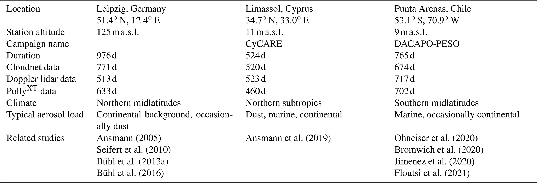
Data coverage for each of the sites is summarized in Table 2. Gaps in the observations were usually caused by periods of short-term deployments at other sites, failure of primary instruments, or power cuts (see also Fig. 1). Coverage with the core instrumentation is generally well above 80 %, the only exception being Doppler lidar and PollyXT at Leipzig.
2.2 Lidar-based aerosol statistics
As a proxy for the aerosol conditions at the three measurement sites, we used vertically resolved observations from the PollyXT lidar system (Althausen et al., 2009; Engelmann et al., 2016). Quantities of interest are the aerosol backscatter coefficient, the extinction coefficient, the particle linear depolarization ratio, and the cloud-relevant concentration of INPs. Their retrieval is explained below.
The basis for the statistical analysis is profiles of particle backscatter coefficient βp at 532 nm wavelength. The profiles are computed with the Klett method (Fernald, 1984) by the PollyNET retrieval whenever atmospheric conditions are suitable (Baars et al., 2016, 2017; Yin and Baars, 2021). The PollyNET retrieval chain also ensures a homogenized analysis of the data from the three different PollyXT instruments which were utilized in the frame of this study (see Fig. 1 and Engelmann et al., 2016; Baars et al., 2016).
Profiles of the particle linear depolarization ratio (hereafter referred to as particle depolarization ratio) are only calculated when the ratio of molecular backscatter coefficient to βp is below a value of 18. Additionally, any particle depolarization ratios larger than 0.7 are masked, as they are indications for noise artifacts in the cross-polarized signal component. All profiles are then filtered with the co-located Cloudnet target classification (see Sect. 2.3) to exclude clouds, especially optically thin ice clouds that are only clearly classified by the cloud radar. Finally, a manual screening excluded fragments of thin liquid clouds, which would otherwise artificially increase βp. For the averages, the optical data of each retrieved profile are binned to vertical intervals of 200 m or 3 K.
The derived average optical properties can be used to estimate aerosol microphysical properties, such as concentrations of ice-nucleating particles (INPs). This is an important step in order to evaluate the datasets of the three sites with respect to contrasts in the potential contribution of aerosol effects on heterogeneous ice-formation efficiency. Conversion from optical properties as observed by lidar to microphysical aerosol properties is based on the parametrizations described by Mamouri and Ansmann (2016). By means of this approach, the lidar-measured aerosol extinction coefficient is converted to the number and surface concentration N500 and S500 of aerosol particles larger than 500 nm in diameter. These quantities are applied in available in situ-based parametrizations for the retrieval of INP concentrations. The prerequisite for the retrieval is a correct aerosol typing, as different types of particles differ by orders of magnitude in their ice-forming efficiency. In order to do so, the average backscatter profile is separated into the categories marine, continental, and mineral dust, based on air mass source (see Appendix B and Radenz et al., 2021) and particle depolarization ratio (one-step POLIPHON; Mamouri and Ansmann, 2017). The average extinction is calculated from the profiles of βp by assuming a typical lidar ratio of 20 sr for marine, 50 sr for continental, and 45 sr for dust aerosol (Müller et al., 2007; Baars et al., 2017; Bohlmann et al., 2018). In a next step, the extinction coefficient is converted to N500 and S500, using sun-photometer-based conversion factors (Mamouri and Ansmann, 2016). Then, the abovementioned INP parametrizations are applied for each aerosol class, such as DeMott et al. (2015) for mineral dust, DeMott et al. (2010) for continental aerosol, and McCluskey et al. (2018b, a) for marine aerosol.
2.3 Cloudnet processing
Synergies between lidar, cloud radar, microwave radiometer, and meteorological data are utilized for the determination of cloud macro- and microphysical properties and as a basis for the stratiform cloud identification scheme. State-of-the-art routines for achieving this synergy are comprised in the Cloudnet retrieval (Illingworth et al., 2007). Cloudnet re-grids the observations to a common resolution (30 s and 31.18 m, determined by the vertical resolution of MIRA-35 with a pulse length of 208 ns) and provides products, such as a target classification and microphysical cloud properties. Re-gridding is a crucial step, as each of the instruments has different temporal and vertical resolution (Table 1). Regular scans of the MIRA-35 cloud radar (hourly) and the Streamline Doppler lidar (twice per hour) are not used within the Cloudnet processing scheme. Profiles of temperature, pressure, and humidity are obtained from the ECMWF's IFS analysis for Punta Arenas and GDAS analysis for Leipzig and Limassol. Liquid water path (LWP) and integrated water vapor (IWV) are retrieved from brightness temperature observations of the microwave radiometer in two frequency bands from 22.24 to 31.4 GHz and 51.0 to 58.0 GHz (seven channels each; Crewell and Löhnert, 2007). The statistical retrieval is based on long-term radiosonde observations (Leipzig and Limassol) and high-resolution reanalysis data (Punta Arenas). Attenuated backscatter of the ceilometer is regularly cross-calibrated with PollyXT using the calibrated attenuated backscatter of PollyNET. Usually, the ceilometer data are used in the synergistic retrieval, as the dataset is more robust and less prone to interruptions. Rare gaps in the observations are filled with the PollyXT attenuated backscatter at 1064 nm.
2.4 Automated cloud selection and characterization
While the Cloudnet algorithm provides a pixel-by-pixel classification of cloud phase and microphysical properties, information on temporal coherence and cloud evolution is not readily available. Hence, an automatic reproducible filtering algorithm for the selection of targeted stratiform, supercooled cloud systems is necessary. Based on the data cube LARDA3 (Bühl et al., 2021), the approach of Bühl et al. (2016) is implemented into an automated selection algorithm.
An example of the Cloudnet processing of measurement data and the application of the cloud selection scheme is shown in Fig. 2. Starting with a profile of the Cloudnet target classification mask (Hogan and O'Connor, 2004), consecutive pixels classified as cloud pixels (liquid droplets, ice, ice and supercooled droplets) are grouped together and defined as features. In case similar types of hydrometeors were observed in matching heights, single features in neighboring time steps are connected to coherent cloud cases. For the analysis, the cloud cases are filtered for shallow stratiform clouds, which are liquid-topped and either have an ice virga or not (rectangles in Fig. 2d). An overview of the microphysical parameters sampled for each cloud case is provided in Table 3. It is assumed that if ice is formed in a liquid layer, it also sediments out of the cloud. This is required, as the signal in the top layer is dominated by return from liquid droplets, and Cloudnet provides no reliable mixed-phase classification there.
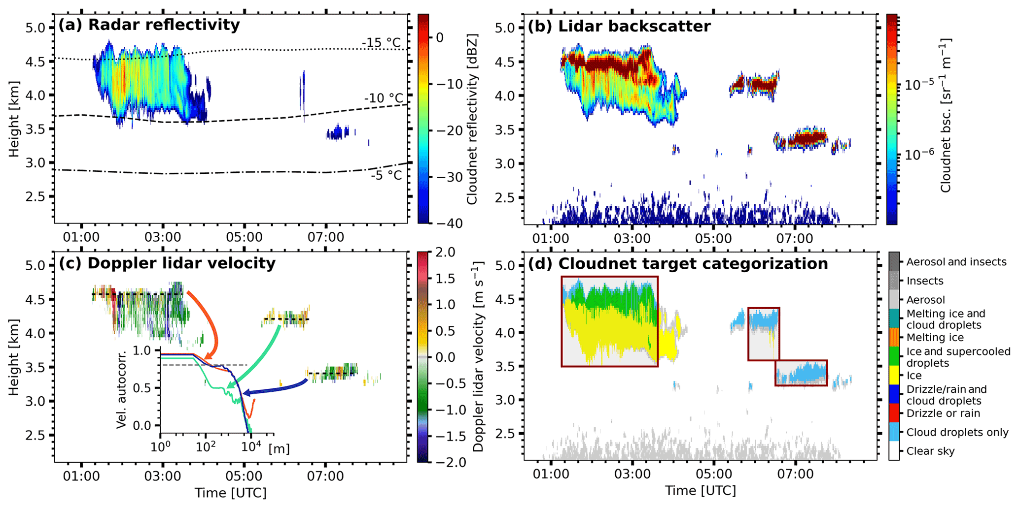
Figure 2Stratiform liquid-topped clouds as observed with LACROS. (a) Cloud radar reflectivity overlaid with the temperature, (b) lidar attenuated backscatter, (c) Doppler lidar vertical velocity, and (d) Cloudnet target categorization (d) on 28 November 2018, 00:20 to 09:00 UTC. The temperature information in (a) is obtained from ECMWF IFS model data. Red rectangles in (d) indicate the automatically detected liquid-topped shallow stratiform clouds. The inset in (c) shows the autocorrelation function of the vertical velocities in the liquid-dominated layer of each cloud. The height of the velocity sampling is indicated with dashed lines. Further details are provided in Sect. 2.5.
Table 3Parameters sampled from the automatically identified cloud cases. A more detailed description of the automated spatiotemporal selection method is provided in Bühl et al. (2016). The IWC and ice extinction are retrieved with the parametrization of Hogan et al. (2006).

To pinpoint the potential effects of aerosol load, thermodynamic and dynamic drivers of ice formation have to be constrained. This is especially important, as the sites are situated in different climate zones. We presume for our study that thin stratiform clouds serve as a natural laboratory, with only a limited number of microphysical processes being possible.
The cloud cases are filtered for a length of more than 20 min and smooth cloud top heights (standard deviation <150 m) to exclude convective clouds. Laboratory studies of Fukuta and Takahashi (1999) and the cloud radar observations by Myagkov et al. (2016) indicate that the average thickness of the liquid-dominated cloud top layer has to be less than 350 m in order to restrict the dataset to the regime of pristine ice formation and avoid strong effects of secondary ice formation. Seeding by ice clouds above is avoided by excluding clouds with ice pixel above the liquid layer. Only cloud cases with top temperatures between −38 and 0 ∘C are considered for the statistics. For the phase occurrence frequency statistics, a cloud is classified as ice-producing if ice pixels were observed 180 m below the liquid-dominated layer within at least 5 % of the duration. On the other hand, cloud cases are classified as liquid-only if ice pixels are observed to sediment out of the liquid-dominated layer less than 5 % of the time. This threshold is simpler than the decision tree used by Bühl et al. (2013a) but provides similar results. The resulting fraction is weighted by the length of the cloud. Similarly to Bühl et al. (2016), the properties of the ice in the virga are taken 180 m below the liquid-dominated cloud top layer to avoid uncertainties in the liquid base estimate and sublimation within the virga. The ice water content (IWC) is derived from the radar reflectivity and the temperature using the Hogan et al. (2006) retrieval. With this automated cloud selection scheme, multi-year datasets can be analyzed using objective criteria while yielding statistics similar to manual cloud selection (e.g., Seifert et al., 2010; Kanitz et al., 2011; Seifert et al., 2015).
2.5 Gravity wave detection
In order to pinpoint effects of aerosol and dynamics on the phase partitioning in the stratiform cloud dataset, an approach is required to assign vertical motion regimes to each cloud case. Here we focus on the temporal structure of vertical velocity, to constrain the dynamics forcing on a cloud. Usually, shallow clouds are characterized by a fully developed turbulence in the liquid-dominated cloud top (Bühl et al., 2019), where the vertical motion is driven by cloud top cooling (e.g., Shao et al., 1997; Fang et al., 2014; Simmel et al., 2015). In the turbulent layer at cloud top, up- and downdrafts alternate at horizontal scales in the order of 100 m or less.
However, orographic gravity waves can trigger vertical motion and associated cloud formation, as well. Microphysical processes in these wave clouds are governed by large-scale dynamics, where vigorous up- and downdrafts may appear stationary. Due to this dynamics, the mixed phase and the ice phase are horizontally separated, with the liquid drops predominantly in the ascending branch and the ice particles in the descending branch (Heymsfield and Miloshevich, 1993; Baker and Lawson, 2006). The properties of the horizontal wind field determine the regions of the up- and downdraft in such orographic clouds. Observing these clouds by stationary ground-based remote sensing might thus not sample the full horizontal extent of the cloud, which causes a misclassification of the cloud case in terms of liquid-only and ice-producing. An illustrative example of such a wave cloud is shown in Appendix A
Also, the flow is highly laminar, as opposed to the confined, fully developed turbulence found in layered mixed-phase clouds. Cloud microphysics in wave conditions cannot directly be compared to layered clouds. For clouds in the heterogeneous freezing regime, Cotton and Field (2002) found that only rapid evaporation freezing once the downdraft commences could explain their observations, where evaporation freezing can be better characterized as inside-out contact freezing of shrinking particles (Durant, 2005). A more recent study by Field et al. (2012) found that condensation and immersion freezing are needed together with deposition and evaporation freezing to explain their aircraft observations of ice formation in wave clouds.
On the other hand, the frequent occurrence of atmospheric gravity waves in a specific region might increase the frequency of thermodynamic conditions that favor the presence of a sustained liquid phase. As Korolev (2007) demonstrates, long-lasting steady updrafts are required in order to make the liquid phase dominate over the ice phase. Probing an observational dataset for the presence of long-lasting updrafts could therefore provide a hint on the role of atmospheric gravity waves in the occurrence of enhanced concentration of supercooled liquid.
Turbulence properties of the liquid layer in the clouds subject to our study can be derived from the vertical velocity observation by Doppler lidar (Bühl et al., 2019). The small size of droplets in the liquid-dominated cloud-top layer and their negligible terminal velocity makes them tracers of air motion. From the Doppler lidar observations, the vertical velocity is sampled at the average height of the center of the layer identified as liquid-containing in the Cloudnet classification. The height of this sampling is indicated by dashed lines in Figs. 2c and A1d. The temporal resolution of the resulting time series is 2 s, i.e., equal to the Doppler lidar raw data. This time series is then used to get insights into the turbulent properties of the cloud-top layer. To separate both regimes in the large dataset, an characteristic parameter is needed. The autocorrelation function was found to be a pragmatic choice for such a parameter.
The autocorrelation function Ψ(τ) for a time series of vertical velocities vt is defined as
with the temporal shift τ and the vertical velocity v at time t. To compare different cloud cases, the autocorrelation function Ψ(τ) is normalized with Ψ(0). The temporal shift τ from the observations is converted into a horizontal shift or autocorrelation length l with the horizontal wind velocity vhor from the model analysis included in the Cloudnet product:
Similarly, the vertical-velocity spectral power density is calculated by a fast Fourier transform of the vertical-velocity time series. High autocorrelation coefficients for large shifts and low power density are indications for wave-driven, low-turbulent flow. The inset in Fig. 2c shows the autocorrelation function for each of the identified cloud cases. All of them are weakly affected by gravity waves, but small-scale turbulence dominates. In contrast, the wave cloud in Fig. A1d shows high autocorrelation coefficients for longer shifts. As a characteristic value of the autocorrelation function, the shift at which the coefficient drops below 0.8 was chosen after visually inspecting the whole dataset. When the ice-formation frequency statistics is investigated for the influence of gravity waves (Sect. 3.2.3), the shift threshold is reduced step by step. As the autocorrelation function is generally decreasing, a lower characteristic value than 0.8 would result in larger shift thresholds. For shifts larger than about 500 m, random fluctuations appear for clouds with a rapid drop in autocorrelation coefficients. Thus, 0.8 is a robust choice for the characteristic value.
In this section, the thermodynamic phase partitioning and quantitative ice mass production in ice-forming shallow cloud layers are presented and compared between all measurement sites under study. First, the average profiles of aerosol optical and microphysical properties are presented. Then, instrumental detection thresholds, boundary layer effects, and gravity wave activity are all analyzed as potential influencing factors on the retrieved ice-formation characteristics.
3.1 Aerosol conditions at Leipzig, Limassol, and Punta Arenas
To provide a general insight into the aerosol conditions at the three sites, the average optical and microphysical aerosol properties as derived from the lidar observations (Sect. 2.2) are shown in Figs. 3 and 4. The impact of aerosol on clouds is controlled more strongly by temperature than geometrical height; hence the averages are also calculated with temperature as a vertical coordinate.
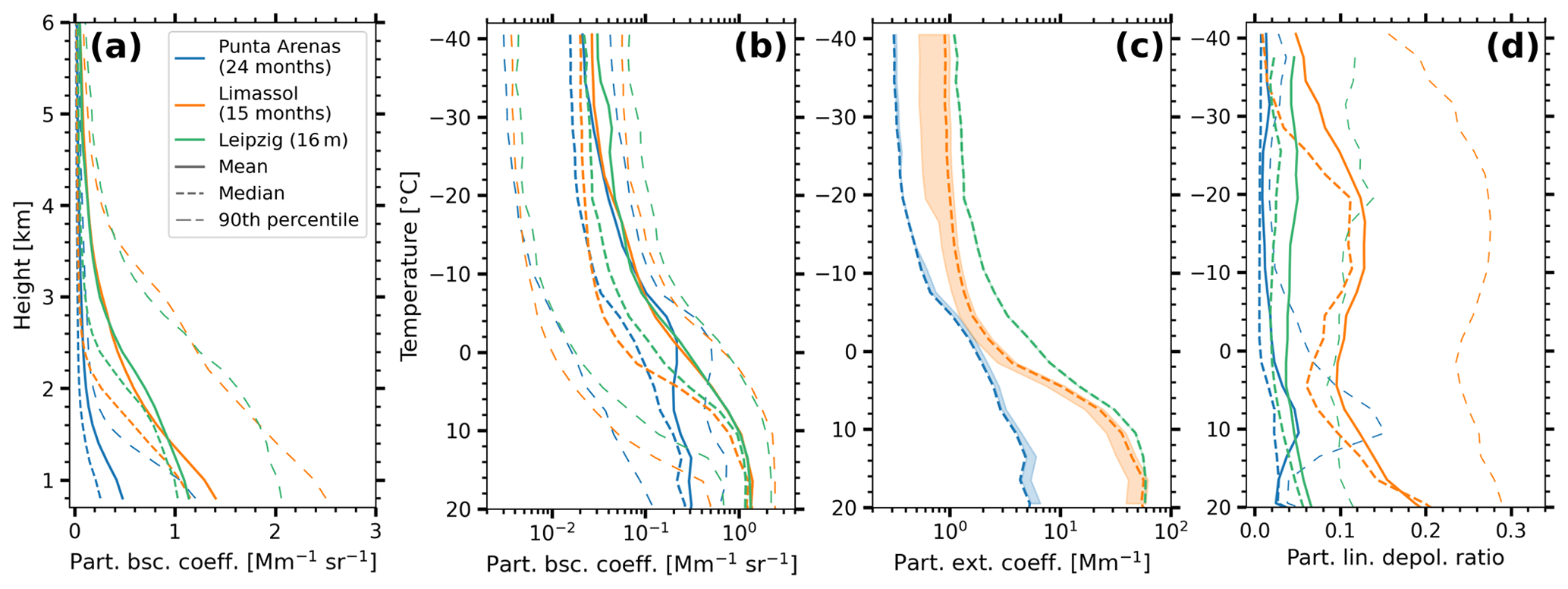
Figure 3Profiles of average aerosol optical properties at 532 nm wavelength derived by the PollyNET retrieval using the Klett method. (a) particle backscatter coefficient over height and (b) temperature for Leipzig, Limassol, and Punta Arenas. (c) Extinction coefficient and (d) particle depolarization ratio for the same locations. For the extinction coefficient, only the median values based on the typical lidar ratio at each site are shown. Variability caused by different aerosol mixtures (see Sect. 3.1.2) is denoted by shading.
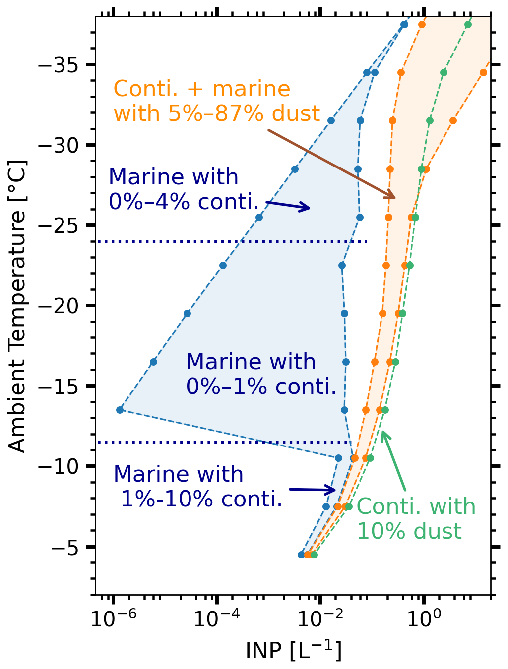
Figure 4Average INP concentrations derived from optical properties for Leipzig (green), Limassol (orange), and Punta Arenas (blue). Shading shows the spread covered by different aerosol compositions, similar to Fig. 3c. Temperature is used as a vertical coordinate. The fraction of continental aerosol is abbreviated “conti.”. The used parametrizations are described in Sect. 2.2.
3.1.1 Optical properties
The average aerosol backscatter coefficient βp at 532 nm and the particle depolarization ratio derived from the PollyXT observations with the Klett method (see Sect. 2.2) are investigated in this section. The evaluation of the air mass sources is covered more quantitatively in the next section and Appendix B.
The central European site of Leipzig is characterized by predominantly continental aerosol mixed with anthropogenic pollution (Baars et al., 2016). Long-range transport of dust may occur periodically, especially during spring and autumn (Ansmann et al., 2003), as well as lofted smoke layers from wildfires (Haarig et al., 2018; Baars et al., 2021). Aerosol optical thickness (AOT) is derived from sun-photometer observations. Mean AOT at 500 nm is 0.198 at TROPOS, Leipzig, between 2014 and 2018. When only the periods with co-located PollyXT observations (used in this study) are considered, the AOT is 0.216. Mean βp at 532 nm drops below only above 4 km height, which corresponds to an extinction coefficient of 1.0 Mm−1, assuming continental aerosol conditions and a corresponding lidar ratio of 50 sr.
Limassol is characterized by a distinct dry season with no precipitation and very few clouds during the summer. Generally, Limassol is frequently affected by aerosol transport from Africa, the Middle East, and Europe, with aerosol characteristics including dust (mineral and soil), marine (organics and sea salt), and anthropogenic pollution as well as mixtures of these (Nisantzi et al., 2015). Mean AOT at 500 nm is 0.176 during the whole observational period and 0.165 during the “cloudy season” from October to May. In the following, the non-cloud season from June to September is excluded from the statistics. The profile of mean backscatter is similar to the one at Leipzig within a factor of 1.5, whereas the median generally is higher at Leipzig.
The aerosol load at Punta Arenas can be separated into two distinct layers, with an aerosol-rich boundary layer and pristine conditions aloft. The free troposphere is dominated by marine aerosol from the Southern Ocean and was reported to show no changes compared to pre-industrial conditions (Hamilton et al., 2014). Nevertheless, events of aerosol long-range transport also occur occasionally (Foth et al., 2019; Floutsi et al., 2021). The boundary layer is laden with a mixture of marine and continental aerosol, as Punta Arenas is located 230 km inland from the Pacific coast. Mean AOT at 500 nm is 0.055 during the whole campaign but drops to 0.047 when excluding the period of long-range wildfire smoke transport in early 2020 (Ohneiser et al., 2020). Average boundary layer height is around 1.5 km (Foth et al., 2019) with negligible βp above 2.0 km height (90 % percentile of βp at 532 nm dropping below ). Comparing the backscatter at Punta Arenas and Limassol, the 90 % percentile at Punta Arenas is more than 30 % below the mean of Limassol and Leipzig at similar heights above ground. Both European sites show quite some variability, as well, with the 90 % percentile βp twice as large as the mean.
At temperatures above 5 ∘C, βp shows the strongest difference between the three sites (Fig. 3b), also explaining the larger AOT at Limassol and Leipzig. Between 0 and , the mean βp at Limassol and Punta Arenas is almost equal. This counterintuitive behavior can be explained by different temperature regimes. The isotherm at Punta Arenas varies between 1.1 and 3.3 km height, whereas at Limassol it varies between 3.0 and 4.8 km height and at Leipzig between 2.1 and 4.8 km. At Punta Arenas, corresponding to the height of 2.0 km, only very low values of βp are observed at heights below a temperature of . The pronounced decrease of backscatter at Leipzig and Limassol is observed at slightly higher temperatures, which agrees with the, on average, higher boundary layer temperature there. Assuming typical lidar ratios of 50 (continental), 45 (dust), and 20 sr (marine) at Leipzig, Limassol, and Punta Arenas, respectively, typical aerosol extinction coefficients can be estimated from the median βp profile (Sect. 2.2). As shown in Fig. 3c, the extinction coefficients at Punta Arenas are a factor 2–3 lower than over Limassol for temperatures below . This difference decreases to a factor of 1.5 for slightly supercooled conditions of above . Comparing Punta Arenas and Leipzig, the extinction is a factor of 3–4 higher at the latter site for all temperatures below freezing. These optical properties serve as a proxy for the background reservoir of aerosol particles that could act as cloud condensation nuclei and ice-nucleating particles in the free troposphere.
The particle depolarization ratio provides hints on the aerosol particle types (Fig. 3d). At Leipzig, the depolarization ratio is approximately 0.05 at all temperatures, typical for a continental aerosol with a slight contribution of mineral dust. The depolarization ratio at Limassol is bimodal, with one peak above 20 ∘C, a second one at , and a minimum at 4 ∘C. The first peak can be ascribed to mineral dust in the boundary layer and originating from local sources. The second one at is caused by long-range transport of mineral dust. At Punta Arenas, a maximum at is caused by occasional events of dried sea salt aerosol at the top of the atmospheric boundary layer (Haarig et al., 2017; Bohlmann et al., 2018). Going to lower temperatures, the depolarization ratio has a minimum of 0.01 at and a slight increase afterwards.
3.1.2 Contrasts in INP concentrations
An important aspect for the discussion of microphysical contrasts in clouds over the three sites is how the differences in aerosol optical profiles are linked to contrasts in the INP load. An estimate of average INP concentrations covering the whole troposphere can be derived with the parametrizations described in Sect. 2.2. The decision for the aerosol typing required in the INP retrieval is based on the particle depolarization ratio and air mass source estimates. The air mass source methodology is based on Radenz et al. (2021) and shown in Appendix B.
At Punta Arenas marine sources are by far the most frequent, contributing 90 % to the residence time throughout the troposphere and peaking 95 % at 2.7 km height. Only below 2.0 km height (or above ) do local terrestrial sources make up to 10 % of the air mass. Above 5 km height (below ) sparsely vegetated areas in Australia contribute up to 4 % to the air mass source. Mean particle depolarization ratios below 0.02 in the free troposphere exclude frequent presence of mineral dust (Fig. 3d). Contrarily, at Limassol, air masses with a marine source contribute 50 % to 80 % to the mixture. But these air masses are not pristine marine, as the eastern Mediterranean is enclosed by strongly populated landmasses. Below 5 km height (above ), continental Europe is the second strongest source, responsible for up to 45 % at 0.5 km height. In the upper troposphere, barren ground from the Sahara is the strongest terrestrial source, with contributions around 15 %. POLIPHON (see Sect. 2.2) shows a peak at with mean dust fractions of 0.3 (90 % percentile 0.87). Hence, the backscatter is divided into dust and non-dust according to the dust fraction. The non-dust portion is then split up into continental and marine, with 40 % contribution of the continent above and 20 % below. The aerosol mixture at Leipzig is dominated by continental aerosol, with an average dust fraction of 0.1.
The derived INP concentrations are depicted in Fig. 4. Note that the INP concentration at a certain atmospheric temperature (as a proxy for height) is shown based on the optical properties, aerosol types, and the parametrization, not a freezing spectrum obtained from sampling a single air parcel and varying temperature.
At temperatures above , average INP concentrations between and can be expected at all three locations. With decreasing temperatures, the concentration increases to 0.1–1 L−1 at at the northern hemispheric sites of Leipzig and Limassol. A strong increase of ice-nucleating efficiency with decreasing temperature is counterbalanced by a decreasing aerosol concentration at lower temperatures, which are tied to greater heights. INP concentrations at Punta Arenas are strongly controlled by the fraction of continental aerosol in the free troposphere. Continental sources can contribute up to 1 % between −11 and and up to 4 % at lower temperatures. When only pristine marine aerosol is present, the INP concentration can expected to be 3–4 orders of magnitude lower than at the two other sites. Equally low concentrations of INPs were also found by McFarquhar et al. (2021) in the remote Southern Ocean, south of Australia. As soon as very small fractions of continental aerosol are present, the INP concentration increases significantly. However, even if a few percent of continental aerosol are assumed, throughout the heterogeneous freezing regime, INP concentrations remain a factor of 2–6 lower at Punta Arenas, compared to Leipzig and Limassol. Due to the absence of suitable remote-sensing or in situ measurements, the actual contribution of continental aerosol to the free tropospheric aerosol load over Punta Arenas can to date not be obtained. The range given in Fig. 4 is thus a solid estimate of the expectable range of possible INP concentrations. At temperatures above , which refers to a height range that is frequently within the boundary layer, INP concentrations at Punta Arenas are high and within an order of magnitude of the concentrations at Leipzig and Limassol at the same temperature. Concentrations that are equally high as retrieved from the remote-sensing observations above were also found in situ at the upwind hilltop station on Cerro Mirador at an altitude of (Gong et al., 2021).
3.2 Mixed-phase stratiform cloud properties
The automated stratiform cloud selection algorithm introduced in Sect. 2.4 is applied to the Cloudnet datasets of all three locations. An overview over identified clouds and temperature-resolved phase occurrence frequency is provided in Sect. 3.2.1. Afterwards, it is shown how boundary layer aerosol load (Sect. 3.2.2) and gravity waves affect the phase occurrence (Sect. 3.2.3). In Sect. 3.2.4 contrasts of ice content in the virga are briefly discussed.
3.2.1 Phase occurrence frequency and detection thresholds
Figure 5 shows all the cloud cases that fulfill the selection criteria introduced in Sect. 2.4. The time share of ice virga sedimenting out of the liquid-dominated top is given by the fraction of profiles for which ice was classified below the liquid layer. Values range from 0 (no ice virga observed at all) to 1 (ice virga observed all the time). At all three locations, the fraction of profiles (i.e., fraction of time) in which a virga originated from the liquid layer increases with decreasing temperature. Similarly, the ice-to-liquid content ratio (Bühl et al., 2016) increases for lower temperatures. Liquid-only clouds (fraction of profiles where no ice was produced from the liquid layer) were observed at Leipzig and Limassol down to , whereas at Punta Arenas, such clouds were observed even at temperatures as low as .
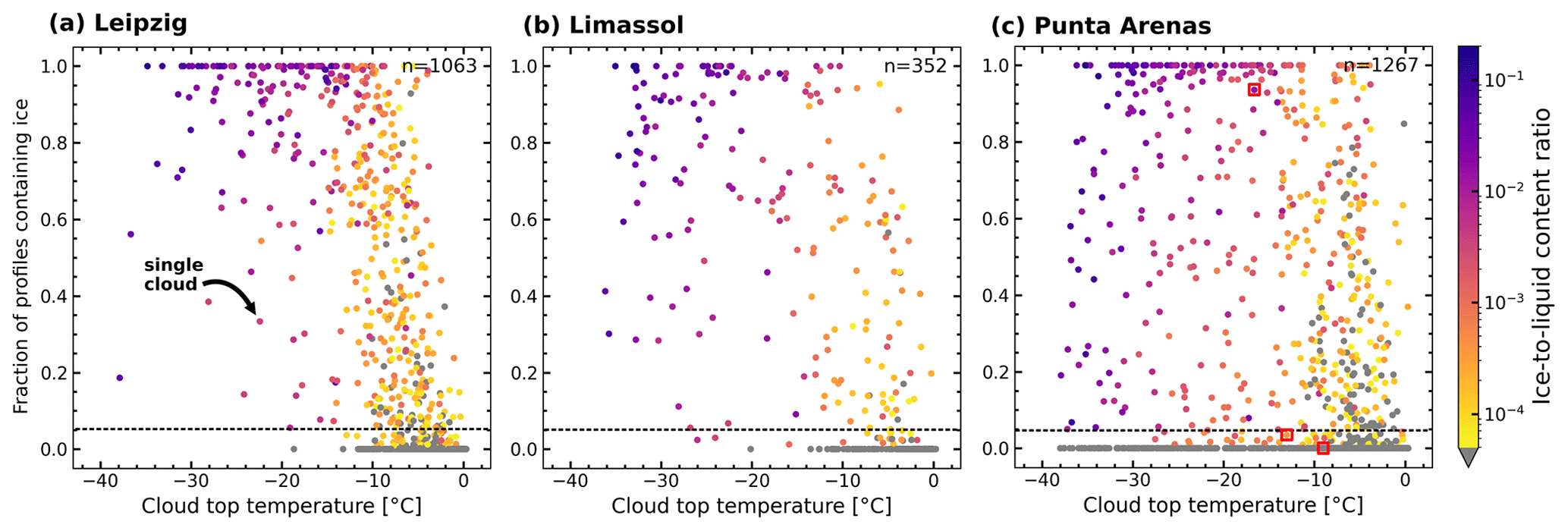
Figure 5All stratiform clouds identified by the automated selection algorithm for (a) Leipzig, (b) Limassol, and (c) Punta Arenas by their cloud top temperature and the fraction of profiles, where ice is observed below the liquid-dominated cloud top. The 0.05 threshold for the classification is marked by a dashed line. The color gives the median ice-to-liquid content ratio. n gives the number of cloud cases in each dataset. Red squares in (c) denote the clouds also shown in Fig. 2.
First, the temperature-resolved fraction of occurrence of ice-forming clouds is depicted in Fig. 6. For the phase occurrence frequency, a cloud is classified as ice-producing, if an ice virga was observed during at least 5 % of the duration of a cloud case (Sect. 2.4). Comparing the frequency of ice-containing clouds at different locations provides insights into differences of primary ice formation (Choi et al., 2010; Kanitz et al., 2011; Seifert et al., 2015; Tan et al., 2014; Zhang et al., 2018). Generally, clouds contain ice more frequently for decreasing temperature (Fig. 6, solid lines). While at Leipzig and Limassol nearly all clouds with CTTs below contained ice, at Punta Arenas a fraction of 0.4±0.1 of shallow stratiform clouds at these temperatures were classified as liquid-only. This behavior is discussed further in Sect. 3.2.3.
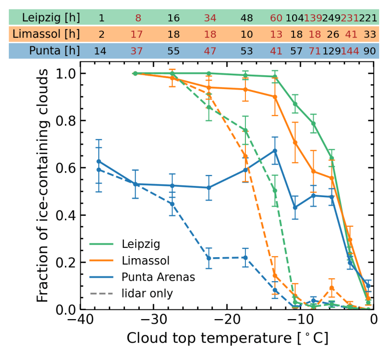
Figure 6Fraction of ice-containing clouds over temperature for Leipzig, Limassol, and Punta Arenas. Total duration of the clouds in each bin is given by the numbers above in hours. Dashed curves mark the occurrence frequency when using a lidar detection threshold of 12 Mm−1.
Compared to prior lidar-based studies (e.g., Kanitz et al., 2011; Choi et al., 2010; Seifert et al., 2010), the fraction of ice-containing clouds in the synergistic dataset is higher at temperatures above . At these temperatures, the amounts of ice produced and, hence, the radar reflectivity and optical extinction are usually very low and stay undetected for lidar (Bühl et al., 2013a) and spaceborne radars (Bühl et al., 2016). To quantify a lidar detection threshold in terms of optical extinction, the reflectivity-to-IWC and the reflectivity-to-extinction relationships by Hogan et al. (2006) are used. The only additional information needed for both parametrizations is the ambient temperature. Using these relationships, the response of the occurrence statistics to arbitrary extinction detection thresholds can be tested. As shown in Fig. 6 (dashed lines), for the lidar data used in the Cloudnet classification, an extinction threshold of 12 Mm−1 had to be applied in order to best match the lidar-only statistics from Punta Arenas and Leipzig presented by Kanitz et al. (2011).
3.2.2 Effect of boundary layer aerosol load on phase occurrence
As discussed in Sect. 3.1, the aerosol load at Punta Arenas is confined to the lowermost 2 km, and the aerosol load at temperatures above is similar to Limassol. To check for possible impact of this boundary layer aerosol on the ice-formation efficiency, the basic temperature-resolved phase occurrence frequency (Fig. 6) is split into two subsets, one containing cloud cases with bases below 2 km height and one with cloud cases having bases above that threshold, in the following denoted as coupled and uncoupled clouds, respectively. The resulting ice-formation frequency is shown in Fig. 7. At any height, temperatures vary by more than 11 ∘C (10 % to 90 % percentile), providing ample coverage for the height threshold. Generally, coupled clouds show higher fractions of ice (absolute difference increases by 0.3 at all locations at ). The temperature-resolved phase occurrence frequency for the coupled clouds shows rapid increase in fraction of ice-containing clouds, reaching 1.0 at temperatures of only . The absolute difference between the fractions is less than 0.20, with the lowest fractions still being observed at Punta Arenas. Below , almost no clouds were observed at such low heights, especially at Limassol; hence no meaningful comparison can be done in this temperature interval.
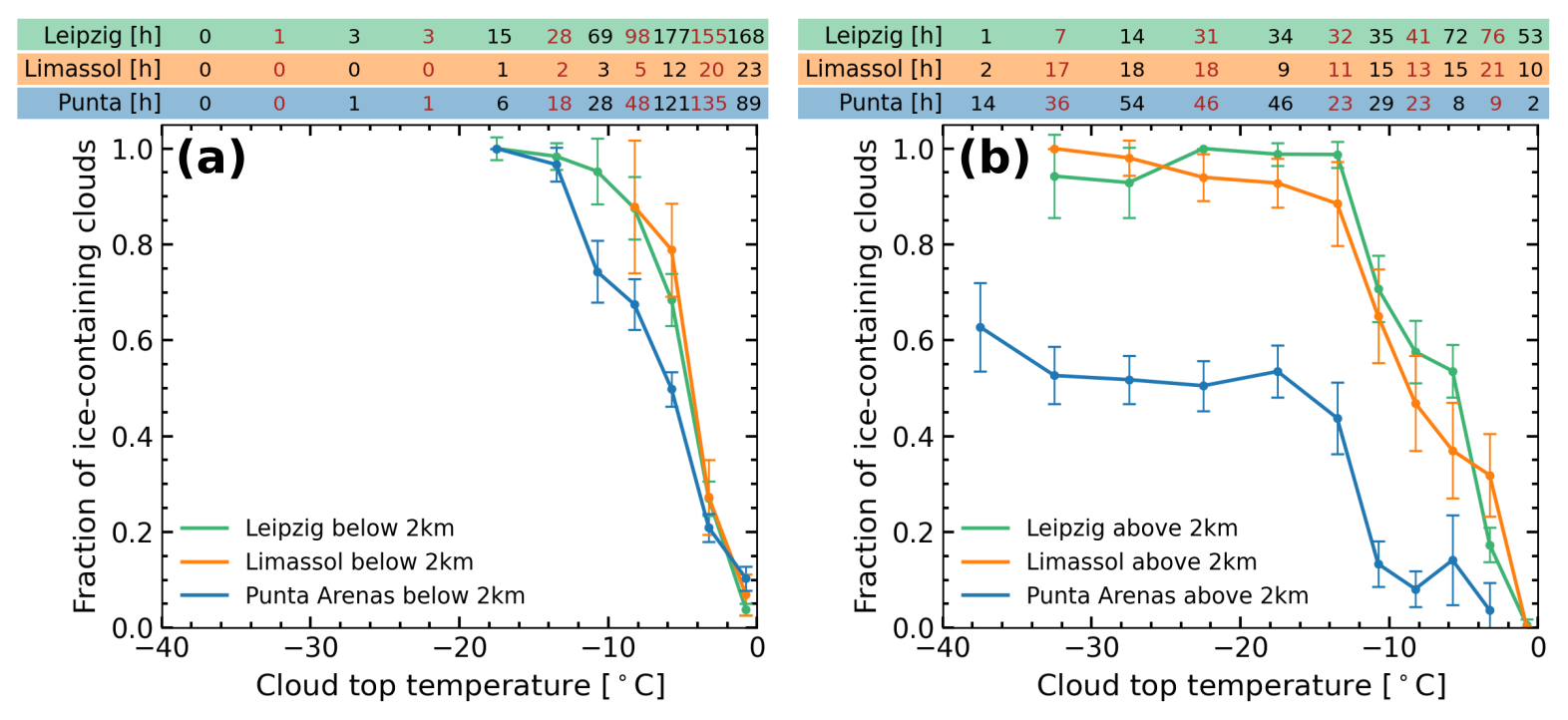
Figure 7Fraction of ice-containing clouds over temperature for Leipzig, Limassol, and Punta Arenas, (a) below 2 km and (b) above 2 km. Total duration of the clouds in each bin is given by the numbers above in hours.
Considering only uncoupled clouds (cloud base above 2 km height; Fig. 7b), stronger contrasts become evident. The wave clouds discussed in the following section are still included and impact the frequency at temperatures below at Punta Arenas. The frequencies of ice-forming clouds are similar at Leipzig and Limassol but 0.15 to 0.5 at lower at Punta Arenas. Comparing the coupled and uncoupled state at Leipzig and Limassol, ice formation is more frequent in the coupled case by 0.15 between −5 and .
3.2.3 Gravity wave influence on phase occurrence at low temperatures
The lower frequency of ice-containing cloud layers at temperatures below over Punta Arenas is a prominent feature of both the lidar–radar and the lidar-only-equivalent datasets shown in Fig. 6. The associated high abundance of supercooled liquid water is frequently reported as a general phenomenon of stratiform clouds in the Southern Hemisphere midlatitudes and higher latitudes. Within this subsection, the reasons for the found behavior over Punta Arenas will be elaborated in more detail.
Frequently, the stratiform liquid-only cloud layers observed over Punta Arenas at temperatures below are embedded in orographic gravity waves. Following the wave detection methodology introduced in Sect. 2.5, Fig. 8 shows the autocorrelation and power spectra of the Doppler lidar vertical velocity for clouds classified as liquid-only over Leipzig, Limassol, and Punta Arenas, respectively. These supercooled liquid-only clouds at Punta Arenas show high autocorrelation coefficients at long shifts (Fig. 8c1), whereas liquid-only clouds with similar characteristics are absent at Limassol (Fig. 8b1) and Leipzig (Fig. 8a1). In terms of spectral power density (Fig. 8c2), the strongly supercooled clouds at Punta Arenas show only low turbulence.
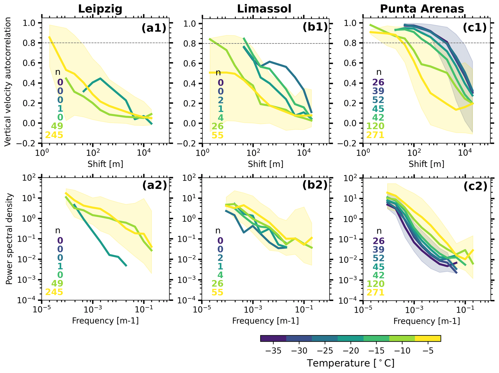
Figure 8Vertical-velocity autocorrelation function (a1, b1, and c1) and power density (a2, b2, and c2) of the Doppler lidar vertical velocities for cloud cases classified as liquid-only. The columns are (a) Leipzig, (b) Limassol, and (c) Punta Arenas. The curves are binned to CTT intervals of 5 K with color indicating the CTT. The number of clouds for each temperature interval is given as numbers in the respective panel. Shading denotes the 10 %–90 % percentile range for the −5 and bin.
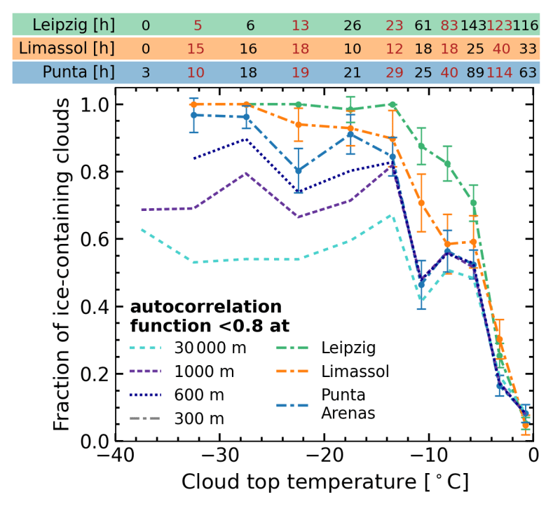
Figure 9Fraction of ice-containing clouds over temperature for Leipzig, Limassol, and Punta Arenas. Dashed–dotted lines show the fractions for Leipzig, Limassol, and Punta Arenas with an autocorrelation coefficient smaller than 0.8 for a horizontal shift of 300 m. The fractions for cloud cases with longer autocorrelation are only shown for Punta Arenas. The total duration of the clouds in each bin is given by the numbers above in hours.
In a next step, the autocorrelation is used to filter the dataset for clouds affected by gravity waves. As described in Sect. 2.5, the length at which the autocorrelation coefficient drops below 0.8 is used as a characteristic value. Decreasing the threshold value for this characteristic length will remove gravity-wave-influenced clouds from the dataset. For large values of the length threshold, e.g., larger than 1000 m, only clouds that are strongly forced by gravity waves will be removed, whereas going to shorter thresholds (<500 m) will also remove weakly gravity-wave-influenced clouds. Figure 9 shows an increase in the fraction of ice-containing clouds below with decreasing correlation-length thresholds from 30 000 to 300 m. At Punta Arenas, the fraction of ice-containing clouds increases from 0.5 to 0.85. In the temperature interval between −15 and , the fraction is 0.05 to 0.1 lower at Punta Arenas compared to Leipzig and Limassol. Hence, clouds with fully developed turbulence show similar ice-formation frequencies, independent of the location, with indications for a still slightly reduced ice-formation efficiency over Punta Arenas.
3.2.4 Comparison of radar reflectivity factor of the ice virga
Prior studies of Zhang et al. (2018) identified a strong contrast in radar reflectivity factor between the different 30∘ latitude bands of the globe, with the Southern Hemisphere midlatitudes (30–60∘ S) showing the lowest mean reflectivity of all regions. They concluded that this difference in reflectivity factor is associated with a respective difference in ice crystal mass and number concentration. In the following we provide a similar representation of regional contrasts of ice-virga reflectivity from ground-based perspective that is based on a single radar instrument. As described in Sect. 2.4, the amount of ice formed in the mixed-phase layer is measured at six height bins (180 m) below the base of the liquid-dominated cloud top and hence at the top of the virga (Bühl et al., 2016). Figure 10a shows the cloud top temperature-resolved statistics of reflectivity for the three stations, which is based on the full cloud dataset, including the wave-influenced clouds (as these are also included in the study by Zhang et al., 2018). From −28 to and again above , Punta Arenas shows the lowest reflectivity and Limassol the highest. For most temperatures, Punta Arenas is 5–8 dB below the northern hemispheric stations; the only exception is the interval between −4 and , where the reflectivity for Punta Arenas and Leipzig is almost equal. At temperatures below , Limassol and Punta Arenas show equal reflectivity, with values at Leipzig being slightly higher.
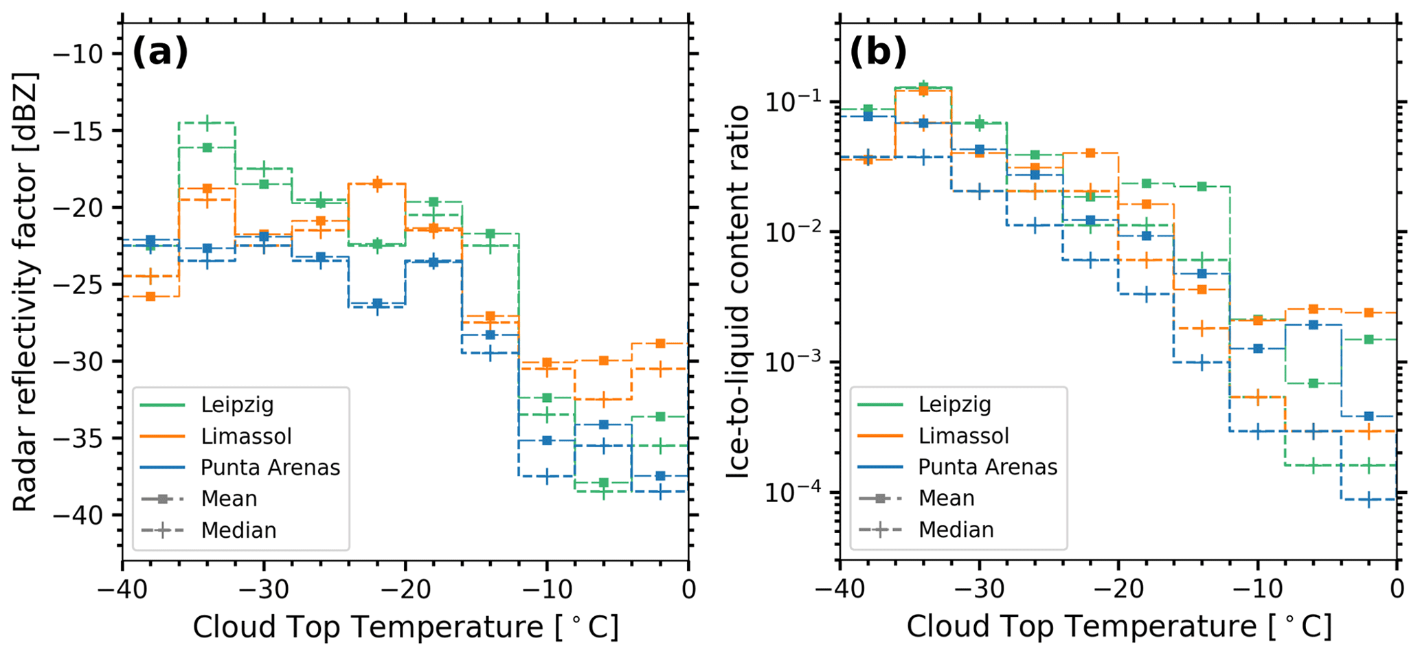
Figure 10Amount of ice observed in the virga, (a) radar reflectivity factor observed at the top of the virga (180 m below the liquid-dominated layer base) and (b) ice-to-liquid content ratio binned by CTT. Temperature bins of 4 ∘C.
We further investigated the properties of the ice-forming liquid-dominated cloud top layers and found that cloud thickness agrees within 40 m above . The ice-to-liquid content ratio (Fig. 10b) is smaller at Punta Arenas than at the northern hemispheric locations, especially (factor 3) between −24 and but also above . Hence, in these temperature regimes, the liquid phase is less efficiently converted into ice in stratiform clouds above Punta Arenas.
In the previous section, a comprehensive overview of the aerosol conditions and stratiform cloud properties at the strongly contrasting sites of Leipzig, Limassol, and Punta Arenas was presented. Several aerosol-, temperature-, surface-coupling-, and dynamics-related differences have been identified and will be discussed in the following.
The analysis of the profiles of aerosol optical properties obtained from the PollyXT lidar observations reveals almost similar aerosol load at Punta Arenas and Limassol between 0 and . Leipzig shows a higher aerosol load in this temperature interval. For lower temperatures, the lowest average extinction was observed at Punta Arenas. Low values of particle depolarization ratio indicate that non-spherical particles, such as mineral dust, are completely absent at Punta Arenas below . The absence of continental aerosol species in the free troposphere is also consistent with the Southern Ocean, south of Australia (e.g., Alexander and Protat, 2019). Additionally, Uetake et al. (2020) showed for this region that INPs are related to sea spray emissions. Together with an air mass source estimate, the average profiles of optical parameters were used as an input for INP parametrizations for a first estimate of long-term averages of INP concentrations. The lidar-based estimate of average INP concentrations identifies the strongest differences in INP concentrations between −12 and . However, it is still subject to discussion as to which fraction of marine particles is transported from the boundary layer to the free troposphere. This insufficient knowledge propagates further into uncertainties in the fraction of continental aerosol, which leads to considerable uncertainties in the estimated concentrations of INPs. Bourgeois et al. (2018) argue that due to efficient removal processes, marine particles predominantly remain in the boundary layer (globally 80 % of their AOT). Murphy et al. (2019) argue in a similar direction, especially when sea salt is regarded a tracer of marine origin.
Opposed to prior lidar-only studies (e.g., Kanitz et al., 2011; Alexander and Protat, 2018), more than half of the clouds observed at at the three sites were found to contain ice. This is in line with the lidar detection threshold introduced by Bühl et al. (2013a) but extending their results to Limassol and Punta Arenas. This result has significance for lidar-only or ceilometer datasets that are currently used for validation of climate models (e.g., Kuma et al., 2020). The occurrence of ice at these relatively warm temperatures is also in line with airborne in situ observations over the Southern Ocean (Huang et al., 2017; D'Alessandro et al., 2019).
Ice formation at slightly supercooled conditions above was found to be equally frequent, suggesting the presence of equally efficient INPs at all sites. At Punta Arenas, such temperatures usually occur within the boundary layer, where presumably INPs of biological origin are present (Gong et al., 2021). Similarly high fractions were also observed for Arctic boundary layer clouds during summer and autumn (Achtert et al., 2020). Griesche et al. (2021) also found that surface coupling increased the frequency of ice formation in boundary layer clouds observed during Arctic summer.
The liquid-only clouds at Punta Arenas found below are identified to be predominantly wave clouds forced by orography, likely in an early period of their life cycle. In this kind of cloud, the liquid-dominated mixed phase is separated horizontally from the ice virga, due to the rapid flow and weak turbulence (Heymsfield and Miloshevich, 1993). When sampled by stationary observations, only parts of the clouds are covered, and the phase occurrence frequency is biased. Using Doppler lidar vertical velocity observations, clouds driven by orographic wave dynamics can be identified based on their autocorrelation function, as presented in Sect. 3.2.3. At temperatures below , approximately one-third of the cloud layers observed at Punta Arenas were influenced by gravity waves. Similar frequencies of occurrence of non-turbulent liquid layers were also found at Utqiaġvik (Alaska) and McMurdo (Antarctica), deriving stability criteria from radiosoundings (Silber et al., 2020).
In a final step, the separation techniques for coupling and orographic waves can be combined to assess contrasts in ice frequency for free tropospheric and fully turbulent clouds. The resulting occurrence frequency is shown in Fig. 11. The fraction of ice-containing clouds at temperatures below is above 0.85 at all three sites. However, in comparison to Leipzig and Limassol, the fraction of ice-forming clouds with CTT between −25 and remains 0.1 lower at Punta Arenas. Mineral dust is known to be an efficient INP at these temperatures (Kanji et al., 2017) but was not observed at the respective temperatures at Punta Arenas (Fig. 3). This difference in the non-wave cloud phase occurrence is also in agreement with satellite-based studies of Villanueva et al. (2020), who also attributed latitudinal differences in the ice occurrence to associated differences in the dust load. Figure 11 also depicts the low frequency of ice formation in free tropospheric fully turbulent clouds at temperatures above . With less coupling to the near-surface aerosol reservoir, ice formation is strongly suppressed compared to Leipzig and Limassol.
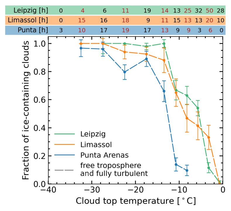
Figure 11Fraction of ice-containing clouds over temperature for Leipzig, Limassol, and Punta Arenas when considering only fully turbulent clouds with an autocorrelation coefficient smaller than 0.8 for a horizontal shift of 300 m (see Fig. 7) and cloud bases in the free troposphere above 2 km height (see Fig. 9).
The ice mass formed by stratiform liquid layers is lowest at Punta Arenas, as was found by investigating the radar reflectivity factor in the ice virga as a proxy. Especially between −28 and , the observed radar reflectivity factor is up to 7 dB lower, compared to both sites in the Northern Hemisphere. This result is consistent with estimates from spaceborne sensors covering the full Southern Ocean (Zhang et al., 2018). In contrast, Arctic mixed-phase clouds were found to respond with lower IWC to increased loads of anthropogenic pollution (Norgren et al., 2018). As for the lower frequency of ice formation discussed above, the difference in ice mass coincides with a lack of dust INPs at these temperatures. Slight differences in IWC or radar reflectivity, respectively, might be explained by a slower mass growth rate, caused by a smaller vapor diffusion coefficient at higher ambient pressure (Hall and Pruppacher, 1976). When temperature and particle size are considered similarly, the stratiform clouds subject to this study experience 10 % to 20 % larger growth rates at Leipzig and Limassol than at Punta Arenas. Hence, the difference of a factor 3–6 larger ice mass cannot be explained solely by this effect alone.
Frequent occurrences of ice-forming clouds above were found, which were not covered by studies based on spaceborne active remote sensing. Similar to their colder counterparts, they show a lower ice amount in the virga above Punta Arenas but with a smaller difference compared to the sites in the Northern Hemisphere. With an average reflectivity of −36 dBZ, they are usually well below the detection limit of the CloudSat satellite in the A-Train constellation (Bühl et al., 2013a, 2016). Occurrence of such clouds in other parts of the Southern Ocean cannot be ruled out. A misclassification of supercooled drizzle clouds as ice-containing is unlikely, as they exceed −30 dBZ neither at cloud top, nor in the virga. From previous studies it is known that the onset of drizzle formation is usually associated with higher reflectivities, either above approximately −20 dBZ (Liu et al., 2008; Acquistapace et al., 2019) or at least above −30 dBZ (Wu et al., 2020).
This study investigated contrasts in aerosol–cloud interactions in shallow supercooled stratiform clouds observed with the ground-based remote-sensing supersite LACROS at Leipzig, Limassol, and Punta Arenas.
Sampling the profiles of optical properties with temperature as a vertical coordinate revealed aerosol load at temperatures between −15 and 0 ∘C being within a factor of 2 at Punta Arenas and Limassol. This finding is related to the cold and (compared to the free troposphere) aerosol-laden boundary layer at Punta Arenas. At lower temperatures, the lowest βp and extinction were observed over Punta Arenas, the highest over Leipzig. The very low particle depolarization ratio at Punta Arenas between −25 and suggests the absence of mineral dust in a temperature regime, where dust is known to be an efficient INP. An estimate of INP concentrations at the respective temperatures based on the optical properties reveals differences of 1–4 orders of magnitude between Punta Arenas and the two northern hemispheric sites. In absence of abundant INPs from marine sources, the contribution of terrestrial sources causes strong variability.
The phase occurrence frequencies showed a higher fraction of ice-containing clouds at weakly supercooling temperatures of above compared to prior lidar-only studies. A cloud radar with a sensitivity better than −40 dBZ is needed to sufficiently characterize low ice water contents in the virga formed by shallow stratiform clouds in this temperature regime. Coupling to the boundary layer increases the frequency of ice formation at slightly supercooling temperatures at all sites. The strongest contrasts in the ice-formation frequency between free tropospheric and surface-coupled conditions were found for Punta Arenas. This finding is in compliance to the found contrasts in the INP profiles at the three sites and further indicates that the free tropospheric INP reservoir over the Southern Ocean is limited.
Frequent liquid-only layers below at Punta Arenas were found to be associated with orographic gravity waves, causing two implications: (1) potential phase misclassification by stationary observers due to horizontal separation of ice and liquid phase and (2) sustained liquid water in updrafts because the associated vertical velocities allow for supersaturation over water; the newly developed Doppler lidar autocorrelation approach helps to address “[…] the difficulty in characterizing gravity waves from existing single-site measurements […]” as posed by Silber et al. (2020). Ice mass in the virga and the ice-to-liquid content ratio were found to be lowest at Punta Arenas, especially at temperatures where dust serves as an efficient INP at the northern hemispheric sites.
From the results of this study, two issues for further investigations arise: firstly, the importance of terrestrial sources of INPs in the Southern Ocean. Observations of free tropospheric aerosols upwind and downwind of major landmasses are required to quantify the terrestrial emission and identify regions where the emitted INPs impact cloud microphysics the strongest. Secondly, how important are gravity waves in the formation of clouds in other regions of the Southern Ocean? How frequently do gravity waves occur above the open ocean, which covers the vast majority of the Earth's surface between 30 and 70∘S? Such measurements are required in order to further constrain the role of INPs in the evident excess of liquid water in clouds of the southern hemispheric midlatitudes.
Figure A1 shows a typical wave cloud at Punta Arenas. Updrafts in stationary or slowly propagating waves can sustain liquid layers without showing signatures of sedimenting ice crystals to the fixed observer. The ice phase is only visible downwind as soon as the droplets have evaporated. Such a wave cloud was observed at Punta Arenas on 27 September 2019. A mid-tropospheric long-wave ridge caused a strong, zonal westerly flow at Punta Arenas. Velocity of the horizontal wind exceeded 25 m s−1 at 4000 m height. Layered clouds developed within the orographic gravity waves triggered by this flow. One of the cloud layers with a CTT between −34 and is depicted in Fig. A1. It illustrates how the liquid and ice phase are horizontally separated. Embedded in a slowly propagating gravity wave, the cloud was advected over the site, and the full life cycle could be observed. Based on the Doppler lidar vertical velocity (Fig. A1d), the updraft was present until 05:32 UTC. Afterwards, downward motion with increasing velocity set in. Only after the liquid droplets evaporated at 06:17 UTC can the ice particles be clearly identified in the remote-sensing observations (Fig. A1b, c).
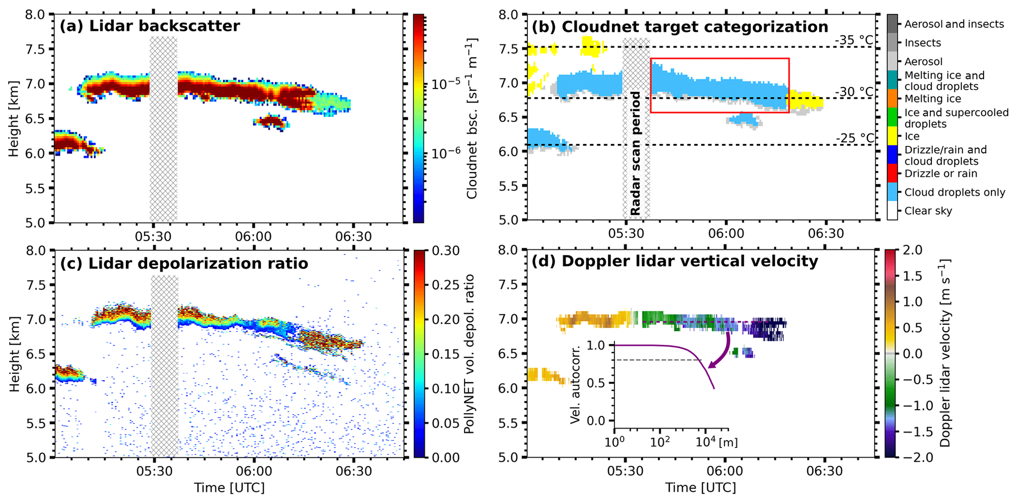
Figure A1Wave cloud observed at Punta Arenas on 27 September 2019, 05:00–06:45 UTC. (a) Lidar attenuated backscatter, (b) Cloudnet target categorization, (c) lidar volume linear depolarization ratio, and (d) Doppler lidar vertical velocity. The temperature information in (b) is obtained from ECMWF IFS model data. The red rectangle in (d) indicates the automatically detected liquid-topped shallow stratiform cloud. The inset in (d) shows the autocorrelation function of the vertical velocities in the liquid-dominated layer. The height of the velocity sampling is indicated with a dashed line.
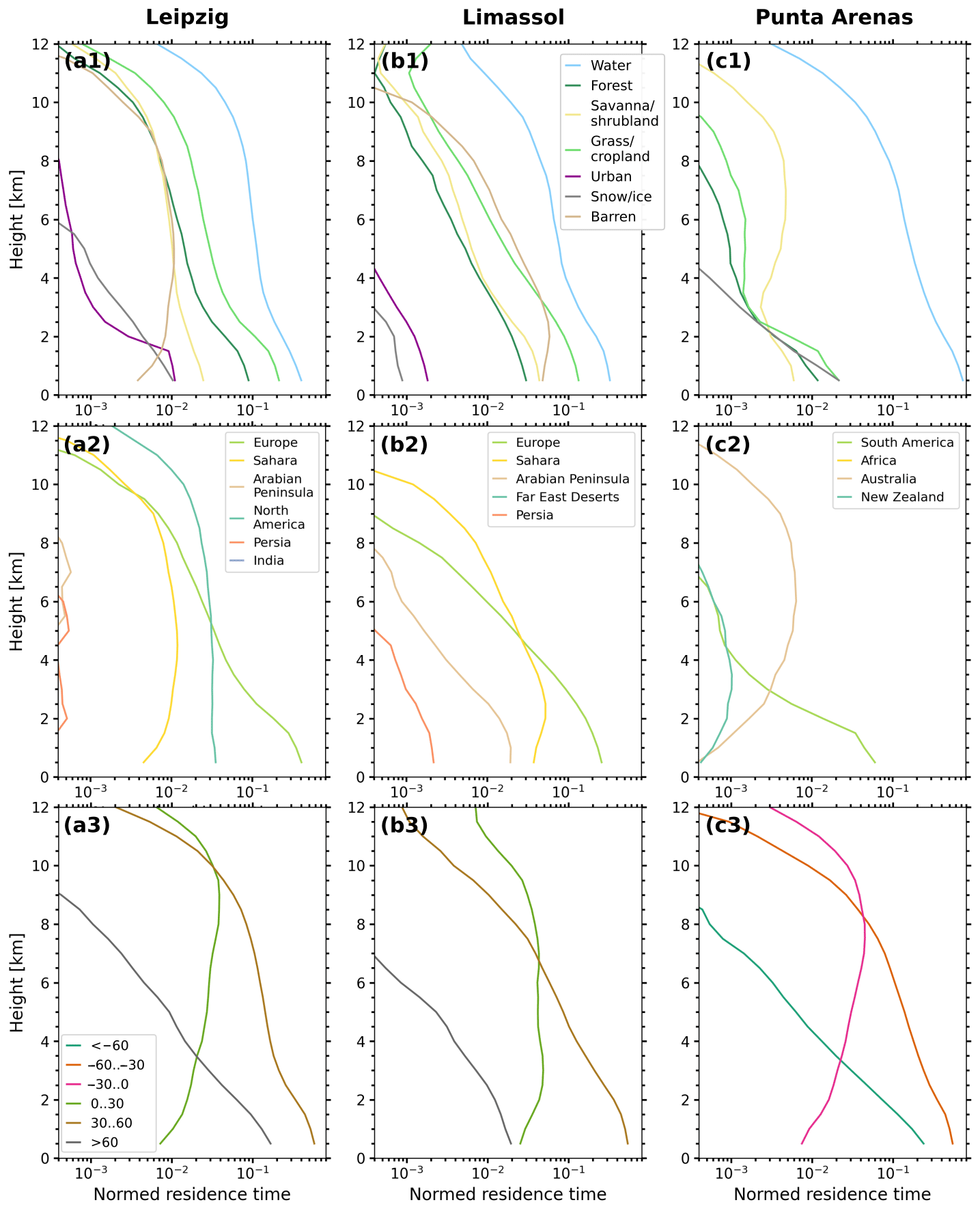
Figure B1Mean normalized residence time profile at (a) Leipzig, (b) Limassol, and (c) Punta Arenas for a reception height of 2 km. Residence times are shown for the surface cover classification (1), named areas (2), and latitude bands (3).

Figure B2Mean normalized residence time binned by temperature at (a) Leipzig, (b) Limassol, and (c) Punta Arenas for a reception height of 2 km. Residence times are shown for the surface cover classification (1), named areas (2), and latitude bands (3). Hatching indicates bins with less than 1 % of the values.
The automated time–height-resolved air mass source attribution described by Radenz et al. (2021) is used to characterize air mass origin for the LACROS observations. As in the original publication, 10 d HYSPLIT ensemble backward trajectories are calculated in intervals of 3 h and 500 m throughout the period of the deployment. For the calculation of the residence times, a reception height of 2 km is used. Additionally to the MODIS-based surface cover classification and the named geography (individually for Leipzig, Limassol, and Punta Arenas), 30∘ wide bands of latitude are used to characterize meridional transport. The assignment of the surface cover classed and named geography is depicted in Figs. 2 and 3 of Radenz et al. (2021). The average residence time for each set of surface types is shown in Fig. B1. However, as for the aerosol optical properties, geometrical height is less insightful than temperature. Thus, the residence time at each 3 h profile is binned by ambient temperature, using analysis profiles. Then, the average residence time is calculated per temperature bin (Fig. B2).
The Cloudnet datasets are provided by the ACTRIS Data Centre node for cloud profiling via the following links: https://hdl.handle.net/21.12132/2.e130b236928a4932 (Leipzig, last access: 20 October 2021), https://hdl.handle.net/21.12132/2.a056a828a6b94d1f (Limassol, last access: 20 October 2021), and https://hdl.handle.net/21.12132/2.b6c194d7d33b448e (Punta Arenas, last access: 20 October 2021). In the upcoming future, the Doppler lidar and PollyNET datasets will also be available via ACTRIS. Meanwhile, they can be obtained upon request from polly@tropos.de. The Lidar data was processed withe the PollyNET processing chain (Yin and Baars, 2021). The source code of the cloud sniffer, the database of identified clouds, and analysis scripts are available at https://doi.org/10.5281/zenodo.5574997 (Radenz and Bühl, 2021) and require a setup of pyLARDA (https://doi.org/10.5281/zenodo.4721311; Bühl et al., 2021). AERONET photometer observations at Leipzig, Limassol, and Punta Arenas are available from the AERONET database (http://aeronet.gsfc.nasa.gov/, last access: 20 October 2021).
MR analyzed the data and drafted the manuscript. MR, PS, JB, HB, RE, BBG, REM, and FZ conducted the campaigns and operated LACROS. PS, MR, and JB generated the Cloudnet dataset. HB processed the PollyXT lidar data. PS, JB, and AA supervised the work and revised the manuscript. All authors jointly contributed to the paper and the scientific discussion.
The contact author has declared that neither they nor their co-authors have any competing interests.
Publisher's note: Copernicus Publications remains neutral with regard to jurisdictional claims in published maps and institutional affiliations.
The authors wish to thank TROPOS, Cyprus University of Technology and University of Magallanes, for their logistic and infrastructural support during the LACROS deployments. We furthermore thank Teresa Vogl, Willi Schimmel, Audrey Teisseire, Cristofer Jimenez, Heike Kalesse-Los, and Roland Schrödner for keeping LACROS operational at Punta Arenas. We gratefully acknowledge the ACTRIS Cloud Remote Sensing Unit for making the Cloudnet datasets publicly available. LACROS operations were supported by the European Union (EU) Horizon 2020 (ACTRIS; grant no. 654109) and the Seventh Framework Programme (BACCHUS; grant no. 603445). Observations at Leipzig were supported by the German Bundesministerium für Bildung und Forschung funded projects “High Definition Clouds and Precipitation for Climate Prediction – HD(CP)2” (grant nos. 01LK1503F,01LK1502I, 01LK1209C, and 01LK1212C). Parts of the CyCARE and DACAPO-PESO campaigns were funded by the Deutsche Forschungsgemeinschaft (DFG – German Research Foundation) project PICNICC (SE2464/1-1 and KA4162/2-1). Johannes Bühl acknowledges funding by DFG project COARSEMIX (398285025). Rodanthi-Elisabeth Mamouri has been financially supported by the SIROCCO project (grant no. EXCELLENCE/1216/0217), co-funded by the Republic of Cyprus and the structural funds of the EU for Cyprus through the Research and Innovation Foundation. We also acknowledge the EXCELSIOR EU H2020 Widespread Teaming programme, grant agreement no. 857510 (http://www.excelsior2020.eu, last access: 20 October 2021) and the Republic of Cyprus for the support of the establishment the ERATOSTHENES Centre of Excellence. Boris Barja González acknowledges funding by the ANID/CONICYT/FONDECYT Iniciación 11181335. Holger Baars acknowledges funding by the AEOLUS Cal/Val activities (German Bundesministeriums für Wirtschaft und Energie; grant no. 50EE1721C). We thank AERONET Europe for providing the calibration service of the photometer. The authors gratefully acknowledge the NOAA Air Resources Laboratory (ARL) for the provision of the HYSPLIT transport and dispersion model. We thank Timothy J. Dunkerton for serving as an editor and gratefully acknowledge the constructive comments of the two referees.
This research has been supported by the European Commission, H2020 Research Infrastructures (grant nos. 654109 and 857510), the EU Seventh Framework Programme (grant no. 603445), the German Bundesministerium für Bildung und Forschung funded projects “High Definition Clouds and Precipitation for Climate Prediction HD(CP)2” (grant nos. 01LK1503F, 01LK1502I, 01LK1209C, and 01LK1212C), the DFG (grant nos. SE2464/1-1, KA4162/2-1, and 39828502), EU/Cyprus Research and Innovation Foundation EXCELLENCE/1216/0217, ANID/CONICYT/FONDECYT Iniciación (grant no. 11181335), and the German Bundesministerium für Wirtschaft und Energie (grant no. 50EE1721C).
This paper was edited by Timothy J. Dunkerton and reviewed by two anonymous referees.
Achtert, P., O'Connor, E. J., Brooks, I. M., Sotiropoulou, G., Shupe, M. D., Pospichal, B., Brooks, B. J., and Tjernström, M.: Properties of Arctic liquid and mixed-phase clouds from shipborne Cloudnet observations during ACSE 2014, Atmos. Chem. Phys., 20, 14983–15002, https://doi.org/10.5194/acp-20-14983-2020, 2020. a
Acquistapace, C., Löhnert, U., Maahn, M., and Kollias, P.: A New Criterion to Improve Operational Drizzle Detection with Ground-Based Remote Sensing, J. Atmos. Ocean. Tech., 36, 781–801, https://doi.org/10.1175/JTECH-D-18-0158.1, 2019. a
Alexander, S. P. and Protat, A.: Cloud Properties Observed From the Surface and by Satellite at the Northern Edge of the Southern Ocean, J. Geophys. Res.-Atmos., 123, 443–456, https://doi.org/10.1002/2017JD026552, 2018. a, b
Alexander, S. P. and Protat, A.: Vertical Profiling of Aerosols With a Combined Raman-Elastic Backscatter Lidar in the Remote Southern Ocean Marine Boundary Layer (43–66∘S, 132–150∘E), J. Geophys. Res.-Atmos., 124, 12107–12125, https://doi.org/10.1029/2019JD030628, 2019. a
Alexander, S. P., Sato, K., Watanabe, S., Kawatani, Y., and Murphy, D. J.: Southern Hemisphere Extratropical Gravity Wave Sources and Intermittency Revealed by a Middle-Atmosphere General Circulation Model, J. Atmos. Sci., 73, 1335–1349, https://doi.org/10.1175/JAS-D-15-0149.1, 2016. a
Alexander, S. P., Orr, A., Webster, S., and Murphy, D. J.: Observations and fine-scale model simulations of gravity waves over Davis, East Antarctica (69∘ S, 78∘ E), J. Geophys. Res.-Atmos., 122, 7355–7370, https://doi.org/10.1002/2017JD026615, 2017. a
Alexander, S. P., McFarquhar, G. M., Marchand, R., Protat, A., Vignon, É., Mace, G. G., and Klekociuk, A. R.: Mixed-phase Clouds and Precipitation in Southern Ocean Cyclones and Cloud Systems Observed Poleward of 64∘S by Ship-based Cloud Radar and Lidar, J. Geophys. Res.-Atmos., https://doi.org/10.1029/2020JD033626, 2021. a
Althausen, D., Engelmann, R., Baars, H., Heese, B., Ansmann, A., Müller, D., and Komppula, M.: Portable Raman Lidar PollyXT for Automated Profiling of Aerosol Backscatter, Extinction, and Depolarization, J. Atmos. Ocean. Tech., 26, 2366–2378, https://doi.org/10.1175/2009JTECHA1304.1, 2009. a
Ansmann, A.: Ice Formation in Saharan Dust over Central Europe Observed with Temperature/Humidity/Aerosol Raman Lidar, J. Geophys. Res., 110, D18S12, https://doi.org/10.1029/2004JD005000, 2005. a
Ansmann, A., Bösenberg, J., Chaikovsky, A., Comerón, A., Eckhardt, S., Eixmann, R., Freudenthaler, V., Ginoux, P., Komguem, L., Linné, H., Márquez, M.Á. L., Matthias, V., Mattis, I., Mitev, V., Müller, D., Music, S., Nickovic, S., Pelon, J., Sauvage, L., Sobolewsky, P., Srivastava, M. K., Stohl, A., Torres, O., Vaughan, G., Wandinger, U., and Wiegner, M.: Long-range transport of Saharan dust to northern Europe: The 11–16 October 2001 outbreak observed with EARLINET, J. Geophys. Res.-Atmos., 108, AAC 12, https://doi.org/10.1029/2003JD003757, 2003. a
Ansmann, A., Mamouri, R.-E., Bühl, J., Seifert, P., Engelmann, R., Hofer, J., Nisantzi, A., Atkinson, J. D., Kanji, Z. A., Sierau, B., Vrekoussis, M., and Sciare, J.: Ice-nucleating particle versus ice crystal number concentrationin altocumulus and cirrus layers embedded in Saharan dust:a closure study, Atmos. Chem. Phys., 19, 15087–15115, https://doi.org/10.5194/acp-19-15087-2019, 2019. a, b
Baars, H., Kanitz, T., Engelmann, R., Althausen, D., Heese, B., Komppula, M., Preißler, J., Tesche, M., Ansmann, A., Wandinger, U., Lim, J.-H., Ahn, J. Y., Stachlewska, I. S., Amiridis, V., Marinou, E., Seifert, P., Hofer, J., Skupin, A., Schneider, F., Bohlmann, S., Foth, A., Bley, S., Pfüller, A., Giannakaki, E., Lihavainen, H., Viisanen, Y., Hooda, R. K., Pereira, S. N., Bortoli, D., Wagner, F., Mattis, I., Janicka, L., Markowicz, K. M., Achtert, P., Artaxo, P., Pauliquevis, T., Souza, R. A. F., Sharma, V. P., van Zyl, P. G., Beukes, J. P., Sun, J., Rohwer, E. G., Deng, R., Mamouri, R.-E., and Zamorano, F.: An overview of the first decade of PollyNET: an emerging network of automated Raman-polarization lidars for continuous aerosol profiling, Atmos. Chem. Phys., 16, 5111–5137, https://doi.org/10.5194/acp-16-5111-2016, 2016. a, b, c
Baars, H., Seifert, P., Engelmann, R., and Wandinger, U.: Target categorization of aerosol and clouds by continuous multiwavelength-polarization lidar measurements, Atmos. Meas. Tech., 10, 3175–3201, https://doi.org/10.5194/amt-10-3175-2017, 2017. a, b
Baars, H., Radenz, M., Floutsi, A. A., Engelmann, R., Althausen, D., Heese, B., Ansmann, A., Flament, T., Dabas, A., Trapon, D., Reitebuch, O., Bley, S., and Wandinger, U.: Californian Wildfire Smoke Over Europe: A First Example of the Aerosol Observing Capabilities of Aeolus Compared to Ground-Based Lidar, Geophys. Res. Lett., 48, e2020GL092194, https://doi.org/10.1029/2020GL092194, 2021. a
Baker, B. A. and Lawson, R. P.: In Situ Observations of the Microphysical Properties of Wave, Cirrus, and Anvil Clouds. Part I: Wave Clouds, J. Atmos. Sci., 63, 3160–3185, https://doi.org/10.1175/JAS3802.1, 2006. a
Barreto, Á., Cuevas, E., Granados-Muñoz, M.-J., Alados-Arboledas, L., Romero, P. M., Gröbner, J., Kouremeti, N., Almansa, A. F., Stone, T., Toledano, C., Román, R., Sorokin, M., Holben, B., Canini, M., and Yela, M.: The new sun-sky-lunar Cimel CE318-T multiband photometer – a comprehensive performance evaluation, Atmos. Meas. Tech., 9, 631–654, https://doi.org/10.5194/amt-9-631-2016, 2016. a
Bodas-Salcedo, A., Williams, K. D., Ringer, M. A., Beau, I., Cole, J. N. S., Dufresne, J.-L., Koshiro, T., Stevens, B., Wang, Z., and Yokohata, T.: Origins of the Solar Radiation Biases over the Southern Ocean in CFMIP2 Models, J. Climate, 27, 41–56, https://doi.org/10.1175/JCLI-D-13-00169.1, 2014. a
Bodas-Salcedo, A., Hill, P., Furtado, K., Williams, K., Field, P., Manners, J., Hyder, P., and Kato, S.: Large contribution of supercooled liquid clouds to the solar radiation budget of the Southern Ocean, J. Climate, 29, 4213–4228, 2016. a
Bohlmann, S., Baars, H., Radenz, M., Engelmann, R., and Macke, A.: Ship-borne aerosol profiling with lidar over the Atlantic Ocean: from pure marine conditions to complex dust–smoke mixtures, Atmos. Chem. Phys., 18, 9661–9679, https://doi.org/10.5194/acp-18-9661-2018, 2018. a, b
Bourgeois, Q., Ekman, A. M. L., Renard, J.-B., Krejci, R., Devasthale, A., Bender, F. A.-M., Riipinen, I., Berthet, G., and Tackett, J. L.: How much of the global aerosol optical depth is found in the boundary layer and free troposphere?, Atmos. Chem. Phys., 18, 7709–7720, https://doi.org/10.5194/acp-18-7709-2018, 2018. a
Bromwich, D. H., Werner, K., Casati, B., Powers, J. G., Gorodetskaya, I. V., Massonnet, F., Vitale, V., Heinrich, V. J., Liggett, D., Arndt, S., Barja, B., Bazile, E., Carpentier, S., Carrasco, J. F., Choi, T., Choi, Y., Colwell, S. R., Cordero, R. R., Gervasi, M., Haiden, T., Hirasawa, N., Inoue, J., Jung, T., Kalesse, H., Kim, S.-J., Lazzara, M. A., Manning, K. W., Norris, K., Park, S.-J., Reid, P., Rigor, I., Rowe, P. M., Schmithüsen, H., Seifert, P., Sun, Q., Uttal, T., Zannoni, M., and Zou, X.: The Year of Polar Prediction in the Southern Hemisphere (YOPP-SH), B. Am. Meteorol. Soc., 101, E1653–E1676, https://doi.org/10.1175/BAMS-D-19-0255.1, 2020. a, b
Bühl, J., Ansmann, A., Seifert, P., Baars, H., and Engelmann, R.: Toward a quantitative characterization of heterogeneous ice formation with lidar/radar: Comparison of CALIPSO/CloudSat with ground-based observations, Geophys. Res. Lett., 40, 4404–4408, https://doi.org/10.1002/grl.50792, 2013a. a, b, c, d, e
Bühl, J., Seifert, P., Wandinger, U., Baars, H., Kanitz, T., Schmidt, J., Myagkov, A., Engelmann, R., Skupin, A., Heese, B., Klepel, A., Althausen, D., and Ansmann, A.: LACROS: The Leipzig Aerosol and Cloud Remote Observations System, in: SPIE Remote Sensing, edited by: Comeron, A., Kassianov, E. I., Schäfer, K., Stein, K., and Gonglewski, J. D., p. 889002, Dresden, Germany, https://doi.org/10.1117/12.2030911, 2013b. a
Bühl, J., Seifert, P., Myagkov, A., and Ansmann, A.: Measuring ice- and liquid-water properties in mixed-phase cloud layers at the Leipzig Cloudnet station, Atmos. Chem. Phys., 16, 10609–10620, https://doi.org/10.5194/acp-16-10609-2016, 2016. a, b, c, d, e, f, g, h, i
Bühl, J., Seifert, P., Engelmann, R., and Ansmann, A.: Impact of vertical air motions on ice formation rate in mixed-phase cloud layers, npj Climate and Atmospheric Science, 2, 36, https://doi.org/10.1038/s41612-019-0092-6, 2019. a, b, c
Bühl, J., Radenz, M., Schimmel, W., Vogl, T., Röttenbacher, J., and Lochmann, M.: pyLARDA v3.2, Zenodo [code], https://doi.org/10.5281/zenodo.4721311, 2021. a, b
Choi, Y.-S., Lindzen, R. S., Ho, C.-H., and Kim, J.: Space observations of cold-cloud phase change, P. Natl. Acad. Sci. USA, 107, 11211–11216, https://doi.org/10.1073/pnas.1006241107, 2010. a, b, c, d
Cotton, R. J. and Field, P. R.: Ice nucleation characteristics of an isolated wave cloud, Q. J. Roy. Meteor. Soc., 128, 2417–2437, https://doi.org/10.1256/qj.01.150, 2002. a
Crewell, S. and Löhnert, U.: Accuracy of Boundary Layer Temperature Profiles Retrieved With Multifrequency Multiangle Microwave Radiometry, IEEE T. Geosci. Remote, 45, 2195–2201, https://doi.org/10.1109/TGRS.2006.888434, 2007. a
D'Alessandro, J. J., Diao, M., Wu, C., Liu, X., Jensen, J. B., and Stephens, B. B.: Cloud Phase and Relative Humidity Distributions over the Southern Ocean in Austral Summer Based on In Situ Observations and CAM5 Simulations, J. Climate, 32, 2781–2805, https://doi.org/10.1175/JCLI-D-18-0232.1, 2019. a
de Boer, G., Eloranta, E. W., and Shupe, M. D.: Arctic Mixed-Phase Stratiform Cloud Properties from Multiple Years of Surface-Based Measurements at Two High-Latitude Locations, J. Atmos. Sci., 66, 2874–2887, https://doi.org/10.1175/2009JAS3029.1, 2009. a
DeMott, P. J., Prenni, A. J., Liu, X., Kreidenweis, S. M., Petters, M. D., Twohy, C. H., Richardson, M. S., Eidhammer, T., and Rogers, D. C.: Predicting global atmospheric ice nuclei distributions and their impacts on climate, P. Natl. Acad. Sci. USA, 107, 11217–11222, https://doi.org/10.1073/pnas.0910818107, 2010. a
DeMott, P. J., Prenni, A. J., McMeeking, G. R., Sullivan, R. C., Petters, M. D., Tobo, Y., Niemand, M., Möhler, O., Snider, J. R., Wang, Z., and Kreidenweis, S. M.: Integrating laboratory and field data to quantify the immersion freezing ice nucleation activity of mineral dust particles, Atmos. Chem. Phys., 15, 393–409, https://doi.org/10.5194/acp-15-393-2015, 2015. a
Desai, N., Chandrakar, K. K., Kinney, G., Cantrell, W., and Shaw, R. A.: Aerosol-Mediated Glaciation of Mixed-Phase Clouds: Steady-State Laboratory Measurements, Geophys. Res. Lett., 46, 9154–9162, https://doi.org/10.1029/2019GL083503, 2019. a
Durant, A. J.: Evaporation Freezing by Contact Nucleation Inside-Out, Geophys. Res. Lett., 32, L20814, https://doi.org/10.1029/2005GL024175, 2005. a
Engelmann, R., Kanitz, T., Baars, H., Heese, B., Althausen, D., Skupin, A., Wandinger, U., Komppula, M., Stachlewska, I. S., Amiridis, V., Marinou, E., Mattis, I., Linné, H., and Ansmann, A.: The automated multiwavelength Raman polarization and water-vapor lidar PollyXT: the neXT generation, Atmos. Meas. Tech., 9, 1767–1784, https://doi.org/10.5194/amt-9-1767-2016, 2016. a, b, c, d
Fan, J., Wang, Y., Rosenfeld, D., and Liu, X.: Review of Aerosol–Cloud Interactions: Mechanisms, Significance, and Challenges, J. Atmos. Sci., 73, 4221–4252, https://doi.org/10.1175/JAS-D-16-0037.1, 2016. a
Fang, M., Albrecht, B. A., Ghate, V. P., and Kollias, P.: Turbulence in Continental Stratocumulus, Part I: External Forcings and Turbulence Structures, Bound.-Lay. Meteorol., 150, 341–360, https://doi.org/10.1007/s10546-013-9873-3, 2014. a
Fernald, F. G.: Analysis of Atmospheric Lidar Observations: Some Comments, Appl. Optics, 23, 652–653, 1984. a
Field, P. R., Heymsfield, A. J., Shipway, B. J., DeMott, P. J., Pratt, K. A., Rogers, D. C., Stith, J., and Prather, K. A.: Ice in Clouds Experiment–Layer Clouds. Part II: Testing Characteristics of Heterogeneous Ice Formation in Lee Wave Clouds, J. Atmos. Sci., 69, 1066–1079, https://doi.org/10.1175/JAS-D-11-026.1, 2012. a
Floutsi, A. A., Baars, H., Radenz, M., Haarig, M., Yin, Z., Seifert, P., Jimenez, C., Ansmann, A., Engelmann, R., Barja, B., Zamorano, F., and Wandinger, U.: Advection of Biomass Burning Aerosols towards the Southern Hemispheric Mid-Latitude Station of Punta Arenas as Observed with Multiwavelength Polarization Raman Lidar, Remote Sens.-Basel, 13, 138, https://doi.org/10.3390/rs13010138, 2021. a, b, c
Foth, A., Kanitz, T., Engelmann, R., Baars, H., Radenz, M., Seifert, P., Barja, B., Fromm, M., Kalesse, H., and Ansmann, A.: Vertical aerosol distribution in the southern hemispheric midlatitudes as observed with lidar in Punta Arenas, Chile (53.2∘ S and 70.9∘ W), during ALPACA, Atmos. Chem. Phys., 19, 6217–6233, https://doi.org/10.5194/acp-19-6217-2019, 2019. a, b
Franklin, C. N., Sun, Z., Bi, D., Dix, M., Yan, H., and Bodas-Salcedo, A.: Evaluation of clouds in ACCESS using the satellite simulator package COSP: Global, seasonal, and regional cloud properties, J. Geophys. Res.-Atmos., 118, 732–748, https://doi.org/10.1029/2012JD018469, 2013. a
Fukuta, N. and Takahashi, T.: The Growth of Atmospheric Ice Crystals: A Summary of Findings in Vertical Supercooled Cloud Tunnel Studies, J. Atmos. Sci., 56, 1963–1979, https://doi.org/10.1175/1520-0469(1999)056<1963:TGOAIC>2.0.CO;2, 1999. a, b
Gong, X., Radenz, M., Wex, H., Seifert, P., Ataei, F., Henning, S., Baars, H., Barja, B., Ansmann, A., and Stratmann, F.: A significant land source of ice-nucleating particles at the tip of Chile's southernmost Patagonia region, Atmos. Chem. Phys. Discuss., in preparation, 2021. a
Görsdorf, U., Lehmann, V., Bauer-Pfundstein, M., Peters, G., Vavriv, D., Vinogradov, V., and Volkov, V.: A 35-GHz Polarimetric Doppler Radar for Long-Term Observations of Cloud Parameters–Description of System and Data Processing, J. Atmos. Ocean. Tech., 32, 675–690, https://doi.org/10.1175/JTECH-D-14-00066.1, 2015. a
Griesche, H. J., Ohneiser, K., Seifert, P., Radenz, M., Engelmann, R., and Ansmann, A.: Contrasting ice formation in Arctic clouds: surface-coupled vs. surface-decoupled clouds, Atmos. Chem. Phys., 21, 10357–10374, https://doi.org/10.5194/acp-21-10357-2021, 2021. a
Grise, K. M., Polvani, L. M., and Fasullo, J. T.: Reexamining the Relationship between Climate Sensitivity and the Southern Hemisphere Radiation Budget in CMIP Models, J. Climate, 28, 9298–9312, https://doi.org/10.1175/JCLI-D-15-0031.1, 2015. a
Haarig, M., Ansmann, A., Gasteiger, J., Kandler, K., Althausen, D., Baars, H., Radenz, M., and Farrell, D. A.: Dry versus wet marine particle optical properties: RH dependence of depolarization ratio, backscatter, and extinction from multiwavelength lidar measurements during SALTRACE, Atmos. Chem. Phys., 17, 14199–14217, https://doi.org/10.5194/acp-17-14199-2017, 2017. a
Haarig, M., Ansmann, A., Baars, H., Jimenez, C., Veselovskii, I., Engelmann, R., and Althausen, D.: Depolarization and lidar ratios at 355, 532, and 1064 nm and microphysical properties of aged tropospheric and stratospheric Canadian wildfire smoke, Atmos. Chem. Phys., 18, 11847–11861, https://doi.org/10.5194/acp-18-11847-2018, 2018. a
Hall, W. D. and Pruppacher, H. R.: The Survival of Ice Particles Falling from Cirrus Clouds in Subsaturated Air, J. Atmos. Sci., 33, 1995–2006, https://doi.org/10.1175/1520-0469(1976)033<1995:TSOIPF>2.0.CO;2, 1976. a
Hamilton, D. S., Lee, L. A., Pringle, K. J., Reddington, C. L., Spracklen, D. V., and Carslaw, K. S.: Occurrence of pristine aerosol environments on a polluted planet, P. Natl. Acad. Sci. USA, 111, 18466–18471, https://doi.org/10.1073/pnas.1415440111, 2014. a, b
Haynes, J. M., Jakob, C., Rossow, W. B., Tselioudis, G., and Brown, J.: Major Characteristics of Southern Ocean Cloud Regimes and Their Effects on the Energy Budget, J. Climate, 24, 5061–5080, https://doi.org/10.1175/2011JCLI4052.1, 2011. a
Heymsfield, A. J. and Miloshevich, L. M.: Homogeneous Ice Nucleation and Supercooled Liquid Water in Orographic Wave Clouds, J. Atmos. Sci., 50, 2335–2353, https://doi.org/10.1175/1520-0469(1993)050<2335:HINASL>2.0.CO;2, 1993. a, b
Hogan, R. J. and O'Connor, E. J.: Facilitating cloud radar and lidar algorithms: the Cloudnet Instrument Synergy/Target Categorization product, Tech. rep., University of Reading, Department of Meteorology, available at: http://www.met.rdg.ac.uk/~swrhgnrj/publications/categorization.pdf (last access: 20 October 2021), 2004. a
Hogan, R. J., Mittermaier, M. P., and Illingworth, A. J.: The Retrieval of Ice Water Content from Radar Reflectivity Factor and Temperature and Its Use in Evaluating a Mesoscale Model, J. Appl. Meteorol. Clim., 45, 301–317, https://doi.org/10.1175/jam2340.1, 2006. a, b, c
Hu, Y., Rodier, S., Xu, K.-m., Sun, W., Huang, J., Lin, B., Zhai, P., and Josset, D.: Occurrence, liquid water content, and fraction of supercooled water clouds from combined CALIOP/IIR/MODIS measurements, J. Geophys. Res.-Atmos., 115, D00H34, https://doi.org/10.1029/2009JD012384, 2010. a, b
Huang, Y., Protat, A., Siems, S. T., and Manton, M. J.: A-Train Observations of Maritime Midlatitude Storm-Track Cloud Systems: Comparing the Southern Ocean against the North Atlantic, J. Climate, 28, 1920–1939, https://doi.org/10.1175/JCLI-D-14-00169.1, 2015. a
Huang, Y., Chubb, T., Baumgardner, D., deHoog, M., Siems, S. T., and Manton, M. J.: Evidence for Secondary Ice Production in Southern Ocean Open Cellular Convection: Secondary Ice Production over the Southern Ocean, Q. J. Roy. Meteor. Soc., 143, 1685–1703, https://doi.org/10.1002/qj.3041, 2017. a
Hyder, P., Edwards, J. M., Allan, R. P., Hewitt, H. T., Bracegirdle, T. J., Gregory, J. M., Wood, R. A., Meijers, A. J. S., Mulcahy, J., Field, P., Furtado, K., Bodas-Salcedo, A., Williams, K. D., Copsey, D., Josey, S. A., Liu, C., Roberts, C. D., Sanchez, C., Ridley, J., Thorpe, L., Hardiman, S. C., Mayer, M., Berry, D. I., and Belcher, S. E.: Critical Southern Ocean Climate Model Biases Traced to Atmospheric Model Cloud Errors, Nat. Commun., 9, 3625, https://doi.org/10.1038/s41467-018-05634-2, 2018. a
Illingworth, A. J., Hogan, R. J., O'Connor, E., Bouniol, D., Brooks, M. E., Delanoé, J., Donovan, D. P., Eastment, J. D., Gaussiat, N., Goddard, J. W. F., Haeffelin, M., Baltink, H. K., Krasnov, O. A., Pelon, J., Piriou, J.-M., Protat, A., Russchenberg, H. W. J., Seifert, A., Tompkins, A. M., van Zadelhoff, G.-J., Vinit, F., Willén, U., Wilson, D. R., and Wrench, C. L.: Cloudnet: Continuous Evaluation of Cloud Profiles in Seven Operational Models Using Ground-Based Observations, B. Am. Meteorol. Soc., 88, 883–898, https://doi.org/10.1175/BAMS-88-6-883, 2007. a
Jimenez, C., Ansmann, A., Engelmann, R., Donovan, D., Malinka, A., Seifert, P., Wiesen, R., Radenz, M., Yin, Z., Bühl, J., Schmidt, J., Barja, B., and Wandinger, U.: The dual-field-of-view polarization lidar technique: a new concept in monitoring aerosol effects in liquid-water clouds – case studies, Atmos. Chem. Phys., 20, 15265–15284, https://doi.org/10.5194/acp-20-15265-2020, 2020. a, b
Kanitz, T., Seifert, P., Ansmann, A., Engelmann, R., Althausen, D., Casiccia, C., and Rohwer, E. G.: Contrasting the impact of aerosols at northern and southern midlatitudes on heterogeneous ice formation, Geophys. Res. Lett., 38, L17802, https://doi.org/10.1029/2011gl048532, 2011. a, b, c, d, e, f, g, h
Kanji, Z. A., Ladino, L. A., Wex, H., Boose, Y., Burkert-Kohn, M., Cziczo, D. J., and Krämer, M.: Overview of Ice Nucleating Particles, Meteor. Mon., 58, 1.1–1.33, https://doi.org/10.1175/AMSMONOGRAPHS-D-16-0006.1, 2017. a, b
Kay, J. E., Bourdages, L., Miller, N. B., Morrison, A., Yettella, V., Chepfer, H., and Eaton, B.: Evaluating and improving cloud phase in the Community Atmosphere Model version 5 using spaceborne lidar observations, J. Geophys. Res.-Atmos., 121, 4162–4176, https://doi.org/10.1002/2015JD024699, 2016. a
Korolev, A.: Limitations of the Wegener–Bergeron–Findeisen Mechanism in the Evolution of Mixed-Phase Clouds, J. Atmos. Sci., 64, 3372–3375, https://doi.org/10.1175/JAS4035.1, 2007. a, b
Kuma, P., McDonald, A. J., Morgenstern, O., Alexander, S. P., Cassano, J. J., Garrett, S., Halla, J., Hartery, S., Harvey, M. J., Parsons, S., Plank, G., Varma, V., and Williams, J.: Evaluation of Southern Ocean cloud in the HadGEM3 general circulation model and MERRA-2 reanalysis using ship-based observations, Atmos. Chem. Phys., 20, 6607–6630, https://doi.org/10.5194/acp-20-6607-2020, 2020. a, b
Liu, Y., Geerts, B., Miller, M., Daum, P., and McGraw, R.: Threshold Radar Reflectivity for Drizzling Clouds, Geophys. Res. Lett., 35, L03807, https://doi.org/10.1029/2007GL031201, 2008. a
Löffler-Mang, M. and Joss, J.: An Optical Disdrometer for Measuring Size and Velocity of Hydrometeors, J. Atmos. Ocean. Tech., 17, 130–139, https://doi.org/10.1175/1520-0426(2000)017<0130:AODFMS>2.0.CO;2, 2000. a
Mace, G. G. and Protat, A.: Clouds over the Southern Ocean as Observed from the R/V Investigator during CAPRICOR N. Part I: Cloud Occurrence and Phase Partitioning, J. Appl. Meteorol. Clim., 57, 1783–1803, https://doi.org/10.1175/JAMC-D-17-0194.1, 2018. a
Mace, G. G., Benson, S., and Hu, Y.: On the Frequency of Occurrence of the Ice Phase in Supercooled Southern Ocean Low Clouds Derived From CALIPSO and CloudSat, Geophys. Res. Lett., 47, e2020GL087554, https://doi.org/10.1029/2020GL087554, 2020. a
Mamouri, R.-E. and Ansmann, A.: Potential of polarization lidar to provide profiles of CCN- and INP-relevant aerosol parameters, Atmos. Chem. Phys., 16, 5905–5931, https://doi.org/10.5194/acp-16-5905-2016, 2016. a, b
Mamouri, R.-E. and Ansmann, A.: Potential of polarization/Raman lidar to separate fine dust, coarse dust, maritime, and anthropogenic aerosol profiles, Atmos. Meas. Tech., 10, 3403–3427, https://doi.org/10.5194/amt-10-3403-2017, 2017. a
McCluskey, C. S., Hill, T. C. J., Humphries, R. S., Rauker, A. M., Moreau, S., Strutton, P. G., Chambers, S. D., Williams, A. G., McRobert, I., Ward, J., Keywood, M. D., Harnwell, J., Ponsonby, W., Loh, Z. M., Krummel, P. B., Protat, A., Kreidenweis, S. M., and DeMott, P. J.: Observations of Ice Nucleating Particles Over Southern Ocean Waters, Geophys. Res. Lett., 45, 11989–11997, https://doi.org/10.1029/2018GL079981, 2018a. a
McCluskey, C. S., Ovadnevaite, J., Rinaldi, M., Atkinson, J., Belosi, F., Ceburnis, D., Marullo, S., Hill, T. C. J., Lohmann, U., Kanji, Z. A., O'Dowd, C., Kreidenweis, S. M., and DeMott, P. J.: Marine and Terrestrial Organic Ice-Nucleating Particles in Pristine Marine to Continentally Influenced Northeast Atlantic Air Masses, J. Geophys. Res.-Atmos., 123, 6196–6212, https://doi.org/10.1029/2017JD028033, 2018b. a
McErlich, C., McDonald, A., Schuddeboom, A., and Silber, I.: Comparing Satellite- and Ground-Based Observations of Cloud Occurrence Over High Southern Latitudes, J. Geophys. Res.-Atmos., 126, e2020JD033607, https://doi.org/10.1029/2020JD033607, 2021. a
McFarquhar, G. M., Bretherton, C. S., Marchand, R., Protat, A., DeMott, P. J., Alexander, S. P., Roberts, G. C., Twohy, C. H., Toohey, D., Siems, S., Huang, Y., Wood, R., Rauber, R. M., Lasher-Trapp, S., Jensen, J., Stith, J. L., Mace, J., Um, J., Järvinen, E., Schnaiter, M., Gettelman, A., Sanchez, K. J., McCluskey, C. S., Russell, L. M., McCoy, I. L., Atlas, R. L., Bardeen, C. G., Moore, K. A., Hill, T. C. J., Humphries, R. S., Keywood, M. D., Ristovski, Z., Cravigan, L., Schofield, R., Fairall, C., Mallet, M. D., Kreidenweis, S. M., Rainwater, B., D'Alessandro, J., Wang, Y., Wu, W., Saliba, G., Levin, E. J. T., Ding, S., Lang, F., Truong, S. C. H., Wolff, C., Haggerty, J., Harvey, M. J., Klekociuk, A. R., and McDonald, A.: Observations of Clouds, Aerosols, Precipitation, and Surface Radiation over the Southern Ocean: An Overview of CAPRICORN, MARCUS, MICRE, and SOCRATES, B. Am. Meteorol. Soc., 102, E894–E928, https://doi.org/10.1175/BAMS-D-20-0132.1, 2021. a, b, c
Müller, D., Ansmann, A., Mattis, I., Tesche, M., Wandinger, U., Althausen, D., and Pisani, G.: Aerosol-Type-Dependent Lidar Ratios Observed with Raman Lidar, J. Geophys. Res., 112, D16202, https://doi.org/10.1029/2006JD008292, 2007. a
Murphy, D. M., Froyd, K. D., Bian, H., Brock, C. A., Dibb, J. E., DiGangi, J. P., Diskin, G., Dollner, M., Kupc, A., Scheuer, E. M., Schill, G. P., Weinzierl, B., Williamson, C. J., and Yu, P.: The distribution of sea-salt aerosol in the global troposphere, Atmos. Chem. Phys., 19, 4093–4104, https://doi.org/10.5194/acp-19-4093-2019, 2019. a
Myagkov, A., Seifert, P., Bauer-Pfundstein, M., and Wandinger, U.: Cloud radar with hybrid mode towards estimation of shape and orientation of ice crystals, Atmos. Meas. Tech., 9, 469–489, https://doi.org/10.5194/amt-9-469-2016, 2016. a, b
Naud, C. M., Booth, J. F., and Del Genio, A. D.: Evaluation of ERA-interim and MERRA cloudiness in the Southern Ocean, J. Climate, 27, 2109–2124, https://doi.org/10.1175/JCLI-D-13-00432.1, 2014. a
Nisantzi, A., Mamouri, R. E., Ansmann, A., Schuster, G. L., and Hadjimitsis, D. G.: Middle East versus Saharan dust extinction-to-backscatter ratios, Atmos. Chem. Phys., 15, 7071–7084, https://doi.org/10.5194/acp-15-7071-2015, 2015. a
Norgren, M. S., de Boer, G., and Shupe, M. D.: Observed aerosol suppression of cloud ice in low-level Arctic mixed-phase clouds, Atmos. Chem. Phys., 18, 13345–13361, https://doi.org/10.5194/acp-18-13345-2018, 2018. a
Ohneiser, K., Ansmann, A., Baars, H., Seifert, P., Barja, B., Jimenez, C., Radenz, M., Teisseire, A., Floutsi, A., Haarig, M., Foth, A., Chudnovsky, A., Engelmann, R., Zamorano, F., Bühl, J., and Wandinger, U.: Smoke of extreme Australian bushfires observed in the stratosphere over Punta Arenas, Chile, in January 2020: optical thickness, lidar ratios, and depolarization ratios at 355 and 532 nm, Atmos. Chem. Phys., 20, 8003–8015, https://doi.org/10.5194/acp-20-8003-2020, 2020. a, b, c
Pearson, G., Davies, F., and Collier, C.: An Analysis of the Performance of the UFAM Pulsed Doppler Lidar for Observing the Boundary Layer, J. Atmos. Ocean. Tech., 26, 240–250, https://doi.org/10.1175/2008JTECHA1128.1, 2009. a
Possner, A., Ekman, A. M. L., and Lohmann, U.: Cloud response and feedback processes in stratiform mixed-phase clouds perturbed by ship exhaust, Geophys. Res. Lett., 44, 1964–1972, https://doi.org/10.1002/2016GL071358, 2017. a
Radenz, M. and Bühl, J.: larda cloud sniffer, Zenodo [data set and code], https://doi.org/10.5281/zenodo.5574997, 2021. a
Radenz, M., Seifert, P., Baars, H., Floutsi, A. A., Yin, Z., and Bühl, J.: Automated time–height-resolved air mass source attribution for profiling remote sensing applications, Atmos. Chem. Phys., 21, 3015–3033, https://doi.org/10.5194/acp-21-3015-2021, 2021. a, b, c, d
Rose, T., Crewell, S., Löhnert, U., and Simmer, C.: A Network Suitable Microwave Radiometer for Operational Monitoring of the Cloudy Atmosphere, Atmos. Res., 75, 183–200, https://doi.org/10.1016/j.atmosres.2004.12.005, 2005. a
Sato, K., Tateno, S., Watanabe, S., and Kawatani, Y.: Gravity Wave Characteristics in the Southern Hemisphere Revealed by a High-Resolution Middle-Atmosphere General Circulation Model, J. Atmos. Sci., 69, 1378–1396, https://doi.org/10.1175/JAS-D-11-0101.1, 2012. a
Seifert, A., Köhler, C., and Beheng, K. D.: Aerosol-cloud-precipitation effects over Germany as simulated by a convective-scale numerical weather prediction model, Atmos. Chem. Phys., 12, 709–725, https://doi.org/10.5194/acp-12-709-2012, 2012. a
Seifert, P., Ansmann, A., Mattis, I., Wandinger, U., Tesche, M., Engelmann, R., Müller, D., Pérez, C., and Haustein, K.: Saharan dust and heterogeneous ice formation: Eleven years of cloud observations at a central European EARLINET site, J. Geophys. Res.-Atmos., 115, D20201, https://doi.org/10.1029/2009JD013222, 2010. a, b, c
Seifert, P., Kunz, C., Baars, H., Ansmann, A., Bühl, J., Senf, F., Engelmann, R., Althausen, D., and Artaxo, P.: Seasonal variability of heterogeneous ice formation in stratiform clouds over the Amazon Basin, Geophys. Res. Lett., 42, 5587–5593, https://doi.org/10.1002/2015gl064068, 2015. a, b, c
Seinfeld, J. H., Bretherton, C., Carslaw, K. S., Coe, H., DeMott, P. J., Dunlea, E. J., Feingold, G., Ghan, S., Guenther, A. B., Kahn, R., Kraucunas, I., Kreidenweis, S. M., Molina, M. J., Nenes, A., Penner, J. E., Prather, K. A., Ramanathan, V., Ramaswamy, V., Rasch, P. J., Ravishankara, A. R., Rosenfeld, D., Stephens, G., and Wood, R.: Improving Our Fundamental Understanding of the Role of Aerosol-cloud Interactions in the Climate System, P. Natl. Acad. Sci. USA, 113, 5781–5790, https://doi.org/10.1073/pnas.1514043113, 2016. a
Shao, Q., Randall, D. A., Moeng, C.-H., and Dickinson, R. E.: A Method to Determine the Amounts of Cloud-Top Radiative and Evaporative Cooling in a Stratocumulus-Topped Boundary Layer, Q. J. Roy. Meteor. Soc., 123, 2187–2213, https://doi.org/10.1002/qj.49712354403, 1997. a
Silber, I., Verlinde, J., Eloranta, E. W., and Cadeddu, M.: Antarctic Cloud Macrophysical, Thermodynamic Phase, and Atmospheric Inversion Coupling Properties at McMurdo Station: I. Principal Data Processing and Climatology, J. Geophys. Res.-Atmos., 123, 6099–6121, https://doi.org/10.1029/2018JD028279, 2018. a
Silber, I., Fridlind, A. M., Verlinde, J., Russell, L. M., and Ackerman, A. S.: Nonturbulent Liquid-Bearing Polar Clouds: Observed Frequency of Occurrence and Simulated Sensitivity to Gravity Waves, Geophys. Res. Lett., 47, e2020GL087099, https://doi.org/10.1029/2020GL087099, 2020. a, b, c
Simmel, M., Bühl, J., Ansmann, A., and Tegen, I.: Ice phase in altocumulus clouds over Leipzig: remote sensing observations and detailed modeling, Atmos. Chem. Phys., 15, 10453–10470, https://doi.org/10.5194/acp-15-10453-2015, 2015. a
Solomon, A., de Boer, G., Creamean, J. M., McComiskey, A., Shupe, M. D., Maahn, M., and Cox, C.: The relative impact of cloud condensation nuclei and ice nucleating particle concentrations on phase partitioning in Arctic mixed-phase stratocumulus clouds, Atmos. Chem. Phys., 18, 17047–17059, https://doi.org/10.5194/acp-18-17047-2018, 2018. a, b
Tan, I., Storelvmo, T., and Choi, Y.-S.: Spaceborne lidar observations of the ice-nucleating potential of dust, polluted dust, and smoke aerosols in mixed-phase clouds, J. Geophys. Res.-Atmos., 119, 6653–6665, https://doi.org/10.1002/2013JD021333, 2014. a, b
Trenberth, K. E. and Fasullo, J. T.: Simulation of Present-Day and Twenty-First-Century Energy Budgets of the Southern Oceans, J. Climate, 23, 440–454, https://doi.org/10.1175/2009JCLI3152.1, 2010. a
Uetake, J., Hill, T. C. J., Moore, K. A., DeMott, P. J., Protat, A., and Kreidenweis, S. M.: Airborne Bacteria Confirm the Pristine Nature of the Southern Ocean Boundary Layer, P. Natl. Acad. Sci. USA, 117, 13275–13282, https://doi.org/10.1073/pnas.2000134117, 2020. a
Vergara-Temprado, J., Murray, B. J., Wilson, T. W., O'Sullivan, D., Browse, J., Pringle, K. J., Ardon-Dryer, K., Bertram, A. K., Burrows, S. M., Ceburnis, D., DeMott, P. J., Mason, R. H., O'Dowd, C. D., Rinaldi, M., and Carslaw, K. S.: Contribution of feldspar and marine organic aerosols to global ice nucleating particle concentrations, Atmos. Chem. Phys., 17, 3637–3658, https://doi.org/10.5194/acp-17-3637-2017, 2017. a
Vignon, É., Alexander, S. P., DeMott, P. J., Sotiropoulou, G., Gerber, F., Hill, T. C. J., Marchand, R., Nenes, A., and Berne, A.: Challenging and Improving the Simulation of Mid-level Mixed-phase Clouds over the High-latitude Southern Ocean, J. Geophys. Res.-Atmos., https://doi.org/10.1029/2020JD033490, 2021. a
Villanueva, D., Heinold, B., Seifert, P., Deneke, H., Radenz, M., and Tegen, I.: The day-to-day co-variability between mineral dust and cloud glaciation: a proxy for heterogeneous freezing, Atmos. Chem. Phys., 20, 2177–2199, https://doi.org/10.5194/acp-20-2177-2020, 2020. a, b
Westbrook, C. D. and Illingworth, A. J.: The Formation of Ice in a Long-Lived Supercooled Layer Cloud, Q. J. Roy. Meteor. Soc., 139, 2209–2221, https://doi.org/10.1002/qj.2096, 2013. a
Wu, P., Dong, X., Xi, B., Tian, J., and Ward, D. M.: Profiles of MBL Cloud and Drizzle Microphysical Properties Retrieved From Ground-Based Observations and Validated by Aircraft In Situ Measurements Over the Azores, J. Geophys. Res.-Atmos., 125, e2019JD032205, https://doi.org/10.1029/2019JD032205, 2020. a
Yin, Z. and Baars, H.: PollyNET/Pollynet_Processing_Chain: Version 2.1, Zenodo [code], https://doi.org/10.5281/zenodo.4694451, 2021. a, b
Young, I.: Seasonal variability of the global ocean wind and wave climate, Int. J. Climatol., 19, 931–950, https://doi.org/10.1002/(SICI)1097-0088(199907)19:9<931::AID-JOC412>3.0.CO;2-O, 1999. a
Zaremba, T. J., Rauber, R. M., McFarquhar, G. M., Hayman, M., Finlon, J. A., and Stechman, D. M.: Phase Characterization of Cold Sector Southern Ocean Cloud Tops: Results from SOCRATES, J. Geophys. Res.-Atmos., 125, e2020JD033673, https://doi.org/10.1029/2020JD033673, 2020. a
Zhang, D., Wang, Z., Kollias, P., Vogelmann, A. M., Yang, K., and Luo, T.: Ice particle production in mid-level stratiform mixed-phase clouds observed with collocated A-Train measurements, Atmos. Chem. Phys., 18, 4317–4327, https://doi.org/10.5194/acp-18-4317-2018, 2018. a, b, c, d, e, f
- Abstract
- Introduction
- Data and methods
- Results
- Discussion of observed contrasts in properties of shallow clouds
- Summary and outlook
- Appendix A: Wave-cloud example
- Appendix B: Air mass source estimate
- Code and data availability
- Author contributions
- Competing interests
- Disclaimer
- Acknowledgements
- Financial support
- Review statement
- References