Limitations of the radon tracer method (RTM) to estimate regional greenhouse gas (GHG) emissions – a case study for methane in Heidelberg

Correlations of nighttime atmospheric methane (CH₄) and ²²²radon (²²²Rn) observations in Heidelberg, Germany, were evaluated with the radon tracer method (RTM) to estimate the trend of annual nocturnal CH₄ emissions from 1996–2020 in the footprint of the station. After an initial 30 % decrease in emissions from 1996 to 2004, there was no further systematic trend but small inter-annual variations were observed thereafter. This is in accordance with the trend of total emissions until 2010 reported by the EDGARv6.0 inventory for the surroundings of Heidelberg and provides a fully independent top-down verification of the bottom-up inventory changes. We show that the reliability of total nocturnal CH₄ emission estimates with the RTM critically depends on the accuracy and representativeness of the ²²²Rn exhalation rates estimated from soils in the footprint of the site. Simply using ²²²Rn fluxes as estimated by Karstens et al. (2015) could lead to biases in the estimated greenhouse gas (GHG) fluxes as large as a factor of 2. RTM-based GHG flux estimates also depend on the parameters chosen for the nighttime correlations of CH₄ and ²²²Rn, such as the nighttime period for regressions and the R² cut-off value for the goodness of the fit. Quantitative comparison of total RTM-based top-down flux estimates with bottom-up emission inventories requires representative high-resolution footprint modelling, particularly in polluted areas where CH₄ emissions show large heterogeneity. Even then, RTM-based estimates are likely biased low if point sources play a significant role in the station footprint as their emissions may not be fully captured by the RTM method, for example, if stack emissions are injected above the top of the nocturnal inversion layer or if point-source emissions from the surface are not well mixed into the footprint of the measurement site. Long-term representative ²²²Rn flux observations in the footprint of a station are indispensable in order to apply the RTM method for reliable quantitative flux estimations of GHG emissions from atmospheric observations.

1 Introduction

Monitoring the global distribution and trends of greenhouse gases (GHGs) such as carbon dioxide (CO₂) and methane (CH₄) in marine background air dates back to the 1950s and 1980s, respectively (Brown and Keeling, 1965; Pales and Keeling, 1965; Blake and Rowland, 1988; Dlugokencky et al., 1994). With few exceptions, continuous continental GHG measurements started only in the 1990s, with a denser network established for CH₄ in the first decade of this century. In Europe, CH₄ observations have been used in inverse (top-down, TD) modelling studies since 2009 to estimate the EU27 and UK emissions of this potent GHG and its changes (Bergamaschi et al., 2009, 2018; Petrescu et al., 2021). Estimated fluxes were regularly compared to bottom-up (BU) emission inventories based on reported national emissions, e.g. in the framework of the Paris Climate Accord (UNFCCC, 2015), but only the 2019 Refinement to the 2006 Guidelines of the UNFCCC reporting system (Witi and Romano, 2019) acknowledged the complementary capability offered by TD approaches for the reporting of GHG emissions.

A possibility for estimating continental nocturnal GHG fluxes on the local scale is the so-called radon tracer method (RTM; Levin et al., 1999). The RTM uses the fact that the activity concentration of the natural short-lived radioactive noble gas ²²²radon (²²²Rn), which is emitted from continental soils but barely from ocean surfaces, is an excellent tracer for boundary layer mixing processes (e.g. Servant et al., 1966; Dörr et al., 1983; Porstendörfer, 1994). ²²²Rn can be used as a measure of the “continentality” of an air mass as its radioactive half-lifetime of about 3.8 d is long enough that ²²²Rn can accumulate in air masses residing over the continent. On the other hand, its half-lifetime is short enough that the ²²²Rn activity concentration exhibits a strong vertical decrease from elevated values in the continental boundary layer to small activity concentrations in the free troposphere (Liu et al., 1984; Williams et al., 2011). Similar to other gases, which have net sources close to the ground, ²²²Rn accumulates in a shallow (nocturnal) boundary layer when vertical mixing is suppressed. Therefore, if the exhalation rate of ²²²Rn from the ground is known, the correlated overnight increases in ²²²Rn and the gas in question (here CH₄) can be used to estimate the flux of this gas. In the Integrated Carbon Observation System Research Infrastructure (ICOS RI: https://www.icos-cp.eu/, last access: 30 November 2021; Heiskanen et al., 2021), atmospheric ²²²Rn observations are recommended for use in transport model validation and application of the RTM at ICOS atmosphere sites.

The radon tracer method has been deployed in the past for emission and sink estimates of greenhouse and other gases (Levin, 1984; Gaudry et al., 1990; Levin et al., 1999, 2011; Biraud et al., 2000; Schmidt et al., 2001; Hammer and Levin, 2009; Vogel et al., 2012; Wada et al., 2013; Grossi et al., 2018). In most of the earlier studies, the ²²²Rn flux from the soil has been assumed as spatially homogeneous and varying only slightly on the seasonal timescale. Recent research has, however, challenged this perception of a homogeneous and temporally almost constant flux. Several attempts to model ²²²Rn exhalation rates from European soils revealed rather large spatial variability (Szegvary et al., 2009; Lopez-Coto et al., 2013; Karstens et al., 2015). Therefore, Grossi et al. (2018) applied the RTM by calculating the effective ²²²Rn flux influencing their station by coupling the flux map from Lopez-Coto et al. (2013) with footprints calculated by an atmospheric transport model. The heterogeneity of ²²²Rn exhalation is caused by spatial differences in soil texture and soil ²²⁶radium content, the precursor isotope of ²²²Rn. But even larger variations of soil ²²²Rn exhalation rate are due to temporal changes in soil moisture, which strongly influences diffusive transport of ²²²Rn in the soil air (e.g. Nazaroff, 1992; see also the Appendix and Eqs. A1–A3 describing the gas transport model used in Karstens et al., 2015, as well as Fig. A1, illustrating the theoretical day-to-day variability due to variations of soil moisture and temperature of the ²²²Rn flux in a typical soil close to Heidelberg). Soil moisture is thus the governing parameter for the observed seasonal variations of ²²²Rn exhalation (Jutzi, 2001; Schwingshackl, 2013; Karstens et al., 2015). Short-term varying soil moisture has its largest impact on the ²²²Rn flux during the summer half-year, when a lack of precipitation over days or weeks can lead to changes in topsoil moisture by more than a factor of 2 within a few days (e.g. Wollschläger et al., 2009). The basic assumption for estimating GHG fluxes with the classical RTM, i.e. a well-known and more or less constant ²²²Rn flux from the soil, is thus more than questionable.

Based on these findings, the aim of this study is to re-assess the potential, but also the limitations, of the RTM for local- to regional-scale nocturnal GHG flux estimation based on 20+ years of continuous atmospheric CH₄ and ²²²Rn daughter observations at the Heidelberg measurement site. Along with meteorological information, regional footprint analyses, and model-based sensitivity experiments, we evaluate the influences of ²²²Rn and CH₄ flux variability in the Heidelberg footprint on the observed nighttime ${\mathrm{CH}}_{\mathrm{4}}/{}^{\mathrm{222}}\mathrm{Rn}$ ratios and RTM-based nocturnal CH₄ emission estimates. This concerns not only short-term day-to-day variations, but also potential long-term changes in the ²²²Rn flux to be expected in view of an increasing frequency of summer droughts in Europe. Finally, we compare the RTM-based nocturnal CH₄ emissions estimates for 1996–2020 and their inherent uncertainties with bottom-up CH₄ emissions as reported in the EDGARv6.0 inventory (Crippa et al., 2021) for the model-estimated footprint area around the Heidelberg measurement site.

2 Methods

2.1 The nocturnal accumulation radon tracer method (RTM)

The basis of the nocturnal accumulation radon tracer method is the well-known observation that all trace gases with net positive emissions from continental surfaces accumulate in a stable nocturnal boundary layer. In a simple one-dimensional approach, the observed rate of concentration change ($\mathrm{d}{C}_{\mathrm{g}}\left(t\right)/\mathrm{d}t$) at a fixed height within this layer depends on the mean flux density j_g of the gas and on the actual boundary layer height (H(t)):

$$\begin{array}{}\text{(1)}& {\displaystyle \frac{\mathrm{d}{C}_{\mathrm{g}}\left(t\right)}{\mathrm{d}t}}={\displaystyle \frac{j_{\mathrm{g}}}{H\left(t\right)}}.\end{array}$$

Equation (1) holds for all stable gases and can be modified by including a decay term for short-lived (radioactive) gases like ²²²Rn (Schmidt et al., 2001), leading to Eq. (2):

$$\begin{array}{}\text{(2)}& {\displaystyle \frac{\mathrm{d}{C}_{\text{Rn}}\left(t\right)}{\mathrm{d}t}}={\displaystyle \frac{j_{\text{Rn}}}{H\left(t\right)}}-{\mathit{\lambda }}_{\text{Rn}}\cdot C_{\text{Rn}}\left(t\right).\end{array}$$

Here λ_Rn is the radioactive decay constant of ²²²Rn. The unknown mixing layer height H(t) represents a length scale corresponding to the “effective” depth that the stable layer would have if the trace gases of interest were uniformly mixed vertically within it. It is considered to be the same for ²²²Rn and the trace gas g and is eliminated by combining Eqs. (1) and (2) and solving for the flux density j_g of the trace gas g. Note that in order to be able to eliminate H(t) it is important that both gases are measured at exactly the same height above ground, i.e. that they have been transported by the same turbulent mixing process. In practice, when applying the RTM on a single night, we use measured finite concentration changes ΔC_g and ΔC_Rn instead of differentials. Their ratios or, in practice, the slope of regression of parallel measured concentrations during a certain observation period (one night) are proportional to the mean trace gas flux density j_g during this observation period:

$$\begin{array}{}\text{(3)}& {\displaystyle }{j}_{\mathrm{g}}=j_{\text{Rn}}\cdot {\displaystyle \frac{\mathrm{\Delta }{C}_{\mathrm{g}}\left(t\right)}{\mathrm{\Delta }{C}_{\text{Rn}}\left(t\right)}}{\left(\mathrm{1}+{\displaystyle \frac{\mathit{\lambda }\cdot C_{\text{Rn}}\left(t\right)}{\mathrm{\Delta }{C}_{\text{Rn}}\left(t\right)/\mathrm{\Delta }t}}\right)}^{-\mathrm{1}}.\end{array}$$

Correction for the radioactive decay of ²²²Rn is taken care of by the term in brackets in Eq. (3). When applying the RTM during a typical nighttime inversion situation lasting from late evening to early morning (i.e. less than 10 h), the maximum change in ²²²Rn activity concentration due to radioactive decay is less than 10 %. Contrary to earlier studies (Schmidt et al., 2001; Hammer and Levin, 2009) we neglect this effect in our evaluations and instead use Eq. (4) without the correction term:

$$\begin{array}{}\text{(4)}& {\displaystyle }{j}_{\mathrm{g}}=j_{\text{Rn}}\cdot {\displaystyle \frac{\mathrm{\Delta }{C}_{\mathrm{g}}\left(t\right)}{\mathrm{\Delta }{C}_{\text{Rn}}\left(t\right)}}.\end{array}$$

The systematic bias towards higher estimated ${\mathrm{CH}}_{\mathrm{4}}/{}^{\mathrm{222}}\mathrm{Rn}$ slopes, if radioactive decay is not corrected for, is estimated in a dedicated model experiment (Sect. 3.5).

One may argue that the simple one-dimensional model of the nocturnal accumulation RTM is principally only applicable during inversion conditions with a stable or decreasing boundary layer height H; such situations occur mainly during summer nights. However, in this study we also apply the RTM for other meteorological nighttime conditions, wherein the trace gases – in our case CH₄ and ²²²Rn – change synchronously. This is justified as we assume that the measured air sample during night consists of two components: emissions from the ground with a certain ${\mathrm{CH}}_{\mathrm{4}}/{}^{\mathrm{222}}\mathrm{Rn}$ ratio and residual layer air that has a ${\mathrm{CH}}_{\mathrm{4}}/{}^{\mathrm{222}}\mathrm{Rn}$ ratio similar to that at the start of the nighttime observation period. While the local nocturnal boundary layer builds up, a residual layer is formed above this surface layer, which has a similar concentration as the well-mixed atmosphere in the late afternoon (Stull, 1998). We also included synoptic changes observed mainly during winter, as we assume that short-term trace gas changes, if large enough, are still mainly governed by recently added emissions from the regional footprint.

The RTM approach implicitly assumes comparably homogenous spatial source distributions of ²²²Rn and the trace gas, or at least that surface source functions can be considered to be essentially random and uncorrelated with atmospheric processes operating on short temporal and small spatial scales. This means that it is well suited for homogeneous flux distributions, while trace gas plumes from point sources are not or not fully captured as they are not correlated with the area-source-type fluxes of ²²²Rn. Nocturnal accumulation RTM-based emission estimates will therefore always underestimate real total GHG emissions in the footprint of a station if point-source emissions are present. Further, as the footprint is not explicitly considered, the RTM (only) provides a footprint-weighted average estimate of the trace gas flux within the (unknown) influence area. Consequently, without accompanying model simulations, which explicitly link footprints with the underlying emissions in the influence area of the station, it is not possible to quantitatively compare RTM-based TD fluxes with BU inventories unless their emissions are very homogeneously distributed.

2.2 Heidelberg measurement site and methane sources in its surroundings

Heidelberg is a medium-sized city (ca. 160 000 inhabitants; 49.42^∘ N, 8.67^∘ E; 116 $\mathrm{m}\mathrm{a}.\mathrm{s}.\mathrm{l}.$) in south-west Germany, located at the outlet of the Neckar valley and extending into the densely populated upper Rhine valley (see map in Fig. 1a). Continuous GHG and ²²²Rn measurements are conducted on the university campus, with air sampling from the roof of the Institute of Environmental Physics building from about 30 $\mathrm{m}\mathrm{a}.\mathrm{g}.\mathrm{l}.$ (above ground level). Depending on local wind direction, CH₄ concentrations are potentially influenced by local emissions from a nearby residential area and the Heidelberg city centre to the east. To the north of the university campus we find intensively managed agricultural land with some cattle breeding further away in the north-east. A large industrial area, Mannheim/Ludwigshafen (MA/LU), with chemical industry (BASF), solid waste landfills, and wastewater treatment facilities, is located about 20 km to the north-west of Heidelberg. Further CH₄ hotspot emission areas, although much further away, are larger cities like Karlsruhe, Heilbronn, and the highly populated Rhein/Main area. The 2010 CH₄ emissions distribution from EDGARv6.0 (Crippa et al., 2021) in an area of about 150 km×150 km with Heidelberg located in the centre is displayed as a gridded map in Fig. 1b. Here the MA/LU area sticks out as a hotspot with annual emissions of more than 0.05 kg CH₄ m⁻², i.e. more than a factor of 3–5 larger than mean emissions from any of the $\mathrm{0.1}{}^{\circ }\times \mathrm{0.1}{}^{\circ }$ pixels in the closer surroundings of Heidelberg.

Figure 1 (a) Map of the upper Rhine valley south of Frankfurt/Main with the location of Heidelberg (black dot). The red dots indicate industrial areas (Mannheim/Ludwigshafen with the BASF chemical factory) and locations of large solid waste deposits (Lampertheim, Mannheim) in the small influence area of the station (© OpenStreetMap contributors; distributed under the Open Data Commons Open Database License – ODbL – v1.0). (b) Gridded CH₄ emissions as reported by the EDGARv6.0 inventory for 2010 (Crippa et al., 2021) covering a ca. 150 km×150 km (“large”) area surrounding Heidelberg. Two smaller areas, the so-called “small” (ca. 70 km×70 km) and “intermediate” (ca. 110 km×110 km) influence areas of Heidelberg, are marked as a black and grey rectangle, respectively. Long-term trends of average CH₄ emissions from the three influence areas are displayed in Fig. 3a.

Figure 2 (a, b) Wind distributions (5 min mean values, wind velocity in m s⁻¹ displayed on the radius) in 2015 measured on the roof of the Institute of Environmental Physics building at a height of 37 $\mathrm{m}\mathrm{a}.\mathrm{g}.\mathrm{l}.$ Daytime (a) and nighttime (b) wind distributions are similar. (c, d) Annually aggregated surface influences of potential emissions for 2015 (c: daytime and d: nighttime). Note the different scales for day and night, indicating an approximately 5-fold sensitivity of emissions to concentrations observed at 30 $\mathrm{m}\mathrm{a}.\mathrm{g}.\mathrm{l}.$ during nighttime compared to daytime. The black rectangle marks the “small” influence area with Heidelberg in the approximate centre (black dot).

The topography of the Rhine valley (≈ north–south) and the Neckar valley (east–west) influences the regional airflow, being dominated by southerly winds (Fig. 2); north-westerly winds from the MA/LU area are less frequent. Typical wind roses for the year 2015 (separated into daytime and nighttime hours) are displayed in Fig. 2a and b. From these distributions we also see that the wind velocity (radius of the distributions) measured at 37 $\mathrm{m}\mathrm{a}.\mathrm{g}.\mathrm{l}.$ on the roof of the institute's building lies most frequently between 2 and 4 m s⁻¹. We calculated nighttime- and daytime-only footprints and simulated preliminary CH₄ and ²²²Rn concentrations for Heidelberg for selected years to determine the main influence area of our measurements. These footprint and concentration simulations are based on hourly runs with the Stochastic Time-Inverted Lagrangian Transport model (STILT; Lin et al., 2003) that was implemented at the ICOS Carbon Portal (https://www.icos-cp.eu/about-stilt, last access: 30 November 2021). Footprints estimate the main influence area of ground-level emissions on the concentrations measured in Heidelberg at 30 $\mathrm{m}\mathrm{a}.\mathrm{g}.\mathrm{l}.$, which is approximately located in its centre. With a mean observed nighttime wind velocity of 3 m s⁻¹ (about 11 km h⁻¹, Fig. 2b), the approximate distance an air mass travels within the 7 h we use for the correlation of CH₄ and ²²²Rn changes in the RTM would then be ca. 75 km. This is why we chose to display in Fig. 1b the distribution of CH₄ emissions for a total area of 150 km×150 km (“large” influence area), being aware that the strongest influences come from sources closer to the station (see aggregated footprints in Fig. 2c and d). We thus also mark, by black rectangle, a so-called “small” influence area in the EDGARv6.0 CH₄ emissions map and also in the map of aggregated footprints in Fig. 2c and d.

Long-term trends of total annual mean EDGARv6.0 emissions from 1995 to 2018 for the large 150 km×150 km area, the small (ca. 70 km×70 km) area, and a third “intermediate” (110 km×110 km) influence area are displayed in Fig. 3a. The 2010 mean seasonal cycle of the large area is shown in Fig. 3b. For all three influence areas, a significant decrease of about 30 % is reported from 1995 to 2010. In the small area this trend is interrupted in 2011 by an abrupt increase, which is associated with an increase in the “gas flaring and venting sector” (EDGAR sector: PRO, Janssens-Meanhout et al., 2019) in the pixel in which BASF is located. The average fluxes in the larger areas show similar abrupt increases in 2011, but they are smaller in size. After consulting the EDGAR team, it turned out that this abrupt increase is an artefact caused by the introduction of a new proxy for the gas flaring and venting sector in 2011 (Diego Guizzardi, personal communication, 2021). Before 2011 mean CH₄ fluxes from the large influence area are similar to those of the small area, while the intermediate influence area generally shows only 80 %–85 % of that mean flux. As expected for a highly populated and industrialised region, we see only a small seasonality in anthropogenic CH₄ emissions, originating from the seasonality in the sector “energy for buildings” (EDGAR sector: RCO).

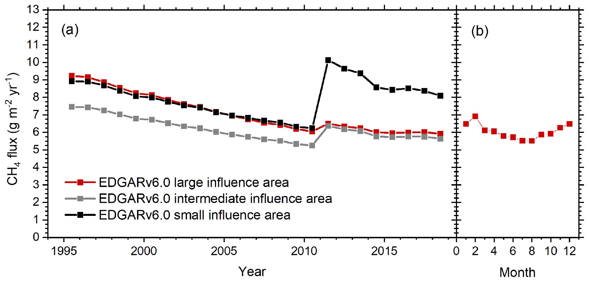
Figure 3 (a) Long-term trends of CH₄ fluxes as reported by the EDGARv6.0 emission inventory (Crippa et al., 2021). Trends for all three influence areas show a significant decrease from 1995 to 2010 of about 30 %. In 2011 an abrupt increase is observed, which is largest for the small influence area, due to an artefact of reported emissions in the MA/LU pixel (see text). (b) Seasonal cycle of 2010 emissions in the large influence area of Heidelberg.

As already mentioned in Sect. 2.1, given their predominant point-source nature, it will not be possible to provide reliable information on the total CH₄ source strengths e.g. from MA/LU with the RTM, as this method is only applicable for area sources that are similarly homogeneously distributed as those of ²²²Rn (Eq. 4). Potentially large contributions from industrial point sources to the total flux will thus be wholly or partially missing in the RTM-based TD flux estimate so that results are likely biased low. As large point-source emissions have to be reported directly to the European pollutant release and transfer (E-PRTR) register database (https://prtr.eea.europa.eu/, last access: 30 November 2021) by the facility, these bottom-up data are, however, likely much more accurate than any top-down estimate, as they are often based on direct measurements. But the more homogeneously distributed area sources dominating in the immediate neighbourhood of Heidelberg, such as energy for buildings, road transport, enteric fermentation, and de-centralised waste management, will probably be well represented in the RTM-based flux estimates. In the inventories these fluxes are associated with much larger uncertainties than those from point sources and are thus a rewarding target for the RTM.

2.3 Radon exhalation rates in the Heidelberg footprint

The most important prerequisite to apply the radon tracer method for quantitative GHGs flux estimates is representative ²²²Rn soil exhalation rates in the footprint of the station, as errors in the derived GHG fluxes will be directly proportional to errors in the ²²²Rn fluxes (see Eq. 4). The four panels on the left of Fig. 4 show the spatial distributions of ²²²Rn fluxes in the large ca. 150 km×150 km influence area of Heidelberg as estimated by Karstens et al. (2015) from bottom-up soil parameters and modelled soil moisture. The upper left panels (a and b) show the estimated ²²²Rn fluxes for January and July based on the 2006–2010 soil moisture climatology from the ERA-Interim/Land model, while the lower left panels (c and d) show the flux distributions using the GLDAS Noah soil moisture (averaged over 2006–2012) (https://doi.org/10.1594/PANGAEA.854715). Large differences are seen between the models. Along the Rhine river in the north-west of Heidelberg (black dot in the centre of each map) where a few excavated lakes are also located, we find reduced ²²²Rn fluxes compared to the areas in the immediate surroundings of Heidelberg. This flux reduction is caused by the assumption of Karstens et al. (2015) that the low water table depth close to the rivers reduces mean ²²²Rn exhalation rates. As was shown and discussed by Karstens et al. (2015), the flux estimates based on the two soil moisture models show huge differences in their absolute values over Europe. In the surroundings of Heidelberg these differences are larger than a factor of 2 throughout the year. But in both maps we see similar seasonal variations of the ²²²Rn flux, which are due to the seasonality of soil moisture with the highest values in winter and drier soils in summer and autumn. Note that in the STILT model runs discussed in Sect. 3.5 we use the average of both ²²²Rn flux maps, which we call “climatology”.

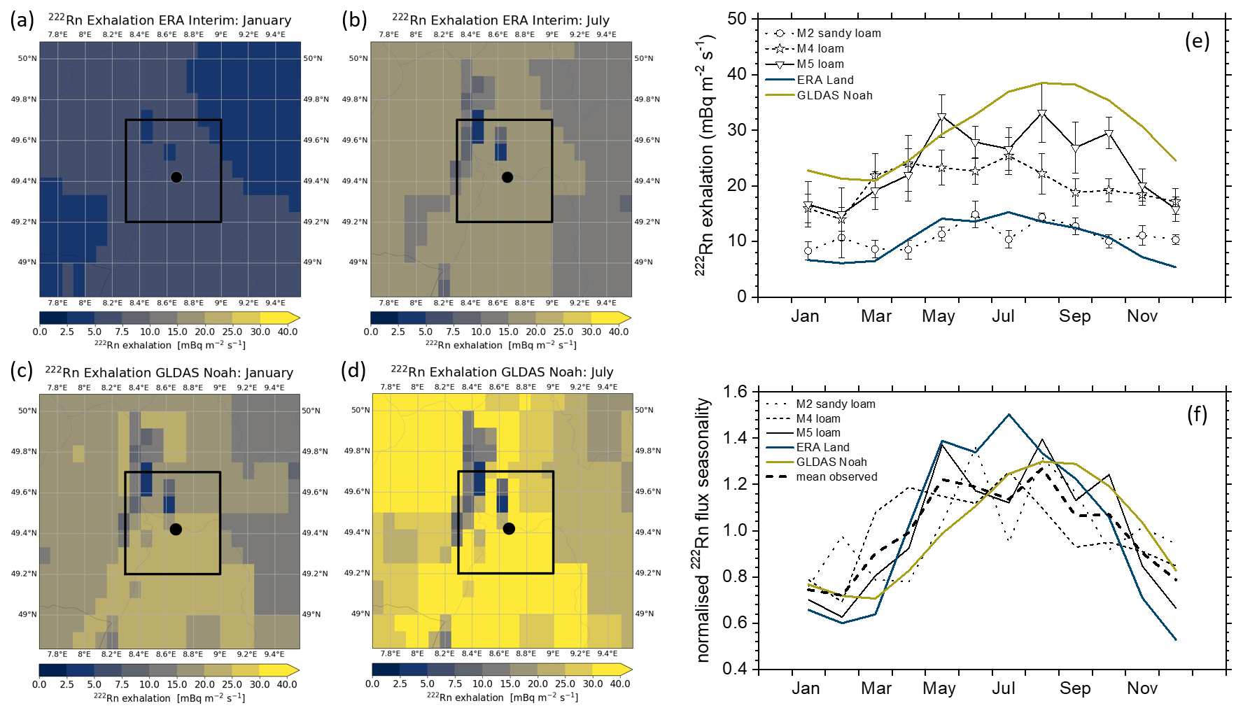
Figure 4 (a–d) ²²²Rn exhalation rates as estimated by Karstens et al. (2015) for the large Heidelberg influence area based on the ERA-Interim/Land (a, b) and GLDAS Noah (c, d) soil moisture models for January (a, c) and July (b, d). The small influence area is marked by the black rectangle with Heidelberg in its approximate centre (black dot). The very low ²²²Rn fluxes north-west of Heidelberg stem from the ²²²Rn flux limitation assumed in Karstens et al. (2015) based on the water table depth map by Miguez-Macho et al. (2008). (e) Mean seasonal cycle of the modelled fluxes in comparison to measurements conducted south of Heidelberg on sandy loam (M2) and loamy soils (M4, M5). Normalised (to their annual means) seasonal cycles of the fluxes shown in (e) are displayed in (f). The mean observed ²²²Rn flux seasonality is also shown as a thick dashed line.

In Heidelberg we are in the favourable situation that long-term observations of the ²²²Rn flux from soils have been conducted since the late 1980s (Dörr and Münnich, 1990; Schüßler, 1996). Jutzi (2001) has gathered these early data from five long-term measurement sites south of Heidelberg with different soil types to estimate mean seasonal cycles of the ²²²Rn flux. The data from three of these sites, i.e. those which have soil properties closest to the soil textures underlying the map of Karstens et al. (2015), are displayed in Fig. 4e. Measurements from the sandy soils at stations M1 and M3 have not been included as they are less representative for our footprint and showed annual mean ²²²Rn fluxes a factor of 2 smaller than at all other sites, which have been sampled in the last 10 years in the surroundings of Heidelberg (Schwingshackl, 2013). The ²²²Rn flux measurements south of Heidelberg were also used by Karstens et al. (2015), together with more recent measurements from Schmithüsen (2012) and Schwingshackl (2013) conducted north of Heidelberg to evaluate their bottom-up process-based calculations of the ²²²Rn flux for the respective pixels. They reported significant differences in ²²²Rn flux when based on the different soil moisture models, ERA-Interim/Land or GLDAS-Noah LSM, but also between models and observations (see their Figs. 6 and 7). Here we compare in Fig. 4e both model estimates for the two pixels in which the measurement sites south of Heidelberg are located with the observations from M2, M4, and M5. These measured ²²²Rn fluxes for sandy loam (M2) and loam (M4 and M5) lie between the two model estimates, with the latter covering a range of (annual) mean ²²²Rn fluxes of more than a factor of 2. Therefore, if no representative ²²²Rn flux observations are available in the footprint of a monitoring site where the RTM shall be applied, depending on the soil moisture model we chose for the ²²²Rn flux estimate, GHG emissions will differ by a factor of 2 or more. In addition, if the distribution of soil types is very heterogeneous, this will cause further uncertainty in individual RTM-based flux estimation. Based on the maps shown in Fig. 4a–d for the Heidelberg influence areas (large or small), this heterogeneity of soil textures together with water table depth flux adjustment would contribute about 15 %–30 % to the spatial variability of estimated nighttime ${\mathrm{CH}}_{\mathrm{4}}/{}^{\mathrm{222}}\mathrm{Rn}$ ratios.

On the other hand, Fig. 4e indicates that the relative seasonality is similar in the two modelled fluxes and in the observed fluxes. This seasonality of ± (25–30) % may introduce a seasonality in atmospheric ²²²Rn activity concentrations and further in the ${\mathrm{CH}}_{\mathrm{4}}/{}^{\mathrm{222}}\mathrm{Rn}$ slopes. It needs to be corrected for if the annual mean RTM-based nocturnal CH₄ emission estimates (including their potential seasonality) shall be compared with bottom-up inventories. The measured seasonality and modelled seasonality of ²²²Rn fluxes in the two pixels south of Heidelberg were therefore normalised to their respective annual means and are shown in Fig. 4f. The seasonality of the mean observed flux (dashed line in Fig. 4f) is used to normalise the ${\mathrm{CH}}_{\mathrm{4}}/{}^{\mathrm{222}}\mathrm{Rn}$ slopes of the individual nighttime correlations (Sect. 3.1). To finally estimate observation-based annual mean nocturnal CH₄ fluxes with the radon tracer method (Sect. 3.4) we will use the mean observed total flux at M2, M4, and M5 of 18.3±4.7 $\mathrm{mBq}{\mathrm{m}}^{-\mathrm{2}}{\mathrm{s}}^{-\mathrm{1}}$. The uncertainty of this observation-based mean flux represents the 1σ standard error of the mean at all three sites. To estimate the STILT-model-based nocturnal CH₄ emissions we use the mean climatological ²²²Rn flux of the small influence area, which is slightly smaller, namely 16.7±4.2 $\mathrm{mBq}{\mathrm{m}}^{-\mathrm{2}}{\mathrm{s}}^{-\mathrm{1}}$. Here the uncertainty represents the standard deviation of the individual pixels in the small influence area.

In Fig. 4 we present only monthly mean ²²²Rn fluxes and their spatial and temporal variability. However, we also expect variability of the ²²²Rn flux from day to day due to short-term soil moisture variations (Lehmann et al., 2000). In order to estimate this variability, we would need ²²²Rn flux data at higher temporal resolution. Such high-frequency data are, however, not available for the Heidelberg footprint. We therefore estimated hypothetical daily mean ²²²Rn fluxes from soil moisture data at the long-term measurement site Grenzhof, which is located about 6 km to the west of the Heidelberg monitoring station. Monthly mean soil moisture measurements from Grenzhof (2007–2008) have already been shown in Karstens et al. (2015) in their comparison with monthly mean modelled soil moisture data (see their Fig. 7d). Here we use the daily mean measurements of soil moisture and temperature in the upper 30 cm of the soil from Grenzhof (Wollschläger et al., 2009) and estimate daily mean hypothetical ²²²Rn fluxes for this site with the same methodology as used by Karstens et al. (2015). We assume a ²²²Rn source strength of the soil material of Q=27.8 $\mathrm{mBq}{\mathrm{m}}^{-\mathrm{3}}{\mathrm{s}}^{-\mathrm{1}}$, chosen such that the annual mean ²²²Rn flux for 2007 and 2008 fits the annual average observation-based flux value for the Heidelberg influence area (18.3±4.7 $\mathrm{mBq}{\mathrm{m}}^{-\mathrm{2}}{\mathrm{s}}^{-\mathrm{1}}$). Details of the calculations are given in Appendix A; the results are displayed in Fig. A1.

As expected from the soil moisture variability (Fig. A1a) the short-term changes in the hypothetical ²²²Rn flux (Fig. A1b) are smallest during December to March, when soil moisture is at its maximum and much less variable than during spring, early summer, and autumn. In these latter seasons, the day-to-day variability can reach up to ±30 %. On average the day-to-day variability of the hypothetical ²²²Rn flux at Grenzhof was estimated to ±10 % (Fig. A1c). Besides this short-term variability, we also observe a large difference of soil moisture in early summer between the two years: the rather wet June and July 2007 yield more than 30 % lower ²²²Rn fluxes than estimated for June and July 2008. Early summer and autumn precipitation and thus soil moisture can vary strongly, causing potentially huge differences in the ²²²Rn flux from year to year. These short-term and inter-annual variations of the ²²²Rn exhalation rate will contribute to the day-to-day and inter-annual variability of nighttime ${\mathrm{CH}}_{\mathrm{4}}/{}^{\mathrm{222}}\mathrm{Rn}$ ratios. They increase the uncertainty of individual (e.g. monthly) RTM flux estimates and potentially their long-term trends. Note that the dry summers of the last decade in Europe (e.g. Hanel et al., 2018) are likely associated with higher ²²²Rn fluxes, at least in summer and autumn. If not accounted for, these ²²²Rn flux variations may lead to systematic biases in RTM-based emission estimates and their long-term trends.

2.4 CH₄ measurements

Air sampling from the roof of the Institute of Environmental Physics building (INF 229) for gas chromatographic (GC) analysis was performed via two separate intake lines: one in the south-eastern corner and one in the south-western corner of the roof. These two intake lines were installed to detect potential very local contamination by GHG emissions from the air exhaust of the building or from other very nearby sources. Only during very few occasions were data manually rejected if concentrations from the two intake lines showed a major deviation. In all such cases this deviation could be attributed to a problem with the intake system. Half-hourly mean values of both intake lines were then calculated and used for further evaluation (Levin and Hammer, 2021). Data from the years 1996–1998 stem from sampling at the old IUP building (INF 366), about 500 m to the west of the new building (INF 229). Also in these early years, air was collected from the roof of the building from approximately 25 $\mathrm{m}\mathrm{a}.\mathrm{g}.\mathrm{l}.$ The GC instrumentation was the same as in INF 229.

The combined Heidelberg gas chromatographic system (Combi-GC) was designed to simultaneously measure CO₂, CH₄, N₂O, SF₆, CO, and H₂. It was optimised to measure ambient concentration levels for each trace gas with a temporal resolution of 5 min (Hammer et al., 2008). For CH₄ analysis, a HP5890II (Hewlett-Packard) GC equipped with a flame ionisation detector (FID) was used. Ambient air was dried to a dew point of ca. −35 ^∘C before analysis. Methane mole fraction is referenced to the WMO X2004A mole fraction scale (Dlugokencky et al., 2005) with a precision of about ±3 ppb for individual measurements. A linear response of the FID was assumed over the whole range of ambient CH₄ mole fractions. For details of the measurement technique, see Hammer et al. (2008). Since January 2018, a Picarro G2401 cavity ring-down spectroscopy (CRDS) gas analyser has been used for CH₄ analysis. Air for this analyser is collected from the south-eastern intake line with 1 min mean values stored and averaged to half-hourly values, following the procedures of the European ICOS atmosphere network (ICOS RI, 2020). The typical standard deviation of these half-hourly data as calculated from the 1 min data is about ±2–10 ppb, depending on ambient air variability. As for the GC, CRDS measurements are reported on the WMO X2004A mole fraction scale.

2.5 Atmospheric ²²²radon and meteorological measurements

Atmospheric ²²²Rn activity concentration is determined via its measured ²¹⁴polonium (²¹⁴Po) daughter activity using the static filter method as described by Levin et al. (2002). Based on the results from a European-wide radon comparison study, which included parallel measurements of the Heidelberg monitor with a preliminary calibrated radon detector from ANSTO (Williams and Chambers, 2016; Griffiths et al., 2016), we applied a constant ${}^{\mathrm{222}}\mathrm{Rn}{/}^{\mathrm{214}}$Po disequilibrium correction factor to the data of 1.11 and report all data on the ANSTO scale, which turned out to be another factor of 1.11 higher than the original IUP Heidelberg calibration (Schmithüsen et al., 2017). As the intake line was less than 2 m, no line loss correction (Levin et al., 2017) was applied to the data (Levin and Hammer, 2021). Depending on the ambient activity concentration level, half-hourly ²²²Rn activity concentration measurements in Heidelberg have a typical uncertainty of ±15 % (1σ), including the currently estimated uncertainty of all correction factors. The constant overall correction factor of 1.23 for the Heidelberg ²²²Rn data may, however, be subject to future changes once new calibration and intercomparison results from a metrology project (Röttger et al., 2021) become available. A possible bias in the ²²²Rn activity concentrations would also change the ${\mathrm{CH}}_{\mathrm{4}}/{}^{\mathrm{222}}\mathrm{Rn}$ slopes and therewith the RTM-based estimates of the nocturnal CH₄ flux in the Heidelberg footprint.

The wind sensors are mounted on a mast on the southern side of the institute's roof at a height of 37 $\mathrm{m}\mathrm{a}.\mathrm{g}.\mathrm{l}.$ Until 2011, wind speed was measured using a spherical cup anemometer and wind direction by a weather vane. From spring 2011 onwards, wind speed and wind direction have been measured using a 2D sonic anemometer (Thiess, Germany). For both instrument generations data were averaged to 5 min means.

3 Results

3.1 Estimating mean nighttime ${\mathrm{CH}}_{\mathrm{4}}/{}^{\mathrm{222}}\mathrm{Rn}$ ratios from half-hourly observations

For the period of 1996 to 2020 (except for 1999, when the institute moved from INF 366 to INF 229 and no CH₄ observations are available), we calculated least squares fits of the half-hourly atmospheric CH₄ and ²²²Rn observations from 21:00 to 04:00 CET the next morning. To ensure that meaningful signals are evaluated, we set a lower limit of 1.5 Bq m⁻³ for the ²²²Rn range during the correlation period, which is about half of a typical mean range during all nights. In most years more than 45 nights were left, in which the correlation coefficient (R²) of the nighttime ${\mathrm{CH}}_{\mathrm{4}}/{}^{\mathrm{222}}\mathrm{Rn}$ regressions was better than or equal to 0.7. Anthropogenic CH₄ emissions in the Heidelberg footprint have only a small seasonal variation of less than ±15 % (Crippa et al., 2021, and Fig. 3b), and there are no wetlands with temperature-dependent anaerobic CH₄ production in our region. However, as discussed in Sect. 2.3, the measured and modelled ²²²Rn exhalation rates from soils both exhibit a pronounced seasonality. In our observations and also in both model estimates the ²²²Rn flux during winter is up to 30 % lower than the annual average, and it is up to 26 % higher during late summer months (Fig. 4f). This seasonality of the ²²²Rn flux may result in a seasonality in atmospheric ²²²Rn activity concentrations and consequently also in the computed ${\mathrm{CH}}_{\mathrm{4}}/{}^{\mathrm{222}}\mathrm{Rn}$ ratios. A corresponding seasonality in CH₄ emissions is assumed to be much smaller in amplitude (Fig. 3b) and will be discussed later. In the analysis to follow, we therefore first normalised (de-seasonalised) all ratios on a monthly basis by multiplication with a corresponding factor that adjusts the ²²²Rn flux to its annual mean value. In the following we will first discuss these normalised ${\mathrm{CH}}_{\mathrm{4}}/{}^{\mathrm{222}}\mathrm{Rn}$ ratios, and only in Sect. 3.5 are RTM-based nocturnal CH₄ fluxes estimated along with their potential seasonality. This intermediate step was taken because of the large uncertainty of the absolute ²²²Rn flux in contrast to its much better-defined seasonality (see Sect. 2.3 and Fig. 4f).

All selected normalised ${\mathrm{CH}}_{\mathrm{4}}/{}^{\mathrm{222}}\mathrm{Rn}$ regression slopes with an R²≥0.7 are displayed in Fig. 5a. On average, more than 80 % of ${\mathrm{CH}}_{\mathrm{4}}/{}^{\mathrm{222}}\mathrm{Rn}$ slopes vary between about 7 and 30 ppb $(\mathrm{Bq}{\mathrm{m}}^{-\mathrm{3}}{)}^{-\mathrm{1}}$. However, we also occasionally find slopes that are much larger than 40 ppb $(\mathrm{Bq}{\mathrm{m}}^{-\mathrm{3}}{)}^{-\mathrm{1}}$. In order to evaluate how sensitive ${\mathrm{CH}}_{\mathrm{4}}/{}^{\mathrm{222}}\mathrm{Rn}$ slopes are to the selected nighttime interval chosen for the regressions, we also calculated slopes for an increased and a reduced time span, i.e. from 20:00 to 05:00 and from 22:00 to 03:00 CET. The general shape of the distributions (frequency of positive outliers) is very similar, and also the overall means differ by only ±3 %. However, differences can be more than 15 % in individual years. We also evaluated how sensitive the annual mean slopes are to the threshold of the correlation coefficient R². When selecting only the nights when R² is equal to or larger than 0.8, mean slopes are about 3 % higher than when including all slopes with an $R^{\mathrm{2}}\ge \mathrm{0.7}.$ Thus, a small bias may be introduced, depending on the choice of the nighttime regression interval and also depending on the requested goodness of correlation between CH₄ and ²²²Rn. It is also important to note that the number of nights with R²≥0.7 increases systematically with the length of the tested regression time periods. The RTM is based on the co-variation of trace gases and ²²²Rn through changing atmospheric mixing. Since there is no causal correlation between the emission processes of the two gases, their different spatial source heterogeneity in combination with changing footprints leads to a reduced number of valid correlations with a shorter observation period. In contrast, more extended regression periods with variable footprints increase the probability of averaging across spatial heterogeneity of emissions.

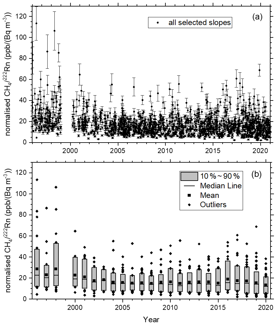
Figure 5 (a) Individual normalised ${\mathrm{CH}}_{\mathrm{4}}/{}^{\mathrm{222}}\mathrm{Rn}$ slopes and their 1σ uncertainties of linear regressions with R²≥0.7, calculated from half-hourly nighttime (21:00 to 04:00 CET) data. (b) Annually aggregated ${\mathrm{CH}}_{\mathrm{4}}/{}^{\mathrm{222}}\mathrm{Rn}$ slopes presented as box plots with the boxes including 80 % of the data.

Interestingly, mean slopes are only about 3 % different (larger) if only values obtained for situations when both concentrations increase are included compared to when we also include the approximately 20 % of situations when both gases show a positively correlated decrease between the start and the end of the regression interval. This finding may be a special characteristic of our sampling site, where the air intake is only at 30 $\mathrm{m}\mathrm{a}.\mathrm{g}.\mathrm{l}.$ During very stable situations and calm winds the air intake can obviously be either below or above the local surface inversion (if this is around 30 m), which results in very abrupt but synchronous changes in both gases during some nights. As mentioned in Sect. 2.1 we can describe this as a case in which two air mass components, i.e. one enriched by emissions from ground-level sources with a well-defined ${\mathrm{CH}}_{\mathrm{4}}/{}^{\mathrm{222}}\mathrm{Rn}$ ratio and another cleaner component from the residual layer that has a ${\mathrm{CH}}_{\mathrm{4}}/{}^{\mathrm{222}}\mathrm{Rn}$ ratio similar to that during well-mixed situations the afternoon before. These two components are mixed at various ratios. In such a situation all measured ${\mathrm{CH}}_{\mathrm{4}}/{}^{\mathrm{222}}\mathrm{Rn}$ ratios lie on one mixing line, which corresponds to the regression line in our approach. With this picture in mind, it becomes immediately clear that in Eqs. (1) and (2) (Sect. 2.1), besides the concentrations of CH₄ and ²²²Rn, the mixing height H(t) may also vary temporally and does not need to be constant during a single night to apply the nocturnal accumulation RTM. We thus kept all nights when CH₄ and ²²²Rn are well correlated and with a positive slope for calculating annual means and further evaluating the slopes.

3.2 Relating ${\mathrm{CH}}_{\mathrm{4}}/{}^{\mathrm{222}}\mathrm{Rn}$ slopes to footprints

The ${\mathrm{CH}}_{\mathrm{4}}/{}^{\mathrm{222}}\mathrm{Rn}$ slopes displayed in Fig. 5 show large variability. It is of interest to explore if this variability can be explained by spatial variations in the CH₄ emissions and, if so, the extent to which we can associate the high-slope cases with hotspot emission areas in the footprint of Heidelberg. We therefore evaluated the air mass footprint based on local wind data for all nights when we obtained good (R²≥0.7) correlation between CH₄ and ²²²Rn. Let us assume that the ²²²Rn flux is spatially homogeneous; then we would expect higher slopes if the air mass has passed over the north-westerly or westerly sectors where the large CH₄ emitters from MA/LU are located (Fig. 1b). Figure 6 shows in the first column (a–c) polar plots of wind direction (angle) and speed (radius axis) with the value of the corresponding slopes colour-coded (i.e. larger slopes plotted in darker red colours). Note that we use the original 5 min mean values of wind speed and direction, together with the mean slope during the entire night (7 h). Each polar plot shows the distribution for all selected nights of the entire year (2016, 2017, and 2018 as typical examples from the later years of our record); the colour-coded segments represent annual mean values of all slopes for which a 5 min value fell into the respective wind rose segment. The second column of Fig. 6d–f shows the frequency distribution of the wind during all selected nights, while the third column (g–i) shows the distribution during all nights in the respective year (21:00–04:00 CET).

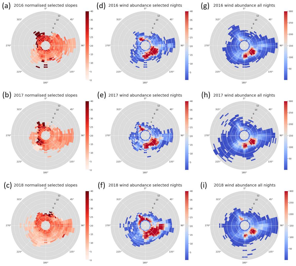
Figure 6 (a–c) Distribution of nighttime slopes (in $\mathrm{ppb}\left(\mathrm{Bq}{\mathrm{m}}^{-\mathrm{3}}{)}^{-\mathrm{1}}\right)$ by local wind direction (^∘) and velocity (m s⁻¹) for the years 2016, 2017, and 2018. The corresponding frequency distributions of wind direction and velocity for the selected nights are displayed in (d–f), while the distributions for all nights of the respective year (from 21:00–04:00 CET) are shown in (g–i). It is clearly visible that wind velocities are generally lower during the selected nights than during all nights.

The frequency distributions of 2016 and 2017 indeed show higher average slopes when the wind comes from north-westerly directions, but in 2018 high slopes are also associated with the northern or north-eastern wind direction. Interestingly, the easterly and south-easterly sectors show average slopes that are often smaller than about 20 ppb $(\mathrm{Bq}{\mathrm{m}}^{-\mathrm{3}}{)}^{-\mathrm{1}}$. This is a wind sector where EDGARv6.0 also generally reports lower than average emissions (Fig. 1b). A problem with this analysis is that during low wind speed, the wind direction is not well defined and may change by (more than) 180^∘ within a single night. The measured air would then be influenced by emissions from various sectors with different CH₄ emissions. This could smooth out an otherwise clear association of slopes with certain wind sectors. Also, low wind speed situations are more frequent during stable nights (as indicated for the selected nights in Fig. 6d–f) with a shallow boundary layer and large nocturnal increases in CH₄ and ²²²Rn, i.e. nights with good correlation between the two gases and when the nocturnal accumulation RTM can be principally applied. We should also keep in mind that some of the high emissions in the MA/LU hotspot area are probably from point sources that may not be fully captured by the RTM. Also the frequency distribution of wind directions generally (for all nights) favours more southerly and south-easterly winds, which reduces the likelihood to monitor the high CH₄ emissions from the MA/LU area. Nevertheless, we can roughly separate influence areas, which, on an annual mean basis, differ in their mean slopes by more than a factor of 2. This indicates that a large share of the variability of slopes (Fig. 5) is caused by the heterogeneity of CH₄ emissions around Heidelberg.

3.3 The influence of ²²²Rn flux variability on the variability of ${\mathrm{CH}}_{\mathrm{4}}/{}^{\mathrm{222}}\mathrm{Rn}$ slopes

Besides the heterogeneous distribution of CH₄ emissions in the Heidelberg footprint, we expect part of the variability in the ${\mathrm{CH}}_{\mathrm{4}}/{}^{\mathrm{222}}\mathrm{Rn}$ slopes to also be due to variations of the spatial distribution of the ²²²Rn exhalation rate. Figure 4a–d show the spatial ²²²Rn flux distributions for the large Heidelberg influence area in January and July for both soil moisture models. Although mean fluxes from the two different soil moisture models differ by more than a factor of 2, the spatial variability within one map varies by only ± (15–25) % within the large area and slightly more in the small 70 km×70 km influence area. Therefore, the spatial variability of the ²²²Rn flux probably contributes much less to the variability of slopes than that of the CH₄ flux (see also Sect. 3.5 where we investigate the contributions of CH₄ vs. ²²²Rn flux heterogeneity to modelled ${\mathrm{CH}}_{\mathrm{4}}/{}^{\mathrm{222}}\mathrm{Rn}$ slopes). Also, the short-term day-to-day variability of the estimated “hypothetical” ²²²Rn flux, as elaborated in Appendix A and displayed in Fig. A1c for the years 2007 and 2008, may contribute to the variability of slopes. The hypothetical daily flux estimates, which are based on the measured daily mean soil moisture values, show a mean day-to-day variability of ±10 %, but during early summer 2007 and likely also in other years, particularly during spring and autumn, short-term deviations from monthly mean fluxes can be as large as 30 %. However, these deviations are still too small to explain a major share of the observed slope variability displayed in Fig. 5.

3.4 Estimating CH₄ fluxes with the RTM and comparison with EDGARv6.0 emission trends and seasonality

As shown in the previous section, the spatial variability of CH₄ emissions and, to some extent, also the spatial and temporal variations of the ²²²Rn flux in the influence area of Heidelberg are large and make reliable estimates of RTM-based CH₄ emissions from selected sectors (e.g. of industrial processes in MA/LU) or for individual short periods highly uncertain. But we can estimate average nocturnal CH₄ emissions from the footprint of the station. As a first attempt to apply the nocturnal accumulation RTM we use the observation-based ²²²Rn flux, which was estimated as the mean of our measurements at M2, M4, and M5 to be 18.3±4.7 $\mathrm{mBq}{\mathrm{m}}^{-\mathrm{2}}{\mathrm{s}}^{-\mathrm{1}}$ (Sect. 2.3). The corresponding calculated CH₄ flux is plotted as a black histogram in Fig. 7. The uncertainty of the absolute RTM-based CH₄ fluxes is dominated by the uncertainty of the mean ²²²Rn flux and is exemplarily plotted as black error bars for the first and last year of observations. A significant decrease in emissions by about 30 % is observed from 1995 until about 2004. This decrease is in agreement with the trend of bottom-up EDGARv6.0 emissions from 1995–2010 calculated for all three influence areas in Fig. 3a. However, while EDGARv6.0 emissions show a further decrease after 2004, our RTM-based estimates are more or less constant after 2004, showing an inter-annual variability of less than ±10 %.

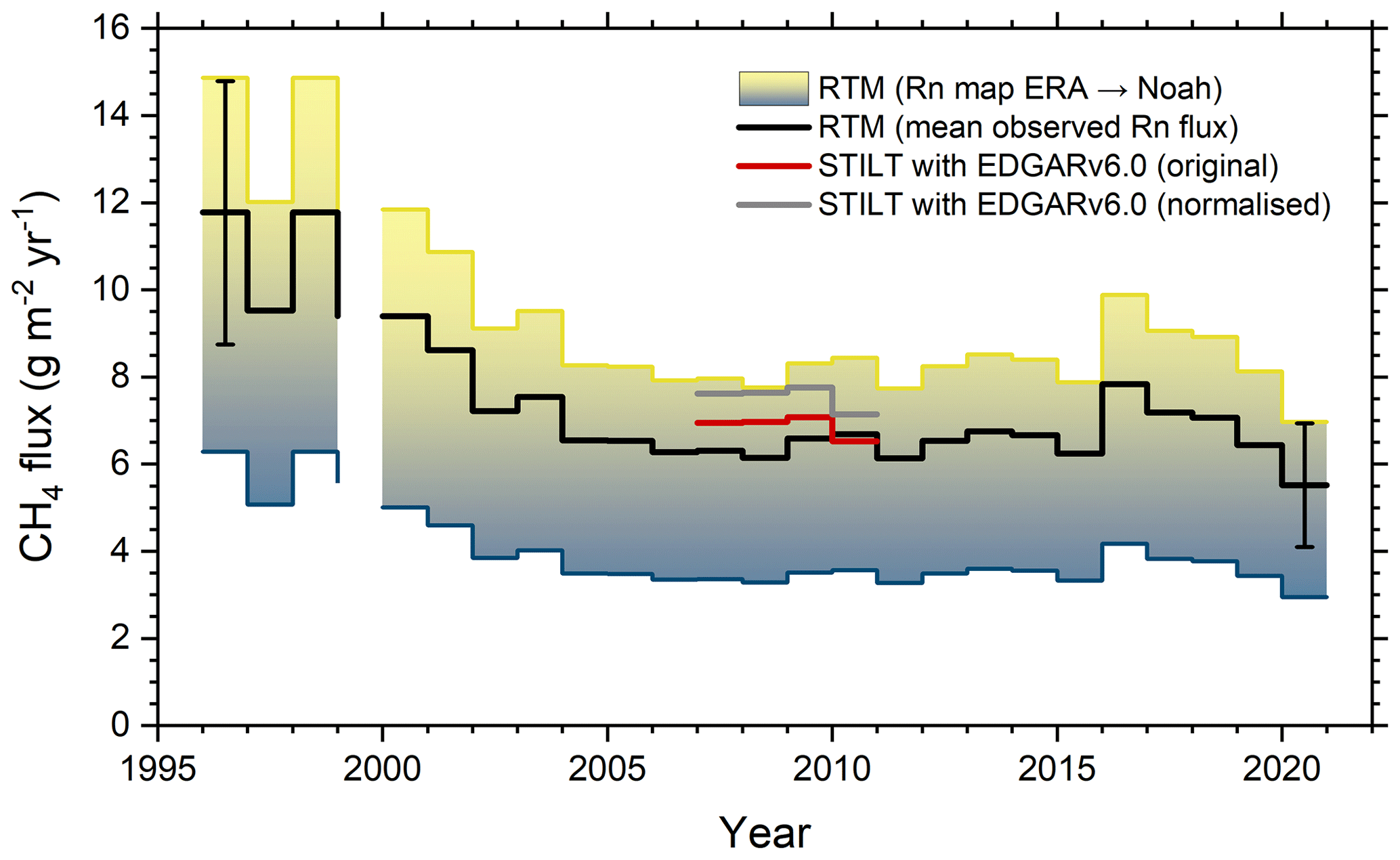
Figure 7 Long-term trend of the RTM-based CH₄ flux in the Heidelberg footprint. The black histogram (with typical RTM-based uncertainties shown for the first and the last year of observations) was calculated based on the observation-based ²²²Rn flux of 18.3±4.7 $\mathrm{Bq}{\mathrm{m}}^{-\mathrm{2}}{\mathrm{s}}^{-\mathrm{1}}$. The coloured area shows the range of RTM-based CH₄ flux estimates if either the GLDAS Noah soil moisture (yellow) or the ERA-Interim/Land soil moisture (blue) ²²²Rn flux average of the small influence area had been used to calculate RTM-based CH₄ fluxes. Also included in the diagram are RTM-based results from STILT-modelled CH₄ and ²²²Rn data for 2007–2010 (based on the slopes in Fig. 8a). The red line shows the original results using the EDGARv6.0 emission inventory and the ²²²Rn flux climatology, while the grey line shows the STILT results normalised to the observation-based ²²²Rn flux (see text).

In Fig. 7 we also include the range of CH₄ emissions we would estimate when using the mean ²²²Rn flux from the maps by Karstens et al. (2015). For this estimate we used the mean ²²²Rn fluxes from the small influence area. As expected from the huge difference in ²²²Rn fluxes between the two soil moisture models (Fig. 4e), possible RTM-based CH₄ emission estimates would cover a range of more than a factor of 2 (indicated in Fig. 7 by the coloured area). Using the mean ²²²Rn flux from both model estimates, i.e. the climatology, would – accidentally – yield a similar (ca. 10 % lower) RTM-based CH₄ flux as when using the observation-based ²²²Rn flux for the Heidelberg footprint.

The EDGARv6.0 inventory reports a small seasonal cycle of CH₄ emissions for the Heidelberg influence areas as displayed in Fig. 3b for the large influence area. Due to the large day-to-day variability of slopes (Fig. 5a), visual inspection does not suggest a very regular seasonal variation. However, when grouping slopes into monthly bins and calculating from these monthly values a mean seasonal cycle for the period when annual mean RTM-based emissions were almost constant (i.e. from 2004–2015), we observe on average slightly higher ${\mathrm{CH}}_{\mathrm{4}}/{}^{\mathrm{222}}\mathrm{Rn}$ ratios during the winter than during the summer months. This seasonality, although very variable from year to year, is in accordance with the EDGARv6.0 seasonal cycle of CH₄ emissions and therewith does not contradict but rather confirms the bottom-up estimates of the seasonality in our influence area,

3.5 Comparing the observation-based RTM results with the RTM application to preliminary STILT CH₄ and ²²²Rn simulations

One important shortcoming of RTM-based GHG flux estimates is the lack of information on the actual influence area for which the estimated flux is representative. In Sect. 2.2 and Fig. 2 we could only roughly localise the large ca. 150 km×150 km influence area for Heidelberg contributing most of the source influence to the nighttime concentration changes within the 7 h used for the RTM-based flux estimates. Quantitative comparison with bottom-up emission inventories, however, requires actual weighting of the influence area, in particular if the distribution of the GHG emissions is as heterogeneous as in the Heidelberg surroundings. This weighting can be achieved with regional transport model simulations. For the following STILT model estimates the footprints were mapped on a $\mathrm{1}/\mathrm{12}{}^{\circ }\text{latitude}\times \mathrm{1}/\mathrm{8}{}^{\circ }$ longitude grid and were coupled (offline) to the EDGARv6.0 emission inventory (Crippa et al., 2021) for CH₄ concentration estimation, neglecting seasonality of emissions. We also simulated atmospheric ²²²Rn activity concentrations based on the two ²²²Rn flux maps of Karstens et al. (2015) (the average climatology of ERA-Interim/Land and Noah GLDAS was used for the simulations). The modelled regional concentration components represent only the influence from surface fluxes inside the model domain (covering the greater part of Europe, i.e. an area much larger than the large influence area defined in Sect. 2.2). The background concentrations for CH₄ and ²²²Rn outside our modelling domain have been neglected as we are only interested in nighttime changes in both trace gases. We then also applied the RTM to these preliminary model results and compared the slopes and their typical distribution to those from the observations. Comparing modelled with observed slopes rather than absolute concentrations has the advantage that incorrect parameterisation of the nighttime boundary layer height by the model partly cancels, while the relative footprint area weighting may still be reliable, even for nighttime simulations.

Figure 8 shows the normalised observed and modelled ${\mathrm{CH}}_{\mathrm{4}}/{}^{\mathrm{222}}\mathrm{Rn}$ slopes in Heidelberg for the years 2007–2010 and their distributions. We also ran the STILT model for 2011, but due to the error in the EDGARv6.0 emissions from 2011 onwards, we used the results only as a sensitivity test (see below). Although we use the same selection criteria for the modelled concentration regressions as for the observations, the number of nights with good correlations of CH₄ and ²²²Rn is about 5 times higher than for the observations. Note that we do not want to compare modelled with observed slopes of individual nights, e.g. in a scatter plot, because we are mainly interested in comparing mean values (to further translate them into mean emission rates as displayed in Fig. 7) and their distributions (Fig. 8b). In the model-based slopes we find a number of very high values, which we do not see in 2007–2010 in the observed slopes. We can clearly identify these high modelled slopes as being associated with north-westerly winds and thus as a strong influence from hotspot CH₄ emissions in these situations. Although the hotspots in reality probably have very localised emissions and are not captured by the nocturnal accumulation RTM in the real world, in the model these emissions are distributed over the area of the entire approximately 10 km×10 km wide pixel so that during stable winds good correlations between ²²²Rn and CH₄ may occur over an entire night, and very high ${\mathrm{CH}}_{\mathrm{4}}/{}^{\mathrm{222}}\mathrm{Rn}$ ratios can be obtained. This finding is confirmed by STILT model results for the year 2011, in which CH₄ emissions in EDGARv6.0 are more than doubled in the MA/LU pixel. In this year we find a larger number of high slopes than in the years 2007–2010, some of them exceeding 100 ppb $(\mathrm{Bq}{\mathrm{m}}^{-\mathrm{3}}{)}^{-\mathrm{1}}$.

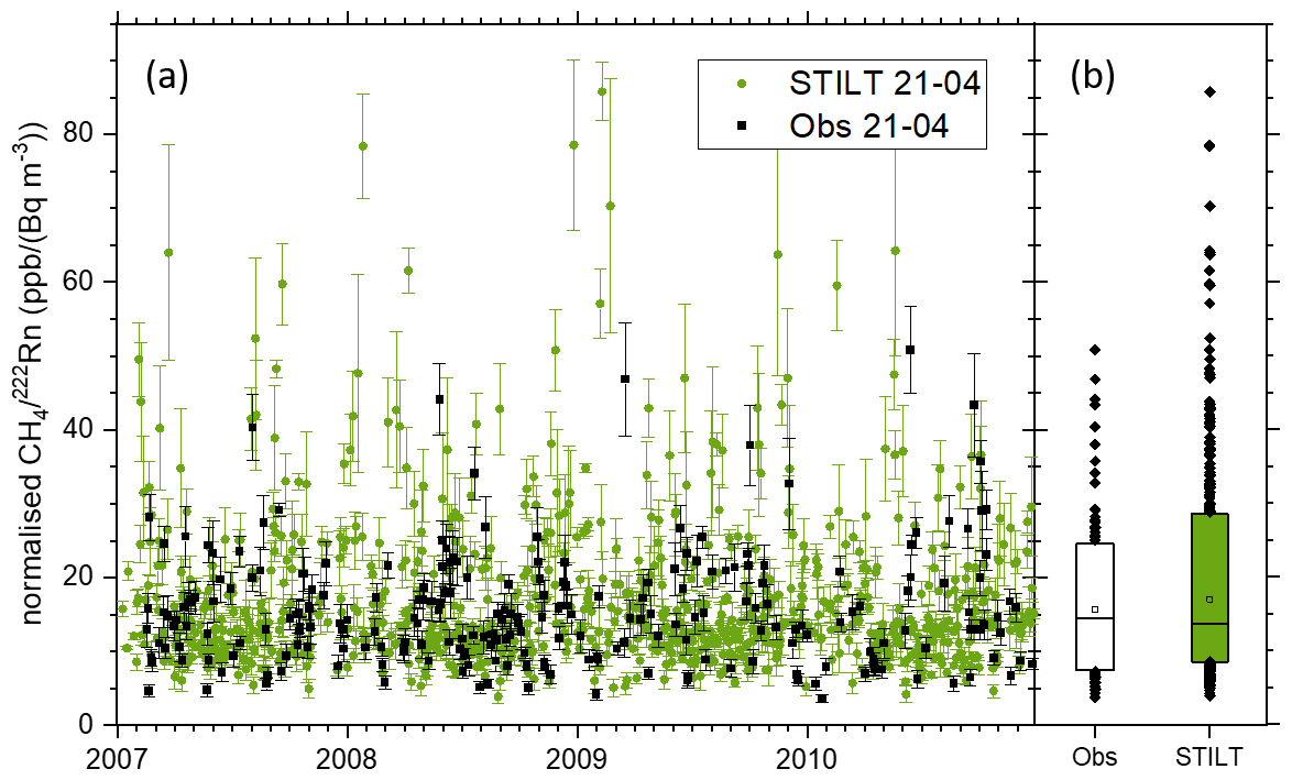
Figure 8 (a) Variability of observed (Obs, black squares) and simulated (STILT, green dots) nighttime ${\mathrm{CH}}_{\mathrm{4}}/{}^{\mathrm{222}}\mathrm{Rn}$ slopes from 2007 to 2010. (b) The distributions of all slopes with the boxes including 80 % of the data, the open squares representing the mean, and the horizontal lines the median values. Note that for the further discussion we excluded the three modelled values >70 ppb $(\mathrm{Bq}{\mathrm{m}}^{-\mathrm{3}}{)}^{-\mathrm{1}}$.

If we exclude the three outliers above 70 ppb $(\mathrm{Bq}{\mathrm{m}}^{-\mathrm{3}}{)}^{-\mathrm{1}}$ in 2008 and 2009 in the averaging of the modelled slopes, we obtain rather good agreement with the mean observed slopes (i.e. observations $=(\mathrm{15.6}\pm \mathrm{7.9})\mathrm{ppb}(\mathrm{Bq}{\mathrm{m}}^{-\mathrm{3}}{)}^{-\mathrm{1}}$; model $=(\mathrm{16.7}\pm \mathrm{8.5})\mathrm{ppb}(\mathrm{Bq}{\mathrm{m}}^{-\mathrm{3}}{)}^{-\mathrm{1}})$. Also, the relative variability is then very similar in the modelled compared to the observed slopes, i.e. 50 % vs. 52 % (Fig. 8b). This justifies quantitative comparison between model results and observations. However, even under the assumption that the modelled footprint area is correct, we are still not able to quantitatively validate EDGARv6.0 emission estimates through comparison between the model and observations as long as we do not know the true ²²²Rn flux in this footprint area. But we can go one step further and normalise the model results to the same ²²²Rn flux that we believe is the best estimate for the Heidelberg influence area based on observations. The model simulations were based on the ²²²Rn flux climatology of Karstens et al. (2015), which give an annual mean flux averaged over the small influence area of 16.7±4.2 $\mathrm{mBq}{\mathrm{m}}^{-\mathrm{2}}{\mathrm{s}}^{-\mathrm{1}}$ (see Sect. 2.3; the mean flux in the large influence area would be 2.5 % lower). Normalisation then increases the mean modelled slopes by a factor of $\mathrm{18.3}/\mathrm{16.7}$, leading to an overestimation of the modelled slopes compared to the observations by a factor of model $/$ observation $=\mathrm{16.7}\times \mathrm{18.3}/\mathrm{16.7}/\mathrm{15.6}=\mathrm{1.17}$. The uncertainty of this result would be about 25 %, i.e. essentially the estimated uncertainty of the mean observation-based ²²²Rn flux. Within this uncertainty we could come to the conclusion that EDGARv6.0 emissions in the Heidelberg footprint area would be slightly overestimated by (17±25) %. However, we must not forget that the observation-based RTM results (and, to some extent, also the STILT-based results) are biased low because we do not (or only partly) catch emissions from very localised CH₄ sources. How big the respective biases are is hard to quantify; it would require a dedicated sensitivity study with a realistic very high-resolution transport model and an emission inventory that separates area and point-source emissions.

We further used STILT model simulation experiments to investigate the sole influence of (1) CH₄ flux heterogeneity, (2) ²²²Rn flux heterogeneity, and (3) neglecting radioactive decay of ²²²Rn in the calculation of ${\mathrm{CH}}_{\mathrm{4}}/{}^{\mathrm{222}}\mathrm{Rn}$ slopes in Heidelberg. For these experiments we compared the standard model results with those for which we used (1) a constant CH₄ source distribution, (2) a constant ²²²Rn flux, and (3) treated ²²²Rn as a stable tracer. Experiments (1) and (2) confirmed that most of the variability of ${\mathrm{CH}}_{\mathrm{4}}/{}^{\mathrm{222}}\mathrm{Rn}$ slopes in Heidelberg is due to the heterogeneity of the CH₄ source distribution. Keeping ²²²Rn fluxes constant had no significant influence on the standard deviation of the ${\mathrm{CH}}_{\mathrm{4}}/{}^{\mathrm{222}}\mathrm{Rn}$ slopes; however, spatially homogeneous CH₄ emissions reduced the variability of the slopes from about 50 % to less than 20 %. When treating ²²²Rn as a stable tracer in the model, mean slopes were 7 % lower than in the run which included radioactive decay in the modelled ²²²Rn activity concentration. This means that both modelled and observed slopes need to be corrected downwards by 7 %. This, however, has no influence on our finding that EDGARv6.0 emissions in the Heidelberg footprint may be (17±25) % too high.

4 Discussion

4.1 How reliable can RTM-based GHG flux estimates be?

The radon tracer method is a purely observation-based method to estimate nighttime fluxes from homogeneously distributed ground-level sources of trace gases. Its application is simple; in principle, it does not require sophisticated atmospheric transport modelling. Depending on the height above ground level of co-located ²²²Rn and trace gas observations, nocturnal accumulation RTM-estimated fluxes can be representative for an area of several hundred square kilometres. However, the exact area for which the estimated mean nighttime flux is representative must be estimated separately, e.g. by footprint modelling. The accuracy of the RTM-based trace gas flux estimates is almost solely determined by the exact knowledge of the ²²²Rn exhalation rate from the soils in the influence area of the atmospheric station. Still, even if the absolute ²²²Rn exhalation rate is not well known, and with that the absolute trace gas flux, the RTM can provide validation of long-term trace gas emission trends, for example, of GHG emission reductions. This, however, requires that the ²²²Rn flux does not show a systematic long-term trend, which, for example, may be caused by long-term changes in soil moisture in the footprint of the measurement site. Also, the mean footprint should not show a systematic trend, e.g. due to climate-driven changes in local transport patterns. This is particularly important if ²²²Rn and/or trace gas emissions show large spatial heterogeneity in the footprint.

The RTM-based CH₄ emission trend calculated from Heidelberg observations is in good agreement with the trend of the EDGARv6.0 bottom-up inventory data, and the observed seasonal cycle of CH₄ emissions also agrees, within uncertainties, with that reported for the footprint of our station. However, after 2004 mean observation-based fluxes do not show a further decrease, contrary to the values reported by EDGARv6.0. Comparison of absolute emissions is, however, difficult as point-source emissions are not fully captured by the RTM; therefore, our RTM-based fluxes are biased low. As we rely on modelled footprints for a quantitative comparison of RTM-based top-down fluxes with inventory-based bottom-up emission estimates, how reliably we can compare observed with modelled slopes will depend on the share of point-source emissions. Due to the coarse grid of the STILT model we used in this study and the coarse resolution of the inventory, point-source emissions were distributed over 10 km×10 km grid areas. This resulted in a larger number of high slopes in the model results compared to observations if the air mass came from the MA/LU hotspot emissions area. Modelling CH₄ and ²²²Rn with a higher resolution model and emission inventory could improve comparability of model results and observations, therewith helping to quantify the bias in observation-based RTM results caused by point-source emissions in a particular setting.

Large potential biases in observation- and model-based RTM flux estimates are introduced by the uncertainty of the ²²²Rn flux in the footprint. For the Heidelberg footprint, the uncertainty of 25 % for the mean ²²²Rn flux is probably an upper limit because soil texture and ²²⁶Ra content of the soils in the footprint of our station show only small variability (<10 %) (Schwingshackl, 2013; Karstens et al., 2015). But we would need more systematic and representative ²²²Rn flux observations, also at larger distances from Heidelberg, to estimate a more accurate mean observation-based flux with a smaller uncertainty range.

On the other hand, we want to emphasise that comparing simulated mean nighttime ${\mathrm{CH}}_{\mathrm{4}}/{}^{\mathrm{222}}\mathrm{Rn}$ slopes with observed slopes could be a more accurate method to evaluate bottom-up emissions than directly comparing simulated and observed nighttime CH₄ concentrations or using model inversions of nighttime data to optimise CH₄ fluxes. This problem is certainly less serious if only daytime observations are used in the inversions. However, the approximately 5-fold larger surface influences (sensitivity) during night than during day (Fig. 2c and d) may help improve top-down results. The normalisation of modelled nighttime CH₄ with modelled ²²²Rn largely eliminates errors in model transport, such as deficiencies in the parameterisation of the nocturnal boundary layer height (e.g. Gerbig et al. 2008), but in this approach the final outcome and its significance also depend on the correctness of the underlying ²²²Rn exhalation rate. This exhalation rate can easily have larger uncertainties than the GHG emission inventory we target to evaluate. For example, for Europe, different bottom-up CH₄ emission inventories agree to within 10 % or better (e.g. Petrescu et al., 2021). It is still likely that the uncertainty of BU GHG fluxes in a smaller area, which have been disaggregated from national totals and thus depend on generalised assumptions about emission factors and proxies for the different sectors, is much larger than 10 % or may even have flaws (see Sect. 2.2 and Fig. 3a).

It should perhaps also be noted that our Heidelberg site may be a special case with advantages and disadvantages to apply the nocturnal accumulation RTM. First, we have conducted the long-term observations with the same instrumentation, except for CH₄, in the last 3 years. More importantly, the air intake at about 30 $\mathrm{m}\mathrm{a}.\mathrm{g}.\mathrm{l}.$ may be favourable for RTM applications, as it frequently lies in the nocturnal surface layer, which implies that we observe sufficiently large nighttime increases in both gases to obtain good correlations. Nevertheless, at this height above ground we monitor a footprint that is large enough to not only be influenced by very local emissions. A major advantage for estimating potentially accurate CH₄ fluxes were long-term observations of the ²²²Rn exhalation rate and its seasonality from typical soil types around the station. This made the results presented here fully independent from modelled soil-moisture-based ²²²Rn flux estimation. If we had to solely rely on modelled ²²²Rn fluxes, e.g. from Karstens et al. (2015), the uncertainty range of RTM-based estimates would have been as large as a factor of 2 (Fig. 7, coloured area). The largest disadvantage of our setting is, however, that CH₄ emissions in our footprint are very heterogeneous and contain point-source emissions, which cannot be evaluated with the RTM. Therefore, observation-based but also STILT-based CH₄ flux estimates are biased low to a currently unquantifiable extent. Another point that needs to be considered is that the nocturnal accumulation RTM only estimates nighttime emissions. This may introduce another bias towards values that are too low if not compared to nighttime emissions from inventories because most anthropogenic CH₄ emissions are lower during night than during the day (Kuenen et al., 2021).

There are a number of other issues that need to be kept in mind when applying the RTM: it is important to carefully evaluate what the most appropriate nighttime period is to calculate representative trace gas fluxes. We investigated this parameter for Heidelberg and found on average about 3 % smaller CH₄ fluxes when extending the regression period from 7 to 9 h and 3 % higher fluxes when reducing it to 5 h. But for individual years mean slopes showed differences larger than 10 % when changing the length of the regression period. Also, in these scenarios the number of nights with good correlation (i.e. R²≥0.7) decreased significantly when the correlation period was shortened to 5 h or even less. The heterogeneity of CH₄ emissions in the Heidelberg footprint may have contributed to this effect, as we often have very variable wind directions during stable nights, and changes in the ${\mathrm{CH}}_{\mathrm{4}}/{}^{\mathrm{222}}\mathrm{Rn}$ slopes may lead to bad correlations if only a smaller number of data points are correlated. Also, increasing the quality of the regression from R²≥0.7 to R²≥0.8 led to an increase in the mean slope (here by 3 % on average). As the average correlation coefficient did not change when changing the regression period and selecting only nights with R²≥0.7, we finally decided to fix this period to the 7 h which during winter and summer always fall into dark nighttime (i.e. 21:00–04:00 CET). However, we have to admit that this decision was made in a rather subjective way.

4.2 Would reliable RTM-based GHG flux estimates be possible at ICOS stations?

At many stations in the ICOS atmosphere network continuous ²²²Rn observations are conducted; however, almost no systematic ²²²Rn flux observations exist in the footprint of these stations. This is a serious deficiency if the RTM shall be routinely applied in this network for top-down GHG flux estimation. Even if these measurements may be introduced in the future, they need to be conducted for a number of representative soils in the influence area and over a longer time period. We have shown that the day-to-day variability of the ²²²Rn exhalation rate can be large (Fig. A1c). Also, inter-annual variations of soil moisture due to variations in seasonal precipitation dictate a need for systematic long-term ²²²Rn flux measurements to allow for representative estimates of the mean flux and its typical seasonality. A second problem to reliably apply the nocturnal accumulation RTM at ICOS stations may be the relatively high air intake for ²²²Rn (generally >100 $\mathrm{m}\mathrm{a}.\mathrm{g}.\mathrm{l}.$). Nighttime increases in soil-borne trace gases are much smaller at these heights than at 30 m, and the layer with the air intake may be decoupled from ground-level emissions. This increases the footprint of the station with potentially more heterogeneous and possibly less well-defined ²²²Rn fluxes.

However, we could show in our study that the long-term trends of RTM- and inventory-based emission estimates did not significantly deviate from each other. Monitoring potential trends of GHG fluxes is an important task of ICOS and could very well contribute to the regular stock taking under the UNFCCC accord (UNFCCC, 2015), providing independent validation of reported trends. Still, this would require confidence that ²²²Rn fluxes have not changed over the monitoring period.

4.3 Could a better ²²²Rn flux map help to improve RTM-based GHG flux estimates?

As is shown in Fig. 4, the current ²²²Rn flux maps from Karstens et al. (2015) show huge differences depending on the soil moisture model that was used. In the case of Heidelberg, a simple averaging of these two model estimates (what we called climatology) would have fit the observations rather well (the average ²²²Rn flux for the Heidelberg influence area would then be between 16.3 and 16.7 $\mathrm{mBq}{\mathrm{m}}^{-\mathrm{2}}{\mathrm{s}}^{-\mathrm{1}}$ compared to the observation-based flux of 18.3±4.7 $\mathrm{mBq}{\mathrm{m}}^{-\mathrm{2}}{\mathrm{s}}^{-\mathrm{1}}$). Averaging both estimates would thus have been a tempting solution for the Heidelberg footprint if no observations had been available. But would averaging both maps also yield reliable estimates of the ²²²Rn flux at other sites in Europe? As was shown by Karstens et al. (2015), it is not obvious that one or the other soil moisture model or the average of both models would fit observed ²²²Rn fluxes best. There is some indication that the ERA-Interim/Land-based fluxes are generally underestimating observations (Karstens et al., 2015, Fig. 8). Today, improved so-called third-generation land reanalysis models are available (see Li et al., 2020, for an overview). Soil moisture estimates from these third-generation models have been compared to observations, and it turned out that “the European Centre for Medium-Range Weather Forecasts ERA5 model (Hersbach et al., 2018) shows higher skills than the other four products and a significant improvement over its predecessor” (Li et al., 2020). However, although the ERA5 results give realistic variability, they often show systematically higher soil moisture than the observations. In order to use these new reanalysis data, which have the advantage that they are available now at much higher temporal and spatial resolution, a method needs to be developed to scale them to precise and representative observations, which is a challenging task if based on the currently available soil moisture measurements. Only then will we be able to apply these model results in a process-based approach to calculate realistic high-resolution ²²²Rn fluxes for Europe that compare well with observations, also in their absolute values. This task is part of the European EMPIR project traceRadon (Röttger et al., 2021), which will also conduct dedicated campaigns of quasi-continuous ²²²Rn flux and soil moisture measurements. With this objective, it also has the potential to deliver a much more detailed data set to validate the new map and increase the observational basis at ICOS stations to apply the radon tracer method in the future.

5 Conclusions

The radon tracer method provides a useful observation-based top-down tool to evaluate bottom-up inventories of greenhouse and other trace gas fluxes with a homogeneous source distribution similar to that of ²²²Rn. Applying the RTM for quantitative flux estimation relies critically on the accuracy of the ²²²Rn flux in the footprint of the station. Its application for CH₄ at the Heidelberg measurement station had serious limitations due to the large heterogeneity of emissions in the influence area, which caused a huge variability of ${\mathrm{CH}}_{\mathrm{4}}/{}^{\mathrm{222}}\mathrm{Rn}$ ratios. Large point-source emissions were not captured by the RTM, thus underestimating the total flux. Results of GHG flux estimates further depend on the parameters used to apply the RTM, such as the nighttime period chosen and the requested quality of the regression (R²). Only slightly changing these parameters, e.g. extending or reducing the nighttime regression period by 2 h or choosing an R² cut-off value of 0.8 rather than 0.7, introduces systematic differences of several percent each. Quantitative comparison of RTM-based with bottom-up emission data is not directly possible without reliable footprint modelling of the nighttime observations. This may be hampered by the reliability of nighttime model transport, but also applying the RTM to model results may be an appropriate way to circumvent this deficit. The model resolution should, however, be good enough to realistically represent the real source heterogeneity in the footprint of the station, in particular concerning point-source emissions, so that model results are comparable with the observations. The caveat will then be that the model-based RTM estimates will also be biased low. Therefore, in order to make reliable quantitative trace gas flux estimates with the RTM the unknown trace gas emissions should be distributed as homogeneously as possible. In Heidelberg, the top-down estimated CH₄ trend showing a 30 % reduction of emissions from the mid-1990s to the mid-2000s compared well with the bottom-up EDGARv6.0 emission trend. But we could not observe a significant decrease in emissions thereafter, a sign that further efforts to reduce CH₄ emissions have not yet been successful in the area that influences our Heidelberg observations.

Appendix A

In order to estimate the potential day-to-day variability of the ²²²Rn flux from a typical soil in the Heidelberg footprint, we use the daily mean measurements of soil moisture (Fig. A1a) and temperature in the upper 30 cm of the Grenzhof soil (Wollschläger et al., 2009). We estimate the ²²²Rn flux j for this site close to Heidelberg according to Karstens et al. (2015, their Eq. 8):

$$\begin{array}{}\text{(A1)}& {\displaystyle }j(z=\mathrm{0})=-Q\sqrt{{\displaystyle \frac{D_{\mathrm{e}}}{\mathit{\lambda }}}}.\end{array}$$

We use a ²²²Rn source strength of the soil material of Q=27.8 $\mathrm{mBq}{\mathrm{m}}^{-\mathrm{3}}{\mathrm{s}}^{-\mathrm{1}}$, chosen such that the mean ²²²Rn flux for 2007 and 2008 fits the average extrapolated flux for our small influence area of 18.3 $\mathrm{mBq}{\mathrm{m}}^{-\mathrm{2}}{\mathrm{s}}^{-\mathrm{1}}$. λ is the decay constant of ²²²Rn ($\mathrm{2.0974}\times {\mathrm{10}}^{-\mathrm{6}}$ s⁻¹). The effective diffusivity D_e is calculated according to Millington and Quirk (1960) from the molecular diffusivity of ²²²Rn in air ($D_{\mathrm{a}\mathrm{0}}=\mathrm{1.1}\times {\mathrm{10}}^{-\mathrm{5}}$ m² s⁻¹), the measured total porosity of the Grenzhof soil (θ_p=0.395, Schmitt et al., 2009), and the measured water-filled porosity θ_w (with ${\mathit{\theta }}_{\mathrm{a}}={\mathit{\theta }}_{\mathrm{p}}-{\mathit{\theta }}_{\mathrm{w}})$:

$$\begin{array}{}\text{(A2)}& {\displaystyle }{D}_{\mathrm{e}\mathrm{0}}=D_{\mathrm{a}\mathrm{0}}{\displaystyle \frac{{\mathit{\theta }}_{\mathrm{a}}^{\mathrm{2}}}{{\mathit{\theta }}_{\mathrm{p}}^{\frac{\mathrm{2}}{\mathrm{3}}}}}=D_{\mathrm{a}\mathrm{0}}{\displaystyle \frac{{\left({\mathit{\theta }}_{\mathrm{p}}-{\mathit{\theta }}_{\mathrm{w}}\right)}^{\mathrm{2}}}{{\mathit{\theta }}_{\mathrm{p}}^{\frac{\mathrm{2}}{\mathrm{3}}}}}.\end{array}$$

The dependency of the effective diffusivity on temperature was calculated according to Schery and Wasiolek (1998):

$$\begin{array}{}\text{(A3)}& {\displaystyle }{D}_{\mathrm{e}}\left(T\right)=D_{\mathrm{e}\mathrm{0}}{\left({\displaystyle \frac{T}{\mathrm{273}\mathrm{K}}}\right)}^{\frac{\mathrm{3}}{\mathrm{2}}}.\end{array}$$

The day-to-day ²²²Rn flux variability for 2007–2008 is displayed in Fig. A1c.

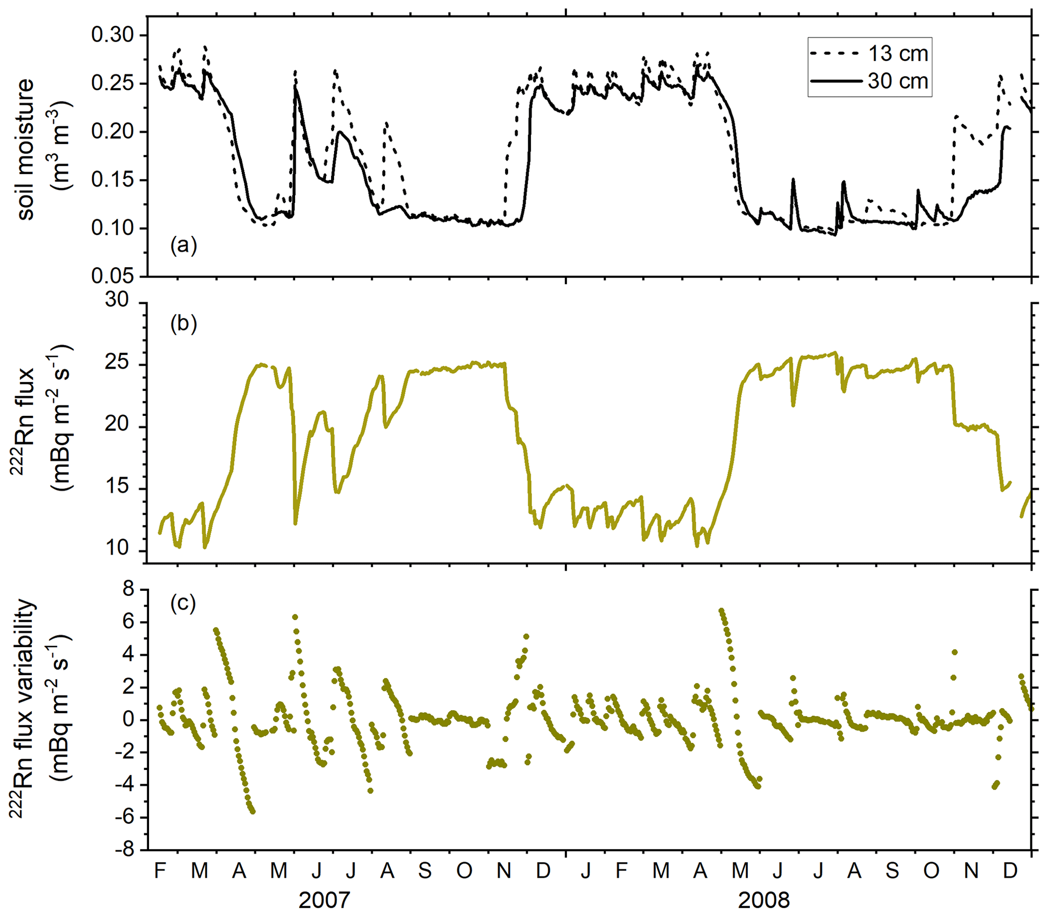
Figure A1 (a) Daily variations of measured soil moisture at the Grenzhof site near Heidelberg at depths of 13 and 30 cm. The hypothetical ²²²Rn flux estimated from the soil moisture (and temperature) variability is shown in (b), while the day-to-day variability around the corresponding monthly means of the ²²²Rn flux is shown in (c). The average variability corresponds to 10 % around the monthly mean flux.