Eastward-propagating planetary waves in the polar middle atmosphere

According to Modern-Era Retrospective Research Analysis for Research and Applications (MERRA-2) temperature and wind datasets in 2019, this study presents the global variations in the eastward-propagating wavenumber 1 (E1), 2 (E2), 3 (E3) and 4 (E4) planetary waves (PWs) and their diagnostic results in the polar middle atmosphere. We clearly demonstrate the eastward wave modes exist during winter periods with westward background wind in both hemispheres. The maximum wave amplitudes in the Southern Hemisphere (SH) are slightly larger and lie lower than those in the Northern Hemisphere (NH). Moreover, the wave perturbations peak at lower latitudes with smaller amplitudes as the wavenumber increases. The period of the E1 mode varies between 3–5 d in both hemispheres, while the period of the E2 mode is slightly longer in the NH (∼ 48 h) than in the SH (∼ 40 h). The periods of the E3 are ∼ 30 h in both the SH and the NH, and the period of E4 is ∼ 24 h. Despite the shortening of wave periods with the increase in wavenumber, their mean phase speeds are relatively stable, ∼ 53, ∼ 58, ∼ 55 and ∼ 52 m/s at 70^∘ latitudes for E1, E2, E3 and E4, respectively. The eastward PWs occur earlier with increasing zonal wavenumber, which agrees well with the seasonal variations in the critical layers generated by the background wind. Our diagnostic analysis also indicates that the mean flow instability in the upper stratosphere and upper mesosphere might contribute to the amplification of the eastward PWs.

1 Introduction

The dominance of large-amplitude planetary waves in the stratosphere, mesosphere and lower-thermosphere regions and their interactions with zonal mean winds are the primary driving forces of atmospheric dynamics. In addition, sudden stratospheric warmings (SSWs) and quasi-biennial oscillation (QBO) events can dynamically couple the entire atmosphere from the lower atmosphere to the ionosphere (Li et al., 2020; Yamazaki et al., 2020; Yadav et al., 2019; Matthias and Ern, 2018; Stray et al., 2015). Westward-propagating planetary waves are one of the prominent features during austral and boreal summer. Westward quasi-2 d waves (Q2DWs) are the most obvious representative waves and one of the most investigated phenomena using planetary wave observations. Most previous studies have focused on the westward-propagating Q2DWs, i.e., zonal wavenumbers of 2 (W2), 3 (W3) and 4 (W4) modes (Lainer et al., 2018; Gu et al., 2018b; Wang et al., 2017; Pancheva et al., 2016; Gu et al., 2016a, b; Lilienthal and Jacobi, 2015; Gu et al., 2013; Limpasuvan and Wu, 2009; Salby, 1981). However, limited studies have been conducted to understand the seasonal variations in the occurrence date, peak amplitude and wave period for the eastward Q2DWs (Gu et al., 2017; Lu et al., 2013; Alexander and Shepherd, 2010; Sandford et al., 2008; Palo et al., 2007; Merzlyakov and Pancheva, 2007; Manney and Randel, 1993; Venne and Stanford, 1979).

Typically, Q2DWs are maximal after the summer solstice in the middle latitudes. The largest wave amplitudes generally appear near the mesopause in January–February in the Southern Hemisphere (SH) and in July–August the Northern Hemisphere (NH) (Tunbridge et al., 2011). W3 and W4 Q2DWs reach amplitudes during austral and boreal summer in the mesosphere and lower thermosphere, respectively. The seasonal variation in westward Q2DW activity is obvious (Liu et al., 2019; Gu et al., 2018b; Rao et al., 2017). By observing the long-term Q2DWs in the NH and SH, Tunbridge et al. (2011) reported that W3 is generally stronger than the other two modes in the SH, reaching an amplitude of ∼ 12 K, while W4 is stronger than W3 in the NH, reaching ∼ 4 K. Moreover, W4 generally lives longer than W3, and W4 can still be observed after the ending of W3. A previous study has demonstrated that the wave source, instability, critical layer and mean zonal wind are the primary reasons for the seasonal variation in Q2DWs (Liu et al., 2004). By studying the long-term satellite datasets in the SH, Gu et al. (2019) have suggested that the strongest events of W2, W3 and W4 could be delayed by increasing the zonal wavenumber, and these events would be indistinguishable during SSWs. The wave periods of W4, W3 and W2 vary at around ∼ 41–56, ∼ 45–52 and ∼ 45–48 h, respectively. Furthermore, W2 can be observed using global satellite datasets, but it has an amplitude that is weaker than W3 and W4 in the NH and SH (Meek et al., 1996). The propagation and amplification of Q2DWs are primarily modulated by the instability, refractive index and critical layer, while the variation in background wind may cause different zonal wavenumber events (Gu et al., 2016a, b). By analyzing the variation in Q2DW activity during SSWs, Xiong et al. (2018) noticed that W1 (westward-propagating wave with wavenumber 1) is generated by the nonlinear interaction between SPW2 (stationary planetary wave with wave number 2) and W3. During SSWs, the coupling between the NH and SH can enhance the summer easterly and promote the nonlinear interaction between W3 and SPW1 (stationary planetary wave with wave number 1) (Gu et al., 2018b).

Some recent studies have discovered significant eastward planetary waves in the polar stratosphere and mesosphere regions, with periods of nearly 2 and 4 d (Gu et al., 2017; Sandford et al., 2008; Merzlyakov and Pancheva, 2007; Coy et al., 2003; Manney and Randel, 1993). Planetary waves with zonal wavenumbers −1 (E1) and −2 (E2) correspond to 4 and 2 d waves, respectively. Furthermore, planetary waves of 1.2 d with wavenumber −3 (E3) and 0.8 d with wavenumber −4 (E4) have been reported to contain the same phase speeds as E1 and E2 (Manney and Randel, 1993). This series of eastward planetary wave can significantly affect the thermal and dynamic structure of the polar stratosphere, resulting in profound changes in its wind and temperature (Coy et al., 2003; Venne and Stanford, 1979). Beyond the knowledge about nonlinear interactions between migrating tides and Q2DWs (Palo et al., 1999), further investigation has confirmed that E2 Q2DW could be generated by the nonlinear interaction between planetary wave and tides in the mesosphere and lower thermosphere (MLT) (Palo et al., 2007). We should note that the E2 Q2DW generated in the MLT region is different from that in the polar stratosphere and is discussed in this paper.

By studying and analyzing satellite datasets, Merzlyakov and Pancheva (2007) indicated that the wave periods of E1 and E2 events range between 1.5–5 d. They reported that Eliassen–Palm (EP) flux travels from the upper to the lower atmosphere, meaning that the upper atmosphere has a dynamic influence on the lower atmosphere. Sandford et al. (2008) reported on significant fluctuations in E2 Q2DWs in the polar mesosphere. They indicated the influence of changes in mean zonal winds during a major SSW on the propagation of polar E2. In addition, they proposed the significance of E2 fluctuation in the mesosphere driven by the instabilities in the polar night jet. For E2, the amplitude of temperature, zonal wind and meridional wind during the austral winter can reach ∼ 10 K, ∼ 20 m/s and ∼ 30 m/s, respectively, while those during the boreal winter can drop by almost two-thirds. Lu et al. (2013) found that eastward planetary wave propagation is limited to the winter high latitudes probably because the negative refractive indices equatorward of ∼ 45^∘ S result in evanescent wave characteristics. That study suggested that the instability region at ∼ 50–60^∘ S might be induced by the stratospheric polar night jet and/or the “double-jet” structure.

In this study, we use the second Modern-Era Retrospective Research Analysis for Research and Applications (MERRA-2) datasets to investigate the eastward-propagating wave characteristics of the stratosphere and mesosphere in polar regions in 2019, including E1, E2, E3 and E4. Specifically, we investigate the variation in the occurrence date, peak amplitude and wave period of eastward waves, as well as the role of instability, background wind structure and the critical layer in the propagation and amplification of eastward waves. The remaining parts of this paper are organized as follows. Section 2 describes the data and methods used in this study. Section 3 analyzes the global latitude–temporal variation structure of eastward waves during winter in 2019. The amplification and propagation features of the eastward planetary waves in the NH and SH with different wavenumber events are examined in Sect. 3.1 and 3.2, respectively. Section 3.3 compares and analyzes the eastward waves in the NH and SH. All research results are summarized in Sect. 4.

2 Data and analysis

To extract the E1, E2, E3 and E4 wave, we apply the least-squares method to each time window (i.e., 10, 6, 4 and 4 d), and then use the time window to determine the amplitude (Gu et al., 2013). This method has been shown to successfully identify planetary waves from satellite measurements (Gu et al., 2019, 2018a, b, c, 2013).

$$\begin{array}{}\text{(1)}& y=A\cos \left[\mathrm{2}\mathit{\pi }\right(\mathit{\sigma }\cdot t+s\cdot \mathit{\lambda }\left)\right]+B\sin \left[\mathrm{2}\mathit{\pi }\right(\mathit{\sigma }\cdot t+s\cdot \mathit{\lambda }\left)\right]+C\end{array}$$

The least-squares method is used to fit the a set of parameters (A, B and C), where σ, t, s and λ are the frequency, UT time, zonal wavenumber and longitudes. The amplitude of wave R can be expressed as $R=\sqrt{A^{\mathrm{2}}+B^{\mathrm{2}}}$.

MERRA-2 covers the long-term atmospheric reanalysis datasets initiated by NASA in 1980. It has been upgraded recently using the Goddard Earth Observing System model, Version 5 (GEOS-5) data assimilation system. Briefly, MERRA-2 includes some updates to the model (Molod et al., 2015, 2012) and the global statistical interpolation (GSI) analysis scheme of Wu et al. (2002). The MERRA-2 data consist of various meteorological variables, e.g., net radiation, temperature, relative humidity and wind speed. The spatial coverage of MERRA-2 data is the globe (spatial resolution, 0.5^∘ × 0.625^∘; temporal resolution, 1 h). These meteorological data are widely used to detect the middle atmosphere such as the planetary wave in the polar atmosphere, global thermal tides, climate variability and aerosol (Ukhov et al., 2020; Sun et al., 2020; Bali et al., 2019; Lu et al., 2013). Many recent studies have indicated the feasibility of using MERRA-2 data for the kind of research in the present study. Therefore, we apply the MERRA-2 datasets to obtain the variation in the background wind, instability, refractive index and critical layer; and we explore the patterns of eastward planetary wave propagation and amplification through diagnostic analysis.

The critical layer will absorb or reflect planetary waves from the lower atmosphere during upward propagation. Planetary waves that gain sufficient energy in the unstable region will be amplified during reflection. In a sense, the critical layer plays an important role in regulating the amplification and propagation of planetary waves (Gu et al., 2016a, b; Liu et al., 2004).

$$\begin{array}{}\text{(2)}& \stackrel{\mathrm{‾}}{q_{\mathit{\phi }}}=\mathrm{2}\mathrm{\Omega }\cos \mathit{\phi }-{\left({\displaystyle \frac{{\left(\stackrel{\mathrm{‾}}{u}\cos \mathit{\phi }\right)}_{\mathit{\phi }}}{a\cos \mathit{\phi }}}\right)}_{\mathit{\phi }}-{\displaystyle \frac{a}{\mathit{\rho }}}{\left({\displaystyle \frac{f^{\mathrm{2}}}{N^{\mathrm{2}}}}\mathit{\rho }\stackrel{\mathrm{‾}}{u_z}\right)}_z\end{array}$$

The baroclinic and/or barotropic instability in the atmospheric space structure is caused by the simultaneous equalization of the negative latitude gradient and the quasi-geostrophic potential vorticity ($\stackrel{\mathrm{‾}}{q_{\mathit{\phi }}})$. In Eq. (2), Ω is the angular speed of the Earth's rotation, φ is the latitude, $\stackrel{\mathrm{‾}}{u}$ is the zonal mean zonal wind, a is the Earth's radius, ρ is the air density, f is the Coriolis parameter, N is the buoyancy frequency, and subscripts z and φ are the vertical and latitudinal gradients.

According to Andrews et al. (1987), the properties of planetary wave propagation can be calculated using the EP flux vectors (F); i.e.,

$$\begin{array}{}\text{(3)}& F=\mathit{\rho }a\cos \mathit{\phi }\left[\begin{array}{l}\frac{\stackrel{\mathrm{‾}}{u_z}\stackrel{\mathrm{‾}}{v^{\prime }{\mathit{\theta }}^{\prime }}}{\stackrel{\mathrm{‾}}{{\mathit{\theta }}_z}}-\stackrel{\mathrm{‾}}{v^{\prime }{u}^{\prime }}\\ \left[f-\frac{{\left(\stackrel{\mathrm{‾}}{u}\cos \mathit{\phi }\right)}_{\mathit{\phi }}}{a\cos \mathit{\phi }}\right]\frac{\stackrel{\mathrm{‾}}{v^{\prime }{\mathit{\theta }}^{\prime }}}{\stackrel{\mathrm{‾}}{{\mathit{\theta }}_z}}-\stackrel{\mathrm{‾}}{w^{\prime }{u}^{\prime }}\end{array}\right],\end{array}$$

where u^′ and v^′ are the planetary wave perturbations in the zonal and meridional wind, respectively, and θ^′ and w^′ are the potential temperature and vertical wind, respectively. The planetary wave propagation is only favorable where the square of the refractive index m² is positive:

$$\begin{array}{}\text{(4)}& m^{\mathrm{2}}={\displaystyle \frac{\stackrel{\mathrm{‾}}{q_{\mathit{\phi }}}}{a\left(\stackrel{\mathrm{‾}}{u}-c\right)}}-{\displaystyle \frac{s^{\mathrm{2}}}{{\left(a\cos \mathit{\phi }\right)}^{\mathrm{2}}}}-{\displaystyle \frac{f^{\mathrm{2}}}{\mathrm{4}{N}^{\mathrm{2}}{H}^{\mathrm{2}}}},\end{array}$$

where s is the zonal wavenumber, c is the phase speed and H is the scale height. The square of the refractive index is taken as the waveguide of planetary waves; i.e.,

$$\begin{array}{}\text{(5)}& c=-{\mathit{\upsilon }}_{\mathrm{0}}\cos \left({\displaystyle \frac{\mathit{\phi }\mathit{\pi }}{\mathrm{180}}}\right)/sT,\end{array}$$

where υ₀ is the equatorial linear velocity, s is the zonal wavenumber and T is the wave period.

3 Results and discussion

We considered the entire period of 2013–2020 and found that the temporal variations in the eastward planetary waves during 2019 are representative of all years in this range. We thus will only present the results for the year 2019. Figure 1 shows the global temporal–latitude variation structures of E1, E2, E3 and E4 extracted from the 2019 MERRA-2 temperature datasets using time windows of 10, 6, 4 and 4 d, respectively. The mean temperature amplitude of E1, E2, E3 and E4 at ∼ 55.4 km during the periods 3–5, 1.5–2.5, 1–1.5 and 0.9–1.1 d are displayed in Fig. 1a, b, c and d, respectively. Eastward waves are characterized by obvious seasonal variations in the SH and NH. In addition, E1, E2 (E3) and E4 reach their maximum amplitude at 50–80^∘ (S and N). In the SH, the strongest E1 and E2 events occur on days 209–218 and 167–172, while E3 and E4 events occur on days 151–154 and 139–142. This means that their occurrence date of maximum amplitude moves earlier with increasing zonal wavenumber. In addition, the maximum amplitude of E1, E2, E3 and E4 are ∼ 6.0, ∼ 4.2, ∼ 3.6 and ∼ 2.4 K, respectively, indicating that their peak amplitudes drop with rising zonal wavenumber. In the NH, the strongest E1, E2, E3 and E4 events occur on days 41–50, 69–74, 35–38 and 63–66, respectively; the corresponding peak amplitudes are ∼ 5.5, ∼ 3.8, ∼ 2.8 and ∼ 1.2 K, respectively. While the results demonstrate the decline in the peak amplitude with increasing zonal wavenumber in the NH, the occurrence date is irregular. Moreover, E4 is relatively weak in the NH and difficult to find, so W4 is insignificant in the NH. Figure 2 presents the changes in zonal mean zonal wind at 70^∘ S and 70^∘ N in 2019. It can be seen that the background wind on days 90–240 (70^∘ S) is dominated by westward wind and reaches ∼ 80 m/s at ∼ 50 km on day 210; it is dominated by eastward wind in late and early 2019 and reaches approximately −40 m/s at ∼ 60 km. Meanwhile, the background wind is primarily westerly in late and early 2019 (70^∘ N) and reaches ∼ 90 m/s at ∼ 60 km on day 50, while on days 120–240, the background wind is primarily easterly wind, and the amplitude reaches −40 m/s on day 200. Compared with Fig. 1, the results show that the eastward wave modes exist during winter periods with westward background wind in both hemispheres.

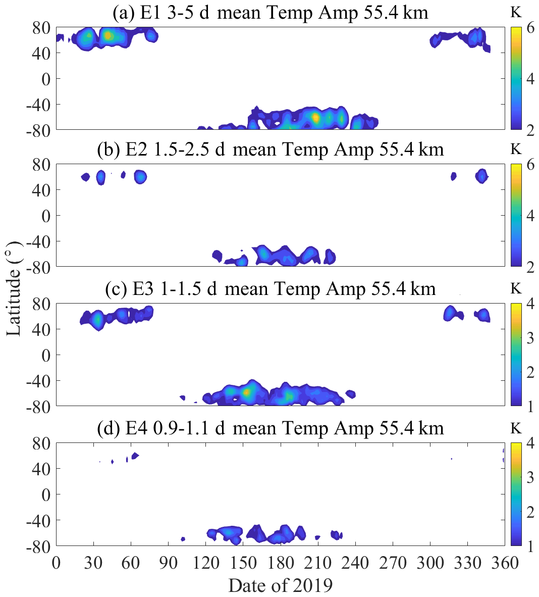
Figure 1 The global latitude–temporal variation structures of the (a) E1, (b) E2, (c) E3 and (d) E4 planetary waves during 2019. White areas represent small-amplitude data (corresponds to the right color bar). The date indicates the day of the year.

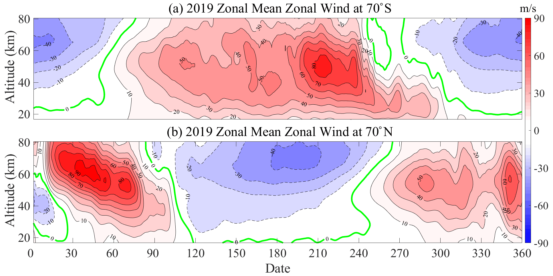
Figure 2 The zonal mean zonal wind variations of (a) 70^∘ S and (b) 70^∘ N during 2019. The dashed lines represent eastward wind; the solid black lines represent westward wind; and the solid green line is 0 m/s. The date indicates the day of the year.

3.1 In the Southern Hemisphere

Figure 3 shows that the observed maximum temperature amplitude is at ∼ 48.2 km and ∼ 70–80^∘ S for E1, ∼ 48.2 km and ∼ 60–70^∘ S for E2 and E3, and ∼ 48.2 km and ∼ 50–60^∘ S for E4. For E1, the observed maximum perturbation occurs on days 211–220 (with an amplitude of ∼ 8.5 K), and the remaining fluctuations occur on days 161–170, 187–196 and 231–240. For E2, the observed maximum perturbation happens at days 219–224 (with an amplitude of ∼ 7.8 K), and three peaks appear on days 139–144, 173–178 and 187–192. Regarding E3, the strongest perturbation occurs on days 151–154 (with an amplitude of ∼ 5.2 K) and the other events are distributed on days 141–144, 201–204 and 209–202. E4 perturbations are distributed on days 127–130, 145–148, 161–164 and 213–216, with a weak amplitude of ∼ 3 K. Since earlier studies mentioned that the wave period of the eastward wave can vary, we also investigate the periodic variabilities in E1, E2, E3 and E4. The results show that the period corresponding to the maximum perturbation of E1 falls between ∼ 106 (days 187–196) and ∼ 69 h (days 211–220), and their wave periods vary significantly. Nonetheless, the wave period of E2 gradually changes from ∼ 42 (days 139–144) to ∼ 38 h (days 219–224), and its stability is stronger than that of E1. The wave periods of E3 and E4 are about ∼ 39 and ∼ 24 h, respectively. These results reflect that the E2, E3 and E4 wave periods are more stable compared to E1.

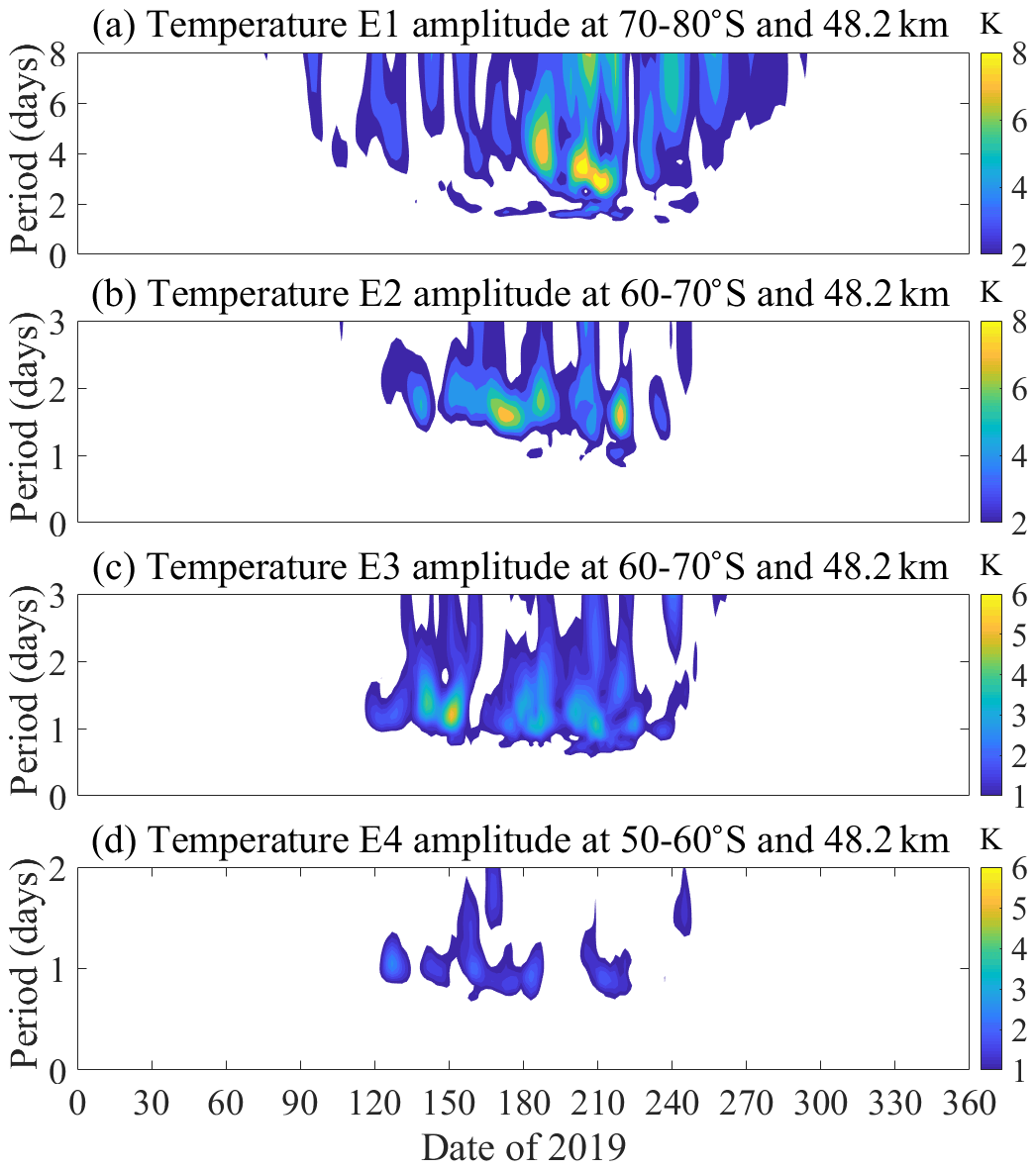
Figure 3 The temporal variations in (a) E1, (b) E2, (c) E3 and (d) E4 during the 2019 austral winter period. The date indicates the day of the year.

The spectra, spatial (vertical and latitudinal) structures of temperature, zonal and meridional wind, and diagnostic analysis of E1 are extracted from the two corresponding events (refer to Fig. 4). Figure 4a and b show the least-squares fitting spectra for MERRA-2 temperature on days 187–196 and 211–220 at ∼ 48.2 km and ∼ 70–80^∘ S, when and where the E1 is maximal. An eastward wavenumber −1 signal with the periods of ∼ 106 and ∼ 69 h clearly dominates the whole spectrum. The temperature spatial structures corresponding to these E1 periods (i.e., ∼ 106 and ∼ 69 h) are displayed in Fig. 4c and d. The temperature spatial structure of E1 exhibits obvious amplitude bimodal structure at ∼ 70–80^∘ S and ∼ 50 km and ∼ 70–80^∘ S and ∼ 60 km, with the maximum at ∼ 70–80^∘ S and ∼ 50 km. The strongest temperature amplitude of E1 occurs at ∼ 50 km and ∼ 70–80^∘ S with an amplitude of ∼ 10 K on days 211–220, and the other peak is ∼ 9 K (∼ 70–80^∘ S and ∼ 60 km). The temperature amplitude of ∼ 9 K occurs at ∼ 50 km and ∼ 70–80^∘ S during days 187–196, and the other events have a temperature amplitude of ∼ 7 K (∼ 70–80^∘ S and ∼ 60 km). The corresponding spatial structures of zonal wind and meridional wind of these E1 events are shown in Fig. 4e–h. The maximum zonal wind amplitude of E1 occurs at ∼ 60–70^∘ S and ∼ 60 km with an amplitude of ∼ 14 m/s on days 187–196 and ∼ 20 m/s at ∼ 50–60^∘ S and ∼ 60 km on days 211–220. The amplitude of E1 meridional wind hits ∼ 10 m/s at ∼ 70–80^∘ S and ∼ 55 km (days 187–196) and ∼ 17 m/s at ∼ 70–80^∘ S and ∼ 60 km (days 211–220).

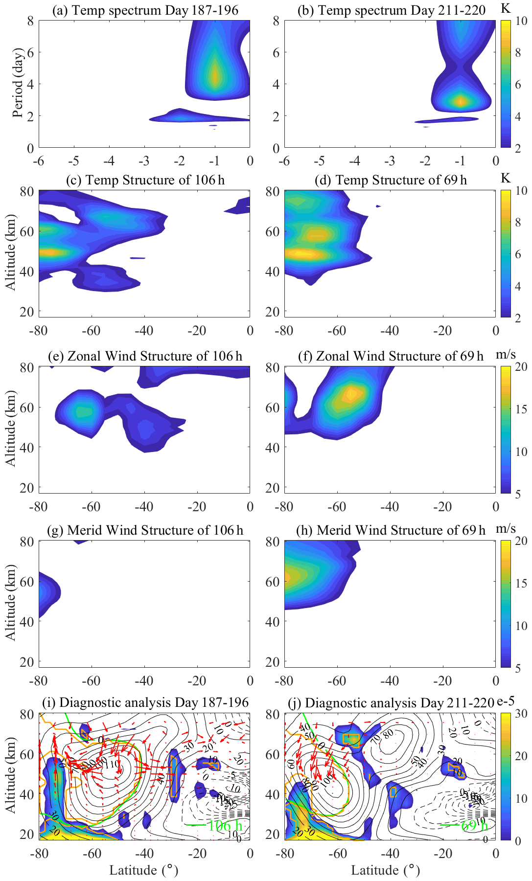
Figure 4 The (a, b) spectra, (c, d) temperature spatial structures, (e, f) zonal wind spatial structures, (g, h) meridional wind spatial structures and (i, j) diagnostic analysis of the E1 typical events during the 2019 austral winter period. The MERRA-2 temperature data observations at 48.2 km and 70–80^∘ S during days 187–196 (Fig. 4a), 211–220 (Fig. 4d) are utilized. In the diagnostic analysis of E1 events, the blue-shaded regions are instability, the red arrows are EP flux, and the green line is the critical layer. The green line represents critical layers of E1 with the natural period. Regions enclosed by solid orange lines are characterized by the positive refractive index for E1.

Figure 4i and j show the diagnostic analysis results for the E1 events during days 187–196 and 211–220, respectively. Apparently, the EP flux vectors are more favorable to propagation in the SH winter and are dramatically amplified by the mean flow instabilities and appropriate background winds in the polar region and between ∼ 40 and ∼ 80 km, with EP flux propagating into the upper atmosphere (Fig. 4i). Meanwhile, there is an EP flux at the mid-latitudes and ∼ 60–80 km, which propagates into the lower atmosphere. The wave–mean flow interaction near its critical layer (106 h) of the green curve amplifies E1, and the positive-refractive-index region surrounded by the yellow curve also enhances E1 propagation. In addition, the strong instability and weak background wind at ∼ 70–80^∘ S and ∼ 40–60 km provide sufficient energy for the upward EP flux to propagate and amplify. Nevertheless, the downward-propagating EP flux is amplified by weak instability and strong background wind at ∼ 50–60^∘ S and ∼ 60–70 km. Besides, both upward and downward EP fluxes eventually propagate toward the Equator at ∼ 50 km. Figure 4j shows that EP flux on days 211–220 propagates downward and amplifies after the interaction of the critical layer (∼ 69 h). The positive-refractive-index region, strong instability and weak background wind at ∼ 50–60^∘ S and ∼ 60–70 km provide sufficient energy for E1 amplification and propagation and ultimately point toward the Equator at ∼ 50 km. The results show that the weak background wind and strong instability in the polar region can promote the upward propagation and amplification of EP flux. Meanwhile, the appropriate background wind and instability in the mid-latitudes are also conducive to the downward propagation and amplification of EP flux. In other words, instability and appropriate background wind dominate the propagation and amplification of E1.

For E2, the spectra are observed at ∼ 48.2 km and ∼ 60–70^∘ S on days 173–178 and 219–224 when the eastward wavenumber −2 becomes the primary wave mode with the wave periods ∼ 38 and ∼ 39 h, respectively (as shown in Fig. 5a, b). The temperature spatial structures corresponding to these E2 periods (∼ 38 and ∼ 39 h) are presented in Fig. 5c and d. The temperature spatial structure of E2 shows an obvious amplitude bimodal structure at ∼ 60–70^∘ S and ∼ 50 km and ∼ 60–70^∘ S and ∼ 60 km, with the maximum at ∼ 60–70^∘ S and ∼ 50 km. The maximum temperature amplitude of E1 occurs at ∼ 50 km and ∼ 60–70^∘ S with an amplitude of ∼ 7.5 K on days 173–178, and the other peak is ∼ 6 K (∼ 70^∘ S and ∼ 60 km). The temperature amplitude of ∼ 10 K happens at ∼ 50 km and ∼ 60–70^∘ S during days 219–224, and the other events have a temperature amplitude of ∼ 6 K (∼ 70^∘ S and ∼ 60 km). The corresponding spatial structures of zonal wind and meridional wind of these E2 events are illustrated in Fig. 5e–h. The zonal wind spatial structure of E2 shows an obvious amplitude bimodal structure at ∼ 50–60^∘ S and ∼ 60 km and ∼ 70–80^∘ S and ∼ 60 km, with the maximum at ∼ 50–60^∘ S and ∼ 60 km. The maximum zonal wind amplitude of E2 appears at ∼ 50–60^∘ S and ∼ 60 km with an amplitude of ∼ 10 m/s on days 173–178, and the other peak is ∼ 9 m/s (∼ 70–80^∘ S and ∼ 60 km). The zonal wind amplitude of ∼ 20 m/s occurs at ∼ 50–60^∘ S and ∼ 60 km on days 219–224, and the other events have a zonal wind amplitude of ∼ 15 m/s (∼ 70–80^∘ S and ∼ 60 km). The amplitude of E2 meridional wind reaches ∼ 13 m/s at ∼ 70–80^∘ S and ∼ 60 km (days 173–178) and ∼ 27 m/s at ∼ 70–80^∘ S and ∼ 60 km (days 219–224).

Figure 5 Same as Fig. 4 but for E2 during the 2019 austral winter period.

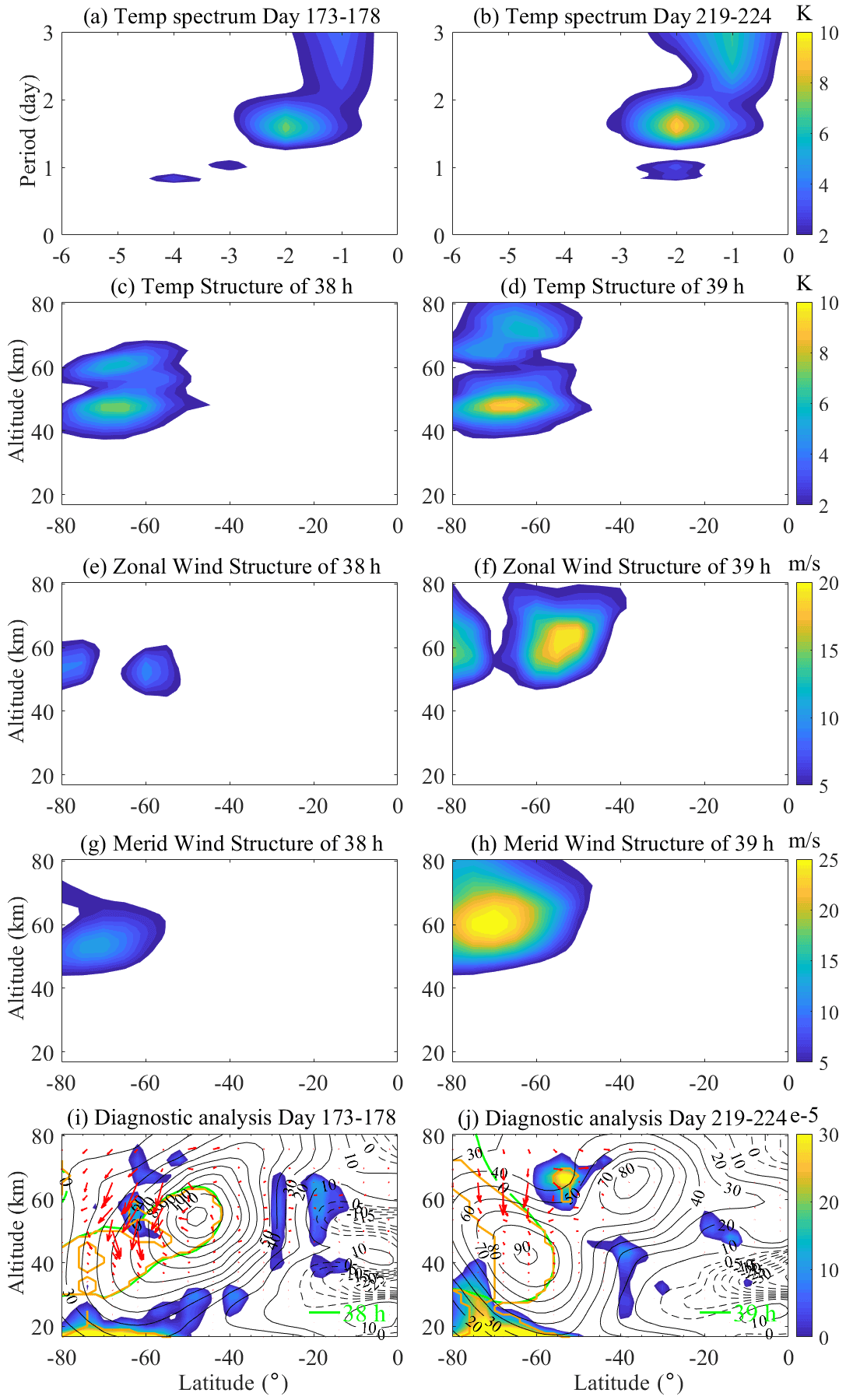
Figure 5i and j illustrate the diagnostic analysis during days 173–178 and 219–224, respectively, for E2. Obviously, E2 is more likely to propagate in the SH winter and is dramatically amplified by the mean flow instabilities at the middle–high latitudes between ∼ 40 and ∼ 80 km. With EP flux propagating into the lower atmosphere, it eventually propagates toward the Equator at ∼ 50 km. Besides, E2 is amplified and propagated by the wave–mean flow interactions near its critical layer (∼ 38 h) of the green curve and the promoting effect of the positive-refractive-index region surrounded by the yellow curve. Meanwhile, the weak instability and strong background wind at ∼ 50–60^∘ S and ∼ 50–70 km provide the energy for the propagation and amplification of EP flux into the lower atmosphere during days 173–178 (Fig. 5i). According to the diagnostic analysis of days 219–224, E2 obtains sufficient energy from strong instability and strong background wind at ∼ 50–60^∘ S and ∼ 60–70 km. It is amplified and propagated into the lower atmosphere through the critical layer and positive-refractive-index action (as shown in Fig. 5j). The results show that the background wind at ∼ 50–60^∘ S and ∼ 50–70 km is weaker on days 173–178 than on days 219–224; and the instability at ∼ 50–60^∘ S and ∼ 60–70 km is stronger on days 219–224 than on days 173–178. Our results show that E2 has absorbed sufficient energy to be amplified under the background conditions during days 219–224 (Fig. 5a, b).

Figure 6a and b show the observed spectra of E3 at ∼ 48.2 km and ∼ 60–70^∘ S on days 151–154 and 201–204, and the wave periods of locked wavenumber −3 are ∼ 29 and ∼ 29 h, respectively. The corresponding temperature spatial structures of these E3 periods (i.e., ∼ 29 and ∼ 29 h) are displayed in Fig. 6c and d. The temperature spatial structure of E3 shows an obvious amplitude bimodal structure at ∼ 60–70^∘ S and ∼ 50 km, and ∼ 60–70^∘ S and ∼ 60 km, with the maximum at ∼ 60–70^∘ S and ∼ 50 km. Besides, E3 also has a weak peak at ∼ 60–70^∘ S and ∼ 70 km. The strongest temperature amplitude of E3 occurs at ∼ 50 km and ∼ 60–70^∘ S with an amplitude of ∼ 6 K on days 151–154, and the other peak is ∼ 5 K (∼ 60–70^∘ S and ∼ 60 km). The temperature amplitude of ∼ 5 K happens at ∼ 50 km (∼ 60 km) and ∼ 60–70^∘ S during days 201–204. The corresponding spatial structures of zonal wind and meridional wind of these E3 events are shown in Fig. 6e–h. The zonal wind spatial structure of E3 shows an obvious amplitude bimodal structure at ∼ 70–80^∘ S and ∼ 60 km and ∼ 50–60^∘ S and ∼ 60 km. The zonal wind amplitudes of E3 occur at ∼ 70–80^∘ S and ∼ 60 km (∼ 50–60^∘ S and ∼ 60 km) with an amplitude of ∼ 9 m/s on days 151–154 and ∼ 9 m/s at ∼ 70–80^∘ S and ∼ 60 km (∼ 50–60^∘ S and ∼ 60 km) on days 201–204. The amplitude of E3 meridional wind hits ∼ 13 m/s at ∼ 60–70^∘ S and ∼ 55 km (days 151–154) and ∼ 16 m/s at ∼ 60–70^∘ S and ∼ 55 km (days 201–204).

Figure 6 Same as Fig. 4 but for E3 during the 2019 austral winter period.

The EP flux of E3 is similar to that of E2. The instability and appropriate background wind at the middle–high latitudes between ∼ 50 km and ∼ 70 km dramatically amplify the propagation of E3, which is enhanced by the interaction near the critical layer (∼ 29 h) and the positive-refractive-index region (Fig. 6i and j). Notably, the strong instability and weak background wind at ∼ 50–60^∘ S and ∼ 60–70 km on days 151–154 provide sufficient energy for the propagation and amplification of EP flux into the lower atmosphere and ultimately point toward the Equator at 50 km. During days 201–204, the EP flux propagates into the lower atmosphere and is amplified by interaction at the critical layer (∼ 29 h). Besides, weak instability and weak background wind at ∼ 50–60^∘ S and ∼ 60–70 km provide the energy to amplify the E3 propagation. Figure 6c and d indicate that the stronger the instability at ∼ 50–60^∘ S and ∼ 60–70 km, the stronger the temperature amplitude of E3. We believe that the background wind and instability at ∼ 50–60^∘ S and ∼ 60–70 km are the main reasons for the propagation and amplification of EP flux into the lower atmosphere.

For E4, the spectra appear at ∼ 48.2 km and ∼ 50–60^∘ S on days 127–130 and 213–216 when the eastward wavenumber −4 signal has a wave period of ∼ 25 and ∼ 21 h (see Fig. 7a, b). The corresponding temperature spatial structures of these E4 periods (i.e., ∼ 25 and ∼ 21 h) are shown in Fig. 7c and d. The temperature spatial structure of E4 shows an obvious amplitude bimodal structure at ∼ 50–60^∘ S and ∼ 50 km and ∼ 50–60^∘ S and ∼ 60 km, with the maximum at ∼ 50–60^∘ S and ∼ 50 km. The maximum temperature amplitude of E4 occurs at ∼ 50 km and ∼ 50–60^∘ S with an amplitude of ∼ 4 K on days 127–130, and the other peak is ∼ 3 K (∼ 60–70^∘ S and ∼ 60 km). The temperature amplitude of ∼ 3 K occurs at ∼ 50 km (∼ 60 km) during days 213–216. The corresponding spatial structures of zonal wind and meridional wind of these E4 events are presented in Fig. 7e–h. The zonal wind spatial structure of E4 shows an obvious amplitude bimodal structure at ∼ 50–60^∘ S and ∼ 55 km and ∼ 60–70^∘ S and ∼ 55 km, with the maximum at ∼ 50–60^∘ S and ∼ 55 km. The maximum zonal wind amplitude of E4 happens at ∼ 50–60^∘ S and ∼ 55 km with an amplitude of ∼ 9 m/s on days 127–130, and the other peak is ∼ 5 K (∼ 60–70^∘ S and ∼ 55 km). The zonal wind amplitude of ∼ 5 m/s occurs at ∼ 50–60^∘ S (∼ 60–70^∘ S) and ∼ 55 km on days 213–216. The amplitude of E4 meridional wind reaches ∼ 8 m/s at ∼ 60–70^∘ S and ∼ 55 km (days 127–130) and ∼ 10 m/s at ∼ 60–70^∘ S and ∼ 55 km (days 213–216).

Figure 7 Same as Fig. 4 but for E4 during the 2019 austral winter period.

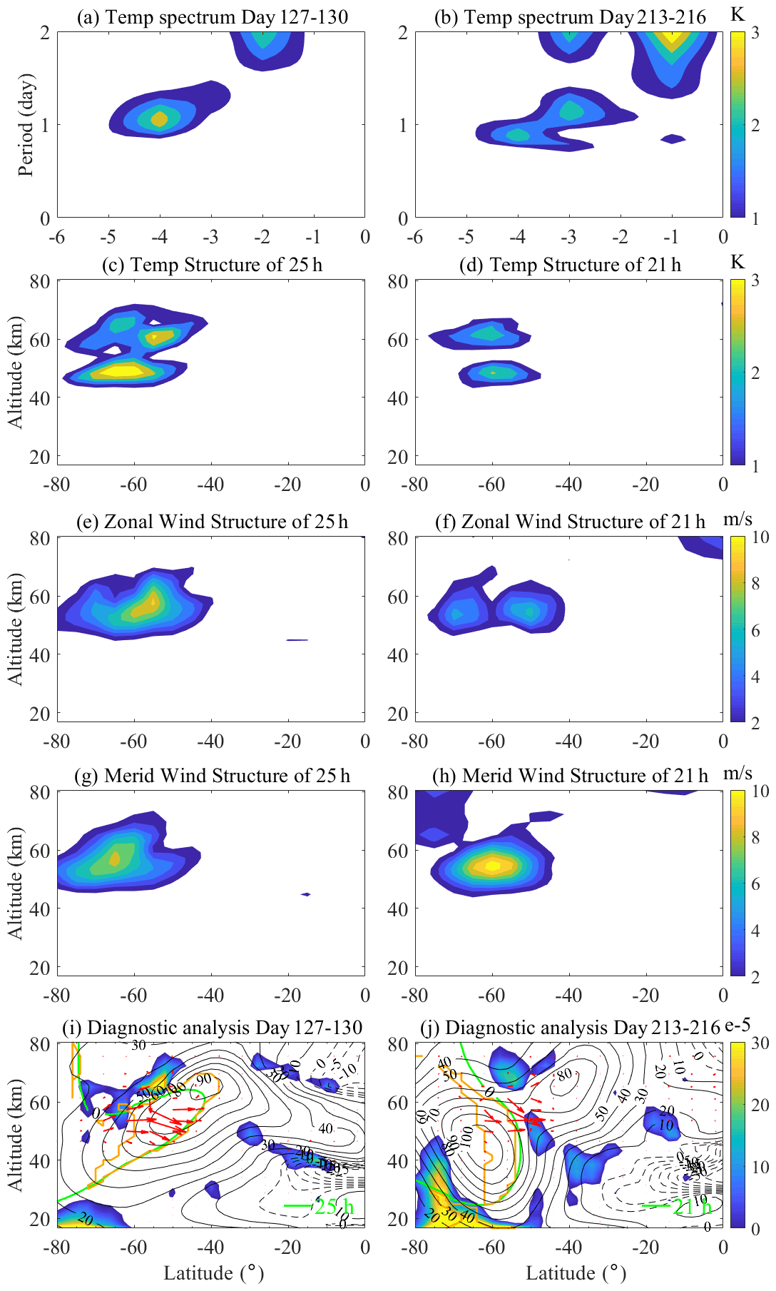
Diagnostic analysis for E4 on days 127–130 and 213–216 is shown in Fig. 7i and j, respectively. The results demonstrate that E4 is dramatically amplified by the mean flow instabilities at the middle–high latitudes between ∼ 50 and ∼ 70 km. With EP flux propagating into the lower atmosphere, it finally propagates toward the Equator at ∼ 50 km. E4 is amplified and propagated by the wave–mean flow interaction near the critical layer (∼ 25 and ∼ 21 h), and the positive-refractive-index region generates the promoting effect. The strong instability and weak background wind at ∼ 50–60^∘ S and ∼ 60–70 km provide sufficient energy for the propagation and amplification of EP flux into the lower atmosphere during days 127–130. Besides, E4 obtains energy from weak instability and weak background wind at ∼ 50–60^∘ S and ∼ 60–70 km on days 213–216, and it is amplified and propagated into the lower atmosphere. The background wind at ∼ 50–60^∘ S and ∼ 60–70 km on days 127–130 is similar to on days 213–216, and the instability at ∼ 50–60^∘ S and ∼ 60–70 km is stronger on days 127–130 than on days 213–216. According to Fig. 7a and b, E4 absorbs sufficient energy to be amplified under the background conditions on days 127–130, and the temperature amplitude on days 127–130 is stronger.

3.2 In the Northern Hemisphere

Figure 8 shows that the observed maximum temperature amplitude appears at ∼ 59.2 km and ∼ 70–80^∘ N for E1, and E2 and E3 peak at ∼ 59.2 km and ∼ 60–70^∘ N. The maximum perturbation of E1 occurs on days 41–50 (with an amplitude of ∼ 8 K), while the remaining fluctuations occur on days 25–34 and 339–348. Besides, the strongest E2 event occurs on days 69–74 (with an amplitude of ∼ 7 K), and the other events are distributed on days 25–30, 317–322 and 341–346. By contrast, E3 is maximal on days 35–38 (with an amplitude of ∼ 3 K) and also shows a peak on days 53–56. Based on the study of the wave period in the SH for eastward waves, the periodic variabilities in E1, E2 and E3 in the NH are also examined. The wave period of E1 decreases from a maximum of ∼ 118 h (days 25–34) to ∼ 80 h (days 41–50), indicating the instability of the wave period of E1 in the NH. The E2 events occur on days 25–30, 69–74, 317–322 and 341–346, of which the corresponding wave periods are ∼ 36, ∼ 53, ∼ 52 and ∼ 48 h, which are stronger and more stable than E1. Besides, the wave period of E3 is relatively stable at ∼ 29 and ∼ 27 h. Thus, the E2 and E3 wave periods are more stable than that of E1.

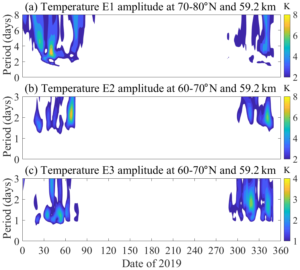
Figure 8 The temporal variations in (a) E1, (b) E2 and (c) E3 QTDWs during the 2019 boreal winter period. The date indicates the day of the year.

The spectra, spatial (vertical and latitudinal) structures of temperature, zonal and meridional wind, and diagnostic analysis of E1 are extracted from the corresponding representative events (as shown in Fig. 9). Figure 9a and b show the observed spectra of E1 at ∼ 59.2 km and ∼ 70–80^∘ N on days 25–34 and 41–50, and the wave periods of locked wavenumber −1 are ∼ 118 and ∼ 80 h, respectively. The corresponding temperature spatial structures of these E1 periods (∼ 118 and ∼ 80 h) are shown in Fig. 9c and d. The temperature spatial structure of E1 shows an obvious amplitude bimodal structure during days 25–34 at ∼ 60–70^∘ N and ∼ 60 km and ∼ 40–50^∘ N and ∼ 70 km, with the maximum at ∼ 60–70^∘ N and ∼ 60 km. On top of that, E1 also has bimodal structure on days 41–50 at ∼ 60–70^∘ N and ∼ 60 km and ∼ 60–70^∘ N and ∼ 70 km. The strongest temperature amplitude of E1 occurs at ∼ 60–70^∘ N and ∼ 60 km with an amplitude of ∼ 7 K on days 25–34, and the other peak is ∼ 4 K (∼ 40–50^∘ N and ∼ 70 km). The temperature amplitude of ∼ 10 K occurs at ∼ 60 km and ∼ 60–70^∘ N during days 41–50, and the other events have a temperature amplitude of ∼ 8 K (∼ 60–70^∘ N and ∼ 70 km). The corresponding spatial structures of zonal wind and meridional wind of these E1 events are illustrated in Fig. 9e–h. The zonal wind spatial structure of E1 presents an obvious amplitude bimodal structure at ∼ 70–80^∘ N and ∼ 70 km and ∼ 50–60^∘ N and ∼ 70 km. The zonal wind amplitude of ∼ 13 m/s occurs at ∼ 70–80^∘ N and ∼ 70 km on days 25–34, and the other events have a zonal wind amplitude of ∼ 10 m/s (∼ 50–60^∘ N and ∼ 70 km). In addition, there is a weak peak of 9 K during days 25–34 (∼ 30–40^∘ N and ∼ 70 km). The maximum zonal wind amplitude of E1 occurs at ∼ 70–80^∘ N and ∼ 70 km with an amplitude of ∼ 19 m/s on days 41–50, and the other peak is ∼ 13 K (∼ 50–60^∘ N and ∼ 70 km). The amplitude of E1 meridional wind hits ∼ 14 m/s at ∼ 70–80^∘ N and ∼ 70 km (days 25–34) and ∼ 22 m/s at ∼ 70–80^∘ N and ∼ 70 km (days 41–50).

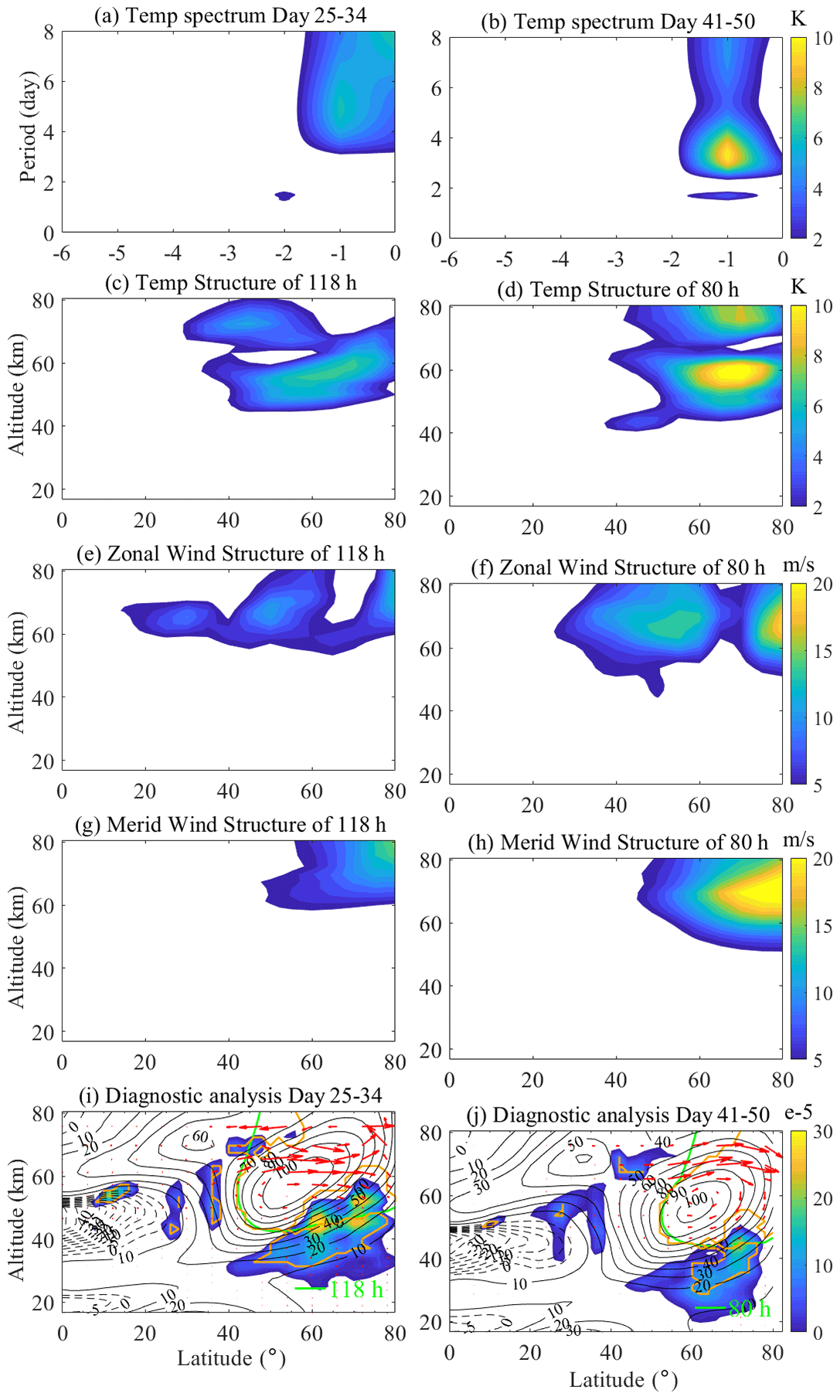
Figure 9 The (a, b) spectra, (c, d) temperature spatial structures, (e, f) zonal wind spatial structures, (g, h) meridional wind spatial structures and (i, j) diagnostic analysis of the E1 typical events during the 2019 boreal winter period. The E1 events at 48.2 km and 70–80^∘ N were obtained from the MERRA-2 reanalysis.

The diagnostic analysis results for E1 (in Fig. 9i and j) suggest the dramatic amplification of E1 by the mean flow instabilities at the middle–high latitudes between ∼ 50 km and ∼ 70 km. With the propagation of EP flux into the polar lower atmosphere, it eventually propagates toward the Equator at ∼ 50 km. The wave–mean flow interaction near the critical layers (∼ 118 and ∼ 80 h) amplifies and propagates E1, and the promoting effect of the positive-refractive-index region amplifies E1. Furthermore, the weak instability and strong background wind at ∼ 40–50^∘ N and ∼ 60–70 km generate the energy for the propagation and amplification of EP flux into the polar lower atmosphere during days 25–34. E1 obtains sufficient energy from weak instability and suitable background wind on days 41–50 at ∼ 40–50^∘ N and ∼ 60–70 km and is amplified and propagated into the polar lower atmosphere through the critical layer and positive-refractive-index action. The background wind at ∼ 40–50^∘ N and ∼ 60–70 km is stronger on days 25–34 than on days 41–50, but its instability is similar, indicating that stronger background winds might weaken E1 propagation and amplification at the middle–northern latitudes. Our results show that E1 absorbs adequate energy to be amplified under the background conditions during days 41–50, reflecting a stronger temperature amplitude (see Fig. 9a, b).

For E2, the spectra are at ∼ 59.2 km and ∼ 60–70^∘ N on days 25–30 and 69–74 when the eastward wavenumber −2 signal has the periods ∼ 36 and ∼ 53 h (as shown in Fig. 10a, b). The corresponding temperature spatial structures of these E2 periods (i.e., ∼ 36 and ∼ 53 h) are presented in Fig. 10c and d. The temperature spatial structure of E2 demonstrates an obvious amplitude bimodal structure at ∼ 60–70^∘ N and ∼ 60 km, and ∼ 60–70^∘ N and ∼ 70 km, with the maximum at ∼ 60–70^∘ N and ∼ 60 km. The maximum temperature amplitude of E2 occurs at ∼ 60–70^∘ N and ∼ 60 km with an amplitude of ∼ 5 K on days 25–30, and the other peak is ∼ 4 K (∼ 60–70^∘ N and ∼ 70 km). The temperature amplitude of ∼ 9 K occurs on days 69–74 at ∼ 60^∘ S and ∼ 60 km, and the other peaks are ∼ 7 K (∼ 60–70^∘ N and ∼ 70 km) and ∼ 5 K (∼ 60–70^∘ N and ∼ 50 km). The corresponding spatial structures of zonal wind and meridional wind of these E2 events are shown in Fig. 10e–h. The zonal wind spatial structure of E2 shows an obvious amplitude bimodal structure at ∼ 60–70^∘ N and ∼ 60 km and ∼ 40–50^∘ N and ∼ 60 km, with the maximum at ∼ 40–50^∘ N and ∼ 60 km. The maximum zonal wind amplitude of E2 appears at ∼ 60–70^∘ N and ∼ 60 km (∼ 40–50^∘ N and ∼ 60 km) with an amplitude of ∼ 6 m/s on days 25–30. Zonal wind amplitude occurs at ∼ 40–50^∘ N and ∼ 60 km with an amplitude of ∼ 18 m/s on days 41–50, and the other peak is ∼ 16 K (∼ 60–70^∘ N and ∼ 60 km). The amplitude of E2 meridional wind reaches ∼ 7 m/s at ∼ 60–70^∘ N and ∼ 70 km (days 25–30) and ∼ 18 m/s at ∼ 60–70^∘ N and ∼ 60 km (days 41–50).

Figure 10 Same as Fig. 9 but for E2 during the 2019 boreal winter period.

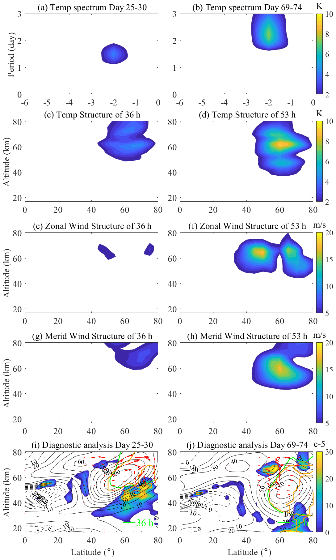
The diagnostic analysis of E2 on days 25–30 and 69–74 is shown in Fig. 10i and j, respectively. Apparently, E2 is significantly amplified by the mean flow instabilities at the middle–high latitudes between ∼ 40 and ∼ 70 km, with EP flux propagating into the polar lower atmosphere, and EP flux eventually propagates toward the Equator at ∼ 50 km. E2 is amplified and propagated by the wave–mean flow interaction near the critical layers (∼ 36 and ∼ 53 h), and the positive-refractive-index region provides the promoting effect. The weak instability and strong background wind at ∼ 50–60^∘ N and ∼ 60–70 km provide the energy for the propagation and amplification of EP flux into the polar lower atmosphere during days 25–30. Moreover, E2 obtains sufficient energy from strong instability and suitable background wind at ∼ 50–60^∘ N and ∼ 60–70 km on days 69–74, and it is amplified and propagated into the polar lower atmosphere. The background wind at ∼ 50–60^∘ N and ∼ 60–70 km on days 127–130 is similar to on days 213–216, and the instability at ∼ 50–60^∘ S and ∼ 60–70 km is stronger on days 127–30 than on days 213–216. Although the background wind at ∼ 50–60^∘ N and ∼ 60–70 km is stronger on days 25–30 than on days 69–74, the instability at ∼ 50–60^∘ N and ∼ 60–70 km is stronger on days 69–74 than on days 25–30. The temperature amplitude results indicate that E2 absorbs sufficient energy to be amplified under the background conditions on days 69–74, with a stronger temperature amplitude on days 69–74 (Fig. 10a, b).

Figure 11a and b show the observed spectra of E3 at ∼ 59.2 km and ∼ 60–70^∘ N on days 35–38 and 53–56, and the wave periods of locked wavenumber −3 are ∼ 29 and ∼ 27 h, respectively. The corresponding temperature spatial structures of these E3 periods (i.e., ∼ 29 and ∼ 27 h) are shown in Fig. 11c and d. The temperature spatial structure of E3 shows an obvious amplitude bimodal structure at ∼ 50–60^∘ N and ∼ 60 km and ∼ 50–60^∘ N and ∼ 70 km, with the maximum at ∼ 50–60^∘ N and ∼ 60 km. The strongest temperature amplitude of E3 occurs at ∼ 60 km and ∼ 50–60^∘ N with an amplitude of ∼ 6 K on days 35–38, and the other peak is ∼ 5 K (∼ 50–60^∘ N and ∼ 70 km). The temperature amplitude of ∼ 4 K occurs at ∼ 60 km (∼ 70 km) and ∼ 50–60^∘ N during days 53–56. The corresponding spatial structures of zonal wind and meridional wind of these E3 events are illustrated in Fig. 6e–h. The zonal wind spatial structure of E3 shows an obvious amplitude bimodal structure at ∼ 40–50^∘ N and ∼ 70 km and ∼ 60–70^∘ N and ∼ 70 km. The zonal wind amplitudes of E3 occur at ∼ 40–50^∘ N and ∼ 70 km with an amplitude of ∼ 15 m/s on days 35–38 and ∼ 12 m/s at ∼ 60–70^∘ N and ∼ 70 km. The maximum zonal wind amplitude of E3 appears at ∼ 40–50^∘ N and ∼ 70 km (∼ 60–70^∘ N and ∼ 70 km) with an amplitude of ∼ 7 m/s (∼ 6 m/s) on days 53–56. The amplitude of E3 meridional wind reaches ∼ 22 m/s at ∼ 50–60^∘ N and ∼ 70 km (days 35–38) and ∼ 12 m/s at ∼ 60–70^∘ N and ∼ 70 km (days 53–56).

Figure 11 Same as Fig. 9 but for E3 during the 2019 boreal winter period.

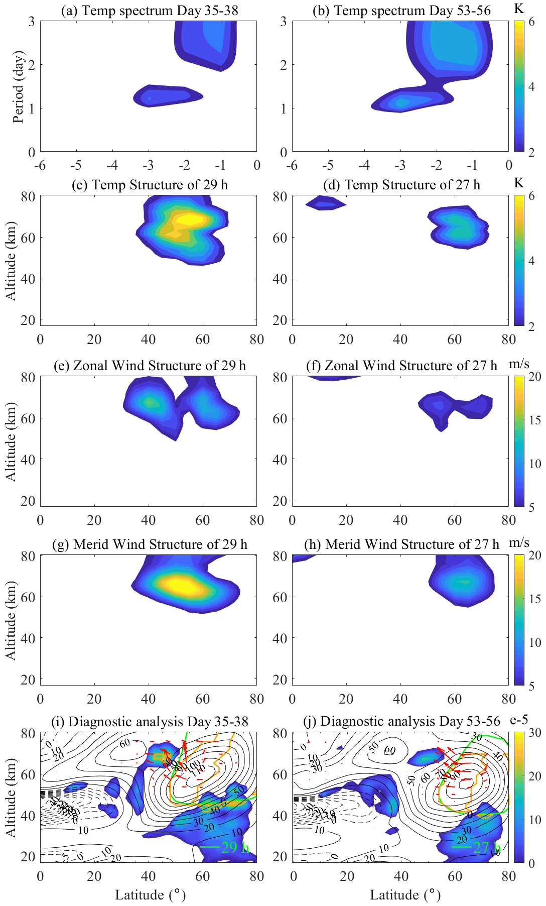
Obviously, the instability and appropriate background wind at the mid-latitudes between ∼ 50 and ∼ 70 km and the interaction near the critical layers (∼ 29 and ∼ 27 h) dramatically amplify the propagation of E3 (see Fig. 11i and j). The background wind is similar on days 35–38 and 53–56, and the former period is relatively unstable. This finding indicates that E3 in propagation is more likely to gather sufficient energy to be amplified on days 35–38. The instability and appropriate background wind at the middle–high latitudes between ∼ 50 and ∼ 70 km drastically amplify the propagation of E3, which is enhanced by the interaction near the critical layers (∼ 29 and ∼ 27 h) and the positive-refractive-index region (Fig. 11i, j). In particular, the strong instability and weak background wind at ∼ 50–60^∘ N and ∼ 60–70 km on days 35–38 generate sufficient energy for the propagation and amplification of EP flux into the lower atmosphere and ultimately point toward the Equator at 50 km. The EP flux propagates to the lower atmosphere during days 35–38, and it is amplified by interactions at the critical layer (∼ 29 h). In addition, weak instability and weak background winds on days 53–56 at ∼ 50–60^∘ N and ∼ 60–70 km provide the energy to amplify E3 propagation. Combined with Fig. 11c and d, the stronger the instability at ∼ 50–60^∘ N and ∼ 60–70 km, the stronger the temperature amplitude of E3. The results show that the instability on days 35–38 at ∼ 50–60^∘ N and ∼ 60–70 km is the primary reason for the propagation and amplification of EP flux into the lower atmosphere.

3.3 Comparison between SH and NH

The observed latitude and maximum temperature amplitude for eastward planetary waves (i.e., E1, E2, E3, E4) decrease and weaken with increasing zonal wavenumber in the SH, reaching ∼ 70–80, ∼ 60–70, ∼ 60–70 and ∼ 50–60^∘ S and ∼ 10, ∼ 9, ∼ 6 and ∼ 3 K, respectively. In addition, the occurrence date moves earlier with increasing zonal wavenumber. The temperature spatial structure demonstrates a bimodal-peak structure (∼ 50 and ∼ 60 km), mainly located at ∼ 50 km. The maximum zonal wind amplitudes of E1 and E2 and of E3 and E4 are almost the same, ∼ 20 and ∼ 10 m/s, respectively. The maximum meridional wind amplitudes of E1, E2, E3 and E4 are ∼ 17, ∼ 27, ∼ 16 and ∼ 11 m/s, respectively. The wave period of E1 tends to become shorter from 5 to 3 d, while E2 and E3 are close to ∼ 40 and ∼ 30 h and E4 remains at ∼ 24 h. E1, E2, E3 and E4 are more favorable to propagation in the SH winter and are abruptly amplified by the mean flow instabilities at the middle latitudes between ∼ 40 and ∼ 70 km. With the propagation of EP flux into the lower atmosphere, it finally propagates toward the Equator at ∼ 50 km. In addition, the propagation of EP flux for E1 to the upper atmosphere might be influenced by the instability and background wind at the Antarctic at ∼ 50 km.

The observed latitudes of E1 and E2 (E3) decrease with increasing wavenumber in the NH, at ∼ 70–80 and ∼ 60–70^∘ N (∼ 60–70^∘ N). With a bimodal-peak structure located at ∼ 70 km, the temperature spatial structures of E1, E2 and E3 reach ∼ 10, ∼ 9 and ∼ 6 K, respectively. The maximum zonal wind amplitudes for E1, E2 and E3 occur at ∼ 50–80^∘ N and ∼ 70 km, and their amplitudes are almost equal to ∼ 18 m/s. The maximum meridional winds of E1, E2 and E3 occur at ∼ 50–80^∘ N and ∼ 70 km with amplitudes of ∼ 22 m/s, ∼ 18 m/s and ∼ 22 m/s, respectively. The wave period of E1 tends to be shorter at 5–3 d, and E2 and E3 are close to ∼ 48 and ∼ 30 h. In addition, E1, E2 and E3 are more favorable to propagation in the NH winter and are dramatically amplified by the mean flow instabilities at the middle latitudes between ∼ 40 and ∼ 70 km, with the propagation of EP flux into the lower atmosphere and then toward the Equator at ∼ 50 km.

4 Summary and conclusions

Based on the MERRA-2 temperature and wind observations in 2019, we present for the first time an extensive study of the global variation in eastward planetary wave activity, including E1, E2, E3 and E4 in the stratosphere and mesosphere. We presented the analysis results only for the year 2019 due to the representative of the wave activities for the entire range of 2013–2020. The temperature and wind amplitude and wave periods of each event were determined using 2-D least-squares fitting. Our study covered the spatial and temporal patterns of the eastward planetary waves in both hemispheres with a comprehensive diagnostic analysis on their propagation and amplification. The key findings of this study are summarized below.

The latitudes for the maximum (temperature, zonal and meridional wind) amplitudes of E1, E2, E3 and E4 decrease with increasing wavenumber in the SH and NH. The E1, E2, E3 and E4 events occur earlier with increasing zonal wavenumber in the SH. In addition, eastward wave modes exist during summer periods with westward background wind in both hemispheres.

The temperature spatial structures of E1, E2, E3 and E4 present a double-peak structure, which is located at ∼ 50 and ∼ 60 km in the SH and ∼ 60 and ∼ 70 km in the NH. Furthermore, the lower peak is usually larger than the higher one.

The maximum (temperature, zonal and meridional wind) amplitudes of E1, E2 and E3 decline with rising zonal wavenumber in the SH and NH. The maximum temperature amplitudes in the SH are slightly larger and lie lower than those in the NH. In addition, the meridional wind amplitudes are slightly larger than those of the zonal wind in the SH and NH.

The wave period of the E1 mode ranges between 3–5 d in both hemispheres, while the period of the E2 mode is slightly longer in the NH (∼ 48 h) than in the SH (∼ 40 h). The periods of E3 in both SH and NH are ∼ 30 h, while the period of E4 is ∼ 24 h.

The eastward planetary wave is more favorable to propagation in the winter hemisphere and is drastically amplified by the mean flow instabilities and appropriate background winds in the polar region and the middle latitudes between ∼ 40 and ∼ 80 km. Furthermore, the amplification of planetary waves through wave–mean flow interaction occurs easily close to their critical layer. In addition, the direction of EP flux ultimately points toward the Equator.

The strong instability and appropriate background wind in the lower layer of the Antarctic region might generate adequate energy to promote E1 propagation and amplification to the upper atmosphere.

Overall, this study demonstrated how the background zonal wind in the polar middle atmosphere affects the dynamics of eastward planetary waves in the polar middle atmosphere.