Model emulation to understand the joint effects of ice-nucleating particles and secondary ice production on deep convective anvil cirrus

Ice crystal formation in the mixed-phase region of deep convective clouds can affect the properties of climatically important convectively generated anvil clouds. Small ice crystals in the mixed-phase cloud region can be formed by heterogeneous ice nucleation by ice-nucleating particles (INPs) and secondary ice production (SIP) by, for example, the Hallett–Mossop process. We quantify the effects of INP number concentration, the temperature dependence of the INP number concentration at mixed-phase temperatures, and the Hallett–Mossop splinter production efficiency on the anvil of an idealised deep convective cloud using a Latin hypercube sampling method, which allows optimal coverage of a multidimensional parameter space, and statistical emulation, which allows us to identify interdependencies between the three uncertain inputs.

Our results show that anvil ice crystal number concentration (ICNC) is determined predominately by INP number concentration, with the temperature dependence of ice-nucleating aerosol activity having a secondary role. Conversely, anvil ice crystal size is determined predominately by the temperature dependence of ice-nucleating aerosol activity, with INP number concentration having a secondary role. This is because in our simulations ICNC is predominately controlled by the number concentration of cloud droplets reaching the homogeneous freezing level which is in turn determined by INP number concentrations at low temperatures. Ice crystal size, however, is more strongly affected by the amount of liquid available for riming and the time available for deposition growth which is determined by INP number concentrations at higher temperatures. This work indicates that the amount of ice particle production by the Hallett–Mossop process is determined jointly by the prescribed Hallett–Mossop splinter production efficiency and the temperature dependence of ice-nucleating aerosol activity. In particular, our sampling of the joint parameter space shows that high rates of SIP do not occur unless the INP parameterisation slope (the temperature dependence of the number concentration of particles which nucleate ice) is shallow, regardless of the prescribed Hallett–Mossop splinter production efficiency. A shallow INP parameterisation slope and consequently high ice particle production by the Hallett–Mossop process in our simulations leads to a sharp transition to a cloud with extensive glaciation at warm temperatures, higher cloud updraughts, enhanced vertical mass flux, and condensate divergence at the outflow level, all of which leads to a larger convectively generated anvil comprised of larger ice crystals. This work highlights the importance of quantifying the full spectrum of INP number concentrations across all mixed-phase altitudes and the ways in which INP and SIP interact to control anvil properties.

1 Introduction

Deep convective clouds are an important component of the global hydrological cycle and radiative budget (e.g. Lohmann et al., 2016; Massie et al., 2002). The anvil cirrus cloud they produce can persist in the atmosphere for several hours to a few days and therefore impact outgoing radiation long after the deep convection has decayed (Luo and Rossow, 2004). However, accurately representing the spatial and temporal complexity of large convective systems and therefore convectively generated cirrus presents extensive challenges for atmospheric modelling (Prein et al., 2015).

Deep convective cloud systems extend vertically from the boundary layer to the tropopause and can have a horizontal radius of over 1000 km. They are dynamic and powerful systems with updraught speeds of up to 50 m s⁻¹ (Frank, 1977; Musil et al., 1986; Xu et al., 2001). In addition, a multitude of different thermodynamic and microphysical conditions can exist within the same system. There is also a scarcity of measurements of these climatically important clouds, particularly profile measurements within the convective core (Fan et al., 2016), and thus a scarcity of data with which to validate representations of deep convective clouds in models. The myriad of competing microphysical processes operating within deep convective clouds, along with the difficulty in validating model simulations against observations, cause the simulation of deep convective clouds to be subject to a large number of parametric and structural uncertainties (Johnson et al., 2015; Wellmann et al., 2018). In particular, mixed-phase microphysics presents a challenge for cloud modelling because it is critical for deep convective cloud properties and poorly understood (Prein et al., 2015).

One of the largest uncertainties in quantifying aerosol–cloud interactions and the resultant climate impacts is the amount of, and balance between, liquid and ice in mixed-phase clouds. In particular, the representation of microphysical processes affecting cloud phase in tropical convection contributes substantial uncertainty to the simulated climate response to global warming in climate models (Medeiros et al., 2008; Stevens and Bony, 2013). The representation of the amount of ice within deep convective clouds is also important for the representation of the amount and intensity of precipitation, the prediction of which is one of the most socially and economically important roles of numerical weather forecasting (Arakawa, 2004; Prein et al., 2015).

Within the mixed-phase region of deep convective clouds, i.e. the region between 0 and ∼ −38 ^∘C where both liquid and ice can coexist, we hypothesise that three factors controlling ice production strongly influence the partitioning of condensate into cloud liquid and ice, which are listed as follows.

• i.

  The limiting number concentration of ice-nucleating particles (INPs: aerosol particles with the ability to initiate the freezing of cloud droplets at mixed-phase temperatures) at the top of the mixed-phase cloud regime (in this work, this is the INP number concentration at −38 ^∘C). In an aerosol population made up entirely of dust particles, all with ice-nucleating potential, the limiting number concentration of INP would equate to the number concentration of dust.

• ii.

  The temperature dependence of the INP number concentration at mixed-phase temperatures (the rate of increase in ambient INP number concentrations as temperature decreases from ∼ 0 to ∼ −38 ^∘C). This determines the concentration of INP at lower mixed-phase altitudes and therefore the altitude of liquid depletion due to heterogeneous freezing in the lower and middle mixed-phase cloud levels (e.g. Hawker et al., 2021; Takeishi and Storelvmo, 2018).

• iii.

  The efficiency of ice production by secondary ice production (SIP) mechanisms, whereby small ice particles are produced from existing frozen hydrometeors (Field et al., 2017), such as ice crystals frozen heterogeneously, or larger snow and graupel particles.

The limiting number concentration of INPs in the atmosphere is extremely variable and depends on several interacting factors. For example, Saharan dust is an efficient INP at temperatures below −15 ^∘C and the largest component by mass of the global aerosol budget (Tang et al., 2016; Textor et al., 2006). The export of this atmospherically important INP, across the Atlantic Ocean, varies hugely depending on factors such as season (Ridley et al., 2012); desert soil moisture (Laurent et al., 2008); local wind speed (Grini et al., 2005; Laurent et al., 2008); and the occurrence and intensity of convection, wet removal, and dry deposition (Bou Karam et al., 2014; Marsham et al., 2011; Provod et al., 2016), both in source (Heinold et al., 2013) and transport regions (Sauter et al., 2019; Twohy and Twohy, 2015). As a result of variations in dust emission and transport, summertime INP number concentrations in the Saharan Air Layer can vary by up to 4 orders of magnitude at −33 ^∘C (Boose et al., 2016). Variations in INP number concentrations can impact cloud properties and cloud radiative forcing (e.g. Shi and Liu, 2019; Solomon et al., 2018). However, the reported effect of changes to INP number concentrations on cloud properties can be non-linear, counterintuitive, or conflicting depending on the environmental conditions, magnitude of the tested perturbation, or study methodology (Deng et al., 2018; Fan et al., 2010a, b; Gibbons et al., 2018; Hawker et al., 2021; van den Heever et al., 2006; Phillips et al., 2005, 2007).

The temperature dependence of INP number concentration depends, amongst other factors, on the aerosol type providing INP in a given scenario. A large number of aerosol types have the ability to act as INPs, including mineral dust (Atkinson et al., 2013; Niemand et al., 2012; Price et al., 2018; Welti et al., 2018), organic material in sea spray (McCluskey et al., 2018; Wilson et al., 2015), bacteria (Šantl-Temkiv et al., 2015), and pollen (Diehl et al., 2002). INPs comprised of marine organics emitted with sea spray tend to have a shallower temperature dependence than INP comprised of mineral dusts. This means marine organic INPs tend to have a higher ice-nucleating ability than mineral dust INPs at warm temperatures but lower ice-nucleating ability at colder temperatures (Atkinson et al., 2013; DeMott et al., 2016; McCluskey et al., 2018; Niemand et al., 2012; Vergara-Temprado et al., 2017; Wilson et al., 2015). In numerical weather and climate models, the temperature dependence of INP number concentration can be described by the slope of the INP parameterisation (i.e. $\mathrm{d}\left({\log }_{\mathrm{10}}{N}_{\text{INP}}\right)/\mathrm{d}T$, as described in Hawker et al., 2021). The INP parameterisation slope depends on aerosol type (DeMott et al., 2010; Harrison et al., 2016, 2019) and any ageing the aerosol has been subjected to (Boose et al., 2016; Brooks et al., 2014) as well as particle properties yet to be fully understood, such as surface morphology (Holden et al., 2019). The INP slope of any one aerosol population (composed of different INP types) is extremely uncertain and difficult to accurately predict without specific measurements. Variation in ice nucleation active site densities (n_s) even of materials of similar mineralogy can span several orders of magnitude at any one temperature (Atkinson et al., 2013; Harrison et al., 2016, 2019). The factors governing active site location and densities are not fully understood but are theorised to be related to features on an INP surface such as surface pits (Holden et al., 2019), hydrophilic sites (Freedman, 2015), or lattice mismatches (Kulkarni et al., 2015). Variations in the temperature dependence of INP number concentration can affect the cloud development and the altitude at which cloud glaciation occurs, as was noted by Takeishi and Storelvmo (2018). This difference in glaciation altitude has been shown to cause differences in hail amount, intensity, and size (Liu et al., 2018); anvil ice crystal number concentration (N_ice) (Takeishi and Storelvmo, 2018); and radiative forcing (Hawker et al., 2021) of convective clouds.

Observational campaigns have long documented the existence of ice crystals at concentrations vastly exceeding the concentration of INP in clouds with relatively warm cloud top temperatures, indicating the presence of SIP mechanisms (e.g. Crawford et al., 2012; Field et al., 2017; Huang et al., 2017; Ladino et al., 2017; Lasher-Trapp et al., 2016). SIP can occur via processes such as rime splintering (i.e. the Hallett–Mossop process), droplet shattering, collision fragmentation, and sublimation fragmentation (Field et al., 2017; Korolev et al., 2020; Korolev and Leisner, 2020). The most well-studied SIP mechanism is the Hallett–Mossop process by which small ice splinters are produced during the riming of liquid drops onto existing frozen hydrometeors (Crawford et al., 2012; Field et al., 2017; Hallett and Mossop, 1974; Ladino et al., 2017; Phillips et al., 2007). However, even the Hallett–Mossop process is relatively poorly defined and its importance disputed. A recent laboratory study failed to observe rime splintering in conditions designed to stimulate the Hallett–Mossop process (Emersic and Connolly, 2017), and some recent literature suggests that previous observations of ice crystal number concentration attributed to the Hallett–Mossop process may have been indicative of other secondary ice formation mechanisms (Korolev et al., 2020). Nevertheless, as it is the only SIP mechanism that is currently represented in most numerical weather prediction (NWP) models, we focus on the uncertainty associated with the Hallett–Mossop process in this study.

In addition to the individual uncertainties in INP number concentration, INP temperature dependence, and SIP rates, these three factors can also interact causing non-linear or counterintuitive changes in cloud properties, further motivating the exploration of their combined effects here. For example, intermediate INP number concentrations and intermediate Hallett–Mossop ice production rates have been found to produce higher cloud ice crystal number concentrations (ICNC) than high INP number concentrations or high SIP rates alone due to non-linear interactions between the two freezing mechanisms whereby very high heterogeneous freezing rates affect the availability and efficiency of secondary ice production, and vice versa (Crawford et al., 2012; Sullivan et al., 2017).

We investigate the individual and interacting effects of the INP number concentration, the temperature dependence of INP number concentration across the full spectrum of mixed-phase temperatures, and the Hallett–Mossop ice production efficiency on the micro- and macro-physical properties of an idealised deep convective cloud by conducting a large ensemble of idealised simulations using Latin hypercube sampling to select the input parameter combinations and using statistical emulation where appropriate to analyse the ensemble output. We quantify the importance of the three uncertain input parameters and their interactions with one another for the anvil properties of the simulated deep convective cloud. Our methodology proves to be a powerful tool for analysing and understanding the behaviour of complex systems (Johnson et al., 2015; Lee et al., 2011; Marshall et al., 2019; Wellmann et al., 2018) because Latin hypercube sampling enables dense sampling over a defined parameter uncertainty space, allowing more extensive coverage of the defined parameter space than a traditional one-at-a-time test, and statistical emulation allows the production of detailed response surfaces of system behaviours across the three dimensions.

This paper is structured as follows: Sect. 2 describes the idealised cloud model and the simulation set-up, as well as the methods used in our analysis. In Sect. 3, we examine the role of the uncertain input parameters in determining the ice crystal number concentration, ice crystal size, and the cloud fraction of the simulated deep convective anvil cirrus. In Sect. 4, we detail the limitations of our study. Section 5 summarises the main findings and implications of this study.

2 Methods

2.1 Model set-up and simulation design

This work utilises the Met Office NERC Cloud Model (MONC), which is a large Eddy simulation (LES) model with interactive cloud microphysics and radiation. While, the underpinning science of MONC is based on the Met Office Large Eddy Model (LEM) (Gray et al., 2001), MONC is a complete redesign of the LEM, which incorporates a pluggable component architecture to improve usability and is designed to be highly scalable (Brown et al., 2015, 2018). Here, MONC is coupled to the Met Office Cloud AeroSol Interacting Microphysics (CASIM) module, which is a multi-moment bulk scheme. MONC–CASIM has been used to investigate aerosol–cloud interactions in nocturnal fog (Poku et al., 2019) and low-level clouds during the West African monsoon season (Dearden et al., 2018). CASIM has also been used with the Met Office Unified Model in regional simulations of coastal mixed-phase convective clouds (Miltenberger et al., 2018a, b), south-east Pacific stratocumulus clouds (Grosvenor et al., 2017), Southern Ocean supercooled shallow cumulus (Vergara-Temprado et al., 2018), mid-latitude cyclones (McCoy et al., 2018), cloud condensation nuclei (CCN)-limited Arctic clouds (Stevens et al., 2018), and tropical convective clouds (Hawker et al., 2021).

The simulations presented use a grid box spacing of 250 m (500 × 500 grid boxes) and 138 vertical levels. The model diagnostics are output every 5 min, and the time step is flexible to maintain model stability with a maximum value of 2 s and a minimum value of 0.01 s. MONC–CASIM is configured to be a two-moment scheme in this work. The number and mass concentrations for cloud droplets, rain droplets, ice crystals (or cloud ice), graupel, and snow are prognostic variables. The prognostic aerosol variables utilised in this work are the soluble accumulation-mode aerosol mass and number concentrations and the coarse mode dust mass and number concentrations. The aerosol can be advected around, but in the simulations presented here we choose to switch off scavenging processes, and the aerosol is therefore not incorporated into the cloud droplets when activated. The model boundary conditions are cyclical, and as such scavenging the aerosol would result in a rapid removal of all aerosol from the simulation.

The CASIM model configuration is very similar to that of Hawker et al. (2021). Cloud droplet nucleation is parameterised according to Abdul-Razzak and Ghan (2000). The soluble accumulation mode aerosol is used for cloud droplet activation, and a simplistic CCN activation parameterisation is included for the insoluble aerosol mode that assumes a 5 % soluble fraction on dust. Condensation is represented using saturation adjustment, meaning that where water saturation is exceeded at the end of a time step, the specific humidity is adjusted to be the equilibrium saturation over water and the grid box temperature and liquid mass is adjusted accordingly. If only frozen hydrometeors are present in a grid box, saturation is treated explicitly. Collision–coalescence, riming of ice crystals producing graupel, and aggregation of ice crystals producing snow are represented. Rain drop freezing is described using the parameterisation of Bigg (1953). Deposition onto ice and snow is treated explicitly allowing ice particles to grow in ice-supersaturated conditions including in the presence of liquid. Heterogeneous freezing (via immersion freezing) is active between −38 and −3 ^∘C in the MONC–CASIM model used in this work and is described in more detailed in Sect. 2.2.1 and 2.2.2. The INP parameterisations resulting from the perturbations described in Sect. 2.2.1 and 2.2.2 inspect the conditions (temperature, cloud droplet number, ICNC) and aerosol concentrations within a grid box and use that information to predict an ice production rate via heterogeneous freezing. The supercooled droplets are depleted by the freezing parameterisation, but scavenging of INPs is not represented. As stated above, inclusion of scavenging was not possible as due to the cyclical boundary conditions of the simulation, scavenging processes would result in the rapid depletion of aerosol from the domain. The consideration of the number of ice crystals already present as well as the number of INP available when calculating the rate of heterogeneous freezing in a grid box acts as a control on the number of heterogeneous ice crystals forming in the absence of scavenging. Homogeneous freezing of cloud droplets is parameterised according to Jeffery and Austin (1997).

Radiative processes are represented by the Suite of Community RAdiative Transfer codes based on Edwards and Slingo (SOCRATES) (Edwards and Slingo, 1996; Manners et al., 2017), which in this study considers all five hydrometeor types for the calculation of cloud radiative properties. Changes in size and number of cloud droplets are considered. The cloud droplet single scattering properties are calculated from the cloud droplet mass and effective radius in each grid box using the equations detailed in Edwards and Slingo (1996). A fixed effective radius of 30 µm for ice crystals is used in the radiation calculations. For the other hydrometeor types (snow, graupel, rain), SOCRATES considers changes in mass but does not explicitly consider changes in number concentration or size (though changes in number and size will affect mass concentrations which are considered). As the use of SOCRATES in MONC including the radiative effects of ice hydrometeors has not been extensively tested, we do not examine the radiative diagnostic outputs or present them in this paper. Large-scale wind shear is prescribed and constant throughout the simulation. The Coriolis force is inactive in the simulations, and large-scale subsidence is determined by the local column theta.

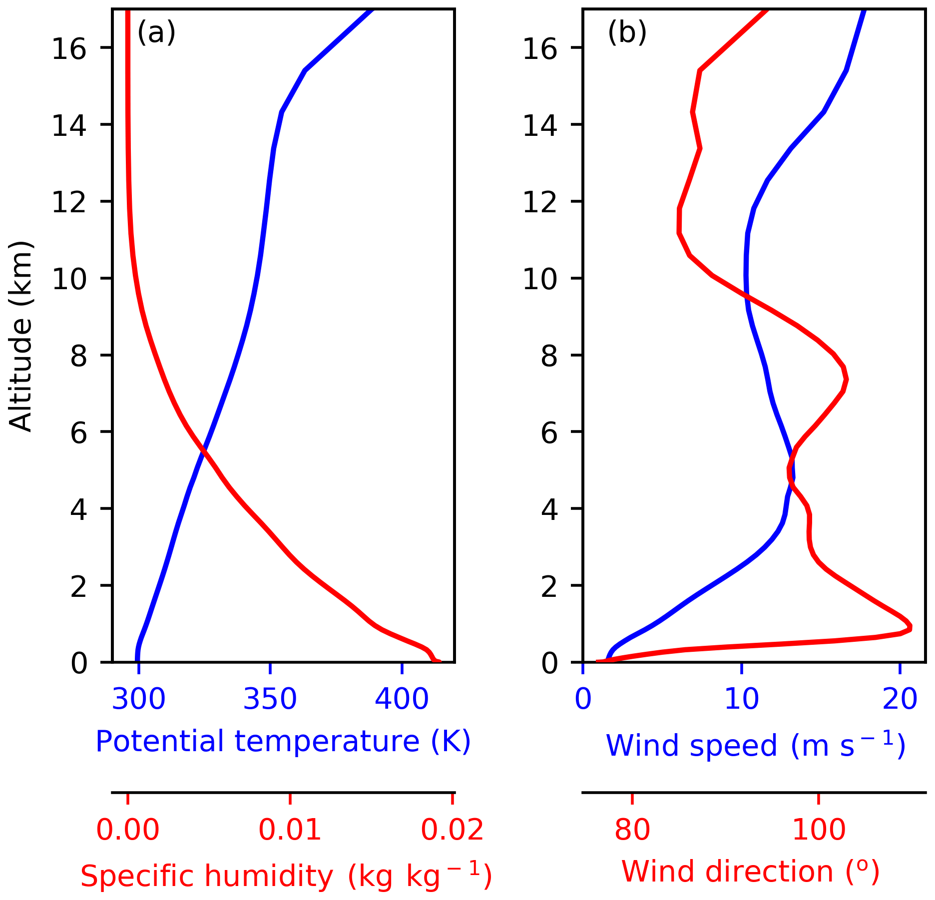
Figure 1 Initial conditions. The potential temperature and specific humidity (a) and wind speed and direction (b) profiles used to initiate the model. The profiles shown were extracted from a Met Office Unified Model simulation of a large deep convective cloud field in the maritime tropical Atlantic (described in Hawker et al., 2021). The profiles were averaged over out-of-cloud areas between 12:00 and 18:00 UTC.

We simulate a single deep convective cloud using the MONC–CASIM model. The cloud formation is initiated using a single warm bubble with a radius of 20 km, a height of 500 m, and a temperature perturbation of 1.5 ^∘C. The model was initiated using mean profiles (wind velocity and direction, potential temperature, specific humidity, and soluble accumulation mode aerosol number and mass concentration) extracted from a Met Office Unified Model simulation of a deep convective cloud field sampled during the “Ice in Clouds Experiment – Dust” flight campaign on the 21 August 2015 (between 12:00 and 15:00 UTC) (Hawker et al., 2021). Details of this simulation including comparisons to observations are available in Hawker et al. (2021). The environmental conditions used to initiate the model are shown in Fig. 1.

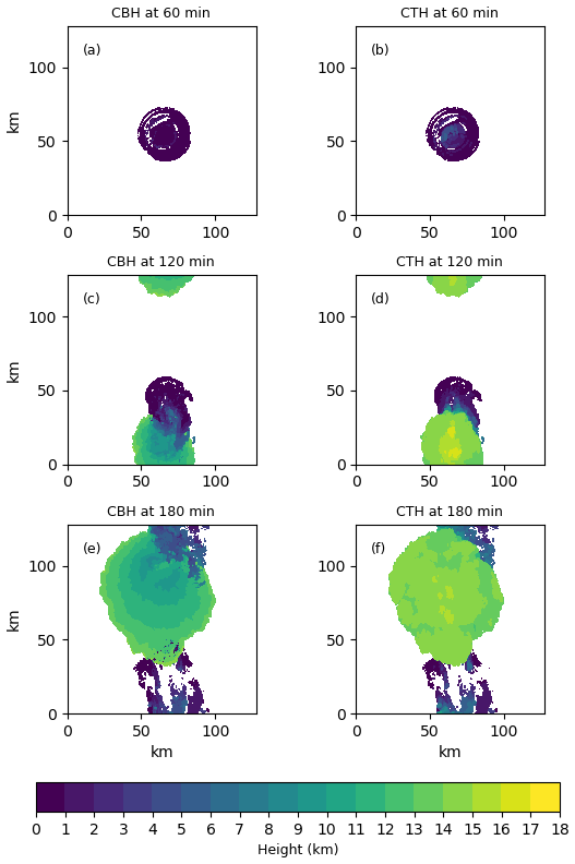
Figure 2 Cloud evolution. The cloud base height (CBH panels, a, c, and e) and cloud top height (CTH panels, b, d, and f) of the simulated convective cloud for the base case simulation.

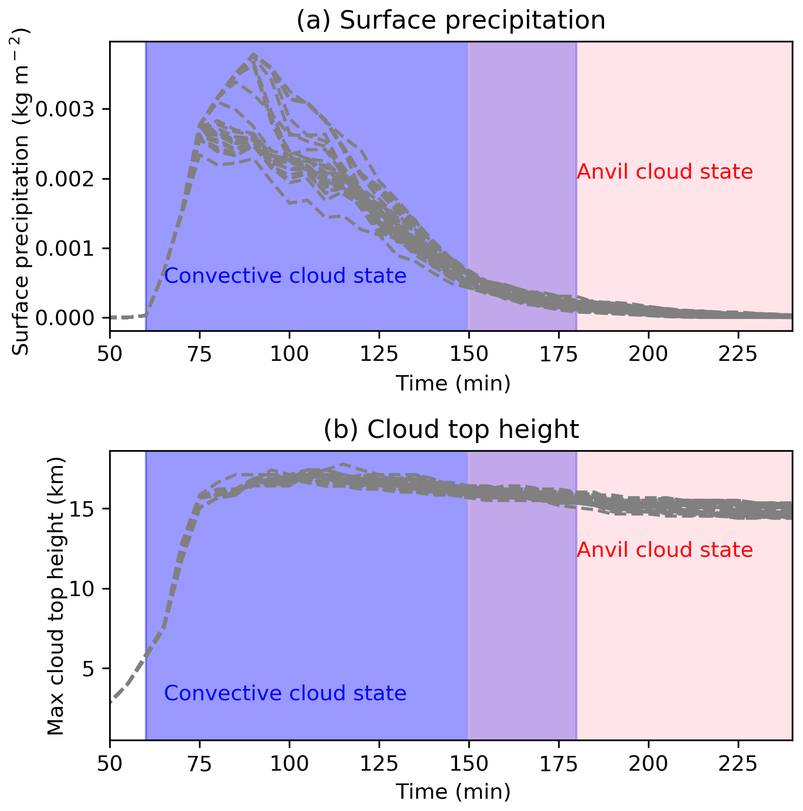
Figure 3 Simulated cloud properties. Evolution of surface precipitation in all cloudy regions (a) and maximum cloud top height (b) over time for all simulations included in analysis. The convective and anvil cloud stages defined for the purposes of analysis are highlighted.

The simulation produces a large convective cloud with an extensive anvil (Fig. 2). Figure 3 shows that the cloud evolution for all simulations is similar with a large increase in surface precipitation (Fig. 3a) from 60 to up to 90 min and a decline that begins between 70 and 90 min. Similarly, the maximum cloud top height for most simulations peaks at around 120 min and afterwards declines slightly, indicating a reduction in convective strength (Fig. 3b). It is important for statistical emulation (Sect. 2.4), where one value for each cloud response is extracted from the model, that the clouds in each simulation undergo similar life cycles. We can see from Fig. 3 that this is the case for the simulated deep convective cloud.

Table 1 Target output variables. List of target output variables discussed in this study and the criteria used to extract their values from the simulation output.

When extracting the diagnostic variables and single values to be used for analysis, results from 60 to 180 min into the simulation are used to represent the convective cloud state. Maximum updraught speeds in the convective cloud period range from 30 to 50 m s⁻¹. Sixty minutes is approximately the time when the cloud top height first reaches the altitudes where freezing can occur (∼ 4 km, Fig. 2b) and therefore where the perturbations to the chosen uncertain input parameters (Sect. 2.2) are expected to start causing divergence between simulations. For focussing on the anvil stage of cloud development, we use the results from between 150 and 240 min in the simulation. There is no change in the model parameters or the forcing between the convective and anvil states, but rather the distinction between the life cycle stages is determined from the cloud evolution. The end of the convective cloud stage is determined by the time when the convective plume has largely decayed (by ∼ 180 min), and the beginning of the anvil cloud stage is determined by the time when a substantial anvil has formed (by ∼ 150 min) (Figs. 2 and 3). Table 1 lists the target output response variables that are investigated and the time period from which they are extracted. Unless a specific altitude is stated, or shown in a figure, the cloud properties shown for hydrometeor number concentrations, ice particle production rates, and cloud condensate values herein and listed in Table 1 refer to the mean integrated column value. For example, anvil ICNC is the mean value of the integrated number of ice crystals in all model columns of the anvil cloud (isolated using the criteria listed in Table 1).

2.2 Input parameters and their uncertainty ranges

In this work, we investigate the effect of variations in limiting INP number concentration, INP parameterisation slope, and the efficiency of ice particle production by the Hallett–Mossop process. For the purposes of this study, the magnitudes of these three factors are varied using the following uncertain input parameters.

• The limiting INP number concentration, termed ${N_{\text{INP}}}^{-\mathrm{38}}$ herein, is the total number of aerosol particles capable of nucleating ice at the very top of the heterogeneous freezing regime (i.e. at a temperature of −38 ^∘C). The value of ${N_{\text{INP}}}^{-\mathrm{38}}$ is reported for the peak number concentration of the INP layer which is assumed to be transported to all cloud levels due to the strength of the applied warm bubble and resultant updraught.

• INP parameterisation slope, termed λ_INP herein, is the change in the log₁₀ of the INP number concentration per degree Celsius change in temperature between −38 and −3 ^∘C, i.e. d(log₁₀N_INP)/dT in ^∘C⁻¹.

• The efficiency of the Hallett–Mossop process, termed HM-eff herein, is the number of secondary ice splinters produced by the Hallett–Mossop process for every milligram of rimed liquid, with units of mg⁻¹.

The representation of these uncertain input parameters in MONC and their range of potential values are described in the Sect. 2.2.1 to 2.2.3. The base case, minimum, and maximum values of ${N_{\text{INP}}}^{-\mathrm{38}}$ and λ_INP can be seen in Fig. 4a, along with the base case ${N_{\text{INP}}}^{-\mathrm{38}}$ profile (Fig. 4b). The combined perturbations of ${N_{\text{INP}}}^{-\mathrm{38}}$ and λ_INP produce an INP parameterisation that is applied in the cloud model.

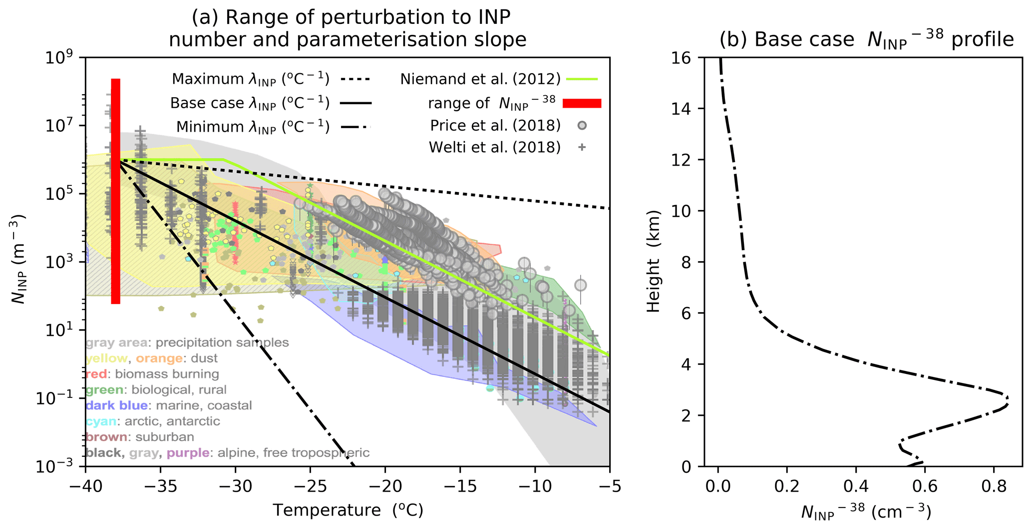
Figure 4 INP parameterisation slopes (λ_INP) and INP concentration profiles. The base case (black solid line), maximum/steepest (black dash-dotted line), and maximum/shallowest (black dashed line) perturbations to λ_INP are shown in panel (a) for an aerosol concentration of 1 cm⁻³ and a radius of 1 µm. The Niemand et al. (2012) parameterisation (light green solid line) is also shown. The INP parameterisations are overlain on Figs. 1–10 from Kanji et al. (2017) (©American Meteorological Society, used with permission), showing observed INP concentrations along with some recent measurements from Cabo Verde in grey (Price et al., 2018; Welti et al., 2018). Panel (b) shows the base case ${N_{\text{INP}}}^{-\mathrm{38}}$. Also shown in Fig. 1a is the range of ${N_{\text{INP}}}^{-\mathrm{38}}$ values (red bar), achieved by perturbing the profile shown in Fig. 1b. The range of ${N_{\text{INP}}}^{-\mathrm{38}}$ values shown by the red bar in Fig. 4a relate to the peak concentration shown in Fig. 4b at ∼ 3 km. Figure 4b shows the profile that the simulation was initiated with. The aerosols can be advected around, and the peak values shown in Fig. 4b are lifted to all cloud levels by the convective updraught (not shown).

2.2.1 Limiting INP number concentration (${N_{\text{INP}}}^{-\mathrm{38}}$)

The profile shown in Fig. 4b is the mean daily aerosol concentration, assumed to be predominately dust, in Cabo Verde extracted from a 2015 Global Model of Aerosol Processes (GLOMAP-mode; Mann et al., 2010) model simulation scaled to be approximately equal to the mean daily K-feldspar INP concentration from the same simulation (Vergara-Temprado et al., 2017). This is applied as the INP particle number concentration profile in the base case MONC–CASIM simulation. In the MONC model, INP is represented using the coarse mode dust aerosol. The uncertainty range of the ${N_{\text{INP}}}^{-\mathrm{38}}$ was defined by scaling the profile in Fig. 4b by a factor between 10⁻⁴ and 200, resulting in an ${N_{\text{INP}}}^{-\mathrm{38}}$ of between 8.4 × 10⁻³ and 168 cm⁻³. The range of ${N_{\text{INP}}}^{-\mathrm{38}}$ values of this study are shown in Fig. 4a (red bar), and the limits of this red bar correspond to the minimum and maximum values of observed INP from numerous collated field and laboratory measurements (Kanji et al., 2017). The values of ${N_{\text{INP}}}^{-\mathrm{38}}$ reported throughout the paper (i.e. in the range shown by the red bar in Fig. 4a and in all figures herein) relate to the ${N_{\text{INP}}}^{-\mathrm{38}}$ value at the peak of the aerosol layer in Fig. 4b (∼ 3 km). The strength of the warm bubble used to initiate the convection ensures that the aerosol concentration at lower altitude levels is transported to upper altitudes.

2.2.2 INP parameterisation slope (λ_INP)

λ_INP is defined as the change in the log ₁₀ of the INP number concentration per degree Celsius change in temperature as defined in Eq. (1):

$$\begin{array}{}\text{(1)}& {\mathit{\lambda }}_{\text{INP}}={\displaystyle \frac{\mathrm{d}\left({\log }_{\mathrm{10}}{N}_{\text{INP}}\right)}{\mathrm{d}\left(T\right)}}.\end{array}$$

where N_INP is the INP number concentration in m⁻³ and T is the temperature in degrees Celsius. Equation (1) is applied at temperatures between −38 and −3 ^∘C. The range of λ_INP values are calculated by varying the exponent (P, units of ${\mathrm{m}}^{-\mathrm{2}}{}^{\circ }{\mathrm{C}}^{-\mathrm{1}}$) in Eq. (2) below, which determines the number of active sites per unit area of an aerosol population at temperature T, from −1.3 and −0.1. For this study, we define the number of active sites, n_s, as

$$\begin{array}{}\text{(2)}& n_{\mathrm{s}}\left(T\right)=e^{PT+i},\end{array}$$

where i is the intercept of the natural logarithm of n_s (in active sites m⁻²) at 0 ^∘C and T is the ambient temperature in degrees Celsius. The equation is a basic form of n_s-based INP parameterisations and is adapted from Niemand et al. (2012). In the Niemand et al. (2012) parameterisation, P is −0.517 and results in a λ_INP of approx. −0.22 ${}^{\circ }{\mathrm{C}}^{-\mathrm{1}}$ for a dust concentration of 1 cm⁻³. This is shown as the base case λ_INP in Fig. 4a. The minimum (steepest) value of λ_INP is −0.5646 ${}^{\circ }{\mathrm{C}}^{-\mathrm{1}}$ (P = −1.3), which is slightly steeper than that of the Atkinson et al. (2013) parameterisation based on K-feldspar. The maximum (shallowest) value of λ_INP is −0.0434 ${}^{\circ }{\mathrm{C}}^{-\mathrm{1}}$ (P = −0.1), which is slightly shallower than that of the Meyers et al. (1992) parameterisation. The minimum (steepest) and maximum (shallowest) slopes simulated in this work are shown in Fig. 4a for a dust number concentration of 1 cm⁻³ with a mean radius of 1 µm. Using n_s(T), we can calculate the INP number concentration in m⁻³ at temperature T (${N_{\text{INP}}}^{\mathrm{T}}$) as follows:

$$\begin{array}{}\text{(3)}& {N_{\text{INP}}}^{\mathrm{T}}=min\left(n_{\mathrm{s}}\right(T)S,{N_{\text{INP}}}^{-\mathrm{38}}),\end{array}$$

where S is the surface area of the available INP in m² m⁻³ and ${N_{\text{INP}}}^{-\mathrm{38}}$ is the limiting INP number concentration in m⁻³ as defined in Sect. 2.2.1. The minimum function shown in Eq. (3) is not used in this paper at temperatures other than −38 ^∘C due to the parameterisation change described below.

Table 2 Experiment design. The base case, minimum, and maximum values of the variables perturbed in this study.

In addition to varying the exponent, the original Niemand et al. (2012) parameterisation is altered in this work to allow the intercept at 0 ^∘C to be flexible to ensure that the INP number concentration declines constantly from 0 to −38 ^∘C. This avoids interdependence between the ${N_{\text{INP}}}^{-\mathrm{38}}$ and λ_INP that can occur at low temperatures when the INP concentration plateaus between the warmest temperature where the parameterisation first predicts the temperature-dependent INP number concentration to be equal to the limiting INP number concentration and −38 ^∘C. This plateau can be seen in the Niemand et al. (2012) line in Fig. 4a and is discussed in Hawker et al. (2021). The decoupling of λ_INP and ${N_{\text{INP}}}^{-\mathrm{38}}$ was necessary to satisfy the assumptions of statistical emulation (Sect. 2.4) and to allow us to determine whether it is the limiting INP number concentration (e.g. total dust number concentration where dust is the only ice-nucleating material present in an aerosol population) or INP efficiency (e.g. whether the aerosol population is made up of marine organics or dust particles) that controls the properties of a deep convectively generated anvil cloud.

From Eqs. (2) and (3), we can see that

$$\begin{array}{}\text{(4)}& e^{PT+i}={\displaystyle \frac{{N_{\text{INP}}}^T}{S}}.\end{array}$$

Setting T to −38 ^∘C, the intercept (i in Eq. 2) of the INP parameterisation can be calculated as follows:

$$\begin{array}{}\text{(5)}& i=\ln \left({\displaystyle \frac{{N_{\text{INP}}}^{-\mathrm{38}}}{S}}\right)+\mathrm{38}P.\end{array}$$

2.2.3 The Hallett–Mossop process ice production efficiency (HM-eff)

The HM-eff in the model is varied from 1 to 1000 splinters produced per milligram of rimed liquid. The default efficiency of splinter production from the Hallett–Mossop process in MONC–CASIM is 350 mg⁻¹. This value is the best estimate of ice production based on a number of laboratory studies and has been used in previous modelling studies (Connolly et al., 2006; Hallett and Mossop, 1974; Mossop, 1985). However, other rates have been reported. An upper limit of 1000 mg⁻¹ aligns with previous modelling studies where the efficiency of ice production by the Hallett–Mossop process was varied (Connolly et al., 2006). This upper limit also allows us to account somewhat for the possibility that the Hallett–Mossop process operating in real clouds is stronger than that observed in laboratory studies (Field et al., 2017; Korolev et al., 2020; Takahashi et al., 1995).

2.3 Selection of uncertain input parameter combinations

MONC was run with combinations of values of ${N_{\text{INP}}}^{-\mathrm{38}}$, λ_INP, and HM-eff from within the ranges shown in Table 2. Combinations of parameter values were defined using a maximin Latin hypercube design algorithm. Latin hypercube sampling is based on the Latin square and ensures optimum space filling (Johnson et al., 2015; Lee et al., 2011; Mckay et al., 2000). The maximin algorithm maximises the minimum distance between points in the cube (Lee et al., 2011). The use of a maximin Latin hypercube sampling design means that the parameter combinations cover the three-dimensional parameter space in an optimum way. We can therefore evaluate the full effects of the parameters (individual and interacting) using traditional analysis on just the simulation data themselves, as well as employing statistical emulation (described in Sect. 2.4) to produce response surfaces of cloud properties.

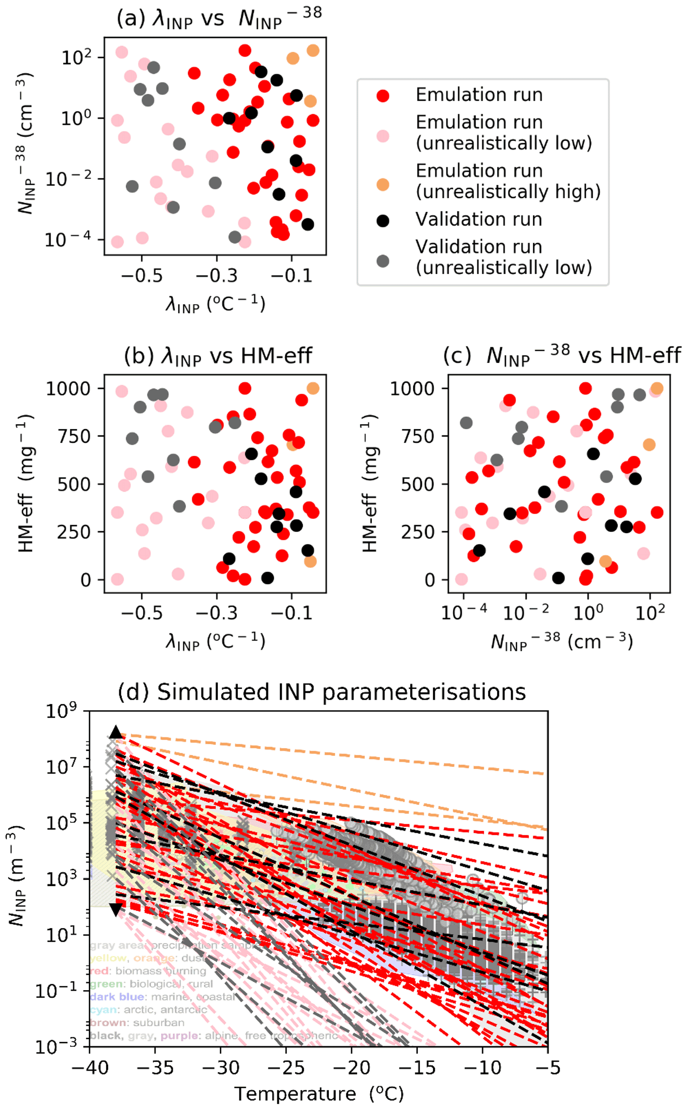
Figure 5 Experiment design. Values of the uncertain input parameter combinations used in the cloud model for the three uncertain input parameters (${N_{\text{INP}}}^{-\mathrm{38}}$ and λ_INP, a; λ_INP and HM-eff, b; and ${N_{\text{INP}}}^{-\mathrm{38}}$ and HM-eff, c). Shown in panel (d) is the resultant INP parameterisations arising due to the combination of perturbations to λ_INP and ${N_{\text{INP}}}^{-\mathrm{38}}$ overlain on Figs. 1–10 of Kanji et al. (2017) (©American Meteorological Society, used with permission). Output from the simulations shown in red, pink, and orange is used to build the emulator while output from the simulations shown in black or grey is used to validate the emulator results. The distinction between realistic (red, black) and unrealistic (pink, orange, grey) simulation perturbations is based on whether the corresponding parameterisation shown in panel (d) lies within the range of observations from Figs. 1–10 of Kanji et al. (2017).

The applied parameter values are shown in Fig. 5. In total 73 simulations of the deep convective cloud were carried out. The values of λ_INP and HM-eff were selected by sampling on a linear scale, while the values of ${N_{\text{INP}}}^{-\mathrm{38}}$ were selected by sampling on a logarithmic scale. This is because INP number concentrations vary over several orders of magnitude (Fig. 4a), and sampling ${N_{\text{INP}}}^{-\mathrm{38}}$ on a linear scale would bias the design to higher INP number concentrations.

The INP parameterisations corresponding to the ${N_{\text{INP}}}^{-\mathrm{38}}$ and λ_INP parameter values are shown in Fig. 5d. As a result of not representing the plateauing of the parameterisation (as can be seen in the Niemand et al., 2012, line in Fig. 4a) to avoid co-dependence between λ_INP and ${N_{\text{INP}}}^{-\mathrm{38}}$, a large part of the parameter space has unrealistically low INP concentrations (light grey and pink dots in Fig. 5a and light grey and pink lines in Fig. 5d). Additional simulations in the realistic regions of parameter space (shown by the red and black dots in Fig. 5a and red and black lines in Fig. 5d) were conducted to compensate for this, and the parameter combinations of the additional simulations were selected by augmenting points into the largest gaps in the realistic section of the original Latin hypercube design.

2.4 Statistical emulation of the model output

Statistical emulation is a “process by which the computer model is replaced by a statistical surrogate model that can be run more efficiently” (Lee et al., 2011). This approach has previously been used to look at deep convective cloud microphysical properties in a 3D model (Johnson et al., 2015), hail formation (Wellmann et al., 2018), nocturnal stratocumulus (Glassmeier et al., 2019), and aerosol forcing from volcanic eruptions (Marshall et al., 2019). In this study, as well as using traditional methods of analysis, we explore the usefulness of statistical emulation as a tool to understand the interacting effects of mixed-phase ice production mechanisms.

Statistical emulation (as well as the applied Latin hypercube sampling methodology) has advantages over traditional one-at-a-time tests (where one variable is varied at predictable values from a control or base case while all other variables are held constant). Firstly, it allows the exploration of the effects of simultaneously perturbing multiple uncertain input parameters on output variables of interest across the entirety of reasonable parameter space for a much reduced number of complex simulations. Secondly, dense sampling via statistical emulation enables techniques such as variance-based sensitivity analysis to be applied, through which we can identify the input parameters that are contributing the most uncertainty to important output responses. This subsequently allows for the direction of resources towards quantifying and accurately representing those key parameters that contribute large amounts of uncertainty to output variables of interest.

We use a Gaussian process as the basis for the emulator (Johnson et al., 2015; Lee et al., 2011; Marshall et al., 2019). A more detailed description of the process used to construct emulators can be found in Johnson et al. (2015) and Lee et al. (2011). Separate Gaussian process emulators are built from the output of the training simulations (i.e. the emulation runs shown in Fig. 5) for each of the target output variables listed in Table 1 using the statistical software R (R Core Team, 2017) and the DiceKriging package (Roustant et al., 2012). These emulators are 3D maps of how the values of the target output variables change in the simulation output depending on the three uncertain input parameters (Sect. 2.2); i.e. they are surrogate statistical representations of the MONC–CASIM model. The emulators assume a linear mean function including all uncertain inputs and a Matérn covariance structure. The Matérn covariance structure allows slightly more roughness in the output response than a pure Gaussian function (Rasmussen and Williams, 2006).

An underlying assumption of the Gaussian process emulator is that the output of the cloud model varies smoothly and continuously. Based on this assumption, the emulator fits a smooth response surface that passes directly through each training point. Techniques to allow extra noise in the output response, such as a variance nugget, were explored but were not used in the final emulator design as they did not substantially improve the emulator performance. To test whether the emulator can accurately predict the output of the cloud model, it is necessary to validate the prediction against output from simulations that have not been used to train the emulator. The simulations used to train and validate the emulator are shown in Fig. 5a–c. Fifty-two simulations are used to train each emulator. This is well in excess of the thirty simulations recommended by Loeppky et al. (2009), who states that 10 times the number of variable parameters is required. Eighteen simulations are used to validate the emulator. The model's output from these 18 simulations is compared with the mean and 95 % confidence interval predicted by the emulator at those combinations of the uncertain input parameters.

Variance-based sensitivity analysis is used to measure the sensitivity of the cloud model outputs to the three uncertain input parameters and their interaction effects (Johnson et al., 2015; Saltelli et al., 2000). The overall variance attributed to each input can be separated into the individual or main effect index of each input parameter and the total effect index which comprises the variation attributed to the input parameter in question itself and the variation due to interactions of that parameter with other input parameters (Saltelli et al., 2000). The main effect index of a parameter tells us the proportion of variance in the value of an output variable that could be minimised if the value of the given individual input parameter was known exactly. The difference between the total and main effect indices of a parameter tells us how much variance in the output variable is determined by the input parameter in question interacting with other input parameters (Johnson et al., 2015). In this work, the variance-based sensitivity analysis is carried out using the extended-FAST (Fourier amplitude sensitivity test) approach detailed in Saltelli et al. (1999).

3 Results

3.1 Anvil cloud properties

We first examine the effect of variations in ${N_{\text{INP}}}^{-\mathrm{38}}$, λ_INP, and HM-eff on anvil cloud properties. We focus on the anvil ice properties because the anvil cloud can persist in the atmosphere longer than the deep convective cloud that forms it (and beyond the simulation period presented here) and is therefore climatically important for cloud–radiation interactions. Tropical convectively produced cirrus can persist in the atmosphere for 1–2 d (Luo and Rossow, 2004) while the convective stage of the deep convective cloud simulated here has decayed after approximately 3 h. In Sect. 3.1.1 and 3.1.2, we examine the anvil ICNC and ice crystal size, respectively. An anvil with more numerous, smaller crystals will persist longer in the atmosphere than one with fewer, larger crystals. In Sect. 3.1.3, we examine the simulated anvil cloud fraction and the microphysical properties controlling it. The anvil region of the cloud is defined as the clouds occurring between 150 and 240 min in the simulations with a cloud base height greater than 9 km and an ice water path less than 0.04 kg m⁻². These quantities for specifying anvil cloud were based on qualitatively selecting the anvil region of the deep convective cloud by analysing a number of cloud properties. Other thresholds were tested, e.g. altitudes of 8–11 km, and did not change the results substantially or affect the qualitative findings in any meaningful way.

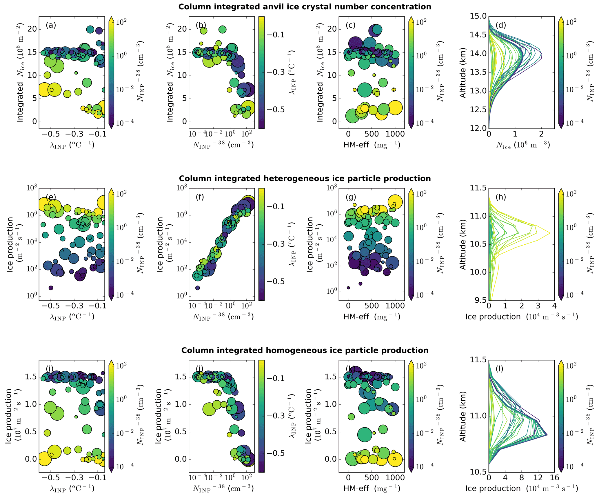
Figure 6 Anvil ICNC and ice particle production rates. Dependence of anvil ice crystal number concentration (a–d), ice particle production by heterogeneous freezing (e–h), and ice particle production by homogeneous freezing (i–l) on the three uncertain input parameters: λ_INP (a, e, and i), ${N_{\text{INP}}}^{-\mathrm{38}}$ (b, f, and j), and HM-eff (c, g, and k). In-cloud profiles of anvil ICNC (d), ice particle production by heterogeneous freezing (h), and ice particle production by homogeneous freezing (l) in all simulations coloured by ${N_{\text{INP}}}^{-\mathrm{38}}$. For panels (a), (e), and (i) the colour of the markers indicates ${N_{\text{INP}}}^{-\mathrm{38}}$ and the marker size indicates HM-eff. For panels (b), (f), and (j) the colour of the markers indicates λ_INP and the marker size indicates the HM-eff. For panels (c), (g), and (k) the colour of the markers indicates ${N_{\text{INP}}}^{-\mathrm{38}}$ and the marker size indicates the λ_INP value. Panels (a)–(d) are the average of the cloud property between 150 and 240 min (anvil stage) in the simulation, while panels (e)–(l) are the average of the relevant cloud property between 60 and 180 min (convective stage) in the simulations.

3.1.1 Anvil ice crystal number concentration

The column-integrated anvil ICNC from all simulations is shown in Fig. 6a–c. Figure 6d shows the associated mean anvil ICNC profile in each simulation. Anvil ICNCs are predominately controlled by the value of ${N_{\text{INP}}}^{-\mathrm{38}}$ (Fig. 6a–d), with a higher ${N_{\text{INP}}}^{-\mathrm{38}}$ causing lower anvil ICNCs at all altitudes (Fig. 6b and d). This is because the higher the ${N_{\text{INP}}}^{-\mathrm{38}}$, the higher the rate of heterogeneous freezing at the top of the mixed-phase cloud (Fig. 6e–h), reducing droplet transport to the homogeneous freezing regime and therefore homogeneous freezing rates (Fig. 6i–l). The homogeneous and heterogeneous ice particle production rates shown in Fig. 6e–l are the mean values from cloudy columns (Fig. 6e–g and i–k) or cloudy grid boxes (Fig. 6h and l) between 60 and 180 min of the simulation.

The INP parameterisation slope, λ_INP, plays a secondary role in controlling anvil ICNC (Fig. 6a). Simulations with a high ${N_{\text{INP}}}^{-\mathrm{38}}$ (yellow markers in Fig. 6a) have slightly lower anvil ICNC at shallow λ_INP. The chosen Hallett–Mossop splinter production efficiency has no notable impact on anvil ICNC regardless of the value of ${N_{\text{INP}}}^{-\mathrm{38}}$ or λ_INP.

Figure 7 Emulator validation and uncertain input contributions to output uncertainty. Validation of emulator results (a–c) and results of the variance-based sensitivity analysis (d–f) for anvil ICNC (a, b), ice particle production by heterogeneous freezing (c, d), and ice particle production by homogeneous freezing (e, f). In panels (a)–(c), the dots show the value of the validation run on the x axis and the corresponding emulator mean prediction on the y axis. The 95 % confidence intervals on the emulator predictions are also shown. An emulator that validates well will have dots close to the 1:1 line and small error bars. Panels (a) and (d) are the average of the cloud property between 150 and 240 min (anvil stage) of the simulation, while panels (b), (c), (e), and (f) are the average of the relevant cloud property between 60 and 180 min (convective stage) of the simulation.

We use statistical emulation to further examine the effects of our three uncertain input parameters (λ_INP, ${N_{\text{INP}}}^{-\mathrm{38}}$, HM-eff) on anvil ICNC and convective heterogeneous and homogeneous ice particle production. Figure 7a–c show a comparison of the output from the model validation simulations (shown in black and grey in Fig. 5a–d) with the corresponding emulator predictions for anvil ICNC and convective heterogeneous and homogeneous ice crystal number production, along with 95 % confidence intervals on the emulator predictions. All three outputs validate well with points close to or on the 1:1 line and small 95 % confidence intervals that overlap the 1:1 line most of the time. This indicates that the emulator can capture the variability in the idealised cloud model well for the output variables in question.

Figure 7d–f show the results of variance-based sensitivity analysis and indicate the relative importance of the uncertain input parameters in controlling the variance in the value of the output variable in question. As was inferred from Fig. 6, ${N_{\text{INP}}}^{-\mathrm{38}}$ is the dominant input parameter controlling the variance of anvil ICNC and heterogeneous and homogeneous ice particle production rates, while λ_INP and interaction effects contribute a non-negligible but secondary amount to the variance in anvil ICNC. Figure 7d indicates that ${N_{\text{INP}}}^{-\mathrm{38}}$ contributes to over 60 % of this output's variance. This means that the uncertainty in the exact value of the anvil ICNC could be significantly reduced if the value of ${N_{\text{INP}}}^{-\mathrm{38}}$ was to be known exactly. Similarly, this parameter is almost completely controlling the variance in the column-integrated heterogeneous ice particle production (Fig. 7e), with no real contribution from the other parameters here. Interaction effects account for up to 30 % of the variance in the anvil ICNC, indicating that the interaction between ${N_{\text{INP}}}^{-\mathrm{38}}$ and λ_INP is a substantial factor in determining the total number of ice crystals in a convectively generated anvil and may therefore affect the cloud lifetime.

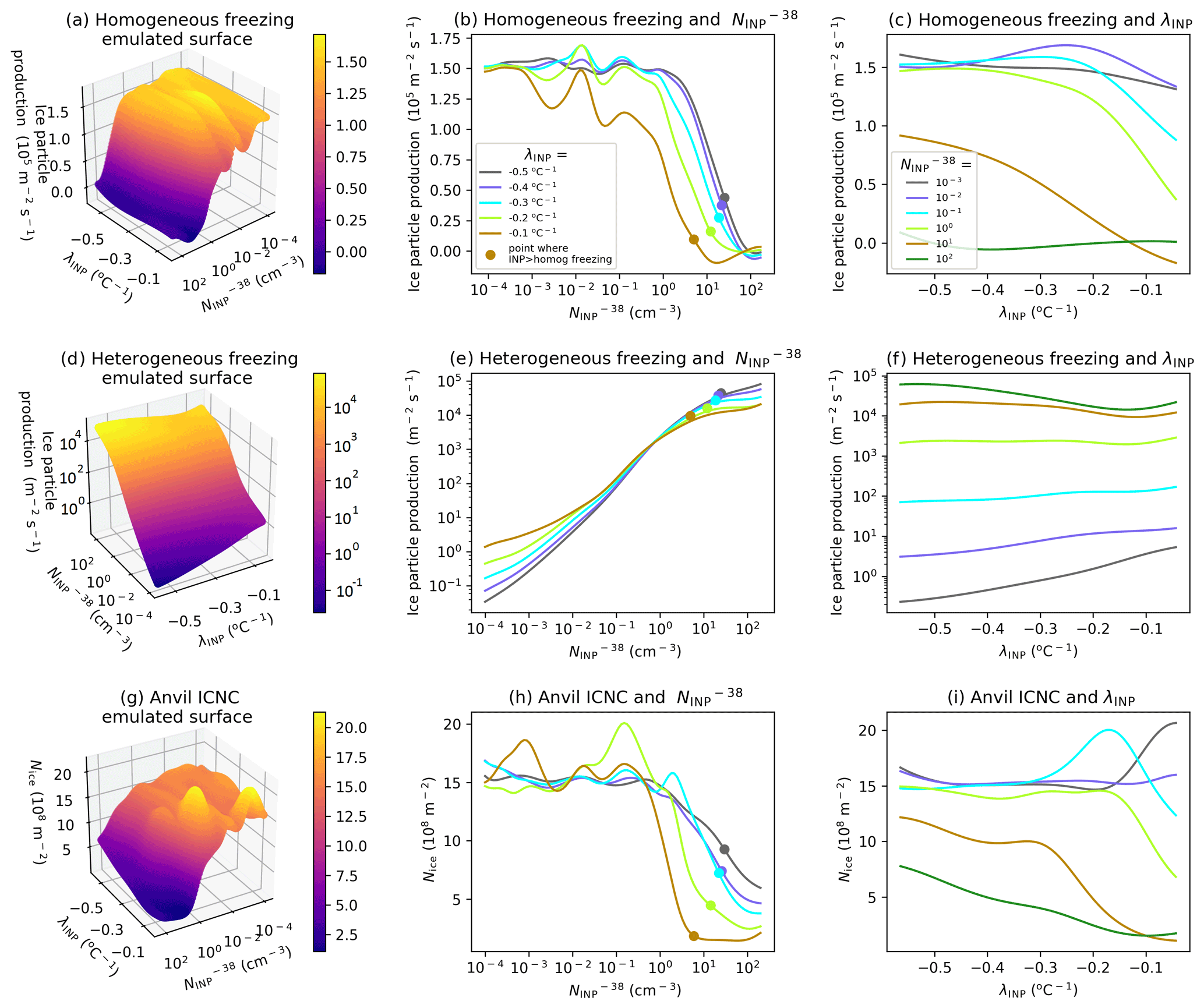
Figure 8 Emulator response surfaces. Prediction of ice particle production by homogeneous freezing (a–c), heterogeneous freezing (d–f), and anvil ICNC (g–i) by the emulator. Shown in panels (a), (d), and (g) are emulated response surfaces at a fixed HM-eff of 350 splinters produced per milligram of rimed liquid. The colours indicate output values and are the same range and units as the z axis. The line plots show the variation in predicted output value (y axis) from these response surfaces for fixed λ_INP (b, e, h) and fixed ${N_{\text{INP}}}^{-\mathrm{38}}$ (c, f, i). Panels (a)–(f) are the average of the cloud property between 60 and 180 min (convective stage) of the simulation, while panels (g)–(i) are the average of the relevant cloud property between 150 and 240 min (anvil stage) of the simulation.

Figure 8a, d, and g show the emulator surfaces for homogeneous (Fig. 8a) and heterogeneous (Fig. 8d) ice particle production and anvil ICNC (Fig. 8g) at a fixed HM-eff of 350 mg⁻¹. We hold the HM-eff constant because it had a minimal effect on the variance in the output variables (Fig. 7d–f); therefore, variations in its value do not alter the shape of the emulated surface substantially. It is important to note that the emulator response surface passes through each simulation point exactly, so it does not allow for noise on each point caused by internal variability of the cloud. As a result, the emulator surfaces should be interpreted by examining the general smoothly varying trends rather than individual bumps which may be an artefact of the emulator representing non-deterministic variations across the parameter space. Methods of smoothing the emulator surfaces could be explored in future studies (e.g. Marshall et al., 2019).

Ice particle production from homogeneous freezing is high and relatively constant between an ${N_{\text{INP}}}^{-\mathrm{38}}$ of 10⁻⁴ and 1 cm⁻³ before decreasing rapidly at higher ${N_{\text{INP}}}^{-\mathrm{38}}$ values (Fig. 8a). Meanwhile, ${N_{\text{INP}}}^{-\mathrm{38}}$ has the opposite effect on heterogeneous freezing, with heterogeneous ice particle production increasing relatively uniformly with increasing ${N_{\text{INP}}}^{-\mathrm{38}}$. This is because as more cloud liquid is consumed by heterogeneous freezing at mixed-phase levels due to droplet freezing and the associated increase in secondary ice production, riming, and deposition, fewer cloud droplets are available for homogeneous freezing.

Interaction between λ_INP and ${N_{\text{INP}}}^{-\mathrm{38}}$ freezing can be seen in the emulator response surfaces. At low ${N_{\text{INP}}}^{-\mathrm{38}}$, the heterogeneous ice particle production is highest for shallow-λ_INP values, while at high ${N_{\text{INP}}}^{-\mathrm{38}}$, the heterogeneous ice particle production rates are highest at steep λ_INP values (Fig. 8d). This is because at low ${N_{\text{INP}}}^{-\mathrm{38}}$ values, heterogeneous freezing at warm temperatures does not limit the number of cloud droplets reaching the upper mixed-phase region. However, at high ${N_{\text{INP}}}^{-\mathrm{38}}$, a shallow λ_INP inducing substantial freezing at warm temperatures will cause substantial cloud liquid consumption (by droplet freezing, secondary ice production, riming, and deposition) that will limit the availability of cloud droplets for heterogeneous freezing at colder mixed-phase levels. In Fig. 8g, we can see that when the ${N_{\text{INP}}}^{-\mathrm{38}}$ is high, the highest anvil ICNCs occur when the λ_INP is steep (between −0.3 and −0.5 ${}^{\circ }{\mathrm{C}}^{-\mathrm{1}}$). This is because at high-${N_{\text{INP}}}^{-\mathrm{38}}$ values, homogeneous freezing is very low and upper level mixed-phase heterogeneous freezing controls the anvil ICNC. At steep λ_INP values the consumption of cloud liquid at warm temperatures is lowest, leading to higher overall rates of heterogeneous freezing.

Figure 8b, e, and h show the mean emulator response across the uncertainty range of ${N_{\text{INP}}}^{-\mathrm{38}}$ of homogeneous (Fig. 8b) and heterogeneous (Fig. 8e) ice particle production and anvil ICNC (Fig. 8h) for different settings of λ_INP values (distinguished by line colours). The points on each line indicate the value of ${N_{\text{INP}}}^{-\mathrm{38}}$ at which the rate of ice particle production by heterogeneous freezing in the convective stage of the cloud development first exceeds that of homogeneous freezing. For all values of λ_INP, homogeneous ice particle production and anvil ICNC decline rapidly between ${N_{\text{INP}}}^{-\mathrm{38}}$ values of 1 and 100 as heterogeneous freezing approaches becoming, and subsequently becomes, the dominant mechanism for primary ice production. Homogeneous freezing is the dominant mechanism of ice crystal production at ${N_{\text{INP}}}^{-\mathrm{38}}$ < 10 cm⁻³ at all λ_INP values (Fig. 8b), above which heterogeneous freezing becomes the dominant mechanism of ice particle production (Fig. 8e). Homogeneous freezing is essentially completely shut off at ${N_{\text{INP}}}^{-\mathrm{38}}$ > 100 cm⁻³ (Fig. 8b), meaning that at very high ${N_{\text{INP}}}^{-\mathrm{38}}$ all primary ice crystals in the simulated deep convective cloud are formed via heterogeneous freezing. This is because heterogeneous freezing and subsequent processes in the mixed-phase region of the cloud significantly reduce the amount of cloud liquid reaching the homogeneous freezing altitude.

Anvil ICNC decreases sharply as INP concentration increases when heterogeneous freezing approaches becoming the dominant mechanism of primary cloud ice production (Fig. 8h). The exact point at which heterogeneous freezing becomes more powerful than homogeneous freezing depends on λ_INP, with the transition occurring at higher ${N_{\text{INP}}}^{-\mathrm{38}}$ values for a steep λ_INP. Consequently at high ${N_{\text{INP}}}^{-\mathrm{38}}$ (> 1 cm⁻³), the highest anvil ICNCs occur at steep λ_INP values, which allow more cloud droplets to reach the upper mixed-phase temperatures or the homogeneous freezing regime. Figure 8b, e, and h indicate that an INP number concentration of 1 cm⁻³ or more is enough to allow heterogeneous freezing to begin to compete with homogeneous freezing, while an INP number concentration of 100 cm⁻³ will shut off homogeneous freezing completely, regardless of λ_INP.

Figure 8c, f, and i show the mean emulator response across the uncertainty range of λ_INP of homogeneous (Fig. 8c) and heterogeneous (Fig. 8f) ice particle production and anvil ICNC (Fig. 8i) for different settings of ${N_{\text{INP}}}^{-\mathrm{38}}$ (distinguished by line colours). The ice particle production by homogeneous freezing is most sensitive to λ_INP at intermediate–high-${N_{\text{INP}}}^{-\mathrm{38}}$ values between 0.1 and 10 cm⁻³ where homogeneous freezing declines with increasing λ_INP (Fig. 8c). In particular, homogeneous ice particle production declines linearly with increasing λ_INP at a ${N_{\text{INP}}}^{-\mathrm{38}}$ of 10 cm⁻³. At an ${N_{\text{INP}}}^{-\mathrm{38}}$ of 100 cm⁻³, homogeneous freezing is completely shut down, and therefore there is no sensitivity to λ_INP evident in the emulator surface. Meanwhile, at a ${N_{\text{INP}}}^{-\mathrm{38}}$ of 10⁻³ cm⁻³, heterogeneous ice particle production is insufficient at all λ_INP values to affect homogeneous ice particle production, which remains uniformly high across the parameter space. Ice particle production by heterogeneous freezing is insensitive to changing λ_INP values except at the extremes of the ${N_{\text{INP}}}^{-\mathrm{38}}$ perturbations. There is a slight increase in heterogeneous ice particle production with increasing λ_INP at low ${N_{\text{INP}}}^{-\mathrm{38}}$ values and a slight decrease in heterogeneous ice particle production with decreasing λ_INP at high ${N_{\text{INP}}}^{-\mathrm{38}}$ (Fig. 8f). Anvil ICNC is sensitive to λ_INP values at high ${N_{\text{INP}}}^{-\mathrm{38}}$ (> 10 cm⁻³) where anvil ICNCs decline as λ_INP becomes more shallow (Fig. 8i) because shallow λ_INP can limit the number of cloud droplets available for low-temperature heterogeneous freezing (the main temperature region where ice crystals are formed in simulations with a high ${N_{\text{INP}}}^{-\mathrm{38}}$).

Overall anvil ICNC is controlled predominately by ${N_{\text{INP}}}^{-\mathrm{38}}$ with a secondary (but nonetheless important) effect from the INP parameterisation slope (λ_INP). The higher the ${N_{\text{INP}}}^{-\mathrm{38}}$, the lower the anvil ICNC. A shallow λ_INP can further reduce anvil ICNC, particularly at high-${N_{\text{INP}}}^{-\mathrm{38}}$ values. The anvil ICNC is reduced substantially when the number of heterogeneously frozen ice crystals exceeds the number of homogeneously frozen ice crystals due to the efficient consumption of liquid at upper mixed-phase cloud levels before droplets can be frozen homogeneously. The emulator response surfaces shown in Fig. 8 highlight the complex interactions between heterogeneous and homogeneous freezing and between heterogeneous freezing at different mixed-phase temperature levels (determined by the interaction between λ_INP and ${N_{\text{INP}}}^{-\mathrm{38}}$).

Figure 9 Anvil ice crystal size and driving processes. Dependence of anvil ice crystal effective radius (a–c), ice particle production by heterogeneous freezing between 5 and 7.5 km altitude (d–f), ice particle production by the Hallett–Mossop process (g–i), and the accretion of water by ice crystals (j–l) on the three uncertain input parameters: λ_INP (a, d, g, j), ${N_{\text{INP}}}^{-\mathrm{38}}$ (b, e, h, k), and HM-eff (c, f, i, l). For the leftmost column, the colour of the markers indicates ${N_{\text{INP}}}^{-\mathrm{38}}$ and the marker size indicates HM-eff. For the middle column, the colour of the markers indicates λ_INP and the marker size indicates the HM-eff. For the rightmost column, the colour of the markers indicates ${N_{\text{INP}}}^{-\mathrm{38}}$ and the marker size indicates λ_INP. Panels (a)–(c) are the average of the cloud property between 150 and 240 min (anvil stage) in the simulation, while panels (d)–(l) are the average of the relevant cloud property between 60 and 180 min (convective stage) in the simulations. Note that panels (d)–(f) differ from Fig. 6e–g because of the different altitudes: Figure 6 shows the total column-integrated heterogeneous ice particle production, while Fig. 9 (here) shows only the heterogeneous ice particle production occurring in the Hallett–Mossop region (5–7.5 km).

3.1.2 Anvil ice crystal size

We now examine how ${N_{\text{INP}}}^{-\mathrm{38}}$, λ_INP, and HM-eff affect the anvil ice crystal size. The measure we use to quantify ice crystal size is the effective radius or the ratio of the third to the second moments of the ice crystal size distribution. A larger ice crystal size indicates that anvil ice particles will have lower scattering potential (much like the Twomey effect for cloud droplets). A larger ice crystal size also indicates higher fall speeds and lower lifetimes, theoretically reducing the lifetime of the anvil cloud and reducing its radiative effect. The simulated ice crystal effective radius in the anvil cloud region at 14 km can be seen in Fig. 9a–c. We used the effective radius at 14 km because 14 km is the altitude of peak ICNC shown in Fig. 6d.

Anvil ice crystal effective radius exhibits two distinct regimes depending on the value of λ_INP, which can be seen in Fig. 9a and b. Simulations with a λ_INP shallower (larger) than approximately −0.3 ${}^{\circ }{\mathrm{C}}^{-\mathrm{1}}$ (Fig. 9a) exhibit a large jump from under 25 µm and very little variation between simulations to over 27 µm, with a large spread in ice crystal effective radius between simulations. In simulations with a shallow λ_INP and an effective radius greater than 27 µm, the value of the effective radius is dependent on the ${N_{\text{INP}}}^{-\mathrm{38}}$, with simulations with larger ${N_{\text{INP}}}^{-\mathrm{38}}$ values having a larger ice crystal size (Fig. 9b). This indicates that while anvil ICNC was determined predominately by ${N_{\text{INP}}}^{-\mathrm{38}}$ with λ_INP having a secondary role, ice crystal size is determined predominately by λ_INP with ${N_{\text{INP}}}^{-\mathrm{38}}$ having a secondary role. This is because ice crystal size is more strongly affected than ICNC by the altitude of ice formation, the amount of liquid available for riming, and the time available for deposition growth. Therefore, ice crystal effective radius is predominately affected by INP number concentration at warm temperatures where liquid is available for ice crystal growth which is determined by λ_INP.

The mechanism for the increased ice crystal size at shallow-λ_INP and high-${N_{\text{INP}}}^{-\mathrm{38}}$ values is as follows: ice crystals in clouds with a shallower λ_INP values have larger concentrations of heterogeneously frozen crystals at warm mixed-phase temperatures (Fig. 9d–f). This increase in heterogeneously frozen ice crystals in the Hallett–Mossop region leads to an increase in ice particle production by the Hallett–Mossop process (Fig. 9g–i). We see a large increase of approximately 1 order of magnitude in ice particle production by the Hallett–Mossop process at shallow λ_INP (Fig. 9g) and a bifurcation in cloud behaviour because of this enhancement. The output data are split into two populations, or regimes, based on the λ_INP value, with ice effective radius in each regime having a linear dependence on HM-eff (Fig. 9i). Within the warmer temperature mixed-phase cloud region, liquid is still available when crystals are frozen for riming. Therefore, with more heterogeneously frozen ice crystals at lower cloud altitudes, there are higher riming rates (Fig. 9j–l), more ice crystal growth, and overall larger ice crystal sizes.

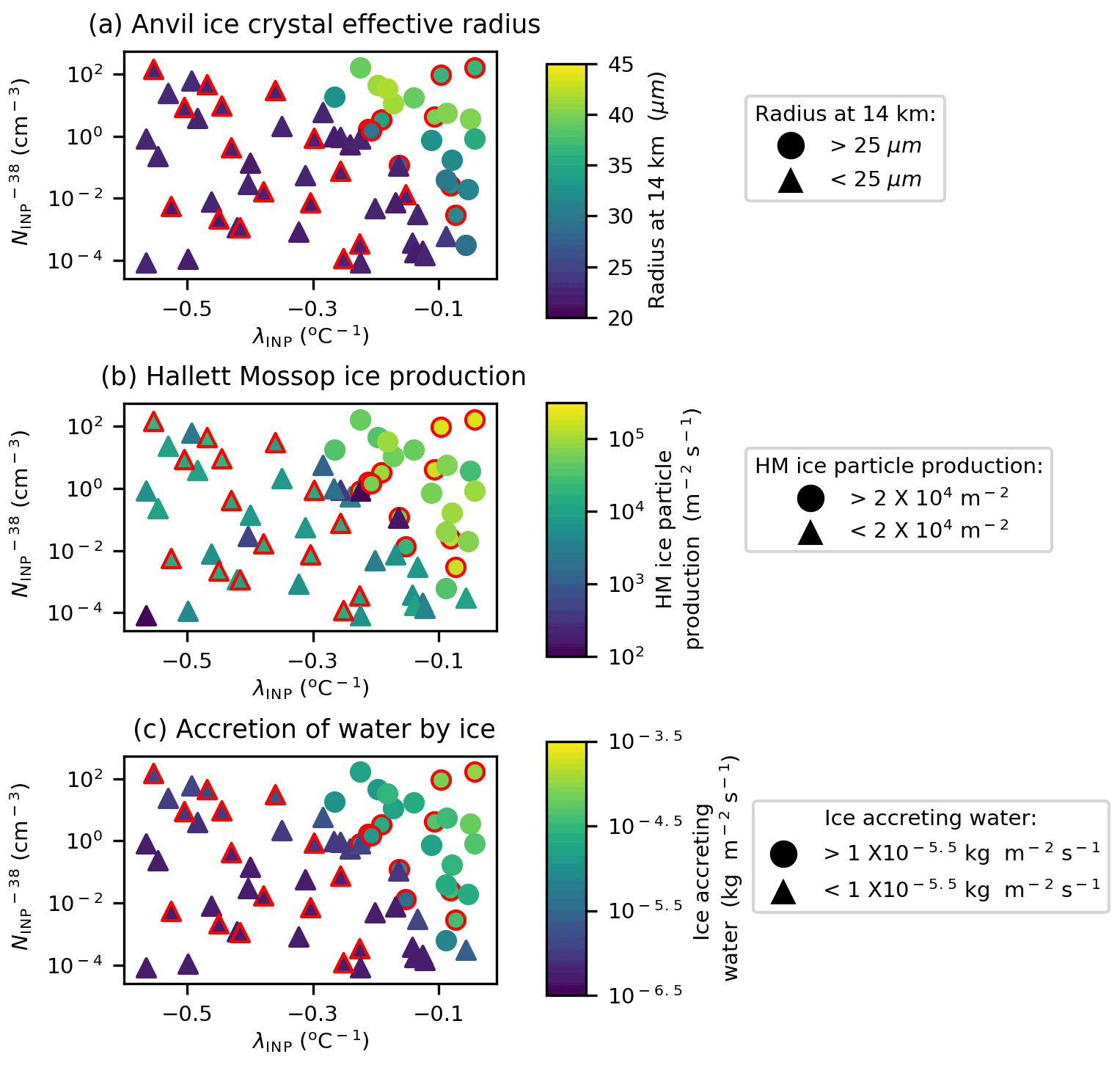
Figure 10 Regime change in anvil ice crystal effective radius and driving processes. Variation in anvil ice crystal effective radius (a), ice particle production by the Hallett–Mossop process (b), and the accretion of water by ice crystals (c) due to variation in λ_INP and ${N_{\text{INP}}}^{-\mathrm{38}}$. Marker colours indicate the value of anvil ice crystal effective radius (a), ice particle production by the Hallett–Mossop process (b), and the accretion of water by ice crystals (c). Circular markers indicate an ice crystal effective radius above 25 µm (a), an ice particle production by Hallett–Mossop exceeding 2 × 10⁴ ${\mathrm{m}}^{-\mathrm{2}}{\mathrm{s}}^{-\mathrm{1}}$ (b), and a rate of water accretion by ice over 1 × 10^−5.5 $\mathrm{kg}{\mathrm{m}}^{-\mathrm{2}}{\mathrm{s}}^{-\mathrm{1}}$ (c). Simulations with a HM-eff above 600 splinters mg⁻¹ are indicated with a red outline. Panel (a) is the average of the cloud property between 150 and 240 min (anvil stage) of the simulation, while panels (b) and (c) are the average of the relevant cloud property between 60 and 180 min (convective stage) of the simulation.

Figure 9a, g, and j illustrate a regime change at shallow-λ_INP values with large increases in anvil ice crystal size (Fig. 9a), Hallett–Mossop ice particle production (Fig. 9g), and accretion of water by ice (Fig. 9j) at values of λ_INP above approximately −0.3 ${}^{\circ }{\mathrm{C}}^{-\mathrm{1}}$. This regime change is further illustrated in Fig. 10, which shows the variation in anvil ice crystal effective radius (Fig. 10a), convective Hallett–Mossop ice particle production (Fig. 10b), and accretion of water by ice (Fig. 10c) with changing λ_INP and ${N_{\text{INP}}}^{-\mathrm{38}}$ values. The value of all three output variables substantially increases in the upper right corner of all three panels of Fig. 10, corresponding to shallow-λ_INP and high-${N_{\text{INP}}}^{-\mathrm{38}}$ values. The ${N_{\text{INP}}}^{-\mathrm{38}}$ determines at what λ_INP the regime change occurs: at an ${N_{\text{INP}}}^{-\mathrm{38}}$ of ∼ 10⁻⁴ cm⁻³, λ_INP must be greater than −0.1 ${}^{\circ }{\mathrm{C}}^{-\mathrm{1}}$ for the regime change to occur. At an ${N_{\text{INP}}}^{-\mathrm{38}}$ greater than 10 cm⁻³, the regime change occurs when λ_INP is greater than −0.3 ${}^{\circ }{\mathrm{C}}^{-\mathrm{1}}$. The regime change occurs in the same location of parameter space in all three variables (Fig. 10). Simulations in the shallow-λ_INP regime with a HM-eff above 600 mg⁻¹ are highlighted with a red outline, and the lack of distinction in colour between simulations with a high HM-eff in the low ${N_{\text{INP}}}^{-\mathrm{38}}$ and steep λ_INP regions indicates that a high HM-eff does not have the same effect in the cloud as a shallow λ_INP; i.e. simulations with a steep λ_INP and high HM-eff cannot experience the same elevated Hallett–Mossop ice particle production, accretion rates, and resultant increase in the anvil ice crystal effective radius as a simulation with a shallow λ_INP and a low HM-eff. However, simulations on the border of the regime transition seem more likely to have elevated ice effective radius and thus be in the shallow-λ_INP regime if they have a high HM-eff.

Figure 11 Emulator validation and uncertain input contributions to output uncertainty. Validation of emulator results (a–c) and results of the variance-based sensitivity analysis (d–f) for anvil effective radius at 14 km (a, b), ice particle production by the Hallett–Mossop process (c, d), and water accretion by ice (e, f). In panels (a)–(c) the dots show the value of the validation run on the x axis and the corresponding emulator mean prediction on the y axis. The 95 % confidence intervals of the emulator mean predictions are also shown. An emulator that validates well will have dots close to the 1:1 line and small error bars. Panels (a) and (d) are the average of the cloud property between 150 and 240 min (anvil stage) of the simulation, while panels (b), (c), (e), and (f) are the average of the relevant cloud property between 60 and 180 min (convective stage) of the simulation.

Statistical emulation of anvil ice crystal effective radius at 14 km, Hallett–Mossop ice particle production, and accretion of water by ice crystals was attempted. Figure 11a–c show the validation of the emulator surface against the cloud model validation points. In all three cases the emulator does not validate as well as was seen in Fig. 7 with larger 95 % confidence intervals. Applying a nugget, a term to introduce noise, to allow the emulator to pass nearby to, rather than directly through, the training points (Johnson et al., 2011) was tested as a means to improve the validation. However, because the poorer validation occurs mainly as a result of the emulator struggling with the sharp transitions at shallow-λ_INP values seen in Fig. 9a, g, and j, a nugget term did not change the results. Nevertheless, in most cases the points are relatively close to the 1:1 line, indicating that the emulator has some skill in predicting ice crystal size and the cloud development properties that control ice crystal size.

Figure 11d–f show the results of variance-based sensitivity analysis and indicate that for all three output variables considered here, λ_INP accounts for a large proportion of the variance with a main effect index of 30 % to 60 %. Interaction effects between the λ_INP and the ${N_{\text{INP}}}^{-\mathrm{38}}$ account for around 20 % of the variance in the anvil ice crystal size. The variance in the anvil ice crystal size and the accretion of water by ice of the simulated cloud would be substantially reduced by knowing the values of λ_INP and ${N_{\text{INP}}}^{-\mathrm{38}}$ exactly, while the variance in the ice particle production by the Hallett–Mossop process would be substantially reduced by knowing the values of λ_INP and HM-eff exactly.

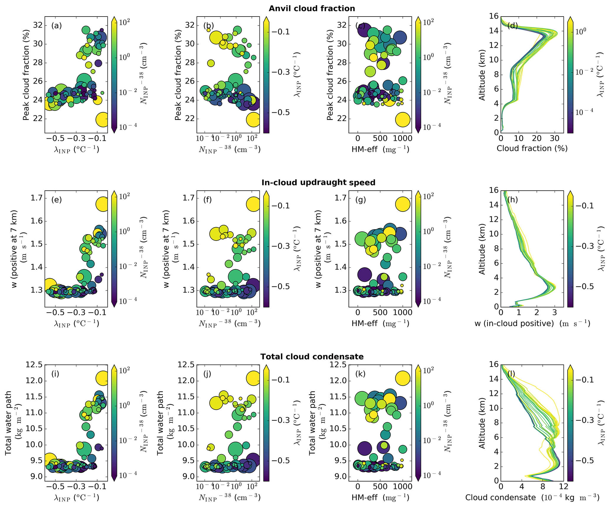
Figure 12 Anvil cloud fraction and driving processes. Dependence of anvil cloud fraction (a–d), in-cloud updraught speed at 7 km (e–h), and total cloud condensate (i–l) on the three uncertain input parameters: λ_INP (a, e, i), ${N_{\text{INP}}}^{-\mathrm{38}}$ (b, f, j), and HM-eff (c, g, k). In-cloud profiles of anvil cloud fraction (d), in-cloud updraught speed (h), and total cloud condensate (l) in all simulations are coloured by λ_INP. For panels (a), (e), and (i) the colour of the markers indicates ${N_{\text{INP}}}^{-\mathrm{38}}$ and the marker size indicates the HM-eff. For panels (b), (f), and (j) the colour of the markers indicates λ_INP and the marker size indicates HM-eff. For panels (c), (g), and (k) the colour of the markers indicates ${N_{\text{INP}}}^{-\mathrm{38}}$ and the marker size indicates λ_INP. Panels (a)–(d) are the average of the cloud property between 150 and 240 min (anvil stage) in the simulation, while panels (e)–(l) are the average of the relevant cloud property between 60 and 180 min (convective stage) in the simulations.

Appendix Fig. A1 shows emulator response surfaces for anvil ice crystal effective radius at 14 km (Fig. A1a), ice particle production by the Hallett–Mossop process (Fig. A1b), and accretion of water by ice crystals (Fig. A1c). In Fig. A1a and c, the Hallett–Mossop splinter production efficiency is held constant at 350 splinters produced per milligram of rimed liquid. In Fig. A1b, ${N_{\text{INP}}}^{-\mathrm{38}}$ is held constant at 1 cm⁻³. The emulator response surfaces are noisier, with more bumps than those shown in Fig. 8. This is expected due to the larger 95 % confidence intervals on the emulator predictions shown in Fig. 11a–c. Emulation using a Gaussian process assumes that the uncertain input parameters cause changes in output variables that vary smoothly over the parameter space. This is not the case for the three variables emulated in Fig. 12. For example, ice particle production by the Hallett–Mossop process shows a distinct regime change at shallow-λ_INP values, with a sharp upwards bend in the emulator surface occurring at a λ_INP of approximately −0.2 ${}^{\circ }{\mathrm{C}}^{-\mathrm{1}}$ (Fig. A1b). However, in general the response surfaces represent the trends seen in Figs. 9 and 10 reasonably well. For example, the emulated response surfaces show increases with high-${N_{\text{INP}}}^{-\mathrm{38}}$ and shallow-λ_INP values that are also evident in Figs. 9 and 10.

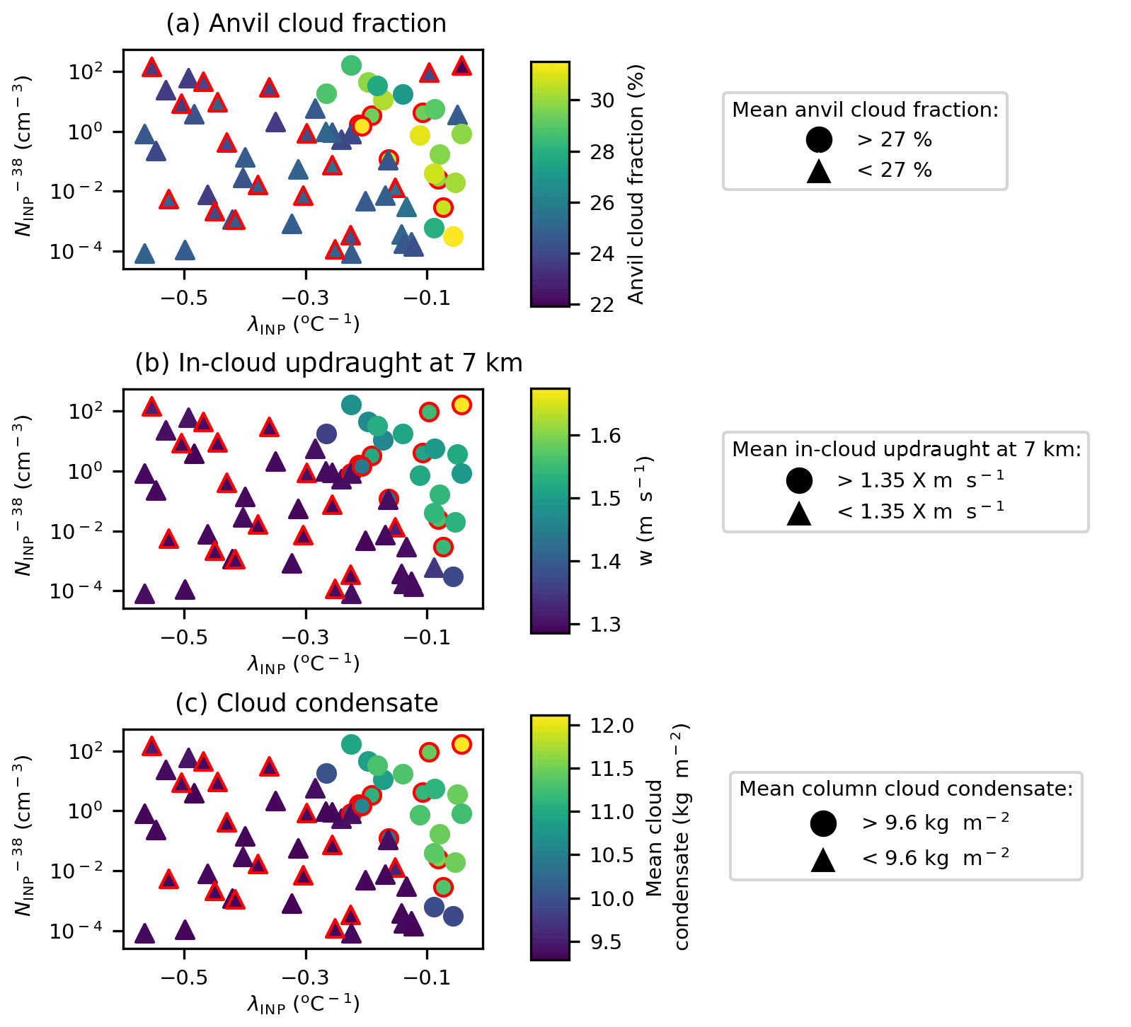
Figure 13 Regime change in anvil cloud fraction and driving processes. Variation in anvil cloud fraction (a), in-cloud updraught speed at 7 km (b), and total cloud water path (c) due to variation in λ_INP and ${N_{\text{INP}}}^{-\mathrm{38}}$. Marker colours indicate the value of the mean peak anvil cloud fraction (a), in-cloud updraught speed at 7 km (b), and total cloud water path (c). Circular markers indicate a cloud fraction above 27 % (a), a mean in-cloud updraught speed above 1.35 m s⁻¹ (b), and a water path over 9.6 kg m⁻² (c). Simulations with a HM-eff above 600 splinters mg⁻¹ are indicated with a red outline. Panel (a) is the average of the cloud property between 150 and 240 min (anvil stage) of the simulation, while panels (b) and (c) are the average of the relevant cloud property between 60 and 180 min (convective stage) of the simulation.

3.1.3 Anvil cloud fraction

Figure 12 shows the dependence of anvil cloud fraction (Fig. 12a–d), in-cloud updraught speed (Fig. 12e–h), and total cloud condensate amount (Fig. 12i–l) on the uncertain input parameters. The mean cloud fraction profile occurring between 180 and 240 min of the simulations is shown in Fig. 12d. The anvil cloud fraction values shown in Fig. 12a–c, and used in all further analysis of the anvil cloud fraction, are the peak values of the profile shown in Fig. 12d. A similar regime shift at shallow-λ_INP values as was seen in the anvil ice crystal size is seen in all three of the output variables considered here (Fig. 12a, e, and i): simulations with a shallow λ_INP (>−0.3 ${}^{\circ }{\mathrm{C}}^{-\mathrm{1}}$) have a higher cloud fraction, with the exception of two outlier simulations with very high ${N_{\text{INP}}}^{-\mathrm{38}}$ and shallow λ_INP which have very low cloud fractions. A small secondary dependence of cloud fraction on ${N_{\text{INP}}}^{-\mathrm{38}}$ is evident with simulations in the shallow-λ_INP regime, exhibiting reductions in cloud fraction from ∼ 32 % at low ${N_{\text{INP}}}^{-\mathrm{38}}$ values to ∼ 28 % at higher ${N_{\text{INP}}}^{-\mathrm{38}}$ values. The regime shift to high cloud fractions, updraught speed, and cloud condensate occurs in the same shallow-λ_INP and high-${N_{\text{INP}}}^{-\mathrm{38}}$ region of parameter space (Fig. 13) as was anvil ice crystal size, Hallett–Mossop ice particle production, and ice accretion rates (Fig. 10).

Anvil cloud fraction is enhanced at shallow-λ_INP values due to an invigoration effect caused by enhanced heterogeneous (Fig. 9d–f) and secondary freezing (Fig. 9g–i) and increased riming (Fig. 9j–l) in the mixed-phase cloud region, as well as the resultant enhancement in latent heat release, updraught speeds (Fig. 12e and h), and vertical condensate mass transport (Fig. 12i and l). Increased ice crystal sizes at shallow-λ_INP values in the convectively generated anvil discussed in Sect. 3.1.2 (Figs. 9–12) would be expected to reduce anvil size, due to the associated increases in ice fall speed. Within the time period analysed here, the enhancement in convective strength (inferred from enhanced updraught speeds) and the resultant increase in anvil size at shallow-λ_INP values compensate for the effect of increased anvil ice crystal size. The importance of the anvil ice crystal properties relative to the convective invigoration effect for anvil cloud fraction may change with a longer simulation period owing to the persistence of the anvil cloud after the decay of the convection that forms it, and this should be examined in future studies.

The small reduction of anvil cloud fraction within the shallow-λ_INP regime with increasing ${N_{\text{INP}}}^{-\mathrm{38}}$ (Fig. 12b) can be attributed to the changes in anvil ice crystal properties reported in Sect. 3.1.1 and 3.1.2. At high-${N_{\text{INP}}}^{-\mathrm{38}}$ values, ICNC is reduced (Fig. 6b) and ice crystal size is increased (Fig. 9b). Fewer and larger crystals will sediment out faster and therefore will spread out over a smaller horizontal area, reducing anvil fraction in simulations with high-${N_{\text{INP}}}^{-\mathrm{38}}$ values. The chosen Hallett–Mossop splinter production efficiency has very little impact on anvil cloud fraction (Fig. 12c), updraught speeds (Fig. 12g), or cloud condensate amount (Fig. 12k).

Emulation of anvil cloud fraction was attempted but, the bifurcation of these output data into the two distinct regimes depending on the value of λ_INP proved impossible to capture with our emulator approach, and validation of the emulation showed little predictive power (not shown). Recently developed emulator approaches that attempt to overcome the smoothness assumption of the Gaussian process emulator used here could be explored in future studies (Pope et al., 2021; Volodina and Williamson, 2020). This indicates that although emulation is a powerful tool to aid in our understanding of cloud processes, traditional methods of analysis are also still needed where there are complex sharp transitions such as those seen in Fig. 13. It is not clear why the emulation of some variables with two distinct regimes (such as ice crystal effective radius) worked relatively well and emulation of anvil cloud fraction did not.

3.2 The importance of the Hallett–Mossop process and its interaction with λ_INP

One notable feature of the results presented so far is the apparent insensitivity of most cloud properties to the HM-eff. For example, the results of the variance-based sensitivity analysis shown in Figs. 7 and 11 indicate that the HM-eff makes no significant contribution to the uncertainty in the value of anvil ICNC, heterogeneous or homogeneous freezing rates, anvil effective radius, or ice accretion of water. Ice particle production by the Hallett–Mossop process was the only output variable shown to have a notable dependence on the HM-eff, and up to 40 % of the uncertainty in its value was attributed to variation in the λ_INP value owing to the role of λ_INP in determining the regime shift evident in Figs. 9g and 10b. This regime shift induces an enhancement in the ice particle production by the Hallett–Mossop process of about 1 order of magnitude at shallow-λ_INP values regardless of the value of HM-eff by increasing the number of primary ice crystals available to initiate the Hallett–Mossop process.

Figure 14 Importance of ice production in the Hallett–Mossop ice production regime (5–7.5 km). Dependence of cloud properties on ice particle production in the Hallett–Mossop regime (5–7.5 km) in the convective stage of cloud development (60–180 min). Shown is ICNC at 7 km (a); column cloud droplet number concentration (b); accretion of water by ice (c); graupel mass (d); snow mass (e); in-cloud updraught speed at 7 km (f); cloud condensate from cloud droplets, rain, ice crystals, snow, and graupel (g); anvil ice crystal effective radius at 14 km (h); and anvil cloud fraction (i). The colour of the markers indicates λ_INP and the marker size indicates the HM-eff. Panels (a)–(g) are the average of the cloud property between 60 and 180 min (convective stage) of the simulation, while panels (h)–(i) are the average of the relevant cloud property between 150 and 240 min (anvil stage) of the simulation. Simulations deemed as having unrealistically high or unrealistically low INP concentrations due to the combined perturbations of λ_INP and ${N_{\text{INP}}}^{-\mathrm{38}}$ (as indicated in Fig. 5) are not shown in this plot or included in the correlation analysis.

In most simulations, over 99 % of ice crystals in the Hallett–Mossop region (5–7.5 km) are formed via the Hallett–Mossop process and not via heterogeneous ice formation (Fig. A2). Figure A2 shows that only 7 of 73 simulations have more than 10 % of the ice particle production between 5 and 7.5 km occurring via heterogeneous ice nucleation rather than via the Hallett–Mossop process. Many output variables, particularly those exhibiting a regime shift at shallow λ_INP and high ${N_{\text{INP}}}^{-\mathrm{38}}$, show a strong correlation with ice particle production in the Hallett–Mossop region of the cloud (Fig. 14). This is in spite of the apparent unimportance of the chosen HM-eff for the simulated cloud properties detailed in Sect. 3.1. This correlation indicates that the key role of the INP slope in determining cloud properties can be partly attributed to its role in enhancing Hallett–Mossop ice particle production rates (Fig. 9g–i), which dominate ice production in the Hallett–Mossop regime (Appendix Fig. A1). To avoid biasing the correlation analysis to simulations with unrealistically low concentrations of INP in the Hallett–Mossop regime which have very low variability between simulations, the simulations and correlation analysis shown Fig. 14 comprise only simulations from the realistic region of parameter space (Fig. 5).

Ice particle production by the Hallett–Mossop process is greatly enhanced at shallow-λ_INP values due to both the larger availability of seed ice crystals and the enhanced riming that accompany these increased ICNCs. This indicates that INP particles can exert strong control over deep convective cloud properties even when heterogeneous freezing is not the dominant mechanism of ice production because they can alter the rate of ice production by SIP mechanisms (Figs. 9g, 14, and A1).

In particular, we note that high rates of ice particle production by the Hallett–Mossop process do not occur unless the λ_INP is shallow. This is evident from the lack of distinction between simulations with a HM-eff above or below 600 splinters mg⁻¹ in Figs. 10 and 14 (compare simulations shown with and without a red outline). This indicates that a steep λ_INP and a high HM-eff cannot have the same effect on the cloud properties as a shallow λ_INP regardless of the HM-eff. Furthermore, ICNCs at lower mixed-phase altitudes, regardless of the freezing mechanism in question, can be key determinants of deep convective cloud properties and the properties of the convectively generated anvil (Fig. 14).

Figure 14 indicates that as ice production by the Hallett–Mossop process increases due to increased INP number concentrations at shallow-λ_INP values, mixed-phase ICNCs (Fig. 14a) are increased and column cloud droplet number concentrations are reduced (Fig. 14b). Due to the enhancement in ICNC in the lower mixed-phase region with shallower λ_INP and higher resultant Hallett–Mossop ice particle production, increases are seen in all mixed-phase freezing mechanisms including accretion of water by ice (Fig. 14c), as well as column graupel (Fig. 14d) and snow (Fig. 14e) mass concentrations due to the well-documented enhanced effectiveness of liquid collection by frozen hydrometeors relative to liquid ones (Johnson, 1987; Phillips et al., 2005). Enhanced latent heat release by the increased freezing events from multiple pathways leads to increased updraught speeds (Fig. 14f) and an overall increase in cloud formation (Fig. 14g). Enhanced riming in the mixed-phase region increases anvil ice crystal effective radius (Fig. 14h) as more anvil ice crystals are formed via heterogeneous freezing and are subject to riming than are formed via homogeneous freezing. The increased convective strength also leads to increased anvil cloud fraction (Fig. 14i).

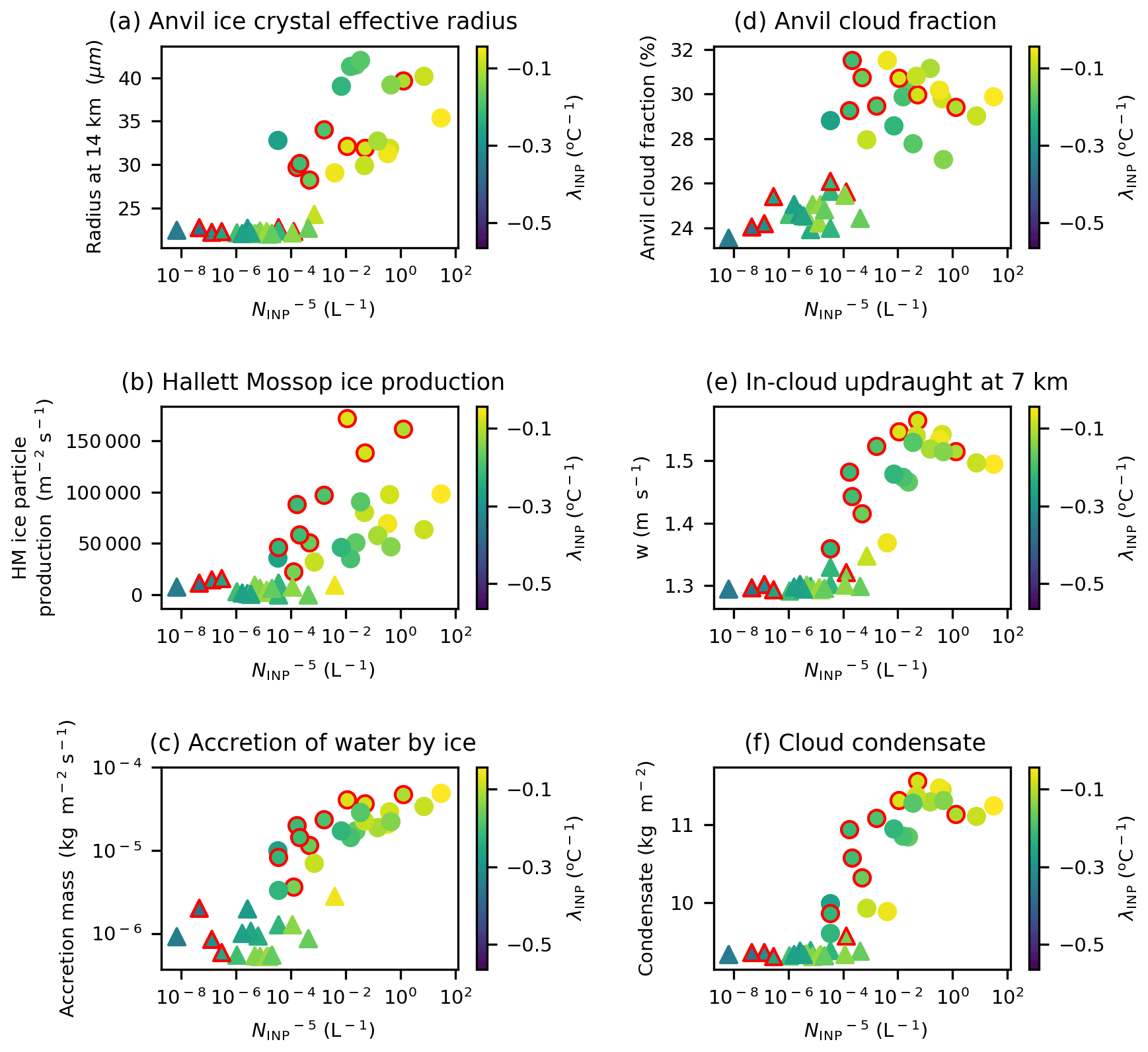
Figure 15 INP concentrations in the Hallett–Mossop regime and related key cloud properties. INP number concentrations at −5 ^∘C and anvil ice crystal size (a), ice particle production by the Hallett–Mossop process (b), accretion of water mass by ice crystals (c), anvil cloud fraction (d) in-cloud updraught speed at 7 km (e), and mean column cloud condensate mass (f). The marker colour is determined by the λ_INP. The thresholds between triangular and circular markers are determined by the regime changes identified previously in Figs. 10 and 14. Simulations with a HM-eff above 600 splinters mg⁻¹ are indicated with a red outline. Panels (a) and (d) are the average of the cloud property between 60 and 180 min (convective stage), while panels (b), (c), (e), and (f) are the average of the relevant cloud property between 150 and 240 min (anvil stage) of the simulation.

Many studies have tried to establish a threshold concentration of INP where significant Hallett–Mossop ice production begins to occur and affect cloud properties (e.g. Crawford et al., 2012; Huang et al., 2017). Figure 15 compares the INP number concentration at −5 ^∘C ($N_{\text{INP}}^{-\mathrm{5}}$) extracted from Fig. 5d (i.e. within the Hallett–Mossop region) to the anvil ice crystal size (Fig. 15a), the Hallett–Mossop ice particle production (Fig. 15b), the accretion of water by ice (Fig. 16c), the anvil cloud fraction (Fig. 15d), the updraught speed at 7 km (Fig.16e), and the total column condensate (Fig. 15f). We can see that there is little variation in the cloud properties shown below an $N_{\text{INP}}^{-\mathrm{5}}$ of 10⁻⁵ L⁻¹. Above this INP concentration, there is an increase in all properties shown. Simulations with HM-eff values above 600 splinters mg⁻¹ generally show an enhancement in Hallett–Mossop ice particle production (Fig. 15b), accretion (Fig. 15c), invigoration (Fig. 15e), and cloud condensate (Fig. 15f) at lower Hallett–Mossop regime INP concentrations than simulations with lower HM-eff values (compare markers with red outline to markers without an outline at similar $N_{\text{INP}}^{-\mathrm{5}}$ concentrations). This indicates that the HM-eff can affect the development of a deep convective cloud particularly in the convective stage of development, though this has not translated to an obvious effect on the resultant cloud anvil effective radius (Fig. 15a) or cloud fraction (Fig. 15d).

Figure 15b indicates the threshold INP number concentrations required to initiate or invigorate the Hallett–Mossop process. Hallett–Mossop ice particle production is enhanced to above 50 000 ${\mathrm{m}}^{-\mathrm{2}}{\mathrm{s}}^{-\mathrm{1}}$ at INP number concentrations as low as 10⁻⁴ L⁻¹ when the HM-eff is above 600 splinters mg⁻¹. At HM-eff values below 600 splinters mg⁻¹, the Hallett–Mossop ice particle production is enhanced to above 50 000 ${\mathrm{m}}^{-\mathrm{2}}{\mathrm{s}}^{-\mathrm{1}}$ only at INP number concentrations above 0.01 L⁻¹. This indicates that the threshold INP number concentration for initiating and enhancing the Hallett–Mossop process is dependent on the chosen HM-eff. For a base case HM-eff of 350 splinters mg⁻¹, an INP number concentration of 0.01 L⁻¹ may be enough to significantly enhance the Hallett–Mossop process (see simulations without a red outline in Fig. 15b), in agreement with previous studies (Crawford et al., 2012; Huang et al., 2017).

4 Limitations of this modelling study

The role of λ_INP in determining the ice particle production by the Hallett–Mossop process highlights the importance of the interaction of INP number concentrations with SIP mechanisms. The Hallett–Mossop process is the only SIP mechanism included in simulations in this work, but other SIP mechanisms have been identified in convective clouds (Field et al., 2017; Korolev et al., 2020). We recommend that the effect of these other SIP mechanisms, including those occurring at temperatures below −10 ^∘C such as droplet shattering (Field et al., 2017; Lauber et al., 2018) on deep convective clouds, be tested in similar studies in the future.

The simulated cloud is a single idealised case, and as such the results cannot be directly extrapolated to more realistic convective cloud cases, where less idealised triggering mechanisms are at play (Wellmann et al., 2018, 2020) and different clouds in the population can interact (Hawker et al., 2021). It was not feasible to conduct the necessary number of simulations required to study the impact of three uncertain input parameters on a larger more complicated cloud field due to time and cost restrictions. However, the results presented here provide an interesting stepping stone to understanding the interacting effects of INP number concentrations, INP efficiency, and SIP on deep convective anvil properties. We recommend similar studies be undertaken with more realistic cases, including with less idealised triggering mechanisms, in the future.

The chosen uncertain input parameters are just three of a multitude of microphysical parameters that contribute uncertainty to convective cloud processes which should be considered in future work. For example, uncertainty in ice crystal number and mass concentrations were strongly affected by assumed ice crystal shape in simulations of a continental deep convective cloud simulated using the 3D MAC3 model (Johnson et al., 2015). Uncertainties in the riming, sedimentation, and aggregation rates of snow and graupel particles should also be addressed in the future. Uncertainty in environmental conditions that may affect the cloud properties, for example, the size and temperature perturbation value of the warm bubble initiating our deep convective cloud, or the potential temperature profile (Wellmann et al., 2018), have also not been addressed here. Uncertainties in the initial conditions of our simulations have also not been tested and should be explored in the future (Miltenberger et al., 2018a; Miltenberger and Field, 2020). Additionally, MONC–CASIM is configured to be a two-moment scheme in this work and uses multiple ice categories with fixed parameters for bulk physical properties. The representation of ice properties using a continuous spectrum of physical properties could be explored in the future.

In order to effectively decouple the ${N_{\text{INP}}}^{-\mathrm{38}}$ and λ_INP, for the purposes of simulation, ${N_{\text{INP}}}^{-\mathrm{38}}$ was fixed to be equal to the coarse-mode dust number concentration (in reality ${N_{\text{INP}}}^{-\mathrm{38}}$ would be subset of dust and other aerosols with ice-nucleating abilities), and the calculation of the intercept of the parameterisation at 0 ^∘C from ${N_{\text{INP}}}^{-\mathrm{38}}$ and λ_INP ensures that INP number concentrations decline constantly between −38 and 0 ^∘C. This was necessary because a key assumption of the variance-based sensitivity analysis shown in Figs. 7 and 11 is that the uncertain input parameters are independent of one another. However, decoupling the λ_INP and ${N_{\text{INP}}}^{-\mathrm{38}}$ in this way means that the plateauing of the INP number concentrations at low temperatures and high aerosol concentrations, as can be seen in the Niemand et al. (2012) parameterisation in Fig. 4a, is not represented in the simulations in this study. Therefore, the effect of a high ${N_{\text{INP}}}^{-\mathrm{38}}$ and steep λ_INP on the cloud properties may be larger in reality than was found in this idealised study because of this design feature. This feature of our experiment design also means that combinations of INP number concentration and INP parameterisation slope causing unrealistically low INP concentrations at temperatures above −35 ^∘C are very common in our sampling design. To compensate for this we conducted 22 additional simulations for use in the emulator design and 6 additional validation simulations in the realistic region of parameter space (red and black lines in Fig. 5d). Our variance-based sensitivity analysis is conducted over all simulated parameter space, including the unrealistic space shown in Fig. 5.

It should also be borne in mind that INP concentration spectra often do not follow a simple logarithmic relationship. Instead, different INP species can contribute to the overall INP number concentrations in different temperature regimes, and different INPs tend to have different temperature dependencies. For example, mineral dust tends to have a steep slope and dominates INP populations below around −15 ^∘C, whereas biological material can enhance the INP concentration in the Hallett–Mossop regime (e.g. O'Sullivan et al., 2018). Hence, the INP concentration spectra in real clouds can be much more complex than those used in this model. The work presented here highlights the importance of improving our capabilities to represent the complexities of INP number concentrations at mixed-phase temperatures.

The ice crystal properties of the convectively generated anvil are analysed and the implications for anvil lifetime and radiative effect hypothesised. However, the short length of our simulations due to computational limitations means we do not examine the full life cycle of the generated anvil. Conducting similar simulations covering a longer time period would address this limitation and is recommended for the future.

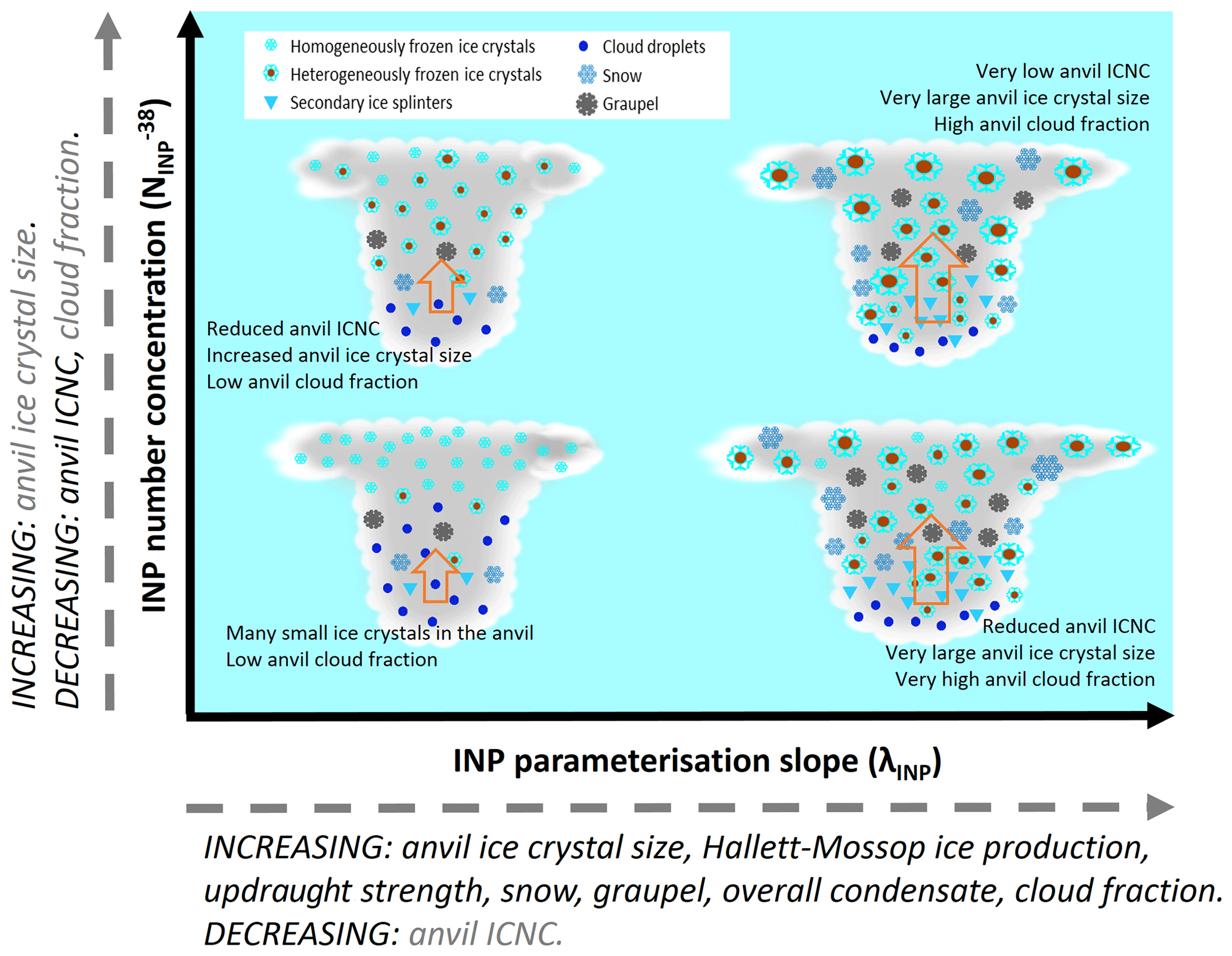
Figure 16 Schematic showing the key effects of the perturbations to absolute INP number concentration at −38 ^∘C (${N_{\text{INP}}}^{-\mathrm{38}}$) and INP parameterisation slope (λ_INP) on the deep convective cloud simulated in this study. Output variables written along the x and y axes in black indicate that they are primarily controlled by the uncertain input variable on that axis, while grey writing indicates a secondary or smaller effect of the uncertain input variable in question.

5 Discussion and conclusions

We quantify the impact of varying the limiting INP number concentration (${N_{\text{INP}}}^{-\mathrm{38}}$), the INP parameterisation slope (λ_INP), and the Hallett–Mossop splinter production efficiency (HM-eff) on the anvil properties of an idealised deep convective cloud. A schematic of the main effects identified in this study is shown in Fig. 16. Overall, we find that both λ_INP and ${N_{\text{INP}}}^{-\mathrm{38}}$ play a role in determining the anvil cloud properties, with the HM-eff being relatively unimportant in determining the anvil cloud properties. Despite this, we find that the interaction of λ_INP with HM-eff is important for determining the resultant amount of ice particle production by the Hallett–Mossop process, which in turn has large effects on the cloud development.

Anvil ICNC is strongly reduced at high-${N_{\text{INP}}}^{-\mathrm{38}}$ values, with the reduction being more pronounced at shallow-λ_INP values. Conversely, anvil ice crystal size is increased at shallow-λ_INP values, with the enhancement being more pronounced at high-${N_{\text{INP}}}^{-\mathrm{38}}$ values. This is because the lower the altitude of heterogeneous freezing, the more cloud droplets are consumed by riming and depositional growth and the lower the number of droplets that are available for either homogeneous or cold temperature heterogeneous freezing. A shallow λ_INP reduces the number of cloud droplets reaching the top of the mixed-phase regime, and a high ${N_{\text{INP}}}^{-\mathrm{38}}$ reduces the number of cloud droplets reaching the homogeneous freezing regime. Consequently, the anvil consists of a smaller number of large heterogeneously frozen crystals in a high-${N_{\text{INP}}}^{-\mathrm{38}}$ and shallow-λ_INP scenario. The ice crystals transported from the heterogeneous freezing regime to the anvil in this case are larger than those that would be frozen heterogeneously at very cold temperatures or homogeneously. Anvil cloud fraction within the time period studies is enhanced at shallow-λ_INP values, and this enhancement is lower at high-${N_{\text{INP}}}^{-\mathrm{38}}$ values. This is because a shallow λ_INP induces an invigoration effect (inferred from higher cloud updraught speeds) due to an increase in Hallett–Mossop ice production and enhanced glaciation at mixed-phase temperatures, leading to larger condensate mass divergence in the upper troposphere and a more extensive anvil. The anvil is smaller in a high-${N_{\text{INP}}}^{-\mathrm{38}}$ scenario due to the reduced ICNC and increased ice crystal size discussed above, which serves to reduce cloud lifetime.

Statistical emulation and variance-based sensitivity analysis allow us to identify complex interdependencies between input and output variables. We find that the interaction between λ_INP and ${N_{\text{INP}}}^{-\mathrm{38}}$ account for up to 30 % of the variation in values of anvil ICNC and anvil ice crystal size. The emulator surfaces help us to see variation in the importance of input parameters depending on the value of other uncertain inputs that would not otherwise be apparent in one-at-a-time tests. In particular, we identify several important interdependencies between different freezing mechanisms. For example, at high ${N_{\text{INP}}}^{-\mathrm{38}}$, λ_INP is important in determining the anvil ICNC and homogeneous freezing rates because the shallower the λ_INP, the fewer cloud droplets available to be frozen homogeneously or heterogeneously at the top of the mixed-phase regime. However, at lower ${N_{\text{INP}}}^{-\mathrm{38}}$ values, λ_INP is nearly inconsequential to homogeneous freezing rates and anvil ICNC because the ${N_{\text{INP}}}^{-\mathrm{38}}$ is low enough that a shallow λ_INP does not substantially affect the number of droplets reaching upper cloud levels. Furthermore, the dominant effect of λ_INP on many cloud properties is in part attributed to the fact that high-λ_INP values provide seed crystals for the Hallett–Mossop process, vastly increasing the number concentration of ice crystals between 5 and 7.5 km and subsequently the cloud riming and deposition rates.

The amount of Hallett–Mossop ice particle production is determined by both HM-eff and λ_INP, with a λ_INP above ∼ −0.3 ${}^{\circ }{\mathrm{C}}^{-\mathrm{1}}$ causing a jump of about an order of magnitude in Hallett–Mossop ice particle production while the effect of HM-eff is linear. A regime shift to a cloud with extensive glaciation at warm temperatures, stronger convective updraughts, larger condensate mass divergence in the upper troposphere, and a more extensive anvil occurs for λ_INP values between −0.3 and −0.1 ${}^{\circ }{\mathrm{C}}^{-\mathrm{1}}$, with the exact value of the transition depending on the ${N_{\text{INP}}}^{-\mathrm{38}}$ values (the transition occurs at steeper λ_INP values if the ${N_{\text{INP}}}^{-\mathrm{38}}$ is high). This regime change is driven by a shallow λ_INP (particularly when combined with a high ${N_{\text{INP}}}^{-\mathrm{38}}$) forming more ice crystals in the Hallett–Mossop temperature regime and thus seeding a stronger ice particle production by the Hallett–Mossop process. We find a strong enhancement in Hallett–Mossop ice particle production occurs at an INP number concentration anywhere between 10⁻⁴ to 1 L⁻¹ depending on the HM-eff. This indicates that the threshold INP number concentration needed to cause substantial SIP varies depending on the strength of the SIP mechanism in question. Whether the interaction of INP with other SIP mechanisms that operate over different temperature ranges has a similar effect on SIP production rates should be explored in the future.

Tropical cirrus can typically persist, and therefore affect radiation, in the atmosphere for days after the convective cloud that formed them has decayed (e.g. Luo and Rossow, 2004). While the simulations were not long enough to study the full life cycle of the anvil, we can infer possible implications of the uncertain input parameters on anvil lifetime based on the anvil ice crystal properties. An anvil with more numerous, smaller crystals will persist longer in the atmosphere than one with fewer, larger crystals. High-${N_{\text{INP}}}^{-\mathrm{38}}$ values lead to both fewer and larger anvil ice crystals and a slightly reduced cloud fraction, implying that deep convection generated in an environment with a high concentration of ice-nucleating aerosol, such as in high dust loading, may have a shorter lifetime than those generated in lower ${N_{\text{INP}}}^{-\mathrm{38}}$ environments. At shallow-λ_INP values, the anvil ice crystals are larger, indicating that a cloud anvil formed in the presence of an INP population with high efficiency at warmer temperatures, e.g. marine organics (Wilson et al., 2015), may have a shorter lifetime than that formed in the presence of an INP population with a steeper temperature dependence. However, this effect is compensated for by an invigoration effect (inferred from higher in-cloud vertical velocities) driven by higher rates of mixed-phase ice formation in simulations with shallow-λ_INP values, which leads to larger condensate mass divergence in the upper troposphere and a larger anvil in the timescale simulated in this study. Future studies should cover the entire life cycle of the generated anvil cirrus in order to quantify the resultant lifetime of the convective anvil due to compensation between these two effects of λ_INP and ${N_{\text{INP}}}^{-\mathrm{38}}$.

We demonstrate with the present study that statistical emulation is a powerful tool for visualising and quantifying the relationships between cloud responses and different uncertain parameters (Fig. 8). However, statistical emulation struggles to accurately represent cloud responses where there is a significant regime shift at shallow λ_INP (Figs. 10 and 14), for example, the anvil cloud fraction. We therefore suggest that emulation be used alongside traditional analysis methods for the further study of the complex processes occurring within deep convective clouds, particularly where sudden transitions or regime shifts are evident or likely. The use of Latin hypercube sampling to capture cloud responses over the full realistic parameter space to multiple uncertain input parameters is very effective, even without undertaking statistical emulation of the simulation data.

The microphysical effects of the variations in INP number concentrations and INP parameterisation slope detailed here build on the results of Hawker et al. (2021) and further our understanding of the role of these two uncertain inputs on deep convection. In both the complex cloud-field simulation of Hawker et al. (2021) and the idealised deep convective cloud presented here, INPs in the warm mixed-phase region enhance Hallett–Mossop ice particle production and increase snow and graupel formation, leading to an invigoration effect, more cloud condensate, and an increased cloud fraction at mixed-phase cloud levels. INPs in the mixed-phase region also reduce homogeneous ice production, leading to reduced overall column-integrated ICNCs in both studies. Conversely, in the Hawker et al. (2021) study, shallow-λ_INP values led to a reduced cloud fraction above 9 km due to reduced ice particle production by homogeneous freezing. In the deep convective cloud simulated here, a shallow λ_INP leads to an increased anvil cloud fraction due to an invigoration effect caused by enhanced ice formation and latent heat release in the mixed-phase cloud region. This indicates that the microphysical effects of INPs and the interaction of INPs with the Hallett–Mossop process are relatively consistent between realistic and idealised case studies. However, the consequences of microphysical changes due to INPs on the cloud macro-physical properties such as cloud fraction and outgoing radiation can be different depending on the specific conditions of the simulation and the type of cloud being perturbed. For example, the deep convective cloud simulated here was initiated with a relatively strong warm bubble perhaps predisposing the cloud fraction to be more sensitive to enhancements in an already strong convective updraught strength than the more realistic clouds in the Hawker et al. (2021) study. This study has enhanced our understanding of aspects of cloud microphysical behaviours that was not fully explained in Hawker et al. (2021). For example, in both studies a reduction in homogeneous freezing rates occurs where there are high INP number concentrations at low temperatures, and the results from this study indicate that it is a high ${N_{\text{INP}}}^{-\mathrm{38}}$ rather than a steep λ_INP that is the main driver of this effect, a distinction that we were unable to make in the previous study. The differences in resolution between the two studies (250 m (here) and 1 km; Hawker et al., 2021) may also cause divergences in the microphysical responses of clouds to perturbations (Varble et al., 2020).

This work highlights the complexity of interactions between mixed-phase ice processes and the challenge of representing them accurately in numerical weather prediction models. Our work indicates that the sensitivity of deep convective cloud properties to mixed-phase ice processes varies depending on ambient ice-nucleating aerosol concentrations (e.g. absolute dust concentrations) as well as the efficiency of the available ice-nucleating aerosol (e.g. whether the INP number concentration consists of dust or marine organic particles). The potential for ice particle production by INPs and SIP to impact anvil cirrus ice properties also presents a challenge for climate models. Climate models do not typically use INP number concentrations to determine ice water path and the resultant outgoing radiation, and this is an important area for future work (Baran et al., 2014; Waliser et al., 2009). The role of the temperature dependence of INP number concentration in determining the observed cloud properties indicates the importance of quantifying the concentration of INP at all mixed-phase temperatures, adding to work by, for example, Hawker et al. (2021), Liu et al. (2018), Shi and Liu (2019), and Takeishi and Storelvmo (2018). Furthermore, the temperature dependence of the INP parameterisation had a substantial effect on Hallett–Mossop ice particle production rates, indicating that heterogeneous freezing can be an important determinant of deep convective cloud properties by affecting SIP mechanisms, even when heterogeneous freezing is not the dominant mechanism of ice formation in the SIP region.

Appendix A

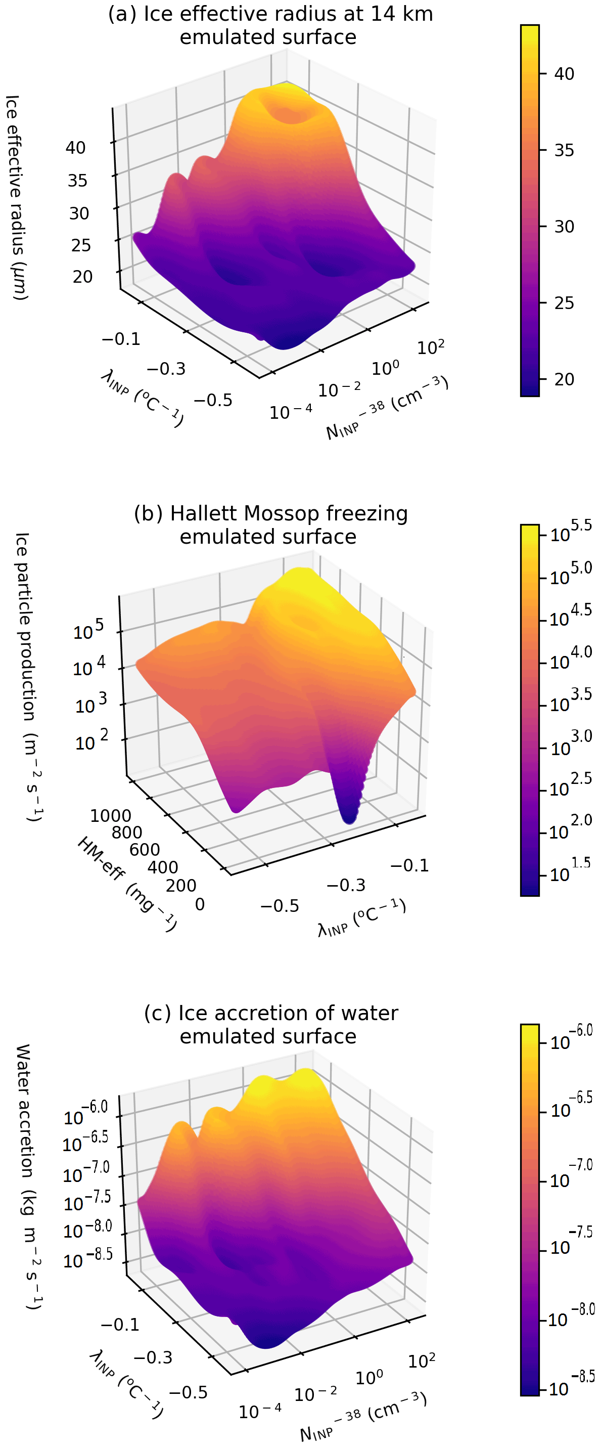
Figure A1 Emulator response surfaces. Prediction of ice effective radius (a), Hallett–Mossop ice particle production (b), and accretion of water by ice (c) by the emulator. Shown in panels (a) and (c) are the emulated response surfaces at a fixed HM-eff of 350 splinters produced per milligram of rimed liquid. Shown in panel (b) is the emulated response surface at a fixed ${N_{\text{INP}}}^{-\mathrm{38}}$ of 1 cm⁻³. The colours indicate output values and are the same range and units as the z axis. Panel (a) is the average of the cloud property between 150 and 240 min (anvil stage) of the simulation, while panels (b) and (c) are the average of the relevant cloud property between 60 and 180 min (convective stage) of the simulation.

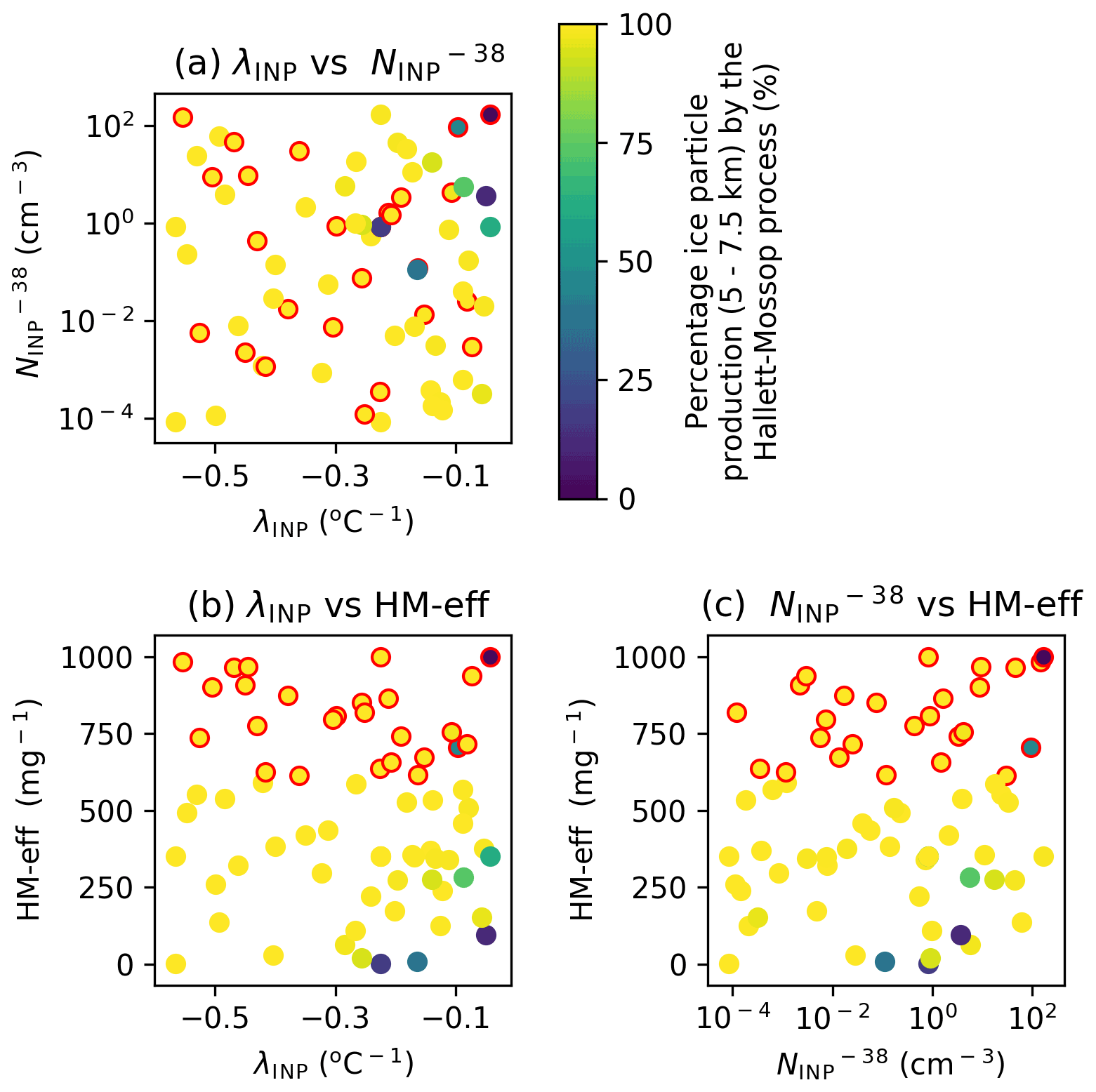
Figure A2 Source of ice crystals in the Hallett–Mossop region of the simulated deep convective cloud. Percentage of ice crystals produced between 5 and 7.5 km altitude that are produced from the Hallett–Mossop process [i.e. (Hallett–Mossop ice crystals/Hallett–Mossop and INP-produced ice crystals) × 100]. Simulations with a HM-eff above 600 splinters mg⁻¹ are indicated with a red outline. Ice particle production rates are calculated from the convective stage of the simulation (between 60 and 180 min).