the Creative Commons Attribution 4.0 License.
the Creative Commons Attribution 4.0 License.
 | 25 Nov 2021
Changes in PM2.5 concentrations and their sources in the US from 1990 to 2010
Ksakousti Skyllakou
Pablo Garcia Rivera
Brian Dinkelacker
Eleni Karnezi
Ioannis Kioutsioukis
Carlos Hernandez
Peter J. Adams
Spyros N. Pandis
Significant reductions in emissions of SO2, NOx, volatile organic compounds (VOCs), and primary particulate matter (PM) took place in the US from 1990 to 2010. We evaluate here our understanding of the links between these emissions changes and corresponding changes in concentrations and health outcomes using a chemical transport model, the Particulate Matter Comprehensive Air Quality Model with Extensions (PMCAMx), for 1990, 2001, and 2010. The use of the Particle Source Apportionment Algorithm (PSAT) allows us to link the concentration reductions to the sources of the corresponding primary and secondary PM. The reductions in SO2 emissions (64 %, mainly from electric-generating units) during these 20 years have dominated the reductions in PM2.5, leading to a 45 % reduction in sulfate levels. The predicted sulfate reductions are in excellent agreement with the available measurements. Also, the reductions in elemental carbon (EC) emissions (mainly from transportation) have led to a 30 % reduction in EC concentrations. The most important source of organic aerosol (OA) through the years according to PMCAMx is biomass burning, followed by biogenic secondary organic aerosol (SOA). OA from on-road transport has been reduced by more than a factor of 3. On the other hand, changes in biomass burning OA and biogenic SOA have been modest. In 1990, about half of the US population was exposed to annual average PM2.5 concentrations above 20 µg m−3, but by 2010 this fraction had dropped to practically zero. The predicted changes in concentrations are evaluated against the observed changes for 1990, 2001, and 2010 in order to understand whether the model represents reasonably well the corresponding processes caused by the changes in emissions.
- Article
(15396 KB) - Full-text XML
-
Supplement
(850 KB) - BibTeX
- EndNote


During recent decades, regulations by the US Environmental Protection Agency (EPA) have led to significant reductions in the emissions of SO2, NOx, VOCs, and primary PM from electrical utilities, industry, transportation, and other sources (US EPA, 2011). Xing et al. (2013) estimated that, from 1990 to 2010, emissions of SO2 in the US were reduced by 67 %, NOx by 48 %, non-methane VOCs by 49 %, and primary PM2.5 by 34 %. An increase in ammonia emissions by 11 % was estimated for this 20-year period. At the same time, there have been significant observed reductions in the ambient PM2.5 levels in practically all areas of the US (Meng et al., 2019). However, our ability to link these changes in estimated emissions to the observed changes in PM2.5 faces challenges. The available PM2.5 composition and mass concentration measurements are sparse in space and are quite limited before 2001. Three-dimensional chemical transport models (CTMs) are well suited to help address this problem, since they simulate all the major processes that impact PM2.5 concentrations and transport.
There have been several efforts to quantify historical changes in PM2.5 levels and composition. These rely heavily on measurements (both ground and satellite for the more recent changes) and on a number of statistical techniques including land-use regression models to calculate the concentrations of PM2.5 over specific areas and periods (Eeftens et al., 2012; Beckerman et al., 2013; Ma et al., 2016; Li et al., 2017a). Milando et al. (2016) used positive matrix factorization (PMF) of PM measurements to interpret the observed trends of PM2.5 from 2004 to 2011 in Detroit and Chicago. They concluded that as secondary sulfate was declining, emissions from biomass burning, vehicles, and metal sources are becoming relatively more important. More recent efforts also include applications of chemical transport models. For example, Meng et al. (2019) estimated historical PM2.5 concentrations over North America from 1981 to 2016, combining the predictions of GEOS-Chem, satellite remote sensing, and ground-based measurements. That study focused on the estimation of total PM2.5 levels to assess long-term changes in exposure and associated health risks. The composition of PM2.5 and its sources were not analyzed in that work. Jin et al. (2019) combined information from ground-based observations, remote sensing, and chemical transport models to estimate that the PM2.5-related mortality decreased by 67 % in New York State from 2002 to 2012. Li et al. (2017b) combined in situ and satellite observations with the global CTM, GEOS-Chem, to quantify global and regional trends in the chemical composition of PM2.5 over 1989–2013. They concluded that the predicted average trends for North America were consistent with the available measurements for PM2.5, secondary inorganic aerosols, organic aerosols, and black carbon. Nopmongcol et al. (2017) used CAMx with the Ozone Source Apportionment Technology (OSAT) and Particulate Source Apportionment Technology (PSAT) algorithms for 6 different years within 5 decades (1970–2020) to calculate the contributions from different emission sources to PM2.5 and O3 in the US. The same meteorology and the same natural emissions (including wildfires) were used for all 6 simulated years. The authors concluded that the contribution of electrical generation units (EGUs) and on-road sources to fine PM has declined in most areas, while the contributions of sources such as residential, commercial, and fugitive dust emissions stand out as making large contributions to PM2.5 that are not declining. The use of constant meteorology did not allow the direct evaluation of these predictions.
In this study, we use period-specific meteorological data and source-resolved emissions for every year simulated to estimate the concentrations, composition, and sources of PM2.5 over 20 years in the US. Three specific years are used as snapshots of US air quality in time. Given that significant emissions changes have taken place over the decades between the examined years, the predicted concentration changes reflect mostly changes in these emissions plus some year-to-year meteorological variability. The model predictions are compared with the available measurements. The sources responsible for the PM2.5 reductions in various areas of the country are identified, and their contribution to the reductions is quantified. We also quantify trends in population exposure and estimated health outcomes.
2.1 Particulate Matter Comprehensive Air Quality Model with Extensions (PMCAMx)
PMCAMx (Karydis et al., 2010; Murphy and Pandis, 2010; Tsimpidi et al., 2010; Posner et al., 2019) uses the framework of the CAMx model (Environ, 2006) to describe horizontal and vertical advection and diffusion, wet and dry deposition, and gas- and aqueous-phase chemistry. A 10-size section (30 nm to 40 µm) aerosol sectional approach is used to dynamically track the evolution of the aerosol mass distribution. The aerosol species modeled include sulfate, nitrate, ammonium, sodium, chloride, elemental carbon, mineral dust, and primary and secondary organics. The Carbon Bond 05 (CB5) mechanism (Yarwood et al., 2005) is used in this application of PMCAMx for gas-phase chemistry calculations. The version of CB5 used here includes 190 reactions of 79 surrogate gas-phase species. For condensation and evaporation of inorganic species, a bulk equilibrium approach was used, assuming equilibrium between the bulk inorganic aerosol and gas phases. The partitioning of each semi-volatile inorganic species between the gas and aerosol phases is determined by the ISORROPIA aerosol thermodynamics model (Nenes et al., 1998). The mass transferred between the two phases in each step is distributed to the size sections using weighting factors based on the effective surface area of each size bin (Pandis et al., 1993). Organic aerosols (primary and secondary) are simulated using the volatility basis set approach (Donahue et al., 2006). For primary organic aerosols (POA), eight volatility bins, ranging from 10−1 to 106 µg m−3 at 298 K saturation concentration, are used. Secondary organic aerosols (SOA) are split between aerosol formed from anthropogenic sources (aSOA) and from biogenic ones (bSOA) and modeled with four volatility bins (1, 10, 102, 103 µg m−3) (Murphy and Pandis, 2009). NOx-dependent yields (Lane et al., 2008) are used. For better representation of the chemistry in NOx plumes, the plume-in-grid modeling approach of Karamchandani et al. (2011) has been used for the major point sources following Zakoura and Pandis (2019).
2.2 PSAT
PSAT (Wagstrom et al., 2008; Wagstrom and Pandis, 2011a, b; Skyllakou et al., 2014, 2017) is an efficient algorithm that tracks and computes the contributions of different sources to pollutant concentrations. The advantages of PSAT are that it runs in parallel with PMCAMx, so there is no need to modify the CTM for different applications, and that it is quite computationally efficient. PSAT takes advantage of the fact that the molecules of each pollutant at each location, regardless of their source, have the same probability of reacting, depositing, or getting transported to avoid repeating the simulations of these processes. For secondary species, it follows the apportionment of their precursor vapors. For example, the apportionment of secondary organic aerosol is based on the apportionment of VOCs or IVOCs, sulfate on SO2, nitrate on NOx, and ammonium on NH3.
In this study, we use the version of PSAT developed by Skyllakou et al. (2017) that is compatible with the volatility basis set to calculate the contribution of each emission source to the concentration of PM2.5 and its components.
PMCAMx-PSAT was applied over the continental United States (CONUS) for the years 1990, 2001, and 2010 using a grid of 132 by 82 cells with horizontal dimensions of 36 km by 36 km (covering an area of 4752×2952 km) and 14 layers of varying thickness up to an altitude of approximately 13 km. We selected this resolution as it has been shown to be a viable option for keeping computational and storage demands manageable while providing sufficient quality for long-term simulations and air quality planning applications (Gan et al., 2016). This coarse resolution introduces errors in areas where there are significant PM2.5 gradients in space, including California and urban areas in the rest of the western US.
3.1 Meteorology
Meteorological simulations were performed with the Weather Research Forecasting model (WRF v3.6.1) over the CONUS area, with a horizontal resolution of 12×12 km and 36 vertical (sigma) levels up to a height of about 20 km. The simulations were executed using 3 d re-initialization from observations. Initial and boundary conditions were generated from the ERA-Interim global climate re-analysis database, together with the terrestrial data sets for terrain height, land use, soil categories, etc., from the United States Geological Survey database. The WRF modeling system was prepared and configured in a similar way to that described by Gilliam and Pleim (2010). For the model physical parameterization, the Pleim–Xiu land surface model (Xiu and Pleim, 2002) was selected. Other important WRF physics options used in this study include the Rapid Radiative Transfer Model/Dudhia radiation schemes (Iacono et al., 2008), the Asymmetric Convective Model version 2 for the planetary boundary layer (Pleim, 2007a, b), the Morrison double-moment cloud microphysics scheme (Morrison et al., 2008), and version 2 of the Kain–Fritsch cumulus parameterization (Kain, 2004). The selected WRF configuration is recommended for air quality simulations (Hogrefe et al., 2015; Rogers et al., 2013).
3.2 Emissions
Emissions for the simulations were obtained from the internally consistent, historical emission inventories of Xing et al. (2013) that include source-resolved gas and primary particle emissions. Point source sectors include EGUs included in the EPA's Integrated Planning Model (IPM), industrial sources not included in the IPM (non-EGU), and all other point sources in Canada and Mexico. Area sources include on-road emissions in the US, Canada, and Mexico, off-road emissions for the entire domain, and all remaining non-biogenic sources. We used our WRF meteorology to drive the Model of Emissions of Gases and Aerosols from Nature (MEGAN3) (Jiang et al., 2018) using the default emission factors for all years to generate biogenic emissions for the CONUS domain.
In this application of PSAT, we used six different emission categories based on those described above plus initial and boundary conditions which are each tracked separately by the model as different “sources”. As a result, the emission source categories used are “road”, which includes road emissions over the US, “non-road”, which includes the off-road emissions of the entire domain, “EGU”, “non-EGU” as described above, “other”, which includes the sum of the other point and area sources plus the “on-road” emissions from Canada and Mexico, and finally biogenic emissions. Figure 1 depicts the total annual emissions for each source and each year.
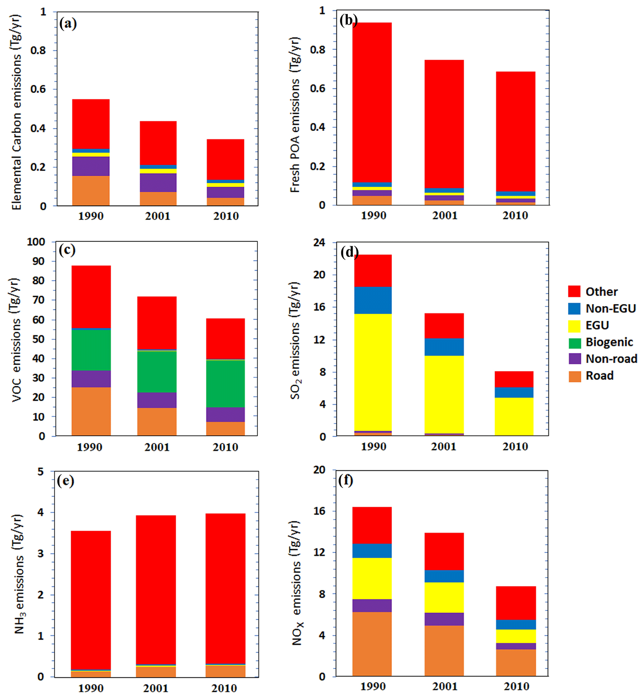
Figure 1Annual emissions by each source for the whole domain for (a) elemental carbon, (b) fresh POA, (c) non-methane VOCs, (d) SO2, (e) NH3, and (f) NOx.
Biomass burning (included in the “other” category) was the dominant source of EC and remained relatively constant during the simulated period. The second most important source of EC was road transport, with the corresponding emissions having been reduced by a factor of 3.5 from 1990 to 2010. The overall reduction in EC emissions was 40 %.
Biomass burning and other sources were the dominant source also of POA, with almost constant contributions. Based on the emissions that Xing et al. (2013) reported in the category “other”, we can estimate that biomass burning was responsible for 46 % of the total “other” POA emissions. This contribution increased to 80 % in 2001 and 83 % in 2010. The PM emitted from biomass burning, according to the inventory, is similar for these 3 years (Xing et al., 2013). The second most important source of POA during 1990 was road transport, contributing 5 %. This emission source was reduced by a factor of 3.5 from 1990 to 2010. Overall POA emissions in the inventory were reduced by 27 % from 1990 to 2010.
Emissions of VOCs by on-road sources were reduced by a factor of 3.5 during these 20 years. On the other hand, the VOCs emitted by non-road transport decreased by only 8 %. The biogenic VOC emissions varied from year to year based on the prevailing meteorology, but their changes were less than 20 %. The total (anthropogenic and biogenic) VOC emissions decreased by 31 % from 1990 to 2010.
The emissions of the most important SO2 source, EGUs, were reduced by 33 % from 1990 to 2001 and by 67 % from 1990 to 2010. This resulted in a 64 % reduction in the total SO2 emissions over these 20 years.
For NH3, the most important source is agriculture (included in the “other” category), and the corresponding emissions increased by 9 % during these 20 years.
Road transportation is one of the major NOx sources, with the corresponding emissions having been reduced by 21 % from 1990 to 2001 and by 58 % from 1990 to 2010. The second most important source of NOx in 1990 was the EGUs, which emitted 25 % less NOx in 2001 and 66 % less NOx in 2010 compared to 1990. Total NOx emissions in the inventory were 47 % lower in 2010 compared to 1990.
4.1 Annual average concentrations and sources
We examine first the source apportionment results of PMCAMx-PSAT for the major components of PM2.5 for the 3 simulated years.
On-road transportation was a major source of EC, especially in urban areas in 1990 (Fig. 2). The EC concentrations originating from this source were reduced by more than a factor of 3 from 1990 to 2010. The industrial sources (EGU and non-EGU) contributed less than 0.1 µg m−3 of EC in all areas during these years. The “other” source, which includes all types of biomass burning, was the most important source during the simulated period. Long-range transport (LRT), which represents the transport from areas outside of the domain, contributed approximately 0.1 µg m−3.
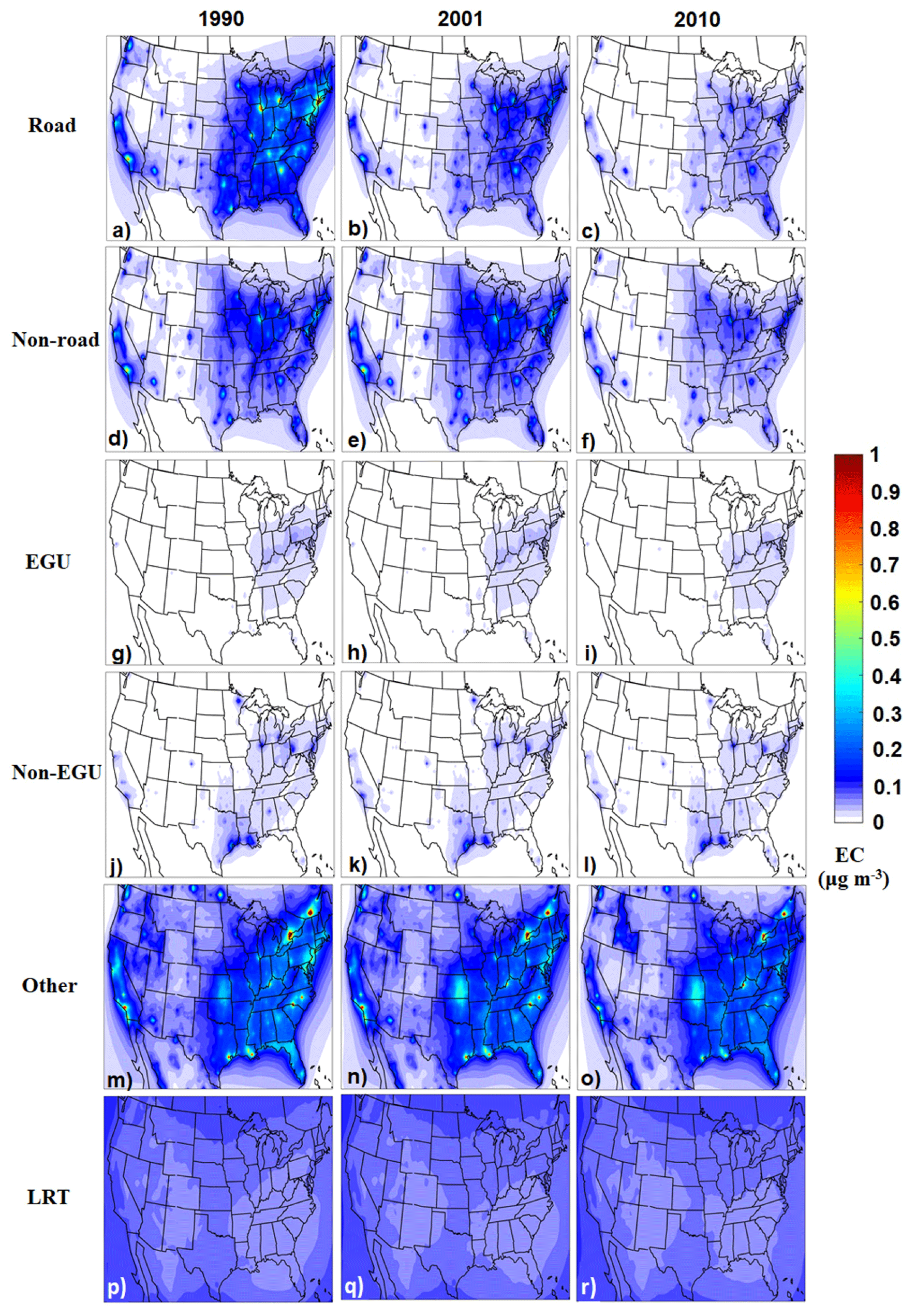
Figure 2Predicted annual average ground-level PM2.5 elemental carbon concentrations per source for 1990, 2001, and 2010.
The predicted average total OA levels defined as the sum of POA and SOA are shown in Fig. 3. The OA originating from road transport was about 0.7 µg m−3 during 1990 over the eastern US, but it was reduced to less than 0.5 µg m−3 during 2010. “Non-road” transport and “non-EGU” emission sources had smaller contributions to OA, with less than 0.2 µg m−3 in most areas during all years. Biogenic SOA was almost 1 µg m−3 over the southeastern US during both 1990 and 2001, but during 2010 it had higher concentrations in some areas. Especially in the south due to local meteorology, predicted SOA was much higher compared to 1990. In 2010, the biogenic VOC concentrations were on average 15 % higher compared to 1990, due mainly to the meteorological conditions during these 2 specific years. This small increase is consistent with the biogenic VOC emissions estimated by Sindelarova et al. (2014). Also, high OA concentrations were predicted to originate from biomass burning during 1990. The average contribution of long-range transport OA was approximately 0.6 µg m−3.
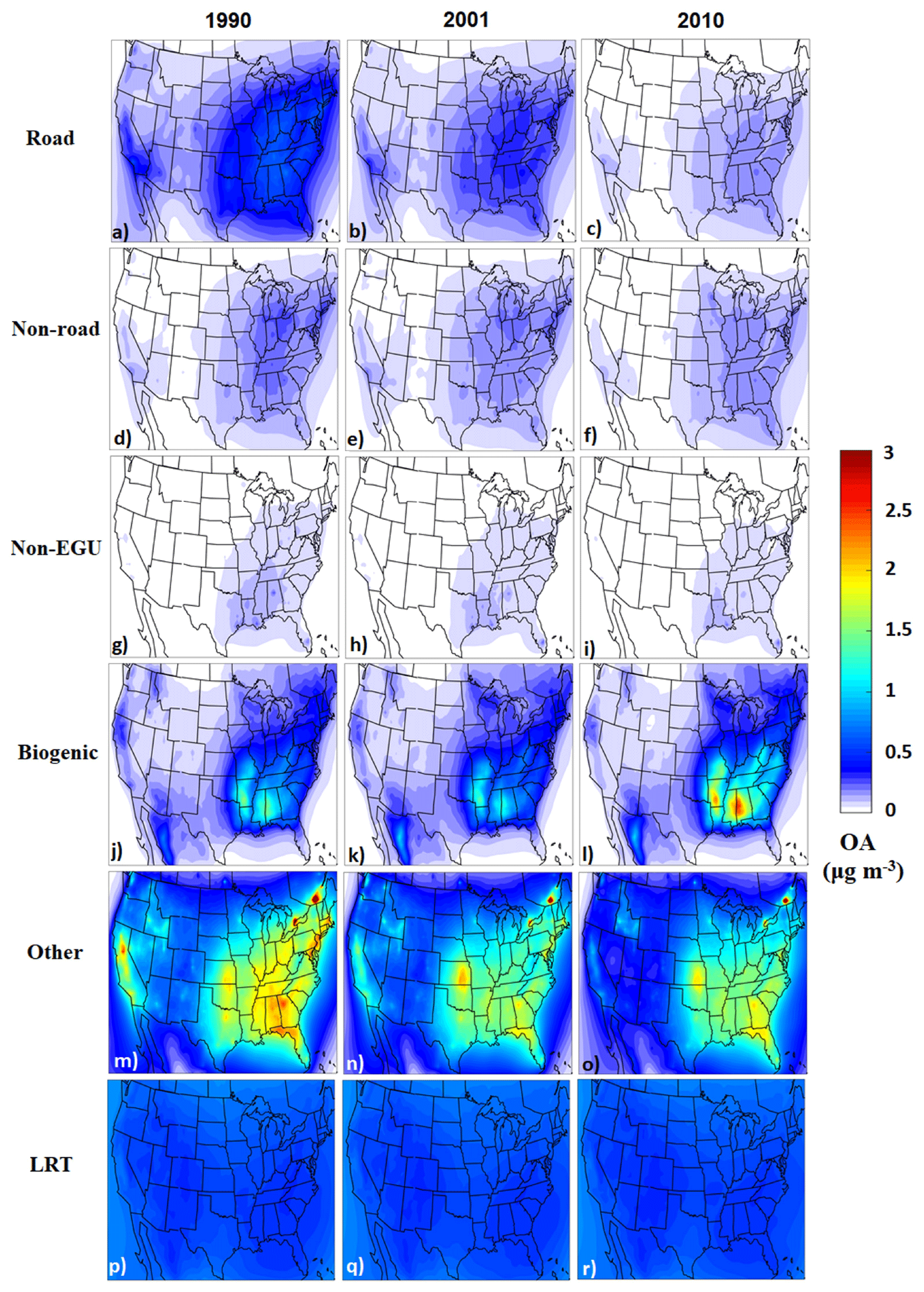
Figure 3Predicted annual average ground-level PM2.5 organic (primary plus secondary) aerosol concentrations per source for 1990, 2001, and 2010. The EGU contributions are low and are not shown.
Sulfate was the dominant component of PM2.5 in the eastern US in 1990, and the EGUs were its dominant source, contributing more than 5 µg m−3 over wide areas of the east (Fig. 4). The corresponding sulfate concentrations from EGUs were reduced to 3 µg m−3 in 2001 and to 1.5 µg m−3 in 2010 due to the dramatic reduction in these SO2 emissions over these 20 years. Sulfate concentrations originating from non-EGU and other emission sources were 1 µg m−3 or less during all years. Long-range transport contributed approximately 0.9 µg m−3 to the sulfate levels during the simulated period.
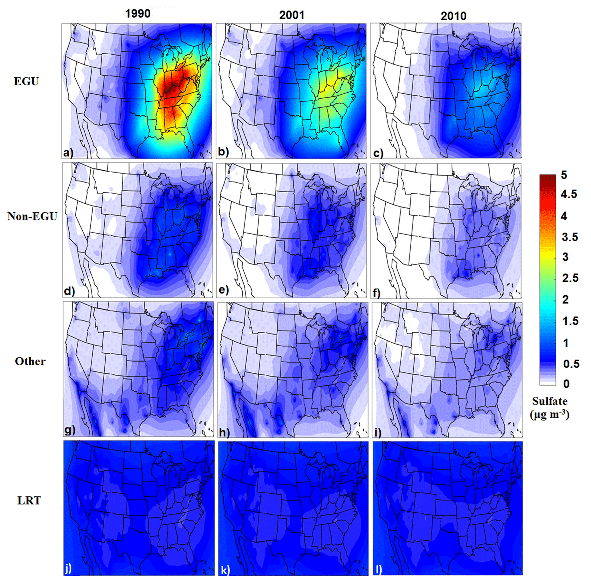
Figure 4Predicted annual average ground-level PM2.5 sulfate concentrations per source for 1990, 2001, and 2010. The on-road, non-road, and biogenic contributions are low and are not shown.
4.2 Evaluation of the model predictions
The model was evaluated on both an annual and daily basis against ground-level measurements from the IMPROVE and CSN networks (STN US EPA, 2002; IMPROVE, 1995). The metrics used in the main analysis include the normalized mean bias (NMB), the normalized mean error (NME), the mean bias (MB), the mean absolute gross error (MAGE), the fractional bias (FBIAS), and the fractional error (FERROR) (Fountoukis et al., 2011):
where Pi represents the model-predicted value for site i, Oi is the corresponding observed value, and n is the total number of sites. During 1990, there were only 27 measurement sites for PM2.5 composition, all part of the IMPROVE network, but this number increased dramatically in 2001 to more than 100 and in 2010 to approximately 300 stations. There was almost an order of magnitude more measurements and stations for just PM2.5 mass concentration. The results for annual evaluation are summarized in Table 1 and for the evaluation based on daily average concentrations in Table 2.
Table 1Evaluation metrics for annual average concentrations of PM2.5 and for its major components for each examined year.
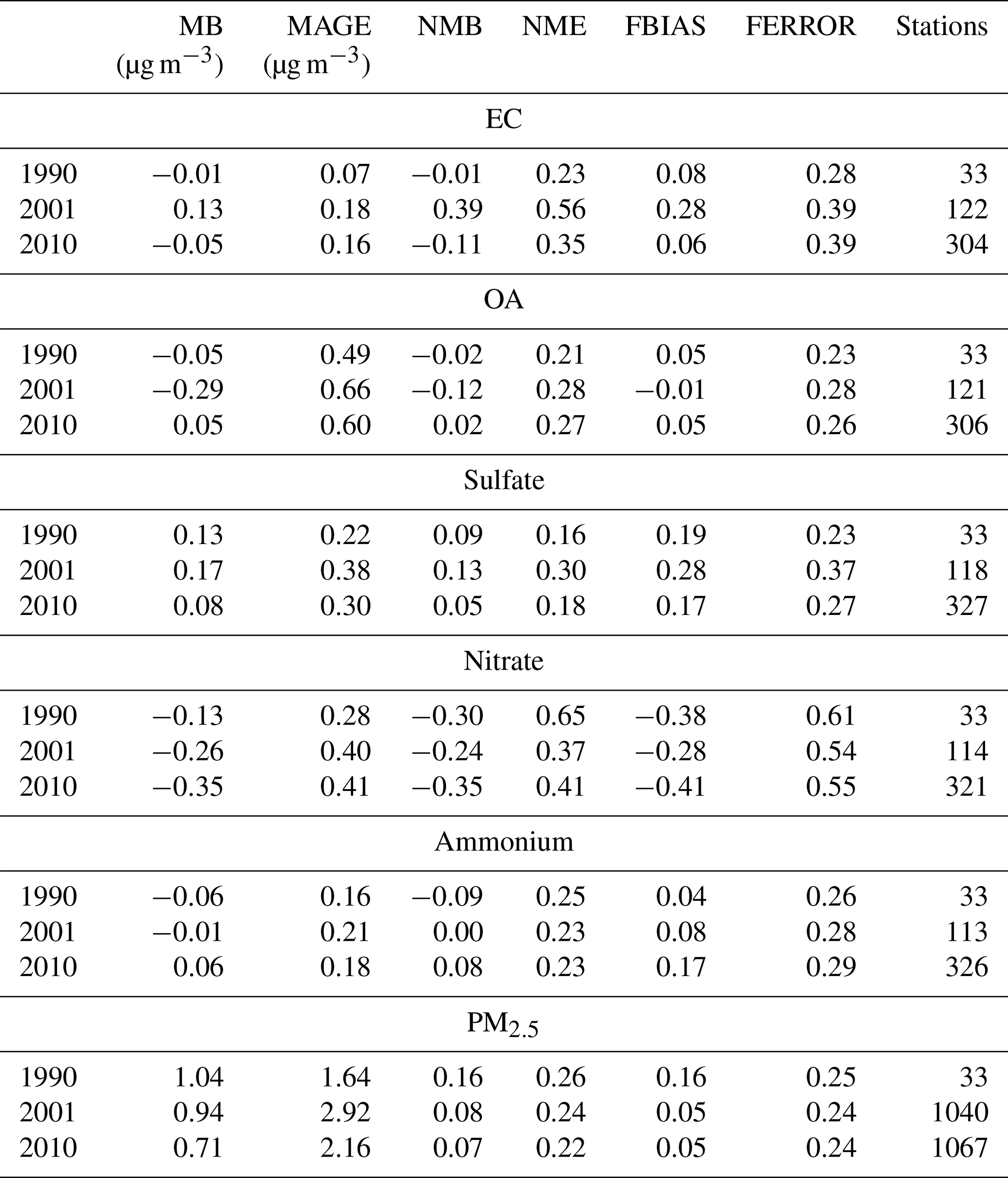
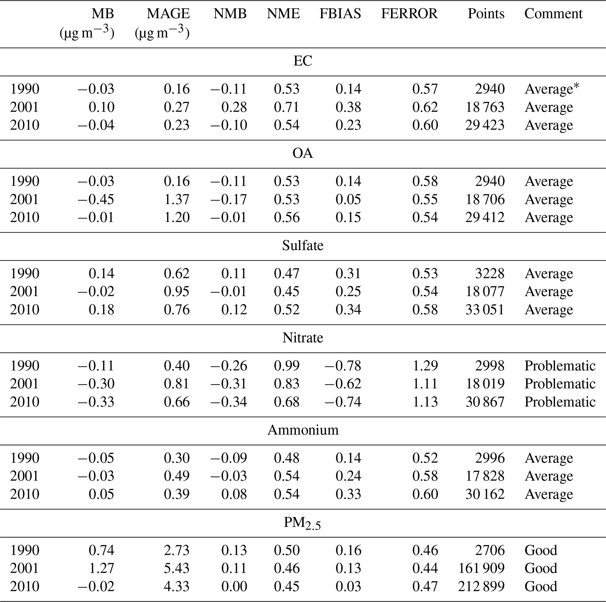
Table 2Evaluation metrics for daily average concentrations of PM2.5 and for its major components for each examined year.
* Following Morris et al. (2005) criteria. Good: FBIAS ≤ ± 0.30, FERROR ≤ 0.50. Average: FBIAS ≤ ±0.60, FERROR ≤ 0.75. Problematic: FBIAS > ±0.60, FERROR > 0.75.
PMCAMx reproduced the annual average PM2.5 concentrations with an absolute fractional bias of less than 16 % and a fractional error of less than 25 % (Table 1). The highest bias was found for 1990, when measurements from only 33 sites were available. During 2001 and 2010 when more than 1000 stations were operational, the PM2.5 fractional bias was only 5 %. The model tends to underpredict PM2.5 in the sites in the west and especially in California and tends to overpredict in the rest of the country (Table S1 in the Supplement). The OA annual average concentrations were also reproduced with little bias (less than 5 %) and fractional error less than 30 %. The model had a slight tendency towards overprediction of sulfate with a fractional bias of 17 %–28 % depending on the year, but the fractional error was still modest at 23 %–37 %. The EC annual levels were reproduced with little bias (FBIAS equal to 6 %–8%) during 1990 and 2010, but there was a tendency towards overprediction during 2001 (FBIAS = 28 %), while the fractional error was modest (28 %–39 %). The nitrate levels, especially in the high-nitrate areas, were underpredicted (FBIAS ranged from −28 % to −41%), and the error was relatively high compared to all other components (54 %–61 %). Finally, the model did a relatively good job reproducing the ammonium levels (FBIAS 4 %–17 % and FERROR 26 %–29 %). The low grid resolution of these simulations introduced significant errors in California, where significant spatial gradients are encountered. The evaluation results without the Californian sites are summarized in Table S2. For example, the nitrate bias is −19 % to −34 % when the measurements in California are excluded from the evaluation.
According to Morris et al. (2005), the level of the performance of the model for daily resolution is considered excellent if it meets the following criteria: FBIAS ≤ ±0.15 and FERROR ≤ 0.35. It is good if FBIAS and FERROR ≤ 0.50, it is average if FBIAS ≤ ±0.60 and FERROR ≤ 0.75, and it is problematic if FBIAS > ±0.60 and FERROR > 0.75. Based on these criteria, the ability of the model to reproduce the daily average concentrations during all simulated years is good for PM2.5, average for EC, OA, sulfate, and ammonium, and problematic for nitrate. The daily PM2.5 concentrations, for which there are many more stations and measurements in 2001 and 2010, are reproduced with a fractional bias of 3 % to 13 % and a fractional error of less than 50 % (Table 2). For 1990, there is little bias, while there is a small tendency towards overprediction in the later years.
The version of PMCAMx used in these simulations has difficulties reproducing the nitrate levels. There several reasons for these problems, including the spatial resolution used here and the assumption of bulk equilibrium, which will be analyzed further in future work. PMCAMx has a small tendency towards underprediction of the OA and the EC. There is also a tendency towards overprediction of the sulfate and, as a result, the ammonium too.
We also followed the approach suggested by Emery et al. (2017) for the characterization of the model performance. This approach relies on the NMB, NME, and correlation coefficient (r) as metrics. The results of the corresponding analysis are summarized in Tables S4, S5, and S6 and suggest that the model is acceptable for all components and periods, with two exceptions: sulfate during 2010 and ammonium during 2001.
One of the important results of this evaluation is the relatively consistent performance of PMCAMx during the different years. The use of a consistent emission inventory, consistent meteorology, and measurements has probably contributed to this outcome.
4.3 Regional contributions of sources to PM2.5 components
The US was divided into seven regions (Fig. 5) to facilitate the spatial analysis of the source contributions and their changes during the simulated period. The Northeast (NE) region includes major cities such as New York, Boston, Philadelphia, Baltimore, and Pittsburgh, while the Mideast (ME) includes the Ohio River valley area with a number of electrical generation units. The Midwest (MW) has significant agricultural activities, while much of the West (WE) is relatively sparsely populated. California (CA) was kept separate from the other western regions. The southern US was split into a Southeast region (SE) with significant biogenic emissions and the Southwest (SW) with much less vegetation.
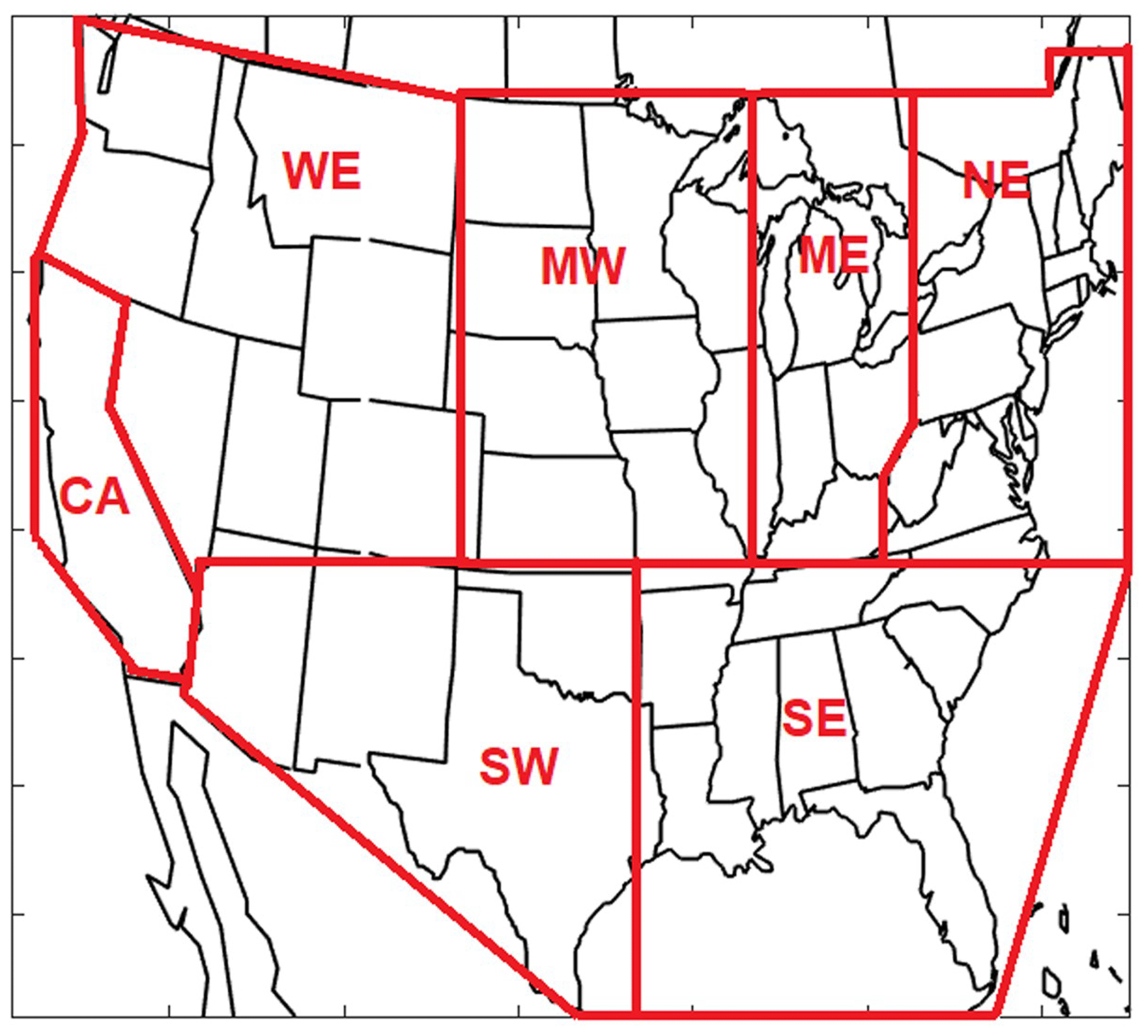
Figure 5Definition of the seven regions used in the analysis.
Figure 6a shows the predicted average concentrations of EC for each year in each region. The highest concentrations for 1990 were predicted in the Mideast, followed by the Northeast and California. Biomass burning, included in the “other” source, was the dominant source of EC in all regions, with relatively constant concentrations through the years, except from CA, where the contribution from this source in 1990 was much higher due to the annual variation in fires. There was significant reduction in the EC levels in all regions except for the West, where the EC originates mainly from biomass burning and long-range transport. The highest reductions were predicted for the eastern US. Figure 6b shows the population exposure (Walker et al., 1999), which is calculated in this work as the product of the average annual concentration of each computational cell times the population living in the cell. The US population distribution was calculated for each year based on the US Census Bureau (2019) data and is different for 1990, 2001, and 2010. The population distribution of 2001 is assumed to be the same as that of 2000. The population exposure is significant in areas with high population density, for example in CA. The US population increased from 1990 to 2010 by almost 24 %. This increase would have led to a corresponding increase in total population exposure if the emissions had not changed during this period.
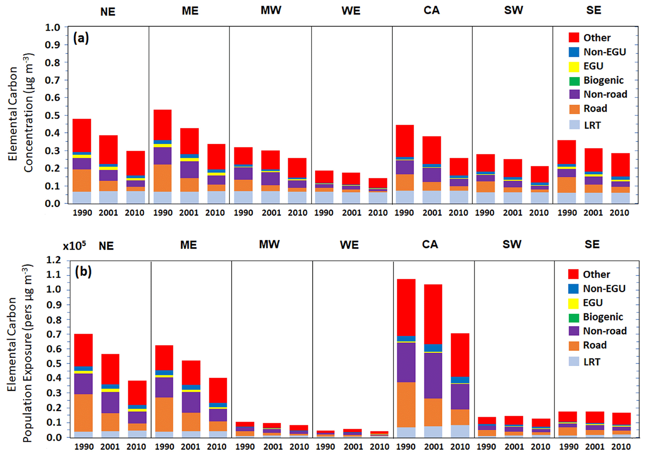
Figure 6Sources of PM2.5 EC for the different regions during 1990, 2001, and 2010 for (a) average concentrations (µg m−3) and (b) population exposure (persons µg m−3).
The source contributions to the annual average concentrations of OA are depicted in Fig. 7a. The predicted concentrations of OA in 1990 in the eastern US (NE, SE, and ME regions) were almost 3 µg m−3 and, in the other regions, less than 2.5 µg m−3. OA originating from biomass burning dominated the concentrations of OA during all years and regions. Biogenic SOA was the second most significant OA component in the Southeast. OA originating from on-road transport contributed, according to the model, almost 0.5 µg m−3 during 1990 and almost 0.2 µg m−3 during 2010 in the eastern US. Significant reductions in OA are predicted for the Northeast, Mideast, and California but moderate reductions for the Midwest, West, and Southwest. The OA in the Southeast has more complex behavior due to the predicted increase in biogenic SOA in 2010 that leads to a small increase in the total OA compared to 2001. The population exposure for OA (Fig. 7b) is almost the same for the Northeast and Mideast during 1990, and it decreased during 2001 and 2010. For the Midwest, West, and Southwest, the population exposure to OA remained almost constant through the years. For all regions, the highest population exposure was due to biomass burning and the “other” sources. In addition, 20 % of the population exposure was due to road transport during 1990 in the highest populated areas (NE, ME, and CA), but this percentage was reduced to almost 10 % during 2010.
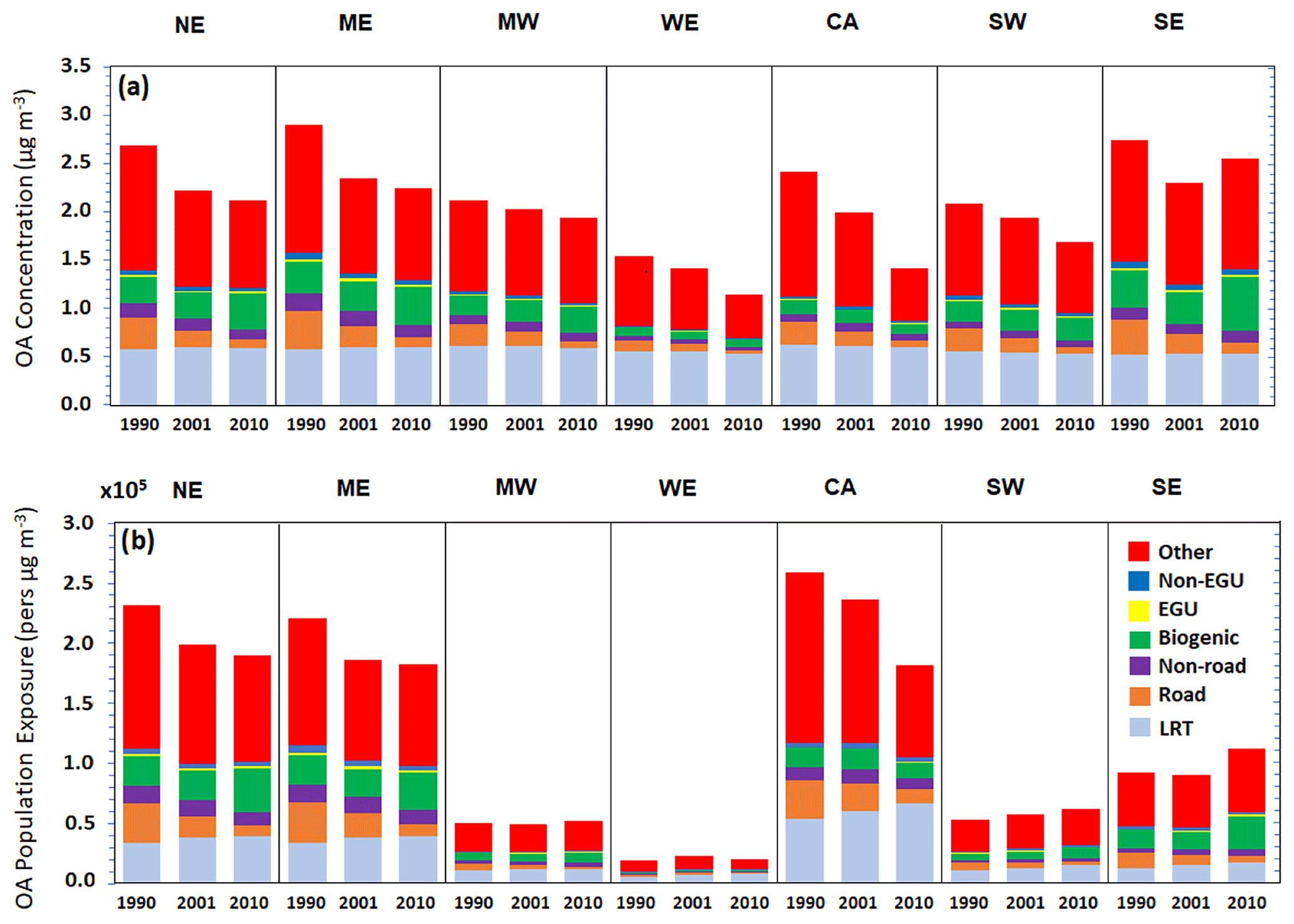
Figure 7Sources of PM2.5 OA for the different regions during 1990, 2001, and 2010 for (a) average concentrations (µg m−3) and (b) population exposure (persons µg m−3).
The highest concentrations of sulfate for 1990 are predicted in the eastern US (NE, ME, and SE) in regions downwind of the EGUs, which are the dominant SO2 source in these areas (Fig. 8a). The drastic reductions in the EGU emissions are predicted to have led to major reductions in the sulfate levels in these three regions. More modest but significant reductions in sulfate are also predicted for the Midwest and the Southwest. The reductions in the West and in California from the EGU source are small given that the sulfate there even in the 1990s was relatively low and was dominated on average by long-range transport. Regarding the population exposure for NE and ME, the percentage of population exposure due to EGUs during 1990 was 58 % for the NE and 64 % for the ME, but during 2010 these percentages were reduced to 44 % and 53 %, respectively.

Figure 8Sources of PM2.5 sulfate for the different regions during 1990, 2001, and 2010 for (a) average concentrations (µg m−3) and (b) population exposure (persons µg m−3).
The mortality rates caused by total PM2.5 were also calculated for the three simulated periods, following the relationships of Tessum et al. (2019) and using the death rates of the US population by Murphy et al. (2013). We estimated 861 deaths per 100 000 persons for 1990, 777 for 2001, and 658 for 2010.
4.4 Linking average changes in emissions, concentrations, and exposure
The 72 % reduction in emissions of EC from road transport, from 1990 to 2010 according to PMCAMx, led to a 72 % reduction in EC concentrations and a 70 % reduction in human exposure to EC from this source (Table 3). The changes in concentrations are practically the same as those of the emissions because EC is inert and the atmospheric processes that affect it (transport and removal) are close to linear. The small difference between the change in emissions and that of exposure is due to small differences in the spatial distributions of the EC concentrations from road transport and the population density. The differences are small because most road transport emissions are in densely populated areas. The similarity in the fractional change in emissions and concentrations applies as expected to all EC source types (Table 3). However, for all these other sources the reduction in exposure is less than the reduction in emissions (or concentrations). For example, the 44 % reduction in EC emissions from non-road transport was accompanied by a 43 % reduction in concentrations but a 35 % reduction in human exposure. This is due to the location of the reductions in these non-road transport emissions. A significant fraction of these reductions took place away from densely populated regions (e.g., in agricultural regions); therefore, they resulted in a smaller reduction in human exposure. The situation is a little different for total EC. The 40 % reduction in emissions is predicted to have led to a 31 % reduction in concentration. The difference here is due to the contributions of long-range transport (sources outside of the US), which are assumed to have remained approximately constant during this period. The predicted reduction in exposure is 33 % and is due to the local sources. The changes in EC exposure in each region are depicted in Fig. 6b.
Table 3Percentage changes in emissions from each source and corresponding changes in average concentrations and exposure from 1990 to 2010.
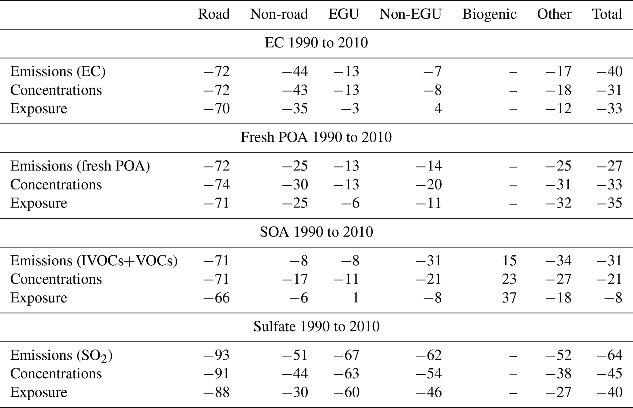
The changes in fresh POA are a little more interesting because it is treated as semi-volatile and reactive in PMCAMx. For all US sources, the reduction in concentrations is a little higher than that of the emissions (Table 3). For example, a 25 % reduction in POA emissions of non-road POA is predicted to have resulted in a 30 % reduction in the POA concentrations. This difference is due mostly to the nonlinear nature of the partitioning of these emissions between the gas and particulate phases. As the emissions are reduced, the corresponding OA concentrations are reduced, and more of the organic material is transferred to the gas phase to maintain equilibrium. This additional evaporation leads to an additional reduction in the POA concentrations. This is the case for all the sources, so the 27 % reduction in POA emissions corresponds according to PMCAMx to a 33 % average reduction in POA concentrations. The reduction in exposure is, in absolute terms, a little less than that of the concentrations for the same reasons as for EC. This difference is small (−74 % versus −71 %) for road transport but more significant for sources located outside urban centers (e.g., for EGU it is −13 % for concentrations and −6 % for exposure).
The reductions predicted by PMCAMx for SOA (aSOA + bSOA) concentrations are far more complex than those of fresh POA, since the formation of secondary organic species involves nonlinear processes such as partitioning, dependence on oxidant levels, NOx dependence of the yields, and the complexity of the chemical aging. Overall, PMCAMx predicts that the reductions in exposure are less than the reductions in average concentrations over the US, which are also less than the reductions in the emissions of the anthropogenic volatile and intermediate volatility organic compounds. One explanation for this behavior is that the simultaneous decreases in NOx levels have led to increased SOA formation yields. A second factor is the time required for the formation of SOA, especially when multiple generations of reactions are required. The result of this time delay is that SOA is often produced away from its sources located in high urban density areas. The reasons for this complex behavior will be analyzed in detail in future work.
The predicted reductions in sulfate concentrations are less than the reductions in emissions due mainly to the nonlinearity of the aqueous-phase conversion of SO2 to sulfate (Seinfeld and Pandis, 2016) (Table 3). Such nonlinearity has been predicted also in past CTM applications (Karydis et al., 2007; Tsimpidi et al., 2007). Taking into account the transport of some of the sulfate from areas outside of the US, the model predicts that the 64 % reduction in SO2 emissions has resulted in a 45 % reduction in the sulfate concentration on average. The reduction in exposure is a little less, 40 % on average, because both the major sources of SO2 are located and the higher reductions in sulfate take place, according to PMCAMx, away from the major urban centers.
4.5 Distribution of population exposure to PM2.5 from different sources
We have calculated the percentage of people exposed to different PM2.5 concentrations from the major sources (“other”, “EGUs”, “road transport”) for the three different periods. Almost half of the US population was exposed to PM2.5 concentrations above 20 µg m−3 in 1990. A decade later this percentage was less than 20 % and close to zero during 2010 (Fig. 9a). During 1990, almost 90 % of the US population was exposed to PM2.5 concentrations above 10 µg m−3, the suggested annual mean by the World Health Organization (WHO, 2006). This percentage was reduced to 83 % in 2001 and 70 % in 2010 (Figs. 9a and S2h).
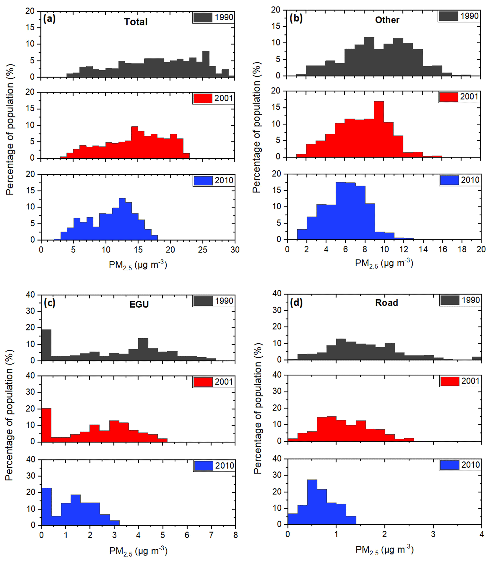
Figure 9Distributions of population exposed to annual average PM2.5 during 1990 (grey), 2001 (red), and 2010 (blue) and for the dominant sources of PM2.5: (a) total PM2.5 (all sources), (b) other, (c) EGU, and (d) road transport.
The predicted distribution of the population exposed to PM2.5 from the “other” source in 1990 covered a wide range extending from approximately 1 to 16 µg m−3. The exposure from these sources was reduced significantly in the following years, mainly due to the reductions in the emissions of paved/unpaved road dust, prescribed burning, and industrial emissions (Xing et al., 2013). The average emissions from wildfires did not change appreciably, but this distribution was sharper in 2010, with maximum percentages of people exposed appearing for PM2.5 concentrations ranging from 5 to 8 µg m−3. The random spatial variation of biomass burning sources can affect areas with different population densities.
The exposure of the population to primary and secondary PM2.5 from EGUs has dramatically decreased (Fig. 9c). In 1990, according to PMCAMx, 56 % of the US population was exposed to more than 3 µg m−3 from this source. This percentage was reduced to 39 % in 2001 and to 2 % in 2010. For the threshold of 5 µg m−3, the reduction was from 18 % in 1990 to 1 % in 2001 and to practically zero in 2010.
Similarly, significant decreases are predicted for road transport PM2.5. While in 1990 79 % of the population was exposed to levels exceeding 1 µg m−3, this percentage was 58 % in 2001 and 18 % in 2010 (Fig. 9d). The corresponding changes for 2 µg m−3 were from 27 % (1990) to 8 % (2001) and to zero (2010).
4.6 Predicted spatial changes in concentrations
We calculated the predicted changes in annual average concentrations between 1990 and 2010 for the main PM2.5 components. Figure S3 shows the reductions in EC concentrations from 1990 to 2010. The reductions in the EC emissions resulted in total reductions in the average concentrations of around 30 % in the 20-year period. Reductions above 20 % are predicted not only in the large urban areas, but also in large regions in both the eastern and western US.
Average organic aerosol levels were reduced according to PMCAMx by close to 1.5 µg m−3 from 1990 to 2010 in a wide area extending from the Great Lakes to Tennessee but also in parts of the eastern seaboard (Fig. S4). These reductions correspond to 35 %–45 % of the OA in both the NE and California.
From 1990 to 2010, sulfate was reduced by 50 %–60 % in the part of the country to the east of the Mississippi. The corresponding reductions in the middle of the country and in the western states from 1990 to 2010 were in the 20 %–30 % range for the relatively low sulfate levels in these regions (Fig. S5). These simulations suggest that the eastern US has benefited more both in an absolute and in a relative sense from these reductions in SO2 emissions.
We also compared the predicted and observed concentration changes, using the Pearson correlation coefficient and the average percentage differences, summarized in Table 4. Also, as far as the exposure changes are concerned, because of the way that exposure is defined (concentration times population) and the population is measured, the evaluation metrics of our exposure predictions are exactly the same as the evaluation metrics of our concentration predictions. For the first two cases (1990 to 2001 and 1990 to 2010) there were only a few measurements available for 1990. The model reproduces quite well the predicted changes against the observed changes for PM2.5 and its components (Fig. S6).
Table 4Average observed and predicted PM percentage changes and Pearson's correlation coefficient calculated for each comparison case.
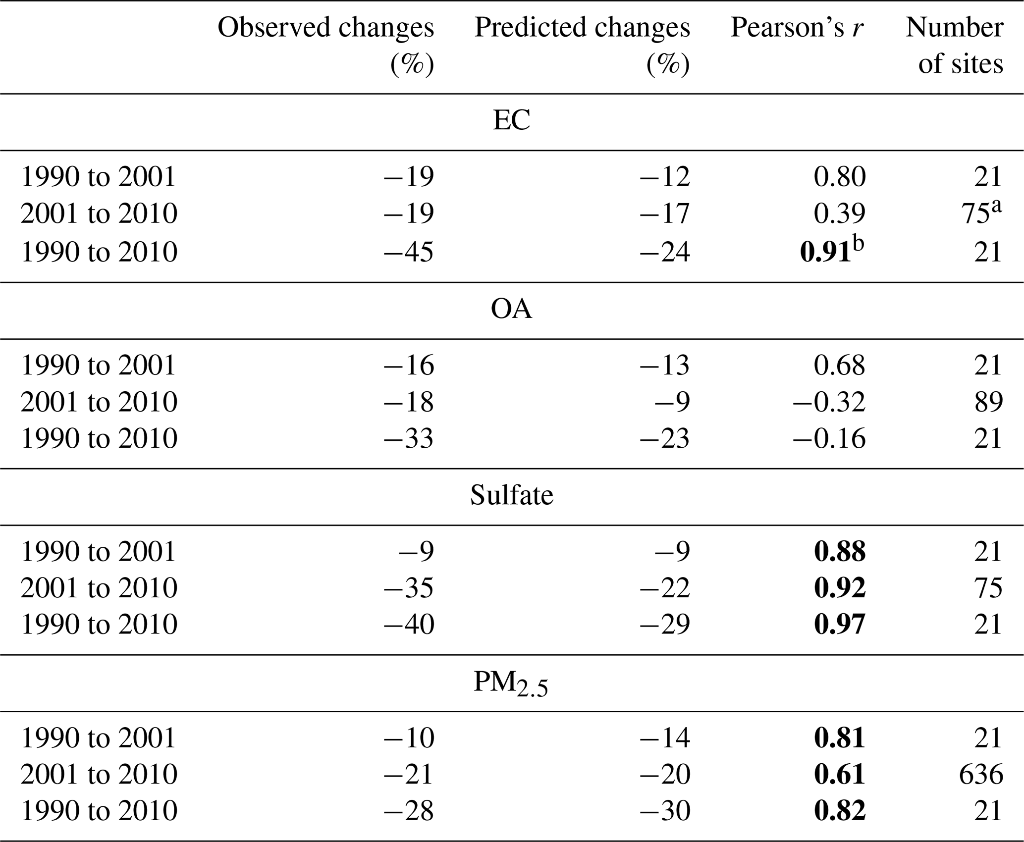
a Fourteen CSN sites reporting increases in EC, probably due to the change in the measurement protocol in the 2007–2009 period, have been excluded from this analysis. b The correlations in bold are statistically significant for a significance level of 5 %.
For EC, the correlation was high between 1990 and 2001, with r=0.80, and between 1990 and 2010, with r=0.91. However, the analysis for the changes up to 2010 is complicated by the change in the EC measurement protocol in several CSN sites in the period from 2007 to 2010. The change from the thermal optical transmittance (TOT) to the thermal optical reflectance (TOR) resulted in small increases in the reported EC that were of similar magnitude to the predicted changes due to the emission reductions. To partially address this issue, we do not include in the analysis the results from 14 CSN sites which reported increases in the EC from 2001 to 2010. Excluding these sites, r=0.39 is calculated (Table 4). The data points from these sites can be seen in the lower triangle of Fig. S6. The reduced r for 2001–2010 is probably due, at least partially, to this uncertainty in the measured changes.
The predicted average change in OA in the measurement sites from 1990 to 2001 was −13 %, in good agreement with the observed −16 % in the same locations. The predicted changes were reasonably well correlated (r=0.68) with the measured ones during this decade. However, the model performance during the next decade (2001–2010) deteriorates as it underpredicts on average the changes (predicted −9 % versus observed −18 %), and the changes are not correlated with each other in space. Additional analysis suggested that, while the model does a reasonable job reproducing the changes in the western half of the country and the northeastern quarter, it overpredicts the OA concentration in 2010 and thus underpredicts the reductions in the southeastern US. Our analysis also suggests that this is mainly due to an overprediction of the biogenic SOA in this part of the country. This is consistent with the anomalous predicted increase in biogenic SOA from 2001 to 2010 in the southeastern US (Figs. 7 and S1). This interesting discrepancy regarding the predicted and observed changes in biogenic SOA will be analyzed in detail in a subsequent paper.
For sulfate, the model reproduced well the observed changes for the three comparison periods, with Pearson's correlation coefficient r=0.88 from 1990 to 2001, 0.97 from 1990 to 2010, and 0.92 from 2001 to 2010 (Table 4). Despite the nonlinearity in the behavior of sulfate, the average predicted and observed percentage changes were consistent for the three comparison periods.
Finally, for PM2.5 the model reproduces well the observed changes for the three comparison periods with r=0.81 (from 1990 to 2001), 0.82 (from 1990 to 2010), and 0.61 (from 2001 to 2010). The average percentage changes for the observations and the predictions were close for all the cases (Table 4).
The CTM, PMCAMx, was used to simulate the changes in source contributions to PM2.5 and its components over 2 decades, accounting for changes in emissions and meteorology with internally consistent methods. Biomass burning and “other” sources, primarily including construction processes, mining, agriculture, waste disposal, and other miscellaneous sources, contributed approximately half of the total (primary and secondary) PM2.5 during the examined 20-year period. The corresponding average PM2.5 concentration levels due to this group of sources were reduced by 33 % from 1990 to 2010. EGUs were the second most important source of PM2.5; the corresponding ambient PM2.5 levels have been reduced by 55 % and their contribution to the total from 16 % to 11 %. On-road transport was the third most important source of PM2.5. The total average PM2.5 from this source was reduced by 59 %, while their contribution to the average PM2.5 levels has been reduced from 8 % to 5 %.
OA was a significant fraction of PM2.5. Biomass burning included in the “other” sources was the most important source of OA, with fractional contributions varying from 38 % to 52 % depending on the region. Biogenic SOA was the second dominant component of OA, with contributions ranging from 6 % to 22 % in the southern US.
The relationship between the changes in concentrations and changes in exposure is determined by the spatial distributions of these two changes. The more similar these distributions are, the closer the corresponding changes. The reduction in exposure was less than the reduction in emissions (or concentrations) for sources that are located away from densely populated regions (non-road transport and non-EGUs) due to the spatial non-uniformity of the corresponding PM2.5 reductions. For example, sulfate human exposure by non-EGU sources was reduced by 46 % from 1990 to 2010, while the corresponding reduction in emissions was 62 %.
From 1990 to 2010, the reduction in human exposure to EC was 33 %, to fresh POA 35 %, to sulfate 40 %, and to SOA (both anthropogenic and biogenic) 8 %. The reduction in EC was mostly due to the 72 % reduction in on-road EC emissions and the reduction in sulfate due to the 67 % reduction in SO2 emissions from EGUs.
Considering that the US population increased by almost 24 % from 1990 to 2010, the fact that the total population exposure to PM was reduced in most areas indicates that the emission reductions were sufficient to overcome this effect. The decreases in personal exposure have been higher than those of the total population exposure.
During the 20-year-long examined period, the fraction of the US population exposed to average PM2.5 concentrations above 20 µg m−3 decreased from approximately 50 % to close to zero. In 1990, 12 % of the US population was exposed to PM2.5, concentrations lower than the suggested annual mean by the WHO (10 µg m−3). This fraction increased to 30 % in 2010.
PMCAMx reproduced the annual average concentrations of PM2.5 with fractional error less than 30 % for the three simulation periods. The corresponding fractional biases were 16 % for 1990 and 5 % for both 2001 and 2010. The model also reproduces well the average reduction in PM2.5 in the measurement sites; the measured reduction was 28 %, while the model predicts a reduction of 30 %. A model weakness that requires additional investigation is its tendency to predict an increase in the biogenic SOA from 2001 to 2010 that appears inconsistent with the observations.
The code and simulation results are available upon request (spyros@chemeng.upatras.gr).
The supplement related to this article is available online at: https://doi.org/10.5194/acp-21-17115-2021-supplement.
KS performed the PMCAMx and PSAT simulations, analyzed the results, and wrote the manuscript. PGR prepared the anthropogenic emissions and other inputs for the simulations. BD performed MEGAN simulations and analyzed the results; EK performed and evaluated the WRF simulations; IK set up the WRF simulations and assisted in the preparation of the meteorological inputs. CH analyzed the simulation output. SNP and PJA designed and coordinated the study and helped in the writing of the paper. All the authors reviewed and commented on the manuscript.
The contact author has declared that neither they nor their co-authors have any competing interests.
Publisher’s note: Copernicus Publications remains neutral with regard to jurisdictional claims in published maps and institutional affiliations.
This work was supported by the Center for Air, Climate, and Energy Solutions (CACES), which was supported under assistance agreement no. R835873 awarded by the U.S. Environmental Protection Agency and the Horizon-2020 Project REMEDIA of the European Union under grant agreement no. 874753.
This paper was edited by Qiang Zhang and reviewed by two anonymous referees.
Beckerman, B. S., Jerrett, M., Serre, M., Martin, R. V., Lee, S.-J., van Donkelaar, A., Ross, Z., Su, J., and Burnett, R. T.: A hybrid approach to estimating national scale spatiotemporal variability of PM2.5 in the contiguous United States, Environ. Sci. Technol., 47, 7233–7241, 2013.
Donahue, N. M., Robinson, A. L., Stanier, C. O., and Pandis, S. N.: Coupled partitioning, dilution, and chemical aging of semivolatile organics, Environ. Sci. Technol., 40, 2635–2643, 2006.
Eeftens, M., Beelen, R., de Hoogh, K., Bellander, T., Cesaroni, G., Cirach, M., Declercq, C., Delele, A., Dons, E., and de Nazelle, A.: Development of land use regression models for PM2.5 absorbance, PM10 and PMCoarse in 20 European study areas, results of the ESCAPE Project, Environ. Sci. Technol., 46, 11195–11205, 2012.
Emery, C., Liu, Z., Russell, A. G., Odman, M. T., Yarwood, G., and Kumar, N.: Recommendations on statistics and benchmarks to assess photochemical model performance, J. Air Waste Manage., 67, 582–598, 2017.
Environ: Comprehensive Air Quality Model with Extensions Version 4.40, Users Guide, ENVIRON Int. Corp., Novato, CA, available at: http://www.camx.com (last access: November 2020), 2006.
Fountoukis, C., Racherla, P. N., Denier van der Gon, H. A. C., Polymeneas, P., Charalampidis, P. E., Pilinis, C., Wiedensohler, A., Dall'Osto, M., O'Dowd, C., and Pandis, S. N.: Evaluation of a three-dimensional chemical transport model (PMCAMx) in the European domain during the EUCAARI May 2008 campaign, Atmos. Chem. Phys., 11, 10331–10347, https://doi.org/10.5194/acp-11-10331-2011, 2011.
Gan, C.-M., Hogrefe, C., Mathur, R., Pleim, J., Xing, J., Wong, D., Gilliam, R., Pouliot, G., and Wei, C.: Assessment of the effects of horizontal grid resolution on long-term air quality trends using coupled WRF-CMAQ simulations, Atmos. Environ., 132, 207–216, 2016.
Gilliam, R. C. and Pleim, J. E.: Performance assessment of new land surface and planetary boundary layer physics in the WRF-ARW, J. Appl. Meteorol. Clim., 49, 760–774, 2010.
Hogrefe, C., Pouliot, G., Wong, D., Torian, A., Roselle, S., Pleim, J., Mathur, R.: Annual application and evaluation of the online coupled WRF-CMAQ system over North America under AQMEII phase 2, Atmos. Environ., 115, 683–694, 2015.
Iacono, M. J., Delamere, J. S., Mlawer, E. J., Shephard, M. W., Clough, S. A., and Collins, W. D.: Radiative forcing by long-lived greenhouse gases: Calculations with the AER radiative transfer models, J. Geophys. Res., 113, 2–9, 2008.
IMPROVE: IMPROVE Data Guide. Univ. of California, Davis, available at: https://vista.cira.colostate.edu/improve/Publications/OtherDocs/IMPROVEDataGuide/IMPROVEDataGuide.htm (last access: September 2020), 1995.
Jiang, X., Guenther, A., Potosnak, M., Geron, C., Seco, R., Karl, T., Kim, S., Gu, L., and Pallardy, S.: Isoprene emission response to drought and the impact on global atmospheric chemistry, Atmos. Environ., 183, 69–83, 2018.
Jin, X., Fiore A. M., Civerolo, K., Bi, J., Liu, Y., Donkelaar, A., Martin, R. V., Al-Hamdan, M., Zhang, Y., Insaf, T. Z., Kioumourtzoglou, M., He, M. Z., and Kinney, P. L.: Comparison of multiple PM2.5 exposure products for estimating health benefits of emission controls over New York State, USA, Environ. Res. Lett., 14, 084023, https://doi.org/10.1088/1748-9326/ab2dcb, 2019.
Kain, J. S.: The Kain–Fritsch convective parameterization: An update, J. Appl. Meteorol., 43, 170–181, 2004.
Karamchandani, P., Vijayaraghavan, K., and Yarwood, G.: Sub-grid scale plume modeling, Atmosphere, 2, 389–406, 2011.
Karydis, V. A., Tsimpidi, A. P., and Pandis, S. N.: Evaluation of a three-dimensional chemical transport model (PMCAMx) in the eastern United States for all four seasons, J. Geophys. Res., 112, D14211, https://doi.org/10.1029/2006JD007890, 2007.
Karydis, V. A., Tsimpidi, A. P., Fountoukis, C., Nenes, A., Zavala, M., Lei, W., Molina, L. T., and Pandis, S. N.: Simulating the fine and coarse inorganic particulate matter concentrations in a polluted megacity, Atmos. Environ., 44, 608–620, 2010.
Lane, T. E., Donahue, N. M., and Pandis, S. N.: Effect of NOx on secondary organic aerosol concentrations, Environ. Sci. Technol., 42, 6022–6027, 2008.
Li, L., Wu, A. H., Cheng, I., Chen, J.-C., and Wu, J.: Spatiotemporal estimation of historical PM2.5 concentrations using PM10 meteorological variables, and spatial effect, Atmos. Environ., 166, 182–191, 2017a.
Li, C., Martin, R. V., van Donkelaar, A., Boys, B. L., Hammer, M. S., Xu, J.-W., Marais, E. A., Reff, A., Strum, M., Ridley, D. A., Crippa, M., Brauer, M., and Zhang, Q.: Trends in chemical composition of global and regional population-weighted fine particulate matter estimated for 25 years, Environ. Sci. Technol., 51, 11185–11195, 2017b.
Ma, Z., Hu, X., Sayer, A. M., Levy, R., Zhang, Q., Xue, Y., Tong, S., Bi, J., Huang, L., and Liu, Y.: Satellite-based spatiotemporal trends in PM2.5 concentrations: China, 2004–2013, Environ. Health Persp., 124, 184–192, 2016.
Meng, J., Li, C., Martin, R. V., van Donkelaar, A., Hystad, P., and Brauer, M.: Estimated long-term (1981–2016) concentrations of ambient fine particulate matter across North America from chemical transport modeling, satellite remote sensing and ground-based measurements, Environ. Sci. Technol., 53, 5071–5079, 2019.
Milando, C., Huang, L., and Batterman, S.: Trends in PM2.5 emissions, concentrations and apportionments in Detroit and Chicago, Atmos. Environ., 129, 197–209, 2016.
Morris, R. E., McNally, D. E., Tesche, T. W., Tonnesen, G., Boylan, J. W., and Brewer, P.: Preliminary Evaluation of the Community Multiscale Air Quality Model for 2002 over the Southeastern United States, J. Air Waste Manage., 55, 1694–1708, 2005.
Morrison, H., Thompson, G., and Tatarskii, V.: Impact of cloud microphysics on the development of trailing stratiform precipitation in a simulated squall line: Comparison of one- and two-moment schemes, Mon. Weather Rev., 137, 991–1007, 2008.
Murphy, B. N. and Pandis, S. N.: Simulating the formation of semivolatile primary and secondary organic aerosol in a regional chemical transport model, Environ. Sci. Technol., 43, 4722–4728, 2009.
Murphy, B. N. and Pandis, S. N.: Exploring summertime organic aerosol formation in the Eastern United States using a regional-scale budget approach and ambient measurements, J. Geophys. Res., 115, D24216, https://doi.org/10.1029/2010JD014418, 2010.
Murphy, S. L., Xu, J., and Kochanek, K. D.: Deaths: Final Data for 2010, Division of Vital Statistics National Vital Statistics Reports, 61, 4, 2013.
Nenes, A., Pandis, S. N., and Pilinis, C.: ISORROPIA: a new thermodynamic equilibrium model for multiphase multicomponent inorganic aerosols, Aq. Geochem., 4, 123–152, 1998.
Nopmongcol, U., Alvarez, Y., Jung, J., Grant, J., Kumar, N., and Yarwood, G.: Source contributions to United States ozone and particulate matter over five decades from 1970 to 2020, Atmos. Environ., 167, 116–128, 2017.
Pandis, S. N., Wexler, A. S., and Seinfeld, J. H.: Secondary organic aerosol formation and transport – II. Predicting the ambient secondary organic aerosol size distribution, Atmos. Environ., 27, 2403–2416, 1993.
Pleim, J. E.: A Combined local and nonlocal closure model for the atmospheric boundary layer. Part I: Model description and testing, J. Appl. Meteorol. Clim., 46, 1383–1395, 2007a.
Pleim, J. E.: A combined local and nonlocal closure model for the atmospheric boundary layer. Part II: Application and evaluation in a mesoscale meteorological model, J. Appl. Meteorol. Clim., 46, 1396–1409, 2007b.
Posner, L. N., Theodoritsi, G., Robinson, A., Yarwood, G., Koo, B., Morris, R., Mavko, M., Moore, T., and Pandis, S. N.: Simulation of fresh and chemically-aged biomass burning organic aerosol, Atmos. Environ., 196, 27–37, 2019.
Rogers, R. E., Deng, A., Stauffer, D. R., Gaudet, B. J., Jia, Y., Soong, S. T., and Tanrikulu, S.: Application of the weather research and forecasting model for air quality modeling in the San Francisco bay area, J. Appl. Meteorol. Clim., 52, 1953–1973, 2013.
Seinfeld, J. H. and Pandis, S. N.: Atmospheric Chemistry and Physics, 3rd Edn., John Wiley and Sons, New Jersey, USA, 2016.
Sindelarova, K., Granier, C., Bouarar, I., Guenther, A., Tilmes, S., Stavrakou, T., Müller, J.-F., Kuhn, U., Stefani, P., and Knorr, W.: Global data set of biogenic VOC emissions calculated by the MEGAN model over the last 30 years, Atmos. Chem. Phys., 14, 9317–9341, https://doi.org/10.5194/acp-14-9317-2014, 2014.
Skyllakou, K., Murphy, B. N., Megaritis, A. G., Fountoukis, C., and Pandis, S. N.: Contributions of local and regional sources to fine PM in the megacity of Paris, Atmos. Chem. Phys., 14, 2343–2352, https://doi.org/10.5194/acp-14-2343-2014, 2014.
Skyllakou, K., Fountoukis, C., Charalampidis, P., and Pandis, S. N.: Volatility-resolved source apportionment of primary and secondary organic aerosol over Europe, Atmos. Environ., 167, 1–10, 2017.
Tessum, C. W., Apte, J. S., Goodkind, A. L., Muller, N. Z., Mullins, K. A., Paolella, D. A., Polasky, S., Springer, N. P., Thakrar, S. K., Marshall, J. D., and Hill, J. D.: Inequity in consumption of goods and services adds to racial–ethnic disparities in air pollution exposure, P. Natl. Acad. Sci. USA, 116, 6001–6006, 2019.
Tsimpidi, A. P., Karydis, V. A., Pandis, S. N.: Response of Inorganic Fine Particulate Matter to Emission Changes of Sulfur Dioxide and Ammonia: The Eastern United States as a Case Study, J. Air Waste Manage., 57, 1489–1498, 2007.
Tsimpidi, A. P., Karydis, V. A., Zavala, M., Lei, W., Molina, L., Ulbrich, I. M., Jimenez, J. L., and Pandis, S. N.: Evaluation of the volatility basis-set approach for the simulation of organic aerosol formation in the Mexico City metropolitan area, Atmos. Chem. Phys., 10, 525–546, https://doi.org/10.5194/acp-10-525-2010, 2010.
US Census Bureau: Population Estimates, available at: https://www.census.gov, last access: November 2020.
US EPA (U.S. Environmental Protection Agency): User Guide: Air Quality System, Report, Research Triangle Park, N. C., available at: https://www.epa.gov/ttn/airs/airsaqs/ manuals/AQSUserGuide.pdf (last access: September 2020), 2002.
US EPA (U.S. Environmental Protection Agency): Benefits and Costs of the Clean Air Act 1990–2020, Report Documents and Graphics, available at: https://www.epa.gov/sites/default/files/2015-07/documents/summaryreport.pdf (last access: August 2021), 2011.
Wagstrom, K. M., Pandis, S. N., Yarwood, G., Wilson, G. M., and Morris, R. E.: Development and application of a computationally efficient particulate matter apportionment algorithm in a three-dimensional chemical transport model, Atmos. Environ., 42, 5650–5659, 2008.
Wagstrom, K. M. and Pandis, S. N.: Source receptor relationships for fine particulate matter concentrations in the Eastern United States, Atmos. Environ., 45, 347–356, 2011a.
Wagstrom, K. M. and Pandis, S. N.: Contribution of long-range transport to local fine particulate matter concerns, Atmos. Environ., 45, 2730–2735, 2011b.
Walker, S. E., Slordal, L. H., Guerreiro, C., Gram, F., and Gronskei, K. E.: Air pollution exposure monitoring and estimation part II. Model evaluation and population exposure, J. Environ. Monitor., 1, 321–326, 1999.
WHO: Air Quality Guidelines for Particulate Matter, Ozone, Nitrogen Dioxide and Sulfur Dioxide, GLOBAL Update 2005, Summary of Risk Assessment, World Health Organization (WHO/SDE/PHE/OEH/06.02), 2006.
Xing, J., Pleim, J., Mathur, R., Pouliot, G., Hogrefe, C., Gan, C.-M., and Wei, C.: Historical gaseous and primary aerosol emissions in the United States from 1990 to 2010, Atmos. Chem. Phys., 13, 7531–7549, https://doi.org/10.5194/acp-13-7531-2013, 2013.
Xiu, A. and Pleim, J. E.: Development of a land surface model. Part I: Application in a Mesoscale Meteorological Model, J. Appl. Meteorol., 40, 192–209, 2002.
Yarwood, G., Rao, S., Yocke, M., and Whitten, G. Z.: Updates to The Carbon Bond Chemical Mechanism, Research Triangle Park, 2005.
Zakoura, M. and Pandis, S. N: Improving fine aerosol nitrate predictions using a Plume-in-Grid modeling approach, Atmos. Environ., 215, 116887, https://doi.org/10.1016/j.atmosenv.2019.116887, 2019.