Transport-driven aerosol differences above and below the canopy of a mixed deciduous forest

Exchanges of energy and mass between the surrounding air and plant surfaces occur below, within, and above a forest's vegetative canopy. The canopy also can lead to vertical gradients in light, trace gases, oxidant availability, turbulent mixing, and properties and concentrations of organic aerosol (OA). In this study, a high-resolution time-of-flight aerosol mass spectrometer was used to measure non-refractory submicron aerosol composition and concentration above (30 m) and below (6 m) a forest canopy in a mixed deciduous forest at the Program for Research on Oxidants: PHotochemistry, Emissions, and Transport tower in northern Michigan during the summer of 2016. Three OA factors are resolved using positive matrix factorization: more-oxidized oxygenated organic aerosol (MO-OOA), isoprene-epoxydiol-derived organic aerosol (IEPOX-OA), and 91Fac (a factor characterized with a distinct fragment ion at $m/z$ 91) from both the above- and the below-canopy inlets. MO-OOA was most strongly associated with long-range transport from more polluted regions to the south, while IEPOX-OA and 91Fac were associated with shorter-range transport and local oxidation chemistry. Overall vertical similarity in aerosol composition, degrees of oxidation, and diurnal profiles between the two inlets was observed throughout the campaign, which implies that rapid in-canopy transport of aerosols is efficient enough to cause relatively consistent vertical distributions of aerosols at this scale. However, four distinct vertical gradient episodes are identified for OA, with vertical concentration differences (above-canopy minus below-canopy concentrations) in total OA of up to 0.8 µg m⁻³, a value that is 42 % of the campaign average OA concentration of 1.9 µg m⁻³. The magnitude of these differences correlated with concurrent vertical differences in either sulfate aerosol or ozone. These differences are likely driven by a combination of long-range transport mechanisms, canopy-scale mixing, and local chemistry. These results emphasize the importance of including vertical and horizontal transport mechanisms when interpreting trace gas and aerosol data in forested environments.

1 Introduction

Aerosols play a key role in the energy balance of the Earth's climate system by scattering and absorbing incoming solar radiation and by impacting cloud lifetime and reflectivity (IPCC, 2007). These climatic effects depend strongly on the chemical speciation of the aerosol particles. On average, approximately 20 %–90 % of submicron aerosol mass worldwide has been predicted to be organic material (Kanakidou et al., 2005), and this is supported by field studies in a variety of urban, urban downwind, and rural locations across the Northern Hemisphere (Jimenez et al., 2009; Zhang et al., 2007). The bulk of this organic material is thought to be secondary organic aerosol (SOA), which is formed in the atmosphere by the reaction of volatile organic compounds (VOCs) with oxidants such as the hydroxyl radical (OH), ozone (O₃), the nitrate radical, and chlorine atoms, with the resulting products then partitioning to the particle phase.

Precursor VOCs that contribute to SOA formation are emitted from both anthropogenic and biogenic sources. Biogenic VOCs (BVOCs) are primarily emitted into the atmosphere from terrestrial vegetation, and on a global scale, emissions of BVOCs exceed those of anthropogenic VOCs (Fehsenfeld et al., 1992; Guenther et al., 2000, 1995). Major SOA precursor BVOCs include isoprene (C₅H₈) and terpenes. To date, more than 5000 terpene compounds have been identified, including monoterpenes (C₁₀), sesquiterpenes (C₁₅), and diterpenes (C₂₀) (Geron et al., 2000). However, factors such as the addition of functional groups (aldehydes, alcohols, carboxylic acids, alkyl nitrate, etc.) and the wide variety of possible reaction pathways rapidly increase the number of relevant atmospheric VOCs beyond what is initially emitted (Goldstein and Galbally, 2007).

If other loss processes, including deposition, were not considered, the final atmospheric fate of the carbon associated with BVOCs would be oxidation to carbon dioxide. However, partitioning of oxidation products to the aerosol phase as SOA interrupts this oxidation sequence. Partitioning of VOC oxidation products between the gas and aerosol phases depends on multiple factors such as the phase and concentration of pre-existing primary OA (POA) or SOA, particulate-phase SOA reactions, and the presence of aerosol liquid water (ALW) (Seinfeld and Pandis, 2006). As a result of the large number of precursor VOCs, the highly non-linear oxidation chemistry, and the presence of multiple aerosol phases in the atmosphere, SOA formation is complex and relatively poorly understood (Goldstein and Galbally, 2007).

The physical environment strongly impacts these chemical SOA formation processes. For example, in forested areas in which BVOC emissions are prevalent, the exchanges of energy and mass between the forest and the atmosphere are influenced by the forest's vegetation canopy. Absorption of light by a canopy can diminish the amount of radiation that is received below the canopy, influencing photolysis rates of photolabile species (Baldocchi et al., 1995; Brown et al., 2005; Fuentes et al., 2007; Makar et al., 2017; Schulze et al., 2017) and oxidant availability (Fuentes et al., 2007). Loss of BVOC oxidation products to deposition within the canopy also has been found to be an important factor in determining the oxidative capacity of a forested environment (Pugh et al., 2010).

Vertical transport, also influenced by the canopy, likewise impacts the concentrations of BVOC and SOA in forested environments. Roughness elements created by the leaves, branches, and stems in a dense vegetative canopy combined with above-canopy wind shear lead to coherent structures (Finnigan, 2000). These turbulent flow structures contribute to the fluxes of heat, energy, and matter in forest canopies (Thomas and Foken, 2007). The physical motion of coherent structures occurs via two main mechanisms: upward “bursts”, in which air is ejected upward from the canopy into the atmosphere, and downward “sweeps”, in which air is directed downward from the atmosphere into the canopy. Vertically resolved sonic anemometer measurements, which provide temperature and three-dimensional wind velocity components at each vertical measurement location, can be used to derive in-canopy mixing metrics.

The relative magnitudes of timescales for turbulent transport and chemical processing govern how trace compounds are distributed within the canopy (Baldocchi et al., 1995; Fuentes et al., 2007; Steiner et al., 2011). A modeling study by Gao et al. (1993) found that in-canopy chemical processing of isoprene occurs on a much longer timescale than turbulent transport, making in-canopy reactions less important compared to the turbulent transport and emission of isoprene in determining its in-canopy concentrations. On the other hand, for compounds with an estimated chemical loss timescale that is roughly equivalent to the timescales of turbulent transport (e.g., O₃-initiated oxidation of the sesquiterpene β-caryophyllene), rapid in-canopy chemical loss could dominate (Stroud et al., 2005). Furthermore, partitioning to the aerosol phase was inferred as a potential reason for observations of decreased mixing ratios of oxidation products of very reactive BVOCs in a ponderosa pine forest canopy (Holzinger et al., 2005).

Several studies have attempted to model vertical profiles of trace gases and aerosols in a forest canopy considering both chemistry and turbulent transport. Bryan et al. (2012) found that forest canopy–atmosphere interactions were highly sensitive to turbulent mixing parameterizations during a field campaign in northern Michigan. Differences in highly reactive BVOCs and BVOC oxidation products have been estimated above and below the canopy in modeling and measurement efforts (Alwe et al., 2019; Ashworth et al., 2015; Holzinger et al., 2005; Schulze et al., 2017; Stroud et al., 2005; Wolfe and Thornton, 2011). Schulze et al. (2017) found that rapid through-canopy transport (minimum in-canopy residence time of 10 min) leads to relatively consistent simulated above- and below-canopy SOA composition and concentration.

Because in-canopy mixing plays a role in the vertical distribution of trace gases and aerosols in a forest canopy, vertical differences in OA components and other inorganic aerosol species such as sulfate (SO₄) could be caused by the degree of mixing between the above- and below-canopy environments. During the Program for Research on Oxidants: PHotochemistry, Emissions, and Transport (PROPHET)–Community Atmosphere-Biosphere Interactions Experiment (CABINEX) 2009 campaign, the degree of atmosphere–canopy coupling between the above-canopy atmosphere and the forest was analyzed by Steiner et al. (2011). In this study, the degree of coupling was calculated using the ratio of the kinematic heat flux above the canopy to the kinematic heat flux in the upper canopy. Opposing kinematic heat flux directions (negative ratios) imply that the below-canopy environment is uncoupled from the atmosphere. In 2009, coupling conditions ranged between strong coupling (greater than zero but less than the threshold value defined by the slope of a regression between the two heat fluxes), weak coupling (greater than the defined threshold value), and uncoupled (negative). Uncoupled conditions occurred most commonly in the early morning hours between 04:00 and 08:00 local time. This set of hours represents approximately 30 % of every day over the whole 2009 study period. This suggests that early morning hours may contribute to more instances of uncoupled canopy–atmosphere conditions but that coupling between the forest canopy and the atmosphere occurs a majority of the time (Steiner et al., 2011).

Past field studies, such as those above a tropical forest in Brazil and a temperate forest in California, found that in-canopy SOA formation, deposition, and thermal gradient effects on gas–particle partitioning all influence net OA fluxes (Farmer et al., 2013). In the same work, the authors found that oxygenated OA tended to be deposited in the canopy, whereas the forest canopy released less oxygenated OA. The source of OA fluxes between forests and the atmosphere has been associated with vertical turbulent transport between the forest atmosphere and the surface layer directly above the canopy; however, there have been few studies that have provided high-temporal-resolution measurements of both OA composition throughout a forest canopy and canopy mixing strength. In a mixed forest in Ontario, Canada, Gordon et al. (2011) found that the frequent occurrence of net upward aerosol flux was associated with decoupled canopy conditions where entrainment of particle-free air from above the canopy created a positive flux above the forest. On the other hand, Whitehead et al. (2010) found that the particle number concentration and submicron particle composition in the trunk space (i.e., below-canopy) and above-canopy environments showed minimal variation with height during the daytime due to stronger turbulence and mixing conditions. In light of these limited studies, there is a need for additional measurements and data to inform understanding of the exchange of aerosols between the forest and the atmosphere.

Recent work from PROPHET during the Atmospheric Measurements of Oxidants in Summer (AMOS) campaign in 2016 has indicated that flux of isoprene and monoterpenes at the canopy–atmosphere boundary represents over half of the net carbon flux, while oxygenated VOCs (OVOCs) constitute a majority of the species with detectable VOC fluxes (192 of the 236 species with identified molecular formulas). The authors report that the observed and modeled net carbon flux was upward (canopy emission) during the campaign in 2016 (Millet et al., 2018). Vertical gradients of BVOCs in this mixed forest environment vary greatly depending on canopy vegetation height, primary emission versus secondary production, and diurnal variability (Alwe et al., 2019). Correlation analysis of VOC vertical gradients suggests that formic acid (HCOOH) originates from secondary photochemical production. During the same campaign, distinct sample-to-sample variability in the molecular-level aerosol composition (73±8 %) was observed despite less variability in the elemental composition of the bulk OA, indicating the chemical complexity of functionalized OA at the site (Ditto et al., 2018).

Here, measurements using an Aerodyne high-resolution time-of-flight aerosol mass spectrometer (HR-ToF-AMS) are used to characterize ambient aerosol above and below the canopy in a mixed deciduous forest during the PROPHET–AMOS campaign in 2016, with the aim of evaluating quantitatively potential chemical and physical phenomena leading to observed differences between particulate matter above and below the forest canopy. These measurements provide data for validation of forest canopy–atmosphere exchange models and allow an assessment of turbulent transport in the forest canopy and the resulting impacts on above- and below-canopy SOA composition and concentration. These data could also assist in the determination of whether or not SOA is forming within the forest canopy.

2 Methods

2.1 Site description

Measurements were made during the PROPHET–AMOS 2016 campaign from 1–31 July 2016. The PROPHET site (45.55^∘ N, 84.78^∘ W) is situated in a temperate, mixed deciduous forest in the northern portion of Michigan's Lower Peninsula at the University of Michigan Biological Station (UMBS). The surrounding forest consists of aspens (60.9 %), northern hardwoods (16.6 %; maple, beech, birch, ash, and hemlocks), upland conifers (13.3 %; white and red pines), non-forest cover types (7.6 %; bracken ferns, grass, developed, and road), and northern red oak (1.6 %) (Cooper et al., 2001; Bergen and Dronova, 2007). The forests in this region are currently undergoing succession, where the dominant aspens have matured and are now being replaced by northern hardwoods and pines (Bergen and Dronova, 2007). It is expected that this new forest composition will shift BVOC emissions from an isoprene-dominated environment to one that is more influenced by monoterpenes (Toma and Bertman, 2012). The height of the forest canopy varies, but the mean canopy height is approximately 22.5 m (VanReken et al., 2015). The site's physical layout and site meteorology have been described elsewhere (Carroll et al., 2001; Cooper et al., 2001). The PROPHET site features a 31 m scaffolding tower, allowing measurements to be made at variable heights within and above the vegetation canopy.

Due to the sparse surrounding population, the PROPHET site at UMBS has minimal local anthropogenic influences. The closest major urban centers include Detroit, Michigan (350 km to the southeast, population 672 795); Milwaukee, Wisconsin (350 km to the southwest, population 595 047); and Chicago, Illinois (450 km to the southwest, population 2 704 958) (Carroll et al., 2001). The closest nearby towns include Pellston, Michigan (5 km to the west, population 828); Petoskey, Michigan (30 km to the southwest, population 5749); and Cheboygan, Michigan (30 km to the northeast, population 4726). Population totals are based on 2016 population estimates for cities and towns in the United States (US) from the US Census Bureau (US Census Bureau, 2018).

The mean temperature during the campaign was 20.6±4.6 ^∘C (mean ± 1 standard deviation), which is 3–4 ^∘C warmer than the mean temperature during the 2009 PROPHET–CABINEX campaign (16.9 ^∘C) (VanReken et al., 2015). Temperature conditions during this study are consistent with mean summertime temperatures from studies in 2008 and 2010 (Toma and Bertman, 2012) and with historical mean temperature data for the month of July from the Pellston Regional Airport (Fig. S1 in the Supplement). The mean relative humidity (RH) during the campaign was 73.8±17.5 %, which is similar to conditions during the CABINEX campaign (74.5±17.5 %) (VanReken et al., 2015). Winds recorded at the top of the PROPHET tower originated mostly from the west, southwest, and northwest (as shown in Fig. S2). The historical average precipitation according to the National Atmospheric Deposition Program (NADP) National Trends Network for the month of July from 1979–2015 for UMBS is 69.0 ± 37.8 mm. During the PROPHET–AMOS 2016 campaign, the total accumulated precipitation was 79.0 mm, indicating that precipitation at the site during the campaign was within 1 standard deviation of the historical July average (National Atmospheric Deposition Program, 2016).

2.2 Instrumentation and sampling

A summary of the trace gas measurements, instrumentation, and meteorological parameters on board the University of Houston–Rice University Mobile Air Quality Laboratory (MAQL) are summarized in Table S1 of the Supplement. Details and operation of the MAQL have been described previously in the literature (Leong et al., 2017; Wallace et al., 2018). The MAQL was situated approximately 10 m to the east of the PROPHET tower. A photograph of the MAQL in stationary sampling mode is shown in Fig. S3. Table S2 lists the measurements, measurement methods, and sampling heights of other participating institutions at PROPHET–AMOS 2016 during the campaign. Measurements are reported in local time (LT, eastern daylight time (EDT)) during the campaign.

2.2.1 Trace gases

Below-canopy trace gases including nitric oxide (NO), nitrogen dioxide (NO₂), total reactive nitrogen (NO_y), O₃, carbon monoxide (CO), and sulfur dioxide (SO₂) were measured from a common inlet on the sampling arm of the MAQL. Reported values of nitrogen oxides (NO_x) represent the sum of NO and NO₂, while reported values of NO_y include NO_x and its reservoir species. These measurements were taken at a height of 6 m above ground level (a.g.l.).

2.2.2 HR-ToF-AMS

The HR-ToF-AMS (Aerodyne Research Inc., USA) was used to measure non-refractory submicron particulate matter (NR-PM₁) from the MAQL; the measured composition includes OA, SO₄, nitrate (NO₃), ammonium (NH₄), and chloride (Chl). Detailed descriptions of the operation and principles of the HR-ToF-AMS have been provided elsewhere (DeCarlo et al., 2006). In brief, particles are sampled through a 100 µm critical orifice and are focused into a particle beam using an aerodynamic lens. After traversing a vacuum chamber, the particles in the beam impact onto a tungsten vaporizer heated to 600 ^∘C. The vapors formed are ionized by electron impact ionization at 70 eV. The resulting ions are detected using a high-resolution time-of-flight mass spectrometer. The HR-ToF-AMS was operated in a high-mass-sensitivity mode, referred to as the V mode. Ionization efficiency (IE) calibrations were performed at the beginning and end of the campaign using monodisperse 300 nm NH₄NO₃ particles. Gas-phase interferences were subtracted from the data based on the observed signal when ambient air was sampled through a filter. Filter zeros were run each day at varying times of day.

Sampling was performed from the raised 6 m inlet on the common sampling arm of the MAQL (below canopy) and from a 30 m inlet on the PROPHET tower (above canopy). Copper tubing was used for the sampling inlets, and each inlet was fitted with cyclones to remove particles larger than 2.5 µm in diameter. Prior to the HR-ToF-AMS critical orifice, air was sampled through a Nafion dryer to dry the sample flow. A three-way valve was used to alternate HR-ToF-AMS sampling between the above- and below-canopy inlets at 10 min intervals.

2.2.3 PTR-QiToF

Above-canopy mixing ratios and fluxes, along with in-canopy vertical gradients, were measured for a wide array of VOCs during PROPHET–AMOS 2016 by proton transfer reaction–quadrupole interface time-of-flight mass spectrometry (PTR-QiToF). A detailed description of the sampling configuration, calibration and zeroing procedures, humidity corrections, and instrumental performance during the campaign is provided by Alwe et al. (2019) and Millet et al. (2018). Briefly, six identical 45 m inlet lines (0.5 in. o.d., 0.375 in. i.d., PFA, each heated to 50 ^∘C) were installed on the PROPHET tower to sample from 34, 21, 17, 13, 9, and 5 m a.g.l. Sample flow was maintained at ∼ 40 standard L min⁻¹ (SLM) for the 34 m inlet line and at > 5–10 SLM for the others. Each hour, 30 min was spent sampling from the 34 m inlet to quantify above-canopy VOC mixing ratios and fluxes. The remainder of each hour was spent characterizing in-canopy vertical gradients by sequentially sampling from the other inlets (for 5 min apiece) followed by a 5 min instrumental blank.

2.3 HR-ToF-AMS data and positive matrix factorization analysis

Data analysis for HR-ToF-AMS data was performed in Igor Pro v6.37 using the SQUIRREL (SeQUential Igor data RetRiEvaL) v1.57 and PIKA (Peak Integration by Key Analysis) v1.16 analysis toolkits (DeCarlo et al., 2006). High-resolution mass spectral fitting was performed on HR-ToF-AMS V-mode data. Ratios such as the oxygen-to-carbon elemental ratio (O : C) and hydrogen-to-carbon elemental ratio (H : C) were determined according to the “improved-ambient” (IA) method (Canagaratna et al., 2015). The IA method uses specific ion fragments to correct for compositional biases, and this method has been shown to calculate accurately the elemental ratios of organic laboratory standards that are more representative of oxidized, ambient OA species (Canagaratna et al., 2015). The default values for relative IE were used for each of the following species: OA (1.4), SO₄ (1.2), NH₄ (4), NO₃ (1.1), and Chl (1.3), where values in parentheses refer to the ratio of the IE of the given species with respect to the value of the IE of NO₃ obtained during routine IE calibrations using NH₄NO₃.

To account for the effects of aerosol composition on the transmission efficiency of aerosols to the detection region of the HR-ToF-AMS, a chemical composition-dependent (and therefore time-dependent) collection efficiency (CDCE) was applied to the HR-ToF-AMS data (Middlebrook et al., 2012), which led to an campaign average CDCE of 0.77 ± 0.18. During the campaign, the HR-ToF-AMS time resolution was 40 s from 2 July 02:00 to 19 July 10:00 LT, after which the HR-ToF-AMS time resolution was changed to 30 s between 22 July 11:00 and 31 July 15:00 LT (due to instrumental changes after an HR-ToF-AMS power supply failure). Calculated detection limits of NR-PM₁ species are included in Table S3.

Positive matrix factorization (PMF) is a mathematical model in which measured data are decomposed into a combination of factors that have varying contributions throughout a time series. Here, the PMF model has been applied to HR-ToF-AMS data to retrieve OA factors that contain information regarding OA sources, chemical properties, and/or atmospheric processing (Jimenez et al., 2009; Ulbrich et al., 2009; Zhang et al., 2011). Subtypes of OA extracted from OA mass spectra using PMF often include (but are not limited to) more-oxidized oxygenated OA (MO-OOA), less-oxidized oxygenated OA (LO-OOA), hydrocarbon-like OA (HOA), biomass burning organic aerosol (BBOA), and cooking organic aerosol (COA) (Cubison et al., 2011; Jimenez et al., 2009; Mohr et al., 2012; Zhang et al., 2007, 2005). The OOA-related factors are generally considered to be associated with SOA, while subtypes such as HOA, BBOA, and COA are presumed to correspond to POA. Factors associated with isoprene-derived epoxydiol OA (IEPOX-OA) have also been identified using PMF using enhanced signals at $m/z$ 82 in their OA mass spectra (Hu et al., 2015). A detailed description of the PMF model (Paatero and Tapper, 1994; Paatero, 1997; Ulbrich et al., 2009; Xu et al., 2015) is included in the Supplement.

The results of the separate PMF analyses on above- and below-canopy OA are included in the Supplement. For the above-canopy OA data, a summary of the PMF factor selection (Table S4), factor time series correlations with external data (Table S5), factor mass spectra correlations with reference mass spectra (Table S6), time series of PMF model residuals (Fig. S4), and mass spectra and time series for possible two- to five-factor PMF solutions (Figs. S5–S8) are shown in the Supplement. VOCs measured above the canopy via PTR-QiToF at the top of the PROPHET tower are defined in Table S7, and factor time series correlations with the time series of these VOCs are shown in Table S8. PMF diagnostics, such as the mass spectra and time series correlation among factors (Fig. S9), FPEAK and SEED diagnostic plots (Fig. S10), results of the FPEAK analysis (Table S9), model residual diagnostic plots (Fig. S11), and results from bootstrapping analysis (Fig. S12), are shown in the Supplement. Finally, Fig. S13 displays the time series and high-resolution mass spectra of the optimal solution for the above-canopy OA dataset.

For the below-canopy OA data, a summary of the PMF factor selection (Table S10), factor time series correlations with external data (Table S11), factor mass spectra correlations with reference mass spectra (Table S12), mass spectra and time series of possible two- to five-factor PMF solutions (Figs. S14–S17), factor time series correlations with VOCs measured via PTR-QiToF at the 34 m inlet on the PROPHET tower (Table S13), mass spectra and time series correlations among factors (Fig. S18), FPEAK and SEED diagnostic plots (Fig. S19), results from FPEAK analysis (Tables S14 and S15), model residual diagnostic plots (Fig. S20), and results from bootstrapping analysis (Fig. S21) are shown in the Supplement. Finally, the time series and high-resolution mass spectra of the optimal three-factor solution for below-canopy OA are shown in Fig. S22.

2.4 HYSPLIT backward-trajectory analysis

2.4.1 Trajectory cluster analysis

Backward trajectories are used in this study to determine the origin of air masses arriving at the field site using the HYSPLIT model (Draxler and Hess, 1998; Stein et al., 2015). Meteorological data from the US Eta data assimilation system archive at a 40 km spatial resolution (EDAS40) are used for HYSPLIT trajectory calculations. The EDAS40 data output is constructed using forecasted data from the Eta model, which utilizes observations from surface, aircraft, and satellite data to predict meteorological parameters such as pressure, wind speed, and wind direction (Cooper et al., 2001).

In order to assess the influence of air mass histories on aerosols at each site, a cluster analysis was performed on backward trajectories using MeteoInfo v1.4.9R2 and the TrajStat v1.4.4R8 package (Wang, 2014; Wang et al., 2009). The angle distance clustering type is used in this study and calculates the angular distance between two backward trajectories as seen from the site, using methods outlined in Sirois and Bottenheim (1995). The number of suitable clusters is chosen based on the slope of the percentage change in total spatial variation versus the number of clusters and a visual inspection of the mean trajectories of the cluster numbers.

2.4.2 Weighted potential source contribution function (WPSCF) analysis

In addition to a backward-trajectory cluster analysis performed for bulk aerosol properties and gas-phase species, 2 d HYSPLIT backward trajectories initiated from the PROPHET site at 500 m a.g.l. are used in a weighted potential source contribution function (WPSCF) analysis for OA factors. WPSCF analysis is performed in MeteoInfo v1.4.9R2 using the TrajStat v1.4.4R8 package, and results are plotted using Esri's ArcMap v10.1 (Wang, 2014; Wang et al., 2009). Similar PSCF analyses using backward trajectories have been performed previously using aerosol properties (Bondy et al., 2017; Chang et al., 2017; Polissar, 1999; Schulze et al., 2018).

The number of backward-trajectory endpoints falling within a given grid cell with coordinates (i, j) is defined as n_ij. The number of instances in which backward trajectories ending at a given grid cell have a value (i.e., OA factor mass concentration) higher than an arbitrarily set criterion value is defined as m_ij. The PSCF value for a cell at location (i, j) is then defined as follows:

$$\begin{array}{}\text{(1)}& {\mathrm{PSCF}}_{ij}={\displaystyle \frac{m_{ij}}{n_{ij}}}.\end{array}$$

When calculating values of PSCF, some grid cells will contain only a small number of backward-trajectory endpoints. In order to reduce the high uncertainties related to a limited number of endpoints falling within a grid cell in PSCF analysis, a weighting function is applied to the trajectory numbers following the methods of Polissar et al. (2001):

$$\begin{array}{}\text{(2)}& W_{ij}=\left\{\begin{array}{ll}\mathrm{1.00}& \mathrm{80}<n_{ij}\\ \mathrm{0.70}& \mathrm{20}<n_{ij}\le \mathrm{80}\\ \mathrm{0.42}& \mathrm{10}<n_{ij}\le \mathrm{20}\\ \mathrm{0.05}& n_{ij}\le \mathrm{10}\end{array}\right\}.\end{array}$$

In this study, the domain of analysis is set to the geographical extents of the 2 d HYSPLIT backward trajectories initiated from the PROPHET site. A grid cell size of 0.5^∘ by 0.5^∘ is used. Median values of the OA factors are used as the arbitrary criterion values. Overall, the WPSCF analysis allows for an identification of potential source areas, where higher WPSCF values within a region indicate a higher likelihood that this region results in observed values higher than the criterion values.

2.5 Sonic anemometer data-processing

Turbulence measurements during the campaign were obtained from five sonic anemometers installed on the PROPHET tower at the following measurement heights: 34 m (CSAT3B, Campbell Scientific Inc.), 29 m (81000, RM Young), 21 m (CSAT3, Campbell Scientific Inc.), 13 m (CSAT3, Campbell Scientific Inc.), and 5 m (CSAT3, Campbell Scientific Inc.). The sonic anemometer at 34 m was operated continuously during the campaign, while data are only available from the lower heights from 9–29 July 2016. High-frequency data are de-spiked (data points outside of 3.5 standard deviations are removed) and then separated into 30 min windows to apply a tilt correction such that the x axis is rotated into the direction of the mean wind velocity (Foken, 2008). Reynolds decomposition is then applied to the three-dimensional wind components (uvw), so each variable (e.g., u) is separated into its mean ($\stackrel{\mathrm{‾}}{u}$) and fluctuating component (u^′). The friction velocity, u^*, is defined then as

$$\begin{array}{}\text{(3)}& {u^{\ast }}^{\mathrm{2}}=-\stackrel{\mathrm{‾}}{u^{\prime }{w}^{\prime }}.\end{array}$$

Any 30 min periods that experienced rain (as measured by the rain gauge at the UMBS AmeriFlux tower), weak winds (winds less than 0.5 m s⁻¹ at the top sonic anemometer), or wind directed through the tower were excluded due to potential interference.

3 Results and discussion

3.1 Backward-trajectory cluster analysis

From the PROPHET site, 2 d backward trajectories are initiated and calculated at 1 h intervals from the beginning to the end of the campaign (1 July 00:00–31 July 21:00 LT) at 500 m a.g.l., an elevation selected to be within the boundary layer during the day and to avoid trajectory interaction with the surface. A total of 742 of these 2 d backward trajectories are calculated over the course of the campaign. Cluster analysis resulted in three directional clusters: southerly (299 of 742), northeasterly (192 of 742), and northwesterly (251 of 742) (as shown in Fig. S23 as Cluster 1, Cluster 2, and Cluster 3, respectively). Further description of cluster number selection is given in Fig. S24. Similarly to the air mass history analyses at the PROPHET site in Cooper et al. (2001) and VanReken et al. (2015), 8 h transitional periods between backward-trajectory classifications were removed from analysis because it is likely that the chemical species from these different air masses are mixed. In total, transitional periods composed 22 % of the total number of backward trajectories (165 of 742 total), and the remaining 577 are used for further analysis. Mean values of anthropogenically influenced species such as SO₄ and benzene were not statistically significantly different (p<0.01) between trajectories from northeasterly and northwesterly clusters, so trajectories from these two clusters are grouped to represent a “northerly” air mass type. During the PROPHET–AMOS study, northerly transport occurred during 60 % of the study period (341 of 577), while southerly transport occurred 40 % of the time (236 of 577). This type of air mass classification is consistent with previous summertime studies at the PROPHET site where northerly transport occurred 44 % (1998), 60 % (2009), and 57 % (2014) of the time and southerly transport occurred 24 % (1998), 29 % (2009), and 43 % (2014) of the time (Cooper et al., 2001; Gunsch et al., 2018; VanReken et al., 2015).

3.2 Non-refractory submicron time series and bulk chemical composition

Figure 1 shows the time series of the mass concentrations of OA, SO₄, NH₄, NO₃, and Chl as measured by the HR-ToF-AMS. Mass concentrations plotted in Fig. 1 represent time series data from both the above- and the below-canopy sampling inlets. The average total NR-PM₁ (sum of mass concentrations of OA, SO₄, NH₄, NO₃, and Chl) is 2.3±1.5 µg m⁻³. Episodes of high NR-PM₁ concentration (3–7 and 11–14 July) are strongly influenced by southerly air masses advecting to the site, as confirmed by the HYSPLIT backward-trajectory clusters shown in Fig. S23. Northerly backward trajectories originated over clean, remote areas in Canada, while southerly backward trajectories originated over more anthropogenically influenced areas. OA is the dominant NR-PM₁ component over the entire campaign, representing approximately 84.2 % of the NR-PM₁ mass. SO₄ contributes the second-highest average mass fraction to NR-PM₁ (10.7 %), followed by NH₄ (3.1 %), NO₃ (1.6 %), and Chl (0.4 %). During periods of northerly flow, OA represents 89.5 % of the average NR-PM₁ mass, while SO₄, NH₄, NO₃, and Chl represent 6.9 %, 1.9 %, 1.3 %, and 0.4 %, respectively. Periods of southerly flow decrease the relative contribution of OA to 75.5 % and Chl to 0.3 % while increasing the relative contribution of SO₄ to 16.8 %, NH₄ to 5.6 %, and NO₃ to 1.3 %. The increased fractional contribution of OA during periods of northerly originating air is consistent with results from VanReken et al. (2015), who found that water-soluble organics dominated aerosol mass during periods of “clean” northerly flow at the PROPHET site. Sheesley et al. (2004) also found the aerosol organic carbon composition at a remote site in the upper peninsula of Michigan (approximately 100 miles, corresponding to approximately 160 km, from the PROPHET site) was greatly influenced by the source region of the air parcel. This study found that both stagnant and northerly air parcels contained higher concentrations of pinonic acid and limited quantities of primary emission tracer compounds, while anthropogenically influenced air parcels from the south and northwest contained higher concentrations of aromatic and aliphatic dicarboxylic acids.

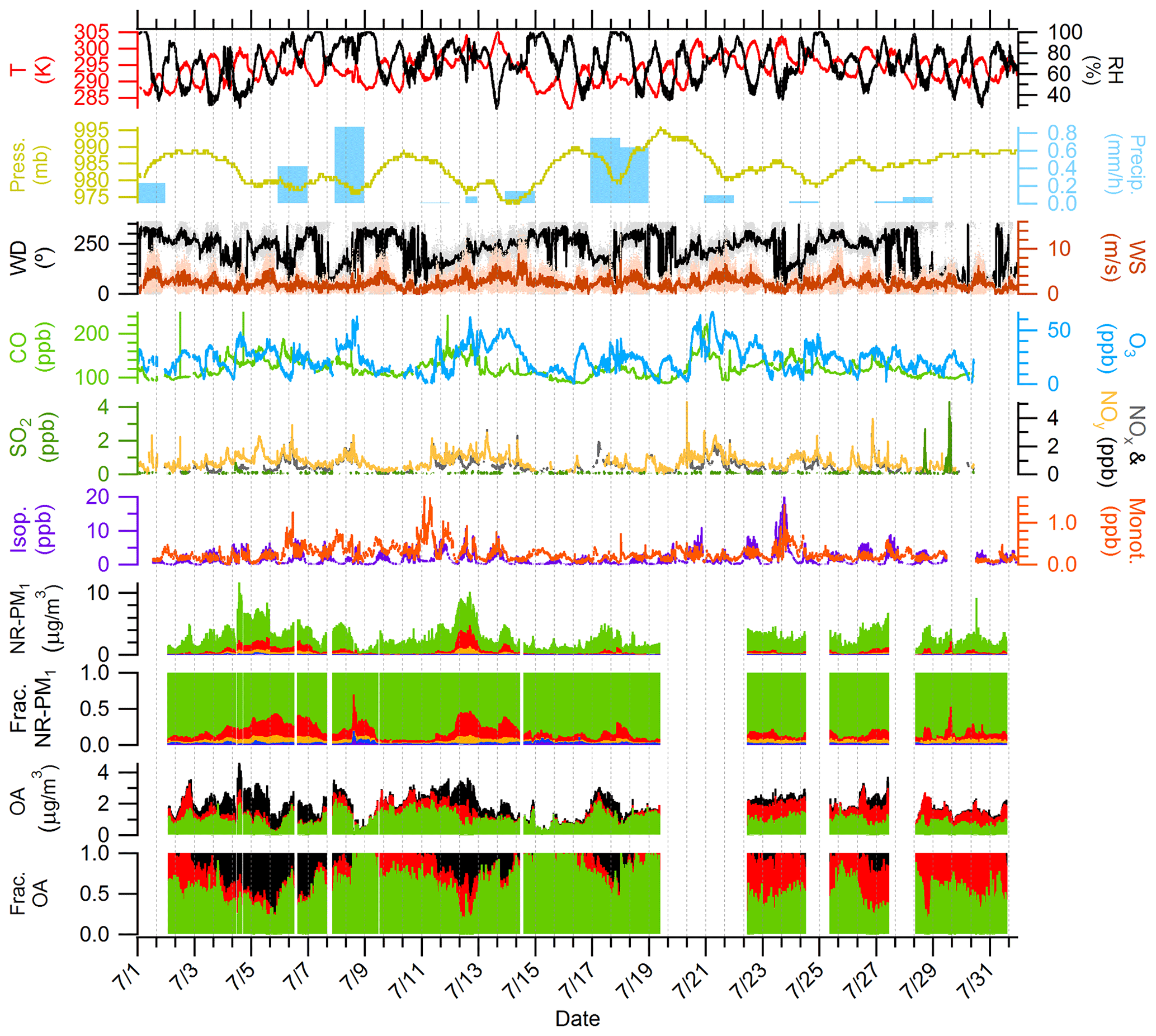
Figure 1 Overview of time series of the following from top to bottom: temperature (T) and RH; pressure (Press.) and precipitation (Precip.); wind direction (WD) and wind speed (WS); CO and O₃; SO₂, NO_x, and NO_y; isoprene (Isop.) and total monoterpenes (Monot.); particulate OA (green), NO₃ (blue), SO₄ (red), NH₄ (orange), and Chl (purple); fraction of species to total NR-PM₁; OA factors derived from PMF; and fractional contribution of OA factors to total OA. OA factors are colored as follows: MO-OOA (black), IEPOX-OA (red), and 91Fac (green). Precipitation data are provided from the NADP site in Cheboygan County, MI. Trace gas data (CO, O₃, SO₂, NO_x, and NO_y) are measured from the 6 m inlet on the MAQL. Meteorological data (T, RH, Press., WD, and WS) and VOC data (Isop. and Monot.) are measured from the 34 m inlet on the PROPHET tower. The OA time series include data from both heights (6 and 30 m), with the sampling switched at 10 min intervals. The date format is month/day.

Diurnal plots for OA, SO₄, NH₄, NO₃, O : C, and H : C are shown in Fig. S25. The diurnal profiles of OA, SO₄, and NH₄ are all relatively flat and do not have a clear diurnal trend. The lack of clear diurnal variations for SO₄ is consistent with regional transport as the source of SO₄ during this campaign. The diurnal variations in NO₃ show increases in the morning, with a maximum around approximately 10:00 local time, and lower concentrations in the afternoon.

Using the backward-trajectory clustering results described in Sect. 3.1, mean values of NR-PM₁, NR-PM₁ species, OA elemental ratios, meteorological parameters, and trace gases for the entire campaign and for northerly and southerly backward-trajectory clusters are shown in Table 1. Overall, relative to northerly air masses, southerly air masses were found to be warmer (∼2 ^∘C); more humid (∼5 %); and associated with higher concentrations of NO_x, NO_y, O₃, and benzene. Furthermore, on average, southerly air masses had higher concentrations of NR-PM₁, OA, SO₄, NH₄, and NO₃. Higher levels of OA oxidation (8 % difference) based on O : C are also observed during periods of southerly flow (O : C is 0.69 versus 0.75 for northerly versus southerly flow, respectively). An additional metric of oxidation, the oxidation state of carbon (OSc), indicates that the degree of oxidation is higher during periods of southerly flow (OSc is −0.12 versus 0.06 for northerly versus southerly flow, respectively, where OSc = $\mathrm{2}\cdot \mathrm{O}:\mathrm{C}-\mathrm{H}:\mathrm{C}$) (Kroll et al., 2011). The factor-of-5 difference between northerly and southerly SO₄ is consistent with the increased influence of SO₂ point sources from electric-generating units south of the site in Ohio, Indiana, and Illinois. Overall, these observations demonstrate that anthropogenic influence from southerly flow directly affects NR-PM₁ mass concentrations, NR-PM₁ composition, the degree of OA oxidation, and trace gas mixing ratios at this site. Results are in agreement with VanReken et al. (2015), where southerly air masses or those “anthropogenically impacted” were found to contain higher aerosol loadings (in terms of aerosol volume, particle number, and median particle diameter) and hygroscopicity, along with increased trace gas abundances, as compared to northerly air masses or clean regimes.

Oxygen-containing ion families (C_xH_yO${}_{z>\mathrm{1}}^{+}$) represent over 50 % of the campaign-averaged OA high-resolution mass spectrum, and this high degree of oxygenation is reflected in an average O : C ratio of 0.71 ± 0.08 and an average H : C ratio of 1.49 ± 0.06. A distinct peak at $m/z$ 44 in the average mass spectrum accounts for 14.1 % of the total OA. The peak at $m/z$ 44 is mainly composed of the CO${}_{\mathrm{2}}^{+}$ ion (96.0 % of $m/z$ 44). The ratio of $m/z$ 44 to the total signal in the organic mass spectrum (f₄₄), a surrogate for O : C and an indicator for photochemical aging, in this study is 0.14. Together with the average O : C ratio (0.71) observed in this study, these values are consistent with OOA observed across AMS datasets (Jimenez et al., 2009; Ng et al., 2010). Other prominent ions in the campaign-averaged high-resolution mass spectrum include $m/z$ 55, 82, and 91. Fragments at $m/z$ 55 represent 2.4 % of the total OA and are representative of both oxygenated and hydrocarbon fragments, such as C₃H₃O⁺ (50.2 % of $m/z$ 55) and C₄H${}_{\mathrm{7}}^{+}$ (42.9 % of $m/z$ 55). The possible OA sources leading to increased signal at $m/z$ 82 (0.46 % of total OA) and 91 (0.62 % of total OA) will be discussed in the following section. Figure S25 shows the diurnal variations in O : C and H : C, indicating relatively stable diurnal cycles. Increases in H : C are observed starting at 09:00 before reaching a maximum at midday (13:00) followed by a slow decrease between the hours of 13:00 and 20:00, while an opposite pattern is observed for mean values of O : C.

Table 1 Campaign-averaged values (± 1 standard deviation from the mean) of mass concentrations of NR-PM₁, VOC and trace gas mixing ratios, and meteorological parameters, as well as hourly averaged values associated with northerly and southerly backward-trajectory clusters. Northerly and southerly air masses are defined in Sect. 3.1 using a cluster analysis of HYSPLIT 2 d backward trajectories.

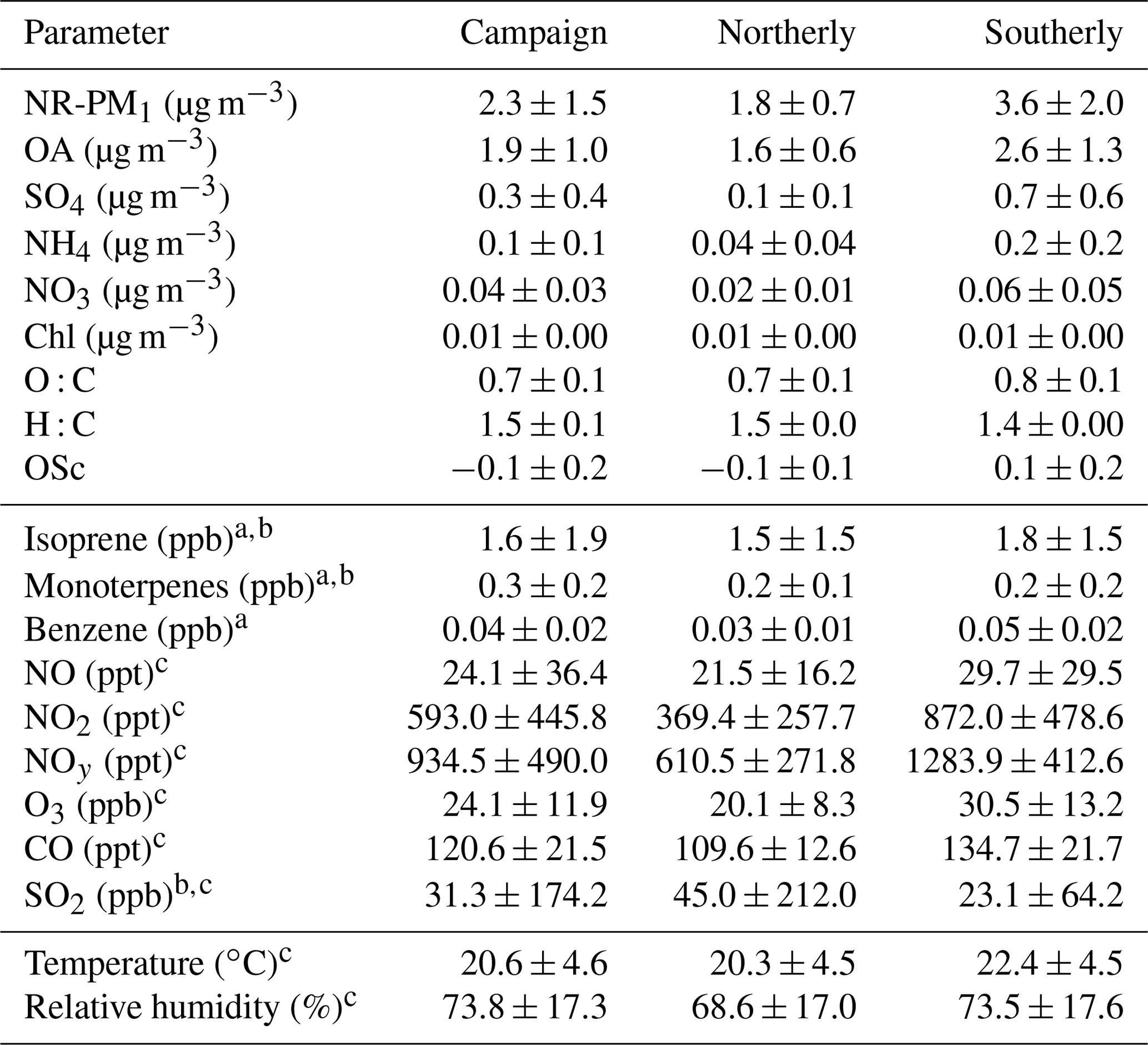
^a VOC measurements using the University of Minnesota's PTR-QiToF instrument from the 34 m inlet on the PROPHET tower. ^b Table entries where the differences between the northerly and southerly backward trajectories mean values are not statistically significant (p<0.01) using a two-sample t test. ^c Trace gas and meteorological parameters measured from on board the MAQL.

3.3 Organic aerosol source apportionment

A three-factor solution is obtained for both the above-canopy inlet at 30 m above the UMBS forest floor (A-MO-OOA, A-IEPOX-OA, A-91Fac) and the below-canopy inlet at 6 m within the UMBS canopy (B-MO-OOA, B-IEPOX-OA, and B-91Fac). 91Fac represents OA with enhanced signal at $m/z$ 91 in the mass spectrum. The addition of more factors to the PMF solution beyond three factors resulted in less physically meaningful and interpretable factors. Thus, the three-factor solution is considered the optimal solution for the above- and below-canopy OA datasets. In this study, SEED = 0 was chosen for both PMF solutions as there was minimal variation in $Q/Q_{\exp }$ across the 50 seeds. Solutions at FPEAK = 0 were chosen because solutions at other FPEAK values did not present improved correlations between factors and reference mass spectra.

Time series of mass concentrations and time series of fractional contributions to total OA are shown in Fig. 1. The O : C ratio of each of the OA factors are as follows: 0.65 (IEPOX-OA), 0.71 (91Fac), and 0.89–0.90 (MO-OOA), all of which indicate the high degree of oxygenation in each of the factors. For the above-canopy PMF solution, 91Fac makes the largest contribution to the total OA (43.8 %), followed by IEPOX-OA (32.8 %) and MO-OOA (23.4 %). For the below-canopy PMF solution, 91Fac also makes the largest contribution to the total OA (42.5 %), followed by IEPOX-OA (34.0 %) and MO-OOA (23.5 %). Details on the chemical composition, mass spectral characteristics, and diurnal profiles of each factor are discussed further in the Supplement.

Hourly averages of the above-canopy OA factors are paired with hourly 2 d backward trajectories for WPSCF analysis. Results from WPSCF analysis using above-canopy OA data (Fig. 2) indicate that A-MO-OOA predominantly originates from southerly air masses, as supported by external measurement data such as of benzene, OVOCs, carbonyls, and SO₄. Air masses that originate from the south pass over the large urban centers of Chicago, Milwaukee, and Detroit. This further supports the aged, transported nature and anthropogenic influences of the observed A-MO-OOA at this site. In contrast, no strong indication of a distinct source region is observed for 91Fac. This could suggest a more localized source of 91Fac in relation to the site. Combining these WPSCF results with correlations of 91Fac with VOC masses corresponding to monoterpene oxidation suggests that 91Fac is sourced from local, biogenic, monoterpene-oxidation-related chemistry (Xu et al., 2018). Finally, WPSCF results for A-IEPOX-OA indicate that this OA factor coincides with more northerly airflow with some contributions from northwesterly flow. These northerly source regions driving A-IEPOX-OA correspond to more rural, less anthropogenically influenced locations in Canada. Interestingly, an instance of high WPSCF values for A-IEPOX-OA and A-MO-OOA can be traced back to areas near the southeastern tip of Missouri and western Tennessee, implying long-range transport of these OA factors. Backward trajectories associated with this instance of high WPSCF values for IEPOX-OA pass over areas in the high-isoprene-emitting region in the Ozarks of southern Missouri, which is commonly referred to as the “isoprene volcano” (Carlton and Baker, 2011; Wiedinmyer et al., 2005). The median mass concentrations of above-canopy OA factors used as the criterion values for the WPSCF method were A-MO-OOA, 0.31 µg m⁻³; A-91Fac, 0.68 µg m⁻³; and A-IEPOX-OA, 0.58 µg m⁻³. Overall, WPSCF analysis indicates that transport from southerly flow (A-MO-OOA), local sources (A-91Fac), and transport from northerly flow (A-IEPOX-OA) are related to the OA factors observed at this site.

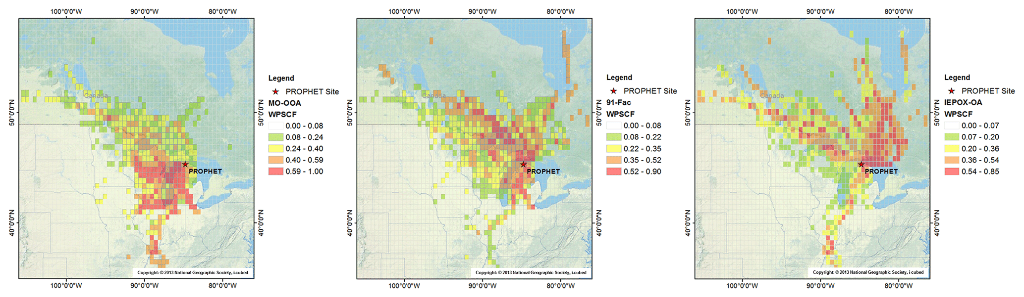
Figure 2 WPSCF backward-trajectory analysis maps for the following hourly averaged OA factors from left to right: above-canopy MO-OOA, above-canopy 91Fac and above-canopy IEPOX-OA. The geographical location of the PROPHET site is represented by a red star. WPSCF analysis is performed using HYSPLIT 2 d backward trajectories, a grid cell size of 0.5^∘ by 0.5^∘, and the geographical domain of the extents of the 2 d backward trajectories. Median mass concentrations of above-canopy OA factors (A-MO-OOA: 0.31 µg m⁻³, A-91Fac: 0.68 µg m⁻³, and A-IEPOX-OA: 0.58 µg m⁻³) are used as the criterion WPSCF values. Color scales correspond to probability of source regions for each respective OA factor, and it should be noted that the range and gradation of the color scale changes between each plot. Map was generated using ArcMap10.1 using the 2013 National Geographic Society, i-cubed basemap. Copyright: © 2013 National Geographic Society, i-cubed.

Overall, PMF analysis for both sampling inlets at the site indicates that the OA is a combination of MO-OOA, 91Fac, and IEPOX-OA. The dominant OA factor is 91Fac, and during periods of southerly flow MO-OOA contributes relatively more (the time series of the fractional contributions to total OA shown from both inlets is shown in Fig. 1 and is also shown separately for each inlet in Figs. S13 and S22). On average, source apportionment results indicate that the OA at both inlets generally had similar average fractional OA contributions and degrees of oxidation. Diurnal profiles for above- and below-canopy OA are shown in Fig. 3 and indicate that diurnal profiles and variations are similar between the two inlets for each OA factor. It is worth noting the diurnal pattern of the IEPOX-OA factor, likely indicating a relatively small influence of local isoprene emissions.

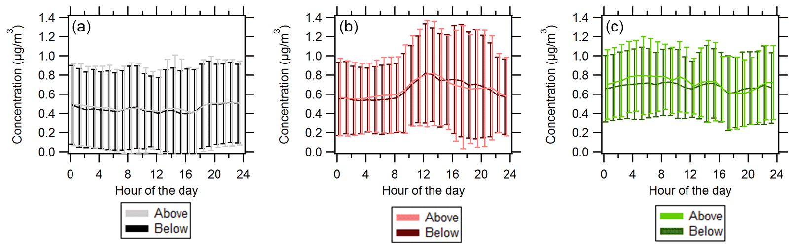
Figure 3 Diurnal profiles of (a) MO-OOA, (b) IEPOX-OA, and (c) 91Fac where solid lines represent average values and whiskers represent 1 standard deviation from the mean. Darker colors represent below-canopy OA (B-MO-OOA, B-IEPOX-OA, B-91Fac) while lighter colors represent above-canopy OA (A-MO-OOA, A-IEPOX-OA, A-91Fac). Data for below-canopy OA factors have been offset by 15 min simply to aid plot interpretation.

3.4 Vertical characterization of above- and below-canopy NR-PM₁ and OA factors

3.4.1 Similarity between above- and below-canopy environments

Mean values of NR-PM₁, NR-PM₁ species, OA elemental ratios, meteorological parameters, VOCs, and trace gases from the above- and below-canopy inlets are summarized in Table 2. Each of the mean values for the parameters listed in Table 2 are within 1 standard deviation of each other for the below- and above-canopy sampling heights. However, results from Wilcoxon rank-sum tests indicate that the medians for a majority of the above- and below-canopy parameters are significantly different (p=0.05). To provide a comparison of the two inlets on the same timescale, scatterplots of 30 min averaged values are shown in Fig. 4 for OA factors, total OA, SO₄, and O : C. For reference, a 1 : 1 line is shown on each scatterplot. Values falling within 1 standard deviation are similar between above and below the canopy, while values deviating farther from the 1 : 1 line indicate values in which the above- or below-canopy environment had differing concentrations. Figure 4 illustrates that mass concentrations of OA factors, total OA, and SO₄ were similar over a majority of the campaign and suggests that the above- and below-canopy environments were generally coupled from a PM perspective. It also appears that total OA, MO-OOA, IEPOX-OA, and 91Fac show increases above the canopy relative to below the canopy at the highest end of the range of the measurements.

Results from a recent study from the PROPHET–AMOS 2016 campaign by Millet et al. (2018) indicate that flux of isoprene and monoterpenes at the canopy–atmosphere boundary represents over half of the net carbon flux while OVOCs constitute a majority of the species with detectable VOC fluxes. Overall, the authors report that the observed and modeled net carbon flux during the campaign was upward (canopy emission) during the campaign in 2016. Additionally, in-canopy gradients of directly emitted BVOCs, such as isoprene and monoterpenes, indicate patterns that are consistent with their respective temperature, light, and physical emission dependencies (higher concentrations in the canopy for isoprene and higher in the lower canopy for monoterpenes). On the other hand, in-canopy gradients of secondary products from BVOC oxidation, such as acetic acid and glycolaldehyde, indicate patterns consistent with net nighttime uptake and a weak peak concentration near the mid-canopy. Correlation analysis of these secondary oxidation products and HCOOH indicates that HCOOH likely originates from a secondary source in this environment (Alwe et al., 2019). In the present study, the overall homogeneity in OA factors implies that, despite vertical gradients in trace gases and BVOCs from primary emission and secondary production, turbulent mixing of aerosols between the forest canopy and the atmosphere is efficient.

Table 2 Campaign-averaged values (± 1 standard deviation) of mass concentrations of NR-PM₁, VOC, and trace gas mixing ratios and meteorological parameters above and below the canopy.

^a Summary statistics for NR-PM₁ measurements were calculated using 5 min averaged data, VOC measurements using 1 min averaged data (University of Minnesota's PTR-QiToF 5 m inlet and 34 m inlet), NO_x above-canopy measurements using 5 min averaged data (University of Toronto), NO_x and O₃ below-canopy measurements using 5 min averaged data (MAQL), and O₃ using 1 min averaged data (CU Boulder's 27 m inlet on the AmeriFlux Tower). ^b Percent of data below detection limit for NR-PM₁ – NH₄ (4 %/4 %) and Chl (59 %/63 %) – and for VOCs – isoprene (30 %/30 %), monoterpenes (56 %/36 %), benzene (100 %/100 %), and NO (37 %/22 %) – where percentages are shown for above-/below-canopy data. Unless otherwise stated, the percentage below the detection limit for all other parameters is 0 %. ^c Table entries where the null hypothesis (“equal medians”) between the above- and below-canopy data cannot be rejected and was not statistically significant (p>0.05) using a two-sided, non-parametric Wilcoxon rank-sum test. All other table entries indicate that the null hypothesis (equal medians) can be rejected at a statistically significant level (p<0.05).

Furthermore, this similarity between the above- and below-canopy environments suggests that the chemical timescales of SOA formation processes likely are long relative to residence times due to turbulent mixing (Foken et al., 2012), assuming relatively constant background levels. Ultimately, the observed similarity agrees with previous modeling work that predicts similar SOA mass loadings at these two heights (Ashworth et al., 2015; Schulze et al., 2017). The results shown in the present work also are in agreement with measurements at the site in 2009, showing that aerosol gradients on the PROPHET tower “existed at times between the above-canopy (31.4 m) and understory environments (5 m)” but that the understory conditions were generally similar to that of the above-canopy conditions (VanReken et al., 2015). The vertical similarity in NR-PM₁ is also in agreement with findings in the Amazon forest, where a balance between upward and downward fine particle fluxes was found (Rizzo et al., 2010) and in a southeast Asian rainforest, where PM₁ did not show significant variations with height during the daytime (Whitehead et al., 2010).

Figure 4 Scatterplots of above-canopy (A) and below-canopy (B) hourly averaged values for (a, b) SO₄ and total OA, (c, d) MO-OOA and 91Fac, and (e, f) IEPOX-OA and campaign O : C. The three-way valve switched between the two inlets at 10 min intervals, so 30 min averaged mass concentrations allow for a comparison of both inlets on the same time basis. Above-canopy values are plotted on the y axis of each plot, and below-canopy values are plotted on the x axis of each plot. Averages are shown with squares; whiskers represent 1 standard deviation from the mean. For reference, a 1 : 1 line is shown with each plot. Outliers on the O : C plot corresponding to periods of precipitation were removed.

3.4.2 Episodes of vertical differences in NR-PM₁

Episodes of vertical differences in NR-PM₁ between the two inlets were observed, and four such episodes are described here: Episode 1 (Period: 3 July 2016 19:30 to 5 July 2016 15:00 LT), Episode 2 (11 July 15:00 to 12 July 23:00 LT), Episode 3 (16 July 2016 21:30 to 19 July 2016 08:30 LT), and Episode 4 (26 July 2016 08:30 to 31 July 2016 13:30 LT). Episodes were defined as sustained periods in which a vertical difference in OA or SO₄ was greater than or equal to concentrations representing ≥25 % of the campaign-averaged OA or SO₄. The “vertical difference”, symbolized as Δ in Fig. 5, is defined as the difference between above- and below-canopy values, where the positive convention indicates larger concentrations above the canopy. Episodes 1, 3, and 4 indicate increased above-canopy OA concentrations, while Episode 2 indicates increased below-canopy SO₄ concentrations. Episodes with higher above-canopy NR-PM₁ ranged up to ∼ 1.0 µg m⁻³ higher in OA and ∼ 0.5 µg m⁻³ higher in SO₄ relative to equivalent above/below mass (Δ=0). Figure 5 shows time series of vertical differences in OA factors and SO₄ and estimates of friction velocity (u^*) at five different heights (not equal to those for the VOC measurements) on the PROPHET tower over the campaign. Calculated from three-dimensional wind velocity data, u^* is a function of the shear stress at the surface and is used in this study as a metric of in-canopy mixing (Eq. 5).

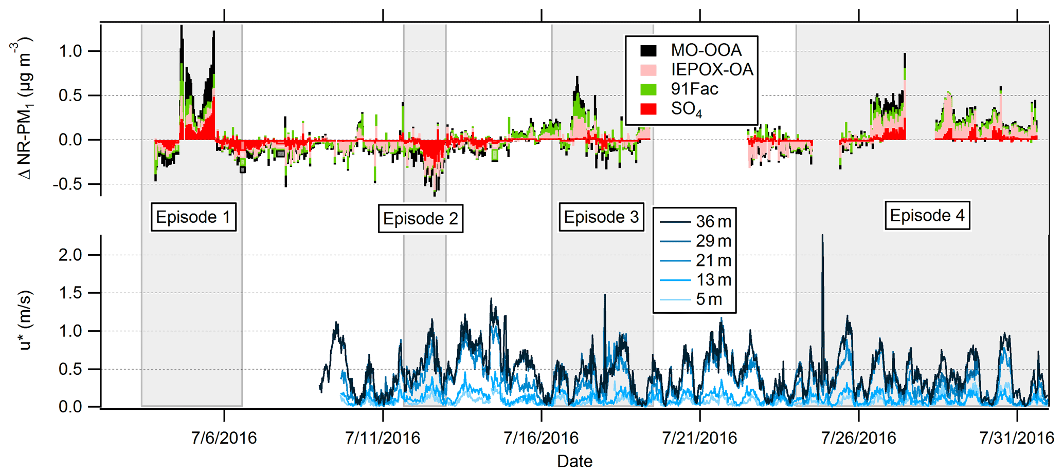
Figure 5 Time series of (top) observed NR-PM₁ vertical differences between above- and below-canopy inlets and (bottom) friction velocity (u^*) in m s⁻¹ at five different heights on the PROPHET tower. Vertical differences are defined as Δ species, where Δ refers to the above-canopy minus the below-canopy mass concentration. Note that the elevations for u^* are slightly different than those for trace gas sampling. The date format is month/day/year.

The sums of the delta values for each OA factor (∑ΔOA factors) for the episodes are shown in Fig. 6 with corresponding observations of u^* and vertical differences in SO₄ and O₃. Figure 6 shows that vertical differences in OA correlate with vertical differences in SO₄ for Episodes 1 and 4, while ∑ΔOA factors during Episode 3 coincides with higher above-canopy O₃ concentrations. Correlations between chemical species for Episode 2 are weaker. Correlation coefficients (r) for each episode are 0.69 (Episode 1 ∑ΔOA factors–sulfate), −0.44 (Episode 2 sulfate–u^*), 0.34 (Episode 3 ∑ΔOA factors–ozone), and 0.59 (Episode 4 ∑ΔOA factors–sulfate). These episodes have different OA factor compositions: MO-OOA contributes a larger percentage during Episodes 1 and 2, 91Fac contributes roughly half in Episode 3, and IEPOX-OA contributes more than half of the total OA vertical difference in Episode 4.

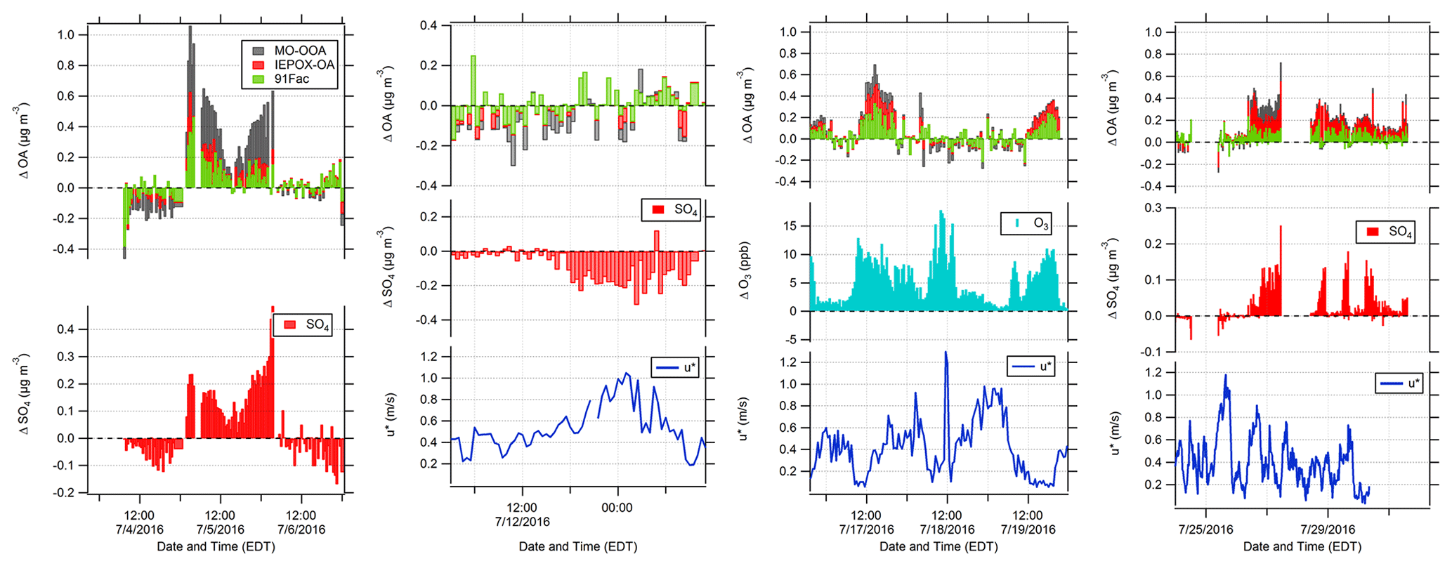
Figure 6 Time series of observed NR-PM₁ vertical-difference episodes: (from left to right) Episode 1, Episode 2, Episode 3, and Episode 4. Data shown for Episode 1, Episode 2, and Episode 4 include vertical differences in 30 min averaged above- and below-canopy SO₄, while data shown for Episode 3 show vertical differences in 30 min averaged above- and below-canopy O₃. The O₃ data were measured from the AmeriFlux Tower at 6 and 27 m and were provided courtesy of CU Boulder. Friction velocity measurements at 29 m on the PROPHET tower are also provided for Episodes 2–4. The date format is month/day/year.

3.5 The role of mixing and particulate SO₄ in vertical differences in OA

The diurnal profiles of vertical-difference episodes for total OA, SO₄, and OA factors in 2016 indicate there is no clear diurnal pattern observed for any of these species (Fig. S26). Maximum vertical differences for SO₄, total OA, and MO-OOA are observed around 15:00. For total OA, a gradual increase occurs at 09:00 before reaching a maximum vertical difference at 15:00, suggesting that the episodes of higher above-canopy NR-PM₁ begin shortly after the most commonly observed hours of canopy uncoupling from the site in 2009. The initiation of these events may also be attributed to venting of the nocturnal boundary layer as it breaks up in the morning hours, as observed for events of upward particle number fluxes by Whitehead et al. (2010).

To assess the agreement between the occurrence of episodes and micrometeorological measurements of in-canopy mixing, episode-specific data for Episodes 2–4 are shown in Fig. 6. During Episode 1, u^* data are available only at 36 m, so no friction velocity data are shown, preventing a full analysis similar to those performed for the other three episodes. However, based on similarity in sulfate enhancements, it can be assumed that Episode 1 is somewhat similar to Episode 4.

During Episode 2, based on the backward-trajectory cluster analysis shown in Table 1 and the WPSCF results, regional transport is the likely source of the PM, including the enhancements below the canopy. Prior to this episode, SO₄ and MO-OOA are uniform from below to above the canopy. The below-canopy enhancement then reaches up to 0.3 µg m⁻³ of SO₄. Downmixing of clean air from aloft could lead to lower concentrations above the canopy, meaning that the observed difference would be caused by decreasing above-canopy concentrations, not increasing below-canopy concentrations. However, below-canopy concentrations are observed to increase while above-canopy concentrations decrease. Without a local, below-canopy source, this indicates that pollutants from above the canopy are mixed into the below-canopy region at a rate faster than they are lost to deposition. Regional pollutants, advected to the site above the boundary layer, can be mixed down to the surface with daytime boundary layer growth, as has been found in previous aircraft campaigns (Berkowitz et al., 1998; Thornberry et al., 2001). Downward transport of air masses from the surrounding region has also been hypothesized to contribute to higher ratios of organic nitrogen to organic carbon in water-soluble aerosols within a forest canopy relative to its forest floor (Miyazaki et al., 2014).

During Episodes 3 and 4, periods of above-canopy enhancement in OA factors coincide with relatively lower u^* ($u^{*}<\mathrm{0.2}$ m s⁻¹ during Episode 3 and $u^{*}<\mathrm{0.6}$ m s⁻¹ during Episode 4, with the average u^* considering all heights over the duration of the episode), with lower friction velocities and greater above-canopy enhancement in Episode 3. In the case of Episode 3, lower in-canopy mixing, mostly occurring during nighttime, agrees well with periods of higher above-canopy OA factor and O₃ concentrations. In this case, both IEPOX-OA and 91Fac contribute to the OA enhancement, likely due to strong photochemistry both locally and during transport (as indicated by increased O₃). Episode 4 is the longest-duration episode; however, the agreement between low-mixing conditions and above-canopy PM enhancements is more variable during this case. Similarly to Episode 3, the lowest values of friction velocity occur during the nighttime or early morning. Despite the temporal misalignment of ΔOA and low u^*, it should be noted that friction velocities lower than the campaign average (∼ 0.4 m s⁻¹) are observed during the latter periods of Episode 4 (28–30 July), which is consistent with the low-mixing hypothesis presented for Episode 3. Therefore, it appears that stagnant conditions above the canopy created an environment where canopy exchange became limited and air masses did not fully penetrate into the canopy; aerosol deposition below the canopy potentially enhanced the positive delta values. This scenario could also promote in-canopy OA accumulation, but this does not appear to have occurred, implying that other factors contributed to these vertical differences. Instead, it appears that increased sulfate loading was associated with this transport and that this increased sulfate above the canopy led to enhancements above the canopy, particularly of IEPOX-OA relative to 91Fac, as shown in Fig. 6. This could also be related to associated changes in aerosol liquid water.

The probability distributions of ΔSO₄ and ΔO₃ between episodes and the average for the entire PROPHET campaign are compared in Fig. S27. The cumulative distribution function (CDF) for ΔSO₄ indicates that Episodes 1 and 4 had higher probabilities of positive ΔSO₄ (denoting higher above-canopy concentrations), while Episode 2 had higher probabilities of negative ΔSO₄ (denoting higher below-canopy concentrations). The episode-specific CDFs for Episodes 1 and 2 are also different from the total campaign CDF, implying that the vertical differences observed were distinct events. The average O₃ difference between the 6 and 27 m inlets on the AmeriFlux tower throughout the campaign indicated that O₃ was on average 5 ppb greater at the 27 m inlet, with the difference reaching as high as 34 ppb on 6 and 20 July. The probability distribution of vertical O₃ differences observed during Episode 3 is markedly different than those observed during Episode 1, Episode 4, and the remainder of the campaign. This indicates that O₃ had a larger probability of being between 0–10 ppb higher above the canopy during this episode compared to during the rest of the campaign.

Based on Episode 1 and Episode 4, one of several potential driving factors of vertical differences for OA is a vertical difference in particulate SO₄. Figure 7 indicates the vertical differences in OA and SO₄ relative to their respective above-canopy concentrations. This metric is defined as the percent PM difference, where PM is the given PM constituent and is equal to the ΔPM constituent divided by the above-canopy PM concentration. Data that fall in the upper right and bottom left quadrants correspond to higher above-canopy and higher below-canopy concentrations, respectively. The vertical difference above or below the canopy can be up to approximately 35 % of the total available SO₄ or OA at the site. Figure 7 indicates that there is a strong linear relationship between the percent SO₄ difference and percent OA difference during the campaign, even outside of the episodes defined here.

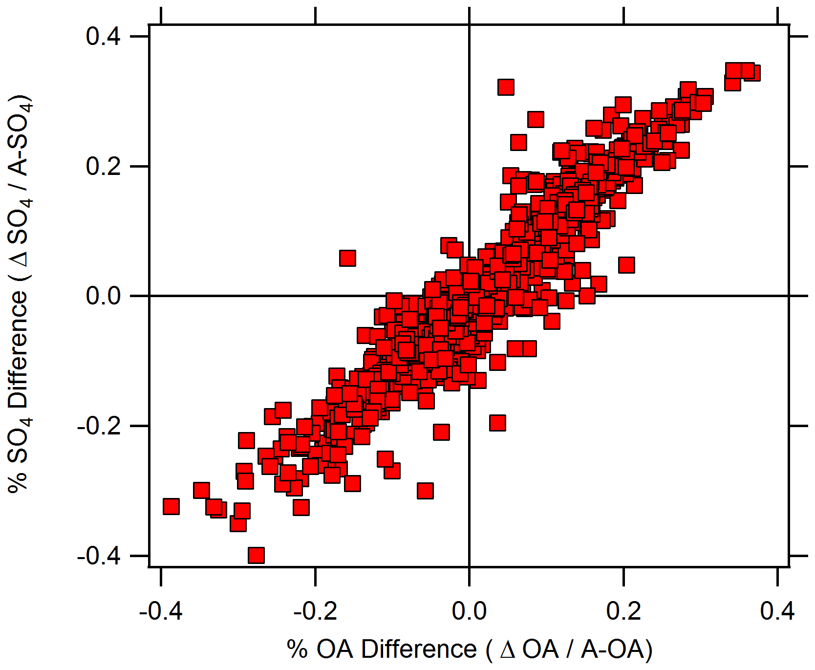
Figure 7 Scatterplot of percent difference in SO₄ (y axis) and OA (x axis) for the entire campaign. The percent difference is calculated as Δ species $/$ above-canopy species concentration and is representative of the normalized Δ species concentration.

The concurrent features of vertical differences in OA factors and SO₄ observed in Episodes 1, 2, and 4 and OA factors and O₃ in Episode 3 suggest that long-range regional transport (enhanced MO-OOA, SO₄, and/or O₃) is a key first step in causing these differences. Local through-canopy mixing then determines whether the enhancement is above (Episodes 1, 3, and 4) or below (Episode 2) the canopy. The transported material can then impact local chemistry. Increased SO₄ likely increases aerosol hygroscopicity, resulting in increased ALW, which could result in increased partitioning of semi-volatile organics to the condensed phase (i.e., IEPOX-OA) (Budisulistiorini et al., 2017; El-Sayed et al., 2018; Marais et al., 2016). Pre-existing OA (i.e., MO-OOA) transported with SO₄ aerosol could also play a role in the partitioning of OA above the canopy during these episodes. Vertical gradients in O₃ coinciding with Episode 3 (higher O₃ above) could initiate relatively local formation of extremely low volatility compounds, which are first-generation oxidation products of α-pinene and O₃ (Jokinen et al., 2015). Based on the WPSCF and backward-trajectory clustering results, cooler, northerly air masses associated with IEPOX-OA could also promote partitioning of semi-volatile organics to the particle phase. It is important to note that it is difficult to conclude what the exact chemical mechanisms influencing these events are due to their low mass loadings and episodic nature and the consistently higher above-canopy O₃ concentrations during the campaign.

Understanding these events is important because uncoupled forest–canopy conditions have been observed in a number of locations (Foken et al., 2012; Kruijt et al., 2000; Whitehead et al., 2010) and could indicate differences between above-canopy and surface level PM. One-dimensional modeling has revealed that the timescales of turbulent transport inside a forest canopy can be much shorter (minutes) than the timescale of aerosol dynamics and deposition (hours) (Rannik et al., 2016), but this evaluation suggests that advective episodes can cause vertical gradients that are not locally driven. Above-canopy OA and particle fluxes have been observed in other studies (Farmer et al., 2013; Pryor et al., 2007), suggesting the need for careful evaluation of whether differences are driven by local chemistry, long-range transport, or a combination thereof.

3.6 Particle dry deposition model

To investigate broadly the effects of canopy mixing on particle deposition in a forest canopy, a particle dry deposition model is used. Note that we are not applying this through the canopy but to illustrate the relationship between deposition and u^*. The resistance model for particle dry deposition assumes that the deposition process is controlled by three resistances in series: aerodynamic, quasi-laminar, and canopy resistance (Seinfeld and Pandis, 2006). Details on the particle dry deposition model are included in the Supplement. Conditions and parameters representative of the land-use category, season, and forest canopy present at the PROPHET site are used as model inputs.

Figure 8 displays model results for deposition velocity as a function of the particle diameter under stable atmospheric conditions. For illustration, test cases are shown for u^* values for low in-canopy mixing ($u^{*}=\mathrm{0.1}$ m s⁻¹) and high in-canopy mixing ($u^{*}=\mathrm{0.8}$ m s⁻¹). Values of u^* were chosen based on the range of u^* values observed during the campaign at 29 m on the PROPHET tower. For the submicron particle diameter range (0.1 to 1 µm), a characteristic minimum in deposition velocity is observed for both test cases at a 1 µm diameter. Deposition modeling indicates that higher deposition velocities are achieved in the test case for high in-canopy mixing, implying that there is less canopy transport resistance to the surface and more deposition in the canopy. This corresponds to Episode 2.

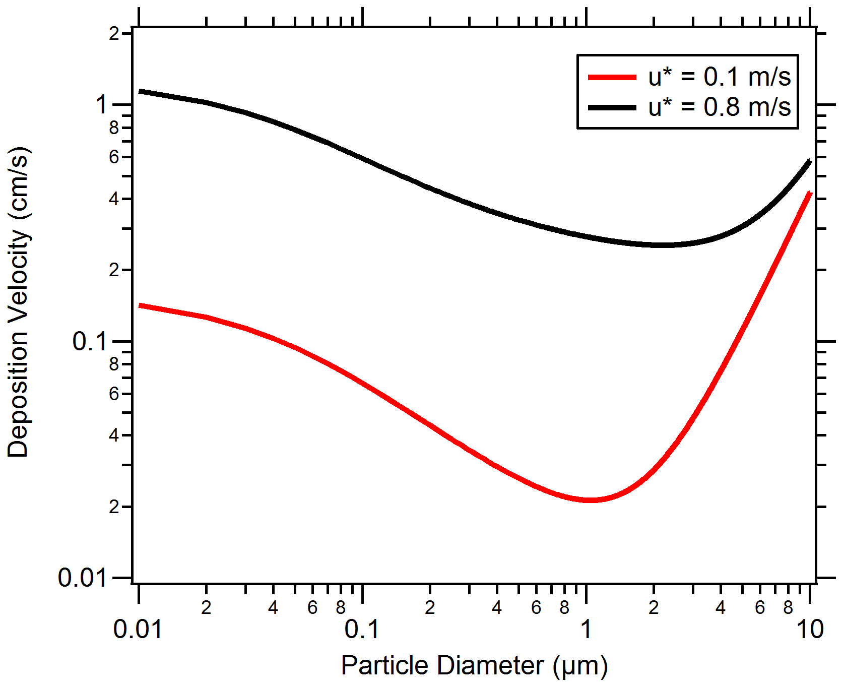
Figure 8 Particle dry deposition velocity resistance model results plotted by particle diameter and friction velocity. Two test cases of low and high friction velocity, representative of data collected at the PROPHET site, are plotted in solid red and black lines, respectively. Land-use conditions and seasonal parameters similar to those of the PROPHET campaign were used as inputs to the particle dry deposition model. Additional model parameters are provided in the Supplement.

Deposition modeling also indicates relatively lower deposition velocities for the low-mixing-condition test case, which suggests that particles aloft are transported less efficiently into the forest (similarly to the conditions present for Episodes 3 and 4). A comparison of the deposition resistances (shown in Fig. 9) indicates that aerodynamic and quasi-laminar resistances in the low-mixing test case are an order of magnitude greater than the high-mixing case. The settling removal resistance is the same between both test cases because it is merely a function of the diameter. A greater aerodynamic resistance limits turbulent transport from the above-canopy layer to the surface layer, and greater quasi-laminar layer resistance limits transport to just above the surface by lowering particle impaction. In total, this result emphasizes the importance of in-canopy transport and mixing in governing particle concentrations in forests.

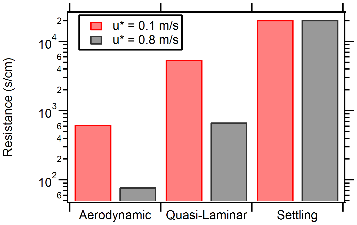
Figure 9 Deposition and particle settling (accounts for the effect of sedimentation) resistance comparison for low and high friction velocities. Resistance comparison assumes a 1 µm particle diameter.

4 Conclusions

In this study, source apportionment of OA using separate PMF analyses on inlets situated above and below a forest canopy resulted in three OA factors at a site in northern Michigan. Similarity in OA composition, concentration, and diurnal profiles was observed between the two inlets, suggesting that turbulent transport efficiently mixes OA across the canopy. However, OA factor vertical differences between the two inlets were observed during four separate episodes. During these episodes, vertical differences were both positive (greater concentrations above the canopy) and negative (greater concentrations below canopy). NR-PM₁ composition among these episodes was unique (Episode 1, MO-OOA dominant; Episode 2, SO₄ dominant; Episode 3, 91Fac dominant; Episode 4, IEPOX-OA dominant). Furthermore, the vertical-difference concentrations can be 35 % of the total available SO₄ or OA at the site. It has also been shown that relative vertical differences in SO₄ and OA are linearly associated, suggesting the role of regional SO₄ in vertical profiles of NR-PM₁ in forested environments.

Using micrometeorological measurements, it has been shown in this work that periods of conditions of low in-canopy mixing can be associated with the timing of vertical-difference episodes where above-canopy concentrations are larger than those below. The opposite scenario is hypothesized to be associated with transport of air from aloft or with accumulation of material below the canopy more rapidly than it is deposited. Either way, these results suggest that canopy mixing impacts particle levels. However, under low-mixing scenarios, it appears that enhancements as defined here depend on both these conditions and the presence of transported O₃ or SO₄ to enhance IEPOX-OA and 91Fac levels.

To the knowledge of the authors, this is one of only a few studies that have assessed vertical profiles in OA factors above and below a forest canopy and the first study to observe episodes of vertical differences in OA factors above and below a forest canopy. This work adds to the existing literature on aerosol chemistry in a forest canopy environment presented by Rizzo et al. (2010) and Whitehead et al. (2010) and to literature on vertical profiles of OA in an urban environment by Öztürk et al. (2013).

To investigate the effects of forest canopies on SOA formation, small-scale models, such as those described in Schulze et al. (2017) and Ashworth et al. (2015), have been developed. The OA data from this work can be used to validate such models and are particularly relevant to these modeling efforts as the models were developed using campaign data from the PROPHET site in 2009. Vertical transport and horizontal advection are both sources of uncertainty in current forest canopy–atmosphere exchange models, which are designed to focus on local processes. Ultimately, the vertical similarity in NR-PM₁ OA composition observed in this study implies that it may be valid to assume that below-canopy OA composition is generally representative of the OA composition in the atmospheric layer directly above the canopy and vice versa. However, this work highlights that advection of regional pollution into forested regions can lead to in-canopy gradients that are not present under purely local conditions.