Hyperfine-resolution mapping of on-road vehicle emissions with comprehensive traffic monitoring and an intelligent transportation system

Urban on-road vehicle emissions affect air quality and human health locally and globally. Given uneven sources, they typically exhibit distinct spatial heterogeneity, varying sharply over short distances (10 m–1 km). However, all-around observational constraints on the emission sources are limited in much of the world. Consequently, traditional emission inventories lack the spatial resolution that can characterize the on-road vehicle emission hotspots. Here we establish a bottom-up approach to reveal a unique pattern of urban on-road vehicle emissions at a spatial resolution 1–3 orders of magnitude higher than current emission inventories. We interconnect all-around traffic monitoring (including traffic fluxes, vehicle-specific categories, and speeds) via an intelligent transportation system (ITS) over Xiaoshan District in the Yangtze River Delta (YRD) region. This enables us to calculate single-vehicle-specific emissions over each fine-scale (10 m–1 km) road segment. Thus, the most hyperfine emission dataset of its type is achieved, and on-road emission hotspots appear. The resulting map shows that the hourly average on-road vehicle emissions of CO, NO_x, HC, and PM_2.5 are 74.01, 40.35, 8.13, and 1.68 kg, respectively. More importantly, widespread and persistent emission hotspots emerged. They are of significantly sharp small-scale variability, up to 8–15 times within individual hotspots, attributable to distinct traffic fluxes, road conditions, and vehicle categories. On this basis, we investigate the effectiveness of routine traffic control strategies on on-road vehicle emission mitigation. Our results have important implications for how the strategies should be designed and optimized. Integrating our traffic-monitoring-based approach with urban air quality measurements, we could address major data gaps between urban air pollutant emissions and concentrations.

1 Introduction

Urban air pollution is a critical risk for premature death globally (Lelieveld et al., 2015; West et al., 2006). A primary reason for this is the rapid growth in vehicle population over decades, which has led to widespread and severe pollution of fine particulate matter (PM_2.5) and ozone (O₃) (Anenberg et al., 2017; He et al., 2020; Huang et al., 2020; Kelly and Zhu, 2016; Tessum et al., 2014; Zhang et al., 2012, 2019). Thus, the budget assessment of on-road vehicle emissions is of great significance for air pollution control, epidemiology, exposure assessment, and environmental equity (Anenberg et al., 2017). However, the gradients of on-road vehicle emissions are not well represented in routine emission inventories. The main concern is that the traffic states (e.g., traffic fluxes, road conditions, and vehicle categories) can vary sharply over short distances (10 m–1 km), particularly in urban zones (Chen et al., 2020; Gately et al., 2017; Liu et al., 2019; Wu et al., 2020; Yu et al., 2020).

Routine inventories of on-road vehicle emissions are established based on macro-scale and retrospective statistics. Consequently, they are temporally static for a historical year or month and spatially coarse ($>\mathrm{1}\times \mathrm{1}$–25×25 km²) (Janssens-Maenhout et al., 2015; Li et al., 2017; Zhang et al., 2013). Earlier studies have applied traffic models to improve the spatiotemporal resolution (Zhang et al., 2016). However, given that the traffic states were assumed, the simulated emissions were prone to deviate from real-world situations, especially from fine-scale gradients. More importantly, the emission hotspots and their anthropogenic drivers are missed.

Recently, significant advances have been made in comprehensive traffic monitoring techniques. They can help increase the spatiotemporal resolution of traffic states. These methods include GPS-instrumented floating cars (e.g., GPS-equipped probe taxis), open-access congestion maps, radio frequency identification, and traffic video records, each of which has distinct advantages and limitations (Gately et al., 2017; Gately and Hutyra, 2017; Jing et al., 2016; Liu et al., 2018; Wen et al., 2020; Wu et al., 2020; Yang et al., 2018b, 2019). The individual GPS-instrumented floating cars allow us to extrapolate regional-scale vehicle activity levels. Yet, they are relatively scarce compared to the whole fleet, unable to characterize the fine-scale gradients (10 m–1 km) as well as emission hotspots. Open-access congestion maps typically originate from navigation software, such as Baidu Maps. Technically, they collect locations of individual mobile phones as real-time traffic information. On this basis, hierarchical traffic congestion indices can be built up and treated as spatiotemporal surrogates of traffic fluxes and speeds. Despite this, the information for individual vehicles, like speed and categories, remains unavailable. A recent study (Deng et al., 2020) utilized the BeiDou Navigation Satellite System to develop a full-sample high-resolution emission inventory but only for trucks.

In contrast, comprehensive traffic monitoring technologies, such as radio frequency identification (Paul et al., 2013) coupled with traffic video records (Song et al., 2019), can offer valuable opportunities to fulfill real-time vehicle-specific traffic information. Nevertheless, only in a few developed regions do these facilities regularly complete full coverage at a vast expense. Despite this, in the United States, daily traffic activities are released annually at the state level rather than at a high spatiotemporal resolution (hourly and 10 m–1 km) (Gately et al., 2013). On the other hand, those facilities are inter-complementary but usually owned and operated by different governmental agencies or private companies separately. Hence, relying on a single agency or company, hyperfine-resolution emission inventories cannot be derived comprehensively.

To this end, it is essential to introduce an intelligent transportation system (ITS) that is capable of interconnecting the independent traffic monitoring and thus offering a complete picture of traffic states (Avila and Mezić, 2020; Yang et al., 2020; Zhang et al., 2018). Hence, this would be a unique opportunity to derive a hyperfine-resolution on-road vehicle emission inventory. However, for most developing regions, especially in populous parts of Asia and Africa, such an integrated system is largely absent.

As one of the most developed regions in the Yangtze River Delta (YRD), Xiaoshan District is confronting severe air pollution, particularly with surface O₃ frequently exceeding air quality standards in summertime (http://www.cnemc.cn/, last access: 2 September 2021). This indicates the significance of mitigating on-road vehicle emissions. Moreover, it is one of the few representatives for which comprehensive traffic monitoring achieves full coverage and has been interconnected via an ITS (named “City Brain”) since 2017 (Fig. 1) (Hua, 2018). This allows us to calculate single-vehicle-specific emissions over each fine-scale (10 m–1 km) road segment. Consequently, we can derive the largest and most hyperfine urban on-road vehicle emission dataset of its type and capture the emission hotspots. Thus, fine-scale gradients (10 m–1 km) and hotspots of on-road vehicle emissions are exposed. Furthermore, the associated drivers, such as traffic congestion, are further investigated. On this basis, we can directly evaluate the potential impacts of precise (e.g., vehicle-type-specific, road-segment-specific, or traffic-flux-specific) emission mitigation strategies. Our results provide new insights into the spatial variability of urban on-road vehicle emissions.

Figure 1 A hyperfine-resolution model framework for on-road vehicle emissions. Traffic monitoring includes radar velocimeters and surveillance cameras. License plates, speed, categories, and traffic fluxes are collected. The speed- and category-dependent emission factors are obtained from the local official vehicle I/M dataset. Road segments are divided into three road classes: highways, arterial roads, and residential streets. An intelligent transportation system (ITS) (named City Brain) is developed to interconnect these input data. An image recognition algorithm is embedded to recognize the category for a certain vehicle. Detailed information is given in Sect. 2.2.

2 Materials and methods

In brief, the objective of this study was to apply a bottom-up model approach to establish a hyperfine-resolution inventory of on-road vehicle emissions over Xiaoshan District in the YRD (Fig. 1). All key input data, including traffic fluxes, vehicle-specific categories, and speeds, were obtained from comprehensive traffic monitoring coupled with an ITS. Besides, vehicle-specific emission factors came from the local official vehicle inspection and maintenance (I/M) dataset, the methodology of which was described in China's National Emission Inventory Guidebook (ICCT, 2020).

2.1 Comprehensive traffic monitoring network

Xiaoshan District is located in the hinterland of the YRD in China (Fig. 2). In 2019, it had a population of over 1.58 million, 18.56 % of the population of New York. Its GDP was close to CNY 200 billion, ranking fifth among districts in China. The total length of the road network was around 2000 km within a limited geographical extent (i.e., 1417.83 km²). Against this background, Xiaoshan District has become an important urban transportation hub in the YRD. Therefore, on-road vehicle emissions were projected to be intensive and play a critical role in affecting fine-scale air quality and exposure equity. Since 2016, routine measures to ease traffic congestion, such as license restrictions during the morning and evening rush hours (from 07:00 to 09:00 and from 16:30 to 18:30 local time) on weekdays (i.e., from Monday to Friday), have been implemented over Xiaoshan District. This will have significantly altered fine-scale spatiotemporal patterns of traffic states (including traffic fluxes, vehicle speeds, and fleet compositions) and thus on-road vehicle emissions, but the impacts remain unclear.

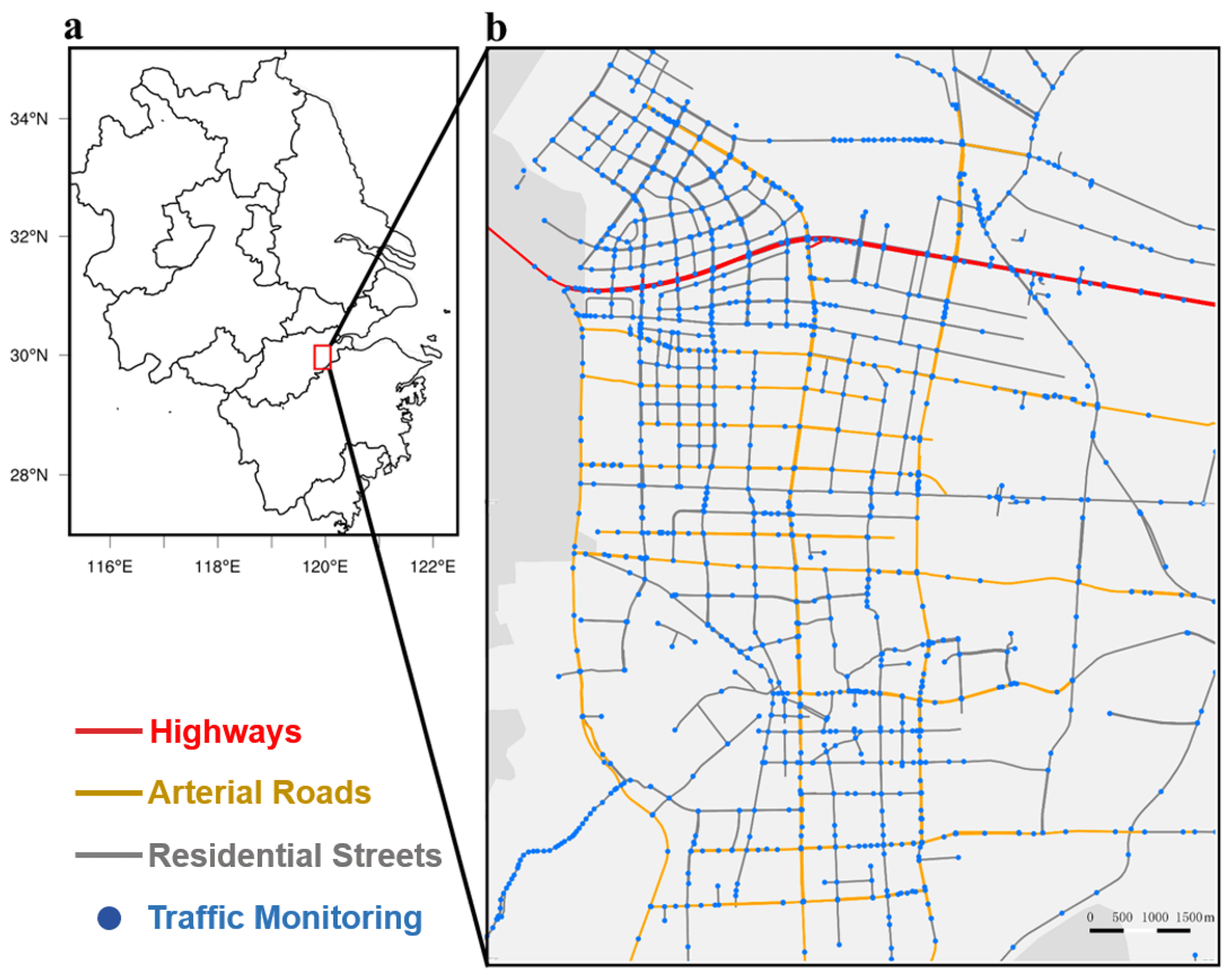
Figure 2 Comprehensive traffic monitoring network in Xiaoshan District. (a) Xiaoshan District (the red rectangle) is located in the hinterland of the YRD in China. (b) Comprehensive traffic monitoring achieves full coverage over Xiaoshan District. Each dot represents a set of comprehensive traffic monitoring platforms that can recognize traffic fluxes, vehicle-specific speed, categories, and license plates. The gaps between two sets, ranging from 10 m to 1 km, determine the spatial resolution of the road and emission map. The entire road network over Xiaoshan District is divided into 1894 road segments. Such road segments are divided into three road classes: highways (red lines), arterial roads (yellow lines), and residential streets (grey lines). Map data © 2021, Gaode Map.

2.2 Hyperfine-resolution bottom-up model framework

A hyperfine-resolution bottom-up model framework was established to calculate primary on-road vehicle emissions, including carbon monoxide (CO), hydrocarbon (HC), nitrogen oxides (NO_x), and PM_2.5. Figure 1 is a flow diagram to illustrate the overall methodology for this framework. The results depended on an ensemble calculation of traffic fluxes, road segments, vehicle-specific speed, categories, and emission factors (Eq. 1) (Wu et al., 2020; Yang et al., 2019; Zhang et al., 2016):

$$\begin{array}{}\text{(1)}& E_{h,j,l}=\sum _t{\text{EF}}_{c,j}\left(v\right)\times {\text{TF}}_{c,h,l}\times L_l.\end{array}$$

$E_{h,j,l}$ is the consequent emission of the pollutant j on the road link l at the hour h, the unit of which is grams per hour (g h⁻¹), while the rest of the variables denote the input data for the model. EF_c,j(v) is the average emission factor of the pollutant j for the vehicle category c at the speed v, the unit of which is grams per kilometer (g km⁻¹); ${\text{TF}}_{c,h,l}$ is the traffic flux of the vehicle category c on the road segment l at the hour h, in units of vehicles per hour (veh h⁻¹); L_l is the length of the road segment l in units of kilometers (km).

The major technical advance in this study was that all these input data were vehicle-specific and obtained from all-around traffic monitoring, introduced and detailed in Sect. 2.3. Detailed road segments are important carriers reflecting traffic states and on-road vehicle emissions. In this study, we divided the entire road network over Xiaoshan District into 1894 road segments. Over the entire district, such road segments were divided into three road classes: highways, arterial roads, and residential streets (Fig. 2). Spatially, each road segment was adaptive to a set of traffic monitoring platforms that can collect comprehensive traffic profiles, including traffic fluxes, vehicle-specific categories, and speeds. Therefore, the all-around traffic monitoring derived the hyperfine-resolution map of road segments and thus $E_{h,j,l}$.

To obtain the key input data for this model, we explored traffic monitoring information that achieved full coverage over Xiaoshan District (Fig. 2). On this basis, vehicle-specific speed and categories were collected. Besides, the vehicle-category-specific emission factors were obtained from the local official I/M dataset. Consequently, an ITS (named City Brain) was developed to simultaneously upload the traffic monitoring information and, more importantly, to establish vehicle-specific links between those parameters. Therein traffic fluxes played a major role in affecting vehicle emissions (Deng et al., 2020; Yang et al., 2019). Particularly, traffic congestion in narrow spaces might contribute to urban emission hotspots. To this end, traffic video records, together with image recognition algorithms, were applied to detect vehicle license plates and thus to monitor traffic fluxes. As a result, we constructed a total dataset of 254.31 million records from 13 November 2020 to 13 January 2021. Note that such measurements were recorded by different video facilities and thus of mutually unintelligible technical barriers. To this end, they were integrated into the ITS and can thus be accessible simultaneously. Besides, accurate vehicle speeds are another key driver that is of great significance for optimizing vehicle emission factors (Yang et al., 2019). In this study, together with traffic fluxes, the vehicle-specific speed was measured concurrently by radar velocimeters. Collectively, a high-resolution map of traffic states, including traffic fluxes and vehicle-specific speed, was captured by comprehensive traffic monitoring over Xiaoshan District. From this perspective, this work is distinct from previous attempts that introduced spatial surrogates for traffic states (e.g., floating cars and a traffic congestion index in open-source maps) to fill the monitoring gaps. Other key input data comprise the vehicle-specific category that is closely related to vehicle-specific emission factors (Huang et al., 2020). For each vehicle, an image detection technology based on traffic video records was utilized to recognize the vehicle's license plate and category. According to the license plate, the identified vehicle category would be verified via the I/M data. Herein, six vehicle categories were detected and defined, including light-duty vehicles (LDVs), middle-duty vehicles (MDVs), heavy-duty vehicles (HDVs), light-duty trucks (LDTs), middle-duty trucks (MDTs), and heavy-duty trucks (HDTs). This classification follows the national standard (GA802-2008). The LDVs were all designated as vehicles with a length of ≤ 6 m and ridership of ≤ 9. The MDVs and HDVs were of the same length but with a different ridership of 10–19 and >20, respectively. More definitions of the trucks could be found in the national standard profile (GA802-2008).

According to the detected license plates, these vehicles fell into two types: registered vehicles and non-registered ones in the local official I/M dataset. The emission factors of the former were vehicle-category-specific and speed-dependent, obtained from the I/M dataset, while those of the latter were also speed-dependent but vehicle-category-specific averages (Fig. S1 in the Supplement). In this study, the detailed species profiles of HC, as well as evaporative HC, were not included. They were sensitive to fuel properties and environmental conditions, which should be developed based on advanced measurements.

2.3 Traffic control strategies

Based on a hyperfine-resolution map of on-road vehicle emissions, the impacts of traffic control measures on vehicle emission reductions can be directly investigated. Here, four scenarios were designed, which were mainly oriented to traffic fluxes and fleet compositions. Therein the key point was to determine how to conduct these strategies spatially and temporally (Table 1). First, the routine scenario (S1) was conducted during the morning and evening rush hours (from 07:00 to 09:00 and from 16:30 to 18:30 local time) on weekdays (i.e., from Monday to Friday). It required that vehicles with specific tail numbers of the license plates were prohibited on the arterial and residential roads. For instance, the prohibited tail numbers were 1 and 9 on Monday. Other detailed rules are illustrated in Table 1. Second, similarly to but more stringently than the routine scenario (S1), the scenario (S2) adopted the even–odd rule to reduce the traffic fluxes to half in the same space. Third, the truck scenario (S3) was oriented at both local registered and non-registered trucks, which were strictly prohibited all day long over the highways. Finally, the G20 scenario (S4) reflected the traffic states during the G20 summit in 2016 over Xiaoshan District, with much stricter traffic limitations than in normal situations (Ji et al., 2018; Wang et al., 2020; Zhang et al., 2020). It can be regarded as the combination of the scenario (S2) and the truck scenario (S3). That is, all kinds of vehicles should comply with the even–odd rule over the entire district.

Table 1 Traffic control strategies. The detailed rules are presented spatially and temporally.

2.4 Monte Carlo subsampling

As illustrated above, the hyperfine bottom-up model was a big-data-driven framework. We should thus apply a subsampling analysis to evaluate the stability of the resulting on-road vehicle emission inventory. The objective was to investigate whether less repeated traffic monitoring information can reproduce the long-term spatial emission patterns driven by the entire dataset (Apte et al., 2017; Hankey and Marshall, 2015). For this study, a specific doubt of interest was whether there was a tipping point, beyond which additional information offered relatively few added benefits.

Here we focused only on weekdays rather than weekends when expected casual trips might affect the analysis. We utilized the Monte Carlo simulations to subsample the full-traffic-monitoring emissions repeatedly. Briefly, we randomly sampled the emission information on unique weekdays ($\mathrm{1}\le N\le \mathrm{42}$) at each road segment from our universal dataset. Each road segment has 35 weekdays of sampling on average. For each value of N, we performed 1000 random draws to generate 10 000 subsampled “maps” of fine-scale hourly average emissions. For road segments with fewer than N days of sampling, the “subsampling” effectively contained all data. Consequently, the subsampled maps converged to the full-data-driven results, since N approached the total number of full traffic monitoring data points.

We adopted three metrics to compare the performance of each subsampled emission map to that of the full-data-driven result. First, as a metric of precision, we calculated the γ² between each subsampled map and the corresponding full dataset. The second metric was the normalized root-mean-square error (i.e., the coefficient of variation of the RMSE, CV-RMSE). Third, as a metric of the temporal stability of subsampled spatial patterns, we calculated the intraclass correlation (ICC) of each subsampled iteration, grouped by road segments. The ICC is a metric that results from one-way analysis of variance (ANOVA) to quantify the degree of similarity among repeated measurements within individual groups (i.e., road segments). After computing the ANOVA for data grouped by road segments, the ICC is calculated as the ratio of the variability between groups (mean squares of treatment/group, MST) to the sum of the MST and the variability within individual groups (mean square error, MSE):

$$\begin{array}{}\text{(2)}& \text{ICC}={\displaystyle \frac{\text{MST}}{\text{MST}+\text{MSE}}}.\end{array}$$

ICC is a common evaluation parameter in intra- and inter-rater reliability analyses (Bartko, 1966; Koo and Li, 2016; Shrout and Fleiss, 1979). By definition, a low ICC can relate to the lack of variabilities among sampled subjects, while a high value indicates that substantially more variabilities occur among groups than within each group. For a hypothetical dataset where all repeated measurements at each location were precisely equal to each other, the ICC would converge to 1.0. In contrast, for a dataset where the concentration variabilities among repeated measures at each individual location are very high relative to the spatial differences in concentration among roads, the ICC would approach 0. Previous studies suggest that ICC values of less than 0.5 are indicative of poor reliability, values between 0.5 and 0.75 indicate moderate reliability, and values larger than 0.75 indicate good reliability (Bartko, 1966; Koo and Li, 2016; Shrout and Fleiss, 1979). For this application, ICC values of 0.75–1 reflected large and systematic spatial differences, with a low residual temporal variability at each location.

3 Results and discussion

3.1 Traffic characteristics and hotspots

Comprehensive traffic monitoring, coupled with the ITS, painted vivid pictures of within-urban traffic states, including traffic fluxes, fleet compositions, and traffic speeds (Figs. 3–4 and S2–S5 in the Supplement). Remarkable spatiotemporal heterogeneities in fine-scale patterns were revealed. First, most (i.e., >96.49 %) of the traffic fluxes were concentrated over the arterial roads and the residential streets rather than the highways (Fig. 3a). Figure 3b illustrates fine-scale variabilities in the traffic fluxes for an indicative ∼1 km² urban zone. Within this small area, the hourly average traffic fluxes varied by more than 15 times. Even within individual roads, they still varied by more than 8 times overall. An expected feature throughout the traffic monitoring dataset was the ubiquity of sharp spatial “traffic hotspots” (length <100 m). Such hotspots were tentatively classified as individual road segments or clusters where traffic fluxes exceeded the median level over the whole district. Figure 4 confirms potential causes for an indicative set of hotspots via imagery analysis. A uniform explanation was traffic congestion that, however, resulted from different drivers, such as large traffic fluxes on major arterial roads and their intersections or constructions in the middle of the roads. Such supplementary information provides further details on the hotspot identification scheme.

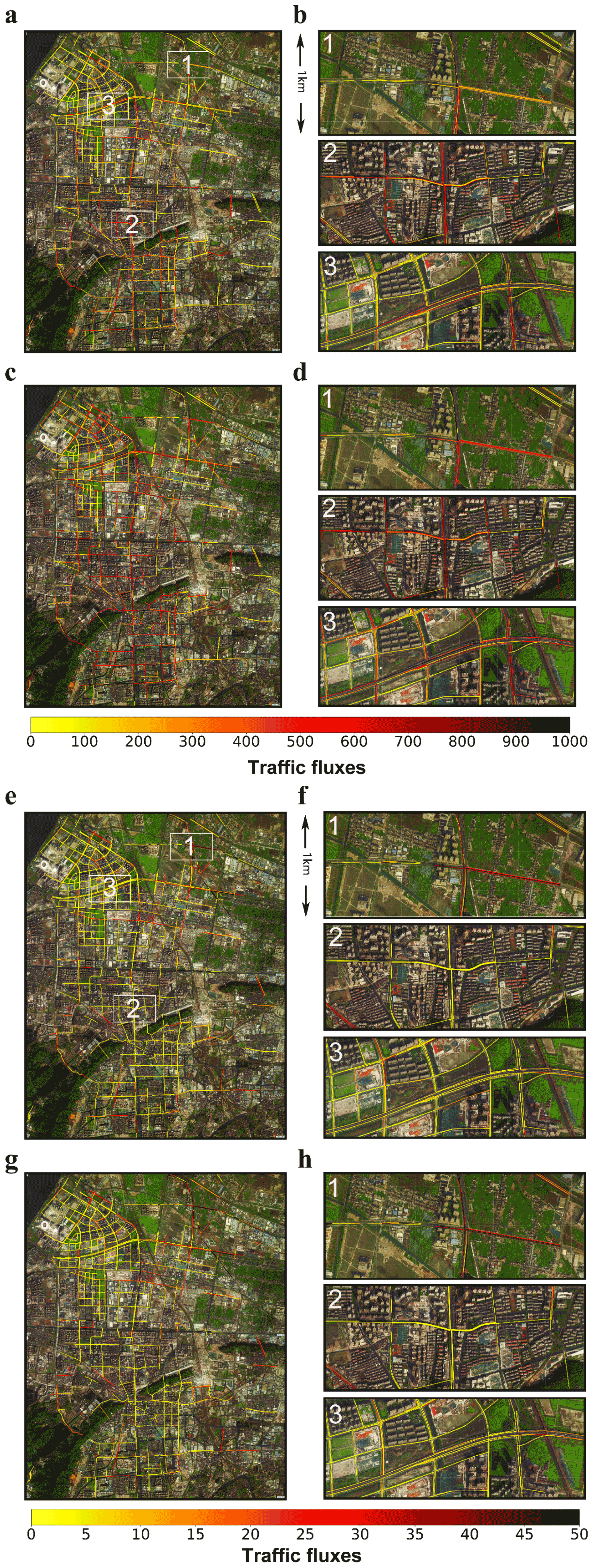
Figure 3 Hyperfine-resolution mapping of observed traffic fluxes. (a) Hourly average traffic fluxes in each road segment based on 2-month traffic monitoring data over the entire district and (b) for three indicative 1 km² urban zones therein. The panels (c) and (d) are the same as (a) and (b) but for the hourly average traffic fluxes during the morning and evening rush hours (from 07:00 to 09:00 and from 16:30 to 18:30 local time) on weekdays (from Monday to Friday). The panels (e) and (f) are as the same as (a) and (b) but for the hourly average traffic fluxes of HDVs and HDTs. The panels (g) and (h) are as the same as (c) and (d) but for the morning and evening rush hours on weekdays. The indicative zones are marked by white rectangles in (a), and their spatial scales are presented in (b). Illustrative traffic hotspots (white-outlined rectangles) are also annotated in (a), including Tonghui North Road, Hongda Road, Shixin North Road, Shanyin Road, and Airport Road. Map data © 2021, Gaode Map.

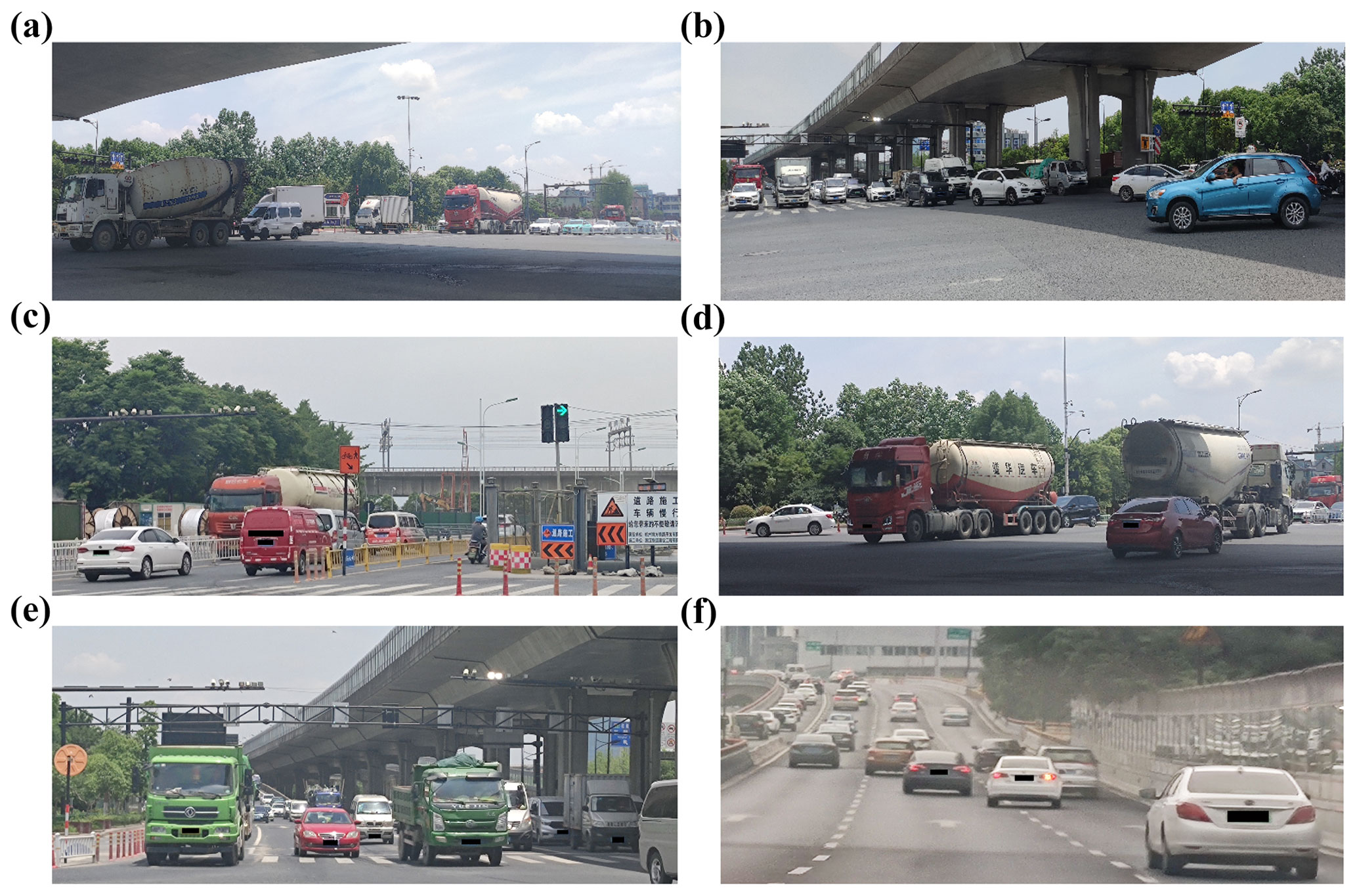
Figure 4 Imagery analysis for illustrative traffic hotspots. (a, b) Over the hotspots in the urban zones, frequent large traffic fluxes are identified on major arterial roads and their intersections. (c) Constructions in the middle of the roads also lead to traffic congestion. (d, e) Morning and afternoon traffic rushes further exacerbate traffic congestion. (f) Over the highways, the hotspots are related to large traffic fluxes of MDTs and HDTs. The vehicle license plates are pixelated. The hotspot locations are presented in Fig. 3.

Second, the hourly average traffic fluxes on weekdays were close to those on weekends (Figs. 3 and S3). Nevertheless, the variation tendencies displayed a distinct picture during different moments between weekdays and weekends (Fig. S2). On weekdays, the diurnal traffic fluxes showed dramatic fluctuations, two peaks at 07:00 and 17:00, obviously related to the morning and evening rush hours. We noted that such temporal peaks enhanced extensive spatial hotspots, spatially consistent with the above hotspots based on the hourly average data but quantitatively more prominent (Fig. 3). This was because the morning and evening rushes exacerbated the traffic congestion (Fig. 4). By comparison, the variation extent on weekends was slightly lower than on weekdays and the early peak appeared 2 h later (Fig. S2). Overall, the maximum peak on weekends barely hit roughly 96.46 % of those on weekdays. Spatially, the hotspots of the traffic fluxes on weekdays were mostly consistent with those on weekends but more variable, reflecting frequent casual travels (Fig. S3). Collectively, the fine-scale spatiotemporal patterns of traffic fluxes over the entire district, particularly the hotspots, relied more on those on weekdays.

Third, significantly strong correlations were found between the traffic speeds and fluxes spatially and temporally. Following the traffic fluxes, the simultaneous vehicle-specific speeds fluctuated substantially throughout the day (Fig. S2). When the traffic fluxes peaked in the morning and evening rushes, the vehicle-specific speeds were expected to be at rock bottom. Although the peaks changed from weekdays to weekends, the valleys kept following such peaks. Spatially, the traffic flux hotspots likely determined the traffic speed hotspots, particularly in the morning and evening rush hours (Fig. S4). In contrast, the vehicle categories were independent of the traffic fluxes. Their diurnal variations showed relative stability, even for different road types, after the morning rush hours (Figs. S2 and 3). On the other hand, the HDVs and HDTs peaked in the early hours of the morning (i.e., from 01:00 to 05:00). Besides, a striking picture lay in the spatial distributions (Figs. 3 and S5). Four types of vehicle, including LDVs, MDVs, LDTs, and MDTs, were concentrated on (98.52 %) the arterial and residential roads, while the rest of the vehicle categories, i.e., HDVs and HDTs, were concentrated on (3.61 %) the highways. Figure 3 details fine-scale spatial distributions of HDVs and HDTs for three indicative highway zones (∼1 km²). Therein the spatial hotspots were scattered extensively. According to the imagery analysis (Fig. 4), the traffic congestion attributed to the large traffic fluxes of HDVs and HDTs should be the unique driver. Therefore, the fleet compositions would also affect emission distributions significantly, particularly over fine-scale zones.

3.2 Characteristics of on-road vehicle emissions

We established a hyperfine-resolution on-road vehicle emission inventory and captured the emission hotspots (Figs. 5 and S6 in the Supplement). Overall, the hourly average emissions were summed up based on the classified roads (Table S1 in the Supplement). It was clear that the emission intensities on the arterial roads, residential streets, and highways followed a descending order, although the residential streets were of the longest length and the largest traffic fluxes. The leading cause was the difference in vehicle categories in different road types (Table S1). For instance, we estimated that the hourly average NO_x emission intensities on the arterial roads, residential streets, and highways were 157.76, 135.22, and 107.83 g km⁻¹, respectively. For the highways, the hourly average traffic fluxes were 10 277, accounting for 1.99 % of the total amount, while their emissions amounted to more than 2.04 % of the total emissions.

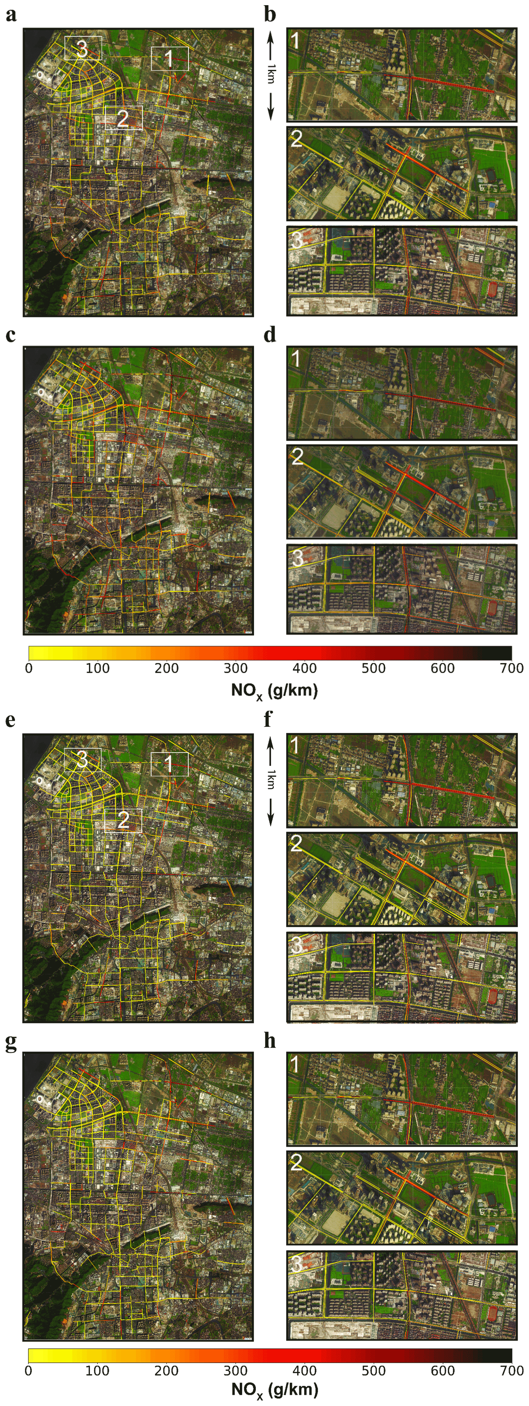
Figure 5 Hyperfine-resolution mapping of on-road vehicle emissions. (a) Hourly average on-road vehicle NO_x emissions for each road segment based on 2-month traffic monitoring data for the entire district and (b) for three indicative 2.5 km² urban zones therein. The panels (c) and (d) are as the same as (a) and (b) but for the hourly average emissions during the morning and evening rush hours (from 07:00 to 09:00 and from 16:30 to 18:30 local time) on weekdays (from Monday to Friday). The panels (e) and (f) are as the same as (a) and (b) but for the hourly average emissions of HDTs and HDVs. The panels (g) and (h) are as the same as (a) and (b) but for the hourly average emissions of HDTs and HDVs during the morning and evening rush hours on weekdays. The indicative zones are marked by white rectangles in (a). Map data © 2021, Gaode Map.

From the temporal perspective, on-road vehicle emissions of CO, HC, NO_x, and PM_2.5 showed similar trends all day (Fig. S7 in the Supplement). For instance, the daytime NO_x emissions accounted for approximately 85.90 % of the daily total emissions. Moreover, the NO_x emissions varied throughout the day but reached agreement among the different road types (i.e., the arterial roads, residential streets, and highways). Yet, there was an apparent difference between emissions on weekdays and those on weekends. Similarly to the temporal variations in the traffic fluxes on weekdays, those in on-road vehicle emissions also peaked in the morning and evening rush hours. In turn, such temporal patterns were indistinct on weekends.

Spatially, the high hourly average emissions with the unprecedented hyperfine resolution spread all over the district (Figs. 5 and S6). Such a spatial pattern was distinct from previous results that generally show decreases from the center to the periphery with a radiating structure (Jing et al., 2016; Yang et al., 2019). It was mostly associated with the spatial patterns of the traffic fluxes and vehicle categories (Figs. 3 and S4). Specifically, the high emissions at the center were mainly attributed to the high traffic fluxes and low traffic speeds. Note that, on the border of the district, the emission intensities in the residential streets far exceeded (>436.65 %) those in the neighboring highways. This divergence could be interpreted by the spatial emission distributions of different vehicle categories (Figs. 3 and S5). For instance, the emissions of HDVs and HDTs in the residential streets contributed the most (79.79 %), much more than those (1.34 %) in the neighboring highways.

3.3 Emission hotspots and drivers

The emissions of each pollutant (i.e., CO, HC, NO_x, and PM_2.5) generally peaked at the major road intersections, leading to the spatial emission hotspots (Figs. 5 and S6). The highest hourly average emissions occurred at the intersection of two arterial roads (i.e., Shixin North Road and Shanyin Road), where the measurement monitored the largest traffic fluxes (Fig. 3).

At broader spatial scales, these hotspot emissions varied substantially among different road types. For instance, the hourly average emissions for the hotspots in Tonghui North Road and Hongda Road (i.e., arterial roads) were approximately consistent with those in Benjing Avenue and Hongni Road (i.e., residential streets) (Figs. 5 and S6, arterial roads vs. residential streets gives 374.91 vs. 216.12 g km⁻¹ for CO, 48.90 vs. 34.13 g km⁻¹ for HC, 180.61 vs. 348.38 g km⁻¹ for NO_x, and 7.41 vs. 15.81 g km⁻¹ for PM_2.5). In contrast, the hotspot emissions on the arterial roads and highways were substantially elevated above the residential levels. The hotspot emissions on the highways (arterial roads) exceed those on the residential roads by a factor of 2.1 (2.3) for CO, by a factor of 1.4 (2.6) for HC, by a factor of 0.9 (1.1) for NO_x, and by a factor of 0.8 (1) for PM_2.5. Therein, emission hotspots for a given highway road were typically intensive and evident in several areas of Xiaoshan District (Fig. 5). For instance, we estimated consistently higher (1.2–2 times) emission levels on a highway (i.e., Airport Road) than on the neighboring residential street (i.e., Wenming Road) (Fig. S8 in the Supplement). More importantly, the diurnal emission hotspots remained stable spatially (Fig. S9 in the Supplement), the hourly spatial patterns of which were roughly consistent with the hourly average level (Figs. 5 and S6). However, the emission intensities of the hotspots varied during different moments between weekdays and weekends (Fig. S10 in the Supplement). The higher emissions of hotspots typically appeared at 08:00 and 18:00 local time on weekdays and were 2.2–3.4 times larger than the hourly average level.

The indicative hotspots over the urban zones generally stretched for 100–200 m (Fig. 5). Over the short length of the transects, the hourly average emissions rose and fell by more than 2.2 times. From the hotspot cores outwards, the hourly average emissions consistently followed “distance–decay” relationships (Fig. 6). An unconstrained three-parameter exponential model, $E\left(d\right)=\mathit{\alpha }+\mathit{\beta }\exp (-\mathrm{3}d/k)$, reproduced the emission–distance relationship E(d) with high fidelity (r²=0.96). Specifically, the isotropic parameter d reflected the distance to the hotspot cores (m); the background parameter α represented the background emissions far from the hotspots (d→1000 m); the parameter β represented the emission increment resulting from proximity to the hotspots; the decay parameter k governed the spatial scale over which emissions relaxed to α. For all pollutants, estimated values of (α+β) approached a constant (1.0), indicating that the combined contribution of the background and the near-hotspot increment approached the hotspot emission levels.

Figure 6 shows the decay patterns of the hourly average emissions over urban zones on weekdays. These results reflected the hourly average emission ratios (normalized at the hourly average emissions of the hotspots) from hotspots outwards as a function of the distance (d). Note that the ratios of the hourly average traffic fluxes and vehicle category proportions were calculated in the same way.

Figure 6 Decay of on-road vehicle emissions, traffic fluxes, and vehicle categories from indicative hotspots outwards on weekdays. (a–d) Points denote the ratio of hourly average emissions (NO_x, CO, HC, and PM_2.5) over different road types at a given distance from hotspots to hourly average hotspot emissions. Error bars present standard deviations. An unconstrained three-parameter exponential model reproduces the decay relationships with high fidelity. The isotropic parameter d reflects the distance to the hotspot cores (m); the background parameter α represents the background emissions far from the hotspots (d→1000 m); the parameter β represents the emission increment resulting from proximity to the hotspots; the decay parameter k governs the spatial scale over which emissions relaxed to α. The panels (e) and (f) are the same as (a) but for traffic fluxes and the vehicle category proportions, respectively.

Consistent with expectations about the speed-dependent emission factors (Fig. S1), our estimated distance–decay relationships were sharpest for NO_x, intermediate for HC and PM_2.5, and most shallow for CO. In theory, comprehensive traffic profiles underlay the estimated hotspot emissions. To elucidate determinants of the emission hotspot patterns, we mined those traffic data (Figs. 3, 5, and S6). As expected, we found that the traffic fluxes largely shaped the spatial emission hotspot patterns over the arterial and residential roads. Besides, the specific vehicle categories (i.e., HDVs and HDTs) also play a key role.

For the emission hotspots on the highways, the traffic fluxes and emissions were both distance-dependent and applicable to the distance–decay exponential models while the vehicle categories were consistently stable (Fig. 6). This proves that the traffic fluxes played a cardinal role in determining the spatial emission hotspot patterns over the highways. In contrast, on the arterial and residential roads, coincident peaks of the specific vehicle categories (i.e., HDVs and HDTs) and traffic fluxes corresponded in space to the emission hotspots (Fig. 6). This reveals that, besides the traffic fluxes, the specific vehicle categories (i.e., HDVs and HDTs) also substantially contributed to the high emissions over the arterial and residential roads.

3.4 Impacts of traffic control scenarios

Four scenarios (i.e., S1–S4) demonstrated substantial impacts of traffic management on spatiotemporal traffic states (Fig. S11 in the Supplement). Thereof the S1 and S2 scenarios focused on reducing the traffic fluxes, while the S3 and S4 scenarios gave full consideration to not only the traffic fluxes but also the fleet compositions (Table 1). Without strict traffic restrictions, the S1 scenario only reduced the traffic fluxes by 3.82 % and showed no significant effects on the traffic flux hotspots. On this basis, the traffic fluxes were further decreased by 9.56 % under the S2 scenario. Most of the traffic flux hotspots vanished. Under the S3 scenario, the fleet compositions were changed evidently over the highways, where HDTs and HDVs were removed. The S4 scenario combined the exclusive settings in the S2 and S3 scenarios and thus realized their consequences. This scenario achieved further decreases in the traffic fluxes (51.3 %).

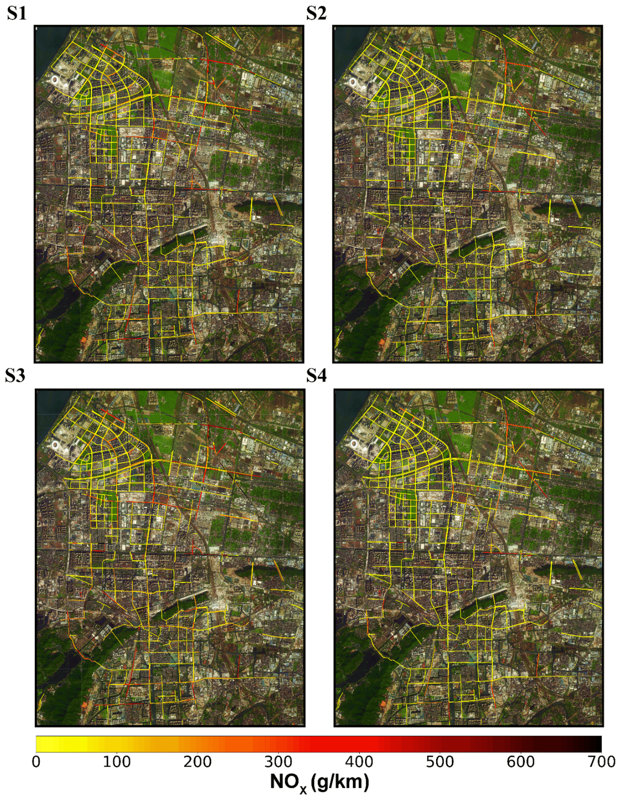
Figure 7 Impacts of traffic control strategies (i.e., S1–S4) on daily average on-road vehicle NO_x emissions. Map data © 2021, Gaode Map.

This study estimated that the daily average on-road vehicle emissions were 3.40 t for CO, 0.482 t for HC, 2.306 t for NO_x, and 0.097 t for PM_2.5 (Figs. 7 and S12 in the Supplement). Under the S1 scenario, the daily average emissions decreased by small percentages (i.e., 3.74 % for CO, 3.43 % for HC, 3.13 % for NO_x, and 3.08 % for PM_2.5). Compared with the S1 scenario, the S2 scenario led to significant reductions over the arterial and residential roads (i.e., 9.34 % for CO, 8.59 % for HC, 7.83 % for NO_x, and 7.69 % for PM_2.5). This represents the effects of strict traffic flux controls on on-road vehicle emissions, particularly over the urban zones. The S3 scenario reveals that the HDVs and HDTs were responsible for a major part (15.94 %–57.50 %) of CO, NO_x, PM_2.5, and HC emissions over the highways. On this basis, the S4 scenario adopted comprehensive traffic controls, thus reducing roughly additional emissions (i.e., 50.77 % for CO, 67.44 % for HC, 82.72 % for NO_x, and 84.20 % for PM_2.5). As a result, the emission hotspots over all roads were mostly removed. Note that these traffic control scenarios should also alter other traffic parameters (e.g., vehicle-specific speeds). Hence, to further reproduce the feedbacks of traffic states, we should introduce more realistic experiments.

3.5 Comparison with other inventories

The localized emission inventory over Xiaoshan District is still lacking. MEICv1.3 for 2016 and HTAPv2.2 for 2010, as state-of-the-art conventional emission inventories provide a valuable opportunity to evaluate our results (Fig. S13 in the Supplement) (Janssens-Maenhout et al., 2015; Li et al., 2017). It should be noted that the spatial resolution of MEICv1.3 and HTAPv2.2 was roughly $\mathrm{0.25}{}^{\circ }\times \mathrm{0.25}{}^{\circ }$ and $\mathrm{0.1}{}^{\circ }\times \mathrm{0.1}{}^{\circ }$, respectively. Hence, their total emissions over Xiaoshan District were re-aggregated with area-weighting. It was clear that the monthly average on-road vehicle emissions in this study were significantly lower than those in MEICv1.3 and HTAPv2.2 (i.e., in MEIC, 14.8 % for CO, 30.1 % for HC, 40.1 % for NO_x, and 19.7 % for PM_2.5. in HTAP, 22.4 % for CO, 44.5 % for HC, 67.7 % for NO_x, and 29.1 % for PM_2.5). This could be attributed to the persistent on-road vehicle emission mitigation measures in China. Moreover, owing to the limitation of the spatial resolution, these conventional inventories were incapable of depicting the emission hotspots over Xiaoshan District. Such limitations could be propagated to previous chemical transport model (CTM) simulations driven by those conventional inventories, thus making them unable to reproduce the fine-scale on-road vehicle emissions.

3.6 Stability analysis

Through systematic subsampling of our weekday emission dataset, we found that 15–30 weekdays were sufficient to reproduce key spatial patterns with good precision and low bias (Fig. 8). The following trends hold: a small number of drive days (N<5) typically resulted in a poor approximation of long-term spatial patterns from the full dataset, with generally low precision (γ²) and high bias (CV-RMSE). However, each additional sampling day resulted in a substantial improvement in γ² and CV-RMSE.

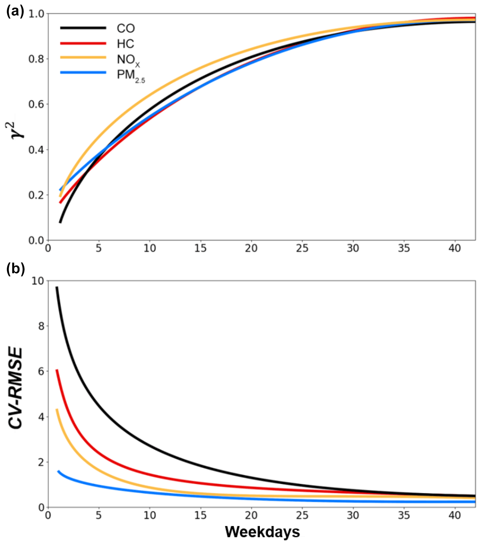
Figure 8 Scaling analysis through systematic subsampling. Using the systematic subsampling algorithm described in Sect. 2.4, we investigated the relationship between the number of drive days and metrics of precision and bias. (a) Mean subsampled γ² versus the number of unique weekdays for CO, HC, NO_x, and PM_2.5. (b) Mean subsampled coefficient of variation of root-mean-square errors (CV-RMSE) versus the number of unique weekdays for CO, HC, NO_x, and PM_2.5.

For our dataset, diminishing returns for improvement in γ² set in at 15–25 drive days, with the mean γ² for NO_x and PM_2.5 approaching 0.7 after 15 weekdays and approaching 0.9 after 30–35 weekdays. We found that ICC values ranged from 0.72 to 0.91 for all pollutants (Table S2 in the Supplement). This indicates that our measurement-based long-term spatial patterns were robust to stochastic variability among those samples. Average values of the ICC (Fig. S14 in the Supplement) were generally high for 10 or fewer weekdays, indicating that stochastic temporal variability from a small number of weekdays did not obscure an overall spatially dominated emission pattern. Note that our sampling was restricted to weekday conditions, but spatial patterns may differ at other times (weekends) due to casual trips. Future work may reveal whether similar scaling considerations hold over a broader range of conditions.

4 Conclusions

This work establishes a hyperfine bottom-up approach to reveal a unique on-road vehicle emission pattern at a spatial resolution 1–3 orders of magnitude higher than current emission inventories. In particular, all-around traffic monitoring (including traffic fluxes, vehicle-specific categories, and speeds) is interconnected via an intelligent transportation system (ITS) over Xiaoshan District in the Yangtze River Delta (YRD) region. This enables us to calculate single-vehicle-specific emissions over each fine-scale (10 m–1 km) road segment. Consequently, the most hyperfine emission dataset of its type is achieved, exposing widespread and persistent emission hotspots. More importantly, this map depicts significantly sharp small-scale variability, up to 8–15 times within individual hotspots, attributable to distinct traffic fluxes, road conditions, and vehicle categories. Once all kinds of vehicles comply with the even–odd rule over the entire district, more than 50 % of the emissions are reduced. By comparison, our results are lower (>14.8 %–67.7 %) than those in the conventional emission inventories (i.e., MEICv1.3 and HTAPv2.2). Through systematic subsampling of our weekday emission dataset, we find that 15–30 weekdays are sufficient to reproduce key spatial patterns with good precision and low bias.

In our model framework, the traffic fluxes are measured accurately. By comparison, the emission factors have larger uncertainties. This is because although they are obtained from the local official vehicle inspection and maintenance (I/M) datasets, some assumptions are inappropriate. For instance, the emission factors are measured in lab circumstances, possibly unsuitable for real-world conditions (Seo et al., 2021). Besides, they are calculated as a function of the vehicle categories and speeds (Fig. S1), without consideration of fuel-dependent discrepancies. Instead, we assumed that, in this study, HDVs and HDTs are diesel-driven, while other vehicle categories are fueled by gasoline. Also, the effects of vehicle ages were ignored. Such assumptions are consistent with previous studies (Yang et al., 2019; Zhou et al., 2017). Future introductions of constraints via near-road emission measurements would decrease such uncertainties.

This work proposes a straightforward emission model framework that can provide several orders of magnitude more spatial information. As shown in our results, this approach could be extended to nationwide megacities if comprehensive traffic conditions are fully measured and interconnected via the ITS. However, its costs are significantly higher than those of previous attempts. To this end, more flexible data collection from low-cost sensors, such as those on cell phones, taxis, and public transit, could substantially lower the costs of monitoring instruments. Furthermore, advances in open-source traffic platforms that can complete those big data interconnections would further decrease the costs. In addition, as demonstrated in Sect. 3.6, our approach, coupled with data reduction algorithms, might also enable high-resolution emission mappings. This indicates an application potential of our approach for middle-sized and small cities where robust traffic monitoring infrastructures are absent.

Overall, routine accessibility of hyperfine-resolution on-road vehicle emissions could have transformative implications for air pollution control, urban management and policymaking, epidemiology, and public awareness (Daellenbach et al., 2020; Dedoussi et al., 2020; Geng et al., 2019; Nyhan et al., 2016; Yang and Zhang, 2018; Zeger et al., 2000). By pinpointing localized emission hotspots, these data may provide new opportunities for policymakers. Specifically, our results can replace the coarse-grid ($>\mathrm{1}\times \mathrm{1}$–25×25 km²) emission inventory (Janssens-Maenhout et al., 2015; Li et al., 2017; Zhang et al., 2013) as the input of the CTM. Comparably, the meteorological input should also be sufficiently hyperfine, which thus needs to account for large eddy simulations (e.g., WRF-LES) (Zhong et al., 2020). In so doing, dispersion models (e.g., AERMOD) (Yang et al., 2019), instead of full CTMs (Mehmood et al., 2020; Wong et al., 2012; Yu et al., 2014), are sufficient to resolve street-level gradients of air pollution concentrations. Through combination with CTM outputs and near-road air quality measurements (Apte et al., 2017; Grange et al., 2017; Jiang et al., 2018; Yang et al., 2018), the hyperfine-resolution scanning of responses of air quality to emissions becomes possible. This would help in the understanding of highly nonlinear air pollution mechanisms, such as O₃–VOC–NO_x relationships (Li et al., 2019), and thus optimize mitigation policies. Besides, the resulting hyperfine-resolution maps of air pollutant concentrations can help address exposure misclassifications and even directly alter personal behaviors, such that real-time traffic navigation data can now inform individual driving patterns. In addition, these hyperfine-resolution emission and air quality maps might result in broader societal consequences, including in terms of urban land-use decisions, ecological planning, and political economy.