the Creative Commons Attribution 4.0 License.
the Creative Commons Attribution 4.0 License.
 | 17 Nov 2021
A sulfur dioxide Covariance-Based Retrieval Algorithm (COBRA): application to TROPOMI reveals new emission sources
Nicolas Theys
Vitali Fioletov
Isabelle De Smedt
Christophe Lerot
Chris McLinden
Nickolay Krotkov
Debora Griffin
Lieven Clarisse
Pascal Hedelt
Diego Loyola
Thomas Wagner
Vinod Kumar
Antje Innes
Roberto Ribas
François Hendrick
Jonas Vlietinck
Hugues Brenot
Michel Van Roozendael
Sensitive and accurate detection of sulfur dioxide (SO2) from space is important for monitoring and estimating global sulfur emissions. Inspired by detection methods applied in the thermal infrared, we present here a new scheme to retrieve SO2 columns from satellite observations of ultraviolet back-scattered radiances. The retrieval is based on a measurement error covariance matrix to fully represent the SO2-free radiance variability, so that the SO2 slant column density is the only retrieved parameter of the algorithm. We demonstrate this approach, named COBRA, on measurements from the TROPOspheric Monitoring Instrument (TROPOMI) aboard the Sentinel-5 Precursor (S-5P) satellite. We show that the method reduces significantly both the noise and biases present in the current TROPOMI operational DOAS SO2 retrievals. The performance of this technique is also benchmarked against that of the principal component algorithm (PCA) approach. We find that the quality of the data is similar and even slightly better with the proposed COBRA approach. The ability of the algorithm to retrieve SO2 accurately is further supported by comparison with ground-based observations. We illustrate the great sensitivity of the method with a high-resolution global SO2 map, considering 2.5 years of TROPOMI data. In addition to the known sources, we detect many new SO2 emission hotspots worldwide. For the largest sources, we use the COBRA data to estimate SO2 emission rates. Results are comparable to other recently published TROPOMI-based SO2 emissions estimates, but the associated uncertainties are significantly lower than with the operational data. Next, for a limited number of weak sources, we demonstrate the potential of our data for quantifying SO2 emissions with a detection limit of about 8 kt yr−1, a factor of 4 better than the emissions derived from the Ozone Monitoring Instrument (OMI). We anticipate that the systematic use of our TROPOMI COBRA SO2 column data set at a global scale will allow missing sources to be identified and quantified and help improve SO2 emission inventories.
- Article
(21407 KB) - Full-text XML
-
Supplement
(31408 KB) - BibTeX
- EndNote


Sulfur dioxide (SO2) in the atmosphere rapidly oxidizes into sulfuric acid and sulfate aerosols, which have environmental effects ranging from local and long-range air pollution to global climate impact. SO2 is released into the atmosphere from anthropogenic activities, due to fossil fuel burning (coal, oil and gas) and smelting, and from natural sources, mainly volcanoes. Satellites provide a viable means to monitor global SO2 emissions and assess their environmental impacts. Since the late seventies, SO2 vertical column densities (VCDs) are provided by several ultraviolet (UV) polar-orbiting nadir instruments, namely the Total Ozone Monitoring Spectrometer (TOMS; Krueger, 1983), Global Ozone Monitoring Experiment (GOME; Eisinger and Burrows, 1998; Khokhar et al., 2005), SCanning Imaging Absorption spectroMeter for Atmospheric CHartographY (SCIAMACHY; Afe et al., 2004), Ozone Monitoring Instrument (OMI; Krotkov et al., 2006; Yang et al., 2007, 2010; Li et al., 2013; Theys et al., 2015), Global Ozone Monitoring Experiment-2 (GOME-2; Nowlan et al., 2011; Rix et al., 2012; Hörmann et al., 2013), Ozone Mapping and Profiler Suite (OMPS; Yang et al., 2013; Zhang et al., 2017), and TROPOspheric Monitoring Instrument (TROPOMI; Theys et al., 2017). From the various data sets, a remarkable trend emerges in the ability of successive sensors to detect weaker and more localized emissions. This is in part due to the better spatial resolution and performance in terms of noise of the modern UV spectrometers (see for example Fioletov et al., 2013, and Theys et al., 2019), but also from advances in retrieval techniques. In particular, the principal component algorithm (PCA) applied to OMI (Li et al., 2013, 2020a) and OMPS (Zhang et al., 2017) proved to be a very efficient method to reduce retrieval noise and biases and thus to increase the sensitivity of the retrievals to weak SO2 emissions to 30–40 kt yr−1. This enabled major improvements in bottom-up emissions inventories (Liu et al., 2018) and detection of missing SO2 emission sources (Fioletov et al., 2016; McLinden et al., 2016).
TROPOMI, launched in October 2017 onboard the ESA and Copernicus Sentinel-5 Precursor (S-5P) platform, is an atmospheric mission with a dedicated focus on the tropospheric composition (Veefkind et al., 2012). With a spatial resolution as good as 3.5×5.5 km2 per ground pixel (3.5 × 7 km2 before August 2019), it is specifically designed to monitor atmospheric constituents from urban to global scales. The first observations of SO2 by TROPOMI were focusing on relatively large volcanic sources and indeed revealed the great potential of the instrument to provide information about global volcanic SO2 degassing with high resolution and unprecedented sensitivity (Theys et al., 2019; Queißer et al. 2019). However, further investigation of anthropogenic and volcanic SO2 sources using TROPOMI revealed problems with the current TROPOMI SO2 retrievals for weak emission sources (Fioletov et al., 2020). In brief, large-scale and variable VCD biases on the order of 0.25 Dobson units (DU; 1 DU = 2.69 × 10¹⁶ molecules cm−2) are present in the data, which limits their use to medium to large SO2 sources only.
The operational TROPOMI SO2 algorithm is based on the differential optical absorption spectroscopy (DOAS; Platt and Stutz, 2008) technique and essentially works in three steps (details are given in Theys et al., 2017): a spectral analysis yielding SO2 slant column densities (SCDs), an empirical background correction of the SCDs and a radiative transfer calculation of air mass factors (AMFs) to convert the corrected SCD into the VCD output (VCD = SCDAMF). As a matter of fact, the SO2 SCD retrieval is subject to spectral misfits which can lead to systematic offsets. These SCD errors are difficult to correct and arise from imperfect DOAS forward modelling. Here, we propose an alternative spectral fitting approach, named COBRA, which strongly reduces the SO2 SCD biases for the weak SO2 columns and suppresses the need for the post-processing background correction. COBRA is akin to the PCA approach, which constitutes the basis of the OMI and OMPS SO2 operational retrievals (Li et al., 2020b, c). As demonstrated below, COBRA significantly improves the quality as compared with the current TROPOMI DOAS operational SO2 product. The analysis of 2.5 years of data oversampled at high resolution reveals many new SO2 emission sources globally, highlighting the great performance of COBRA in terms of SO2 detection.
The paper is structured as follows. Section 2 describes the algorithm and its practical implementation. In Sect. 3, SO2 retrievals from COBRA are evaluated against other satellite data sets, model results and ground-based observations. Section 4 presents long-term averaged global results. In Sect. 5, we apply an emission inversion scheme to the COBRA SO2 data set and compare with previously estimated SO2 emissions from the TROPOMI operational product. New SO2 emission sources detected by COBRA are discussed. Conclusions are given in Sect. 6.
2.1 TROPOMI
In this study, we use observations from the TROPOMI instrument on the Sentinel-5 Precursor satellite. TROPOMI is a hyperspectral nadir sensor measuring solar radiation back-scattered by the atmosphere and reflected by the Earth, in the ultraviolet, visible, near-infrared and shortwave infrared wavelength regions. TROPOMI delivers column amounts of minor atmospheric constituents, such as O3, NO2, SO2, HCHO, CO and CH4, as well as aerosol and cloud information (Veefkind et al., 2012). The S-5P satellite is a polar orbiting platform crossing the Equator at 13:30 local time. A nearly global coverage is achieved in one day owing to a 2600 km wide swath. The footprint on the ground of the satellite measurement depends mainly on the across-track position in the swath and on the spectral band. For SO2, the ultraviolet spectral band 3 is used, and the swath is divided into 450 across-track positions (also referred to as “rows”). The spatial resolution for the centre of the swath is approximately 3.5 × 7 km2 (across-track × along-track) until 6 August 2019 when the sampling improved to 3.5 × 5.5 km2.
For this work, we analyse data measured between 1 April 2018 and 31 December 2020, and solar zenith angles (SZA) less than 60∘.
2.2 Algorithm description
As mentioned above, the operational TROPOMI SO2 algorithm is based on the DOAS technique, the most widely used method to derive atmospheric trace gas constituents in the UV–visible spectral range. The inverse problem can be expressed (employing the notation of Rodgers, 2000):
where is the optical depth, i.e. the logarithmic ratio of the wavelength calibrated measured intensity (I) and the reference intensity spectrum (Io) over a given wavelength range; x is the state vector including SCDs of relevant trace gases and closure fit parameters (e.g. for broadband effects); K is the forward model matrix with absorption cross sections and other spectra; and ϵ is the measurement noise. The solution can be approximated by least-square fitting:
where S∈ is the measurement error covariance matrix. The latter matrix is most often taken diagonal (no error correlations) or proportional to unity (unweighted least-square). Equations (1) and (2) describe the simplest DOAS approach and are given here for illustration purposes only. In practice, the DOAS problem is fundamentally non-linear in many aspects and DOAS software packages, such as QDOAS (Danckaert et al., 2017), support different non-linear retrieval options (e.g. for wavelength shift and squeeze, or intensity offset), with the aim to improve the quality of the retrievals.
For weakly absorbing tropospheric species, retrieval artefacts are frequent with DOAS (notably for satellite nadir geometry) and are attributed to spectral interferences, imperfect forward model and incomplete treatment of instrumental effects (e.g. polarization sensitivity). For UV nadir SO2 retrievals in particular, biases in the data arise mainly from strong ozone absorption and imperfect treatment of the non-elastic rotational Raman scattering (Ring) effect. It is generally difficult to completely remove these offsets even after applying post-processing background corrections (Theys et al., 2017; Fioletov et al., 2020).
The Covariance-Based Retrieval Algorithm (COBRA) presented here, and illustrated for TROPOMI measurements, aims to correct most of the artefacts in the DOAS SO2 SCDs by optimally retrieving a single parameter: the SO2 SCD.
First introduced by von Clarmann et al. (2001), the retrieval approach was developed by Walker et al. (2011) for nadir observations of SO2 and NH3 from the Infrared Atmospheric Sounding Interferometer (IASI). Then, the technique, also known as hyperspectral range index (HRI), has been further refined and successfully applied to other trace gases and aerosols (e.g. Van Damme et al., 2014; Franco et al., 2018; Clarisse et al., 2019a). The method proved to be very sensitive and led to superior data quality both in terms of precision and accuracy. Surprisingly, this technique has, to our knowledge, never been applied in the UV–visible spectral range.
Starting from Eq. (1), we assume the measurement vector can be linearized around a background SO2-free spectrum :
with ϵbg being the deviation of the SO2-free component of the spectrum relative to the mean spectrum and ϵ being the measurement noise. The SO2 contribution to the measured spectral optical depth is approximated by the product of the instrument slit convolved absorption cross-section vector k (expressed in cm2/molecule) and the SO2 SCD (in molecules/cm2). Here, we use as input of the retrieval the same SO2 absorption cross-section data (Bogumil et al., 2003) and the same approach for the wavelength calibration of the spectra as for the operational TROPOMI SO2 retrievals (see Theys et al., 2017). The only difference is the wavelength interval of 310.5–326 nm (see discussion below).
The basic principle of the method is to consider all contributions to the difference () other than SO2 as an error term (ϵbg+ϵ) with a Gaussian distribution. If one can define an ensemble Y of N measured SO2-free spectra, representative of the total (ϵbg+ϵ) variability, and characterized by a mean measurement vector and a covariance matrix S,
then the solution of the problem is written as
where is the mean SO2 SCD of the ensemble ( by definition). The error on the retrieved SCD is given by the square root of the error covariance of the solution (Rodgers, 2000):
Fundamentally, COBRA generalizes the measurement error covariance matrix of Eq. (2) by incorporating geophysical background spectral variability (including all cross-correlations), variability from the atmosphere or variability induced by instrumental changes.
For spectra where no enhancements of SO2 can be detected, the linearization (Eq. 3) simplifies to
Both sides of the equation have therefore the same probability distribution, and it follows that the covariance matrix associated with ϵbg+ϵ can readily be constructed by applying Eq. (4) on a representative set of SO2-free spectra. The key is to define the ensemble Y such that cancels much of the systematic components of ϵbg.
A remarkable feature of COBRA is its simplicity. The SO2 SCD retrieval in Eq. (5) reduces to a simple dot product between the residue and kTS−1 (skipping the normalization factor ). The vector kTS−1 essentially contains the weights of each wavelength to the retrieved target column amount; the strength of the method relies on the fact that these weights are optimally determined by the measurements themselves. This is in contrast to the DOAS approach which mostly considers all wavelengths equal. Furthermore, DOAS also allows for cross-talks between the state vector elements, which can lead to an increase in the SCD data scatter (in particular for weak absorbers). This is obviously not the case for COBRA, as only a single parameter is retrieved, the SO2 slant column. COBRA has other great advantages that we briefly outline here:
-
Except for the wavelength calibration step, the algorithm does not need a reference spectrum (Io). Indeed, Eqs. (4) and (5) involve differences of logarithmic intensity ratios, and thus Io cancels out. Following the same logic, any constant spectral feature multiplicative to the radiance and shared by the ensemble Y will have no influence on the retrieved SCDs.
-
The analysis of individual spectra with COBRA does not require the fit of a wavelength shift and squeeze, a common (and often time-consuming) practice in DOAS. Beirle et al. (2013) have shown that the effects of spectral shift and squeeze can be linearized and represented by pseudo-absorbers. Therefore, their contributions (and variability) to the optical depth are accounted for by the covariance matrix.
-
The COBRA results display low noise. This is a direct result of the COBRA approach in that the wavelengths with the largest background radiance variability will have the lowest weights on the retrieved SCD (Eq. 5).
-
Very small biases are observed in the COBRA data (see next section). As a consequence, an empirical SCD background correction is not needed.
-
The approach works in principle for any wavelength range. This allows flexibility in case of lower instrumental performance for certain wavelength regions.
-
The covariance matrix S and mean measurement vector can be pre-calculated and the implementation of COBRA then becomes very efficient in terms of processing time (about an order of magnitude faster than DOAS non-linear schemes).
However, the practical implementation for COBRA requires some caution. The main difficulty lies in the definition of the ensemble Y used to construct S (and ). The sample of N spectra should be highly representative of the measurement conditions under consideration, otherwise offsets in the SCDs will likely occur. Also, in principle, the spectra should be uncontaminated by absorption of the trace gas of interest. Finally, N should be large enough to ensure statistically meaningful covariance results.
It should be stressed that COBRA is close in concept to the PCA SO2 algorithm of Li et al. (2013, 2020a). In brief, the PCA scheme characterizes the background radiance variability using a number of leading PC spectra (typically 20–30), instead of a covariance matrix. The SO2 column is then retrieved from the measured spectrum along with the PC fitted parameters. In comparison, COBRA removes the need of having many parameters to fit. Only the SO2 slant column density is determined, and the background radiance variability is fully described by the covariance matrix. In a sense, COBRA can be considered as a generalization of the PCA scheme. It is therefore of great interest to compare the two methods (see Sect. 3.1). With this perspective in mind, the parameters of COBRA for the retrieval of SO2 from TROPOMI have been largely aligned with the PCA algorithm, to facilitate the comparison.
The input spectra for the covariance matrix calculation are analysed separately for each TROPOMI row, to consider the row-dependent characteristics of the instrument. We also treat each orbit individually to account best for the orbit-to-orbit variability. The data are first screened for solar zenith angles larger than 60∘, and to cope with the latitudinal dependence of the total ozone absorption and of the Ring effect, the data are divided into six equal and non-overlapping along-track segments. For each segment, an initial covariance matrix S is derived, and initial estimates of SO2 SCDs are inverted through Eq. (5). In a second step, improved estimates of S and SO2 SCDs are obtained iteratively by removing SO2-contaminated spectra from the ensemble Y. To do this, we use the ratio of the SO2 SCD to its retrieval uncertainty (Eqs. 5 and 6), referred to as the SNR:
A fixed SNR upper value of 1.5 is used for the filtering. This is a rather strict value but tests over pristine regions indicate that this choice does not introduce biases in the SCD data. The number of iterations is set to 4, but in general we already found small changes in the results after 2 iterations. A lower limit on the number N of SO2-free spectra is set to 50. If this limit is reached, because of a major volcanic eruption for example, the SO2 SCD retrieval is entirely skipped for the corresponding row–segment pair. This is a limitation of the current algorithm version, but in the future a better handling of this problem would be possible, e.g. by using a covariance matrix fallback constructed from previously processed orbits. However, the amount of data skipped is small, on the order of 0.025 % in total.
To help the comparison with the PCA SO2 algorithm, we have used a spectral window from 310.5 to 326 nm (instead of 312–326 nm for the TROPOMI operational DOAS product), which includes the same strong SO2 absorption bands as in the spectral range 310.5–340 nm used by Li et al. (2013). This choice is also motivated by the inclusion of the intense absorption band at 310.8 nm, which leads to a further reduction of the noise on the SO2 column by about 25 %. Note that initial tests with the TROPOMI operational algorithm using the 310.5–326 nm window were actually not very successful (large SO2 SCD offsets). On the contrary, with COBRA, we tested both wavelength ranges (310.5–326 and 312–326 nm) and found only small differences between the retrieved SO2 column patterns (Fig. S1 in the Supplement).
In the following sections, SO2 vertical columns will be presented. For the SCD to VCD conversion, we have used air mass factors from the operational product. Note that doing so is not strictly valid because one should expect lower AMFs due to the change in fitting window (from 310.5 to 326 to 312–326 nm). To account for this, we have applied a constant scaling factor of 1.15 to the retrieved SO2 VCDs. Based on radiative transfer calculations, we found this to be a good first-order correction. However, in the future, AMFs shall be recalculated properly. For the cloud filtering and AMF cloud correction, the operational cloud product OCRA/ROCINN CRB is used (Loyola et al., 2018; Compernolle et al., 2021).
As a final note, it should be reiterated that the operational TROPOMI algorithm also handles the retrieval of large SO2 VCDs, by making use of multiple fitting windows (as described in Theys et al., 2017). In this study, we have not applied COBRA on the alternative fitting windows. While there is no fundamental limitation to doing so, COBRA is relevant mostly for low-SO2 columns. All the results presented in the next sections are for situations where the SO2 VCDs are below 5 DU.
3.1 Comparison to satellite observations and CAMS
In order to evaluate the SO2 data from COBRA, it is interesting to first investigate the bias and data scatter over a clean region and compare with the operational product (hereafter referred to as “DOAS”). In Fig. 1, the mean and standard deviation of SO2 slant columns over an equatorial Pacific region are shown for one particular orbit, as a function of the TROPOMI row. As can be seen from Fig. 1a, the DOAS data suffer from SCD offsets in the range of ±0.25 DU, despite the background correction applied. These offsets have a low-frequency dependence component with the across-track position, which is not well understood, but also vary sharply from one row to the next (leading to stripes in the SO2 maps). Given that the background correction is applied separately for each row, this behaviour points to limitations in the correction approach. In contrast, the COBRA results have very small SCD biases (mostly below ±0.025 DU) and no noticeable across-track dependence. It follows that COBRA is a very powerful bias self-correction and destriping scheme. In Fig. 1b, the standard deviations of the SO2 SCD values are shown for both algorithms. Compared to DOAS, it is clear that the data scatter is significantly improved with COBRA, by a factor of 2. It is understood that part of this noise reduction is due to the change in fitting window (Sect. 2.2), but most of the improvement (∼ 75 %) is from the COBRA approach. From Fig. 1, it is clear that the combined reduction of bias and data scatter provided by COBRA over the DOAS results is very significant. From a practical point of view, a factor of 2 improvement of the data scatter means 4 times fewer pixels to average to reach a certain noise level.
In Fig. 1b, we also note a distinct increase in data scatter for the outermost rows, for both DOAS and COBRA. This feature is due to a difference in detector signal binning at the swath edges, which leads to an increase in radiance shot noise. To keep the data of the best quality, we will not use the 50 outermost rows in the rest of the paper.
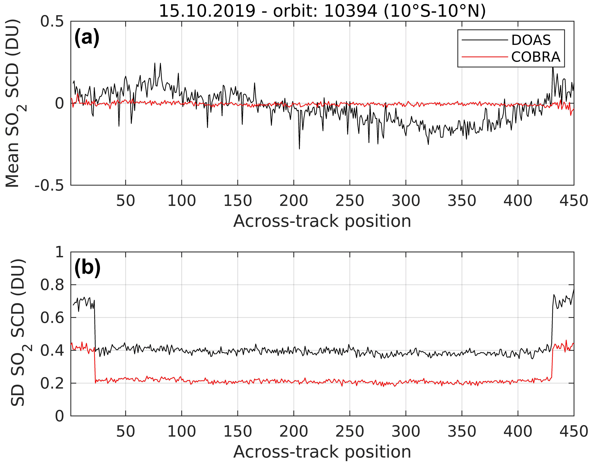
Figure 1(a) Mean SO2 slant columns from (black) DOAS (background corrected) and (red) COBRA for one orbit (10 394 on 15 October 2019) over the equatorial Pacific region (10∘ S–10∘ N), as a function of the across-track position of TROPOMI, (b) same as (a) for the SO2 SCD standard deviation.
Figure 2 compares the DOAS and COBRA seasonally averaged SO2 VCD maps from September to November 2019. The data are gridded at a resolution of 0.1∘ × 0.1∘ and smoothed by a 2-dimensional 5-point box car function. Both DOAS and COBRA results are extracted using identical pixel selection criteria: SZA less than 60∘, radiometric cloud fraction lower than 30 % and TROPOMI rows 26–424. From Fig. 2, several artefacts are evident in the DOAS product. Negative values are found in the tropics and a large-scale positive bias at mid-latitudes. In comparison, COBRA remarkably solves all the systematic biases found in the operational product, whereas the signal from major SO2 sources (e.g. in China, India, the Middle East, South Africa, Central and South America) is nicely preserved. Note that for individual pixels with unambiguous detection of SO2 (typically SO2 VCDs larger than 2 DU), the agreement between DOAS and COBRA is excellent (see e.g. Fig. S2). In Fig. 2, a closer look at the COBRA SO2 map still reveals some negative values for specific locations. For instance, the Garabogazköl Basin near the Caspian Sea is particularly visible. It is characterized by a salt flat with a high albedo. This surface effect is apparently poorly represented in the radiance covariance and leads to the negative values observed in the data.
Retrieval results using the new COBRA are also evaluated in Fig. 2 against a scientific TROPOMI SO2 product generated using the PCA approach. The settings of the experimental TROPOMI PCA SO2 algorithm, including the spectral range and number of iterations, are identical to the operational OMI algorithm with the following exceptions: (1) TROPOMI pixels from each row are grouped into sectors of 20∘ latitude bands, instead of three sectors as in the OMI algorithm; (2) a third-degree polynomial is removed from each Sun-normalized radiance spectrum before PCA analysis; (3) a maximum of 20 PCs are used in the fitting instead of 30 in the current OMI algorithm (Li et al., 2020a); and (4) no attempts were made to reduce TROPOMI retrieval noise over the SAA affected areas. For this exercise, the PCA scheme uses as input the same SO2 absorption cross-section data (Bogumil et al., 2003) as for the DOAS and COBRA retrievals, and the same selection of pixels. Figure 2 also compares the TROPOMI SO2 columns (from DOAS, COBRA and PCA) to the operational OMPS SO2 PCA retrievals NMSO2_PCA_L2 V2 (Zhang et al., 2017; Li et al., 2020c). Although OMPS has a coarser resolution (50 × 50 km2) than TROPOMI, it nonetheless provides useful reference data because it operates on the Suomi National Polar-orbiting Partnership (SNPP) satellite, which flies in loose formation with S-5P (i.e. 3–5 min difference of overpass time). To allow a meaningful comparison, the OMPS pixels were selected similarly to TROPOMI, i.e. with cloud radiance fraction lower than 30 % and OMPS across-track positions 3–34. Note finally that to avoid discrepancies due to different a priori profiles in the TROPOMI and OMPS retrievals, a fixed AMF of 0.4 was used for all four data sets. As can be seen from Fig. 2, an overall excellent agreement is found between COBRA and PCA retrievals, the observed SO2 spatial distributions being essentially the same. However, the OMPS SO2 data set has different patterns over China (possibly due to sampling differences) and also appears noisier than the TROPOMI results (as expected from the smaller number of pixels). When comparing the TROPOMI COBRA and PCA maps, very consistent results are found. Yet, the quality of COBRA seems slightly better than the PCA retrievals. In particular, COBRA is much less sensitive to the South Atlantic Anomaly than PCA data, which exhibit many outliers in the corresponding region. At mid-latitudes, there is also a slight positive bias (of about +0.1 DU on average) and higher noise in the PCA results compared to COBRA.

Figure 2Comparison of seasonal mean SO2 columns for September to November 2019 retrieved from TROPOMI DOAS, COBRA, PCA and OMPS PCA algorithms (from top to bottom). Consistent pixel selection criteria, gridding and retrieval settings are applied (see text). For all four data sets, a fixed AMF of 0.4 is applied.
We have estimated the data scatter for the three TROPOMI data sets, based on measurements from the same orbit over the Pacific as Fig. 1. Results are shown in Fig. 3, as a function of latitude. We find that COBRA has a SCD noise level 20 %–25 % lower than the PCA retrievals, and twice as good as DOAS (as in Fig. 1). Translating the numbers of Fig. 3 in terms of vertical columns for a typical pollution scenario, we estimate the retrieval precision for individual pixels typically to be 0.5–1 DU for COBRA.
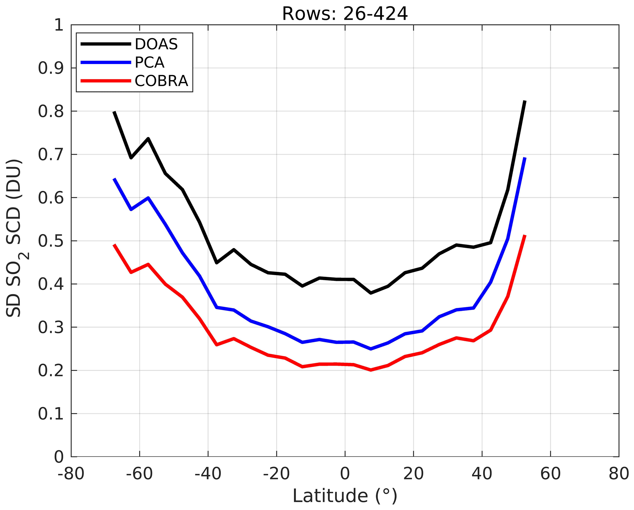
Figure 3Standard deviation of the SO2 slant columns as retrieved from DOAS (black), PCA (blue) and COBRA (red) for one TROPOMI orbit (10 394 on 15 October 2019, same as Fig. 1) for rows 26–424, as a function of latitude (for 5∘ bins).
To further evaluate the overall quality of the COBRA retrievals, the SO2 VCDs can be compared to model data. Here, we have used the output of the Copernicus Atmosphere Monitoring Service (CAMS; https://atmosphere.copernicus.eu/, last access: 20 June 2020) regional model, for September to November 2019. The CAMS regional air quality production is based on an ensemble of nine European air quality models that are run at a resolution of 0.1∘ and produce 4 d, daily forecasts of the main atmospheric pollutants, including SO2. The forecasts and analyses from all nine models are combined in calculating the median value of the individual outputs, which is designated as the ENSEMBLE output and is the field used in this study. The CAMS regional ensemble data were obtained from the Copernicus Atmosphere Data Store (ADS, https://atmosphere.copernicus.eu/data, last access: 20 June 2020). More information about the CAMS regional system can be found on the ECMWF website (https://confluence.ecmwf.int/display/CKB/CAMS+Regional:+European+air+quality+analysis+and+forecast+data+documentation, last access: 20 June 2020). The CAMS regional system used the CAMS-REG-AP_v2_2_1 emissions (reference year: 2015) between June 2019 and February 2020, and the updated CAMS-REG-AP_v3_1 emissions data set (reference year: 2016) since February 2020.
In Fig. 4, seasonal regional maps of S-5P SO2 VCDs over eastern Europe from the DOAS and COBRA schemes are compared to the output of the CAMS regional model, for September to November 2019. From the maps, it is clear that the COBRA results are in much better agreement with the CAMS analysis than the DOAS data. Owing to the quasi-absence of bias and the low noise level, the COBRA data allow better isolation of the emission sources. The agreement between COBRA and CAMS is, however, not perfect and there are several explanations for this. Most of the SO2 emissions in this region are from coal-fired power plants and the emission inventory used by CAMS is likely reflecting neither the actual activity nor the emission mitigation solution (e.g. SO2 scrubbers) at each power plant. Noteworthy is also the absence of SO2 emissions from Mt. Etna in CAMS. Secondly, the AMFs used here are calculated with SO2 profiles from TM5, a different model with a coarser resolution (1∘ × 1∘) than CAMS regional data. Therefore the COBRA and CAMS SO2 columns cannot be strictly compared. Nevertheless, the comparison in Fig. 4 is encouraging. In the future, the COBRA SO2 retrievals together with the corresponding column averaging kernels (Eskes and Boersma, 2003) could be ingested in the CAMS assimilation system to better constrain the model SO2 output and emission estimates.
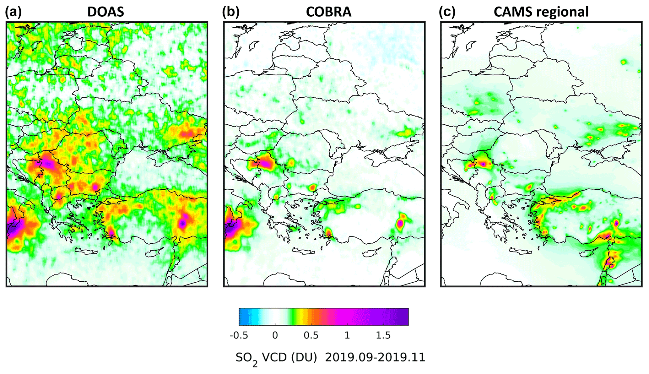
Figure 4Seasonal mean SO2 columns for September to November 2019 from (a, b) TROPOMI DOAS and COBRA retrievals, and (c) simulated by the CAMS regional model. The CAMS data are displayed at the 0.1∘ × 0.1∘ native resolution.
3.2 Comparison to ground-based MAX-DOAS observations
The Multi-Axis DOAS (MAX-DOAS) measurement technique is an established method to retrieve tropospheric trace gas columns and vertical profiles from a sequence of spectral observations performed at various elevation angles above the horizon (Hönninger and Platt, 2002; Tirpitz et al., 2021). MAX-DOAS measurements leverage the fact that low elevation measurements have enhanced sensitivity to atmospheric pollutants in the boundary layer and that the combination of the different elevations carries information on the vertical distribution of the trace gas of interest as well as aerosols. The simplest estimation of the tropospheric VCD from MAX-DOAS measurements is obtained by scaling the differential SCD at a given elevation angle (often 15∘ or 30∘) with an AMF assuming a geometrical light path through the trace gas layer. Recently, more sophisticated approaches have been developed to retrieve the concentration profile in the troposphere using multiple elevation measurements.
Here we compare our TROPOMI SO2 VCD data to MAX-DOAS observations at two sites, both characterized by relatively low-SO2 columns: Xianghe and Mohali (Table 1). In general, the different MAX-DOAS instruments and SO2 retrievals share common characteristics, practices and approaches, and the reader is referred to the publications listed in Table 1 for more detailed information.
For the comparison, we have used a common set of selection criteria for the satellite data. For each day, we selected the TROPOMI pixels within a 25 km radius circle around the station of interest, a strict radiometric cloud fraction threshold of 20 %, SZA lower than 60∘ and AMF larger than 0.2. If the number of retained pixels is larger than 10 then the mean SO2 VCD is calculated and compared to the averaged SO2 column for the MAX-DOAS measurements within ±1 h of the S-5P overpass time.
Regarding the ground-based retrievals, the SO2 VCDs are estimated, for Mohali, using the 15∘ elevation SO2 SCDs and geometrical AMFs. Conversely, the retrieved data for Xianghe consist of SO2 profiles. These are integrated along the vertical to provide the VCDs. Moreover, to make the comparison between MAX-DOAS and TROPOMI more consistent, we have rescaled the TROPOMI VCDs using the satellite averaging kernels (Eskes and Boersma, 2003) and the MAX-DOAS SO2 profiles at Xianghe.
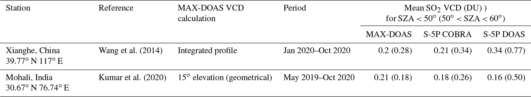
The comparison results between COBRA and MAX-DOAS measurements are shown in Fig. 5a and b, for Xianghe and Mohali, respectively. Overall, the agreement between COBRA and MAX-DOAS data is very good, keeping in mind that the levels of SO2 columns are quite low. The slopes of the regression lines are close to unity. In Table 1, the mean SO2 columns from MAX-DOAS, TROPOMI COBRA and DOAS retrievals are given at each station and for different SZAs. A striking feature of the comparison is that the COBRA results show similar good agreements over a wide range of SZA. It further supports the idea that COBRA yields unbiased results over varying observation conditions. This is in contrast to the DOAS product, which is clearly biased high for high SZA. For completeness, the comparison results between TROPOMI DOAS and MAX-DOAS measurements are shown in Fig. S3, for both Xianghe and Mohali stations. The agreement is clearly not as good as for the COBRA vs. MAX-DOAS comparison, both in terms of the correlation coefficients and slopes of the regression lines.

Figure 5The left panels show comparison of monthly mean SO2 columns from MAX-DOAS and TROPOMI COBRA for (a) Xianghe and (b) Mohali. The grey and pale red dots correspond to the individual days. The right panels show scatter plots of monthly mean SO2 columns of TROPOMI COBRA vs. MAX-DOAS observations. Error bars are the standard errors on the monthly average SO2 columns. The correlation coefficient and slope of the regression line are given as an inset for each plot.
In this section, we present long-term global results from COBRA, based on 2.5 years (April 2018–December 2020) of cloud-free TROPOMI data (radiometric cloud fraction less than 30 %). Using an oversampling technique, a global average SO2 column map at 0.015∘ × 0.015∘ resolution was obtained and smoothed by a 2-dimensional 10-point box car function. Figure 6 shows the resulting SO2 distribution for specific regions, over eastern China, India, the Middle East, South America, South Africa, the US and Europe (the global map is also available in the form of a Google Earth/geotiff file, in the Supplement). Figure 6 also shows the locations of the SO2 sources based on the latest OMI 2005–2019 catalogue (Fioletov et al., 2016), with a total of 588 sites, including power plants, smelters, oil and gas industry sources, and volcanoes. As can be seen, many of the sources of the catalogue are easily identified as SO2 hotspots on the map. Conversely, there is also a significant number of sources in the inventory with no detectable SO2 in the TROPOMI data, but one should keep in mind that the catalogue gathers emission sources since the beginning of the OMI data record in 2005, and several of these sources have ceased operations or decreased drastically their emissions since then (e.g. due to the operation of SO2 scrubbers in coal power plants). To help identify those sources, Fig. 6 shows with a different marker the sources detected by OMI for 2018–2019 (i.e. the sources with emissions above the detection limit, as in Fioletov et al., 2016, and McLinden et al., 2016; see also Sect. 5.2). This is also helpful to highlight the differences in sensitivity, as many sources are detected by TROPOMI but not by OMI.
Generally speaking, the SO2 maps of Fig. 6 are very detailed. Biases over clean regions are remarkably low, and emissions-related patterns with SO2 VCDs less than 0.25 DU are clearly visible in many places. By scrutinizing the SO2 distributions, one can identify numerous sources from the current catalogue but also several potentially new source regions. However, some care must be taken in attributing new sources and relating this to the improved sensitivity of TROPOMI COBRA. First, the catalogue is arguably not resolving the individual sources well for dense regions (e.g. in eastern China and India) and, as a matter of fact, typically reports a total emission estimate of a point-like source for what is in reality a cluster of sources. While the algorithm to handle such clusters of sources exists (Fioletov et al., 2017), it has not been implemented in the catalogue yet. Second, the SO2 catalogue is being populated on a best-effort basis, and a number of emission sources might be missing, in particular for emerging countries where industrial infrastructures are built quickly. Third, SO2 outflow from the strong sources – or clusters of sources – can lead to variations in the map and thus fictitious emission sources. Finally, retrieval artefacts, measurement noise or sampling-related issues can also lead to false source identification. Note that a comprehensive identification and classification of new sources from the COBRA SO2 data is not within the scope of the present study. Here, we aim to discuss plausible new SO2 sources (i.e. not in the OMI catalogue). In Sect. 5.2, we will further demonstrate the excellent performance of COBRA in detecting very weak emissions, for a limited number of sources.
The new identified sources are characterized by low-SO2 column levels in the range 0.05–0.2 DU. For instance, in Fig. 6a we observe hotspots of SO2 from power plants (mostly coal but also likely gas) in North and South Korea, northern Vietnam (near Haiphong), several Chinese provinces (e.g. Hubei, Guangxi, Guangdong), and along the coast of China. In Fig. 6b, several weak emission sources can be isolated in India (e.g. over the western coast and the Indo-Gangetic plain), Pakistan, Bangladesh and Sri Lanka (near the city of Colombo). In the Middle East (Fig. 6c), most of the SO2 emissions are from oil- and gas-related industries, like power plants, gas flaring and refineries. Examples of weak SO2 emissions can be found in Saudi Arabia, Oman, Egypt, Syria (near the city of Damascus) and Iran. In South America (Fig. 6d), new emission sources are popping up, notably in Brazil (near Rio de Janeiro, São Paulo and Porto Alegre), and on both sides of the Andes (in Chile and Argentina). In South Africa (Fig. 6e), in addition to the strong emissions from the coal power plants of the Highveld, a clear SO2 signal is detected over Cape Town. Interestingly, the measured SO2 distribution nicely matches the orography setting. In the US (Fig. 6f), the most striking emission region is the state of California, with enhanced SO2 over the Central Valley and the city of Los Angeles. Over the central and eastern parts of the US, the emissions from power plants have declined dramatically over the last 15 years (Krotkov et al., 2016). However, the data still show enhanced SO2 over some of them. In Europe (Fig. 6g), most of the observed enhanced SO2 correspond to sources already in the catalogue. Still, a number of small spots are found, for example in eastern Europe (Romania, Serbia, Kosovo, Hungary), Germany (near Leipzig), Turkey and Tunisia (Gulf of Gabes). Interestingly, enhanced SO2 is also observed over the Gibraltar Strait and Red Sea, which might result from shipping emissions.
Overall, the SO2 maps of Fig. 6 nicely illustrate the great ability of TROPOMI to detect weak SO2 point emissions sources when analysed using a sensitive approach such as COBRA. Using Google Earth imagery and information on industrial facility locations, we were able to confirm that many features in the SO2 map are real sources. For this, we have also compared our SO2 data to tropospheric NO2 column maps from TROPOMI. An example of comparison is shown in Fig. S4 for a region over Central Asia. There, the SO2 emissions sources in the catalogue are mostly from coal power plants and smelters, in the Xinjiang province (China) and eastern Kazakhstan. As can be seen in Fig. S4, several other SO2 emission hotspots are detected (notably in the Xinjiang province) which clearly coincide with locations with enhanced tropospheric NO2.
Nevertheless, several patterns in the SO2 map (Fig. 6) are hard to relate to point source emissions. In particular, the SO2 signal observed over Cape Town (Fig. 6e) and Los Angeles (Fig. 6f) could be due to area sources rather than point emissions. Over South America (Fig. 6d) and the eastern US (Fig. 6f), the apparent SO2 background is intriguing. It is unclear whether this could be due to real SO2 emissions or not. We also identify several artefacts in the data. Unsurprisingly, biases in the data occur for specific conditions which are under-sampled or not optimally represented by the covariance matrix. These are most often surface-related effects (due to peculiar albedo or elevated terrain). One illustration of this problem is given in Fig. 6c, over the Nile Valley. Although some real SO2 emissions are found in the area, with SO2 VCDs larger than ∼ 0.1 DU, there are also unexpected enhancements in the SO2 column that follow the Nile River. These are probably due to the very dark surfaces there. Similarly, elevated values are also found further South in Sudan and Ethiopia, over vegetated scenes. However, the resulting SO2 VCD biases are overall very small, typically less than 0.04 DU (∼ 1 × 10¹⁵ molecules/cm2), and can be suppressed by a local bias correction or more sophisticated approaches.
As mentioned above, the attribution of new sources based on SO2 maps is not straightforward. Efficient space-based techniques to isolate sources and estimate their emissions do exist (Fioletov et al., 2015; McLinden et al., 2016; Clarisse et al., 2019b). However, applying such methods systematically to the TROPOMI COBRA SO2 data goes beyond the scope of this paper. Instead, in the next section, we will estimate the SO2 emissions for the known largest sources and demonstrate the potential of COBRA for the retrieval of weak emissions, for a limited number of new sites.
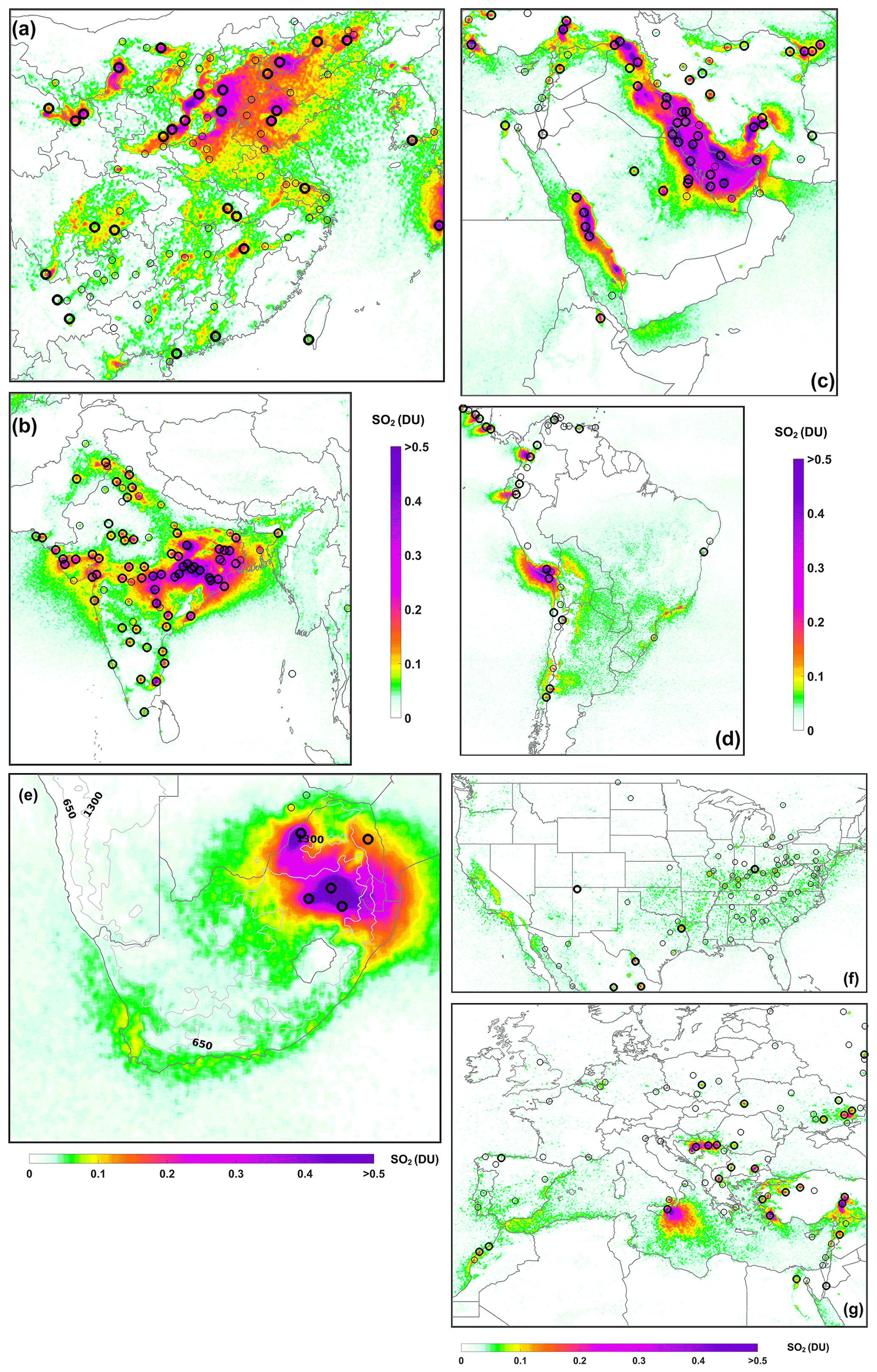
Figure 6Averaged SO2 column (in DU) for April 2018 to December 2020 over (a) eastern China, (b) India, (c) the Middle East, (d) South America, (e) South Africa, (f) the US and (g) Europe. The black circles mark the locations of SO2 sources detected by OMI (in bold for the 2018–2019 period; see text). Due to the massive eruption of Raikoke on 21 June 2019, all data in the Northern Hemisphere, for the 3-month period after the eruption, are filtered out. The grey lines in (e) are the topography isolines (in metres) Note that to further reduce the data scatter, the SO2 map was smoothed by a 2-dimensional 20-point box car function (instead of 10-point function for the other sub-figures).
Satellite observations are being increasingly used to estimate SO2 emissions. In particular, new methods have been very successful in deriving reliable emission rates, and even detecting missing sources, by combining satellite SO2 columns and wind information, without the need for atmospheric chemistry transport models (e.g. Beirle et al., 2014; Fioletov et al., 2016, 2017, 2020; McLinden et al., 2016; Carn et al., 2017). These techniques have been used to derive a global SO2 emissions inventory from OMI observations (Liu et al., 2018). Recently, Fioletov et al. (2020) presented an analysis using the TROPOMI operational SO2 product and found overall consistent results with the OMI emissions estimates. The TROPOMI-based emissions uncertainties were found to be a factor of 1.5–2 lower than the ones from OMI. In this section, we repeat the same analysis using the COBRA SO2 retrievals and investigate the added value of COBRA for the estimation of SO2 emissions. The details of the inversion technique can be found in Fioletov et al. (2015) and references above.
In brief, the method considers a potential point source and applies a wind rotation of the satellite-measured SO2 VCDs around this location. This first step enables all plume dispersion patterns to be aligned along a fixed direction and leads to an improved SO2 detection limit. By contrasting the upwind and downwind averaged SO2 columns, the wind rotation procedure allows confirmation of whether the test location is a real emission source and also correction for a possible bias in the data. Note that for this first step, the retrieved SO2 VCDs are rescaled using site-specific AMFs so that realistic SO2 emission profile shapes (based on the elevation of the site and climatological boundary-layer height) are used for all analysed sources.
The second part of the retrieval method deals with the emission estimate itself. The averaged downwind SO2 field is modelled by an exponential modified Gaussian function which accounts for the SO2 total mass, e-folding time and plume width. From the fitted parameters, the average SO2 emission rate can be derived directly. Here the baseline inversion is, however, not to fit all three parameters but rather to prescribe the e-folding time and plume width, and therefore the only parameter derived from the fit is the SO2 total mass, which is directly proportional to the SO2 emission rate.
5.1 SO2 emissions for large sources
The method was applied to the SO2 data from COBRA for 274 large emissions sources, including power plants, volcanoes, oil and gas sources, and smelters, distributed worldwide. In Fig. 7a, the results are compared to the analysis of Fioletov et al. (2020) using the TROPOMI DOAS product, for the period from April 2018 to March 2019.
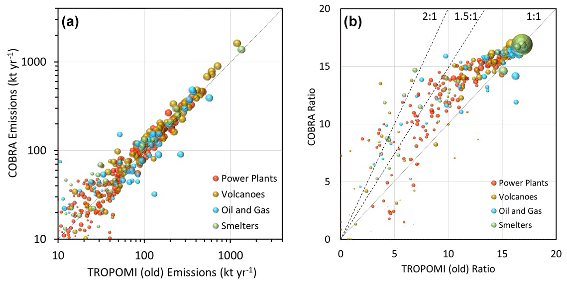
Figure 7(a) Estimated SO2 emissions from TROPOMI, based on the COBRA and DOAS algorithms analysed for power plants, volcanoes, oil and gas industries, and smelter sources. (b) Ratios of the estimated emissions and the corresponding uncertainties. The size of the marker is proportional to the average of COBRA and DOAS (a) ratios between emission value to its corresponding uncertainty and (b) estimated SO2 emissions.
In general, the emission estimates from COBRA and DOAS are fairly consistent for all four source types. For two-thirds of all sources, the differences between DOAS and COBRA emission estimates are within ±3 times the standard deviations of the DOAS-based emissions. However, it was found that the local bias in the satellite data (as derived from the upwind SO2 columns) is much higher with DOAS (∼ 0.25 DU) than with COBRA (∼ 0.05 DU), and that the large differences between DOAS and COBRA emission estimates for some sources are related to problems with the DOAS algorithm. Also, as result of the large improvement in the noise level, the estimated emissions uncertainties are significantly improved with COBRA compared to DOAS, by 20 %–50 % on average (see Fig. 7b).
It should be emphasized though that the improvement of emission uncertainties depends on the emission level. The sources considered here are relatively large sources that have been previously detected by OMI. The TROPOMI COBRA SO2 data set presented in this study combines the advantages of high spatial resolution, low noise level and almost no bias. It has therefore the potential to detect weaker sources (as shown in Sect. 4).
5.2 Detection of weak emissions
It is enlightening to estimate the lowest level of SO2 emission detectable by COBRA. Clearly, it is expected to be dependent on the observation conditions, and generally speaking the best detection limit is obtained for sites with low noise on the SO2 SCDs and the highest measurement sensitivity (i.e. high AMFs). These sites are found at low latitudes and in particular at high elevations or for high albedos. To estimate the emission detection limit, we define the statistical significance of an emission signal as 3 times its standard error. Based on the global sources presented above (Sect. 5.1), we performed statistics using this metric. To avoid biases by the strongest sources, we only considered the sources with estimated emissions less than 50 kt yr−1. The resulting detection limit values are found in the range between 4 and 11 kt yr−1 depending on the AMF, with a mean value of 8 kt yr−1. It is important to realize that this limit of detection is remarkably low, at least twice as good as using TROPOMI DOAS data. It is also a factor of 4 smaller than the detection limit of 30–40 kt yr−1 offered by OMI for the first years of operation (Fioletov et al., 2016; McLinden et al., 2016). This suggests that the TROPOMI COBRA implementation is excellent in exploiting the gain in spatial resolution of TROPOMI compared to OMI (∼ 16 times smaller pixel sizes). This finding is supported by the fact that the noise levels for individual pixels for TROPOMI COBRA and OMI PCA VCDs are similar (not shown; see also Sect. 3 of Fioletov et al., 2020).
In the following, we demonstrate the potential of the TROPOMI COBRA SO2 data set to detect and quantify weak emissions. For this, we use a slightly adapted version of the inversion technique of Sect. 5.1 and illustrate the method on a selection of new emission sources.
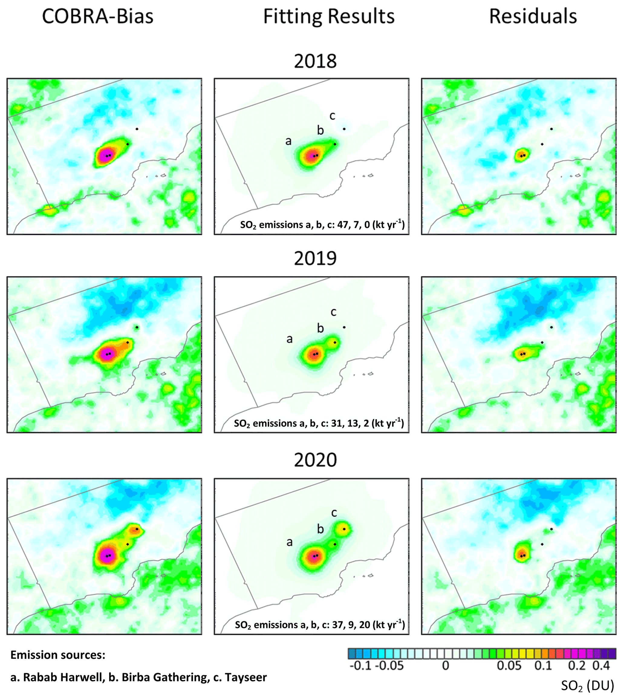
Figure 8The left column shows yearly mean TROPOMI SO2 columns retrieved from COBRA over southern Oman for 2018 (April to December), 2019, 2020 (from top to bottom), and after bias correction for the effect of elevation (see text). Three distinct SO2 spots are discernable from the maps and are the results of emissions from oil and gas fields, referred to as Rabab Harwell, Birba Gathering and Tayseer (centre column), and results of the fitting of TROPOMI SO2 data. The estimated annual SO2 emissions (given in the inset for the three sources) are used to reconstruct the SO2 column field (right column) residuals of the fit or the difference between TROPOMI and fitting results.
The region of interest is the Dhofar governorate in southern Oman. There, the exploitation of oil and gas fields is growing fast, with a number of rapidly evolving projects of exploration and production. In Fig. 8 (left column), the yearly averaged TROPOMI SO2 maps over southern Oman are shown for 2018–2020. One can clearly identify and isolate three main emission locations, namely the Rabab Harwell integrated plant (18.03∘ N, 54.64∘ E), the Birba Gathering station (18.32∘ N, 55.10∘ E) and the Tayseer gas field (18.71∘ N, 55.34∘ E). We note that these emission sources are not listed in any emission inventory and the actual locations of the sources are approximated from available visible imagery (e.g. Google Earth). A noticeable feature in Fig. 8 is the very low observed SO2 column level, in particular over Birba Gathering and Tayseer with SO2 VCDs of 0.03–0.1 DU, reflecting again the great sensitivity of COBRA. To estimate the SO2 emissions from the TROPOMI data, the source method used in Sect. 5.1 has been refined and tuned for this particular case study. A multi-source SO2 emission retrieval was applied as in Fioletov et al. (2017) with one modification: a regression term proportional to the elevation was added to the fit to adjust for a small altitude-related bias in retrieved SO2 (the values were slightly lower over the mountains near the Arabian Sea coast). This multi-source method is motivated by the fact that the sources are close to each other (∼ 50–100 km distance) and the emissions cannot be fitted separately. Here, the approach basically allows for overlaps of the modelled SO2 spatial distributions: the emissions from the individual sources are then adjusted so that the total SO2 modelled field fits best the observed SO2 VCD distribution. In Fig. 8, the results of the fit are shown (centre column), as well as the residuals of the fit (right column). The estimated annual SO2 emissions for the three sources are given in the inset of Fig. 8. Note that for this particular case, the emission detection limit (as defined above) is typically about 6 kt yr−1. For the Rabab Harwell site, the algorithm retrieves rather high and stable emissions over the years, with an average value of about 40 kt yr−1, which is well above the estimated detection limit. Interestingly, the Rabab Harwell site has large residuals of ∼ 0.1 DU for all years. This suggests that the point source representation used here is likely not sufficient to explain the observations, and it is possible that there are many small contributing sources in the area. For the Birba Gathering site, the estimated emissions are much smaller and lie in the range of 7–13 kt yr−1. Yet, there is a good confidence that these emissions are real, given that the estimates are a factor of 1–2 larger than the limit of detection. However, it is clear that the uncertainty of the emission estimates are quite large. For the Tayseer site, an SO2 signal could be detected only recently. In 2019, the estimated emissions are of 2 kt yr−1, i.e. below the detection limit, and in 2020, the SO2 emissions strongly increased to about 20 kt yr−1, probably as a result of a change in operation at the production facility. Finally, note that no significant residuals could be found for either Tayseer or Birba Gathering site, and this suggests a point source behaviour at both sites.
In summary, the analysis over southern Oman of Fig. 8 nicely illustrates the strength of a highly sensitive scheme such as COBRA when applied to a high spatial resolution instrument as TROPOMI. The fact that such low-SO2 emissions can be tracked and quantified with that level of detail is remarkable. Although not shown, the emission inversion scheme was successfully applied not only to the southern Oman sources but also to other test sites, as they were found in the global SO2 map (Fig. 6). The wind-rotation technique when applied to TROPOMI COBRA SO2 data is arguably a promising tool to monitor weak SO2 emissions and track the activity from rapidly emerging production facilities worldwide. However, applying the inversion scheme at the global scale involves a significant effort, as it also requires some level of manual intervention and testing. For instance, the information on source type, location, etc. is typically lacking, and the supporting visible imagery – useful for identifying industrial facilities – is often outdated.
A new spectral fitting method for the retrieval of sulfur dioxide columns in the UV was presented and demonstrated for TROPOMI. Based on a dynamical total measurement error covariance, the method, called COBRA, allows considerable reduction in the noise level (by a factor of 2) and biases present in the current TROPOMI DOAS SO2 operational product. COBRA provides greater sensitivity to low-SO2 columns, and this conclusion is supported by MAX-DOAS observations. Preliminary comparison of COBRA to PCA retrievals suggests similar and even better algorithm performance. The SO2 vertical column precision for individual pixels is in the range 0.5–1 DU. The main limitation of the method relates to the set of spectra chosen to build the covariance matrix, to what extent it is uncontaminated by SO2 and its distribution representative of the observations in the absence of SO2. In particular, very bright or very dark scenes may be poorly represented by the covariance matrix. These conditions (i.e. intensity outliers) can lead to retrieval artefacts. However, the systematic VCD uncertainty (contribution from the COBRA spectral fit only) is very small, typically less than 0.04 DU.
The benefit of COBRA is clearly demonstrated in this work using long-term oversampled averages. Owing to the excellent quality of the data (in terms of precision and accuracy), the high spatial resolution of TROPOMI can be better exploited. Close-up SO2 maps reveal new emission sources worldwide, with low-SO2 columns of 0.05–0.2 DU, or even lower.
By using the COBRA SO2 data over large emission sources, we have recalculated the SO2 emissions obtained by Fioletov et al. (2020) that were based on the TROPOMI operational SO2 product. While the derived emission rates generally agree well, we found that the uncertainties on the emissions are significantly lower (up to 50 %) using COBRA than with the operational product. This opens the possibility to retrieve SO2 emissions for weakly emitting sources, and we present a number of examples that demonstrate the potential of the COBRA data in this direction.
With an estimated annual emission detection limit of about 8 kt yr−1, the TROPOMI COBRA SO2 data provide unique access to weak anthropogenic and volcanic point sources and can help complete current SO2 emission inventories. It can also be used to more accurately track weak or rapid changes in SO2 levels, e.g. due to COVID-19 lockdown measures (Levelt et al., 2021), as well as estimate seasonal and even monthly emissions. Finally, COBRA data would be particularly relevant for the CAMS assimilation system as well.
COBRA is a good candidate for implementation in the TROPOMI operational processor, with limited computational resources and without the need for a separate background correction processor. COBRA is also adaptable to other satellite instruments, including from geostationary platforms. In particular, the European Sentinel-4 mission would likely benefit from a COBRA approach for the retrieval of SO2 columns, as the atmosphere will be sounded under unfavourable large observation angles.
Future work could also be dedicated to the application of COBRA to historical sensors, in order to produce a consistent long-term SO2 data record, but also to the retrieval of other molecules.
The TROPOMI COBRA SO2 data set is available from the corresponding author on request. The TROPOMI DOAS SO2 product is publicly available on the Copernicus Sentinel-5P data hub (https://s5phub.copernicus.eu, BIRA-IASB/DLR/ESA/EU, 2020). The TROPOMI PCA SO2 data set is available from Can Li on request. The OMPS PCA SO2 data are publicly available from Goddard Earth Sciences (GES) Data Information Service Center (DISC) (https://daac.gsfc.nasa.gov/datasets/OMPS_NPP_NMSO2_PCA_L2_2/summary, Li, 2020). The CAMS regional data are available from the Copernicus Atmosphere Data Store (https://atmosphere.copernicus.eu/data/, CAMS/EU, 2020). The SO2 emissions estimates can be obtained from Vitali Fioletov on request. The MAX-DOAS measurements used to validate the satellite SO2 data are available on request from François Hendrick (Xianghe), Thomas Wagner and Vinod Kumar (Mohali).
The supplement related to this article is available online at: https://doi.org/10.5194/acp-21-16727-2021-supplement.
NT prepared the paper and figures with contributions from all the co-authors. NT, IDS, ChL, LC, JV, HB and MVR contributed to the development of the COBRA algorithm, processing of the data and satellite comparison. VF, CM and DG estimated the SO2 emissions. CaL and NK developed the TROPOMI and OMPS PCA algorithms and provided data for the comparison. PH and DL contributed to the development of the TROPOMI DOAS algorithm, processing of the data and satellite comparison. AI and RR provided CAMS SO2 data. TW, VK, FH and MVR analysed and provided MAX-DOAS data. All authors contributed to the interpretation of the results and improvement of the paper.
The authors declare that they have no conflict of interest.
Publisher's note: Copernicus Publications remains neutral with regard to jurisdictional claims in published maps and institutional affiliations.
We thank EU/ESA/KNMI/DLR for providing the TROPOMI/S5P Level 1 products. This paper contains modified Copernicus data (2018/2020) processed by BIRA-IASB.
Can Li and Nickolay Krotkov acknowledge support from the NASA Earth Science Division Aura Science Team, Suomi NPP Science Team and US participating investigator programs. Lieven Clarisse is a research associate supported by the Belgian F.R.S-FNRS. We acknowledge Pucai Wang and Ting Wang (IAP/CAS, China) for their support in operating and maintaining MAX-DOAS observations in Xianghe. We acknowledge Vinayak Sinha for supporting us with the logistics to operate the MAX-DOAS at Mohali. Vinod Kumar acknowledges the Alexander von Humboldt foundation for supporting the postdoctoral fellowship.
This research has been supported by ESA S5P MPC (4000117151/16/I-LG), Belgium Prodex TRACE-S5P (PEA 4000105598) and TROVA (PEA 4000130630) projects.
This paper was edited by Neil Harris and reviewed by Neil Harris and one anonymous referee.
Afe, O. T., Richter, A., Sierk, B., Wittrock, F., and Burrows, J. P.: BrO emissions from volcanoes: a survey using GOME and SCIAMACHY measurements, Geophys. Res. Lett., 31, L24113, https://doi.org/10.1029/2004GL020994, 2004.
Beirle, S., Sihler, H., and Wagner, T.: Linearisation of the effects of spectral shift and stretch in DOAS analysis, Atmos. Meas. Tech., 6, 661–675, https://doi.org/10.5194/amt-6-661-2013, 2013.
Beirle, S., Hörmann, C., Penning de Vries, M., Dörner, S., Kern, C., and Wagner, T.: Estimating the volcanic emission rate and atmospheric lifetime of SO2 from space: a case study for Kīlauea volcano, Hawai`i, Atmos. Chem. Phys., 14, 8309–8322, https://doi.org/10.5194/acp-14-8309-2014, 2014.
BIRA-IASB/DLR/ESA/EU, S5P_SO2_L2, available at: https://s5phub.copernicus.eu, last access: 1 December 2020.
Bogumil, K., Orphal, J., Homann, T., Voigt, S., Spietz, P., Fleis- chmann, O., Vogel, A., Hartmann, M., Bovensmann, H., Frerick, J., and Burrows, J. P.: Measurements of molecular absorp- tion spectra with the SCIAMACHY Pre-Flight Model: instru- ment characterization and reference data for atmospheric remote- sensing in the 230–2380 nm region, J. Photoch. Photobio. A, 157, 167–184, 2003.
CAMS/EU: CAMS regional, available at: https://atmosphere.copernicus.eu/data/, last access: 20 June 2020.
Carn, S. A., Fioletov, V. E., McLinden, C. A., Li, C., and Krotkov, N. A.: A decade of global volcanic SO2 emissions measured from space, Sci. Rep., 7, 44095, https://doi.org/10.1038/srep44095, 2017.
Clarisse, L., Clerbaux, C., Franco, B., Hadji-Lazaro, J., Whitburn, S., Kopp, A. K., Hurtmans, D. and Coheur, P.-F.: A decadal data set of global atmospheric dust retrieved from IASI satellite measurements. J. Geophys. Res.-Atmos., 124, 1618–1647, https://doi.org/10.1029/2018JD029701, 2019a.
Clarisse, L., Van Damme, M., Clerbaux, C., and Coheur, P.-F.: Tracking down global NH3 point sources with wind-adjusted superresolution, Atmos. Meas. Tech., 12, 5457–5473, https://doi.org/10.5194/amt-12-5457-2019, 2019b.
Compernolle, S., Argyrouli, A., Lutz, R., Sneep, M., Lambert, J.-C., Fjæraa, A. M., Hubert, D., Keppens, A., Loyola, D., O'Connor, E., Romahn, F., Stammes, P., Verhoelst, T., and Wang, P.: Validation of the Sentinel-5 Precursor TROPOMI cloud data with Cloudnet, Aura OMI O2–O2, MODIS, and Suomi-NPP VIIRS, Atmos. Meas. Tech., 14, 2451–2476, https://doi.org/10.5194/amt-14-2451-2021, 2021.
Danckaert, T., Fayt, C.,Van Roozendael, M., De Smedt, I., Letocart, V., Merlaud, A., and Pinardi, G.: Qdoas Software User Manual, Version 3.2, available at: http://uv-vis.aeronomie.be/software/QDOAS/QDOAS_manual.pdf (last access: 24 April 2020), 2017.
Eisinger, M. and Burrows, J. P.: Tropospheric sulfur dioxide observed by the ERS-2 GOME instrument, Geophys. Res. Lett., 25, 4177–4180, 1998.
Eskes, H. J. and Boersma, K. F.: Averaging kernels for DOAS total-column satellite retrievals, Atmos. Chem. Phys., 3, 1285–1291, https://doi.org/10.5194/acp-3-1285-2003, 2003.
Fioletov, V. E., McLinden, C. A., Krotkov, N., Yang, K., Loyola, D. G., Valks, P., Theys, N., Van Roozendael, M., Nowlan, C. R., Chance, K., Liu, X., Lee, C., and Martin, R. V.: Application of OMI, SCIAMACHY, and GOME-2 satellite SO2 retrievals for detection of large emission sources, J. Geophys. Res.-Atmos., 118, 11399–11418, https://doi.org/10.1002/jgrd.50826, 2013.
Fioletov, V. E., McLinden, C. A., Krotkov, N. A., and Li, C.: Lifetimes and emissions of SO2 from point sources estimated from OMI, Geophys. Res. Lett., 42, 1–8, https://doi.org/10.1002/2015GL063148, 2015.
Fioletov, V. E., McLinden, C. A., Krotkov, N., Li, C., Joiner, J., Theys, N., Carn, S., and Moran, M. D.: A global catalogue of large SO2 sources and emissions derived from the Ozone Monitoring Instrument, Atmos. Chem. Phys., 16, 11497–11519, https://doi.org/10.5194/acp-16-11497-2016, 2016.
Fioletov, V., McLinden, C. A., Kharol, S. K., Krotkov, N. A., Li, C., Joiner, J., Moran, M. D., Vet, R., Visschedijk, A. J. H., and Denier van der Gon, H. A. C.: Multi-source SO2 emission retrievals and consistency of satellite and surface measurements with reported emissions, Atmos. Chem. Phys., 17, 12597–12616, https://doi.org/10.5194/acp-17-12597-2017, 2017.
Fioletov, V., McLinden, C. A., Griffin, D., Theys, N., Loyola, D. G., Hedelt, P., Krotkov, N. A., and Li, C.: Anthropogenic and volcanic point source SO2 emissions derived from TROPOMI on board Sentinel-5 Precursor: first results, Atmos. Chem. Phys., 20, 5591–5607, https://doi.org/10.5194/acp-20-5591-2020, 2020.
Franco, B., Clarisse, L., Stavrakou, T., Müller, J.-F., Van Damme, M., Whitburn, S., Hadji-Lazaro, J., Hurtmans, D., Taraborrelli, D., Clerbaux, C., and Coheur, P.-F.: A General Framework for Global Retrievals of Trace Gases From IASI: Application to Methanol, Formic Acid, and PAN, J. Geophys. Res.-Atmos., 123, 13963–13984, 2018.
Hönninger, G. and Platt, U.: Observations of BrO and its vertical distribution during surface ozone depletion at Alert, Atmos. Environ., 36, 2481–2489, 2002.
Hörmann, C., Sihler, H., Bobrowski, N., Beirle, S., Penning de Vries, M., Platt, U., and Wagner, T.: Systematic investigation of bromine monoxide in volcanic plumes from space by using the GOME-2 instrument, Atmos. Chem. Phys., 13, 4749–4781, https://doi.org/10.5194/acp-13-4749-2013, 2013.
Khokhar, M. F., Frankenberg, C., Van Roozendael, M., Beirle, S., Kühl, S., Richter, A., Platt, U., and Wagner, T.: Satellite Observations of Atmospheric SO2 from Volcanic Eruptions during the Time Period of 1996 to 2002, J. Adv. Space Res., 36, 879–887, https://doi.org/10.1016/j.asr.2005.04.114, 2005.
Krotkov, N. A., Carn, S. A., Krueger, A. J., Bhartia, P. K., and Yang, K.: Band residual difference algorithm for retrieval of SO2 from the Aura Ozone Monitoring Instrument (OMI), IEEE T. Geosci. Remote Sens., AURA Special Issue, 44, 1259–1266, https://doi.org/10.1109/TGRS.2005.861932, 2006.
Krotkov, N. A., McLinden, C. A., Li, C., Lamsal, L. N., Celarier, E. A., Marchenko, S. V., Swartz, W. H., Bucsela, E. J., Joiner, J., Duncan, B. N., Boersma, K. F., Veefkind, J. P., Levelt, P. F., Fioletov, V. E., Dickerson, R. R., He, H., Lu, Z., and Streets, D. G.: Aura OMI observations of regional SO2 and NO2 pollution changes from 2005 to 2015, Atmos. Chem. Phys., 16, 4605–4629, https://doi.org/10.5194/acp-16-4605-2016, 2016.
Krueger, A. J.: Sighting of El Chichon sulfur dioxide clouds with the Nimbus 7 total ozone mapping spectrometer, Science, 220, 1377–1379, 1983.
Kumar, V., Beirle, S., Dörner, S., Mishra, A. K., Donner, S., Wang, Y., Sinha, V., and Wagner, T.: Long-term MAX-DOAS measurements of NO2, HCHO, and aerosols and evaluation of corresponding satellite data products over Mohali in the Indo-Gangetic Plain, Atmos. Chem. Phys., 20, 14183–14235, https://doi.org/10.5194/acp-20-14183-2020, 2020.
Levelt, P. F., Stein Zweers, D. C., Aben, I., Bauwens, M., Borsdorff, T., De Smedt, I., Eskes, H. J., Lerot, C., Loyola, D. G., Romahn, F., Stavrakou, T., Theys, N., Van Roozendael, M., Veefkind, J. P., and Verhoelst, T.: Air quality impacts of COVID-19 lockdown measures detected from space using high spatial resolution observations of multiple trace gases from Sentinel-5P/TROPOMI, Atmos. Chem. Phys. Discuss. [preprint], https://doi.org/10.5194/acp-2021-534, in review, 2021.
Li, C.: OMPS_NPP_NMSO2_PCA_L2, NASA, available at: https://daac.gsfc.nasa.gov/datasets/OMPS_NPP_NMSO2_PCA_L2_2/summary last access: 1 June 2020.
Li, C., Joiner, J., Krotkov, N. A., and Bhartia, P. K.: A fast and sensitive new satellite SO2 retrievalalgorithm based on principal component analysis: Application to the ozone monitoring instrument, Geophys. Res. Lett., 40, 6314–6318, https://doi.org/10.1002/2013GL058134, 2013.
Li, C., Krotkov, N. A., Leonard, P. J. T., Carn, S., Joiner, J., Spurr, R. J. D., and Vasilkov, A.: Version 2 Ozone Monitoring Instrument SO2 product (OMSO2 V2): new anthropogenic SO2 vertical column density dataset, Atmos. Meas. Tech., 13, 6175–6191, https://doi.org/10.5194/amt-13-6175-2020, 2020a.
Li, C., Krotkov, N. A., Leonard, P., and Joiner, J.: OMI/Aura Sulphur Dioxide (SO2) Total Column 1-orbit L2 Swath 13x24 km V003, Greenbelt, MD, USA, Goddard Earth Sciences Data and Information Services Center (GES DISC) [data set], https://doi.org/10.5067/Aura/OMI/DATA2022, 2020b.
Li, C., Krotkov, N. A., Leonard, P., and Joiner, J.: OMPS/NPP PCA SO2 Total Column 1-Orbit L2 Swath 50x50km V2, Greenbelt, MD, USA, Goddard Earth Sciences Data and Information Services Center (GES DISC) [data set], https://doi.org/10.5067/MEASURES/SO2/DATA205, 2020c.
Liu, F., Choi, S., Li, C., Fioletov, V. E., McLinden, C. A., Joiner, J., Krotkov, N. A., Bian, H., Janssens-Maenhout, G., Darmenov, A. S., and da Silva, A. M.: A new global anthropogenic SO2 emission inventory for the last decade: a mosaic of satellite-derived and bottom-up emissions, Atmos. Chem. Phys., 18, 16571–16586, https://doi.org/10.5194/acp-18-16571-2018, 2018.
Loyola, D. G., Gimeno García, S., Lutz, R., Argyrouli, A., Romahn, F., Spurr, R. J. D., Pedergnana, M., Doicu, A., Molina García, V., and Schüssler, O.: The operational cloud retrieval algorithms from TROPOMI on board Sentinel-5 Precursor, Atmos. Meas. Tech., 11, 409–427, https://doi.org/10.5194/amt-11-409-2018, 2018.
McLinden, C. A., Fioletov, V., Shephard, M. W., Krotkov, N., Li, C., Martin, R. V., Moran, M. D., and Joiner, J.: Space-based detection of missing sulfur dioxide sources of global air pollution, Nat. Geosci., 9, 496–500, https://doi.org/10.1038/ngeo2724, 2016.
Nowlan, C. R., Liu, X., Chance, K., Cai, Z., Kurosu, T. P., Lee, C., and Martin, R. V.: Retrievals of sulfur dioxide from the Global Ozone Monitoring Experiment 2 (GOME-2) using an optimal estimation approach: Algorithm and initial validation, J. Geophys. Res., 116, D18301, https://doi.org/10.1029/2011JD015808, 2011.
Platt, U. and Stutz, J.: Differential Optical Absorption Spectroscopy (DOAS), Principle and Applications, ISBN 3-340-21193-4, Springer Verlag, Heidelberg, 2008.
Queißer, M., Burton, M., Theys, N., Pardini, F., Salerno, G., Caltiabiano, T., Varnham, M., Esse, B., and Kazahaya, R.: TROPOMI enables high resolution SO2 flux observations from Mt. Etna (Italy), and beyond, Nature Scientific Reports, 9, 957, https://doi.org/10.1038/s41598-018-37807-w, 2019.
Rix, M., Valks, P., Hao, N., Loyola, D. G., Schlager, H., Huntrieser, H. H., Flemming, J., Koehler, U., Schumann, U., and Inness, A.: Volcanic SO2, BrO and plume height estimations using GOME-2 satellite measurements during the eruption of Eyjafjallajökull in May 2010, J. Geophys. Res., 117, D00U19, https://doi.org/10.1029/2011JD016718, 2012.
Rodgers, C. D.: Inverse Methods for Atmospheric Sounding, Theory and Practice, World Scientific Publishing, Singapore-New-Jersey-London-Hong Kong, 2000.
Theys, N., De Smedt, I., van Gent, J., Danckaert, T., Wang, T., Hendrick, F., Stavrakou, T., Bauduin, S., Clarisse, L., Li, C., Krotkov, N. A., Yu, H., Van Roozendael, M.: Sulfur dioxide vertical column DOAS retrievals from the Ozone Monitoring Instrument: Global observations and comparison to ground-based and satellite data, J. Geophys. Res.-Atmos., 120, 2470–2491, https://doi.org/10.1002/2014JD022657, 2015.
Theys, N., De Smedt, I., Yu, H., Danckaert, T., van Gent, J., Hörmann, C., Wagner, T., Hedelt, P., Bauer, H., Romahn, F., Pedergnana, M., Loyola, D., and Van Roozendael, M.: Sulfur dioxide retrievals from TROPOMI onboard Sentinel-5 Precursor: algorithm theoretical basis, Atmos. Meas. Tech., 10, 119–153, https://doi.org/10.5194/amt-10-119-2017, 2017.
Theys, N., Hedelt, P., Smedt, I. De, Lerot, C., Yu, H., Vlietinck, J., Pedergnana, M., Arellano, S., Galle, B., Fernandez, D., Barrington, C., Taine, B., Loyola, D., and Van Roozendael, M.: Global monitoring of volcanic SO2 degassing from space with unprecedented resolution, Nature Scientific Reports, 9, 2643, https://doi.org/10.1038/s41598-019-39279-y, 2019.
Tirpitz, J.-L., Frieß, U., Hendrick, F., Alberti, C., Allaart, M., Apituley, A., Bais, A., Beirle, S., Berkhout, S., Bognar, K., Bösch, T., Bruchkouski, I., Cede, A., Chan, K. L., den Hoed, M., Donner, S., Drosoglou, T., Fayt, C., Friedrich, M. M., Frumau, A., Gast, L., Gielen, C., Gomez-Martín, L., Hao, N., Hensen, A., Henzing, B., Hermans, C., Jin, J., Kreher, K., Kuhn, J., Lampel, J., Li, A., Liu, C., Liu, H., Ma, J., Merlaud, A., Peters, E., Pinardi, G., Piters, A., Platt, U., Puentedura, O., Richter, A., Schmitt, S., Spinei, E., Stein Zweers, D., Strong, K., Swart, D., Tack, F., Tiefengraber, M., van der Hoff, R., van Roozendael, M., Vlemmix, T., Vonk, J., Wagner, T., Wang, Y., Wang, Z., Wenig, M., Wiegner, M., Wittrock, F., Xie, P., Xing, C., Xu, J., Yela, M., Zhang, C., and Zhao, X.: Intercomparison of MAX-DOAS vertical profile retrieval algorithms: studies on field data from the CINDI-2 campaign, Atmos. Meas. Tech., 14, 1–35, https://doi.org/10.5194/amt-14-1-2021, 2021.
Van Damme, M., Clarisse, L., Heald, C. L., Hurtmans, D., Ngadi, Y., Clerbaux, C., Dolman, A. J., Erisman, J. W., and Coheur, P. F.: Global distributions, time series and error characterization of atmospheric ammonia (NH3) from IASI satellite observations, Atmos. Chem. Phys., 14, 2905–2922, https://doi.org/10.5194/acp-14-2905-2014, 2014.
Veefkind, J. P., Aben, I., McMullan, K., Förster, H., de Vries, J., Otter, G., Claas, J., Eskes, H. J., de Haan, J. F., Kleipool, Q., van Weele, M., Hasekamp, O., Hoogeven, R., Landgraf, J., Snel, R., Tol, P., Ingmann, P., Voors, R., Kruizinga, B., Vink, R., Visser, H., and Levelt, P. F.: TROPOMI on the ESA Sentinel-5 Precursor: A GMES mission for global observations of the atmospheric composition for climate, air quality and ozone layer applications, Remote Sens. Environ., 120, 70–83, https://doi.org/10.1016/j.rse.2011.09.027, 2012.
von Clarmann, T., Grabowski, U., and Kiefer, M.: On the role of non-random errors in inverse problems in radiative transfer and other applications, J. Quant. Spectrosc. Ra., 71, 39–46, 2001.
Walker, J. C., Dudhia, A., and Carboni, E.: An effective method for the detection of trace species demonstrated using the MetOp Infrared Atmospheric Sounding Interferometer, Atmos. Meas. Tech., 4, 1567–1580, https://doi.org/10.5194/amt-4-1567-2011, 2011.
Wang, T., Hendrick, F., Wang, P., Tang, G., Clémer, K., Yu, H., Fayt, C., Hermans, C., Gielen, C., Müller, J.-F., Pinardi, G., Theys, N., Brenot, H., and Van Roozendael, M.: Evaluation of tropospheric SO2 retrieved from MAX-DOAS measurements in Xianghe, China, Atmos. Chem. Phys., 14, 11149–11164, https://doi.org/10.5194/acp-14-11149-2014, 2014.
Yang, K., Krotkov, N., Krueger, A., Carn, S., Bhartia, P. K., and Levelt, P.: Retrieval of Large Volcanic SO2 columns from the Aura Ozone Monitoring Instrument (OMI): Comparisons and Limitations, J. Geophys. Res., 112, D24S43, https://doi.org/10.1029/2007JD008825, 2007.
Yang, K., Liu, X., Bhartia, P., Krotkov, N., Carn, S., Hughes, E., Krueger, A., Spurr, R., and Trahan, S.: Direct retrieval of sulfur dioxide amount and altitude from spaceborne hyperspectral UV measurements: Theory and application, J. Geophys. Res., 115, D00L09, https://doi.org/10.1029/2010JD013982, 2010.
Yang, K., Dickerson, R. R., Carn, S. A., Ge, C., and Wang, J.: First observations of SO2 from the satellite Suomi NPP OMPS: Widespread air pollution events over China, Geophys. Res. Lett., 40, 4957–4962, https://doi.org/10.1002/grl.50952, 2013.
Zhang, Y., Li, C., Krotkov, N. A., Joiner, J., Fioletov, V., and McLinden, C.: Continuation of long-term global SO2 pollution monitoring from OMI to OMPS, Atmos. Meas. Tech., 10, 1495–1509, https://doi.org/10.5194/amt-10-1495-2017, 2017.