Measurement report: Regional characteristics of seasonal and long-term variations in greenhouse gases at Nainital, India, and Comilla, Bangladesh

Emissions of greenhouse gases (GHGs) from the Indian subcontinent have increased during the last 20 years along with rapid economic growth; however, there remains a paucity of GHG measurements for policy-relevant research. In northern India and Bangladesh, agricultural activities are considered to play an important role in GHG concentrations in the atmosphere. We performed weekly air sampling at Nainital (NTL) in northern India and Comilla (CLA) in Bangladesh from 2006 and 2012, respectively. Air samples were analyzed for dry-air gas mole fractions of CO₂, CH₄, CO, H₂, N₂O, and SF₆ and carbon and oxygen isotopic ratios of CO₂ (δ¹³C-CO₂ and δ¹⁸O-CO₂). Regional characteristics of these components over the Indo-Gangetic Plain are discussed compared to data from other Indian sites and Mauna Loa, Hawaii (MLO), which is representative of marine background air.

We found that the CO₂ mole fraction at CLA had two seasonal minima in February–March and September, corresponding to crop cultivation activities that depend on regional climatic conditions. Although NTL had only one clear minimum in September, the carbon isotopic signature suggested that photosynthetic CO₂ absorption by crops cultivated in each season contributes differently to lower CO₂ mole fractions at both sites. The CH₄ mole fraction of NTL and CLA in August–October showed high values (i.e., sometimes over 4000 ppb at CLA), mainly due to the influence of CH₄ emissions from the paddy fields. High CH₄ mole fractions sustained over months at CLA were a characteristic feature on the Indo-Gangetic Plain, which were affected by both the local emission and air mass transport. The CO mole fractions at NTL were also high and showed peaks in May and October, while CLA had much higher peaks in October–March due to the influence of human activities such as emissions from biomass burning and brick production. The N₂O mole fractions at NTL and CLA increased in June–August and November–February, which coincided with the application of nitrogen fertilizer and the burning of biomass such as the harvest residues and dung for domestic cooking. Based on H₂ seasonal variation at both sites, it appeared that the emissions in this region were related to biomass burning in addition to production from the reaction of OH and CH₄. The SF₆ mole fraction was similar to that at MLO, suggesting that there were few anthropogenic SF₆ emission sources in the district.

The variability of the CO₂ growth rate at NTL was different from the variability in the CO₂ growth rate at MLO, which is more closely linked to the El Niño–Southern Oscillation (ENSO). In addition, the growth rates of the CH₄ and SF₆ mole fractions at NTL showed an anticorrelation with those at MLO, indicating that the frequency of southerly air masses strongly influenced these mole fractions. These findings showed that rather large regional climatic conditions considerably controlled interannual variations in GHGs, δ¹³C-CO₂, and δ¹⁸O-CO₂ through changes in precipitation and air mass.

1 Introduction

The mole fraction of many greenhouse gases (GHGs) in the atmosphere, including CO₂, CH₄, and N₂O, has been increasing worldwide in recent years. As for CO₂, rapid increases in CO₂ emissions from developing countries contribute strongly to acceleration of the growth rate of its mole fraction (Friedlingstein et al., 2019). For instance, the anthropogenic CO₂ emission of India increased in 2017: it reached 2.45 GtCO₂ yr⁻¹, which was the third highest in the world (Muntean et al., 2018). Therefore, the South Asian region must be important for evaluating GHGs in the future. Patra et al. (2013) calculated the CO₂ flux in South Asia using the top-down and bottom-up methods and reported that CO₂ fluxes top down and bottom up were −104 ± 150 and −191 ± 193 TgCyr⁻¹. In other words, CO₂ was absorbed in South Asia; however, the error of CO₂ flux was very large because there are only a few measured GHG mole fractions in the South Asian region.

The first systematic monitoring for GHG mole fractions and carbon isotopic ratios in the South Asian region was performed by Bhattacharya et al. (2009). They carried out monitoring at the Cape Rama, India, station (CRI) (15.1^∘ N, 73.9^∘ E; 60 m a.s.l.) on the western coast of India from 1993 and found that (1) the CH₄ and CO mole fractions increased in October–March, when the air mass came from the northeast (inland) and decreased in June–August, when the air mass came from the southwest (ocean), (2) the CO₂, CH₄, CO, H₂, and N₂O mole fractions in June–August were generally at the same levels at the background sites at the observatory in the Seychelles and Hawaii, and that (3) the seasonal cycle and phase in the CH₄ and CO mole fractions were quite similar and their correlation coefficient was high, generally because they originated from anthropogenic emissions in India. Therefore, it became clear that GHG mole fractions are greatly changed by the seasonal wind and that the Indian subcontinent has strong CH₄ and CO emissions.

In recent decades, a few more research groups have commenced flask sampling or continuous GHG measurements in India. Sharma et al. (2013) measured atmospheric CO₂ mole fractions at Dehradun in northern India in 2009 and detected that the CO₂ mole fraction decreased twice a year (March and September) due to vegetation activity. Ganesan et al. (2013) measured the CH₄, N₂O, and SF₆ mole fractions in December 2011 to February 2013 at Darjeeling in northeastern India and found that (1) CH₄ mole fractions had a positive correlation with the N₂O mole fraction and that those mole fractions increased due to emissions from anthropogenic activities when air masses came from the Indo-Gangetic Plain and that (2) SF₆ emissions in the region showed a weak signal. Chandra et al. (2016) measured the CO₂ and CO mole fractions at Ahmedabad in western India and detected a decrease in the mole fraction when the air mass comes from the southwest (ocean) and an increase in the mole fraction when the air mass comes from the northeast (inland). Tiwari et al. (2014) analyzed the spatial variability of atmospheric CO₂ mole fractions using models over the Indian subcontinent and began the flask sampling at Sinhagad in the western Ghats. They showed that (1) the seasonal variation of the CO₂ mole fraction in southern India differed with the variation on the Indo-Gangetic Plain in northern India due to the differences in air mass transportation and anthropogenic activity and that (2) the CO₂ mole fraction in July–October at Sinhagad was lower than the mole fraction of CRI on the western coast of India because of the influence of photosynthesis by the regional forest ecosystem.

Sreenivas et al. (2016) measured the mole fractions of CO₂ and CH₄ at Shadnagar in central India and reported that the CO₂ and CH₄ mole fractions were strongly positively correlated with anthropogenic sources. Lin et al. (2015) commenced the most ambitious flask sampling network, with sites at Pondicherry (PON) on the southeastern coast of India, Port Blair (PBL) in the Andamans, and Hanle (HLE) in the northwestern Himalaya. They reported that (1) the mole fractions of CH₄, CO, and N₂O at PON and PBL were relatively high in comparison with those at HLE and that (2) seasonal variations in GHGs at PON and PBL were quite different from the variation at HLE because the former two sites were exposed to the influence of air masses originating from areas of anthropogenic activities. In addition to these studies at ground sites, recently aircraft-base observations over the Indo-Gangetic Plain such as CONTRAIL have also been carried out actively, evaluating seasonal variation of the CO₂ mole fraction (Umezawa et al., 2016).

Thus, the GHG observation program in the Indian region is expanding gradually; however, the characterization of GHG behavior in the northern Indian subcontinent and its long-term trends are not well understood. In this paper, we present the longer GHG data than previous studies on the Indo-Gangetic Plain, including Bangladesh, which is a blank area for GHG observation, and clarify the characteristics of GHGs in the Indian subcontinent by analyzing the periodicity of GHG growth rates and comparing them with regional climatic conditions. We, therefore, analyzed a 14-year record of various GHG mole fractions and isotopic ratios of CO₂ (δ¹³C-CO₂ and δ¹⁸O-CO₂) at Nainital, India, on a mountain site near the Himalayan mountain range, which can be considered a background site representing northern Indian air and which is partly influenced by anthropogenic activities from the Indo-Gangetic Plain. We also show a similar 8-year GHG record at Comilla, Bangladesh, located on the eastern edge of the Indo-Gangetic Plain, where agricultural activities are believed to be the main factors in GHG emissions. The levels and seasonal variabilities of the GHG mole fraction at these sites are discussed compared to those at other Indian sites reported previously, along with the local precipitation and 72 h back-trajectory to summarize the behavior of GHGs in this region. The relationships of mole fractions among GHGs are evaluated. We also describe isotopic characteristics of CO₂ to consider contributions to absorption by C₃ and C₄ plants in each region. Furthermore, we analyze the relationships between the interannual variabilities in GHG growth rates and regional climatic condition such as the Indian Dipole Mode Index (DMI) and the El Niño–Southern Oscillation (ENSO) index.

2 Methods

2.1 Location

Figure 1 shows the locations of the Nainital station (NTL) and Comilla station (CLA), where we performed weekly sampling. The GHG observation sites in previous studies in the Indian subcontinent are also marked. NTL is located at the Aryabhatta Research Institute of Observational Sciences (ARIES) (29.36^∘ N, 79.46^∘ E; 1940 m a.s.l.) on the top of Manora Peak at the foot of the Himalaya mountain range facing the Indo-Gangetic Plain. Also, NTL is located 3 km south of Nainital, and no local residential building is within 2 km from the station. The predominant wind direction at NTL is west–northwest during winter and east during summer (Naja et al., 2016), which means that the air of NTL is influenced mainly by the air mass passing through the Indo-Gangetic Plain rather than extremely influenced by local GHG emissions nearby.

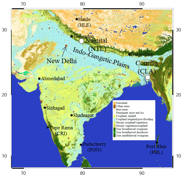
Figure 1 Locations of Nainital (NTL), India (29.36^∘ N, 79.46^∘ E; 1940 m a.s.l.), Comilla (CLA), Bangladesh (23.43^∘ N, 91.18^∘ E; 30 m a.s.l.), and other Indian sites for greenhouse gas (GHG) observation (Bhattacharya et al., 2009; Ganesan et al., 2013; Sharma et al., 2013; Tiwari et al., 2014; Lie et al., 2015; Sreenivas et al., 2016; Chandra et al., 2016) and showing land cover around the South Asia region (Arino et al., 2012).

CLA is located at the Comilla weather station of the Bangladesh Meteorological Department (BMD) (23.43^∘ N, 91.18^∘ E; 30 m a.s.l.) on the edge of a farming village with a flat landscape in central Bangladesh. The surrounding areas of CLA cover the paddy fields and a few farmhouses. The land use in the central Bangladesh region is almost exclusively agricultural land, with the structure of farms developing along the roads. Farmers in this region often burn the biomass (e.g. harvest residuals, firewood, and dung), and it was expected that CO₂, CH₄, CO, H₂, and N₂O were emitted by the burning. Wind and precipitation are strongly influenced by monsoon, and sometimes cyclone hits this region. Wind speeds around the CLA are not very slow on average, e.g., 2–5m s⁻¹. Therefore, we judged that this site can mainly capture the typical greenhouse gas emission and sink effects in central Bangladesh, which is located in the eastern Indo-Gangetic Plain, despite it partly capturing some effects from nearby emissions.

2.2 Air sampling

Flask samples were collected from September 2006 in NTL and from June 2012 in CLA. Inlets were mounted at 7 m above ground level (on the roof of the second floor of the station) in NTL and 8 m above ground level (on top of the 5 m tower on the roof of the one-storey weather station building) in CLA. The height of the inlet of NTL is 5–20 m higher than the height of the canopy close to the inlet. Air samples were collected once a week (usually on Wednesdays) at 14:00 LT into a 1.5 L Pyrex flask with two stopcocks sealed with Viton O-rings via a sampling line (Fig. 2a). The sampling line contained a diaphragm pump (MOA-P108-HB, GAST Co., Ltd.) and a freezer (VA-120, Taitec Co., Ltd.) for dehumidification by a glass trap. The sampling flow rate was approximately 2 L min⁻¹, and the sample was passed through a −30 ^∘C cooler and pressurized to 0.25 MPa after 10 min flushing through the sampling tube and flask. The sampled flasks were packed in a cardboard box and transported to the laboratory of the Center for Global Environmental Research (CGER), National Institute for Environmental Studies, Japan (NIES) (transportation period: 3–7 d), for analyses.

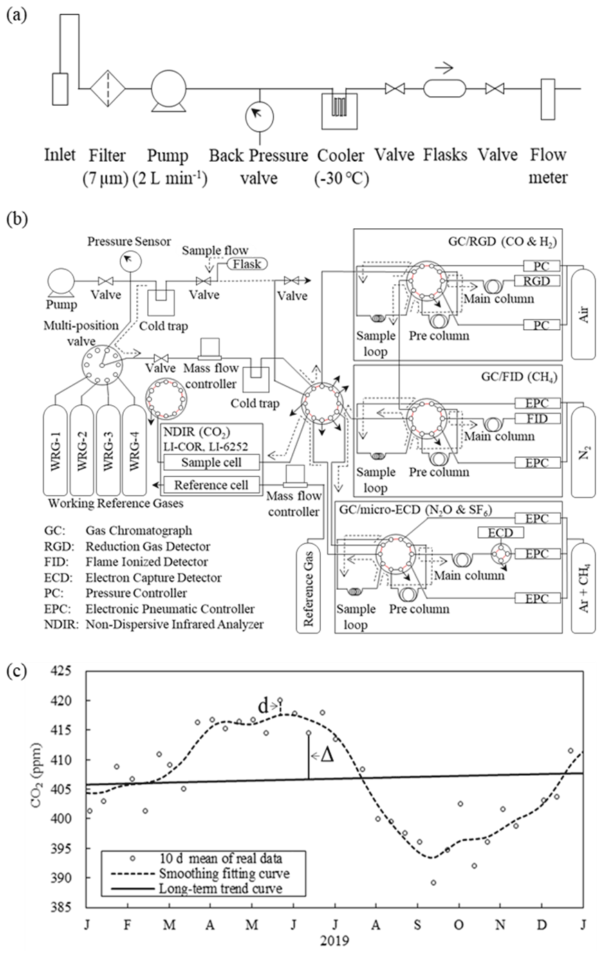
Figure 2 The line used for (a) flask sampling, (b) schematic of measurements of the dry-air mole fraction in the laboratory, and (c) diagram of the calculation method for the “Δ” term (e.g., ΔCO₂), which was calculated by subtraction of the long-term trend curve from the 10 d mean of real data and the “d” term (e.g., dCO₂), which was characterized by the deviation of the 10 d mean of real data from the smoothing fitting curve.

2.3 Measurement methods

An air sample was passed through a −80 ^∘C cold trap for dehumidification and was delivered to each instrument with a flow rate of 40 mL min⁻¹ (see the analysis line in Fig. 2b). A nondispersive infrared analyzer (NDIR; LI-COR, LI-6252) was used for CO₂ analysis, a gas chromatograph equipped with a flame ionization detector (GC-FID; Agilent Technologies, HP-5890 or HP-7890) was used to analyze CH₄, a gas chromatograph with a reduction gas detector (GC-RGD; Agilent Technologies, HP-5890+Trace Analytical RGD-2 or Peak Laboratories, Peak Performer 1 RCP) was used for CO and H₂ analyses, and a gas chromatograph with an electron capture detector (GC-ECD) until 2011 and with a micro-electron capture detector (GC-micro-ECD) from 2012 (Agilent Technologies, HP-6890) were used to analyze N₂O and SF₆.

The sample was injected into the analytical system three times per one flask, and the working standard gases were analyzed after every two flasks. Dry-air mole fractions were measured against each of their working standard gases, which were calibrated with NIES secondary standard gas series (CO₂-NIES09 scale, CH₄-NIES94 scale, CO-NIES09 scale, H₂-NIES96 scale, N₂O-NIES01 scale, and SF₆-NIES01 scale). Comparison between those scales and the National Oceanic and Atmospheric Administration (NOAA) scale in the sixth Round Robin intercomparison (NOAA/ESRL, 2019a) showed −0.04 to −0.09 ppm for CO₂, 3.7 to 4.1 ppb for CH₄, 4.0 to 4.4 ppb for CO, −0.61 to −0.69 ppb for N₂O, and −0.03 to −0.06 ppt for SF₆. We evaluated that the NIES scales were almost the same as NOAA scales except for CH₄, which showed a bias that was beyond the measurement precision of our instrument.

The mole fractions of the respective working standard gases are 379.00, 403.01, 423.84, and 441.10 ppm for CO₂, 1681.50, 1852.12, 1998.83, and 2167.63 ppb for CH₄, 59.84, 164.57, 267.33, and 373.54 ppb for CO, 401.40, 502.98, 610.49, and 715.95 ppb for H₂, 319.23, 326.91, 337.53, and 345.54 ppb for N₂O, and 4.65, 9.77, 14.53, and 19.08 ppt for SF₆. The analytical precision for the repetitive measurements is less than 0.03 ppm for CO₂, 1.7 ppb for CH₄, 0.3 ppb for CO, 3.1 ppb for H₂, 0.3 ppb for N₂O, and 0.3 ppt for SF₆ (Machida et al., 2008).

After the mole fraction analysis, we used the remaining air inside the flask for analysis of δ¹³C-CO₂ and δ¹⁸O-CO₂. The air was introduced into two traps sequentially (−100 and −197 ^∘C), which trapped H₂O and CO₂, respectively. Finally, CO₂ was sealed in a glass tube. Air δ¹³C-CO₂ and δ¹⁸O-CO₂ were measured by MT-252 using the working standard CO₂ gas which was prepared in our laboratory. The method for producing the working standard gas is similar to the method for producing the NIES Atmospheric Reference CO₂ for Isotopic Studies (NARCIS), which is used for interlaboratory-scale comparison (Mukai, 2001). The working standard scales of δ¹³C-CO₂ and δ¹⁸O-CO₂ are the same as those of NARCIS, which were measured by various institutions related to the World Meteorological Organization (WMO) (Mukai, 2003). The differences between NIES scales and INSTAAR (Institute of Arctic and Alpine Research) scales were 0.013 ‰–0.039 ‰ in the mean value range of −8.683 ‰ to −8.759 ‰ for δ¹³C-CO₂ and −0.017 ‰–0.022 ‰ in the mean value range of −1.956 ‰ to −9.299 ‰ of δ¹⁸O-CO₂ in the 6th Round Robin intercomparison (NOAA/ESRL, 2019a). The δ¹⁸O-CO₂ for atmospheric CO₂ in this study is expressed against the value of CO₂ evolved from VPDB calcite (i.e., VPDB-CO₂ scale, IAEA, 1993; Brand et al., 2010). Although the Vienna Standard Mean Ocean Water (VSMOW) scale is often used for δ¹⁸O values of water, CO₂ evolved from VPDB calcite (VPDB-CO₂ scale) has similar δ¹⁸O values of CO₂ equilibrated with VSMOW, which is the reference gas of the VSMOW scale. The difference between them is only 0.263 ‰ (IAEA, 1993; Kim et al., 2015). Additionally, corrections for N₂O bias and δ¹⁷O-CO₂ shown by Brand et al. (2010) were made to obtain final isotope ratios.

2.4 Reference dataset

For comparison with the data of NTL and CLA, we obtained weekly data (CO₂, CH₄, CO, N₂O, SF₆, δ¹³C-CO₂, and δ¹⁸O-CO₂) from the Mauna Loa Observatory (MLO) (19.54^∘ N, 155.58^∘ W; 3397 m a.s.l.) on the NOAA/ESRL website (NOAA/ESRL, 2019b). We also used biweekly data for CO₂, CH₄, CO, H₂, N₂O, and δ¹³C-CO₂ from CRI (15.08^∘ N, 73.83^∘ W; 60 m a.s.l.) on the website of the World Data Centre for Greenhouse Gases (WDCGG) (WDCGG, 2017). The trends of mole fractions of CO₂, CH₄, CO, H₂, N₂O, and SF₆ and the isotopic ratio of δ¹³C-CO₂ and δ¹⁸O-CO₂ were calculated according to the method of Thoning et al. (1989), with a cut-off frequency of 667 d (0.5472 cycles yr⁻¹) for a fast Fourier transform (FFT) filter. We also obtained the DMI and ENSO index from the NOAA/ESRL website (NOAA/ESRL, 2021a, b).

2.5 Weather data

Monthly precipitation data for Nainital use the monthly precipitation of the state of Uttarakhand, which includes Nainital. The data during January 2007 to December 2019 were taken from the rainfall report on the IMD (India Meteorological Department) website (available at: http://hydro.imd.gov.in/hydrometweb/(S(fqu5hsvtq3sitn45rjia4qma))/landing.aspx, last access: 1 September 2021). Monthly precipitation data for Comilla use the average monthly precipitation of the eastern Indo-Gangetic Plain in Bangladesh (Dhaka (23.77^∘ N, 90.38^∘ E and 8 m a.s.l.), Rangpur (25.73^∘ N, 89.23^∘ E and 33 m a.s.l.), Sylhet (24.90^∘ N, 91.88^∘ E and 34 m a.s.l.), Bogra (24.84^∘ N, 89.37^∘ E and 18 m a.s.l.), Ishurdi (24.13^∘ N, 89.05^∘ E and 13 m a.s.l.), Jessore (23.18^∘ N, 89.17^∘ E and 6 m a.s.l.), Feni (23.03^∘ N, 91.42^∘ E and 6 m a.s.l.), Barisal (22.75^∘ N, 90.37^∘ E and 3 m a.s.l.), Chattoogram (22.27^∘ N, 91.82^∘ E and 4 m a.s.l.), and Cox's Bazar (21.43^∘ N, 91.93^∘ E and 2 m a.s.l.)). Data during January 2012 to July 2021 were taken from the JMA (Japan Meteorological Agency) website (available at: http://www.data.jma.go.jp/gmd/cpd/monitor/climatview/frame.php?y=2019&m=7&d=30&e=0, last access: 1 September 2021).

2.6 Back-trajectory analysis

To determine the sources of regional air masses affecting the stations (NTL and CLA), we calculated backward air trajectories using the Meteorological Data Explorer (METEX) system (Zeng and Fujinuma, 2004) available via the website of the Center for Global Environmental Research, National Institute for Environmental Studies (available at: http://db.cger.nies.go.jp/metex/index.html, last access: 1 September 2021). METEX uses three-dimensional wind speed (horizontal and vertical wind) estimated from the European Centre for Medium-Range Weather Forecast (ECMWF) analyses on a 0.5^∘ × 0.5^∘ mesh to calculate 72 h trajectories. We use 1940 m for NTL and 30 m for CLA as the starting heights. We referred to the altitude data when we evaluated the effects of GHG emissions sources near the surface.

The ratio of air mass from the south per year was calculated by the frequency of the air mass from the southern side of the Indian Ocean on the flask sampling date in each year with reference to the 72 h backward air trajectory data calculated by METEX.

2.7 Data analysis method for the short term and long term

Mean values for every 10 d were calculated from the weekly data and were used to calculate the long-term trend and smoothing fitting curve. Because the sampling interval is not punctual and we sometimes had missing data, we decided to use the 10 d average to calculate the trend curve. The value of the missing period was supplemented with an interpolated value from the previous and following data of the missing period for calculating the continuous long-term trend and smoothing fitting curve.

Long-term trends of the mole fractions were calculated based on the idea of Thoning et al. (1989) with a cut-off frequency of 667 d (0.5472 cycles yr⁻¹) for a FFT filter. The smoothing fitting curve was made for a FFT filter with a cut-off frequency of 50 d (7.3 cycles yr⁻¹).

We defined and expressed the seasonal component by a “Δ” term (e.g., ΔCO₂) which was calculated by subtraction of the long-term trend curve from a 10 d mean of real data. Also, we defined and expressed short-term variations by a “d” term (e.g., dCO₂), which were characterized by the deviation of a 10 d mean of real data from the smoothing fitting curve. Figure 2c shows how such components were calculated. Growth rates of mole fractions of observed gases were calculated using the long-term trends.

3 Results and discussion

3.1 Overview of GHG mole fractions at both sites

Basically, the air masses over the Indian subcontinent were transported from the Indian Ocean region during summer (monsoon season) and from the inland during winter. Air mass trajectories are shown for our sampling sites and related sites in Fig. 3. In the case of anthropogenic GHGs, except CO₂, their mole fractions at CLA generally showed relatively low values when the air mass came from the ocean, while the mole fractions were relatively high when the air mass came from inland. On the other hand, mole fractions of GHGs at NTL overall did not show relatively low values even if the air mass came from the Indian Ocean region (i.e., southeasterly wind) because the air mass from the Indian Ocean was strongly affected by local GHG emissions while passing over the Indo-Gangetic Plain. However, the CO₂ mole fraction changed not only due to transport, but also due to the photosynthetic sink strength of terrestrial ecosystems and cultivated crops.

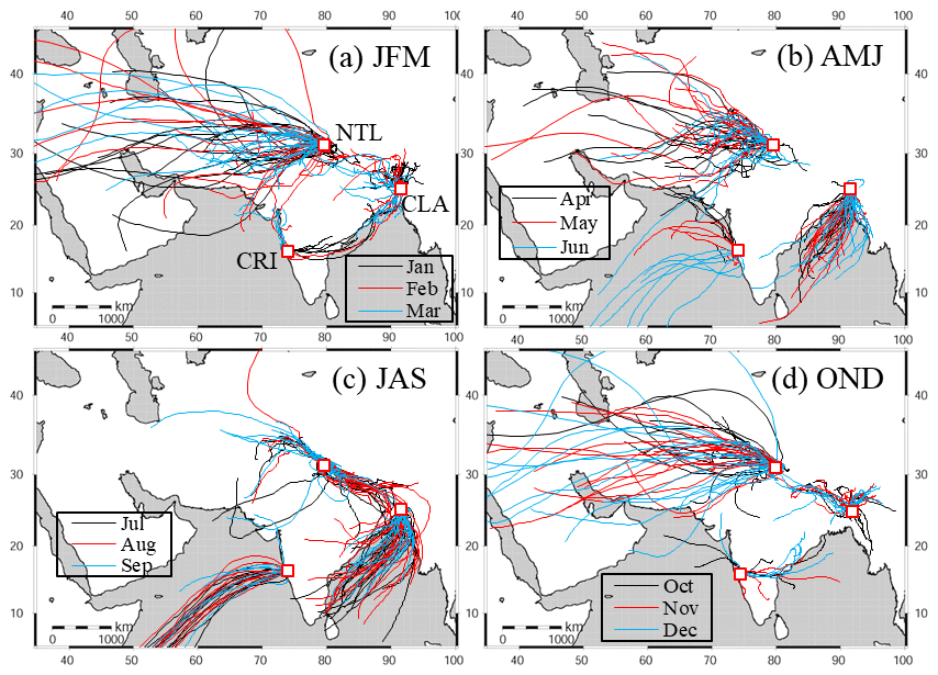
Figure 3 72 h back-trajectory of NTL, CLA, and CRI in (a) January–March (JFM), (b) April–June (AMJ), (c) July–September (JAS), and (d) October–December; 72 h back-trajectory at NTL and CLA shown for 2012–2016 and the back-trajectory at CRI shown for 2009–2013.

Annual mean GHG mole fractions at NTL and CLA are summarized in Table 1. Annual CO₂ mole fractions at both sites were quite low compared to MLO and other Indian sites such as CRI. For example, in 2010, 386.5 ppm was reported at NTL, 391.9 ppm at CRI (Bhattacharya et al., 2009), and 391.3 ppm at PON (Lin et al., 2015). Note that there are no data for CLA in 2010; however, the annual CO₂ mole fraction at CLA is usually only 1–2 ppm higher than at NTL. This seemed to be due to the influence of photosynthesis at both sites. Generally, the CO₂ mole fractions at NTL and CLA decreased strongly (typically twice a year) due to photosynthesis of local crops, making the annual CO₂ mole fractions lower than at other sites despite the likelihood that anthropogenic emissions are high in this area.

Table 1 Annual mean atmospheric mole fractions of CO₂, CH₄, CO, H₂, N₂O, and SF₆, isotopic ratios of δ¹³C-CO₂ and δ¹⁸O-CO₂, and CO₂ growth rates at Nainital (NTL) and Comilla (CLA) in 2007–2020.

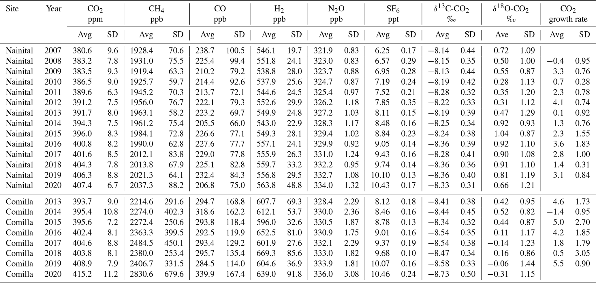
On the other hand, the annual mean mole fractions of CH₄, CO, H₂, and N₂O at NTL and CLA (Table 1) were almost at the highest levels on the Indian subcontinent due to the influence of strong emission sources. For example, the annual mole fractions of NTL and CLA were 50–470 ppb for CH₄, 30–200 ppb for CO, and 0–5 ppb for N₂O higher compared to other Indian sites (e.g., CRI, Bhattacharya et al., 2009; HLE, PON, and PBL, Lin et al., 2015). In this region, high CH₄ and N₂O emissions were possible from paddy fields and cultivated areas. Also, much CO is considered to be produced by biomass burning in this region. As for H₂, the mole fraction at CLA was higher than those at other Indian sites; however, it was relatively low at NTL compared to other sites such as CRI (Bhattacharya et al., 2009), PON, and PBL (Lin et al., 2015) but similar to HLE, which is located on a higher mountain. In the case of the SF₆ mole fraction, it has smaller regional differences, suggesting there are no remarkable SF₆ sources near the measurement sites. Below we describe in detail the characteristics of sources and sinks of each component (CO₂, δ¹³C-CO₂, δ¹⁸O-CO₂ CH₄, CO, H₂, N₂O, and SF₆) at NTL and CLA on the Indo-Gangetic Plain in terms of seasonal variations, amplitudes, and growth rates.

3.2 CO₂ and δ¹³C-CO₂

3.2.1 CO₂ mole fraction and growth rate variations

Figure 4 shows the time series of the atmospheric CO₂ mole fraction and the isotopic ratio of δ¹³C-CO₂ at our sampling sites (NTL and CLA) together with data from CRI on the western coast of India and MLO in Hawaii. The CO₂ mole fractions at NTL and CLA in August–October were characteristically lower (approximately 10–20 ppm) than the mole fractions observed at CRI and MLO. The CRI and MLO sites are representative of CO₂ mole fractions in the Southern Hemisphere and Northern Hemisphere, respectively, for the period of the southwestern monsoon season (June–September). On the other hand, the δ¹³C-CO₂ at NTL and CLA was inversely correlated with the CO₂ mole fractions, and generally the values at both sites were higher than at MLO and CRI.

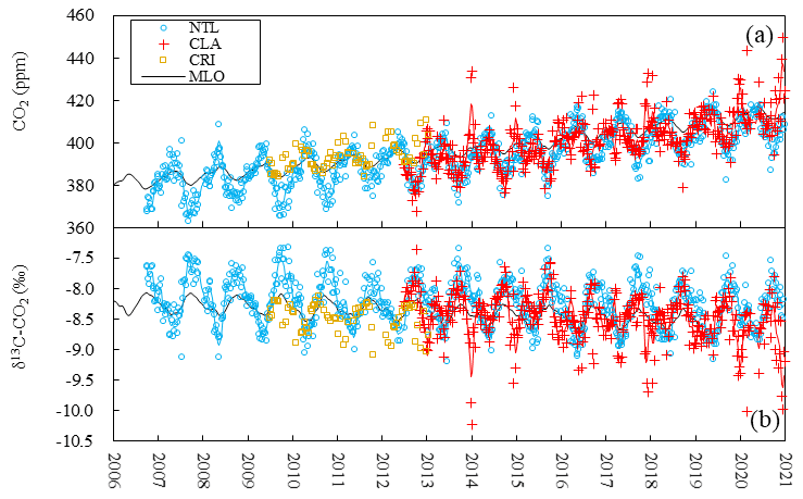
Figure 4 Time series of the (a) atmospheric CO₂ mole fraction and the (b) isotope ratio of δ¹³C-CO₂ at NTL, CLA, CRI, and MLO in 2006–2020.

Air masses at NTL and CLA in August–October passed over the Indo-Gangetic Plain and the southeastern area of India, respectively, while the air masses of CRI were transported from the Indian Ocean region (Fig. 3). Thus, it was suggested that the air mass from the Indian Ocean in August–October prevailing over CRI was hardly influenced by anthropogenic emission and photosynthesis over the Indian subcontinent, whereas CO₂ mole fractions over NTL and CLA seemed to be influenced during these seasons by the sources and sinks on the Indo-Gangetic Plain and the southern/eastern areas of the Indian subcontinent. Such transport characteristics must affect the annual average and growth rates in the CO₂ molar ratio and δ¹³C-CO₂ in addition to their seasonal variations.

We show the CO₂ growth rates observed at NTL, CLA, and MLO in Fig. 5a. Mean CO₂ growth rates at NTL (approximately 2.1 ppm  yr⁻¹ during 2007–2020) and CLA (approximately 2.9 ppm yr⁻¹ during 2013–2020) were similar to other sites (e.g., MLO). However, variations of the calculated growth rates were greater than those at MLO. The range was 0–5 ppm yr⁻¹ in the case of NTL, and CLA had higher variability than NTL because local sink and source influences affected the concentration more than remote sites such as MLO. In general, Pacific sites such as MLO and Japanese remote sites in the Northern Hemisphere showed a relationship between CO₂ growth rates and the ENSO index (e.g., Keeling, 1998). This relationship is often explained from the viewpoint of a global temperature anomaly, which has a strong relationship with the ENSO index. On the other hand, the variability at NTL has no associations with the variability in the CO₂ growth rate at MLO and the ENSO index (Fig. 5b). Both growth rates seemed to be slightly inversely correlated with each other from 2007 to 2015. However, since then, similar relatively high growth rates have been observed for both sites around 2015–2016 and 2018–2019, indicating that, overall, the CO₂ growth rate at NTL is less correlated with the CO₂ growth rate at MLO and the ENSO index.

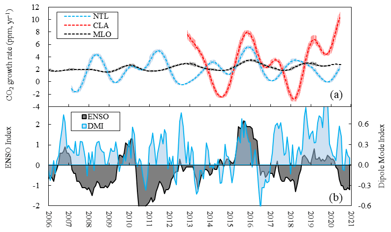
Figure 5 (a) Growth rates of the CO₂ mole fraction at NTL, CLA, and MLO in 2006–2020 and (b) the El Niño–Southern Oscillation (ENSO) index in 2006–2020 and the Dipole Mode Index (DMI) in 2006–2020.

It is well known that the Indian Ocean Dipole controls meteorological conditions such as air mass transportation and precipitation patterns on the Indian subcontinent (e.g., Saji et al., 1999; Ashok et al., 2004; Hong et al., 2008). Such changes in regional climatic pattern could affect the CO₂ uptake flux by plants in the surrounding area and the atmospheric movement, leading to a change in the CO₂ growth rate. However, we did not find a simple relationship between DMI and CO₂ growth rate at NTL (Fig. 5b). Here we have shown that the pattern of CO₂ growth rate in this region is different from the global pattern seen in places like MLO, but the relationship between local climatic factors and changes in CO₂ sinks and emissions is likely to be complex, and further study is needed to interpret the differences.

3.2.2 Seasonal variation and its characteristics

Figure 6a–d show the seasonal variations in CO₂ mole fractions and isotopic ratios of δ¹³C-CO₂ at NTL, CLA, CRI, and MLO, which were calculated by subtraction of the measured value from the long-term trend. The annual amplitudes of the CO₂ mole fraction (Table 2) at NTL (22.1 ± 3.9 ppm) and CLA (20.3 ± 5.7 ppm) were much larger than those at other Indian sites (CRI, 15 ppm; HLE, 8.2 ppm; PON, 7.6 ppm; PBL, 11.1 ppm). Also, the annual amplitudes of δ¹³C-CO₂ at NTL (0.96 ‰± 0.16 ‰) and CLA (0.85 ‰± 0.19 ‰) were larger than that at CRI (approximately 0.6 ‰). These results suggested that the atmospheric CO₂ mole fractions of NTL and CLA were strongly influenced by photosynthesis of local plants in summer and their respiration in winter and other anthropogenic emissions which were moderated at the other sites by the influence of the oceanic air. Also, small episodic peaks of the atmospheric CO₂ mole fraction and isotopic ratio of δ¹³C-CO₂ of CLA at the beginning of each year were influenced by the biomass burning for heating in the close region, which is considered to be the inland area from the site according to the air trajectory analysis.

Table 2 Mean annual amplitudes of seasonal variation in atmospheric mole fractions of CO₂, CH₄, CO, H₂, N₂O, and SF₆ and δ¹³C-CO₂ and δ¹⁸O-CO₂ at NTL during 2007–2020 and at CLA during 2013–2020.

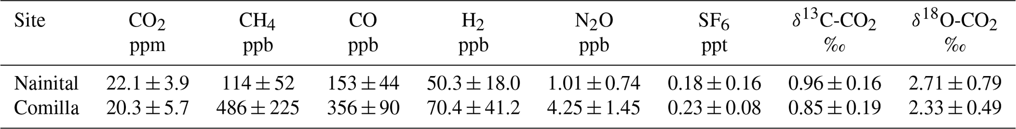
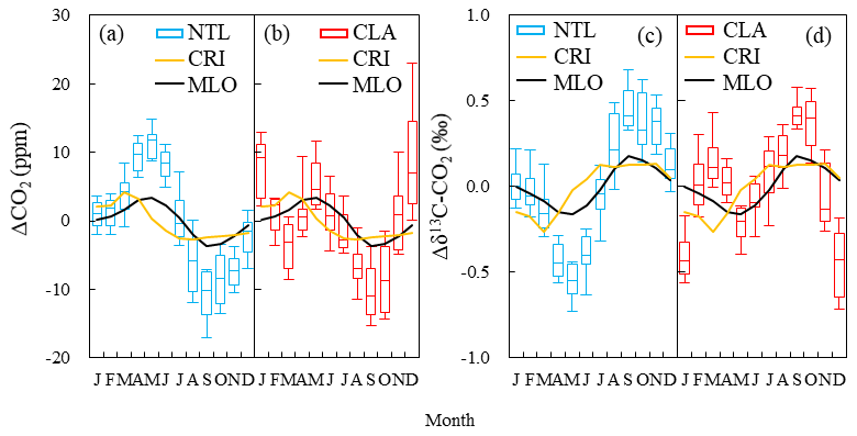
Figure 6 Seasonal variations in the CO₂ mole fraction at (a) NTL and (b) CLA and the isotope ratio of δ¹³C-CO₂ at (c) NTL and (d) CLA. Boxes with blue and red are for Nainital and Comilla, and the black and yellow lines are for MLO and CRI, respectively. Median values (the line in the box) and the inner 50th percentile of the value (box) and inner 90th percentile of the value are from the monthly averaged CO₂ mole fractions.

As shown in Figs. 4a and b and 6b and d, the seasonal variation pattern at CLA has two lower seasons in CO₂ and two higher seasons in δ¹³C-CO₂ in February–April and July–October. Similarly, in the case of NTL, we sometimes observed relatively low mole fractions of CO₂ in February–March and September and higher δ¹³C-CO₂. In general, in many cases, including at MLO, only a summer minimum CO₂ mole fraction is observed, while a minimum in February–March is not usually observed.

Twice-yearly decreases in the CO₂ mole fraction have also been observed at several Indian sites such as Dehradun (northern Indian site; Sharma et al., 2013), Sinhagad (western Ghats site; Tiwari et al., 2014), Ahmedabad (western Indian site; Chandra et al., 2016), Shadnagar (central Indian site; Sreenivas et al., 2016), and PON (southeastern coastal Indian site; Lin et al., 2015); however, these studies did not clearly mention such variations. Umezawa et al. (2016) reported that the decrease in the CO₂ mole fraction near the ground in February–March was caused by photosynthesis of local crops, which was detected by the vertical CO₂ profiles over New Delhi Airport. Those sites are located on the Indo-Gangetic Plain or received air masses passing over the Indo-Gangetic Plain or Indian subcontinent. On the other hand, the decrease in the CO₂ mole fraction in February–March was not detected at CRI (western coastal Indian site; Bhattacharya et al., 2009), HLE (northwestern Himalayan site), or PBL (Andaman Islands site) (Lin et al., 2015). These sites are not located on the Indo-Gangetic Plain. Thus, air masses at these sites must be mainly transported from the ocean or from areas other than the Indian subcontinent during these periods.

The characteristic CO₂ seasonal variation on the Indo-Gangetic Plain (including NTL and CLA) is very likely to be related to CO₂ uptake by regional vegetation. Generally, in the case of the state of Uttar Pradesh located in the center of the Indo-Gangetic Plain, rice and other summer plants (maize, millets, etc.) are planted mainly in June–July and harvested in October–November, while large areas of wheat are sown in October–December and harvested in March–April. Therefore, relatively low CO₂ mole fractions observed in those periods are considered to be due to CO₂ uptake by plants cultivated in each season near NTL.

In Bangladesh, rice, being the staple food, is cultivated three times a year in some regions. Usually rice is grown twice (aus and amon rice) from April to October (including the monsoon season); however, rice is also often cultivated (boro rice) in the winter season from November to April (SID/MP, 2018). Other agricultural products include maize, jute, and vegetables in the summer season and a small amount of wheat in the winter season. Therefore, we concluded that the observed lower CO₂ mole fractions in July–October and February–March were influenced by CO₂ uptake by local plants (mainly rice). Especially at CLA, the lower mole fraction in February–March was clear, and a strong contribution from CO₂ uptake from boro rice was estimated. As another viewpoint on CO₂ seasonal variation, we observed that the CO₂ maximum in May was not so high, while the CO₂ mole fraction in December was higher. Because precipitation in Bangladesh is stronger than in the northern Indian region, the duration of rice cultivation over summertime is also longer than in northern India. Therefore, the contribution of plant uptake to the CO₂ mole fraction in the atmosphere at CLA over the summer season is likely to be relatively large compared to that at NTL.

Thus, the decreases in the CO₂ mole fractions in February–March and September in NTL and CLA were estimated to be caused by photosynthesis of plants cultivated in each season over the Indo-Gangetic Plain. NTL and CLA indicated this more clearly compared with other Indian sites due to the proximity to the source region. Figure 7a shows the relationships between the annual mean CO₂ mole fraction and δ¹³C-CO₂ in 2010 and 2012. The slope between the CO₂ mole fraction and δ¹³C-CO₂ showed −0.050 and −0.054 ‰ ppm⁻¹, which indicated that the spatial variability of the atmospheric CO₂ mole fraction (e.g., a lower mole fraction at NTL than at MLO and CRI) basically occurred due to CO₂ exchange between the atmosphere and terrestrial biosphere.

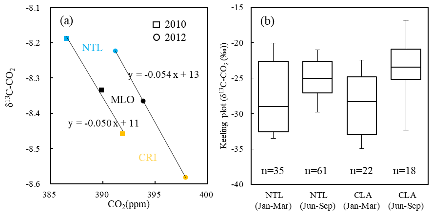
Figure 7 (a) Relationship between the annual values of the CO₂ mole fraction and isotopic ratio of δ¹³C-CO₂ at NTL, CRI, and MLO in 2010 and 2012 and (b) the intercept values of the Keeling plot of NTL and CLA in January–March and June–September.

Furthermore, we examined the relationship of the CO₂ mole fraction and carbon isotope ratio, because there are some seasonal differences in the species cultivation. On the Indo-Gangetic Plain, rice (especially in Bangladesh) and wheat (especially in northern India), as C₃ plants, are cultivated in January–March, while C₄ plants, e.g., maize, sugarcane, sorghum, and bajra (pearl millet), in addition to rice are cultivated on the Indo-Gangetic Plain and in Bangladesh in June–September (DAC/MA, 2015; SID/MP, 2018; DES/MAFW, 2019). We calculated the end-member of the isotope value for absorbed CO₂ by using intercept values of the Keeling plot between the reciprocal of the CO₂ mole fraction and the ratio of δ¹³C-CO₂ obtained from two continuous datasets of air samples, which has >1 ppm difference in CO₂ mole fraction and >0.05 ‰ in δ¹³C-CO₂. Since in this study two datasets had 1-week intervals, we assumed that the difference in CO₂ and δ¹³C between two datasets would include broader influences of photosynthetic activities from relatively large areas on the Indo-Gangetic Plain.

We found that the intercept values of NTL and CLA showed differences in January–March and June–September (Fig. 7b), which appeared to reflect the differences in the contributions of C₃ and C₄ plants in this region. In June–September, we found relatively heavier intercept values at both NTL (−25.0 ‰ ± 2.4 ‰) and CLA (−23.5 ‰ ± 4.1 ‰), suggesting that C₄ plants partly contributed to the CO₂ absorption (or emission) in this season, while in January–March, the end-member showed −29.0 ‰ ± 4.3 ‰ (NTL) and −28.3 ‰ ± 4.0 ‰ (CLA), which were similar to the general C₃ plant (rice or wheat). If we assume the value for the C₄ plant to be −12 ‰ to −14 ‰, the contributions of the C₄ plant in NTL and CLA were approximately 25 % ± 5 % and 31 % ± 9 %, respectively. According to the database (DAC/MA, 2015; SID/MP, 2018; DES/MAFW, 2019) for crop area in Uttar Pradesh, the area's ratio of C₄ plants (e.g., maize and sugarcane) to C₃ plants in the summer season was approximately 26 % in 2012, which was a similar proportion to that estimated by the C isotope ratio. In the case of Bangladesh, despite there being no recent data reported, according to data in 2008, the area for maize was approximately <10 % compared to the rice area. However, based on the recent C isotope ratio, it appears likely that more maize has been cultivated.

3.3 δ¹⁸O-CO₂

In general, δ¹⁸O-CO₂ is related to that value of water in plants and soil, because oxygen atoms of CO₂ can be exchanged with oxygen atoms of H₂O in plant and bacteria cells during photosynthesis and soil respiration. Plants and soil water mainly originate from rainwater in the study region; however, in the case of the agricultural area, water is often introduced by irrigation systems using river water and groundwater. In many cases, photosynthesis produced relatively heavier δ¹⁸O-CO₂ than soil respiration because δ¹⁸O-H₂O in plants becomes heavier than soil water due to plant transpiration.

Larger amplitudes (approximately 3 ‰) in the seasonal variation of δ¹⁸O-CO₂ at both NTL and CLA were observed compared to that of MLO (approximately 0.4 ‰) (Fig. 8a). The isotopic ratio of δ¹⁸O-CO₂ at CRI (Bhattacharya et al., 2009) was reported to have similar seasonal variation (i.e., high in winter (November–February) and low in September) to our sites. In the Pacific sites like MLO, δ¹⁸O-CO₂ has a maximum peak from spring to summer, when photosynthesis activity becomes dominant, while a minimum is seen around fall, when the contribution of soil respiration exceeds that of photosynthesis. On the other hand, Indian subcontinent sites seemed to have fairly different seasonal variation patterns, with a maximum in January–February, gradually decreasing from March to September/October and subsequently rapidly increasing (Fig. 8c and d). Such seasonal variation may be influenced by photosynthesis and soil respiration in these regions. However, because many crops are cultivated through the year in these areas (as mentioned in Sect. 3.2), the contribution of photosynthesis to the seasonal variation may be relatively small. High soil respiration activity in the wet season can contribute a little more than during the dry season.

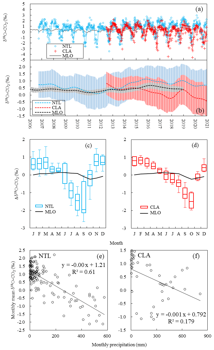
Figure 8 Time series of (a) measured values and (b) the long-term trend for the isotopic ratio of δ¹⁸O-CO₂ at NTL, CLA, and MLO in 2006–2020, the seasonal variation of δ¹⁸O-CO₂ at (c) NTL and (d) CLA, and the relationship between monthly precipitation of the state of Uttarakhand and Bangladesh and the monthly mean of δ¹⁸O-CO₂ at (e) NTL and (f) CLA.

On the other hand, seasonal variations in δ¹⁸O of rainwater itself seemed to affect δ¹⁸O-CO₂ through photosynthesis and respiration processes. For example, Sengupta and Sarkar (2006) showed that the δ¹⁸O-H₂O in rain at New Delhi (western Indo-Gangetic Plain) had a higher value in March–May and a minimum value in September. Such variation was fairly consistent with the seasonal variation in δ¹⁸O of CO₂ at NTL. Similarly, CLA has a minimum δ¹⁸O-CO₂ in the atmosphere in October, which was the same month in which the minimum δ¹⁸O-H₂O was observed in rain in eastern Indo-Gangetic Plain areas (e.g., Kolkata near Bangladesh, Sengupta and Sarkar, 2006; Cherrapunij, eastern Indo-Gangetic Plain; Breitenbach et al., 2010). During the rainy season, due to the so-called “amount effect”, δ¹⁸O-H₂O in rain will decrease with an increase in the amount of precipitation (e.g., Rozanski et al., 1993). However, in the Indian region it has been reported that seasonal changes in the origin of moisture strongly affected the δ¹⁸O-H₂O (Sengupta and Sarkar, 2006; Tanoue et al., 2018). In winter (i.e., when there is less rain), moisture comes from the west or north. Therefore, the northern area of the Arabian Sea and the western land area supply moisture, which has a higher δ¹⁸O-H₂O. However, the air mass in the summer monsoon season (mainly June–September) comes from the southern part of the Arabian Sea and sometimes passes over the Bay of Bengal, carrying much moisture. The value of δ¹⁸O-H₂O in the moisture in the air mass decreases with the process of raining along the air trajectory. In the post-monsoon season (mainly October–December), some portion of moisture comes from the Pacific, Bay of Bengal, and inland area (Tanoue et al., 2018).

In the winter monsoon season (mainly February–May), δ¹⁸O-H₂O in rain was reported to be approximately 0 ‰–1 ‰ (vs. VSMOW). During the winter monsoon season, there is little precipitation, so plant cultivation utilizes irrigation systems using river water and groundwater. River water and groundwater usually show not so large seasonal variation in δ¹⁸O and have a value close to the annual mean of δ¹⁸O-H₂O in rain, such as −6 ‰ to −8 ‰ (Kumar et al., 2019). According to the variation of δ¹⁸O-CO₂, in winter its value was approximately 2 ‰ (vs. VPDB-CO₂; the VPDB-CO₂ scale is fairly close to the scale of CO₂ equilibrated with VSMOW, as mentioned in Sect. 2.3), which was higher than that of rain and other water reservoirs, suggesting that δ¹⁸O-H₂O in plants and soil must become higher due to transpiration during dry and relatively warm conditions in winter.

Based on the fact that, during the summer monsoon season, δ¹⁸O-CO₂ decreased from 1 ‰ to −2 ‰ with a decrease in δ¹⁸O-H₂O from 0 ‰ to −10 ‰ or −15 ‰ in the rain, the range of variation in δ¹⁸O-CO₂ was approximately one-third or one-fifth that of rain. Because land water may come from both rain and irrigation systems, the real ranges of δ¹⁸O in soil water and plant water are likely to be smaller than in the case of rain only. Furthermore, because CO₂ from soil respiration contributes more in the rainy season, a balance between photosynthesis and respiration CO₂ will, in general, have a small effect on the seasonal variation.

As for the annual trend of δ¹⁸O-CO₂ shown in Fig. 8b, NTL showed a similar pattern to that of MLO, whereas CLA showed a different trend. The δ¹⁸O-CO₂ at NTL began at 0.8 ‰ in 2007, decreased to 0.2 ‰ in 2011, and then again became heavier (toward 1.0 ‰) during 2014–2016 (Fig. 8b). In northern India, relatively high precipitation was reported during 2011–2013. The tendency of lower δ¹⁸O-CO₂ may have some relationship with the amount of precipitation. In 2008 and 2016 considerable amounts of precipitation fell near NTL. The δ¹⁸O-CO₂ level also seemed to become relatively low. A La Niña event occurred from late 2010 to 2012, and the amount of precipitation increased worldwide from 2010 to 2013. Such large-scale climatic effects are very likely to affect the δ¹⁸O-CO₂ level observed at MLO. In the case of CLA, precipitation increased in 2015–2017 and 2019–2020 (rather than in 2011–2013), and the δ¹⁸O-CO₂ level at CLA seemed to become lower at that time with the increase in precipitation. Analyzing the relationship between the monthly amount of precipitation and δ¹⁸O-CO₂ in Fig. 8e and f, a weak negative correlation can be seen (if the monthly mean δ¹⁸O-CO₂ at CLA adds 1 or 2 months of time lag to the monthly mean of the precipitation, the correlation coefficient (R²) between the monthly mean δ¹⁸O-CO₂ at CLA and the monthly mean of precipitation increases to be 0.4 or 0.5). Therefore, the amount of precipitation partly contributes to the regional level of δ¹⁸O-CO₂. However, it must be influenced not only by precipitation, but also by seasonal changes in air flow patterns and rain systems, as explained above, as well as by the water reservoir situation, soil water content at that time, and photosynthesis in the region.

If the groundwater storage decreases due to wider usage of irrigation and/or less precipitation in recent times, it causes a stronger transpiration effect in the soil environment, making the δ¹⁸O of soil water heavier than usual. Roxy et al. (2015) and Asoka et al. (2017) reported that precipitation over the Indian subcontinent and groundwater storage in northern India have had a decreasing trend due to Indian Ocean warming, which is estimated to have occurred due to the weakening trend of the summer monsoon cross-equatorial flow (Swapna et al., 2014). However, much longer records of CO₂ isotopic ratios are needed to clarify the increasing trend in δ¹⁸O-CO₂ and the relationship with climatic changes in this region.

3.4 CH₄

The CH₄ mole fractions at NTL and CLA are illustrated in Fig. 9a. We detected high CH₄ mole fractions at NTL and CLA, where they sometimes exceeded 2100 and 4000 ppb, respectively, showing that the Indo-Gangetic Plain region had relatively strong CH₄ emissions. The seasonal amplitude of the CH₄ mole fraction, especially at CLA (486 ± 225 ppb; Table 2), was much larger than those of other Indian sites such as NTL (114 ppb), CRI (200 ppb) (Bhattacharya et al., 2009), Darjeeling (400 ppb) (Ganesan et al., 2013), HLE (29 ppb), PON (124 ppb), and PBL (144 ppb) (Lin et al., 2015), which indicated that the contribution of the CH₄ source (e.g., rice cultivation) around CLA was relatively strong. Mean seasonal variations in the CH₄ mole fraction for both sites were calculated and are shown in Fig. 9c and d. The mole fractions at both NTL and CLA had the highest peak in August–October and a small peak in March. In general, the CH₄ mole fraction in the Northern Hemisphere decreased in July–September (summer season) through the decomposition process by reaction with OH radicals during this period. A higher CH₄ mole fraction in this period strongly suggests that there are some sources of CH₄. Observation results at Darjeeling (northeastern Indian site; Ganesan et al., 2013), HLE (Lin et al., 2015), and Shadnagar (Sreenivas et al., 2016) also indicated high CH₄ mole fractions during August–October. Ganesan et al. (2013) reported that the CH₄ mole fraction at Darjeeling was enhanced by transported air masses from the Indo-Gangetic Plain. Lin et al. (2015) and Sreenivas et al. (2016) showed that the high CH₄ mole fractions at HLE and Shadnagar were influenced by emissions from paddy fields and wetlands. Garg et al. (2011) showed that CH₄ emission from rice fields was estimated to be approximately 17 % of the total CH₄ emissions in India. According to the emission database of EDGAR v4.3.2 (EC-JRC/PBL, 2016), rice cultivation was the largest source of CH₄ (approximately 50 %) in Bangladesh.

Figure 9 Time series of (a) measured values and (b) growth rates of the CH₄ mole fraction at NTL, CLA, CRI, and MLO in 2006–2020, the seasonal variation in the CH₄ mole fraction at (c) NTL and (d) CLA, and the relationship between the short-term components of dCO and dCH₄ at (e) NTL and (f) CLA during January–March (JFM), April–June (AMJ), July–September (JAS), and October–December (OND).

Bhatia et al. (2011) measured the CH₄ flux from paddy fields at New Delhi and showed that it was the highest in August–September due to the increase in the activity of rice roots and bacteria in the paddy field soils. Ali et al. (2012) also measured the CH₄ flux from paddy fields at Bangladesh and reported that the CH₄ flux was maximized within 77–98 d after the planting of rice due to the increase in root respiration and carbon in soil. It was considered that both March and September–October were consistent with the timing of increasing CH₄ production at rice fields according to the customary cultivation schedule of rice in this region. In Bangladesh and the eastern Indian district, rice is cultivated from November to September, as mentioned above in the CO₂ section, and CH₄ emissions are considered to continue during winter, supporting higher CH₄ mole fractions from August to March, especially at CLA.

On the other hand, CRI (Bhattacharya et al., 2009), PON, and PBL (Lin et al., 2015) did not show higher CH₄ mole fractions in August–October, as shown in Fig. 9c and d. The air masses at those sites in August–October were transported from the Indian Ocean, which may have only a minimal influence from agricultural emission.

CH₄ mole fractions at NTL and CLA were higher than that at MLO, even at the time of year when rice is not cultivated. CH₄ emissions from the enteric fermentation and wastewater handling were reported to be large sources according to the emission database in EDGAR v4.3.2 (EC-JRC/PBL, 2016). Garg et al. (2011) reported that enteric fermentation by cattle and buffalo contributes approximately 40 % of emissions in India. Such CH₄ emissions must always elevate the CH₄ mole fraction in the air mass in these sites regardless of the season.

In addition, biomass burning (including residential cooking and agricultural residue burning) is very likely to have a contribution to the CH₄ mole fraction according to the inventory evaluation (i.e., 21 % contribution; Garg et al., 2011). Reasonably good correlations were seen between short-term components in variations of CH₄ and CO in January–March, April–June, and October–December. Ratios of dCH₄ to dCO showed ranges such as 0.64–0.80 ppb ppb⁻¹ in NTL and 1.85–1.98 ppb ppb⁻¹ in CLA, as shown in Fig. 9e and f. One of the major CO sources in India was considered to be biomass burning (Dickerson et al., 2002). Akagi et al. (2011), EC-JRC/PBL (2016), and Sfez et al. (2017) reported that the emission ratios of CH₄ to CO in biomass burning such as crop residue burning, firewood burning, and biogas burning were 0.04–0.90 ppb ppb⁻¹. Therefore, the ratios observed in these seasons could suggest a strong influence on CH₄ and CO emissions from biomass burning (such as crop residue burning), despite the other large CH₄ emissions such as paddy fields and waste treatment, which will increase the ratio, especially at CLA in July–September.

As a result, it is evident that annual CH₄ mole fractions at the sites used in this study on the Indo-Gangetic Plain are enriched by various CH₄ sources, depending on the season. Generally speaking, because April–June is a dry and hot season, CH₄ decomposition processes will proceed, decreasing its mole fraction at both sites.

The variability in the CH₄ growth rate in the trend line at NTL was different to the variability at MLO (Fig. 9b), which may be influenced by regional climatic condition, including the Indian Ocean Dipole. Because the frequency of air mass transportation from the south increased if the Indian Ocean Dipole was often activated, the air mass passed over the Indo-Gangetic Plain (which has strong CH₄ emissions), reaching NTL with a high CH₄ mole fraction. The difference between the variability in the CH₄ growth rate between NTL and CLA may also be explained by the above hypothesis. If the frequency of air mass transportation from the south increased by the activation of the Indian Ocean Dipole (e.g., in 2015) because the air mass was directly transported from the Indian Ocean with a relatively low CH₄ mole fraction, the CH₄ mole fraction at CLA would become relatively low compared to a usual year (Fig. 9b). On the other hand, as mentioned previously, in 2015–2017, even in the high Indian Ocean Dipole Mode, Bangladesh had relatively high precipitation, which could strengthen CH₄ production from rice paddy fields and other aquatic environments. This potential situation matched the high CH₄ mole fraction well in summer and the high growth rate at CLA during 2016–2017.

3.5 CO

High annual CO mole fractions at both NTL and CLA (Table 1) indicated that the atmosphere over the Indo-Gangetic Plain was influenced by strong CO emission sources such as burning of harvest residues and residential burning using solid biofuel, which are considered to be the main CO emission sources in the region (EC-JRC/PBL, 2016). However, of course, CO originating from car exhaust and industrial activities remains very likely to have made some contributions to the CO mole fraction (EC-JRC/PBL, 2016).

The main crops around NTL are rice and wheat, and the harvesting periods are September–November and April–May, respectively (DAC/MA, 2015). Farmers in this area generally burn harvest residues at their farmland after harvest (Lohan et al., 2018). Venkataraman et al. (2006) reported that the amount of burning on the western Indo-Gangetic Plain has two peaks annually, i.e., in May and November. We could observe the same seasonal variation in the CO mole fraction in the atmosphere at NTL (Fig. 10c). Kumar et al. (2011) also reported that the highest densities in fire spots were seen in spring and autumn on the western Indo-Gangetic Plain. These suggested that CO emissions from the burning of harvest residues was one of the most important sources on the western Indo-Gangetic Plain in these seasons.

Figure 10 Time series of (a) measured values and (b) growth rates of CO mole fractions at NTL, CLA, CRI, and MLO in 2006–2020 and the seasonal variation of CO mole fractions at (c) NTL and (d) CLA.

On the other hand, the seasonal variation in CO mole fraction at CLA exhibited only one peak in October–March (Fig. 10d). Such seasonal variation was also detected at CRI (Bhattacharya et al., 2009), PON, PBL (Lin et al., 2015), and Ahmedabad (Chandra et al., 2016). In Bangladesh, after the end of the monsoon (October–March), harvest residues are burnt and used to make bricks using some kinds of biofuel as a heat source (Guttikunda et al., 2013). Also, dung is burnt for the stove (Venkataraman et al., 2010) during the winter season. In addition, biofuel is used for cooking (Lawrence and Lelieveld, 2010) throughout the year. Those activities could emit large amounts of CO (Streets et al., 2003; Venkataraman et al., 2010; Maithel et al., 2012).

In addition, the seasonal amplitude of the CO mole fraction (Table 2) at CLA (356 ± 90 ppb) at the eastern Indo-Gangetic Plain site was much larger than that observed at other Indian sites (e.g., CRI – 200 ppb, PON – 78 ppb, PBL – 144 ppb, and Ahmedabad – 270 ppb). The highest CO amplitude observed at CLA was consistent with the model estimation of CO emissions, which showed that the eastern Indo-Gangetic Plain included areas with the highest CO emissions (Kumar et al., 2013).

On the other hand, the annual mean CO mole fraction at NTL gradually decreased approximately by 50 ppb for 10 years (2006–2015; Fig. 10a). Especially the monthly mean CO mole fraction in November of each year (i.e., the highest level in the year) at NTL decreased by 120 ppb during that period. This suggests that the amount of harvest residues burnt decreased, the ratio of incomplete combustion in car engines was improved, or the type of fossil fuel for cooking changed from biofuel to natural gas. Such decreasing trends in the CO mole fraction level were also detected by Pandey et al. (2017), who reported total-column CO levels during 2003–2014 over the Indo-Gangetic Plain. However, the CO mole fraction level at NTL appeared to increase slightly from 2015. Although the reason for the increase is unclear from this study only, CO emissions from car exhaust were recently estimated to have increased (EC-JRC/PBL, 2016). Therefore, further monitoring is important.

The trend in the CO mole fraction and its interannual variability at NTL was similar to those in CH₄ at NTL (Figs. 9b and 10b). The mole fractions of CO and CH₄ at NTL tended to be slightly higher when the air mass passed over the Indo-Gangetic Plain, where there are strong sources of both CO and CH₄. In 2015 and 2017, a large positive Indian Dipole Mode occurred in addition to El Niño in 2015. Therefore, we observed more frequent southern winds, causing higher CH₄ and CO mole fractions at NTL. However, at CLA, southern wind will decrease the mole fraction of CO. Thus, temporal variations of both CO and CH₄ mole fractions in both sites must be strongly controlled by meteorological conditions as well as source strength.

3.6 H₂

Mole fractions, growth rates, and seasonal variations of H₂ at both sites are shown in Fig. 11a–d. It was found that CLA, especially, showed a higher mole fraction than the other sites. Novelli et al. (1999) reported that the main sources of H₂ were combustion (fossil fuel combustion and biomass burning) and photochemical sources such as the oxidation of CH₄ and non-CH₄ hydrocarbons (NMHCs), which account for 90 % of the total source. The other 10 % is attributed to emissions from volcanoes, oceans, and nitrogen fixation by legumes. Therefore, we have to assume that there are some emission sources at CLA.

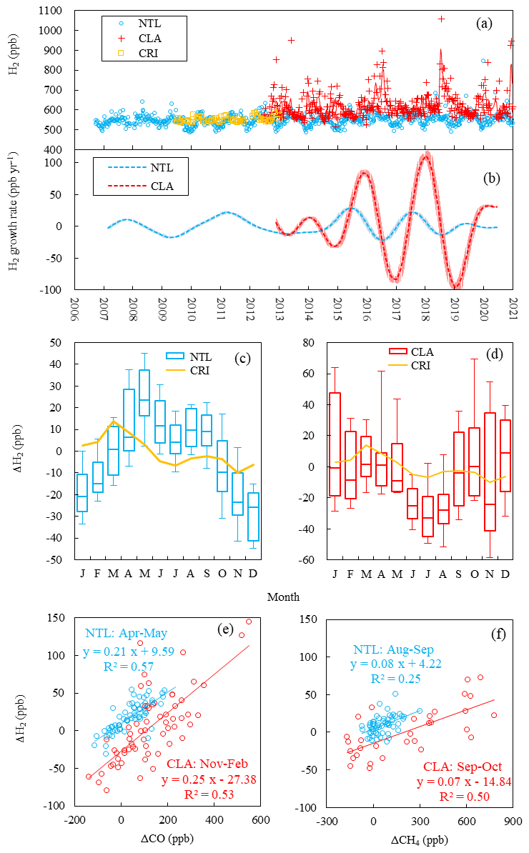
Figure 11 Time series of (a) measured values and (b) growth rate of the atmospheric H₂ mole fraction at NTL, CLA, and CRI in 2006–2020 and seasonal variation in the H₂ mole fraction at (c) NTL and (d) CLA and scatter plots for the relationship of (e) ΔH₂ and ΔCO at NTL during April–May and at CLA during November–February when biomass burning occurred frequently, and (f) ΔH₂ and ΔCH₄ at NTL during August–September and at CLA during September–October when the maximum CH₄ mole fraction was measured.

On the other hand, H₂ is removed from the troposphere by reacting with OH and by deposition and oxidation at surface soil. The amounts of sources and sinks for H₂ in the global budget were estimated to be equal, resulting in a near-equilibrium state (Novelli et al., 1999). The strengths of H₂ removal in the atmosphere over the Indian subcontinent do not differ greatly by region according to Yashiro et al. (2011), whereas the strengths of H₂ sources may differ by region (Price et al., 2007). Lin et al. (2015) reported that H₂ mole fractions at Indian sites were influenced by biomass burning and were 0–40 ppb higher than those at regional background sites (e.g., eastern Kazakhstan and central China). Figure 11c and d show the seasonal variations of the H₂ mole fraction at NTL and CLA, which illustrate the maximum in May and the minimum in December at NTL and the maximum in November–January and the minimum in June–August at CLA, which were different from the averaged seasonal variation in the Northern Hemisphere, which showed the maximum in March–April and the minimum in August–September (Novelli et al., 1999).

Because the burning of biomass (such as harvest residuals and dung) appeared to be actively carried out on the Indo-Gangetic Plain (including at NTL) during April–May and at CLA during November–February, H₂ production must, therefore, increase during these seasons. Furthermore, since higher CH₄ mole fractions at NTL and CLA were observed during August–September and September–October due to strong paddy field emissions at those times, H₂ production from CH₄ degradation can also increase. Figure 11e and f show short-term variable components (such as dCO and dH₂, dCH₄, and dH₂) at both NTL and CLA during those periods and that they had positive correlations. These figures may suggest some relationship between H₂ emission with biomass burning and between photochemical reactions between OH and CH₄, respectively. Furthermore, the minimum H₂ in June–August was influenced by a fresh air mass from the Indian Ocean which is only minimally affected by anthropogenic emission.

As mentioned above, the H₂ mole fraction level at CLA was higher than that at NTL. The amplitude of the seasonal variation of the H₂ mole fraction (Table 2) at CLA showed 70.4 ± 42.2 ppb, which was also larger than the amplitudes at other Indian sites such as Nainital (50 ppb), CRI (50 ppb) (Bhattacharya et al., 2009), HLE (22 ppb), PON (16 ppb), and PBL (22 ppb) (Lin et al., 2015). These tendencies were consistent with the results of Price et al. (2007), which indicated a larger H₂ emission area around the eastern Indo-Gangetic Plain, such as at CLA, than in the western Indian subcontinent. Thus, our observation and previous studies both indicated that the Indian subcontinent had relatively strong H₂ sources.

3.7 N₂O

Garg et al. (2012) reported that the agricultural sector accounted for approximately 75 % of the total N₂O emission in India in 2005, including around 49 % from nitrogen fertilizer use. In particular, they reported that northern India (the Indo-Gangetic Plain) has the highest N₂O emission in India because nitrogen fertilizer was applied to extensive paddy fields and was denitrified and that N₂O was produced and emitted into the atmosphere. Ganesan et al. (2013) reported that the N₂O mole fraction at Darjeeling (northeastern Indian site) was enhanced due to air mass transportation from the Indo-Gangetic Plain. The annual mean N₂O mole fraction at NTL (Table 1) appeared to be almost the same as at the Darjeeling sites in northern India and was higher than at another two Indian sites (CRI; Bhattacharya et al., 2009; and HLE; Lin et al., 2015) and at MLO (Fig. 12a).

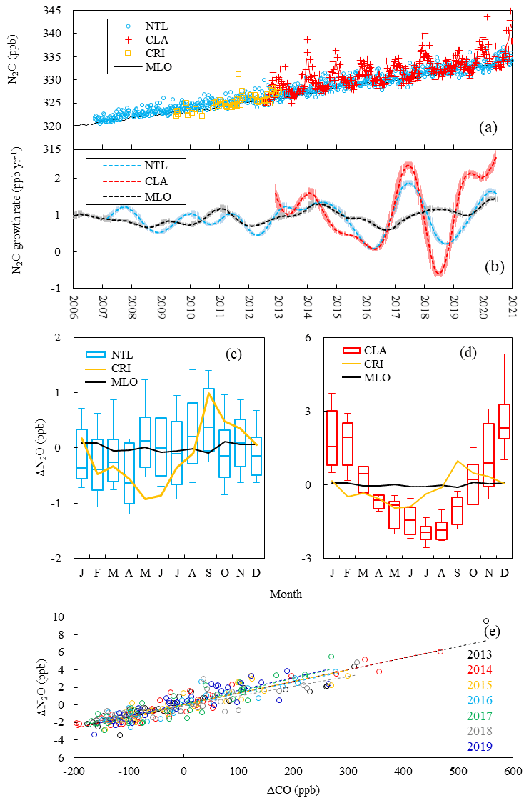
Figure 12 Time series of (a) measured values and (b) growth rates of the N₂O mole fraction at NTL, CLA, and MLO in 2006–2020, seasonal variations in the N₂O mole fraction at (c) NTL and (d) CLA, and (e) the relationship between the ΔN₂O and ΔCO at CLA in 2013–2019.

Thompson et al. (2014) estimated that the N₂O emissions of the eastern Indo-Gangetic Plain, including CLA, were higher than those of the western Indo-Gangetic Plain. This is supported by our observation results that show that the N₂O annual mean mole fraction during 2013–2019 at CLA on the eastern Indo-Gangetic Plain was 1–2 ppb higher than at NTL on the western Indo-Gangetic Plain (Table 1), and the seasonal amplitude of the N₂O mole fraction (Table 2) at CLA (4.25 ± 1.45 ppb) was higher than the amplitudes at other Indian sites (NTL; CRI, Bhattacharya et al., 2009; HLE; PON; and PBL, Lin et al., 2015). Raut et al. (2011) reported the highest N₂O emission rates in the regions of Bangladesh and Sri Lanka due to their high usage of urea as a fertilizer.

However, interestingly, PON and PBL, where oceanic air from the Bay of Bengal affected the sites (Lin et al., 2015), seemed to have relatively higher mole fractions than the sites in this study. As for the seasonal variation in the N₂O mole fraction at NTL, a higher mole fraction was seen in May–September (Fig. 12c). Generally, nitrogen fertilizer was frequently applied to paddy fields in May–September in northern India. Gupta et al. (2016) measured the N₂O flux in paddy fields at New Delhi and reported that the flux increased immediately after the application of nitrogen fertilizer to the fields. Therefore, high N₂O levels and increases in the N₂O mole fraction at NTL in May–September were influenced by the enhancement of the N₂O flux due to the denitrification of nitrogen fertilizer in paddy fields.

The N₂O mole fraction at CLA increased in November–February (Fig. 12d), and such seasonal variation was almost identical to the seasonal variation in CO at CLA. The seasonal component in the N₂O mole fraction (ΔN₂O = deviation of the N₂O mole fraction from the long-term trend) at CLA showed positive correlations (R² = 0.81−0.88) with that of the CO mole fraction (ΔCO) each year (Fig. 11e). Also, their ratio (ΔN₂O $/$ ΔCO) showed 0.013–0.015 ppb ppb⁻¹, which was the same (0.015 ppb ppb⁻¹) as the ratio of total N₂O and total CO emissions in Bangladesh from the EDGAR v4.3.2 database (EC-JRC/PBL, 2016). Although such seasonal variation is likely to be partly related to the lower mixing height in the winter season, variations in N₂O emission flux must affect the seasonal variations in the mole fraction. In general, the CO mole fraction was influenced by biomass burning in this season. Because many inventory data showed that biomass burning produced both N₂O and CO, N₂O may be affected partly by emission from biomass burning. However, the emission ratios of N₂O to CO are fairly variable, with an approximate range of 0.0004–0.017 (Andreae and Merlet, 2001; Sahai et al., 2007, 2011; EDGAR v4.3.2, EC-JRC/PBL, 2016). It seemed that this ratio changes with the types of plants that are burnt. According to Sahai et al. (2011), because the ratio was approximately 0.004 in the case of rice straw, some portion (e.g., 0.004/0.015, i.e., approximately 27 % at the most) of N₂O in the atmosphere may originate from biomass burning. In addition, since Venkataraman et al. (2010) reported that dung burning is one of major N₂O sources among many kinds of biomass burning in India, its contribution was also possible.

On the other hand, nitrification and denitrification processes of nitrogen fertilizer in rice paddy soil are considered to be major causes of N₂O emissions in this region (EDGAR v4.3.2); however, the emission rate appeared to have seasonal variation. Related to the irrigation system, the N₂O flux was thought to be larger in alternating wet and dry conditions than under continuously flooded conditions (Akiyama et al., 2005; Gaihre et al., 2018; Begum et al., 2019). In the summer monsoon season, many rice paddy fields in Bangladesh must have enough water level because of the ample amount of precipitation. After the summer monsoon (from October), the water level in the paddy field intermittently changed with the situation. Therefore, relatively, a higher N₂O emission rate likely occurred during the winter season, when rice (boro rice) was still grown, enhancing the N₂O mole fraction in the winter season. Further observations of high-frequency variations of both N₂O and CO mole fractions will contribute towards precisely evaluating the N₂O emission sources at this site.

The N₂O growth rates at NTL and CLA were similar to that of MLO (Fig. 12b); however, the variations in the N₂O growth rate at both NTL and CLA were larger than that of MLO during 2016–2020. The variation in the N₂O growth rate showed a similar pattern to the growth rates of CO and H₂ (Figs. 9b and 10b), indicating that the sources of these gases had basically common characteristics.

3.8 SF₆

SF₆ is mainly emitted artificially from factories and urban areas (Olivier et al., 2005). Ganesan et al. (2013) reported that the SF₆ emission at Darjeeling (northeastern Indian site) was considerably weak. Our results also showed that SF₆ mole fractions at NTL and CLA were almost the same as the background SF₆ mole fraction (e.g., MLO in Fig. 13a and other sites such as HLE, PON, and PBL, Lin et al., 2015). In addition, the annual amplitudes of the SF₆ mole fraction at Indian sites (HLE, PON, and PBL) were 0.15, 0.24, and 0.48 ppt, respectively, which were almost within the same range (0.15–0.23 ppt) as at NTL and CLA (Table 2). These results suggested that there was no large SF₆ source on the Indo-Gangetic Plain. Figure 13c and d show that the seasonal variations of the SF₆ mole fraction at NTL and CLA decreased in summer (NTL: July, CLA: June–August), which was the same variation as those detected at PON and PBL (Lin et al., 2015). In the summer season, air masses from the south via the Indian Ocean prevailed in the NTL and CLA regions, as shown in Fig. 2. Generally, the SF₆ mole fraction in the Southern Hemisphere was lower than that in the Northern Hemisphere (Geller et al., 1997). Thus, the seasonal variation in the SF₆ mole fraction was explained by the frequency of air mass transportation from the south.

Figure 13 Time series of (a) measured values and (b) growth rates of the SF₆ mole fraction at NTL, CLA, and MLO and the ratios of the air mass from the south at NTL and CLA in 2006–2020 and seasonal variations in the SF₆ mole fraction at (c) NTL and (d) CLA.

Figure 13b shows the interannual variability of the SF₆ growth rate at NTL, CLA, and MLO and southern air mass contribution at NTL and CLA. The variability in the SF₆ growth rate at NTL was different to the variability at MLO, and in fact we could see an anticorrelation between them. In the case of CLA, an anticorrelation was not so clear because of a relatively shorter data record. The decrease in the growth rate at NTL seemed to have a relationship with the increase in the frequency of southern air mass transportation. This indicated that the growth rate of the SF₆ mole fraction at NTL may be controlled by the regional climatic condition though the transportation process. Because SF₆ had weaker sources in northern India, the variation in its trend could be explained more clearly by the influence of the air mass movements.

As mentioned above, anticorrelation in the growth rates between MLO and this region was also seen in CO₂ and CH₄. Therefore, we must take into consideration the influence of the variation in large-scale atmospheric circulation on the GHG mole fraction and trends in their growth rates in the Indian region.

4 Conclusions

We characterized GHGs and related gases over the northern Indian region using air samples collected weekly at Nainital, India (NTL), and Comilla, Bangladesh (CLA), since 2006 and 2012, respectively. Observation data at both NTL and CLA were compared with the GHG data of other Indian sites and Mauna Loa, Hawaii (MLO), at the Pacific station. From this comprehensive analysis, it was found that the features of seasonal and long-term variations in each gas were influenced by the local sinks and sources during each season and annual climatic conditions on the Indo-Gangetic Plain. They were considerably different to those of the MLO in the Pacific region.

On the Indo-Gangetic Plain, rice, wheat, other cereals, and millet are cultivated in the respective seasons corresponding to the change between wet and dry climatic conditions. Therefore, seasonal variations in the atmospheric CO₂ mole fraction were strongly influenced by the crop CO₂ sink at that time. In general, low CO₂ mole fractions in the winter season in the Northern Hemisphere were not observed; however, we observed relatively lower mole fractions during January–March in this region, especially at CLA. In Bangladesh, rice is grown even in the winter season. The δ¹³C-CO₂ signature showed that C₃ plants (e.g., rice and wheat) affected the CO₂ mole fractions in the winter season, while in the summer season the δ¹³C-CO₂ signature showed that C₄ plants (corn, sugarcane, etc.) contributed some portion.

The seasonal variations in δ¹⁸O-CO₂ showed almost the same variation as that in the δ¹⁸O in local rain. Effects of the amount of precipitation and the origin of moisture appeared to affect δ¹⁸O in local rain and CO₂. As a result, δ¹⁸O in CO₂ was affected by the climatic variation related to the amount of precipitation, which was enhanced during 2015–2017. These facts are also consistent with the explanation that CO₂ exchange by photosynthesis (and respiration) by land biomass strongly affected CO₂ seasonality in the mole fraction.

At both sites, higher CH₄ mole fractions were observed than were recorded at other Indian sites. In particular, higher mole fractions than 4000 ppb were recorded at CLA, where rice paddy fields covered the area. Rice cultivation was one of major emission sources in this region. Because CH₄ production activities increased after rice planting, we observed the highest peak in September–October at both sites and a small peak in spring at CLA. A large amount of precipitation during those seasons is likely to have affected the CH₄ production rate of rice paddy fields through soil anaerobic conditions and, as a result, increased the atmospheric CH₄ mole fraction. Air mass transport also influenced seasonal variation and the variability of its growth rate. Besides emissions from rice paddy fields, we identified the relationship between biomass burning and the CH₄ mole fraction in a season other than September–October, when biomass burning occurred frequently. In addition, enteric fermentation and wastewater handling were large emission sources in this region. The large number of sources appeared to increase the average CH₄ mole fraction in this region.

CO was strongly related to biomass burning activities at both sites. The mole fraction was high in the dry season and after crop harvesting. At CLA in winter, a higher mole fraction was observed together with a high N₂O mole fraction, which may suggest some link to biomass burning as a N₂O source. The CO level gradually decreased throughout the observed period. CO emissions must, therefore, be reduced by various technical progresses, including automobile emission and industrial combustion efficiency improvements.

We observed higher N₂O levels in the crop season (i.e., the rainy season) from May to September at NTL but much higher levels in the winter season at CLA. N₂O is known to be mainly emitted from soil though nitrogen fertilizer applications to rice fields and croplands in this region. However, for CLA, we estimated seasonal variations in the emission rate due to the water level in the rice paddy field, because intermittent irrigation in winter generally produces more N₂O than continuously flooded conditions in the rainy season.

H₂ showed the some relationship with both CO and CH₄ mole fractions. We found that CO had a good correlation with H₂ in the biomass burning season, indicating some H₂ contribution from biomass burning. On the other hand, in the season when the CH₄ mole fraction was high, the H₂ mole fraction was also relatively high compared to CH₄, suggesting that chemical reactions of CH₄ and H₂ may contribute some portion of the H₂ mole fraction.

SF₆ showed consistent mole fractions with other Indian sites. Seasonal variations were strongly related to the southern air mass frequency, because the SF₆ mole fraction in the southern region was relatively low.

We found that the interannual variabilities in CH₄, SF₆, and also partly CO₂ growth rates at NTL were anticorrelated with those at MLO, which is located in the Pacific. Growth rates for many GHGs are known to be influenced by El Niño events for many reasons (e.g., hot climate, dry conditions on a global scale). However, in the Indian region, growth rates of some GHGs seemed to be more affected by the regional climate condition such as the Indian Ocean Dipole, which usually affects air circulation and precipitation in the Indian region. In the case of CLA, although the data duration was insufficiently short, growth rates of CO₂, CH₄, and SF₆ changed differently from those at MLO, which could be partly explained by the climatic variations due to the Indian Ocean Dipole. Because CLA is located relatively close to the ocean, sometimes the variation was thought to be different from that at NTL.

These findings have not been reported previously. In this study, long-term records of GHG data at NTL enabled a long-term analysis. These findings suggested that the mole fractions of GHGs and their emissions on the Indian subcontinent could change with climatic conditions in this region in the near future, in addition to changes in anthropogenic activities relating to GHG emissions and countermeasures for the emissions. Therefore, long-term GHG monitoring should be continued, and the effectiveness of countermeasures for reducing GHG emissions on the Indian subcontinent, including the Indo-Gangetic Plain, should be evaluated.