the Creative Commons Attribution 4.0 License.
the Creative Commons Attribution 4.0 License.
 | 08 Nov 2021
Dipole pattern of summer ozone pollution in the east of China and its connection with climate variability
Xiaoqing Ma
Zhicong Yin
Surface O3 pollution has become one of the most severe air pollution problems in China, which makes it of practical importance to understand O3 variability. A south–north dipole pattern of summer-mean O3 concentration in the east of China (DP-O3), which was centered in North China (NC) and the Pearl River Delta (PRD), has been identified from the simulation of a global 3-D chemical transport model for the period 1980–2019. Large-scale anticyclonic (cyclonic) and cyclonic (anticyclonic) anomalies over NC and the PRD resulted in a sharp contrast of meteorological conditions between the above two regions. The enhanced (restrained) photochemistry in NC and restrained (enhanced) O3 production in the PRD contributed to the DP-O3. Decreased sea ice anomalies near Franz Josef Land and associated warm sea surface in May enhanced the Rossby wave source over northern Europe and West Siberia, which eventually induced an anomalous Eurasia-like pattern to influence the formation of the DP-O3. The thermodynamic signals of the southern Indian Ocean dipole were stored in the subsurface and influenced the spatial pattern of O3 pollution in the east of China mainly through the Hadley circulation. The physical mechanisms behind the modulation of the atmospheric circulations and related DP-O3 by these two climate anomalies at different latitudes were evidently verified by large-scale ensemble simulations of the Earth system model.
- Article
(9787 KB) - Full-text XML
-
Supplement
(1352 KB) - BibTeX
- EndNote


Surface O3 is an important air pollutant. Exposure to high concentrations of O3 is detrimental to both human health and vegetation ecology (Rider and Carlsten, 2019). Since 2013, surface O3 concentration has increased over most parts of China, which is largely attributed to changes in anthropogenic emissions (Xu et al., 2018). However, previous studies have shown that in addition to its trend of change, surface O3 concentration also demonstrated large interannual variations with significant regional differences (Zhou et al., 2013; Chen et al., 2019). Based on analysis of 11 years of observational data over Hong Kong, Zhou et al. (2013) reported that the interannual variation in O3 concentration observed during 2000–2010 could reach up to 30 % of the annual average concentration. The O3 concentration in Beijing also showed evident interannual variation during 2006–2016. For example, the O3 concentration in the summers of 2012–2013 was lower by about 10 ppbv than that in 2011 and 2014 (Chen et al., 2019).
High-O3 events are usually associated with meteorological factors (e.g., intense solar radiation, high air temperature, and low humidity) favorable for O3 formation, which can accelerate photochemical reaction and weaken the dispersions and depositions (Han et al., 2020). For example, Lu et al. (2019) designed sensitivity simulations to confirm that ozone pollution in China in 2017 was more serious than that in 2016, which was attributed to the large enhancement of natural emissions of ozone precursors caused by hot and dry climate conditions in 2017. In the summer of 2013, the Yangtze River Delta experienced a severe heat wave with more stagnant meteorological conditions. The upper-level anticyclonic circulation with sink airflows led to abnormally low atmospheric water vapor content above the Yangtze River Delta and thus less cloud cover than normal, which was conducive to a strong solar radiation environment and significant increases in surface ozone (Pu et al., 2017). On the interannual to decadal timescale, anticyclonic anomalies over North China (NC) were critical for O3 distribution in the summer and remotely linked with the effects of Eurasia teleconnection (EU) and west Pacific patterns (Yin et al., 2019).
The Arctic sea ice (SI) declined rapidly while its variability has been increasing over the past decades, which significantly affected summer atmospheric circulations over Eurasia (Lin and Li, 2018). The preceding Arctic SI anomalies could aggravate anomalously high air temperature and drought disasters in NC by triggering EU-like atmospheric responses in summer (Wang and He, 2015). Spring SI anomalies in the Barents Sea could prompt the Silk Road pattern and resulted in a north–south dipole pattern of summer air temperature anomalies in the east of China (Li et al., 2021). When greater-than-normal SI occurred in the Barents Sea, local 500 hPa geopotential height would decrease and a wave chain would form, which subsequently induced more precipitation in the south of East China but less precipitation in the north (Wang and Guo, 2004). Sea surface temperature (SST) in the Pacific and Indian oceans also has significant effects on atmospheric circulation over the east of China (Li and Xiao, 2021; Xia et al., 2021). SST anomalies in the South China Sea and the equatorial eastern Indian Ocean could trigger the East Asian – Pacific pattern and resulted in a dipole pattern of summer temperature and precipitation in the east of China; i.e., areas to the north of the Yangtze River became cold and wet, while areas to the south were hot and dry (Han and Zhang, 2009; Li et al., 2018). Tian and Fan (2019) found that winter SST in the southern Indian Ocean might affect spring–summer SST anomalies near Australia. In summer, the anomalous Hadley circulation in the western North Pacific played an important role in summer precipitation over the middle and lower reaches of the Yangtze River.
Although great attention in previous studies has been paid to the increase in ozone pollution, little is known about changes in the spatial pattern of summer-mean O3 in the east of China. As revealed by Yin and Ma (2020), the dominant pattern of daily-varying ozone pollution in the east of China showed an interannual variation that was mainly driven by the large-scale western Pacific subtropical high and the East Asian deep trough. For example, the frequent movements of the western Pacific subtropical high and the East Asian deep trough both contributed to the out-of-phase variations in O3 over North China and the Yangtze River Delta (Zhao and Wang, 2017; Yin and Ma, 2020). However, to the best of our knowledge, whether the north–south dipole pattern of the summer-mean O3 pollution existed in the east of China still remains unclear. In this study, we attempted to explore the dominant pattern of summertime O3 in the east of China and associated physical mechanisms. Its connections with preceding climate variability were also examined. The remainder of this paper is organized as follows. The data and methods are described in Sect. 2. Section 3 examines the dipole pattern of summertime O3 in the east of China and its possible influencing factors. The associated physical mechanisms are studied in Sect. 4. Major conclusions and discussion are provided in Sect. 5.
2.1 Observations and reanalysis dataset
Hourly ozone concentration observations from 2015 to 2019 are publicly available at https://quotsoft.net/air/ (last access: 23 September 2020). The relevant data were detrended before all computations were conducted for the study period.
The meteorological field data with a horizontal resolution of 0.5∘ latitude by 0.625∘ longitude for the period 1980–2019 were taken from the MERRA-2 dataset (Gelaro et al., 2017), including geopotential height at 500 hPa (Z500), surface incoming shortwave flux (Ssr), low and medium cloud cover (Mlcc), precipitation (Prec), 10 m zonal and meridional winds (UV10 m), and surface air temperature (SAT) and zonal and meridional winds and vertical velocity at different vertical levels. Monthly outgoing longwave radiation (OLR) data () could be acquired from the University of Maryland OLR Climate Data Record portal (http://olr.umd.edu/, last access: 28 May 2021). Monthly SI concentrations and SST () for the period 1980–2019 were downloaded from the website of the Met Office Hadley Centre (Rayner et al., 2003). Monthly mean subsurface ocean temperatures in the upper 250 m with a horizontal resolution of were obtained from the Met Office Hadley Centre EN4 version 2.1 (Good et al., 2013).
The wave activity flux (WAF) was computed to illustrate the propagation of Rossby wave activities (Takaya and Nakamura, 2001):
where subscripts denote partial derivatives; the overbar and prime represent the climatological mean and anomaly, respectively; and ψ′ represents the stream function anomaly. U is the horizontal wind speed; u and v are the zonal and meridional wind components, respectively; and W denotes the two-dimensional Rossby WAF. The Rossby wave source proposed by Sardeshmukh and Hoskins (1988) is also calculated in this study. V, ξ, and f refer to the horizontal wind velocity, relative vorticity, and geostrophic parameter, respectively. ∇ is the horizontal gradient; the subscript χ represents the divergent component.
2.2 1980–2019 O3 concentrations simulated by GEOS-Chem
Hourly ozone concentrations were simulated by the nested-grid version of the global 3-D chemical transport model (GEOS-Chem), which included a detailed description of oxidant–aerosol chemistry. The model was driven by MERRA-2 assimilated meteorological data (Gelaro et al., 2017). The nested grid over China (15–55∘ N, 75–135∘ E) had a horizontal resolution of 0.5∘ latitude by 0.625∘ longitude and consisted of 47 vertical layers up to 0.01 hPa. The GEOS-Chem model included the fully coupled O3–NOx–hydrocarbon and aerosol chemistry modules with more than 80 species and 300 reactions (Bey et al., 2001).
Chemical and physical processes were examined using the outputs of GEOS-Chem. Because non-local planetary boundary layer (PBL) mixing was used, emissions and dry deposition trends within the PBL were applied within the mixing (Holtslag and Boville, 1993). Compared with other terms, the value of wet deposition was extremely small, so it was not considered in this study (Liao et al., 2006). Consequently, the major chemical and physical processes related to meteorological conditions included chemistry, convection, PBL mixing, transport, and their sum within the PBL.
The GEOS-Chem model has been widely used to examine historical O3 changes in China. Yang et al. (2014) evaluated the simulated interannual variation in June–July–August (JJA) surface-layer O3 concentration at the Hok Tsui station (22∘13′ N, 114∘15′ E). They found that the model could capture the peaks and troughs of the observed JJA O3 concentration well with a high correlation coefficient of +0.87 (exceed the 99 % confidence level) between simulations and observations. Moreover, the model could also realistically simulate the spatial distribution of O3, and the spatial correlation coefficient between simulations and observations in the summer of 2017 could reach up to 0.89 (Li et al., 2019). These studies indicated that the GEOS-Chem model could capture the interannual variation and distribution of the surface O3 concentration fairly well.
The GEOS-Chem model successfully reproduced the dominant patterns of summer O3 pollution on a daily scale from 2015 to 2019 (Yin and Ma, 2020). In this study, we first simulated the maximum daily average 8 h concentration of O3 (MDA8 O3) from 2015 to 2019 and evaluated the performance of GEOS-Chem. The simulated spatial distribution of MDA8 O3 was similar to that of observations, with a spatial correlation coefficient of 0.87 (Fig. 1a). We compared the simulated and observed summer-mean MDA8 O3 concentrations in NC and the Pear River Delta (PRD), which had a low bias with a mean absolute error of 5.7 and 12.1 µg m−3 in the PRD and NC, respectively. The values of root-mean-square error/mean were 15.8 % and 8.1 % in NC and the PRD, respectively. The observed and simulated summer MDA8 O3 anomalies in the east of China also presented consistent interannual differences (Fig. S1a and b in the Supplement). The high consistency in both the temporal and spatial distributions between the simulations and observations provided solid evidence to support the feasibility of the present study.
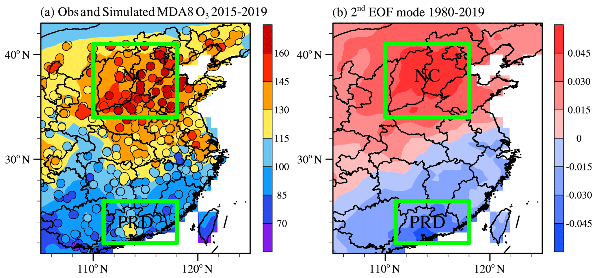
Figure 1(a) Spatial distributions of observed (dots) and GEOS-Chem-simulate (shading) summer-mean MDA8 O3 (unit: µg m−3) for the period 2015–2019. (b) The second EOF spatial pattern of simulated summer-mean MDA8 O3 from 1980 to 2019. The simulated O3 concentrations were produced by GEOS-Chem with fixed emissions but changing meteorological conditions from 1980 to 2019. The green boxes represent the areas of NC and the PRD.
Based on the above results, the GEOS-Chem model was then driven by fixed anthropogenic and natural emissions in 2010 and changing meteorological fields from 1980 to 2019 to highlight the impact of climate variability on O3 concentration. Results of this simulation were analyzed to reveal the dominant pattern of ozone pollution in the east of China in summer and its relationship with preceding climate anomalies.
2.3 Numerical experiments with CESM-LE
To provide evidence that supports the proposed connections between SI and SST and large-scale atmospheric circulations, the simulations of the Community Earth System Model Large Ensemble (CESM-LE) were employed (Kay et al., 2015). The CESM consists of coupled atmosphere, ocean, land, and sea ice component models. The 40-member ensemble of CESM-LE simulations over the period 1980–2019 includes a historical simulation (1980–2005) and a Representative Concentration Pathway (RCP) 8.5 forcing simulation (2006–2019). To confirm the impact of preceding climate variability and associated physical mechanisms, composite analyses were conducted based on the 3 years with the lowest and highest simulated preceding climatic variability for a particular month in each member. The composite results of atmospheric circulations could be considered as the relevant atmospheric responses associated with the preceding climate variability.
As aforementioned, the GEOS-Chem model has a good performance in simulating O3 concentration. The summer O3 concentrations from 1980 to 2019 were simulated by GEOS-Chem, and the EOF approach was applied to the GEOS-Chem simulation to explore the dominant patterns of summer-mean O3 pollution in the east of China. Percentage contributions to the total variance by the first and second EOF modes were 39 % and 17.5 %, respectively. The significance test of the EOF eigenvalues confirmed that the first and second patterns were distinctly separated (passing the North test; North et al., 1982). The first EOF pattern displayed a monopole pattern (Fig. S2). The second EOF pattern presented a north–south dipole pattern of O3 (DP-O3) distribution in the east of China with the two centers located in NC and the PRD (Fig. 1b). Observations have shown that high O3 concentration frequently occurs in NC, and O3 pollution in the PRD has become increasingly serious in recent years (Liu et al., 2020). Furthermore, about 80 % of the MDA8 O3 anomalies in NC were in opposite sign to those in the PRD during 2015–2019 (Fig. S1a and b). Therefore, despite the fact that it was only the second leading EOF mode, we still focused on the investigation of DP-O3 in the present study, since it was more similar to the actual pollution situation. Impacts of climate variability are also analyzed.
The MDA8 O3 anomalies were divided into positive (P) and negative phases (N) of DP-O3 (Fig. S3). For convenience, DP-O3P and DP-O3N were defined by the EOF time series of DP-O3 greater than 1 SD (standard deviation) and less than , respectively. The DP-O3P corresponded to positive anomalies of MDA8 O3 in the north and negative anomalies in the PRD (Fig. S3a). In contrast, high concentration of O3 occurred in the PRD, and a low-concentration center appeared in NC under the DP-O3N condition (Fig. S3b). The correlation coefficient between time series of DP-O3 and MDA8 O3 difference between NC and the PRD was 0.91, indicating that DP-O3 reflected the opposite changes of O3 concentration in NC and the PRD.
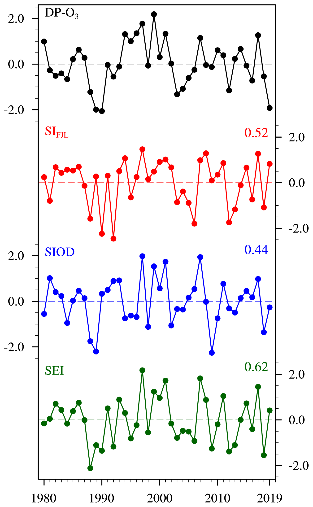
Figure 2Variations in standardized DP-O3 time series (black), May SI near Franz Josef Land (SIFJL, red), January–February–March mean Subtropical Indian Ocean Dipole (SIOD, blue), and SEI (green) from 1980 to 2019. SEI is defined as the weighted average of SIFJL and SIOD. The correlation coefficients of the DP-O3 with SIFJL (red), SIOD (blue), and SEI (green) were shown in the figure.

Figure 3Composite summer atmospheric circulations associated with the DP-O3 (DP-O3P minus DP-O3N) for the period 1980 to 2019, including (a) surface air temperature (SAT, unit: K, shadings) and geopotential height at 500 hPa (unit: 10 gpm, contours), (b) surface incoming shortwave flux (Ssr, unit: W m−2, shadings) and low and medium cloud cover (Mlcc, unit: 1, contours), and (c) precipitation (Prec, unit: mm, shadings) and surface wind (unit: m s−1, arrows). The white dots indicate that the composites with shading were above the 90 % confidence level. The black boxes in (a) indicate the centers of the ACNC and CPRD, respectively. The green boxes in (b) and (c) represent the areas of NC and the PRD. Composites of the summer mass fluxes of O3 (d) associated with the DP-O3 (DP-O3P minus DP-O3N) for the area-averaged differences (NC minus PRD) from 1980 to 2019. The bottom axis gives the names of the chemical and physical processes: chemical reaction (Chem), convection (Conv), PBL mixing (Mix), transport (Trans), and their sum (Sum).
With fixed emissions, the changes in O3 concentrations from 1980 to 2019 were solely caused by meteorological conditions. The time series of DP-O3 showed a strong interannual variation (Fig. 2). Composite differences in large-scale atmospheric circulation and meteorological conditions related to DP-O3 between the positive and negative phases (DP-O3P minus DP-O3N) were analyzed to explore the impacts of atmospheric circulation on photochemical reactions and accumulations of various pollutants in the above two areas. During the positive phase of DP-O3, cyclonic and anticyclonic anomalies in the middle troposphere were found over the PRD and NC (CPRD and ACNC) (Fig. 3a), respectively. The CPRD and accompanied southerly winds in the PRD efficiently transported clean and moist air from the sea to the PRD (Fig. 3c). Furthermore, low and medium cloud covers were significantly increased, which led to weak solar radiation and reduced photochemical reactions (Fig. 3b). A moist, cool environment and weak solar radiation were conducive to low O3 concentration in the PRD. On the other hand, the positive anomalies of geopotential height in NC increased surface air temperature (Fig. 3a), resulting in a dry environment with decreased cloud cover and sunny weather (Fig. 3b and c).
In order to provide a more quantitative evaluation of the contribution of chemical and physical processes, in Fig. 3d, we examine the area-averaged differences in O3 changes for NC and the PRD. Chemistry represents the changes in net chemical production, which appears to be the dominating process, leading to the greatest O3 change between NC and the PRD (12.3 t d−1, Fig. 3d). Transport represents the change in horizontal and vertical advection of ozone. Depending on the ozone concentration gradient and wind anomalies, the transport difference between NC and the PRD is 3.1 t d−1 (Fig. 3d). Convection changes slightly in NC and the PRD. As the mixing process transports ozone along the vertical concentration gradient, it generally contributes negatively to the total ozone change. The above analysis indicates that different meteorological conditions between NC and the PRD led to the difference of O3 concentration in the two regions (differed by 5.2 t d−1), which eventually contributed the formation of DP-O3.
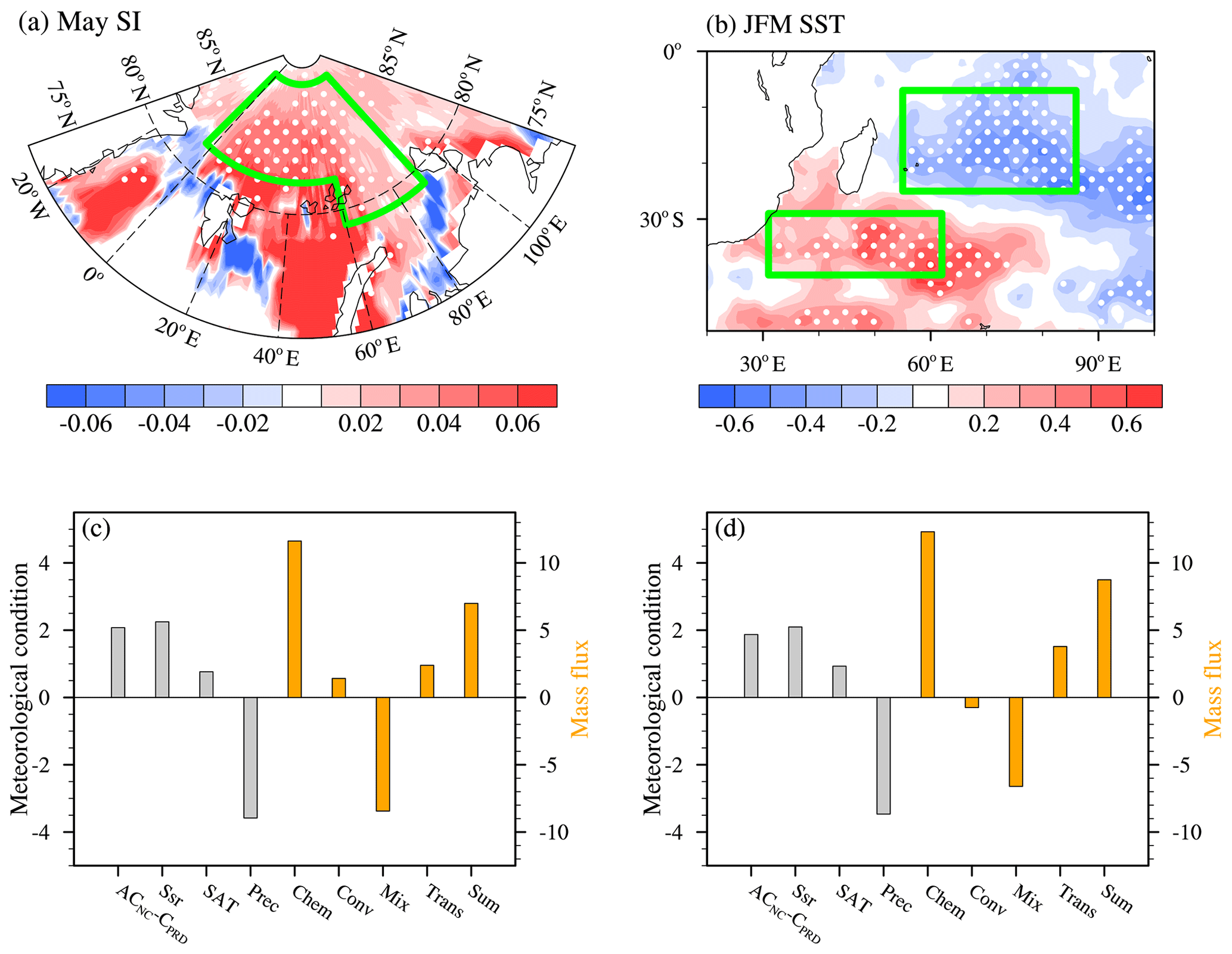
Figure 4Composites of (a) May SI concentration and (b) JFM SST associated with the DP-O3 (DP-O3P minus DP-O3N) from 1980 to 2019. The green boxes in (a) and (b) indicate where the SIFJL and SIOD indices are calculated, respectively. The white dots indicate that the composites were above the 90 % confidence level. Composite summer meteorological conditions, circulations, and mass fluxes of O3 associated with (c) SIFJL (positive SIFJL years minus negative SIFJL years) and (d) SIOD (positive SIOD years minus negative SIOD years) from 1980 to 2019. The bottom axis gives the names of the meteorological conditions and chemical and physical processes: the differences between ACNC and CPRD (unit: 10 gpm), surface incoming shortwave flux (Ssr, unit: W m−2), surface air temperature (SAT, unit: K), precipitation (Prec, unit: mm), chemical reaction (Chem, unit: t d−1), convection (Conv, unit: t d−1), PBL mixing (Mix, unit: t d−1), transport (Trans, unit: t d−1), and their sum (Sum, unit: t d−1).
Arctic SI in May was closely related to summer O3 pollution in NC (Yin et al., 2019), but its effects on the north–south dipole distribution of O3 had not been studied. The meridional O3 dipole pattern in the east of China was positively correlated with SI anomalies near Franz Josef Land (SIFJL). Note that the correlation between them remains unchanged after the signal of El Niño–Southern Oscillation (ENSO) was removed. The area-averaged (82–88∘ N, 3∘ W–60∘ E; 79–88∘ N, 60–90∘ E; denoted by the green boxes in Fig. 4a) SI in May was calculated and defined as the SIFJL index, whose linear correlation coefficient with the time series of DP-O3 was 0.52 (exceeding the 99 % confidence level). When the SIFJL anomalies were significant (i.e., |anomalies| > its one standard deviation), the occurrence probability of the DP-O3 in the same phase was 83 % (Fig. 2). Furthermore, the active centers of the anomalous atmospheric circulations and meteorological conditions associated with SIFJL in the east of China were similar to those of the DP-O3 (i.e., NC and the PRD). That is, positive SIFJL anomalies were conducive to less (more) precipitation, less (more) cloud cover, and strong (weak) solar radiation in NC (PRD) (Figs. 4c and S4). The chemical and physical processes of ozone production in GEOS-Chem simulations were analyzed. The difference of chemical reactions between NC and the PRD had a large positive value (11.6 t d−1), and the difference of the sum of all chemical and physical processes was 7.0 t d−1 (Fig. 4c), resulting in DP-O3.
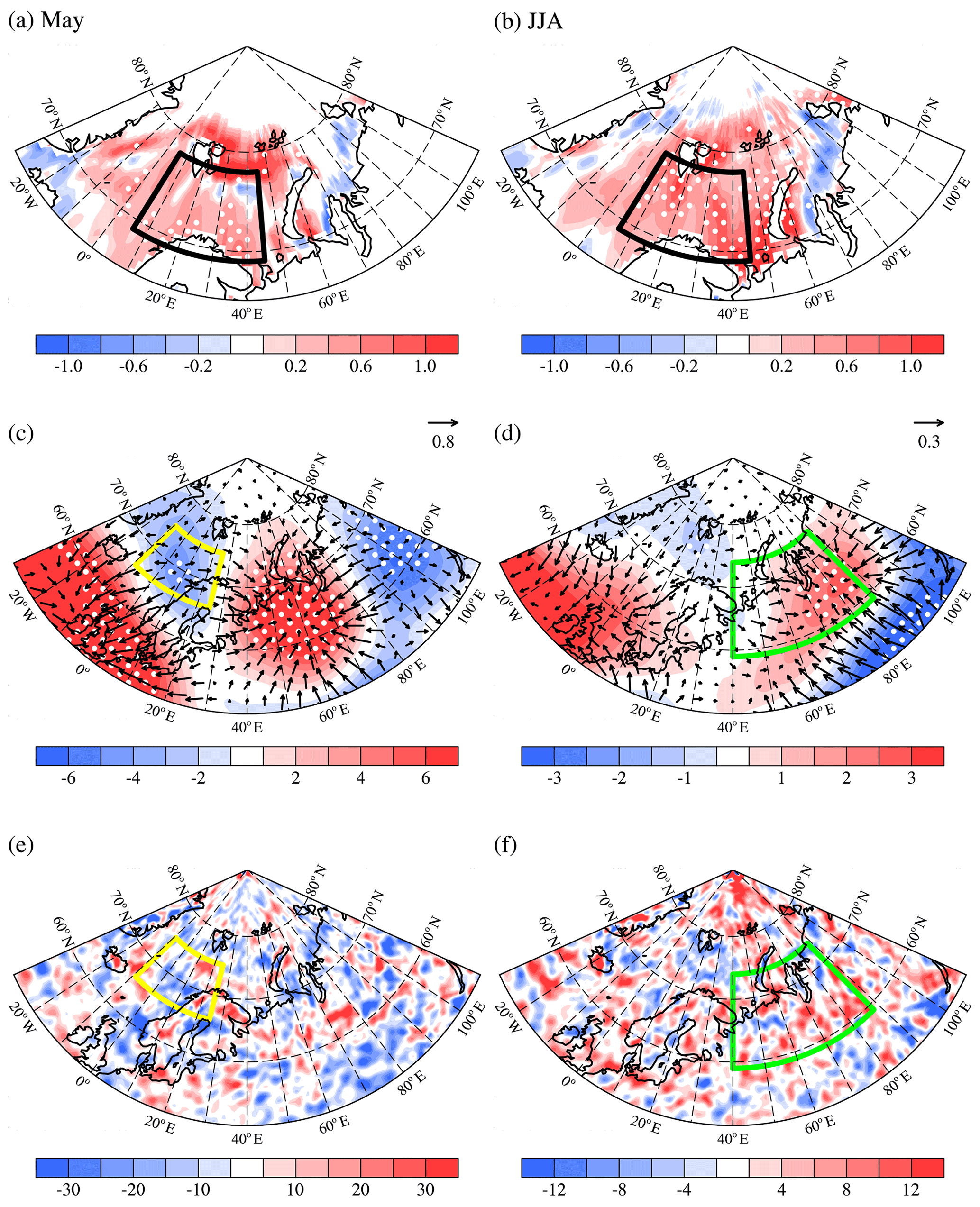
Figure 5Composites of (a) May Arctic SST (unit: K), (c) velocity potential (unit: 105 m2 s−1, shading) and divergent wind at 500 hPa (unit: m s−1, arrows), and (e) Rossby wave source anomalies at 500 hPa (unit: 10−11 s−2) associated with SIFJL index (negative SIFJL years minus positive SIFJL years) from 1980 to 2019. The black box in (a) and (b), yellow box in (c) and (e), and green box in (d) and (f) represent the center of the SST, velocity potential, and Rossby wave source anomaly associated with SIFJL, respectively. The white dots indicate that the composites with shading were above the 90 % confidence level.
In addition to the signal from the Arctic, SST as an effective external forcing also has significant influences on summer climate in the east of China (Li et al., 2018). Therefore, it was important to answer the question whether SST could affect the DP-O3 in the east of China in summer. Large anomalies of preceding January–February–March (JFM) SST over the southern Indian Ocean were obvious when we evaluated the relationship between the DP-O3 and previous SST. After removing the influence of ENSO, the SST signal in the southern Indian Ocean still remains (Fig. 4b). The two regions with significant anomalies were similar to the Subtropical Indian Ocean Dipole (SIOD) regions found by Behera and Yamagata (2001). Variance analysis and correlation analysis of SST in the Indian Ocean also indicated that a SST dipole type oscillation occurred in the southern Indian Ocean, which usually developed in the preceding winter and reaches its strongest in the subsequent January to March (Jia and Li, 2013). The difference between the mean SST of the two regions (29–40∘ S, 31–62∘ E and 7–25∘ S, 55–86∘ E; green box in Fig. 4b; the southwest positive pole minus the northeast negative pole) was defined as the SIOD index and calculated (Fig. 2). The linear correlation coefficient between the SIOD index and the time series of DP-O3 from 1980 to 2019 was 0.44 (significant at the 99 % confidence level). When the SIOD anomalies were significant (i.e., |anomalies| > its 1 standard deviation), the occurrence probability of DP-O3 in the same phase is 82 % (Fig. 2). Furthermore, the composite meteorological conditions in the positive and negative phases of SIOD had similar centers to that of DP-O3. That is, the anticyclone over NC was always accompanied by hot–dry meteorological conditions, while the cyclone over the PRD was always accompanied by a cool–moist environment (Figs. 4d and S5). The chemical reactions increased 12.3 t d−1 in NC compared to those in the PRD (Fig. 4d), indicating that the strong solar radiation and high-temperature conditions actually enhanced the chemical reactions in the atmosphere to produce more O3 in NC.

Figure 6Composites of (a) wave activity flux anomalies (unit: m2 s−2, arrows), geopotential height (unit: gpm, shading) at 500 hPa, and (b) mean wind (unit: m s−1, arrows), omega (unit: 10−2 Pa s−1, shading) over 100–130∘ E, and the anomalies of ACNC and CPRD (unit: gpm, bar) in summer associated with SIFJL index (negative SIFJL years minus positive SIFJL years) from 1980 to 2019. The green boxes in (a) represent the centers of the EU-like pattern. The white dots indicate that the composites with shading were above the 90 % confidence level.
Changes in SIFJL and SIOD could both possibly contribute to the formation of DP-O3. Note that SIFJL and SIOD have few years of common significant anomalies; more than 78 % of the individual sample years were used to make a composite with both indices. The correlation coefficient between them was only 0.21 and was not significant, indicating that SIFJL and SIOD were independent of each other. Several previous studies have documented that the preceding Arctic SI anomalies could trigger EU-like atmospheric responses in the subsequent summer and thus influenced the climate in the east of China (Wang and He, 2015). Corresponding to reduced SIFJL, SST anomalies in the Barents and Kara seas were significantly positive and gradually increase from May to summer months (Fig. 5a and b). The warm SST anomalies influenced local heat anomalies and caused anomalous atmospheric circulations. Following the decrease in SIFJL, anomalous divergent winds appeared in the mid-troposphere, which were accompanied by warm SST anomalies and negative velocity potential anomalies (yellow box in Fig. 5c). As proposed by Xu et al. (2021), the rotational component of the anomalous divergent winds could spread to the south and force the vorticity generation over Eurasia. Thus, during the subsequent summer, significant convergence and positive velocity potential with a positive Rossby wave source anomaly occurred over northern Europe and West Siberia (green box in Fig. 5d). We also used the SST anomalies associated with SIFJL (in Barents and Kara seas in JJA) to composite relevant variables. Significant convergence, positive velocity potential, and positive Rossby source anomaly all appeared over Europe and West Siberia in JJA (Fig. S6). This indicated that positive anomalies of Rossby wave source over Europe and West Siberia could be generated by local heat anomalies associated with decreased SIFJL in the Barents and Kara seas.
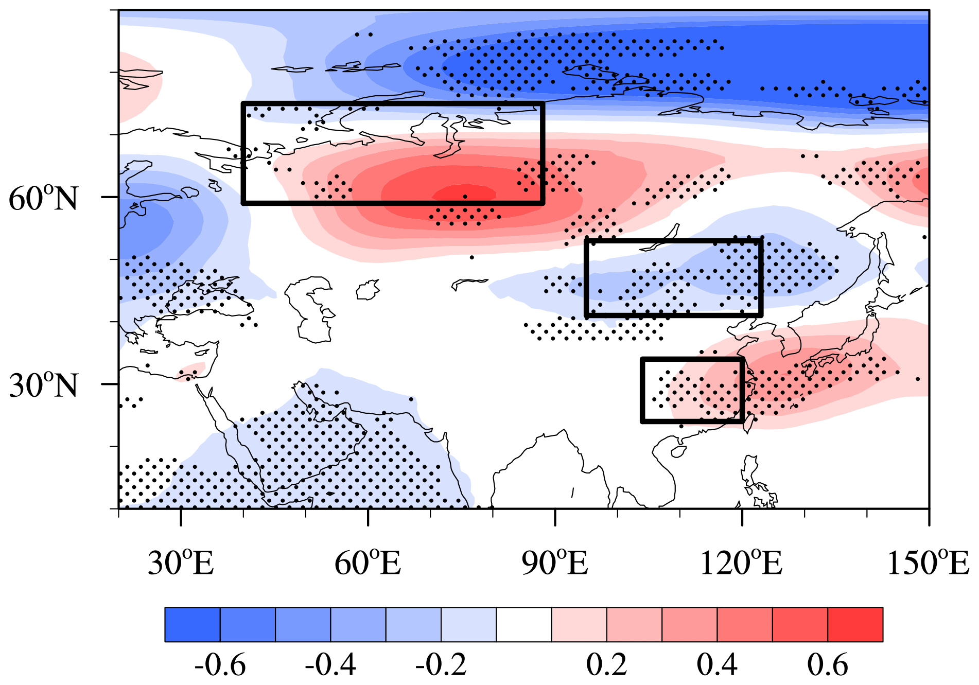
Figure 7Composite differences of geopotential height at 500 hPa in JJA between three low- and high-SIFJL years based on the ensemble of 40 CESM-LE simulations during 1980–2019. The black dots indicate that the mathematical sign of the composite results of more than 60 % of the members is consistent with the ensemble mean. The black boxes represent the centers of the EU-like pattern.
Moreover, corresponding to the decreased SIFJL, the anomalous Rossby WAF propagated from Europe and West Siberia (consistent with the aforementioned Rossby wave source) to northeast China and enhanced the cyclonic anomaly nearby (Fig. 6a). The anomalous cyclonic circulation caused ascending motion from the surface up to 300 hPa over NC and further induced a meridional circulation with an anomalous descending branch near 20∘ N (Fig. 6b). Likewise, an anomalous anticyclone occurred in the middle troposphere above the PRD (Fig. 6b). In other words, an EU-like Rossby wave train was induced in the mid-troposphere (Fig. 6a), which propagated from northern Europe and the West Siberian Plain (+), reaching the broad area from northeastern China (−) to the south of China (+). Thus, the reduction in SI near Franz Josef Land in May modulated the EU-like pattern in the subsequent summer and strengthened the anomalous cyclonic and anticyclonic circulations over NC and the PRD (Fig. 6b), respectively. The differences in anomalous atmospheric circulations and associated meteorological conditions between NC and the PRD make great contributions to the occurrence of DP-O3.
The relationship between the preceding May SI anomalies and the JJA EU-like pattern was also confirmed by large ensemble simulations of CESM during 1980–2019. According to the simulated sea ice fraction near Franz Josef Land, the 3 years with the lowest and highest SI in each member were selected to construct the composite maps based on all 40 available members. The difference in JJA geopotential height at 500 hPa represented the atmospheric response to declining May SIFJL. As shown in Fig. 7, the decline of SIFJL in May led to an EU-like pattern in the subsequent summer over Eurasia, which was in good accordance with the observed result (Fig. 6a). The anticyclonic and cyclonic anomalies shown in the geopotential height at 500 hPa (i.e., ACNC and CPRD) in summer were also well reproduced by over 60 % of the members. The above results confirmed the robustness of the physical mechanisms proposed in the present study.
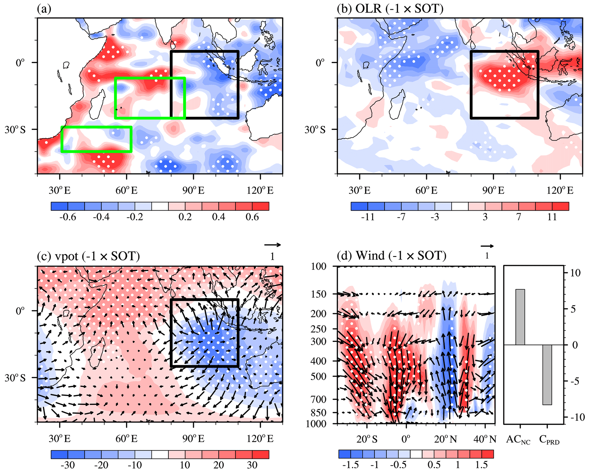
Figure 8(a) Composites of mean 0–60 m subsurface ocean temperature (unit: K) in summer associated with the SIOD (positive SIOD years minus negative SIOD years) from 1980 to 2019. The green boxes represent the centers of the SIOD, and the black box indicates where the SOT index is calculated. Composites of (b) OLR (unit: W m−2) and (c) velocity potential (unit: 105 m2 s−1, shadings) and divergent winds (unit: m s−1, vectors) at 10 m in summer associated with SOT indexes of opposite sign (negative SOT years minus positive SOT years). The black box represents the center of the SOT. (d) Composites of summer-mean winds (unit: m s−1, arrows) and omega (unit: 10−2 Pa s−1, shadings) over 90–120∘ E, and the anomalies of ACNC and CPRD (unit: gpm, bars) associated with SOT indexes of opposite sign. The white dots indicate that the composites with shading were above the 90 % confidence level.
SIOD could influence atmospheric anomalies and distribution of summer precipitation in China mainly through Hadley circulation (Liu et al., 2019). Can SIOD anomalies also influence the DP-O3 via meridional atmospheric forcing? Despite the significant correlation between SIOD anomalies (defined by SST) and the DP-O3 in the east of China (Fig. 4b), it should be noted that the thermodynamic signals in the southern Indian Ocean not only existed on the sea surface but also extended to the subsurface (Fig. S7). As time goes by, the center of negative SST anomalies moved to the northeast possibly due to the eastward movement of atmospheric forcing caused by the mean westerly flow (Behera and Yamagata, 2001). When it moved to the vicinity of Sumatra Island in JJA, the abnormally cold signals of SST could extend downward from the surface to 60 m (black box in Fig. 8a). The area-averaged (black box in Fig. 8a) summer-mean subsurface ocean temperature of 0–60 m was defined as the SOT index and calculated. Affected by negative SOT anomalies near Sumatra Island, the equatorial eastern Indian Ocean convection was suppressed (indicated by positive anomalies of OLR in Fig. 8b), and significant divergence prevailed in the lower troposphere (Fig. 8c). As a result, anomalous downward air flow developed near Sumatra Island from 300 hPa to the surface (about 20–5∘ S in Fig. 8d). This anomalous downward air flow modulated the meridional circulation over 90–120∘ E by strengthening the abnormal upward airflow at 20∘ N and downward airflow at 30∘ N. Thus, the ACNC and CPRD were enhanced simultaneously (Fig. 8d). Overall, following the positive phase of SIOD, the cold signal of SOT anomalies changed the meridional circulation in the subsequent JJA and strengthened the CPRD and ACNC in the troposphere above the east of China. Under these large-scale atmospheric anomalies, O3 concentrations became higher in NC, whereas the generation of surface O3 was weakened in the PRD.
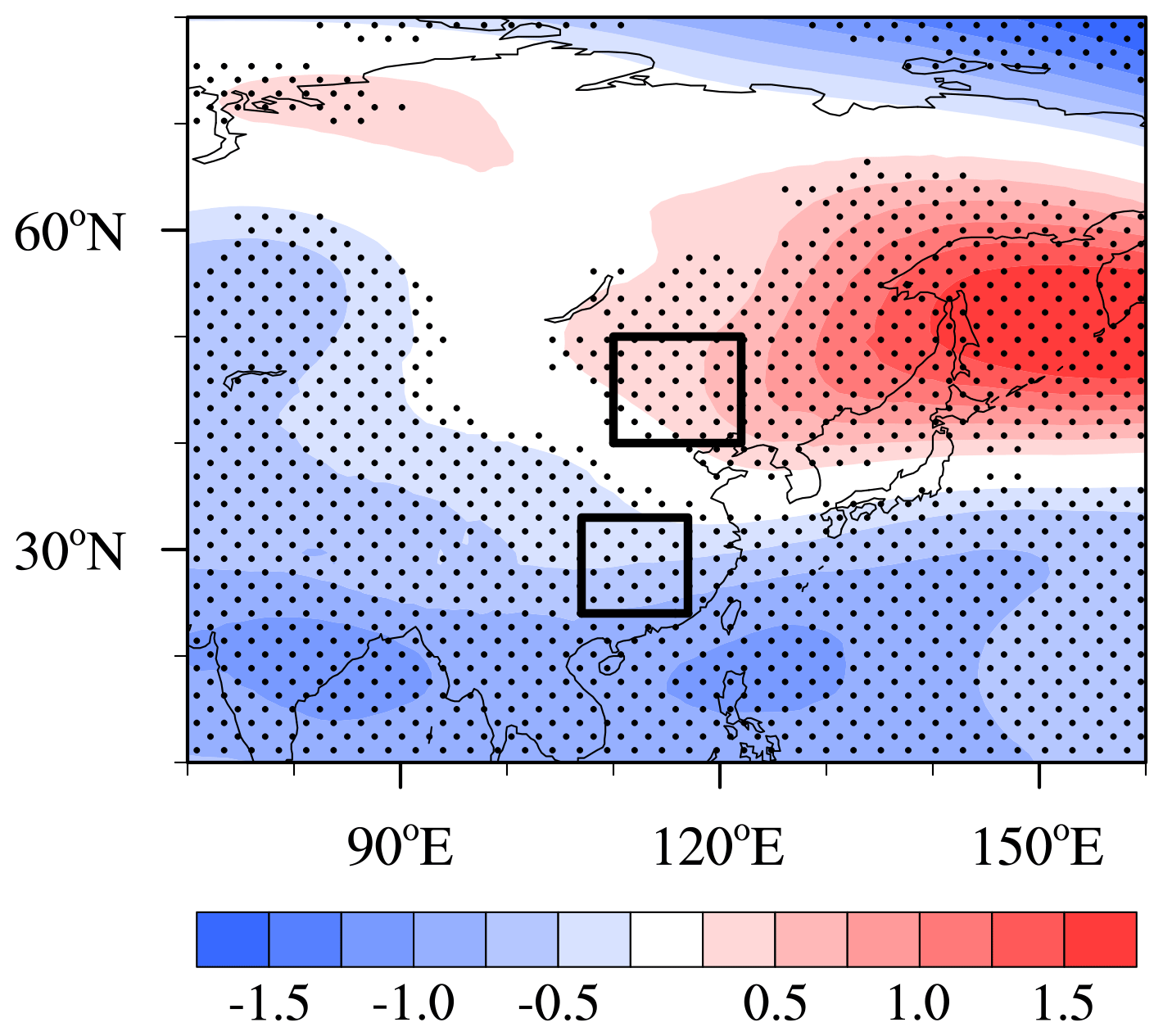
Figure 9Composite differences of geopotential height at 500 hPa in JJA between three high- and low-SIOD years based on the ensemble of 40 CESM-LE simulations during 1980–2019. The black dots indicate that the mathematical sign of the composite results of more than 60 % of the members is consistent with the ensemble mean. The black boxes represent the centers of ACNC and CPRD, respectively.
The CESM-LE datasets were also used to verify the statistical correlation between the preceding SIOD and large-scale atmospheric circulations in JJA. The composite differences of SIOD in JFM between the 3 high years and 3 low years of SST simulated by each ensemble member during 1980–2019 were investigated based on the ensemble of 40 CESM-LE simulations. The composite results (positive SIOD years minus negative SIOD years) of atmospheric circulations could be considered the relevant atmospheric circulation responses associated with differences in SIOD. More than 60 % of the CESM ensemble members could reproduce the anticyclonic circulation over NC and the cyclonic circulation over the PRD in summer at 500 hPa well (Fig. 9). That is, the CESM-LE also confirmed the relationship between the previous JFM SIOD anomaly and the DP-O3-related atmospheric circulations (i.e., ACNC and CPRD) in subsequent JJA.
In general, the O3 concentrations in NC were substantially high, and the problem of O3 pollution in the PRD has become increasingly prominent in recent years. A south–north dipole pattern of O3 concentration in the east of China was identified based on GEOS-Chem simulations with fixed emissions and changing meteorological conditions from 1980 to 2019. The DP-O3 pattern presented opposite centers in NC and the PRD. Corresponding to the positive phase of DP-O3, cyclonic and anticyclonic anomalies were located over the PRD and NC, respectively, which resulted in a dry and hot climate in NC, while the environment in the PRD region was cool and moist. The opposite was true in the negative phase of DP-O3. During positive phases, the meteorological conditions mentioned above significantly enhanced photochemical reactions in NC but suppressed O3 production in the PRD and thus make great contributions to the south–north dipole pattern of O3 in the east of China.
Arctic SI near Franz Josef Land in May played an important role in the occurrence of DP-O3. The warm SST anomalies associated with less SIFJL could induce divergent wind field and vorticity advection in the upper layer and enhanced positive Rossby wave source over northern Europe and West Siberia in summer. An EU-like pattern was triggered in Eurasia (solid lines in Fig. 10), which could enhance the DP-O3-related atmospheric circulation (i.e., ACNC and CPRD) in JJA. As a result, meteorological conditions for O3 concentration were completely different between NC and the PRD, which eventually contributed to the formation of DP-O3. In addition, the precursory climatic driving signal of SIOD anomalies in the low latitudes in JFM was also closely linked to DP-O3. The thermodynamic signal of SIOD could be stored in the subsurface, and the center of negative SST anomalies moved to the vicinity of Sumatra Island in summer. The meridional circulation intensified in summer (dashed lines in Fig. 10), which, along with the enhancement of the ACNC and CPRD over the east of China, effectively increased O3 concentration in NC but suppressed the generation of surface O3 in the PRD. The linkages and corresponding physical mechanisms were well reproduced by the large CESM-LE ensemble simulation.

Figure 10Schematic diagrams of the associated physical mechanisms. The May SI anomalies near Franz Josef Land (red shadings) could trigger an EU-like pattern in the atmosphere in summer, which enhances the anticyclonic anomaly over NC and the cyclonic anomaly over the PRD. The thermodynamic signal of the preceding SIOD (contours) could be stored in the subsurface, and the center of negative SST anomalies moves to the vicinity of Sumatra in summer (blue shading). The meridional circulation was enhanced in summer (dashed lines), along with the enhancement of ACNC and CPRD over eastern China. The solid lines indicate the anomalous atmospheric circulations affected by SIFJL, while the dashed lines indicate the anomalous atmospheric circulations affected by SIOD.
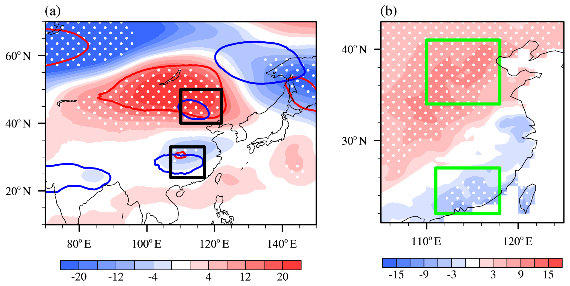
Figure 11(a) Composites of geopotential height at 500 hPa (unit: gpm, shadings) in summer associated with the SEI (positive SEI years minus negative SEI years) from 1980 to 2019. The red and blue lines indicate areas where the composite geopotential height anomalies associated with SIFJL and SIOD exceed the 90 % confidence level, respectively. The black boxes represent the centers of ACNC and CPRD, respectively. (b) Composite differences of the detrended summer-mean MDA8 O3 (unit: µg m−3) simulated by GEOS-Chem model between high- and low-SEI years during 1980–2019. The white dots indicate that the composite differences are above the 90 % confidence level. The green boxes represent the areas of NC and the PRD.
The above analysis has revealed that the DP-O3 is independently affected by SIOD and SIFJL from 1980 to 2019. We attempted to discuss the combined impacts of the two precursory climatic drivers in the present study. For this purpose, a synthetic climate variability index SEI, defined as the weighted average of SIFJL and SIOD, is calculated by
where r1 and r2 were the correlation coefficients of SIFJL (r1=0.52) and SIOD (r2=0.44) with the DP-O3 time series, respectively. The correlation coefficient between SEI and DP-O3 was 0.62 (Fig. 2, exceeding the 99 % confidence level). When the SEI anomalies were significant, the occurrence probability of the DP-O3 in the same phase was 93 % (Fig. 2), which is higher than that based on individual influences of the two factors. Composite atmospheric circulation analysis has been carried out based on years of positive and negative SEI anomalies, and the results are shown in Fig. 11a. The composite atmospheric circulation based on the SEI index was stronger, resulting in the concentrations of MDA8 O3 in NC being 11.74 µg m−3 higher than that in the PRD (Fig. 11b). The main areas influenced by SI and SST were slightly different. Although the two precursory climatic drivers could both affect the atmospheric circulations over NC and the PRD, SIFJL mainly affected atmospheric circulation anomaly over NC, while SIOD played a major role in the PRD. However, climate variabilities at different latitudes jointly facilitated the dipole pattern of O3 in the east of China from 1980 to 2019.
The north–south dipole pattern of O3 in the east of China in summer and its relationship with climate factors were clearly revealed in this study, yet some questions still remain unanswered and should be investigated in the future. The GEOS-Chem model simulations were used to explore the dominant pattern of O3 in the east of China in summer due to the short sequence of O3 observations. Although the GEOS-Chem demonstrated a good performance based on evaluation, there still exist some differences between the simulations and observations. In addition, statistical and numerical methods were used to reveal and verify the physical mechanisms behind the dipole pattern of O3 in the east of China and its relation with climate variability. However, further numerical experiments should be carried out in the future. For example, coupled climate–chemistry models should be used to not only simulate the influence of climate-driving factors on O3 pattern but also reveal the effect of individual climate factors as well as their comprehensive effects.
Hourly O3 concentration data could be downloaded from https://quotsoft.net/air/ (Ministry of Environmental Protection of China, 2020). Sea ice concentration, sea surface temperature, and subsurface ocean temperature data were from https://www.metoffice.gov.uk/hadobs/ (Met Office Hadley Centre, 2021). Monthly-mean MERRA-2 reanalysis dataset was available at https://disc.gsfc.nasa.gov/datasets?page=1 (MERRA-2, 2021). The monthly OLR data could be acquired from http://olr.umd.edu/ (University of Maryland OLR Climate Data Record portal, 2021).
The supplement related to this article is available online at: https://doi.org/10.5194/acp-21-16349-2021-supplement.
ZY designed the research. XM did the statistical analysis and implemented the GEOS-Chem simulations. ZY and XM prepared the manuscript.
The contact author has declared that neither they nor their co-authors have any competing interests.
Publisher's note: Copernicus Publications remains neutral with regard to jurisdictional claims in published maps and institutional affiliations.
This research was supported by National Natural Science Foundation of China (42025502, 42088101, 41991283, and 91744311).
This research has been supported by the National Natural Science Foundation of China (grant nos. 42025502, 42088101, 41991283 and 91744311).
This paper was edited by Jason West and reviewed by Kengo Sudo and one anonymous referee.
Behera, S. K. and Yamagata, T.: Subtropical SST dipole events in the southern Indian Ocean, Geophys. Res. Lett., 28, 327–330, https://doi.org/10.1029/2000GL011451, 2001.
Bey, I., Jacob, D. J., Yantosca, R. M., Logan, J. A., Field, B., Fiore, A. M., Li, Q., Liu, H., Mickley, L. J., and Schultz, M.: Global modeling of tropospheric chemistry with assimilated meteorology: Model description and evaluation, J. Geophys. Res., 106, 23073–23095, https://doi.org/10.1029/2001JD000807, 2001.
Chen, Z. Y., Zhuang, Y., Xie, X. M., Chen, D. L., Cheng, N. L., Yang, L., and Lia, R. Y.: Understanding long-term variations of meteorological influences on ground ozone concentrations in Beijing During 2006–2016, Environ. Pollut., 245, 29–37, https://doi.org/10.1016/j.envpol.2018.10.117, 2019.
Gelaro, R., McCarty, W., Suarez, M. J., Todling, R., Molod, A., Takacs,L., Randles,C.A., Darmenov,A., Bosilovich, M. G., Reichle, R., Wargan, K., Coy, L., Cullather, R., Draper, C., Akella, S., Buchard, V., Conaty, A., da Silva, A. M., Gu, W., Kim, G. K., Koster, R., Lucchesi, R., Merkova, D., Nielsen, J. E., Partyka, G., Pawson,S., Putman, W., Rienecker, M., Schubert, S. D., Sienkiewicz, M., and Zhao, B.: The Modern-Era Retrospective Analysis for Research and Applications, Version 2 (MERRA2), J. Climate, 30, 5419–5454, https://doi.org/10.1175/JCLI-D-16-0758.1, 2017.
Good, S. A., Martin, M. J., and Rayner, N. A.: EN4: quality controlled ocean temperature and salinity profiles and monthly objective analyses with uncertainty estimates, J. Geophys. Res.-Oceans, 118, 6704–6716, https://doi.org/10.1002/2013JC009067, 2013.
Han, H., Liu, J., Shu, L., Wang, T. J., and Yuan, H. L.: Local and synoptic meteorological influences on daily variability in summertime surface ozone in eastern China, Atmos. Chem. Phys. 20, 203–222, https://doi.org/10.5194/acp-20-203-2020, 2020.
Han, J. P. and Zhang, R. H.: The Dipole Mode of the Summer Rainfall over East China during 1958–2001, Adv. Atmos. Sci., 26, 727–735, https://doi.org/10.1007/s00376-009-9014-6, 2009.
Holtslag, A. and Boville, B. A.: Local versus nonlocal boundary layer diffusion in a global climate model, J. Climate, 6, 1825–1842, https://doi.org/10.1175/1520-0442(1993)006<1825:LVNBLD>2.0.CO;2, 1993.
Jia, X. L. and Li, C. Y.: Dipole oscillation in the Southern Indian Ocean and its impacts on climate, Chinese J. Geophys., 48, 1323–1335, https://doi.org/10.1002/cjg2.780, 2013.
Kay, J. E., Deser, C., Phillips, A., Mai, A., Hannay, C., Strand, G., Arblaster, J., Bates, S., Danabasoglu, G., Edwards, J., Holland, M., Kushner, P., Lamarque, J.-F., Lawrence, D., Lindsay, K., Middleton, A., Munoz, E., Neale, R., Oleson, K., Polvani, L., and Vertenstein, M.: The Community Earth System Model (CESM) Large Ensemble Project: A community resource for studying climate change in the presence of internal climate variability, B. Am. Meteorol. Soc., 96, 1333–1349, https://doi.org/10.1175/BAMS-D-13-00255.1, 2015.
Li, H. X., Sun, B., Zhou, B. T., Wang, S. Z., Zhu, B. Y., and Fan, Y.: Effect of the Barents Sea ice in March on the dipole pattern of air temperature in August in eastern China and the corresponding physical mechanisms, Trans. Atmos. Sci., 44, 89–103, https://doi.org/10.13878/j.cnki.dqkxxb.20201013001, 2021.
Li, K., Jacob, D. J., Liao, H., Zhu, J., Shah, V., Shen, L., Bates, K. H., Zhang, Q., and Zhai, S. X.: A two-pollutant strategy for improving ozone and particulate matter air quality in China, Nat. Geosci., 12, 906–910, https://doi.org/10.1038/s41561-019-0464-x, 2019.
Li, S. P., Wei, H., and Feng, G. L.: Atmospheric Circulation Patterns over East Asia and Their Connection with Summer Precipitation and Surface Air Temperature in Eastern China during 1961–2013, J. Meteorol. Res., 32, 203–218, https://doi.org/10.1007/s13351-018-7071-4, 2018.
Li, Z. Q. and Xiao, Z. N.: Thermal contrast between the Tibetan Plateau and tropical Indian Ocean and its relationship to the South Asian summer monsoon, Atmos. Ocean. Sci. Lett., 14, 100002, https://doi.org/10.1016/j.aosl.2020.100002, 2021.
Liao, H., Chen, W. T., and Seinfeld, J. H.: Role of climate change in global predictions of future tropospheric ozone and aerosols, J. Geophys. Res.-Atmos., 111, D12304, https://doi.org/10.1029/2005JD006852, 2006.
Liu, H. L., Zhang, M. G., and Han, X.: A review of surface ozone source apportionment in China, Atmos. Ocean. Sci. Lett., 13, 470–484, https://doi.org/10.1080/16742834.2020.1768025, 2020.
Liu, L., Guo, J. P., Chen, W., Wu, R. G., Wang, L., Gong, H. N., Liu, B., Chen, D. D., and Li, J.: Dominant Interannual Covariations of the East Asian-Australian Land Precipitation during Boreal Winter, J. Climate, 32, 3279–3296, https://doi.org/10.1175/JCLI-D-18-0477.1, 2019.
Lin, Z. D. and Li, F.: Impact of interannual variations of spring sea ice in the Barents Sea on East Asian rainfall in June, Atmos. Ocean. Sci. Lett., 11, 275–281, https://doi.org/10.1080/16742834.2018.1454249, 2018.
Lu, X., Zhang, L., Chen, Y., Zhou, M., Zheng, B., Li, K., Liu, Y., Lin, J., Fu, T.-M., and Zhang, Q.: Exploring 2016–2017 surface ozone pollution over China: source contributions and meteorological influences, Atmos. Chem. Phys., 19, 8339–8361, https://doi.org/10.5194/acp-19-8339-2019, 2019.
MERRA-2: Meteorological data, available at: https://disc.gsfc.nasa.gov/datasets?page=1, last access: 1 September 2021.
Met Office Hadley Centre: Sea ice concentration, sea surface temperature, and subsurface ocean temperature data, available at: https://www.metoffice.gov.uk/hadobs/, last access: 4 March 2021.
Ministry of Environmental Protection of China: Hourly O3 concentration data, available at: https://quotsoft.net/air/, last access: 23 September 2020.
North, G. R., Bell, T. L., Cahalan, R. F., and Moeng, F. J.: Sampling errors in the estimation of empirical orthogonal functions, Mon. Weather Rev., 110, 699–706, https://doi.org/10.1175/1520-0493(1982)110<0699:SEITEO>2.0.CO;2, 1982.
Pu, X., Wang, T. J., Huang, X., Melas, D., Zanis, P., Papanastasiou, D. K., and Poupkou, A.: Enhanced surface ozone during the heat wave of 2013 in yangtze river delta region, china, Sci. Total Environ., 603, 807–816, https://doi.org/10.1016/j.scitotenv.2017.03.056, 2017.
Rayner, N. A., Parker, D. E., Horton, E. B., Folland, C. K., Alexander, L. V., Rowell, D. P., Kent, E. C., and Kaplan, A.: Global analyses of sea surface temperature, sea ice, and night marine air temperature since the late nineteenth century, J. Geophys. Res., 108, 4407, https://doi.org/10.1029/2002JD002670, 2003.
Rider, C. F. and Carlsten, C.: Air pollution and DNA methylation: effects of exposure in humans, Clin. Epigenet., 11, 131, https://doi.org/10.1186/s13148-019-0713-2, 2019.
Sardeshmukh, P. D. and Hoskins, B. J.: The generation of global rotational flow by steady idealized tropical divergence, J. Atmos. Sci., 45, 1228–1251, https://doi.org/10.1175/1520-0469(1988)045<1228:TGOGRF>2.0.CO;2, 1988.
Takaya, K. and Nakamura, H.: A Formulation of a Phase-Independent Wave-Activity Flux for Stationary and Migratory Quasigeostrophic Eddies on a Zonally Varying Basic Flow, J. Atmos. Sci., 58, 608–627, https://doi.org/10.1175/1520-0469(2001)058<0608:AFOAPI>2.0.CO;2, 2001.
Tian, B. and Fan, K.: Climate prediction of summer extreme precipitation frequency in the Yangtze River valley based on sea surface temperature in the southern Indian Ocean and ice concentration in the Beaufort Sea, Int. J. Climatol., 40, 4117–4130, https://doi.org/10.1002/joc.6446, 2019.
University of Maryland OLR Climate Data Record portal: OLR data, available at: http://olr.umd.edu/, last access: 28 May 2021.
Wang, H. and He, S.: The North China/northeastern Asia severe summer drought in 2014, J. Climate, 28, 6667–6681, https://doi.org/10.1175/JCLI-D-15-0202.1, 2015.
Wang, J. and Guo, Y.: Possible impacts of Barents Sea ice on the Eurasian atmospheric circulation and the rainfall of East China in the beginning of summer, Adv. Atmos. Sci., 21, 662–674, https://doi.org/10.1007/BF02915733, 2004.
Xia, S. W., Yin, Z. C., and Wang, H. J.: Remote Impacts from Tropical Indian Ocean on January Haze Pollution over the Yangtze River Delta, Atmos. Ocean. Sci. Lett., 14, 100042, https://doi.org/10.1016/j.aosl.2021.100042, 2021.
Xu, H. W., Chen, H. P., and Wang, H. J.: Interannual variation in summer extreme precipitation over Southwestern China and the possible associated mechanisms, Int. J. Climatol., 41, 3425–3438, https://doi.org/10.1002/joc.7027, 2021.
Xu, W. Y., Xu, X. B., Lin, M. Y., Lin, W. L., Tarasick, D., Tang, J., Ma, J. Z., and Zheng, X. D.: Long-term trends of surface ozone and its influencing factors at the Mt Waliguan GAW station, China – Part 2: The roles of anthropogenic emissions and climate variability, Atmos. Chem. Phys., 18, 773–798, https://doi.org/10.5194/acp-18-773-2018, 2018.
Yang, Y., Liao, H., and Li, J.: Impacts of the East Asian summer monsoon on interannual variations of summertime surface-layer ozone concentrations over China, Atmos. Chem. Phys., 14, 6867–6879, https://doi.org/10.5194/acp-14-6867-2014, 2014.
Yin, Z. C. and Ma, X. Q.: Meteorological Conditions Contributed to Changes in Dominant Patterns of Summer Ozone Pollution in Eastern China, Environ. Res. Lett., 15, 124062, https://doi.org/10.1088/1748-9326/abc915, 2020.
Yin, Z. C., Wang, H. J., Li, Y. Y., Ma, X. H., and Zhang, X. Y.: Links of Climate Variability among Arctic sea ice, Eurasia teleconnection pattern and summer surface ozone pollution in North China, Atmos. Chem. Phys., 19, 3857–3871, https://doi.org/10.5194/acp-19-3857-2019, 2019.
Zhao, Z. J. and Wang, Y. X.: Influence of the west pacific subtropical high on surface ozone daily variability in summertime over eastern China, Atmos. Environ., 170, 197–204, https://doi.org/10.1016/j.atmosenv.2017.09.024, 2017.
Zhou, D. R., Ding, A. J., Mao, H. T., Fu, C. B., Wang, T., Chan, L. Y., Ding, K., Zhang, Y., Liu, J., Lu, A., and Hao, N.: Impacts of the East Asian monsoon on lower tropospheric ozone over coastal South China, Environ. Res. Lett., 8, 044011, https://doi.org/10.1088/1748-9326/8/4/044011, 2013.
- Abstract
- Introduction
- Datasets and methods
- Dipole pattern of summer O3 and possible influencing factors
- Associated physical mechanisms
- Conclusions and discussions
- Data availability
- Author contributions
- Competing interests
- Disclaimer
- Acknowledgements
- Financial support
- Review statement
- References
- Supplement