the Creative Commons Attribution 4.0 License.
the Creative Commons Attribution 4.0 License.
 | 05 Nov 2021
Atmospheric observations consistent with reported decline in the UK's methane emissions (2013–2020)
Alistair J. Manning
Grant Allen
Tim Arnold
Stéphane J.-B. Bauguitte
Hartmut Boesch
Anita L. Ganesan
Aoife Grant
Carole Helfter
Eiko Nemitz
Simon J. O'Doherty
Paul I. Palmer
Joseph R. Pitt
Chris Rennick
Daniel Say
Kieran M. Stanley
Ann R. Stavert
Dickon Young
Matt Rigby
Atmospheric measurements can be used as a tool to evaluate national greenhouse gas inventories through inverse modelling. Using 8 years of continuous methane (CH4) concentration data, this work assesses the United Kingdom's (UK) CH4 emissions over the period 2013–2020. Using two different inversion methods, we find mean emissions of 2.10 ± 0.09 and 2.12 ± 0.26 Tg yr−1 between 2013 and 2020, an overall trend of −0.05 ± 0.01 and −0.06 ± 0.04 Tg yr−2 and a 2 %–3 % decrease each year. This compares with the mean emissions of 2.23 Tg yr−1 and the trend of −0.03 Tg yr−2 (1 % annual decrease) reported in the UK's 2021 inventory between 2013 and 2019. We examine how sensitive these estimates are to various components of the inversion set-up, such as the measurement network configuration, the prior emissions estimate, the inversion method and the atmospheric transport model used. We find the decreasing trend to be due, primarily, to a reduction in emissions from England, which accounts for 70 % of the UK CH4 emissions. Comparisons during 2015 demonstrate consistency when different atmospheric transport models are used to map the relationship between sources and atmospheric observations at the aggregation level of the UK. The posterior annual national means and negative trend are found to be consistent across changes in network configuration. We show, using only two monitoring sites, that the same conclusions on mean UK emissions and negative trend would be reached as using the full six-site network, albeit with larger posterior uncertainties. However, emissions estimates from Scotland fail to converge on the same posterior under different inversion set-ups, highlighting a shortcoming of the current observation network in monitoring all of the UK. Although CH4 emissions in 2020 are estimated to have declined relative to previous years, this decrease is in line with the longer-term emissions trend and is not necessarily a response to national lockdowns.
- Article
(5744 KB) - Full-text XML
-
Supplement
(5379 KB) - BibTeX
- EndNote


The United Kingdom (UK) is one of many countries to have made a commitment to reduce their greenhouse gas (GHG) emissions, with the UK parliament creating a legally binding target of achieving net zero carbon emissions by 2050 under the Climate Change Act (2008; UK Parliament, 2008). Each year the UK compiles a National Atmospheric Emissions Inventory (NAEI) for greenhouse gases (Brown et al., 2021), which forms the basis for the National Inventory Report that is submitted to the United Nations Framework Convention on Climate Change (UNFCCC). This report provides an annual stock-take of emissions of all the gases covered under the Kyoto Protocol, from 1990 to 2 years preceding the current year. In the 2020 submission, the total reported emissions of greenhouse gases from the UK for 2018 was 456 Tg CO2 equivalent, down from the 1990 baseline value of 798 Tg CO2 equivalent – a 43 % reduction (Brown et al., 2020).
The annual inventory reports allow the progress towards the Climate Change Act target to be tracked. These reports are compiled from a detailed collection of emission factors and activity data for each source sector. The uncertainties in these data can be large for certain sectors or gases. As such, independent evaluation through atmospheric measurements can play an important role in targeting gases or source sectors for inventory improvement. Indeed, the UK's annual inventory report contains an annex which compares the reported values for each gas with values inferred from atmospheric measurements. However, although this is considered best practice (IPCC, 2006), there is currently no legal obligation for countries to do so.
Of the 456 Tg CO2 equivalent reported for 2018, 369 Tg CO2 equivalent (81 %) was a result of CO2 emissions, while 52 Tg CO2 equivalent (11 %) was due to methane (CH4). With a lifetime of 12.4 years (Myhre et al., 2013), CH4 is considered to be a short-lived climate pollutant, the reduction of which could reduce short-term radiative forcing (Shindell et al., 2012). According to the NAEI 2020 report, the primary sources of UK anthropogenic CH4 emissions of 2.08 Tg in 2018 were agriculture (1.02 Tg, 49 %), waste (0.77 Tg, 37 %) and energy production (0.28 Tg, 13 %). The NAEI has an estimated 95 % confidence range on these annual CH4 emissions of 1.80–2.48 Tg yr−1. In addition to anthropogenic sources, CH4 is emitted naturally from environments such as natural wetlands and as a product of biomass burning from wildfires. While these sources are significant globally (Saunois et al., 2020), the vast majority of the UK's emissions are anthropogenic (Bergamaschi et al., 2010; Ganesan et al., 2015), potentially making the evaluation of the NAEI total through atmospheric measurements simpler than in countries where a more substantial fraction originates from natural sources.
Evaluating emissions using atmospheric measurements can be achieved through the process of inverse modelling. Over the last decade, there has been a move towards establishing dedicated national greenhouse gas monitoring networks for this purpose in some countries. In 2012, the Deriving Emissions linked to Climate Change (DECC) network was established in the UK, measuring GHG mole fractions at three sites in the UK, in addition to the long-running Mace Head station in the Republic of Ireland (ROI; Stanley et al., 2018). Ganesan et al. (2015) used measurements from this network to estimate UK methane emissions of 2.09 (1.65–2.67) Tg yr−1 from August 2012 to August 2014, which were in agreement with the NAEI. In Switzerland, the CarboCount CH network was established, consisting of four measurement sites dedicated to measuring GHG fluxes at high spatial and temporal resolution (Oney et al., 2015). The network was used by Henne et al. (2016), for verification of the Swiss methane inventory, who found that their posterior estimate was largely in agreement with the Swiss national inventory report but with reduced uncertainty. Pison et al. (2018) explored the constraint on CH4 emissions from France in 2012, using data from four stations in France and five from the UK, ROI and the Netherlands. The study found that emissions could be resolved from regions of about 5×10⁴ km2 and on a timescale of about 1 week. Although not all areas of France were well constrained by the data, emissions on the annual timescale were estimated with an uncertainty of less than 10 %. Similar multi-site measurement networks have been used in the USA to estimate methane emissions from California (Jeong et al., 2013), where it was found that the primary source of uncertainty was an undersampling of urban areas.
Regional-scale inverse modelling studies rely on regional atmospheric transport models to map the relationship between emissions and atmospheric mole fractions. Challenges in this process include accounting for the boundary conditions at the edge of the regional model domain and accurate modelling of atmospheric transport at high temporal and spatial resolution, particularly vertical transport (Bergamaschi et al., 2018). Uncertainties associated with these issues can limit the useful information that can be derived from regional networks. For example, Bergamaschi et al. (2015) used a network of 10 continuous measurement sites across Europe to estimate national methane emissions from European countries, using a number of different transport models and inversion approaches. Their results found that significant differences occur in national estimates, depending upon the transport model or inversion method used, suggesting systematic differences may exist between models. Similarly, Brunner et al. (2017) found the national-scale outputs of four different inverse modelling systems used for hydrofluorocarbon emissions estimation often did not overlap within the stated analytical uncertainties, suggesting that unaccounted for systematic uncertainties are a significant contributor to posterior emissions uncertainty.
The Greenhouse gAs Uk And Global Emissions project (GAUGE) was conceived as a means of robustly constraining UK GHG emissions and to provide insight on the effectiveness of the UK's GHG reduction policies (Palmer et al., 2018). The project included additional tall tower sites at Bilsdale in northern England and Heathfield in the south of London (Stavert et al., 2019). These two tower sites added to the existing DECC network infrastructure at the time, which comprised of two sites in England and one each in Scotland and ROI, as described in Ganesan et al. (2015). The GAUGE project further included measurements from a church tower in Cambridgeshire and a mobile site on a ship of opportunity off the east coast of the UK (Helfter et al., 2019) and a set of aircraft flights. This work uses the data of the UK DECC network and the additional available data of the GAUGE project to evaluate UK CH4 emissions. Specifically, we explore how robust our emissions estimates are to changes in various components of the inverse modelling framework. These components include the number of measurement sites, the inverse modelling method, the transport model and the prior estimate of emissions used. This work seeks to determine the impact of the above components on the results and the extent to which we can have confidence in our evaluation of the national CH4 inventory.
2.1 DECC tower network
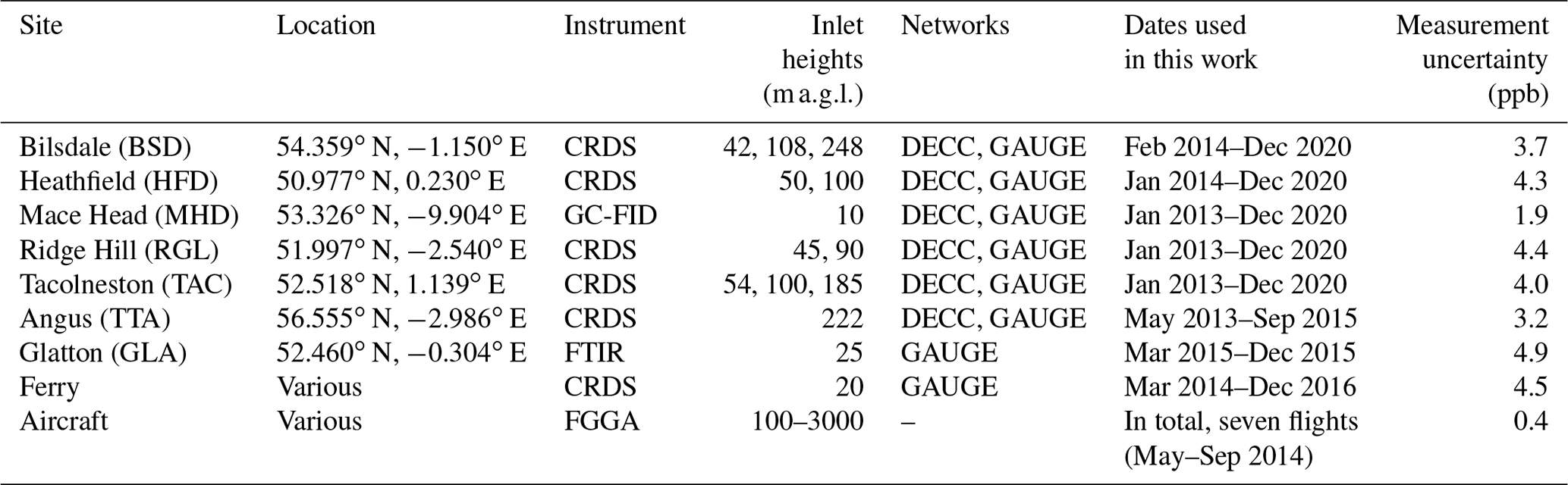
Methane observations for this study were taken from the following six tower sites across the UK and ROI: Mace Head, the Republic of Ireland (MHD), Ridge Hill, England (RGL), Tacolneston, England (TAC), Angus, Scotland (TTA), Bilsdale, England (BSD), and Heathfield, England (HFD). The locations of the measurement sites, instrumentation and time period covered are given in Table 1.
With the exception of MHD, CH4 mole fractions were measured at each tall tower site using a Picarro cavity ring-down spectroscopy (CRDS) instrument. These measurements were calibrated using dry air standards in aluminium cylinders on the World Meteorological Organization (WMO)-2004A scale. Methane measurements at MHD were made using a gas chromatograph and flame ionization detector (GC-FID) every 40 min. Calibration of the GC-FID measurements on the Tohoku University scale was performed using wet-filled standards in electropolished stainless steel cylinders (Ganesan et al., 2015; Prinn et al., 2018a). To ensure consistency between the two calibration scales, observations from the five sites calibrated on the WMO-2004A scale were multiplied by a factor of 1.0003 (Dlugokencky et al., 2005). For tower sites with more than one inlet (BSD, HFD, RGL and TAC), measurements from the highest inlet were used in this study in an attempt to reduce the impact of local influences on the posterior emission estimates. For the purposes of this work, observational uncertainties were defined as being the variability of 1 min mole fraction measurements in each observational period used in the inverse modelling (4 h). Values are shown in Table 1.
2.2 Additional GAUGE measurements
As part of the GAUGE project, CH4 data from an additional short-term measurement site in Glatton (GLA), Cambridgeshire, were also collected. These measurements were made on top of a 25 m high church tower using a Fourier transform infrared spectroscopy (FTIR) instrument and calibrated on the WMO-2004A scale (Palmer et al., 2018). Information on the instrumentation, inlet heights and data availability from each site is detailed in Table 1. We define the addition of this site and the shipborne data outlined below to the DECC tower network as the GAUGE network.
Table 1Location, inlets, instruments, network definitions, sampling dates and observational uncertainties of each measurement site. Note: ppb – parts per billion; CRDS – cavity ring-down spectroscopy; FGGA – fast greenhouse gas analyser; FTIR – Fourier transform infrared; GC-FID – gas chromatograph and flame ionization detector.
2.2.1 Ship-based measurements
As part of the GAUGE project, CH4 measurements were taken on board a DFDS Seaways commercial freight ferry serving a route between Rosyth, Scotland, and Zeebrugge, Belgium. Return journeys were completed 3 times a week, with the ship charting a course just off the east coast of the UK for much of its journey, providing a regular transect of England and southern Scotland (Fig. 1). Measurements from the Zeebrugge–Rosyth ferry were made on a Picarro CRDS system and calibrated on the WMO-2004A calibration scale. Measurements were taken from the bow of the ship. Further details on the measurement set-up and calibration are given in Helfter et al. (2019). Data from times when the ferry was in, or within, 50 km of either port were discarded due to the likely proximity of anthropogenic sources which would be unresolved at the resolution of the transport model output.
2.2.2 Aircraft
CH4 measurements were taken on board the UK's FAAM (Facility for Airborne Atmospheric Measurements) BAe 146 research aircraft, using a Los Gatos fast greenhouse gas analyser (FGGA) instrument (O'Shea et al., 2013; Pitt et al., 2019). Continuous CH4 measurements were made in conjunction with altitude, longitude and latitude coordinates. Measurements were calibrated on the WMO-2004A calibration scale, with calibrations performed on an hourly basis during flights. As part of the GAUGE project, a number of flights were conducted with a variety of flight paths, including orbits of the British Isles to more dense trajectories upwind and downwind of London (Palmer et al., 2018). In this study, we used data from seven of these flights, over the course of four different months, between May and September 2014 (see Fig. 1).
3.1 NAME
The Numerical Atmospheric-dispersion Modelling Environment (NAME; Jones et al., 2007; Manning et al., 2011) was used to calculate the relationship between the emissions field and simulated mole fractions. The set-up for calculating this relationship at each of the sites followed that described in Manning et al. (2011) and Lunt et al. (2016). Model particles were released from each inlet height ± 20 m in the model and tracked backwards in time for 30 d. The integrated residence time of the particles in the layer adjacent to the surface (0 to 40 m a.g.l.) was output on a latitudinal–longitudinal grid to give a direct measure of the sensitivity of mole fractions to changes in surface emissions from each grid cell. This grid had a resolution of , equating to an approximate 25 km resolution. The NAME computational domain covered 10.7–79.1∘ N and −97.9–39.4∘ E. Annual mean (2015) NAME sensitivity footprints over NW Europe from each of the measurement sites are shown in Fig. 1.
NAME was driven by offline meteorology fields from the UK Met Office's Unified Model (UM; Cullen, 1993). The simulations used meteorology from a UK-specific mesoscale product at 1.5 km horizontal resolution (UKV) and 1 h temporal resolution, nested within the model's global fields (UMG). The vertical structure of the mesoscale fields contained 57 levels, up to a maximum height of 12 km, with 16 levels resolved in the lowest 1 km. The mesoscale meteorology was nested within the model's global meteorology fields, which were at an approximate horizontal resolution of 25 km up to July 2014, then 17 km until July 2017 and 12 km thereafter. The global fields contained 59 vertical levels up to a maximum height of 29 km, with approximately 11 levels in the lowest 1 km. The temporal resolution of the global fields was 3 h.
The UKV fields only cover a latitudinal–longitudinal area not much bigger than the UK. As a result of this, and as a consequence of the larger computational burden of running at high resolution, a number of changes were made to the default NAME set-up, as described in Lunt et al. (2016). The UKV meteorology was used to drive the transport of the particles within the UKV area for the first 3 d after their release. Once particles left the UKV area, further transport was dictated by the UMG meteorology, and similarly, after 3 d, only the UMG meteorology was then available to transport the particles, regardless of location. The temporal dependence was applied to make the runs more computationally efficient, and sensitivity tests showed that there was no significant difference between having the UKV fields available for the full 30 d back-trajectory or only the first 3 d (since most particles will leave the limited UKV area within the 3 d period). Although NAME was run at the higher resolution of the UKV meteorology, the footprints were still output on the same grid to ensure a regular grid structure throughout the domain.
3.2 GEOS-Chem
A second set of model simulations were performed for 2015 using the GEOS-Chem model (Turner et al., 2015). The model was run in a nested configuration, driven by meteorology from the GEOS-FP fields at . The nested European domain covered 40–62∘ N and 15∘ W–15∘ E. Boundary conditions of this European domain were informed by a consistent global simulation of the model at . The global simulation was driven by prior emissions from the Emissions Database for Global Atmospheric Research (EDGAR) v4.3.2 for anthropogenic sources, the WetCHARTs v1.0 database for wetlands (Bloom et al., 2017) and the Global Fire Emissions Database (GFED) v4s for biomass burning (van der Werf et al., 2017). The nested run used the same prior emissions field as for the NAME inversions, with the UK NAEI distribution for the UK and EDGAR in all other countries. Sensitivities of the atmospheric measurements to emissions were calculated using GEOS-Chem from 26 basis function regions in the European domain, with 14 of these for the UK and ROI. Emission sensitivities were calculated from each region by perturbing 2-monthly emissions from each one independently. Each emissions perturbation was represented by a different tagged tracer within the model. The model was sampled at the location and height of the DECC network measurement inlets, and the difference in modelled mole fraction due to each basis function perturbation was calculated. For each basis function, emissions were turned off after 2 months, and the tracer concentrations were tracked for a further 10 d, by which time the difference in concentrations at the measurement sites due to the perturbations had decreased to zero. The corresponding tracer outputs were used to build up the sensitivity matrix describing the change in modelled CH4 mole fraction given a change in emissions. The emissions regions used are shown in the Supplement (Fig. S1). Sensitivities were also calculated to the magnitude of the global boundary condition fields at each of the four domain boundaries, and the uncertainty in these fields explored in the inversion.
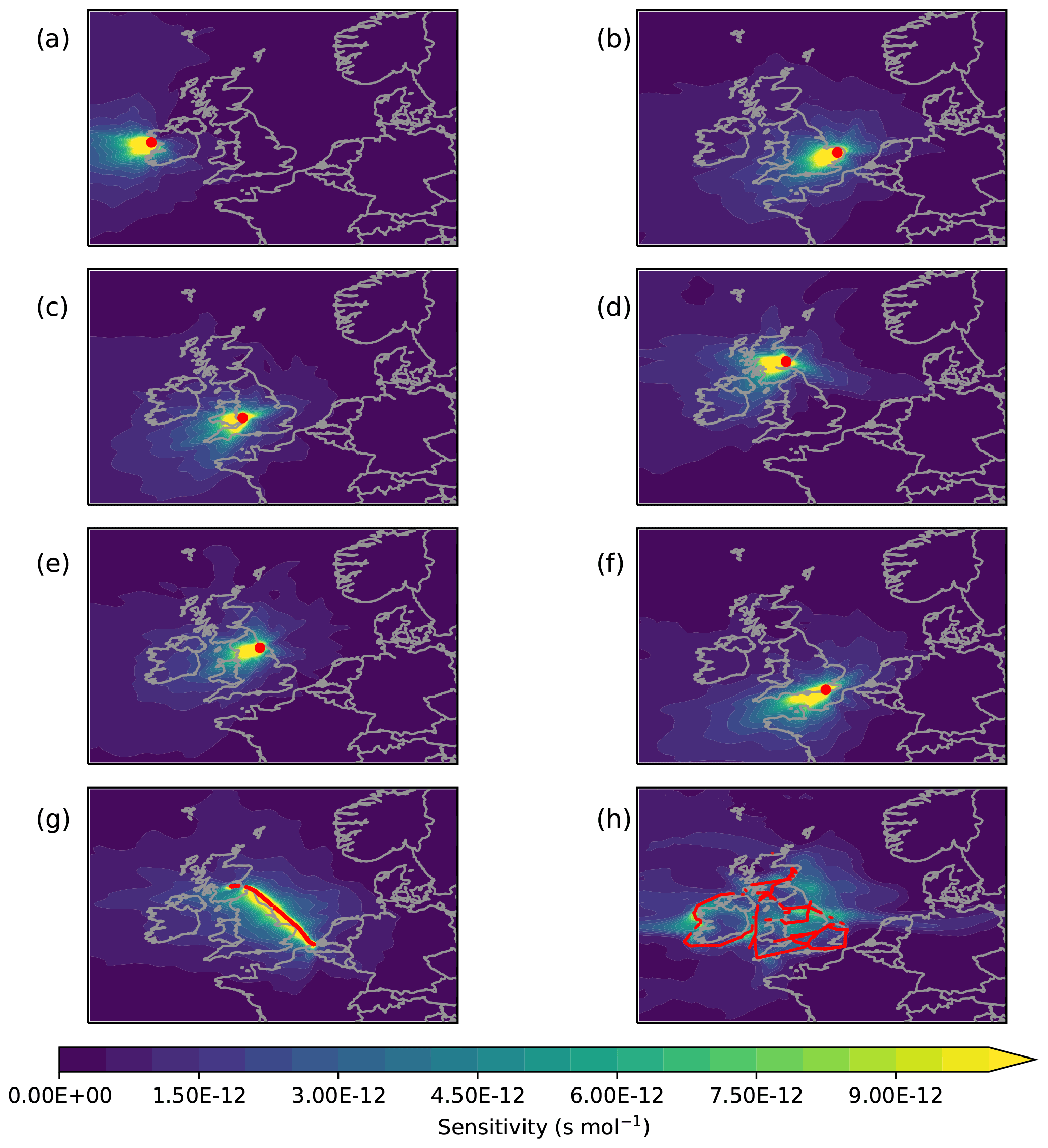
Figure 1Annual mean NAME footprints for each of the measurement sites in 2015, showing the areas the measurements are most sensitive to (the overall NAME domain extended much wider). (a) MHD, (b) TAC, (c) RGL, (d) TTA, (e) BSD, (f) HFD, (g) ferry and (h) FAAM aircraft. Data for the FAAM aircraft (seven flights) are from 2014. Red dots show the measurement locations. The domain shown covers the spatially varying domain used in the rj-mcmc inversions, which is a subset of the full NAME inversion domain.
The prior emissions spatial distribution was combined from several different sources for the inversions in this study. Emissions from the UK (and the surrounding ocean) were distributed according to the spatial distribution given by the UK's NAEI from 2015 (NAEI2015; available at http://naei.beis.gov.uk/data/, last access: 21 March 2021). These maps are provided for total anthropogenic emissions and individual source sectors on an approximate 1×1 km resolution grid. Outside of the UK, emissions were distributed according to the EDGAR v4.3.2 inventory, which provides the emissions distribution at resolution, regridded to the resolution of the NAME output. Figure 2 shows the spatial distribution of the NAEI2015 prior, along with the breakdown of the three main NAEI2015 source sectors in the UK, i.e. agriculture, waste and energy. Emissions from the agriculture sector are primarily concentrated in the western parts of the country, with emissions from livestock being the main source. Waste and energy emissions are more concentrated around urban areas. In addition to the anthropogenic sources, there is likely a small natural component of methane emissions from the UK associated primarily with methanogenesis in peatlands. These natural emissions were not accounted for in the NAEI2015 prior, and owing to the uncertainty over the exact spatial distribution, magnitude and temporal variation in these natural emissions, we ignore this relatively minor component of emissions in our prior emissions estimate. However, the main use of peatlands in the UK is for livestock grazing, and thus, the areas where these emissions are expected to emanate are already accounted for in the spatial distribution of the prior. The inversion set-up allows for the emissions from these regions to change in the inversion, if required. We acknowledge that the lack of a natural emissions component may lead to our estimates of anthropogenic UK methane emissions being slightly overestimated but explore the impact of the spatial distribution of prior emissions in Sect. 6.5. The same spatial prior was used for all years and months in our inversions, ensuring zero trend in the prior over the study period.

Figure 2Maps showing the spatial distribution of the NAEI emissions in the UK at 5×5 km resolution, showing the (a) agriculture sector, (b) waste sector, (c) energy sector and (d) the total anthropogenic source.
Inversions were performed using two separate methodologies. Unless stated otherwise, the majority of inversions were performed using the reversible jump Markov chain Monte Carlo (rj-mcmc) method, described in Lunt et al. (2016) and briefly summarized below. A further set of inversions were performed using the Inversion Technique for Emission Modelling (InTEM), which is the UK Met Office's inversion modelling system, and it is described in Sect. 5.2.
5.1 Reversible-jump MCMC (rj-mcmc)
The rj-mcmc method (Green, 1995) is an extension of traditional Metropolis–Hastings MCMC (Metropolis et al., 1953; Hastings, 1970). The inversion method explores prior probability density functions (PDFs) of a set of parameters and updates estimates of these PDFs based on atmospheric data. In this work, the parameters describe emissions and terms describing boundary conditions. Each PDF is defined by a set of hyper-parameters that describe the form of the PDF, such as the mean and standard deviation. MCMC methods allow the flexibility to use any PDF without needing to impose Gaussian distributions, allowing emissions parameters to be defined as positive only through the use of a lognormal distribution. In the rj-mcmc method, in addition to exploring the PDF of the parameters (and hyper-parameters describing those PDFs), the number of unknowns is itself treated as an unknown. The method can take the uncertainty inherent in the aggregation of basis functions into account, providing a more robust estimate of the posterior parameters PDF. The rj-mcmc method can be applied to basis functions in one- and two-dimensional problems in an effort to avoid making restrictive assumptions about the discretization of parameter space (Sambridge et al., 2013). In this work, the basis functions describe 2D spatial regions over which each parameter value applies (defined herein as a region). Starting from some prior PDF of parameters, the MCMC algorithm works by sampling from the target distribution of each parameter or hyper-parameter after it has been informed by the data. The PDFs are explored by perturbing the current state of the parameters model, m, at each step of the chain to a new state, m′. In the rj-mcmc algorithm, this perturbation is chosen from one of the following proposals:
-
update the parameter's vector and prior hyper-parameters
-
add a new region (birth)
-
remove a region (death)
-
move a region (move)
-
update a model–measurement covariance hyper-parameter.
If the perturbation is favourable, then the parameters model will move to the new state, m′, or otherwise will remain unchanged. Whether a proposal is favourable or not depends on a combination of the ratio of prior, proposal and likelihood probabilities of the current and proposed model. The prior probability, ρ(m), describes how likely a particular model state is based on the form of the a priori PDF, and the ratio gives the relative prior probabilities of the new and current model state. The likelihood ratio, , relates the relative probabilities of predicting the data given the new and current model states. The proposal ratio, , describes the probability of picking the new model state from the current one and vice versa. The proposal is accepted, provided the following equation is satisfied:
where U is a uniformly distributed random number between 0 and 1. Strictly speaking, there is an additional term, a Jacobian matrix, J, that should be taken into account for the dimension changing proposals. However, in the birth–death approach used here, where the new dimension is one less or one more than the current state, this term is always 1 and so can be ignored. The acceptance criteria help to ensure efficiency in sampling the target distribution since unfavourable regions are rejected. Through exploring many thousands of samples, an estimate of the posterior distribution is reached.
The rj-mcmc algorithm was run for 200 000 iterations after a burn-in period of 50 000 iterations, and the chain thinned to store every 100th iteration, giving 2000 stored samples of the posterior distribution. During the burn-in, tuning of the jump sizes for the parameters and hyper-parameter proposals was performed in order to achieve acceptance ratios of between 20 % and 50 % to ensure efficient exploration of the chain (Tarantola, 2005).
Unlike the parameter and hyper-parameter proposals, there is no natural analogue of the jump size for the birth, death and move steps since the acceptance ratio is more heavily dependent on the location of the proposed change as opposed to the value. However, while reasonable acceptance ratios were reported in Lunt et al. (2016), these were primarily due to the outer regions of the domain being relatively unconstrained by the data, leading to higher overall acceptance ratios. By contrast, birth, death and move proposals in regions of high sensitivity had lower acceptance ratios. To improve the efficiency of the algorithm, the upper limit for the number of regions was set to 150 as a means of limiting the amount of time spent exploring regions in poorly constrained parts of the domain.
The rj-mcmc methodology was applied following the methodology in Lunt et al. (2016), where the basis functions each described a 2D spatial region with an unknown number of these 2D spatial regions. The PDF for the number and location of spatial regions was set to be uniform and allowed to vary between 5 and 150, with a starting number of 50. Independent 2-monthly inversions were performed, with emissions assumed to be constant over each 2-month period. To improve the computational efficiency and minimize time spent exploring regions of little impact on the data, the spatially varying domain was restricted to 45–61∘ N and −12.5–15∘ E. The extent of this region is shown in Fig. 1. Outside of the spatially varying sub-domain, there were six fixed regional basis functions describing emissions from regions between the edge of the sub-domain and the edge of the full NAME computational domain.
In addition to the contribution from emissions, the CH4 mole fractions are comprised of the underlying background variations. To estimate this background contribution in the rj-mcmc inversion, information on where the NAME particles left the NAME domain was stored to give an estimate of the sensitivity of the measurements to the mole fractions at the boundaries of the domain. These sensitivities were then combined with a climatology of mole fraction curtains from the global Eulerian Model for Ozone and Related chemical Tracers (MOZART; Emmons et al., 2010) to give an estimate of the baseline mole fractions at each site. The MOZART mole fractions were generated using gridded emissions estimates from various methane sources, including anthropogenic emissions from the Emissions Database for Global Atmospheric Research (EDGAR v4.3.2; Janssens-Maenhout et al., 2011), biomass burning (van der Werf et al., 2017), natural wetlands (Bloom et al., 2012) and other sources (Fung et al., 1991), as described in Lunt et al. (2016). These unconstrained MOZART-generated curtains provided a prior estimate of the boundary condition mole fractions which were updated alongside emissions in the inversion. Optimized posterior mean model estimates of these baseline mole fractions at each site are included in Figs. S2–S15.
Using a hierarchical Bayesian approach (described in Ganesan et al., 2014), uncertainty parameters were themselves estimated in the inversion with the prior emissions uncertainty and model–measurement uncertainty each described by a PDF. The prior uncertainty on each spatial emissions basis function was set to 50 % but described by a log-normal PDF, which itself had a standard deviation of 50 %, which was explored in the inversion. The model–measurement uncertainty was split into a fixed observational uncertainty and a variable model uncertainty. The observational uncertainty was defined as the variability in the observations in each 4 h measurement period, as shown in Table 1. The prior model uncertainty was described by a Gaussian PDF, which had a mean of 20 ppb and standard deviation of 8 ppb. Different values for model uncertainty were estimated for each site every 7 d. The correlation length scale, relating the covariance in time between measurement errors, was fixed at 6 h. The inversion, using sensitivities calculated using GEOS-Chem, followed a similar hierarchical MCMC approach. However, due to the computational complexity of calculating grid cell sensitivities with this Eulerian model, these inversions used a fixed basis function definition and, thus, did not include the reversible jump component of births, deaths and move proposals.
5.2 InTEM
The Inversion Technique for Emission Modelling (InTEM; Manning et al., 2011; Arnold et al., 2018) has been developed over many years and is the model used annually to estimate UK emissions of greenhouse gases in the UK national inventory report (Brown et al., 2020) submitted to the UNFCCC. InTEM is a Bayesian inversion system and assumes all errors are Gaussian but uses a non-negative least squares solver (Lawson and Hanson, 1974), preventing any negative solutions from being found.
InTEM uses the same NAME sensitivity footprints as used in the rj-mcmc inversions. The prior information comes from the following two sources: the first is the spatial distribution of CH4 emissions as used in the rj-mcmc, namely UK NAEI2015 nested inside EDGAR FT2010. The second is from an estimate of the time-varying boundary mole fractions of methane. The latter is derived from CH4 observations at Mace Head during times identified as being representative of the well-mixed Northern Hemisphere baseline, namely times when the air has travelled predominately from northern Canada with low influence from populated regions, high altitudes, local sources or southerly latitudes. A fourth-order polynomial is fitted to these data over a rolling 6-month window, and a daily baseline uncertainty is estimated based on the root mean square of the fit.
InTEM allows the prior baseline to be adjusted based on 11 directional and height values, depending on where the air enters the NAME-modelled domain, as described in Arnold et al. (2018). The inversion also allows for a site-specific bias adjustment to be made. The geographical grid used in the inversion is dependent on the sensitivity of the area to the observations; the higher the sensitivity, the higher the resolution of the grid up to the native resolution of the NAME output, as described in Manning et al. (2011), and the magnitude of the prior emissions from each area. In addition, the size of each grid area is limited to predefined country boundaries. The model–observation uncertainty applied to the data varies for each 4 h period and is comprised of three elements, i.e. observational uncertainty, baseline uncertainty and a meteorological uncertainty. Observational uncertainty is estimated from the variability in the observations in the 4 h period and baseline uncertainty is discussed above. The third element of uncertainty is proportional to the magnitude of the simulated pollution event (10 %), with a minimum uncertainty defined as the annual median CH4 pollution event for each site (Manning et al., 2021).
5.3 Observation selection
Inverse methodologies generally assume that all observational and modelling errors are unbiased and random. Such a situation may not occur at certain times of the day or under particular meteorological conditions. These might include times under particularly stable planetary boundary layers (PBLs), where small errors in vertical mixing parameterizations could lead to significant errors in atmospheric trace gas distributions or due to miscalculation of modelled PBL height related to surface temperature and nighttime surface heat balance. A common approach to negate potential model biases is to use only observations from the middle of the day (e.g. Peters et al., 2010; Bergamaschi et al., 2015). However, this approach has the disadvantage of ignoring the majority of the available data, and there is no guarantee that both the real and model atmosphere are similarly well mixed. Indeed, this well-mixed criterion may only be appropriate during summer when the boundary layer stability tends to exhibit a pronounced diurnal cycle. However, it may not be met in the afternoon during winter months in particularly stable conditions. Conversely, potentially well-modelled data points may be excluded if they fall outside of this acceptable time window.
An alternative approach is to filter the data based on meteorological considerations. In this approach, the atmospheric transport model is assumed to perform poorly under certain conditions such as stable boundary layers and low wind speeds, where unresolved sub-grid-scale processes (e.g. sea breezes) or parameterized processes (e.g. convection) may dominate in reality but not in the model.
We followed this approach through the use of a number of data filters, which differed slightly between InTEM and rj-mcmc inversions. In the rj-mcmc inversions, for sites with more than one inlet height (BSD, HFD, RGL and TAC) we only used data from times when the difference between mole fractions recorded at different heights within the same hour was less than 10 ppb. This threshold was set to attempt to limit data to those times when the air was well-mixed. Since multiple inlets were not available at all sites, we further limited data use to times when the NAME simulated boundary layer height was greater than the measurement inlet height plus 250 m, and the local contribution of the 25 grid cells surrounding each measurement site to the NAME footprint was smaller than 10 % of the total footprint. These three filters were designed to maximize the probability of only including well-mixed air masses in our analysis and resulted in approximately 40 %–60 % of available data being discarded for the rj-mcmc inversions, depending on the measurement site. InTEM inversions followed a similar set-up but used a threshold of 20 ppb for the difference in CH4 mole fraction between different inlet heights and a fixed boundary layer height limit of 300 m. InTEM inversions discarded fewer observations that rj-mcmc, removing between 30 % for MHD to 45 % for the majority of other sites. A plot of the mean number of observations per 2-month inversion period at each site from the respective inversion approaches is included in Fig. S16.
6.1 UK and ROI emissions estimates (2013–2020)
UK and ROI CH4 emissions are presented for the 8-year period from January 2013 to December 2020, inclusive, from the rj-mcmc and the InTEM inversions. Independent 2-monthly inversions were performed using data from all available tall tower sites and the MHD baseline station in each month. This varied from only three sites in early 2013 to all six sites in 2014 and 2015 and five sites during 2016–2020. All uncertainties from the rj-mcmc inversions represent the 95 % confidence interval, which is given by the 2.5th and 97.5th percentiles of the posterior distribution. Uncertainties from the InTEM inversions represent 2σ standard deviations from the mean.
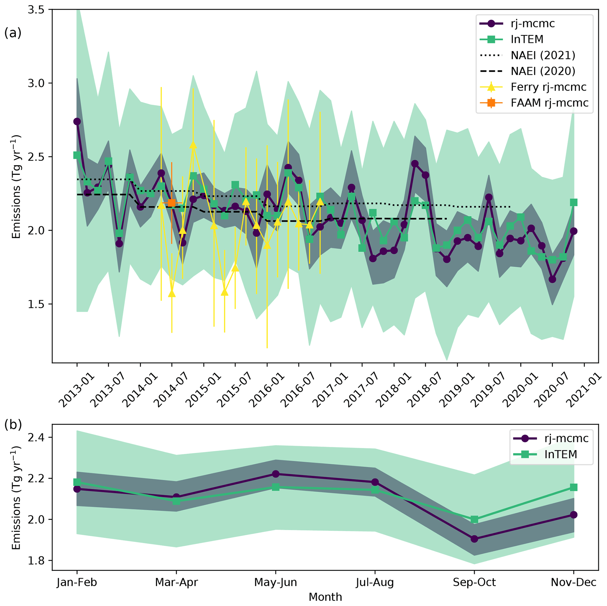
Figure 3(a) Time series of 2-monthly UK emissions from the two inversion methods, showing the rj-mcmc spatially varying inversion (purple) and InTEM inversion (green). The rj-mcmc results are also included from the mobile measurement platforms of the ferry (yellow) and the FAAM aircraft (orange). The solid lines and markers designate the means, while the shading and uncertainty bars show the 95 % confidence intervals of the posterior distributions. Black dashes show the NAEI annual mean from the two most recent reports (NAEI2020 and NAEI2021). (b) The mean seasonal cycle of 2-month mean emissions from the full network inversions between 2013 and 2020.
Figure 3 shows the time series of derived posterior UK CH4 emissions from the two different inversion set-ups. The two methods result in similar estimates of UK emissions, with a mean annual UK estimate from the rj-mcmc spatial inversion of 2.10 (2.01–2.18) and 2.12 (1.86–2.38) Tg yr−1 from InTEM. Due to the different treatment of model–measurement uncertainties in the inversions, the InTEM posterior emissions estimates have much larger confidence intervals. Over the 8-year inversion period (2013–2020), the annual emissions estimates from rj-mcmc show a negative trend of Tg yr−2 (p=0.006). The trend is calculated via least squares regression accounting for the emission uncertainties. InTEM results have a similar negative trend of Tg yr−2, although, due to the larger uncertainties, this is not statistically significant (p=0.2). The rj-mcmc trend is equivalent to a 2 % decrease each year and broadly consistent with the estimated decrease in the NAEI of −0.03 Tg yr−2.
Emissions estimates for 2020 were 1.89 (1.81–1.97) and 1.93 (1.70–2.16) Tg yr−1 from the rj-mcmc and InTEM inversions, respectively. These estimates are in line with the trend in emissions from previous years and do not indicate any substantial response to the national lockdowns enforced as a result of the coronavirus pandemic. Given the dominance of agriculture and waste sectors in UK CH4 emissions, which are unlikely to have been impacted by the events of 2020, this finding is not unexpected. Plots of the changing posterior emission distributions over time from the rj-mcmc and InTEM inversions are included in Figs. S17–S18.
The estimated mean emissions between 2013 and 2018, from both inversions of 2.16 (2.07–2.24) and 2.17 (1.91–2.44) Tg yr−1 rj-mcmc and InTEM, respectively, are similar to the NAEI2020 reported emissions of 2.13 Tg yr−1. However, in 2021, the inventory was revised to include a larger contribution of emissions from the land use, land use change and forestry (LULUCF) sector. These are estimated to contribute 0.19 Tg yr−1 to the UK total emissions and largely account for the difference between the NAEI2021 and NAEI2020 reported emissions shown in Fig. 3. The revised NAEI2021 emissions have a mean of 2.23 Tg yr−1 between 2013 and 2019, with a near-constant offset compared to the previous year's submission.
It should be noted that the prior emissions used in the inversion (NAEI2015) ignored any potential contribution from natural emissions to the UK total, in common with previous versions of the NAEI. Within the additional LULUCF emissions added in the 2021 inventory, the majority of CH4 emissions are split between grasslands (50 %) and wetlands (42 %). This type of land is mostly used for stock grazing (Brown et al., 2020), and as such, it is likely that any wetland emissions would be spatially indistinguishable from agricultural emissions in those parts of the country where these land types are prevalent. Thus, while natural emissions are not explicitly accounted for in the prior, it is unlikely that significant emissions would occur in areas where the prior does not already account for agricultural emissions. The sensitivity to the prior emissions distribution is explored in Sect. 6.5.
6.1.1 Seasonal emissions cycle
The bottom panel of Fig. 3 shows the seasonal cycle of the UK emissions derived from both inversions. The InTEM inversion results do not show a large seasonal cycle, while the rj-mcmc results find the highest emissions on average during May–August. This is consistent with the period of highest surface temperature in the UK. Although the rj-mcmc observation selection criteria result in a larger seasonal cycle of observations used than InTEM (see Fig. S16), the difference in respective seasonal emission cycles cannot be easily explained by this difference. The greatest number of observations in the rj-mcmc inversions are used in July–August and the fewest in November–December, whereas the rj-mcmc emission estimates are greatest in May–June and smallest in September–October.
The results shown in Fig. 3 represent the total methane emissions from the UK and do not distinguish between different emissions sources. We divide these total CH4 emissions into the respective sector contributions by assuming that the relative proportion of the NAEI sector split within each grid cell is correct but that the total magnitude is uncertain. Using the spatial distribution of the posterior estimates from the rj-mcmc inversion, we find that the summertime peak is most likely due to emissions from the agriculture sector. Posterior agriculture emissions during May–August are 0.14 Tg yr−1 greater than during other times of year, compared to 0.05 Tg yr−1 greater emissions from waste and 0.01 Tg yr−1 smaller emissions in the energy sector. This finding is qualitatively similar to that of Pison et al. (2018), who estimated a similar summertime peak in agriculture emissions from France. As noted above, the overlap in the spatial distributions of the agricultural and LULUCF emissions means that the estimated seasonal cycle from the agriculture sector could instead reflect changes in grassland or wetland emissions. Indeed, the presence of a summertime peak in European CH4 emissions estimates has previously been interpreted as evidence for the role of natural wetland CH4 emissions across Europe (Bergamaschi et al., 2018). While the most recent version of the NAEI (2021) explicitly accounts for grassland and wetland emissions under the LULUCF category, spatial mapping of this distribution is not currently available, thus preventing a direct comparison. There is a notable positive emissions anomaly in the rj-mcmc estimates (and, to a lesser extent, in InTEM) during the summer of 2018. Compared to mean summer emissions, both inversions show a mean positive anomaly of 0.2 Tg yr−1 in 2018. In June–August 2018, the UK average temperatures were 1.4 ∘C above the 1981–2010 seasonal average, and rainfall was 73 % of the long-term seasonal average (data from https://www.metoffice.gov.uk/research/climate/maps-and-data/summaries/index, last access: 28 June 2021). Both inversions show enhanced emissions across much of the UK in summer 2018, with no one specific region responsible (see Fig. S19).
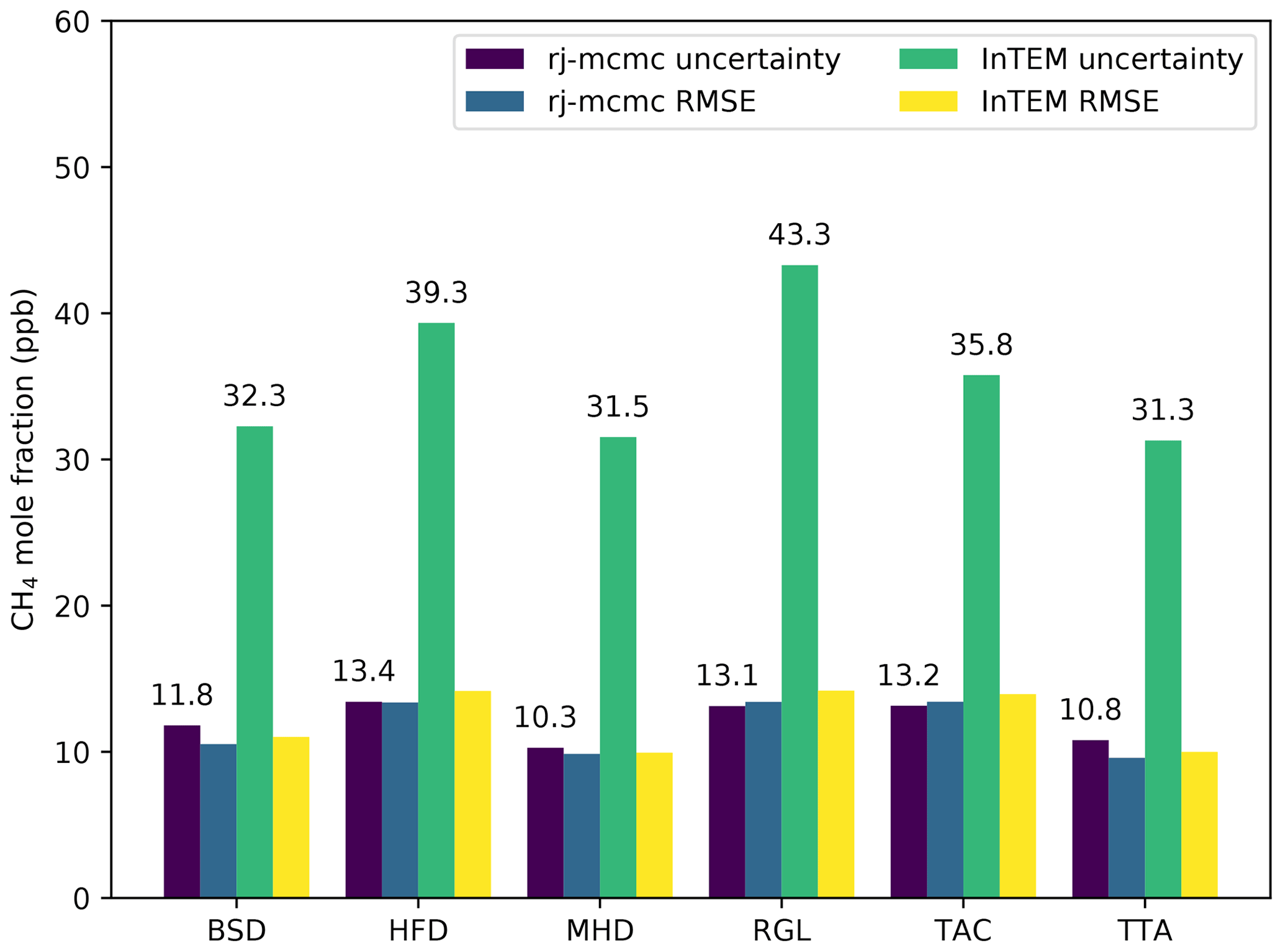
Figure 4Mean posterior model–measurement uncertainties at each site from the rj-mcmc inversions and prescribed uncertainties in the InTEM inversions. Also shown are the mean posterior root mean square errors (RMSE) from the respective inversions. BSD – Bilsdale; HFD – Heathfield; MHD – Mace Head; RGL – Ridge Hill; TAC – Tacolneston; TTA – Angus.
6.1.2 Uncertainty comparison
Figure 4 shows the mean posterior estimates of the model–measurement uncertainty at each site from the rj-mcmc inversions and the prescribed uncertainties from the InTEM inversion. The results show that the rj-mcmc posterior model–measurement uncertainties are, on average, around 3 times smaller than those used in the InTEM inversions. Figure 4 shows the rj-mcmc model–measurement uncertainties are more consistent with the posterior fit to the data at each site, as demonstrated through the root mean square error (RMSE) at each site. Therefore, the posterior emission uncertainties of the rj-mcmc inversion may be more representative of the emissions uncertainty, if uncertainties are dominated by non-systematic components. As a result, we concentrate the majority of our remaining analysis on the results of the rj-mcmc inversion rather than InTEM. The 3 times larger model–measurement uncertainty used in the InTEM inversions helps to explain the much larger posterior emission uncertainties, which are 3.5 times larger on average.
Posterior model–measurement uncertainties are smallest at those sites that are furthest removed from local sources. These include Bilsdale, Mace Head and Angus. Both Bilsdale and Angus inlets are over 200 m, whereas Mace Head is a background station. In contrast, the Ridge Hill, Tacolneston and Heathfield sites have lower measurement inlet heights and are closer to large CH4 sources. These features are also reflected in the InTEM uncertainties, albeit with larger values.
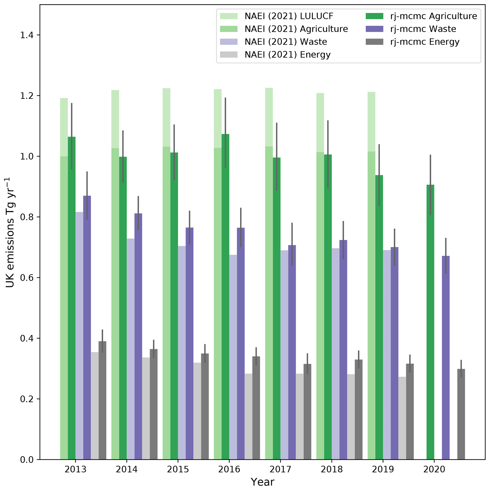
Figure 5Annual UK emission estimates for agriculture and LULUCF (green), waste (purple) and energy (grey) sectors. The lighter shade in each colour represents the NAEI value, while the darker shade shows the average posterior distribution from the rj-mcmc inversion. Uncertainty bars represent the 95 % confidence interval. Sector totals are calculated by scaling the individual prior sector distributions by the total posterior scale factor of each grid box. The rj-mcmc sector breakdown does not include an explicit representation of LULUCF.
6.1.3 Sector emissions
Figure 5 shows the annual mean sector emissions from the rj-mcmc inversion alongside the annual estimates from the 2021 inventory report. In common with the NAEI (2021), the agriculture section was found to have the largest emissions, with a mean, over the 2013–2019 period, of 1.01 (0.91–1.11) Tg yr−1 compared to the NAEI average of 1.02 Tg yr−1. The waste estimates were similar to the NAEI average of 0.71 Tg yr−1 at 0.76 (0.69–0.82) Tg yr−1. Emissions from the energy and industrial processes sectors were estimated to be 0.34 (0.31–0.37) Tg yr−1 compared to the NAEI mean of 0.30 Tg yr−1.
The largest component of the negative trend in the rj-mcmc UK total emissions are from the waste and energy sectors, at −0.05 ± 0.01 and −0.02 ± 0.01 Tg yr−2, respectively (p<0.01). Agriculture does not display a significant trend, in common with the NAEI. We stress that the NAEI trends are not included in the prior emissions used in the inversions, so the trends found in the posterior emissions estimates are independent of the NAEI reported trends. Pearson correlation coefficients between the sectors from the inversions are 0.6 between agriculture and waste, 0.4 between agriculture and energy and 0.7 between waste and energy. These correlation coefficients indicate some influence of the changes in one distribution on any other. This may be due to overlap in the spatial distribution of each sector and the natural parsimony of the Bayesian solution, which favours broad-scale regional changes over finer resolution updates.
Posterior annual mean emissions estimates for ROI from the rj-mcmc inversion are shown in Fig. 6 and averaged 0.66 (0.61–0.72) Tg yr−1 between 2013 and 2020. This compares to ROI's national inventory report average of 0.56 Tg yr−1. We do not find any substantial trend in the annual mean rj-mcmc ROI estimates. The posterior estimates do show a reasonably large seasonal cycle, with emissions greatest during May–August and 20 % greater than emissions between November–February. The largest contributor to ROI's reported CH4 emissions is the agriculture sector which accounts for 90 % of reported national emissions. Similarly to the UK, the larger summertime emissions could, therefore, be representative of a summertime peak in agricultural emissions or an indication of seasonal variation in natural wetland or grassland emissions.
6.2 Devolved administration emissions
The UK is composed of its four devolved administrations (DAs) of England, Scotland, Wales and Northern Ireland (NI), with a separate part of the NAEI prepared for each. We compare the rj-mcmc results for each DA to establish consistency with the DA inventories and the degree to which these are independently resolved. Due to delays in the production of the DA inventories relative to the UK national inventory, we use the NAEI DA values from the 2020 report (NAEI2020).
Figure 6 shows the annual mean rj-mcmc and InTEM emissions from each of the DAs alongside the corresponding NAEI2020 estimates and emissions estimates from ROI. NAEI2020 leaves a portion of emissions from the North Sea as being unallocated to any DA, which we assign here to Scotland to be consistent with the inversion outputs. The rj-mcmc posterior emissions estimates are consistent with NAEI2020 for each DA. We find the largest mean emissions from England of 1.48 (1.36–1.61) Tg yr−1 between 2013–2018 compared to 1.42 Tg yr−1 in NAEI2020 during the same period. InTEM results for England have a mean emissions of 1.48 (1.17–1.79) Tg yr−1 between 2013–2018. The rj-mcmc posterior estimates from England display a negative trend of −0.05 ±0.01 Tg yr−2, accounting for the negative trend found in the total UK estimates.
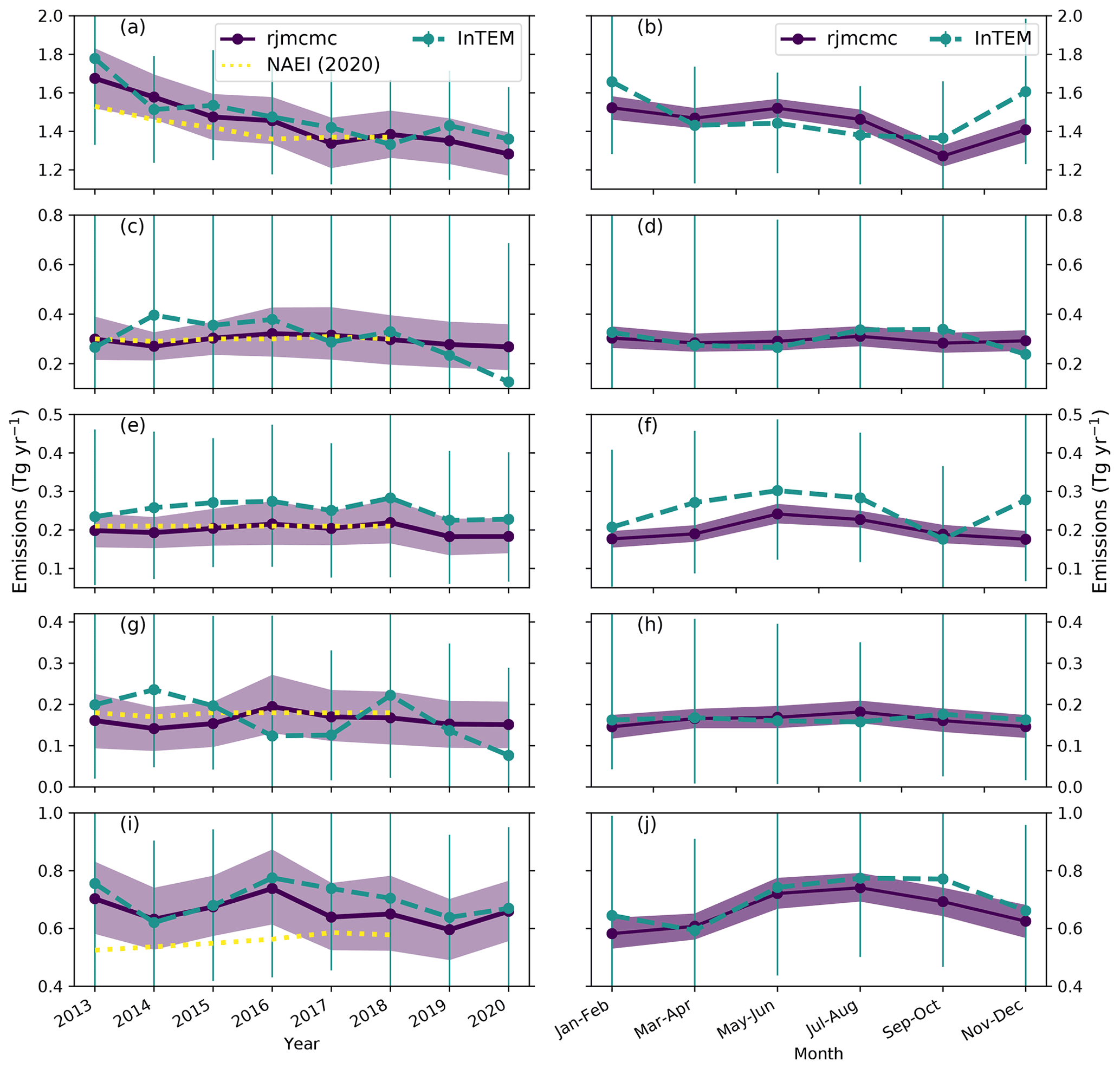
Figure 6Annual emission estimates and seasonal cycles for the individual devolved administrations (DAs) of the UK and estimates for ROI. The figure shows (a) the rj-mcmc and InTEM annual mean estimates for England, (b) the mean seasonal cycle for England from rj-mcmc and InTEM, (c–d) Scotland, (e–f) Wales, (g–h) Northern Ireland (NI) and (i–j) the Republic of Ireland. The shading and error bars represent the 95 % confidence intervals. Dotted lines represent the DA NAEI estimates from the 2020 inventory report, except for ROI, which represent the country's national inventory total.
Posterior rj-mcmc estimates for the other DAs are largely flat and consistent, with no negative trend in NAEI2020. Similarly, from InTEM, there are no significant trends, although even the trend from England (−0.05 ± 0.01 Tg yr−2) is not significant (p=0.5) due to the large posterior uncertainties. As discussed in Sect. 6.1.2, these are likely an overestimate of the true uncertainties due to random model errors. For this reason, we restrict further discussion of inversion results to the rj-mcmc inversions. We find small correlation coefficients for each 2-month rj-mcmc inversion between the different DAs of between −0.05 and 0.08, indicating that the posterior DA totals are independent of each other, and the atmospheric observation network provides an ability to independently resolve emissions from these sub-national regions of the order of 104 to 105 km2.
Posterior 95 % confidence intervals as a percentage of the annual means are of the order of 15 %–20 % for England, 40 %–65 % for Scotland, 40 %–50 % for Wales and 70 %–80 % for Northern Ireland. We note that the annual mean uncertainty on the Scotland estimate increased from 40 % to 65 % after 2015 following the decommissioning of the tall tower measurement site in Angus, Scotland (TTA). Of the remaining five sites, four are located in England, which, along with the larger mean emissions, are the likely cause of the smaller uncertainties for England.
Figure 6 also shows the mean seasonal cycle of rj-mcmc emissions from each DA. Similar to ROI, we find a May–August peak in emissions from Wales and Northern Ireland that is 20 %–30 % greater than winter emissions. The NAEI reports 70 % and 80 % of emissions from agriculture from Wales and Northern Ireland, respectively, which could explain the summertime peak. Emissions from England and Scotland do not display a similar seasonal cycle, although we find a consistent dip in emissions from England during September–October.
6.3 Measurement network configuration comparison
In this section, we investigate the impact that the volume and type of data used has on the UK rj-mcmc emissions estimates. The results presented in Sect. 6.1 used all available tall tower sites of the DECC network (although the exact number of stations varied from three to six, depending on the year and month). Here, we investigate how the UK means, uncertainties and trends are affected by the number of available measurement sites. We investigated how the emissions estimates are affected by using only one background site (MHD) or using one site regularly intercepting pollution peaks (TAC). We test the impact of using these two sites in combination, using two sites regularly intercepting pollution events (RGL and TAC) and through the use of two separate mobile measurement platforms.
Table 2Comparison of posterior rj-mcmc emissions from different measurement networks in 2015. All units in are given in teragrams per year (Tg yr−1) unless stated otherwise. DECC = BSD-HFD-MHD-RGL-TAC-TTA. GAUGE = DECC + GLA + ferry .
n/a: not applicable.
Table 2 shows the 2015 annual mean posterior UK emissions that are estimated from these networks, together with the NAEI2020 and the 2013–2020 emissions trend. The results show the annual mean posterior uncertainties are over 3 times larger when using the single background site compared to using all available tower sites. However, using just TAC data leads to a 70 % drop in the posterior uncertainty, with a slight further gain in combining the information of two measurement sites. The two-site network of MHD-TAC can constrain annual UK CH4 emissions to within a 95 % confidence range of 0.24 Tg, compared to 0.15 Tg when using all available sites.
The 95 % uncertainty range on the UK's NAEI reported total for 2018 is 0.68 Tg. On this basis, the MHD-only inversion provides no uncertainty reduction, whereas both the two-site network inversions provide at least a 50 % reduction on this 95 % range. Of course, the inversion accounts only for random uncertainties and likely underestimates the total uncertainty due to ignoring systematic errors. Even so, with only two measurement sites, emissions are constrained to within a range of less than 15 %. We find that a negative trend in UK CH4 emissions is undetectable on an 8-year timescale in the MHD-only inversion but is detected in both the two-site inversions in addition to the DECC network inversion. At the regional level, we find correlation coefficients of less than 0.1 between most of the different DAs in both two-site inversions. The 95 % confidence range for England in 2015 decreases from 0.87 Tg for MHD only to 0.21 Tg for TAC only, 0.19 Tg for both two-site inversions and 0.11 Tg for the full six sites. This shows that the TAC site on its own provides a large part of the constraint on England emissions. This is due to the site's sensitivity to regions of southern England that contain a large proportion of the UK's emissions (see Fig. 1b). The advantage of having multiple sites is more evident when attempting to estimate sector emissions. For the two-site inversion of MHD–TAC, we find a 10 % increase in correlations between different posterior sector distributions. We also find that the estimated trends in waste and energy sector emissions are no longer statistically significant (p>0.15).
Figure 7 shows the spatial distribution of posterior uncertainty for some of the different networks. Low uncertainty values over most of southern and central England are seen when using TAC data alongside MHD, providing much greater constraint compared to just MHD. A similar feature is seen for Wales, where most of the uncertainty reduction comes from the addition of one or both of RGL and TAC. For Scotland, most constraint comes from the TTA site in the DECC network. The results show, perhaps predictably, that measurement sites within a region (or downwind of emissions from a region) provide the greatest uncertainty reduction of emissions within that region. The addition of the TAC site to MHD is enough to constrain both the UK and England emissions to within a 95 % confidence range of 0.25 Tg yr−1. The additional sites of the DECC network increase confidence on regional emission estimates, but the annual means are similar and, they add little additional constraint on the total UK estimate and trend due to the concentration of the majority of emissions in central and southern England.

Figure 7Posterior 95 % confidence interval for 2015 as a fraction of the posterior estimate for each grid box. Darker colours indicate regions of lower uncertainty. Maps are shown for the following different measurement networks: (a) MHD, (b) MHD–TAC, (c) DECC network, (d) GAUGE network (DECC + GLA + ferry), (e) ferry and (f) FAAM aircraft (2014). Gold dots indicate locations of measurements used. The plot extent is not indicative of the inversion domain.
6.3.1 Mobile platforms and GAUGE network
Figure 3 and Table 2 also contain rj-mcmc estimates from the two mobile measurement sites. FAAM results are from 2014, covering seven flights, one each in both May and June, two in July and three in September 2014. The FAAM inversion was run using data averaged into 5 min periods. The FAAM emissions estimate of 2.19 (1.91–2.46) Tg yr−1, shown in Fig. 3, is consistent with both the rj-mcmc and InTEM estimates from the DECC network. As a sensitivity test, a smaller averaging time of 1 min was tested and resulted in a UK estimate of 1.76 (1.52–2.00) Tg yr−1 that was inconsistent with other networks. It is possible that data recorded at the timescale of 1 min was not representative of the NAME model grid cells. The trade-off from averaging into periods of 5 min was a large reduction in data volume and, hence, larger posterior uncertainties. Figure 7f shows the very limited area in which the posterior emissions uncertainty is small when using this platform. To constrain national scale fluxes to the same degree as the two-site networks on either 2-monthly or annual timescales, it would be necessary to perform a much larger number of flights than the seven used here in the absence of continuous surface data.
Posterior rj-mcmc emissions for 2015 derived from the ferry are slightly smaller than from the DECC network, primarily due to England's emissions being smaller, but still overlap within the 95 % confidence range. The 2-monthly emissions estimates from the ferry data have larger uncertainties than from the DECC network rj-mcmc inversions and greater seasonal variability, as shown in Fig. 3. Nevertheless, the UK mean over the full sampling period of 2014–2016 was 2.02 (1.88–2.18) Tg yr−1, more consistent with the DECC network mean over the same period of 2.16 (2.12–2.22) Tg yr−1. Helfter et al. (2019) estimated a UK and ROI emissions rate of 2.55 ± 0.48 Tg yr−1 from the same shipborne data between 2015 and 2017, using a mass balance approach. The estimate included ROI due to the use of the MHD site as the measure of inflow for the mass balance calculations. Adding the ROI component of our posterior emissions estimate to the UK gives 2.59 (2.37–2.84) Tg yr−1, helping to reconcile these estimates. However, as shown in Fig. 7, the shipborne posterior uncertainty estimates are lowest over eastern parts of the UK and show little constraint over western parts and ROI.
Finally, we combined all available ground-based data together in 2015, incorporating the six sites of the DECC tower network plus the shipborne measurements and additional data from a church tower in Glatton, Cambridgeshire (GLA). We did not include the aircraft data due to the limited days of sampling concentrated in 2014. We find similar UK CH4 emissions compared to the DECC tower network of 2.12 (2.05–2.19) Tg yr−1 in 2015, with no substantial changes in emission estimates for any of the DAs or ROI. Ostensibly, this can be explained by the additional data of GLA and the ferry providing constraints on regions, such as southern England, that are already well sampled by the other measurement data. The value of the additional data is likely, instead, to lie in analysing smaller-scale variations that are beyond the focus of this work.
6.4 Atmospheric transport model comparison
Figure 8 shows a comparison of UK, ROI and DA emissions estimated using NAME rj-mcmc and a second transport model, GEOS-Chem, during 2015. The figure shows similar estimates of total UK emissions in each 2-month period, with estimates overlapping within the 95 % confidence level. The 2015 mean UK estimate using GEOS-Chem was 2.08 (2.00–2.16) Tg yr−1 compared to 2.14 (2.06–2.21) Tg yr−1 from NAME. The 2-monthly estimates overlap within the range of the posterior uncertainties, with the greatest difference for emissions from England. The 95 % confidence range of each 2-month estimate from GEOS-Chem is 25 % larger than from NAME, possibly due to a reduced ability to fit the data. The NAME inversions have a mean bias-corrected RMSE between the observations and modelled mole fractions averaged across all sites of 10 ppb, compared to 22 ppb from the GEOS-Chem inversions. This RMSE for GEOS-Chem is fairly uniform across sites, with a range of 19.6–22.9 ppb. Similarly, the mean posterior model–measurement error from the GEOS-Chem inversions was 18 ppb across all sites, which is 50 % larger than the mean uncertainty of 12 ppb for NAME rj-mcmc inversions.
Although the UK annual estimates are similar, the results show that the atmospheric transport model and inversion set-up have a larger impact on the DA emissions and at sub-annual timescales. The GEOS-Chem inversion resolved only 14 independent basis functions for UK emissions in each 2-month period and 26 in total across the European inversion domain. The number of basis functions varied in the NAME rj-mcmc inversions, and are difficult to isolate to the UK alone, but averaged 113 across the inversion domain. Despite these differences, the UK annual mean estimates are similar, and both are slightly smaller than the 2.25 Tg assumed in the prior. A fuller comparison of the differences between transport models is beyond the scope of this work. However, our results suggest that the annual UK emissions estimated are not exclusive to the use of NAME. Improving the spatial resolution of GEOS-Chem basis functions, by including a greater number of unknowns, may help to reconcile differences at the sub-national scale and improve the fit of the GEOS-Chem posterior modelled mole fractions with the data.

Figure 8The 2-monthly posterior estimates for 2015 from NAME (blue) and GEOS-Chem (green) inversions, and the prior used for the inversions (black dash). The panels show estimated emissions for (a) the UK, (b) England, (c) Scotland, (d) Wales, (e) Northern Ireland (NI) and (f) the Republic of Ireland. Shading represents the 95 % confidence range of the inversion estimates.
6.5 Prior estimate comparison
The impact of the prior distribution of emissions was tested by using two further prior emission distributions. First, we considered the case of using the EDGAR distribution of emissions over the UK instead of the NAEI. The EDGAR UK mean emissions are 30 % larger than the NAEI at 2.92 Tg yr−1. This allows us to investigate the impact of a potentially significant bias in the prior on the ability to maintain a consistent constraint on UK emissions. A second prior distribution assumed a flat rate of emissions throughout all land-based areas of Europe. For the purposes of this flat prior, emissions from the sea were considered to be negligible, and the annual mean UK emissions were 2.34 Tg yr−1, although, due to the relative areas of the different DAs, emissions from England were 23 % smaller than the NAEI and almost 2.5 times larger from Scotland.
Figure 9 shows the annual mean emissions estimated for the UK, and devolved administrations using these different priors, in addition to the main results. The annual mean estimates from both the EDGAR and flat prior inversions are larger than the main estimate, with limited to no overlap within the 95 % confidence intervals. The annual mean emissions rates were 2.24 (2.15–2.33) Tg yr−1 and 2.37 (2.25–2.49) Tg yr−1 for the EDGAR and flat inversions, respectively. The mean estimates of the EDGAR and flat inversions are 0.14 and 0.27 Tg greater than our main results.
In both inversions, the main reason for the difference in UK emissions is due to differences in Scotland. Both EDGAR and flat priors were larger than the NAEI in Scotland by 0.08 and 0.45 Tg, respectively. This is reflected in the average annual mean posterior estimates of 0.36 (0.32–0.42) Tg yr−1 and 0.53 (0.44–0.61) Tg yr−1 from the respective inversions, compared to 0.29 (0.25–0.34) Tg yr−1 from the main results. The flat prior inversion in particular maintains an offset in the posterior of 0.24 Tg that does not overlap within the range of the posterior uncertainties, indicating a lack of constraint on Scotland's emissions. The posterior corrections to both EDGAR and flat priors are broadly consistent with the spatial differences between the NAEI distribution and the respective priors. The differences in the flat prior inversion are particularly smooth but still show the largest positive differences between posterior and prior in central England, and negative differences in northern Scotland, similar to the NAEI (see Fig. S20).

Figure 9Annual mean emissions between 2013 and 2020 for inversions using different prior distributions from the NAEI (purple), EDGAR (blue) and a flat distribution (green). Estimates are shown for (a) the UK, (b) England, (c) Scotland, (d) Wales, (e) Northern Ireland (NI) and (f) the Republic of Ireland. Shading represents the 95 % confidence interval. Dashed lines represent the magnitudes of the respective priors.
The spatial distribution of Scotland's emissions in the flat prior inversion is likely to be particularly unrealistic compared to other parts of the UK, due to the presence of substantial emissions in areas such as the sparsely populated Scottish highlands. Nevertheless, the results show that the atmospheric network is unable to correct for this likely error in the priors. This shortcoming of the measurement network is evident both before and after the decommissioning of the one measurement site (TTA) in Scotland, reflecting a lack of sensitivity to the northernmost part of the UK.
The results shown in Fig. 9 demonstrate that the posterior emissions estimate from England is relatively robust to assumptions about the prior distribution and magnitude. All inversions estimate mean emissions for England of around 1.5 Tg yr−1 and a negative trend of −0.05 Tg yr−1, despite the prior means ranging from 77 %–140 % of the NAEI value. England's emissions account for around 70 % of the UK total in the main results. The prior sensitivity tests demonstrate an independence on the distribution and magnitude of the prior for the majority of emissions.
A similar result is found for a two-site measurement network using measurements from only MHD and TAC (see Fig. S21). Emissions estimated for England from this two-site network and the NAEI prior are 1.47 (1.37–1.58) Tg yr−1 compared to 1.44 (1.38–1.50) Tg yr−1 from the full measurement network. The annual emissions estimates for England have a trend of −0.04 ± 0.02 Tg yr−2. When using the EDGAR prior and just MHD–TAC data, a similar mean of 1.50 (1.38–1.61) Tg yr−1 is found and a trend of −0.04 ± 0.02 Tg yr−2. With the flat prior, the mean emissions are 1.38 (1.28–1.48) Tg yr−1, and the trend −0.03 ± 0.02 Tg yr−2. Although the results display larger differences than the full network, the majority of England's, and thus the UK's, emissions are relatively well constrained by this two-site network and overlap within the 95 % uncertainty range. However, greater differences between inversions using different priors are found for the other DAs when using only the two-site network, highlighting the importance of the denser measurement network for more robust evaluation of all the UK's CH4 emissions.
We show how the UK's CH4 emissions can be evaluated from a network of tall-tower sites over the 8-year period of 2013–2020. Using a network of six measurement sites and a hierarchical Bayesian inversion method, emissions can be constrained to a 95 % confidence interval that is within ± 10 % of the mean value on a 2-month timescale. A trend of −0.05 ± 0.01 Tg yr−2 in the annual means is detectable by the network over the 7-year period. We find a similar negative trend of −0.06 ± 0.04 Tg yr−2 using a second inversion method (InTEM).
We show that similar results are achieved using a network of only two sites, with a 95 % confidence interval of ± 10 % and a trend of −0.03 Tg yr−1. The results imply that, for constraining UK annual CH4 emissions, a two-site network is sufficient, although this is somewhat dependent on the non-uniform distribution of emissions across the country. Although this work focuses on CH4, this result may have relevance for some synthetic greenhouse gases such as certain hydrofluorocarbons (HFCs). In the UK and ROI, these are measured only at MHD and TAC. Our results suggest that the addition of further instruments at other sites would not significantly change conclusions on the comparison with the NAEI for these gases (e.g. Manning et al., 2021), assuming that the majority of emissions are within England. Although spatial distributions of HFCs may be more uncertain for gases used in refrigeration and mobile air-conditioning systems such as HFC-134a, this assumption should hold due to the population distribution of the UK.
At the level of devolved administrations, even when using the full measurement network, our results for Scotland are shown to be dependent on the prior emissions distribution. The current network has insufficient sensitivity to the northernmost parts of the UK. Our prior sensitivity tests show that the prior definition of emissions in this region carries over into the posterior estimates, with estimates not overlapping within the estimated uncertainties. This may not be overly significant for an assessment of anthropogenic CH4, where sources in (sparsely populated) northern Scotland are thought to be minimal. However, for assessing natural sources such as wetland CH4 or biospheric CO2, this may be a more significant shortcoming.
The TTA site was decommissioned in late 2015, and there have been no measurements in Scotland since then as part of the UK's monitoring network. However, even when TTA data were available, there was no convergence in the inversion estimates for Scotland from using different prior distributions. This is due to a lack of sensitivity to the northernmost parts of Scotland and also the North Sea, where there are significant oil- and gas-related emissions. To fully constrain emissions from the northernmost parts of the UK, measurements with greater sensitivity to both of these areas would be required. For England and Wales, we find the posterior estimates were not overly influenced by the magnitude or spatial distribution of the prior, as evidenced through sensitivity tests using the EDGAR distribution or a flat distribution of emissions.
The rj-mcmc inversion method solves for bulk CH4 emissions, relying on the posterior scaling of the prior distribution to split the total CH4 emissions into individual sectors. We find the higher emissions of summertime to be most likely due to the agriculture sector emissions, and the negative trend in annual emissions is most likely due to decreases in the waste and energy sectors. This second finding is in common with the NAEI, despite no trends being built into our priors. However, due to the lack of spatial independence in the prior distributions and the natural parsimony of the rj-mcmc inversion method, we find positive correlations of 0.4–0.7 in our posterior sector estimates. Solving independently for the three main sector emissions could reduce this interdependence, although the same issue is likely to remain. Alternatively, the use of a co-tracer, such as ethane, or direct measurements of the δ13C ratio may help to isolate emissions from the energy sector in particular.
This work has focused on an evaluation of the UK's methane emissions and national emissions verification. We find, for the UK (≈ 2×10⁵ km2), a network of two in situ measurement sites (sensitive to around 70 % of national total emissions) is sufficient to constrain emissions at the national scale to within a 95 % confidence range of around 10 %. Additional measurement sites are required to reduce the posterior uncertainties on national and sub-national emissions and to better constrain trends both nationally and from different regions and emission sectors. Finally, we note that while the UK NAEI is prepared with a delay of 2 years, the atmospheric measurement emissions estimation can be carried out with a delay of, at most, a few months. This efficiency offers a potential advantage for using atmospheric measurements to track the UK's progress towards greenhouse gas emissions reduction targets.
Tower data from the UK DECC network are available at https://catalogue.ceda.ac.uk/uuid/f5b38d1654d84b03ba79060746541e4f (O'Doherty and Say, 2020). MHD data can be accessed from the AGAGE archive at http://cdiac.ess-dive.lbl.gov/ndps/alegage.html (Prinn et al., 2018b). Aircraft, ferry and GLA data from the GAUGE project can be accessed at http://catalogue.ceda.ac.uk/uuid/9a1295858ff14fc6acea73e356a8842c (GAUGE project team, 2015).
The supplement related to this article is available online at: https://doi.org/10.5194/acp-21-16257-2021-supplement.
MFL conducted the rj-mcmc inversions, GEOS-Chem simulations and wrote the paper. AJM conducted the NAME simulations and InTEM inversions. AJM and MR contributed to the writing of the paper. All other authors contributed data collection, calibration, analysis and quality control and provided comments on the paper.
Anita Ganesan is editor of ACP.
Publisher’s note: Copernicus Publications remains neutral with regard to jurisdictional claims in published maps and institutional affiliations.
University of Edinburgh and University of Manchester authors were supported by grants from the Natural Environment Research Council (NERC). Paul I. Palmer gratefully acknowledges funding from the National Centre for Earth Observation, funded by NERC. University of Bristol authors were supported by the UK Department for Business Energy and Industrial Strategy and NERC. Since 2017, measurements at Heathfield have been maintained by the National Physical Laboratory, mainly under funding from the National Measurement System.
This research has been supported by the Natural Environment Research Council (grant nos. NE/K002449/1, NE/S003819/1, NE/I027282/1, NE/M014851/1, NE/L013088/1, NE/K002236/1, NE/S004211/1, NE/N016548/1, NE/V00963X/1, NE/K00221X/1 and NE/R016518/1).
This paper was edited by Christoph Gerbig and reviewed by two anonymous referees.
Arnold, T., Manning, A. J., Kim, J., Li, S., Webster, H., Thomson, D., Mühle, J., Weiss, R. F., Park, S., and O'Doherty, S.: Inverse modelling of CF4 and NF3 emissions in East Asia, Atmos. Chem. Phys., 18, 13305–13320, https://doi.org/10.5194/acp-18-13305-2018, 2018. a, b
Bergamaschi, P., Krol, M., Meirink, J. F., Dentener, F., Segers, A., van Aardenne, J., Monni, S., Vermeulen, A. T., Schmidt, M., Ramonet, M., Yver, C., Meinhardt, F., Nisbet, E. G., Fisher, R. E., O'Doherty, S., and Dlugokencky, E. J.: Inverse modeling of European CH4 emissions 2001–2006, J. Geophys. Res.-Atmos., 115, D22309, https://doi.org/10.1029/2010JD014180, 2010. a
Bergamaschi, P., Corazza, M., Karstens, U., Athanassiadou, M., Thompson, R. L., Pison, I., Manning, A. J., Bousquet, P., Segers, A., Vermeulen, A. T., Janssens-Maenhout, G., Schmidt, M., Ramonet, M., Meinhardt, F., Aalto, T., Haszpra, L., Moncrieff, J., Popa, M. E., Lowry, D., Steinbacher, M., Jordan, A., O'Doherty, S., Piacentino, S., and Dlugokencky, E.: Top-down estimates of European CH4 and N2O emissions based on four different inverse models, Atmos. Chem. Phys., 15, 715–736, https://doi.org/10.5194/acp-15-715-2015, 2015. a, b
Bergamaschi, P., Karstens, U., Manning, A. J., Saunois, M., Tsuruta, A., Berchet, A., Vermeulen, A. T., Arnold, T., Janssens-Maenhout, G., Hammer, S., Levin, I., Schmidt, M., Ramonet, M., Lopez, M., Lavric, J., Aalto, T., Chen, H., Feist, D. G., Gerbig, C., Haszpra, L., Hermansen, O., Manca, G., Moncrieff, J., Meinhardt, F., Necki, J., Galkowski, M., O'Doherty, S., Paramonova, N., Scheeren, H. A., Steinbacher, M., and Dlugokencky, E.: Inverse modelling of European CH4 emissions during 2006–2012 using different inverse models and reassessed atmospheric observations, Atmos. Chem. Phys., 18, 901–920, https://doi.org/10.5194/acp-18-901-2018, 2018. a, b
Bloom, A. A., Palmer, P. I., Fraser, A., and Reay, D. S.: Seasonal variability of tropical wetland CH4 emissions: the role of the methanogen-available carbon pool, Biogeosciences, 9, 2821–2830, https://doi.org/10.5194/bg-9-2821-2012, 2012. a
Bloom, A. A., Bowman, K. W., Lee, M., Turner, A. J., Schroeder, R., Worden, J. R., Weidner, R., McDonald, K. C., and Jacob, D. J.: A global wetland methane emissions and uncertainty dataset for atmospheric chemical transport models (WetCHARTs version 1.0), Geosci. Model Dev., 10, 2141–2156, https://doi.org/10.5194/gmd-10-2141-2017, 2017. a
Brown, P., Cardenas, L., Choudrie, S., Jones, L., Karagianni, E., MacCarthy, J., Passant, N., Richmond, B., Smith, H., Thistlethwaite, G., Thomson, A., Turtle, L., and Wakeling, D.: UK Greenhouse Gas Inventory, 1990 to 2018, Annual report for submission under the framework convention on climate change, Tech. rep., Department for Business Energy and Indusrial Strategy (BEIS), 2020. a, b, c
Brown, P., Cardenas, L., Choudrie, S., Del Vento, S., Karagianni, E., MacCarthy, J., Mullen, P., Passant, N., Richmond, B., Smith, H., Thistlethwaite, G., Thomson, A., Turtle, L., and Wakeling, D.: UK Greenhouse Gas Inventory, 1990 to 2019, Annual report for submission under the framework convention on climate change, Tech. rep., Department for Business Energy and Indusrial Strategy (BEIS), 2021. a
Brunner, D., Arnold, T., Henne, S., Manning, A., Thompson, R. L., Maione, M., O'Doherty, S., and Reimann, S.: Comparison of four inverse modelling systems applied to the estimation of HFC-125, HFC-134a, and SF6 emissions over Europe, Atmos. Chem. Phys., 17, 10651–10674, https://doi.org/10.5194/acp-17-10651-2017, 2017. a
Cullen, M. J. P.: The Unified Forecast Climate Model, Meteorol. Mag., 122, 81–94, 1993. a
Dlugokencky, E. J., Myers, R. C., Lang, P. M., Masarie, K. A., Crotwell, A. M., Thoning, K. W., Hall, B. D., Elkins, J. W., and Steele, L. P.: Conversion of NOAA atmospheric dry air CH4 mole fractions to a gravimetrically prepared standard scale, J. Geophys. Res.-Atmos., 110, D18306, https://doi.org/10.1029/2005JD006035, 2005. a
Emmons, L. K., Walters, S., Hess, P. G., Lamarque, J.-F., Pfister, G. G., Fillmore, D., Granier, C., Guenther, A., Kinnison, D., Laepple, T., Orlando, J., Tie, X., Tyndall, G., Wiedinmyer, C., Baughcum, S. L., and Kloster, S.: Description and evaluation of the Model for Ozone and Related chemical Tracers, version 4 (MOZART-4), Geosci. Model Dev., 3, 43–67, https://doi.org/10.5194/gmd-3-43-2010, 2010. a
Fung, I., John, J., Lerner, J., Matthews, E., Prather, M., Steele, L. P., and Fraser, P. J.: Three-dimensional model synthesis of the global methane cycle, J. Geophys. Res., 96, 13033, https://doi.org/10.1029/91jd01247, 1991. a
Ganesan, A. L., Rigby, M., Zammit-Mangion, A., Manning, A. J., Prinn, R. G., Fraser, P. J., Harth, C. M., Kim, K.-R., Krummel, P. B., Li, S., Mühle, J., O'Doherty, S. J., Park, S., Salameh, P. K., Steele, L. P., and Weiss, R. F.: Characterization of uncertainties in atmospheric trace gas inversions using hierarchical Bayesian methods, Atmos. Chem. Phys., 14, 3855–3864, https://doi.org/10.5194/acp-14-3855-2014, 2014. a
Ganesan, A. L., Manning, A. J., Grant, A., Young, D., Oram, D. E., Sturges, W. T., Moncrieff, J. B., and O'Doherty, S.: Quantifying methane and nitrous oxide emissions from the UK and Ireland using a national-scale monitoring network, Atmos. Chem. Phys., 15, 6393–6406, https://doi.org/10.5194/acp-15-6393-2015, 2015. a, b, c, d
GAUGE project team: GAUGE (Greenhouse gAs UK and Global Emissions) project: Ground based and airborne atmospheric measurement data collection, Centre for Environmental Data Analysis [data set], available at: http://catalogue.ceda.ac.uk/uuid/9a1295858ff14fc6acea73e356a8842c (last access: 2 November 2021), 2015. a
Green, P. J.: Reversible jump Markov chain Monte Carlo computation and Bayesian model determination, Biometrika, 82, 711–732, 1995. a
Hastings, W. K.: Monte-Carlo Sampling Methods Using Markov Chains and Their Applications, Biometrika, 57, 97–101, 1970. a
Helfter, C., Mullinger, N., Vieno, M., O'Doherty, S., Ramonet, M., Palmer, P. I., and Nemitz, E.: Country-scale greenhouse gas budgets using shipborne measurements: a case study for the UK and Ireland, Atmos. Chem. Phys., 19, 3043–3063, https://doi.org/10.5194/acp-19-3043-2019, 2019. a, b, c
Henne, S., Brunner, D., Oney, B., Leuenberger, M., Eugster, W., Bamberger, I., Meinhardt, F., Steinbacher, M., and Emmenegger, L.: Validation of the Swiss methane emission inventory by atmospheric observations and inverse modelling, Atmos. Chem. Phys., 16, 3683–3710, https://doi.org/10.5194/acp-16-3683-2016, 2016. a
IPCC: 2006 IPCC Guidelines for National Greenhouse Gas Inventories, Prepared by the National Greenhouse Gas Inventories Programme, edited by: Eggleston, H. S., Buendia, L., Miwa, K., Ngara, T., and Tanabe, K., IGES, Japan, 2006. a
Janssens-Maenhout, G., Crippa, M., Guizzardi, D., Muntean, M., and Schaaf, E.: Emissions Database for Global Atmospheric Research, version v4.3.2 part I Greenhouse gases (gridmaps), European Commission, Joint Research Centre (JRC) [Dataset] PID, available at: http://data.europa.eu/89h/jrc-edgar-edgar_v432_ghg_gridmaps (last access: 2 November 2021), 2017. a
Jeong, S., Hsu, Y. K., Andrews, A. E., Bianco, L., Vaca, P., Wilczak, J. M., and Fischer, M. L.: A multitower measurement network estimate of California's methane emissions, J. Geophys. Res.-Atmos., 118, 11339–11351, 2013. a
Jones, A., Thomson, D., Hort, M., and Devenish, B.: The UK Met Office's next-generation atmospheric dispersion model, NAME III, Air Pollution Modeling and Its Applications XVII, 17, 580–589, 2007. a
Lawson, C. and Hanson, R.: Solving Least Squares Problems, Solving Least Squares Problems, Prentice-Hall, Englewood Cliffs, NJ, 1974. a
Lunt, M. F., Rigby, M., Ganesan, A. L., and Manning, A. J.: Estimation of trace gas fluxes with objectively determined basis functions using reversible-jump Markov chain Monte Carlo, Geosci. Model Dev., 9, 3213–3229, https://doi.org/10.5194/gmd-9-3213-2016, 2016. a, b, c, d, e, f
Manning, A. J., O'Doherty, S., Jones, A. R., Simmonds, P. G., and Derwent, R. G.: Estimating UK methane and nitrous oxide emissions from 1990 to 2007 using an inversion modeling approach, J. Geophys. Res.-Atmos., 116, D02305, https://doi.org/10.1029/2010jd014763, 2011. a, b, c, d
Manning, A. J., Redington, A. L., Say, D., O'Doherty, S., Young, D., Simmonds, P. G., Vollmer, M. K., Mühle, J., Arduini, J., Spain, G., Wisher, A., Maione, M., Schuck, T. J., Stanley, K., Reimann, S., Engel, A., Krummel, P. B., Fraser, P. J., Harth, C. M., Salameh, P. K., Weiss, R. F., Gluckman, R., Brown, P. N., Watterson, J. D., and Arnold, T.: Evidence of a recent decline in UK emissions of hydrofluorocarbons determined by the InTEM inverse model and atmospheric measurements, Atmos. Chem. Phys., 21, 12739–12755, https://doi.org/10.5194/acp-21-12739-2021, 2021. a, b
Metropolis, N., Rosenbluth, A. W., Rosenbluth, M. N., Teller, A. H., and Teller, E.: Equation of State Calculations by Fast Computing Machines, J. Chem. Phys., 21, 1087–1092, 1953. a
Myhre, G., Shindell, D., Bréon, F.-M., Collins, W., Fuglestvedt, J., Huang, J., Koch, D., Lamarque, J.-F., Lee, D., Mendoza, B., Nakajima, T., Robock, A., Stephens, G., Takemura, T., and Zhang, H.: Anthropogenic and Natural Radiative Forcing In: Climate Change 2013: The Physical Science Basis. Contribution of Working Group I to the Fifth Assessment Report of the Intergovernmental Panel on Climate Change, chap. 8, Cambridge University Press, Cambridge, United Kingdom and Ney York, NY, USA, 659–740, 2013. a
O'Doherty, S. and Say, D.: UK DECC (Deriving Emissions linked to Climate Change) Network, Centre for Environmental Data Analysis [data set], available at: http://catalogue.ceda.ac.uk/uuid/f5b38d1654d84b03ba79060746541e4f (last access: 2 November 2021), 2020. a
Oney, B., Henne, S., Gruber, N., Leuenberger, M., Bamberger, I., Eugster, W., and Brunner, D.: The CarboCount CH sites: characterization of a dense greenhouse gas observation network, Atmos. Chem. Phys., 15, 11147–11164, https://doi.org/10.5194/acp-15-11147-2015, 2015. a
O'Shea, S. J., Bauguitte, S. J.-B., Gallagher, M. W., Lowry, D., and Percival, C. J.: Development of a cavity-enhanced absorption spectrometer for airborne measurements of CH4 and CO2, Atmos. Meas. Tech., 6, 1095–1109, https://doi.org/10.5194/amt-6-1095-2013, 2013. a
Palmer, P. I., O'Doherty, S., Allen, G., Bower, K., Bösch, H., Chipperfield, M. P., Connors, S., Dhomse, S., Feng, L., Finch, D. P., Gallagher, M. W., Gloor, E., Gonzi, S., Harris, N. R. P., Helfter, C., Humpage, N., Kerridge, B., Knappett, D., Jones, R. L., Breton, M. L., Lunt, M. F., Manning, A. J., Matthiesen, S., Muller, J. B. A., Mullinger, N., Nemitz, E., O'Shea, S., Parker, R. J., Percival, C. J., Pitt, J., Riddick, S. N., Rigby, M., Sembhi, H., Siddans, R., Skelton, R. L., Smith, P., Sonderfeld, H., Stanley, K., Stavert, A. R., Wenger, A., White, E., Wilson, C., and Young, D.: A measurement-based verification framework for UK greenhouse gas emissions: an overview of the Greenhouse gAs Uk and Global Emissions (GAUGE) project, Atmos. Chem. Phys., 18, 11753–11777, https://doi.org/10.5194/acp-18-11753-2018, 2018. a, b, c
Peters, W., Krol, M. C., van der Werf, G. R., Houweling, S., Jones, C. D., Hughes, J., Schaefer, K., Masarie, K. A., Jacobson, A. R., Miller, J. B., Cho, C. H., Ramonet, M., Schmidt, M., Ciattaglia, L., Apadula, F., Helta, D., Meinhardt, F., di Sarra, A. G., Piacentino, S., Sferlazzo, D., Aalto, T., Hatakka, J., Strom, J., Haszpra, L., Meijer, H. A. J., van der Laan, S., Neubert, R. E. M., Jordan, A., Rodo, X., Morgui, J. A., Vermeulen, A. T., Popa, E., Rozanski, K., Zimnoch, M., Manning, A. C., Leuenberger, M., Uglietti, C., Dolman, A. J., Ciais, P., Heimann, M., and Tans, P. P.: Seven years of recent European net terrestrial carbon dioxide exchange constrained by atmospheric observations, Glob. Change Biol., 16, 1317–1337, 2010. a
Pison, I., Berchet, A., Saunois, M., Bousquet, P., Broquet, G., Conil, S., Delmotte, M., Ganesan, A., Laurent, O., Martin, D., O'Doherty, S., Ramonet, M., Spain, T. G., Vermeulen, A., and Kwok, C. Y.: How a European network may help with estimating methane emissions on the French national scale, Atmos. Chem. Phys., 18, 3779–3798, https://doi.org/10.5194/acp-18-3779-2018, 2018. a, b
Pitt, J. R., Allen, G., Bauguitte, S. J.-B., Gallagher, M. W., Lee, J. D., Drysdale, W., Nelson, B., Manning, A. J., and Palmer, P. I.: Assessing London CO2, CH4 and CO emissions using aircraft measurements and dispersion modelling, Atmos. Chem. Phys., 19, 8931–8945, https://doi.org/10.5194/acp-19-8931-2019, 2019. a
Prinn, R. G., Weiss, R. F., Arduini, J., Arnold, T., DeWitt, H. L., Fraser, P. J., Ganesan, A. L., Gasore, J., Harth, C. M., Hermansen, O., Kim, J., Krummel, P. B., Li, S., Loh, Z. M., Lunder, C. R., Maione, M., Manning, A. J., Miller, B. R., Mitrevski, B., Mühle, J., O'Doherty, S., Park, S., Reimann, S., Rigby, M., Saito, T., Salameh, P. K., Schmidt, R., Simmonds, P. G., Steele, L. P., Vollmer, M. K., Wang, R. H., Yao, B., Yokouchi, Y., Young, D., and Zhou, L.: History of chemically and radiatively important atmospheric gases from the Advanced Global Atmospheric Gases Experiment (AGAGE), Earth Syst. Sci. Data, 10, 985–1018, https://doi.org/10.5194/essd-10-985-2018, 2018a. a
Prinn, R. G., Weiss, R. F., Arduini, J., Arnold, T., Fraser, P. J., Ganesan, A. L., Gasore, J., Harth, C. M., Hermansen, O., Kim, J., Krummel, P. B., Li, S., Loh, Z. M., Lunder, C. R., Maione, M., Manning, A. J., Miller, B. R., Mitrevski, B., Mühle, J., O'Doherty, S., Park, S., Reimann, S., Rigby, M., Salameh, P. K., Schmidt, R., Simmonds, P. G., Steele, L. P., Vollmer, M. K., Wang, R. H., and Young, D.: The ALE/GAGE/AGAGE Network (DB 1001), ESS-DIVE [data set], https://doi.org/10.3334/CDIAC/atg.db1001, 2018b. a
Sambridge, M., Bodin, T., Gallagher, K., and Tkalcic, H.: Transdimensional inference in the geosciences, Philos. T. R. Soc. A, 371, 20110547, https://doi.org/10.1098/rsta.2011.0547, 2013. a
Saunois, M., Stavert, A. R., Poulter, B., Bousquet, P., Canadell, J. G., Jackson, R. B., Raymond, P. A., Dlugokencky, E. J., Houweling, S., Patra, P. K., Ciais, P., Arora, V. K., Bastviken, D., Bergamaschi, P., Blake, D. R., Brailsford, G., Bruhwiler, L., Carlson, K. M., Carrol, M., Castaldi, S., Chandra, N., Crevoisier, C., Crill, P. M., Covey, K., Curry, C. L., Etiope, G., Frankenberg, C., Gedney, N., Hegglin, M. I., Höglund-Isaksson, L., Hugelius, G., Ishizawa, M., Ito, A., Janssens-Maenhout, G., Jensen, K. M., Joos, F., Kleinen, T., Krummel, P. B., Langenfelds, R. L., Laruelle, G. G., Liu, L., Machida, T., Maksyutov, S., McDonald, K. C., McNorton, J., Miller, P. A., Melton, J. R., Morino, I., Müller, J., Murguia-Flores, F., Naik, V., Niwa, Y., Noce, S., O'Doherty, S., Parker, R. J., Peng, C., Peng, S., Peters, G. P., Prigent, C., Prinn, R., Ramonet, M., Regnier, P., Riley, W. J., Rosentreter, J. A., Segers, A., Simpson, I. J., Shi, H., Smith, S. J., Steele, L. P., Thornton, B. F., Tian, H., Tohjima, Y., Tubiello, F. N., Tsuruta, A., Viovy, N., Voulgarakis, A., Weber, T. S., van Weele, M., van der Werf, G. R., Weiss, R. F., Worthy, D., Wunch, D., Yin, Y., Yoshida, Y., Zhang, W., Zhang, Z., Zhao, Y., Zheng, B., Zhu, Q., Zhu, Q., and Zhuang, Q.: The Global Methane Budget 2000–2017, Earth Syst. Sci. Data, 12, 1561–1623, https://doi.org/10.5194/essd-12-1561-2020, 2020. a
Shindell, D., Kuylenstierna, J. C. I., Vignati, E., van Dingenen, R., Amann, M., Klimont, Z., Anenberg, S. C., Muller, N., Janssens-Maenhout, G., Raes, F., Schwartz, J., Faluvegi, G., Pozzoli, L., Kupiainen, K., Hoglund-Isaksson, L., Emberson, L., Streets, D., Ramanathan, V., Hicks, K., Oanh, N. T. K., Milly, G., Williams, M., Demkine, V., and Fowler, D.: Simultaneously Mitigating Near-Term Climate Change and Improving Human Health and Food Security, Science, 335, 183–189, 2012. a
Stanley, K. M., Grant, A., O'Doherty, S., Young, D., Manning, A. J., Stavert, A. R., Spain, T. G., Salameh, P. K., Harth, C. M., Simmonds, P. G., Sturges, W. T., Oram, D. E., and Derwent, R. G.: Greenhouse gas measurements from a UK network of tall towers: technical description and first results, Atmos. Meas. Tech., 11, 1437–1458, https://doi.org/10.5194/amt-11-1437-2018, 2018. a
Stavert, A. R., O'Doherty, S., Stanley, K., Young, D., Manning, A. J., Lunt, M. F., Rennick, C., and Arnold, T.: UK greenhouse gas measurements at two new tall towers for aiding emissions verification, Atmos. Meas. Tech., 12, 4495–4518, https://doi.org/10.5194/amt-12-4495-2019, 2019. a
Tarantola, A.: Inverse problem theory and methods for model parameter estimation, Society for Industrial and Applied Mathematics, Philadelphia, PA, 2005. a
Turner, A. J., Jacob, D. J., Wecht, K. J., Maasakkers, J. D., Lundgren, E., Andrews, A. E., Biraud, S. C., Boesch, H., Bowman, K. W., Deutscher, N. M., Dubey, M. K., Griffith, D. W. T., Hase, F., Kuze, A., Notholt, J., Ohyama, H., Parker, R., Payne, V. H., Sussmann, R., Sweeney, C., Velazco, V. A., Warneke, T., Wennberg, P. O., and Wunch, D.: Estimating global and North American methane emissions with high spatial resolution using GOSAT satellite data, Atmos. Chem. Phys., 15, 7049–7069, https://doi.org/10.5194/acp-15-7049-2015, 2015. a
UK Parliament: Climate Change Act, available at: https://www.legislation.gov.uk/ukpga/2008/27/contents (last access: 25 May 2021), 2008. a
van der Werf, G. R., Randerson, J. T., Giglio, L., van Leeuwen, T. T., Chen, Y., Rogers, B. M., Mu, M., van Marle, M. J. E., Morton, D. C., Collatz, G. J., Yokelson, R. J., and Kasibhatla, P. S.: Global fire emissions estimates during 1997–2016, Earth Syst. Sci. Data, 9, 697–720, https://doi.org/10.5194/essd-9-697-2017, 2017. a, b