Revisiting adiabatic fraction estimations in cumulus clouds: high-resolution simulations with a passive tracer

The process of mixing in warm convective clouds and its effects on microphysics are crucial for an accurate description of cloud fields, weather, and climate. Still, they remain open questions in the field of cloud physics. Adiabatic regions in the cloud could be considered non-mixed areas and therefore serve as an important reference to mixing. For this reason, the adiabatic fraction (AF) is an important parameter that estimates the mixing level in the cloud in a simple way. Here, we test different methods of AF calculations using high-resolution (10 m) simulations of isolated warm cumulus clouds. The calculated AFs are compared with a normalized concentration of a passive tracer, which is a measure of dilution by mixing. This comparison enables the examination of how well the AF parameter can determine mixing effects and the estimation of the accuracy of different approaches used to calculate it. Comparison of three different methods to derive AF, with the passive tracer, shows that one method is much more robust than the others. Moreover, this method's equation structure also allows for the isolation of different assumptions that are often practiced when calculating AF such as vertical profiles, cloud-base height, and the linearity of AF with height. The use of a detailed spectral bin microphysics scheme allows an accurate description of the supersaturation field and demonstrates that the accuracy of the saturation adjustment assumption depends on aerosol concentration, leading to an underestimation of AF in pristine environments.

1 Introduction

Warm convective clouds were found to have a major role in the high uncertainty that clouds exert on climate change research (Sherwood et al., 2014; Zelinka et al., 2020). Clouds' radiative forcing, defined as the change that anthropogenic aerosols impose on clouds' radiative properties and life cycle (e.g., the aerosol indirect effect), is considered to be negative (i.e., cooling; IPCC, 2013; Boucher et al., 2013). On the other hand, the feedbacks of warm clouds on the changing climatic system were recently shown to be positive due to a reduction in cloud cover (Ceppi et al., 2017; Nuijens and Siebesma, 2019). A major drawback in understanding the effects of shallow convection on climate and their representation in models involves the processes of entrainment and mixing. These processes have a major impact on cloud properties and hence on their radiative forcing and feedbacks. As an example, high aerosol loading conditions increase the number of droplets and their surface-area-to-volume ratio, which increases the rates of condensation and evaporation. This increases the liquid water content in the core of the cloud (Albrecht, 1989) and the evaporation at the cloud's edge. Thus, the intensity of mixing plays an important role in the non-monotonic response of clouds to aerosol loading (Small et al., 2009; Dagan et al., 2017). Mixing also affects convection and its vertical fluxes, which are important for climate models (De Rooy et al., 2013). Mixing effects on microphysical cloud properties are still open questions in cloud physics (Khain and Pinsky, 2018). Additionally, the occurrence and location of adiabatic regions in shallow clouds are still under debate (Gerber, 2000; Khain et al., 2019; Romps and Kuang, 2010a). This has significant consequences for shallow clouds, since cloud-top height, as well as microphysical cloud properties, depend on the existence or absence of an adiabatic core. Further, obtainment of the adiabaticity level is important for parameterizations of the vertical mass fluxes (De Rooy et al., 2013) and for remote sensing retrievals, in which the radiation transfer calculations depend on adiabatic microphysical profiles (Merk et al., 2016). Hence, the usage of a simple parameter that characterizes the mixing level can be very beneficial. The ideal way to evaluate dilution by mixing is to use a passive tracer, which is a conservative variable in moist adiabatic processes, (i.e., does not change during evaporation or condensation). It is common to use conservative variables such as total water mixing ratio or equivalent potential temperature as they can be measured in the field. These variables' limitation is that they also exist outside the cloud and above its base. This means that using these variables for estimation of the mixing level of cloudy volumes requires knowledge about their environmental profile and assumptions on the mixing processes. A sub-cloud tracer is preferable over these natural variables, as it is absent from the clouds' surroundings. However, such fictitious tracers do not exist for in situ measurements and remote sensing, and they are only being used in numerical simulations aiming for process-level understanding of mixing (Romps and Kuang, 2010a, b). The level of adiabaticity (i.e., deviation from a perfect adiabatic state) can also be a measure of mixing in cases in which radiation and sedimentation are negligible; thus, it is common to use adiabatic fraction (AF) as a proxy for adiabaticity.

The AF is determined as

$$\begin{array}{}\text{(1)}& \mathrm{AF}={\displaystyle \frac{\mathrm{LWC}}{{\mathrm{LWC}}_{\mathrm{ad}}}},\end{array}$$

where LWC is the liquid water content (g m⁻³) at a specific location, and LWC_ad is the theoretical liquid water content that a parcel would have if it was lifted adiabatically from the cloud base to a specific height. The definition of LWC_ad is not consistent in the literature; many studies define LWC_ad using the moist adiabatic lapse rate as derived by Yau and Rogers (1996), with an inherent saturation adjustment assumption (i.e., $S(t,z)\approx \mathrm{0}$). This definition considers LWC_ad to be the maximal potential of LWC. This maximal value does not describe the true potential because it ignores the fact that the potential of LWC_ad is limited by the condensation efficiency. Saturation adjustment assumes that the total amount of water vapor that exceeds the concentration for saturation will condense instantaneously. Such an assumption ignores the relaxation time for condensation that determines the condensation efficiency and depends on the available surface area of the droplets. Cases of clouds with high supersaturation values can occur in clouds with low droplet concentrations (i.e., a low surface-area-to-volume ratio) or very strong updrafts. The various approaches for AF calculations differ in the way by which they calculate the reference LWC_ad. The values of LWC_ad can be obtained using parcel modeling or direct calculations, which can be performed in a bulk approach (e.g., using conservation of energy or water mass of all phases) (Brenguier, 1991) or by using analytical thermodynamic considerations (Khain and Pinsky, 2018; Pontikis, 1996). The different methods are detailed in Sect. 2.3.

AF is commonly used to study the effects of mixing on clouds’ microphysical structure. Observations (Freud et al., 2008) and numerical modeling (Zhang et al., 2011) have used AF to show the effects of mixing on the effective radius profile in cloud fields. Conditioning aircraft measurements of cumulus and stratiform clouds according to AF was used to examine the effects of mixing on the width of droplet size distribution (DSD; Pawlowska et al., 2006; Pandithurai et al., 2012; Kim et al., 2008; Bera, 2021). AF is also commonly used in mixing diagram analyses for determination of mixing types (Gerber et al., 2008; Schmeissner et al., 2015). Additionally, it is used to calibrate in situ aircraft measurements (Brenguier et al., 2013). Some studies approximated AF by normalizing LWC by the maximal measured value at a given height (LWC_max; Bera, 2021). However, some clouds may not contain adiabatic regions, or their adiabatic pockets may not be sampled; thus, the normalization of in situ measurement data by the maximal value might lead to an overestimation of AF, as ${\mathrm{LWC}}_{max}\le {\mathrm{LWC}}_{\mathrm{ad}}$. Accurate estimation of AF requires knowledge of the humidity and temperature profiles and of cloud-base height (as shown below in Sect. 2.3), which are obtained in various ways in field measurements. While the humidity and temperature profiles can be obtained by radiosondes, aircraft profiling trajectories, or remote sensing, the cloud-base height can be estimated using calculation of the lifting condensation level (LCL), lidar or ceilometer measurements, or direct sampling according to visual identification from an aircraft. The supersaturation profile, which is a nonlinear function of the humidity and temperature profiles, cannot be measured in the field at a suitable precision to the best of our knowledge. The different techniques by which the data were acquired will determine the resolution and precision, thus affecting the best choice of method to calculate AF.

In this study, we evaluated the accuracy of different methods and assumptions for AF estimation by simulating several single warm cumulus clouds in high-resolution (10 m) using different aerosol concentrations. The dynamic model is coupled to a spectral bin microphysics model for explicit representation of the microphysical processes and the resulting supersaturation field. The high resolution allows us to solve the turbulent fluxes in more detail and reduces the model dependence on sub-grid parameterizations, which improves mixing representation. Moreover, the small grid spacing enables better detection of local maxima in the 3D field (e.g., LWC, supersaturation, updraft). We confront AF with the sub-cloud layer tracer that represents the level of dilution by mixing. The simplicity and importance of AF make it applicable in many different data sets of both modeling and measurements. Since every observational data set will have different limitations (or models; e.g., varying schemes and resolutions), it is impossible for this paper to suggest one general solution to all (i.e., one algorithm of AF). This study uses a simple framework of a single cloud, while solving many of the interior complexities that affect AF, to suggest some tools for calculations of AF and to present the limitations one might encounter while doing so. External complexities such as advection, wind shear, surface fluxes, and variations of aerosols will add complexity to the cloud system but are not expected to change the nature of AF (only its resulting distribution).

Details about the model and the tracer are provided in Sect. 2.1 and 2.2, respectively. In Sect. 2.3 we derive analytical equations for LWC_ad and present the different assumptions that can be made for its calculations. In the “Results and discussion” section, we compare three different AF calculation methods (equations) to the sub-cloud layer tracer (Sect. 3.1). In Sect. 3.2 we show the effects of different assumptions on the accuracy of AF calculation, and in Sect. 3.3 we quantitate the accuracy of the various assumptions by sampling numerous cloudy points in space and along the clouds' lifetime, providing a larger data set for statistics.

2 Methods

2.1 Model description

The clouds were simulated using the System for Atmospheric Modelling (SAM; Khairoutdinov and Randall, 2003) coupled with the Hebrew University Spectral Bin Microphysical scheme (SBM; Khain et al., 2004; Fan et al., 2009). SAM is a nonhydrostatic, inelastic model with cyclic boundary conditions in the horizontal direction. Sub-grid turbulence parameterization was performed using a 1.5-closure scheme. Analysis by Pinsky et al. (2021) shows that turbulent motions in this design obey the $-\frac{\mathrm{5}}{\mathrm{3}}$ law. To avoid the effects of the cloud on itself via the cyclic boundaries, we chose the domain size to be 5.12 km, which is much larger than the cloud scale (∼800 m diameter). The horizontal resolution was set to 10 m, and the vertical resolution was set to 10 m up to 3 km and 50 m for the last kilometer (maximal cloud top is 2 km). The time resolution was 0.5 s. Initial vertical profiles of water vapor mixing ratio and potential temperature (inversion at 1500–2000 m), as well as constant large-scale forcing and surface fluxes, were taken from the BOMEX case study (Siebesma et al., 2003). The horizontal background wind was set to zero and aerosols were distributed only below cloud base (600 m). The cloud was simulated for 1 h and was initialized by a perturbation of 0.1 K in the center of the domain, with a horizontal radius of 500 m and a vertical radius of 100 m (from the surface). The perturbation decays to zero as a cosine square function of $\mathrm{0}<x<\frac{\mathit{\pi }}{\mathrm{2}}$ from the center to the edge of the radius, and random noise is added (Ovtchinnikov and Kogan, 2000). The SBM is based on solving kinetic equations for size distribution functions of water drops and aerosol. Both size distributions are defined on a doubling mass grid containing 33 bins. The drop radii range between 2 µm and 3.2 mm. The size of aerosols serving as cloud condensational nuclei (CCN) ranges between 0.005 and 2 µm. Following Jaenicke (1988) and Altaratz et al. (2008), the size distribution of the aerosols was represented by a sum of three lognormal distributions describing fine-, accumulation-, and coarse-mode aerosols, typical for the maritime boundary layer. Three clouds with different aerosol concentrations (N_a) were simulated with N_a = 5, 50, and 500 cm⁻³.

2.2 Passive tracer setup

For quantification of the dilution level of the cloud, we used a passive tracer that disperses in space and time by advection and turbulent diffusion that is set according to the sub-grid scheme. The tracer is uniformly distributed in the sub-cloud layer from the surface up to 600 m (mean cloud base). Throughout the simulation, the measured concentration is normalized by the sub-cloud initial concentration; therefore, a concentration equal to unity indicates no dilution. Figure A1 in the Appendix shows three snapshots: the tracer's initial spatial distribution, its distribution and values at the time of the cloud's maximal development (33 min), and its distribution and values at the end of the simulation after 55 min.

2.3 Adiabatic fraction calculations

Although AF has been used in many studies over the years, there are different methods for calculation of LWC_ad, which are often not well defined in the literature (details of the calculations are often missing). The value of LWC_ad can be calculated in different ways that differ by method, assumptions, and practical implementations. In this section, we present three commonly used methods for AF calculation and the following assumptions that can be made.

The equation for supersaturation (S) for an adiabatically ascending parcel is given by Korolev and Mazin (2003) as follows.

$$\begin{array}{}\text{(2)}& \begin{array}{rl}& {\displaystyle \frac{\mathrm{1}}{(S+\mathrm{1})}}{\displaystyle \frac{\mathrm{d}S}{\mathrm{d}t}}=A_{\mathrm{1}}w-A_{\mathrm{2}}{\displaystyle \frac{\mathrm{dLWC}}{\mathrm{d}t}},\text{i.e.,}\\ & {\displaystyle \frac{\mathrm{dlog}(S+\mathrm{1})}{\mathrm{d}t}}=A_{\mathrm{1}}w-A_{\mathrm{2}}{\displaystyle \frac{\mathrm{dLWC}}{\mathrm{d}t}}\end{array}\end{array}$$

$$\begin{array}{}\text{(2a)}& {\displaystyle }{A}_{\mathrm{1}}={\displaystyle \frac{g}{T}}\left({\displaystyle \frac{L_w}{c_p{R}_{\mathrm{v}}T}}-{\displaystyle \frac{\mathrm{1}}{R_{\mathrm{a}}}}\right)\text{(2b)}& {\displaystyle }{A}_{\mathrm{2}}={\displaystyle \frac{\mathrm{1}}{{\mathit{\rho }}_{\mathrm{v}}}}+{\displaystyle \frac{L_w^{\mathrm{2}}}{c_p{R}_{\mathrm{v}}{T}^{\mathrm{2}}{\mathit{\rho }}_{\mathrm{d}}}}\end{array}$$

Here, w is the updraft velocity, and A₁ and A₂ are thermodynamics parameters, which depend on temperature and water vapor mixing ratios that vary with altitude.

Equation (2) is obtained by differentiating $S=\frac{(e-e_{\mathrm{s}})}{e_{\mathrm{s}}}$ and using a quasi-hydrostatic approximation that is valid for updrafts weaker than 10 $\frac{m}{s}$. e is the water vapor partial pressure, e_s is the saturated water vapor partial pressure over liquid, g is the gravity acceleration, T is temperature, L_w is the latent heat of evaporation, c_p is the heat capacity of air under constant pressure, R_v and R_a are the gas constants of water vapor and dry air, respectively, and ρ_v and ρ_d are the density of water vapor and dry air, respectively.

The first term on the right-hand side (RHS) of Eq. (2) is the source of S by adiabatic cooling, and the second term is the sink of S due to water vapor loss and latent heat release by condensation. Since Eq. (2) does not include effects of mixing, the value of LWC equals LWC_ad. Considering the changes in S in the vertical direction only and transforming the time domain to vertical coordinates using w leads to

$$\begin{array}{}\text{(3)}& w{\displaystyle \frac{\mathrm{dlog}(S+\mathrm{1})}{\mathrm{d}z}}=A_{\mathrm{1}}w-w{A}_{\mathrm{2}}{\displaystyle \frac{{\mathrm{dLWC}}_{\mathrm{ad}}}{\mathrm{d}z}},\end{array}$$

and the LWC in an adiabatic parcel is

$$\begin{array}{}\text{(4)}& {\mathrm{LWC}}_{\mathrm{ad}}\left(z\right)=\underset{\mathrm{0}}{\overset{z}{\int }}{\displaystyle \frac{A_{\mathrm{1}}\left(z^{\prime }\right)}{A_{\mathrm{2}}\left(z^{\prime }\right)}}\mathrm{d}{z}^{\prime }-\underset{\mathrm{0}}{\overset{z}{\int }}{\displaystyle \frac{\mathrm{1}}{A_{\mathrm{2}}\left(z^{\prime }\right)}}{\displaystyle \frac{\mathrm{dlog}(S+\mathrm{1})}{\mathrm{d}{z}^{\prime }}}\mathrm{d}{z}^{\prime },\end{array}$$

where z=0 at cloud base.

One can see that LWC_ad is not only a function of z, but also depends on temperature and humidity (via parameters A₁ and A₂), as well as on vertical velocity and aerosols through the supersaturation term. When S≪1, Eq. (4) can be simplified to the following.

$$\begin{array}{}\text{(5)}& {\mathrm{LWC}}_{\mathrm{ad}}\left(z\right)=\underset{\mathrm{0}}{\overset{z}{\int }}{\displaystyle \frac{A_{\mathrm{1}}\left(z^{\prime }\right)}{A_{\mathrm{2}}\left(z^{\prime }\right)}}\mathrm{d}{z}^{\prime }-\underset{\mathrm{0}}{\overset{z}{\int }}{\displaystyle \frac{\mathrm{1}}{A_{\mathrm{2}}\left(z^{\prime }\right)}}{\displaystyle \frac{\mathrm{d}S}{\mathrm{d}{z}^{\prime }}}\mathrm{d}{z}^{\prime }\end{array}$$

Equation (5) shows that in regions where S increases with height (e.g., near cloud base or in pristine environments), LWC_ad will be smaller than its maximal value because some amount of water vapor in excess of supersaturation remains in the gas phase. At the exception to these cases, the S term is small compared to the first term on the RHS of Eq. (5). Neglecting the term which includes the supersaturation, we can write the following.

$$\begin{array}{}\text{(6)}& {\mathrm{LWC}}_{\mathrm{ad}}\left(z\right)\approx \underset{\mathrm{0}}{\overset{z}{\int }}{\displaystyle \frac{A_{\mathrm{1}}\left(z^{\prime }\right)}{A_{\mathrm{2}}\left(z^{\prime }\right)}}\mathrm{d}{z}^{\prime }\end{array}$$

Taking $\frac{A_{\mathrm{1}}}{A_{\mathrm{2}}}$ as a constant leads to the well-known linear LWC_ad profile, which is the first assumption to be examined in this study (Sect. 3.2.1).

Two alternative approaches can be used to calculate LWC_ad. One is using the total water mixing ratio $q_{\mathrm{t}}=q_{\mathrm{l}}+q_{\mathrm{v}}$ (g kg⁻¹), which is a conservative value in moist adiabatic processes. q_v is the water vapor mixing ratio and q_l is the liquid water mixing ratio. At cloud base $q_l=q_{l_{\mathrm{0}}}\approx \mathrm{0}$, so $q_{t_{\mathrm{0}}}=q_{v_{\mathrm{0}}}$. For undiluted parcels $q_{t_{\mathrm{0}}}=q_{\mathrm{t}}\left(z\right)$, and at any altitude above cloud base $q_{\mathrm{t}}\left(z\right)=q_{\mathrm{l}}\left(z\right)+q_{\mathrm{v}}\left(z\right)$. Assuming saturation adjustment (i.e., S(z)=0) means that q_v=q_vs, where q_vs is the water vapor mixing ratio in saturation that can be calculated according to the Clausius–Clapeyron equation. LWC_ad can then be defined using q_l as follows.

$$\begin{array}{}\text{(7)}& {\mathrm{LWC}}_{\mathrm{ad}}\left(z\right)=[q_{{\mathrm{vs}}_{\mathrm{0}}}-q_{\mathrm{vs}}(z\left)\right]{\mathit{\rho }}_{\mathrm{d}}\left(z\right)\end{array}$$

Such an approach was used by Gerber et al. (2008) (Hermann E. Gerber, personal communication, 2020).

The third approach is to use the conservation of moist static energy (h; Schmeissner et al., 2015), where $h=L_w{q}_{\mathrm{v}}+c_{p}T+gz$ (J kg⁻¹). Differentiating h with respect to z, conserving it with height ($\frac{\mathrm{d}h}{\mathrm{d}z}=\mathrm{0}$), assuming water mass conservation (i.e., $\mathrm{d}{q}_{\mathrm{v}}=-\mathrm{d}{q}_{\mathrm{l}}$, and multiplying by ρ_d gives the following.

$$\begin{array}{}\text{(8)}& {\mathrm{LWC}}_{\mathrm{ad}}\left(z\right)={\displaystyle \frac{c_p}{L_w}}\underset{\mathrm{0}}{\overset{z}{\int }}{\mathit{\rho }}_{\mathrm{d}}\left(z^{\prime }\right)\left({\displaystyle \frac{g}{c_p}}+{\displaystyle \frac{\mathrm{d}T}{\mathrm{d}{z}^{\prime }}}\right)\mathrm{d}{z}^{\prime }\end{array}$$

Equation (8) shows that the difference between the lapse rate of an adiabatic parcel and the dry adiabatic lapse rate (${\mathrm{\Gamma }}_{\mathrm{d}}=\frac{g}{c_p}$) is due to condensation and can thus be translated into LWC_ad. We note here that this method avoids the use of saturation adjustments.

3 Results and discussion

3.1 Comparison between the three methods

In this work, we analyze the growth and mature stages of shallow cumulus clouds, before obtaining considerable sedimentation flux. Shallow Cu lifetime in general is short; hence, the radiative heating by the weak absorption of solar radiation or cooling by thermal radiation emittance can be neglected. Therefore, we did not calculate radiation transfer during the simulation. Neglecting sedimentation and radiation allows us to use AF as a measure of mixing. The Lagrangian equations presented above were solved from the outputs of the Eulerian model using the assumption that on a timescale of ∼5 min the thermodynamic profiles in the cloud are fixed during growth and mature stages. It implies that the profiles of temperature and humidity can be used to predict the conditions to which a parcel in the cloud base would be exposed as it ascends. The most accurate way to consider profiles of temperature (T(z)) and specific humidity (q_v(z)) for LWC_ad calculations is to obtain them from the undiluted core of the cloud, where q_v is maximal and T is warmer due to release of latent heat. If there is a perfect undiluted adiabatic core, its AF value is equal to 1, and it will coincide with the maximum normalized value of the tracer (Tr); thus, Tr can be used as a first-order approximation for AF. Figure 1 shows cross sections of Tr and the three different methods for calculating AF (see list below) when it reached its maximal height and mass (33 min). The sensitivity of the methods to the choice of profiles is tested in Fig. 1 by calculating each method twice: first with accurate “least diluted” profiles and second by approximating the adiabatic (undiluted) profiles, using the points with the highest updraft values at each level.

The methods are denoted as follows.

1. AF_ref is calculated according to Eq. (6) using the in-cloud profiles of A₁ and A₂. This method for AF calculation will be used as the reference method from here on (reasoning for this choice is provided below).

2. AF_dTdz is calculated according to Eq. (8).

3. AF_qt is calculated according to Eq. (7).

The accurate estimations of the adiabatic vertical profiles of T and q_v were obtained here by averaging the values of those parameters in the voxels containing the highest 1 % Tr values at each altitude (minimal threshold that was used was Tr = 0.67 in the highest levels of the cloud), and the results are presented in Fig. 1a–c. The cross section of Tr is provided in Fig. 1d.

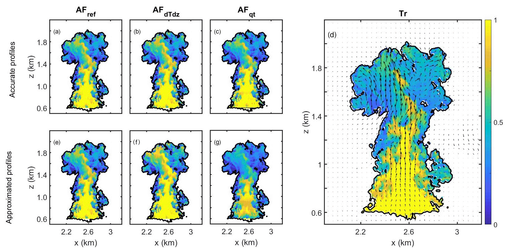
Figure 1 Cross sections of the tracer and the three AF methods presented for a cloud with a 500 cm⁻³ aerosol concentration at the time of its maximal top height. The AFs in the upper row were calculated using accurate adiabatic profiles of T and q_v. Profiles in the bottom row were approximated using high updrafts. (a) The method for calculating AF used as a reference (AF_ref) by solving Eq. (6). (b) Same as (a) for AF_dTdz using Eq. (8). (c) Same as (a) for AF_qt using Eq. (7). (d) Normalized concentration of the sub-cloud layer tracer (Tr). (e) Same as (a) for approximated profiles. (f) Same as (b) using approximated profiles. (g) Same as (c) using approximated profiles.

The vertical profiles of T and q_v that were used in Fig. 1a–c (based on the simulated Tr) can also be calculated using the maximal values of LWC or updraft. It is hard to obtain these types of profiles from in situ measurements that do not contain the theoretical tracer or the full 3D distribution of the cloud variables. Thus, for the sake of simplicity and in order for the methods presented in this paper to be comparable to measurements, we approximated the profiles by averaging the values in the voxels with the highest 5 % updraft values at each altitude. This methodology was used to estimate the T and q_v profiles throughout this study. It is shown that AF_ref remains almost similar when using either the approximated or accurate profiles. On the other hand, AF_qt and AF_dTdz exhibit some underestimation and overestimation compared to the accurate profiles, respectively. These differences are explained in detail below, and tests of sensitivity to the chosen profiles according to different thresholds on Tr values are presented in the Appendix for all three methods (Fig. A2). Figure 2 presents the differences between each AF method when using the approximated profiles and the Tr values (as shown in Fig. 1d). The apparently good agreement between AF_ref and Tr, as presented in Fig. 1e, is more closely examined in Fig. 2a, where differences are detected. In the first 100 m above cloud base the AFs experience non-realistic, non-homogenous values due to the inhomogeneity of the cloud base (in agreement with results of Romps and Kuang, 2010b). Moreover, the values of LWC and LWC_ad near the cloud base are small; hence, their ratio exhibits high sensitivity even when differences from the reference are minor (chosen according to the highest updraft). For the sake of comparison with Tr, the points near cloud base with AF > 1 were set to 1. Determination of the cloud-base height was achieved using the vertical profile of the cloud horizontal cross-sectional area. All clouds exhibited a local maximum in the cross-sectional area around 600 m during their growing stage. Aiming to choose the cloud base as a level that can represent the cloud with “enough” cloudy voxels, we chose to define it as the height above the level of initial condensation, in which the area covers 90 % of the local maximal area. Changing the criteria threshold from 90 % to 33 % can decrease the cloud-base height by up to 30 m. This definition, using the 90 % criteria, was found to be stable for all simulations during the growing stage of the clouds and is considered optimal for AF calculations since it maintains optimal agreement between AF_ref and Tr in the regions of high values. When comparing the cross sections of Tr with each AF presented in Fig. 1 (more than 100 m above cloud base), one can see that the AFs decrease toward the cloud edge faster than Tr (Tr > AF; see Fig. 2a). This is because AF is also affected by evaporation, and not only dilution, as in the case of Tr (i.e., mechanical mixing). The opposite is observed in higher levels in slightly diluted regions, where $\mathrm{Tr}<{\mathrm{AF}}_{\mathrm{ref}}<\mathrm{1}$. These regions represent a more complex difference between AF and Tr, which is also caused by condensation and/or evaporation. Tr can change only due to mechanical mixing and is hence almost a one-directional process; once the parcel is diluted, it has low probability to restore its initial Tr concentration. This means that Tr has a memory of the mixing history, unlike AF that can be influenced by source and sink processes. A parcel can regain liquid water after a mixing event if supersaturation is reached again at a later stage. Moreover, the parcel's condensation rate can be different from that predicted by the adiabatic parcel model because its droplet size distributions have changed and the local profiles of supersaturation can be very different from the ones of the core. This means that a parcel in the margins of the cloud can be diluted, decreasing both Tr and LWC (AF), but later, if the parcel gains vertical velocity and supersaturation, it might condense water at a rate that is larger than in the core. This will compensate for the LWC loss (keeping Tr the same, while increasing AF; i.e., $\frac{\mathrm{dLWC}}{\mathrm{d}z}>\frac{{\mathrm{dLWC}}_{\mathrm{ad}}}{\mathrm{d}z}$). The toroidal vortex seems to be a mechanism that drives such conditions. In Fig. 2a we show red regions of AF > Tr, which are voxels of relatively strong updrafts and are part of the flow pattern of the toroidal vortex (for an elaborated discussion about the vortex see Zhao and Austin, 2005). Using the velocity field, the regions of AF > Tr can be tracked back in time (back trajectory) to their earlier location, where the toroidal vortex entrains environmental air. Those parcels that mix with entrained air are first diluted and then flow upward driven by the flow in the toroidal vortex. These diluted parcels with low droplet concentration and high vertical velocity create high supersaturation values (higher than the values in the core for the same altitude). Hence, they condense water at a higher rate, which leads to a local increase in AF with altitude. The phenomenon of rapid growth of droplets in an updraft following an entrainment event was suggested as a mechanism for rain initiation (Baker et al., 1980; Yang et al., 2016). Correlations of the red regions (where AF > Tr) with strong updrafts (as part of the toroidal vortex), high supersaturation values, and low droplet concentration were found for different time steps and different cloud simulations.

Figure 2 Vertical cross sections for the differences between various AF methods, using approximated profiles (Fig. 1e–g), and the tracer (Fig. 1d). (a) Difference between AF_ref and Tr (Fig. 1e minus Fig. 1d). (b) Same as (a) for AF_dtdz. (c) Same as (a) for AF_qt.

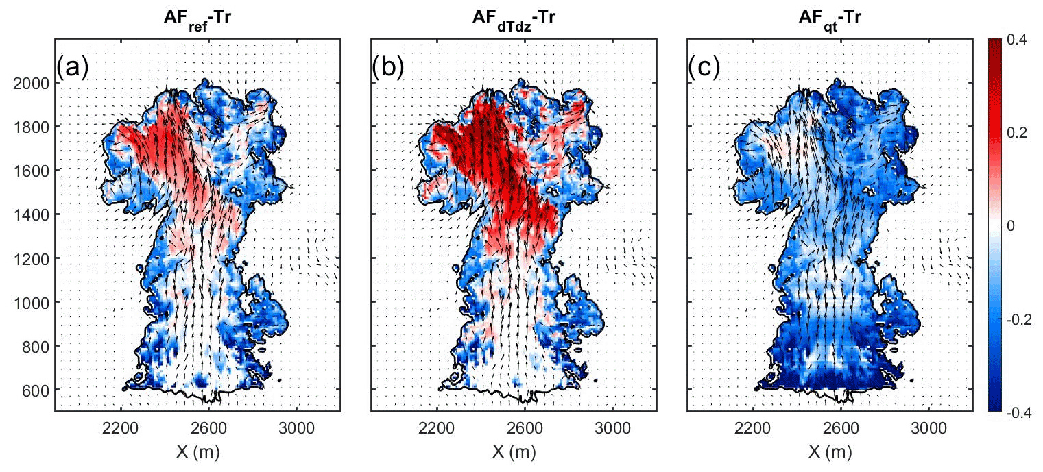
Figure 1f shows the cross section of AF_dTdz values, and Fig. 2b shows its difference from Tr. Here, very good agreement with AF_ref is observed, although AF_dTdz with the approximated profiles is slightly larger in the sub-adiabatic regions at higher levels (i.e., having smaller values of LWC_ad(z)). This is explained by the fact that AF_dTdz considers the difference between $\frac{\mathrm{d}T}{\mathrm{d}z}$ and the dry lapse rate as a consequence of condensation and uses it to define LWC_ad. Diluted parcels are colder than the adiabatic core because they were mixed with colder environmental air and may have experienced evaporation. This difference between absolutely adiabatic and slightly diluted parcels increases with height as the parcel is aging. For these reasons, using diluted voxels to estimate the adiabatic profiles will lead to a larger temperature gradient (more negative) that is closer to the dry lapse rate, falsely inferring less condensation and biasing LWC_ad toward smaller values. The arguments above explain the difference between Fig. 1a–b where AF_dTdz≈AF_ref and Fig. 1e–f where AF_dTdz > AF_ref. These findings suggest that AF_ref is less sensitive to the choice of adiabatic profiles because it is constrained by two free parameters (T and q_v) rather than only T. The final method, AF_qt, is shown to be very sensitive to the choice of profiles, as presented in Fig. 1c and g. The deviation from Tr in Fig. 2c demonstrates a substantial underestimation of AF_qt due to a similar argument as discussed above for AF_dTdz. Using a slightly diluted parcel, with a smaller q_v or q_vs compared to the core, is expected to falsely infer more condensation and larger LWC_ad. The bias is stronger for this method because it depends on q_v (or its estimation as q_vs(T)). The simplicity of this method is also its downfall; since q_v is an order of magnitude larger than q_l (liquid mixing ratio), small errors can cause significant effects when estimating LWC_ad using only q_v. Another disadvantage of AF_qt is that it is commonly used with the saturation adjustment assumption (i.e., S≈0) by estimating q_v to be q_vs. This assumption can lead to underestimation of AF_qt in conditions of a pristine environment (low aerosol concentrations) as explained in detail in Sect. 3.2.3. The results of this section suggest that the analytical solution for AF_ref using Eq. (5) is a more accurate and stable method to calculate AF, as it shows similarity to Tr and robustness for different choices of vertical profiles. We also note that profiles of T and q_v are often obtained from the environment (see Sect. 3.2.2). This will lead to substantial errors when using AF_dTdz or AF_qt, which showed sensitivity to the choice of profiles. Furthermore, Eq. (5) allows isolating different assumptions, such as linearity, with height and saturation adjustments.

3.2 Testing the effects of assumptions made when calculating AF

Next, we examine the effects of several commonly used assumptions on AF_ref calculation in order to estimate their impact. Although the magnitude of the difference that should be considered significant depends on the application, we define a considerable difference here as 0.1, which is 10 % of the maximal LWC_ad.

The approaches that will be examined next are the following:

1. AF_linear using Eq. (6) and keeping $\frac{A\mathrm{1}}{A\mathrm{2}}$ constant from the cloud base;

2. AF_env using the sounding (environmental) profiles in Eq. (6);

3. AF_s including the supersaturation term using Eq. (5);

4. AF₊₅₀ using Eq. (6) but estimating the cloud-base height to be 50 m higher; and

5. AF₋₅₀ using Eq. (6) but estimating the cloud-base height to be 50 m lower.

Each approach will be compared with the reference approach (AF_ref; Eq. 6). This method is not the most accurate one (method AF_s using Eq. 5 is), but since it is the base for all other examined assumptions, using it allows us to isolate and examine each of the assumptions separately.

Figure 3 Vertical cross sections of the differences between the various assumptions used when calculating AF. (a) The method of calculating AF that is used as the reference (AF_ref; as presented in Fig. 1e). (b) AF_ref subtracted from an AF that is linear from cloud base (AF_linear). (c) AF_ref subtracted from AF_env, calculated using sounding (environmental) profiles. (d) AF_ref subtracted from AF_s, which considers the supersaturation term (Eq. 5). (e) The error in AF caused by overestimating cloud base by +50 m. (f) Same as (e) with a −50 m error.

3.2.1 Linear LWC_ad

AF_linear is a very common method based on the assumption that LWC_ad is linear with height (i.e., neglecting the dependence of $\frac{A\mathrm{1}}{A\mathrm{2}}$ on temperature and humidity). This implies that $\frac{A\mathrm{1}}{A\mathrm{2}}$ can be used as a constant based on the known values at the cloud base (Pontikis, 1996; Yau and Rogers, 1996). Note that the derivation of AF using Yau and Rogers (1996) leads to the equation of $\frac{A\mathrm{1}}{A\mathrm{2}}$ at cloud base. Indeed, small negative differences from the nonlinear AF_ref (i.e., underestimation) are observed in Fig. 3b when using $\frac{A\mathrm{1}}{A\mathrm{2}}$ as a constant from the cloud base. Pontikis (1996) derived such a solution for stratocumulus clouds and noted that the error using this method would increase for deeper clouds. On the same note, Brenguier (1991) argued that the linear assumption is valid for shallow clouds (depth of up to 200 hPa, ≈2 km). This emphasizes that the usage of the AF_linear method is restricted to shallow clouds and should be used with care or avoided altogether for deeper clouds.

The changes in the growth rate of LWC_ad ($\frac{A\mathrm{1}}{A\mathrm{2}}$ in Eq. 6) with height, which can lead to deviation from AF_linear (or AF_env, discussed next), occur mostly due to changes in A₂. This is because A₁ (Eq. 2a), which is a parameter in the term for cooling by ascent, depends only on temperature and exhibits a negligible change in the case of our shallow clouds. A₂ (Eq. 2b), which relates to the S sink term (by condensation), depends on T and q_v and increases with height. Figure 4 demonstrates the sensitivity of A₂ to q_v and T by presenting the differences in the profiles of A₂ from the true profile (calculated using the original q_v and T profiles) and when keeping T or q_v as a constant (with the value set at cloud base). The true profile of A₂ (in blue) shows an increase with height, as mentioned earlier. One can see that the A₂ profile with a constant T (red curve) is very similar to the true profile. On the other hand, the profile's gradient decreases significantly when using q_v as a constant (yellow line). This demonstrates that depletion of water vapor in higher levels of the cloud is the major factor that impacts A₂ values (see the inverse relation to water vapor mixing ratio in Eq. 2b) and the deviation of LWC_ad from its linear relations.

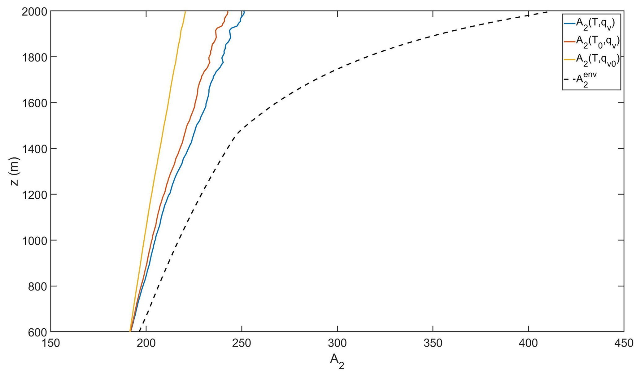
Figure 4 The sensitivity of the A₂ profile to temperature and humidity. The growth rate of LWC_ad depends on the ratio of $\frac{A\mathrm{1}}{A\mathrm{2}}$ (see Eq. 6). LWC_ad changes with height depend mostly on A₂, since A₁ exhibits little sensitivity. The blue curve is the true profile of A₂. Red and yellow A₂ profiles are calculated using constant temperature and humidity, respectively, and the dashed black line is the profile obtained using the environmental sounding.

3.2.2 LWC_ad using sounding profiles (environmental profiles)

The advantage of using environmental profiles is that they can be obtained from sounding data and can be considered constant reference values for an ensemble of clouds (the whole cloud field). Such an application can have large errors in cases in which the T and q_v profiles in the cloud's core and the environment exhibit large differences (e.g., penetration of the cloud into the inversion layer or into higher levels of the atmosphere). The profile of A₂ when calculated using the environmental profiles is given as a dashed black line in Fig. 4. It shows that the environmental A₂ profile values are larger than the profiles in the core of the cloud (especially in the inversion layer above 1500 m, where q_v decreases fast). The larger A₂ values lead to a smaller LWC_ad (A₂ is in the denominator in Eq. 6) and hence to an overestimation of LWC_env, as seen in Fig. 3c. The small overestimation witnessed in our case (trade wind cumulus in Barbados) will probably be greater for deeper clouds, wherein the gradients between the core and the environment are larger.

3.2.3 The role of the supersaturation term in conditions of low aerosol concentrations

Considering the profiles of T and q_v is necessary if one wishes to dismiss the saturation adjustment assumption (i.e., $\frac{\mathrm{d}S}{\mathrm{d}z}\approx \mathrm{0}$). This assumption is almost inherent in most previous works that we know of. The supersaturation can be significantly greater than zero in regions of high updrafts and/or small droplet concentrations (for example, in the first tens of meters above cloud base and in pristine environments). Thus, if one wants to achieve accuracy near cloud base or compare different clouds under different aerosol loading conditions (e.g., studying aerosol effects on cloud mixing), one has to use AF_s as calculated by Eq. (5). The second term in Eq. (5), referred to here as the S term, depends on the vertical profile of S. It is worth noting that S profiles are available only in modeling studies, since in situ measurements of S cannot reach the desired accuracy, as far as we know. Figure 3d demonstrates that for cases in which the cloud develops under conditions of high aerosol concentrations (N_a = 500 cm⁻³), neglecting the S term introduces a negligible underestimation of AF near the cloud base (AF_s>AF_ref). However, this is not the case for cleaner environments (lower N_a). Neglecting the S term means assuming that the parcel condenses all of the excess water vapor that forms as it ascends and cools. This overlooks the limited condensation efficiency in pristine environments that prevents a full consumption of water vapor by the drops and lets S increase (i.e., $\frac{\mathrm{d}S}{\mathrm{d}z}$ and the second term are larger than zero). To evaluate this effect, we simulated two additional clouds in a cleaner environment with lower aerosol concentrations (N_a = 50 and 5 cm⁻³). Before analyzing these simulations, we first had to make sure that there is no significant sedimentation in the clouds at this stage. Sedimentation creates liquid water loss and downdrafts, which violate the adiabatic assumption and lead to a deviation of AF from Tr. For the example examined in this section, we used Tr to ensure that sedimentation can be neglected in the time steps we chose for comparison (timing of maximal cloud-top height of each cloud). Figure A3 in the Appendix shows vertical cross sections of AF_ref and Tr for the cloud simulations with N_a = 50 and 5 cm⁻³ at the time steps used for this example. There is good agreement between AF_ref and Tr for N_a = 50 cm⁻³ at 33 min and N_a = 5 cm⁻³ at 31 min. This is not the case for N_a = 5 cm⁻³ after 40 min when the cloud precipitates and sedimentation can no longer be neglected. In Fig. A3 we observe regions in the clouds with large differences between Tr and AF_ref values.

In Fig. 5, we present the deviation of AF_s (when including the saturation term) from AF_ref for the three different simulations. Figure 5a (same as Fig. 3d) shows that the deviation is negligible for high N_a. The deviation increases and spreads to higher levels when N_a is smaller (Fig. 5b–c). Under pristine conditions (N_a = 5 cm⁻³, Fig. 5c), the underestimation of AF_ref spreads throughout the entire cloud column. The profiles of S are depicted in Fig. 5d for all cases, presented as the mean S of the voxels with the highest 5 % updraft in each level. Figure 5d shows that saturation adjustment is a reasonable approximation for AF calculations in polluted clouds because the S profile is smaller and, more importantly, almost constant. The gradient of the S profile of the N_a = 50 cm⁻³ case is also positive far from the cloud base (at 1000–1400 m). It does not introduce very large errors to AF_ref (as can be seen in Fig. 5b) because the gradient is relatively small, and thus the second term in Eq. (5) is negligible compared to the first term. Near cloud base, the first term in Eq. (5) is small, and thus even a relatively small gradient in S can be significant and lead to a large difference between AF_ref and AF_s.

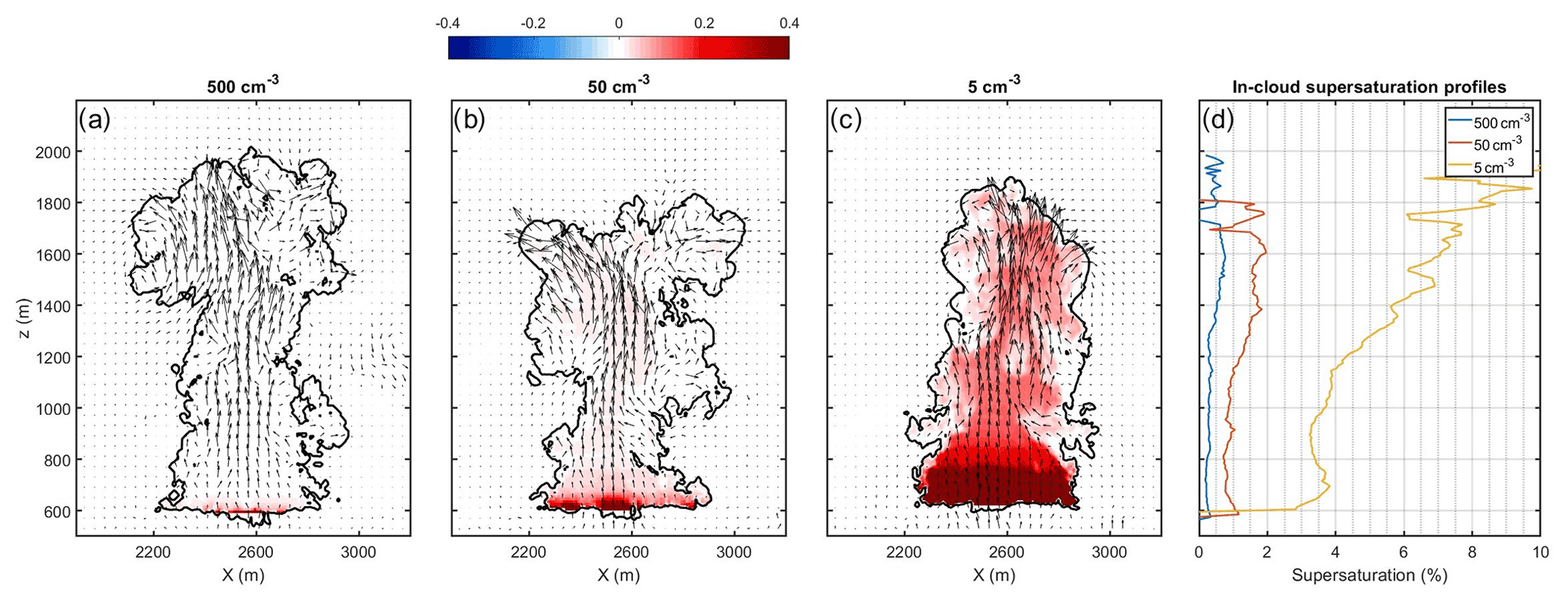
Figure 5 Microphysical effects on AF. The droplet concentration (i.e., aerosols) affects AF through the profile of supersaturation inside the cloud. Panels (a)–(c) present cross sections of AF_s (with the supersaturation term) minus AF_ref. (a) For high N_a of 500 cm⁻³ (as in Fig. 3d). (b) For 50 cm⁻³ at 33 min. (c) For 5 cm⁻³ at 31 min. (d) In-cloud supersaturation profiles.

3.2.4 AF sensitivity to cloud-base heights

Last, we tested how sensitive AF calculations are to the errors in the estimation of the cloud-base height. Figure 3e–f show the deviation from AF_ref when having an error of ±50 m in cloud-base height. When overestimating (underestimating) cloud-base height, as in Fig. 3e (Fig. 3f), the estimated LWC_ad is smaller (larger) and AF is larger (smaller). These results demonstrate that such small errors in a parameter that is often taken for granted can introduce large errors in adiabaticity estimation. For example, the lifting condensation level (LCL), which is often used to approximate cloud-base height, can be obtained from a tephigram or calculated by several proposed analytical equations. Calculating LCL from surface conditions, as suggested by Bolton (1980), Lawrence (2005), and Romps (2017), approximates cloud-base height to be 515, 550, or 525 m, respectively. These approximations are lower than the height that was found to be optimal for AF calculations using the sub-cloud layer tracer (≈600 m, depending on simulation time and cloud properties). Additionally, LCL is known to be an underestimation of cloud-base height when the convective parcel is driven by perturbation in temperature. In such a case, the perturbation reduces the parcel's relative humidity, and therefore the parcel starts the condensation at a higher altitude (above the LCL). This can cause an overestimation of LWC_ad and an underestimation of AF. The opposite will occur when the convection is driven by a humidity fluctuation (Hirsch et al., 2017). We note that most in situ measurements and spaceborne remote sensing observations lack the tools required to measure the cloud-base height and usually estimate it based on LCL.

3.3 Mean differences between the assumptions with time

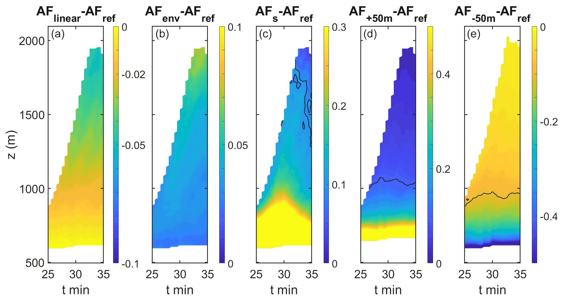
So far, we have examined the AF calculations at one time step of the time of maximum development of the clouds (∼33 min). The robustness of the results is tested by estimating the deviation of each method from AF_ref over height and as a function of time along the cloud's lifetime. Since the deviations are more pronounced in regions of high AF, for this analysis we chose to consider only the cloudy regions with AF_ref>0.5. Note that these sub-adiabatic regions are important and highly debated. Figure 6 shows the mean deviation for a cloud with N_a = 500 cm⁻³. Here, we observe that the statistics along the cloud's lifetime agree with the instantaneous qualitative pictures presented in Fig. 3. As demonstrated in Fig. 6a, the linear assumption (AF_linear) underestimates AF for altitudes above cloud base. AF_env, using the environmental profiles (Fig. 6b), exhibits a small overestimation, which becomes significant near the cloud top at the inversion layer. Here, we define a significant difference as larger than 0.1 in absolute value (marked by the black contour). Considering the S term in the polluted case does not have a considerable effect (Fig. 6c). Errors in the estimations of cloud base by 50 m lead to relatively large errors in AF- up to 1000 m (Fig. 6d–e). Repeating the same analysis for the clean case (with N_a = 5 cm⁻³) gives similar results for all methods but AF_s (see Fig. 7c), which supports the argument made in Sect. 3.2.3. The time series is shorter in this case because sedimentation starts after 33 min. It seems that the observed differences between the AF calculation methods do not change with time during the growth stage of a particular cloud for both pristine and polluted conditions.

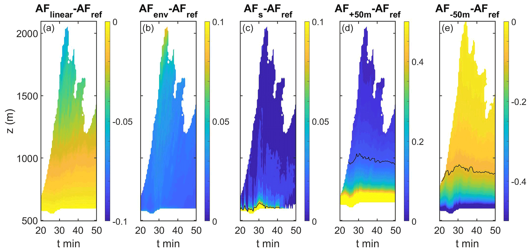
Figure 6 Mean differences in AFs vs. time and altitude for a polluted cloud. The horizontal average of the difference of each assumption from AF_ref for regions with AF_ref>0.5 is presented. (a) The difference between the linear method AF_linear and AF_ref. (b) Same as (a) for AF_env. (c) Same as (a) for AF_s. (d) The error in AF produced by an error of +50 m in cloud-base height. (e) Same as (d) for −50 m. The black contour marks the 0.1 or −0.1 deviation. Note the different scales for the different panels.

Figure 7 Mean differences in AFs vs. time and height for a clean cloud.

4 Summary and conclusions

An accurate calculation of the adiabatic fraction (AF) is crucial in two main aspects. First, it can promote a high-resolution measure of the mixing state of sampled parcels. This may advance the research of mixing processes in shallow clouds and their effects, which remain open questions in the field of cloud physics. Second, it can allow mapping the occurrence and extent of adiabatic regions in shallow clouds (which is still under debate). Since adiabatic processes are simpler to predict it is highly beneficial to assume them in remote sensing retrieval algorithms and cloud parameterizations in weather and climate models. Answering these questions can improve our process-level understanding, in situ measurements, and remote sensing retrievals. This will improve models' representation of shallow convection and may reduce the magnitude of the shallow clouds' contribution to the uncertainty in weather and climate models.

This study used high-resolution (10 m) simulations of isolated trade wind cumulus clouds that solved the turbulent flow down to scales that are rarely achieved. This enables a better representation of mixing and relaxes the dependency on sub-grid parameterization schemes. A sub-cloud layer's passive tracer (Tr), which is an accurate measure of mechanical mixing, was added to the simulations and used as a reference. This model configuration enabled better control of AF and the complex processes that it represents, as well as giving a theoretical framework that allowed testing the accuracy of different approaches that are commonly used to calculate adiabatic fraction (AF). Three different derivation methods of AF (Eqs. 5, 7, 8) were compared with the tracer. While the most robust method (Eq. 5) depends on both temperature and humidity profiles, the other two methods (Eq. 7, 8) depend on one variable (humidity or temperature, respectively). The method that is based only on humidity (Eq. 7) exhibited weaker agreement with Tr. Comparing AF with Tr also shows that some regions in the cloud emphasized the important differences between AF and Tr. While Tr follows the complex flow in the cloud and records all mixing events, AF is based on a one-dimensional model whose reference lies in the core. For that reason, AF cannot describe processes that occur in the margins. Moreover, condensation that occurs after a mixing event can delete records of earlier evaporation or dilution events. As an example, the toroidal vortex drives entrainment events followed by updrafts, which cause some parcels to experience dilution and evaporation (decrease in Tr and AF), followed by condensation that increases AF. The analytical structure of the reference method (Eq. 5) also allows us to isolate different assumptions and evaluate their accuracy. The important findings and their implications are as follows: assuming a linear profile of LWC_ad or using the sounding profiles of temperature and humidity instead of the in-cloud profile produces small errors at higher levels of shallow clouds (∼2 km). The small error in AF for shallow clouds obtained using environmental profiles suggests that it can be used as a constant reference for all clouds in the field.

The saturation adjustment assumption was integrated into the calculation of AF in most previous studies. Testing this assumption on clouds that develop in different environmental conditions (with different aerosol concentrations) revealed that it can lead to underestimation of AF. A simulation of a cloud in a pristine environment (N_a = 5 cm⁻³) yielded high supersaturation values (compared to the polluted case) and led to an underestimation of AF when assuming saturation adjustment (i.e., $\frac{\mathrm{d}S}{\mathrm{d}z}\approx \mathrm{0}$). This means that comparing clouds' mixing under different aerosol loading when using the saturation adjustment assumption may neglect some of the microphysical effects on clouds' dynamics, mixing in particular.

AF was found to be sensitive to errors of ±50 m in the estimated cloud-base height, especially in the first few hundred meters above cloud base. Determining cloud-base height is challenging for aircraft in situ measurements and is often obtained by estimating the lifting condensation level (LCL) from a tephigram or analytical solutions. The three analytical solutions that were tested here (Bolton, 1980; Lawrence, 2005; Romps, 2017) differed by 45 m and underestimated the cloud-base height that was optimal for AF calculations. Underestimation of the cloud-base height can lead to a larger LWC_ad and thus to the underestimation of AF. This can lead to an underestimation of the extent of adiabatic regions in shallow clouds. Accurate estimation of AF near the cloud base is challenging because these levels include a ratio of two small numbers (LWC and LWC_ad) and are not homogenous as mostly assumed. Moreover, the calculation of LWC_ad in these levels exhibits high sensitivity to the determination of cloud base and the representative supersaturation profile.

All simulations demonstrated the existence of an adiabatic core (i.e., high values that are close to 1 for both AF and Tr) up until the cloud top. While the core is wide at the lower parts of the cloud, it narrows and breaks down to smaller fragments at higher levels. The extent and frequency of adiabatic parcels in different levels of the cloud will be assessed in a subsequent study.

And in short, here are the main points to consider when practically calculating AF.

• 1.

  Calculations of AF will be most robust when using Eq. (5) (or Eq. 6 in polluted conditions), including the linear assumption when it is valid (Yau and Rogers, 1996).

• 2.

  When using AF for studies of aerosol–cloud interactions by comparing different parameters conditioned by AF, one cannot make the saturation adjustment assumption as it underestimates AF in pristine conditions and can bias the results.

• 3.

  AF is most sensitive to the definition of cloud-base height. Thus, it is important to make sure that the chosen value represents the investigated cloud or clouds well at the altitude in which most parcels start to condense water.

• 4.

  AF in deep convective clouds is prone to many large errors, and the uncertainty of the calculations is hard to assess, mainly in relation to the following.

  • a.

    AF is based on a quasi-hydrostatic equation, which is valid for updrafts smaller than 10 m s⁻¹.

  • b.

    Supersaturation in clouds with strong updrafts can increase, leading to underestimations of AF when the S term is neglected.

  • c.

    Sedimentation of particles from higher levels of deep clouds can increase LWC in the lower levels and lead to an overestimation of AF.

  • d.

    The rate of change in LWC_ad is dominated by the parameter A₂, which changes as water vapor is depleted in clouds, meaning that LWC_ad ceases to be linear. The large differences expected in deep clouds between the in-cloud and environmental profiles suggest that the latter are prone to large biases when used to predict AF.

Appendix A

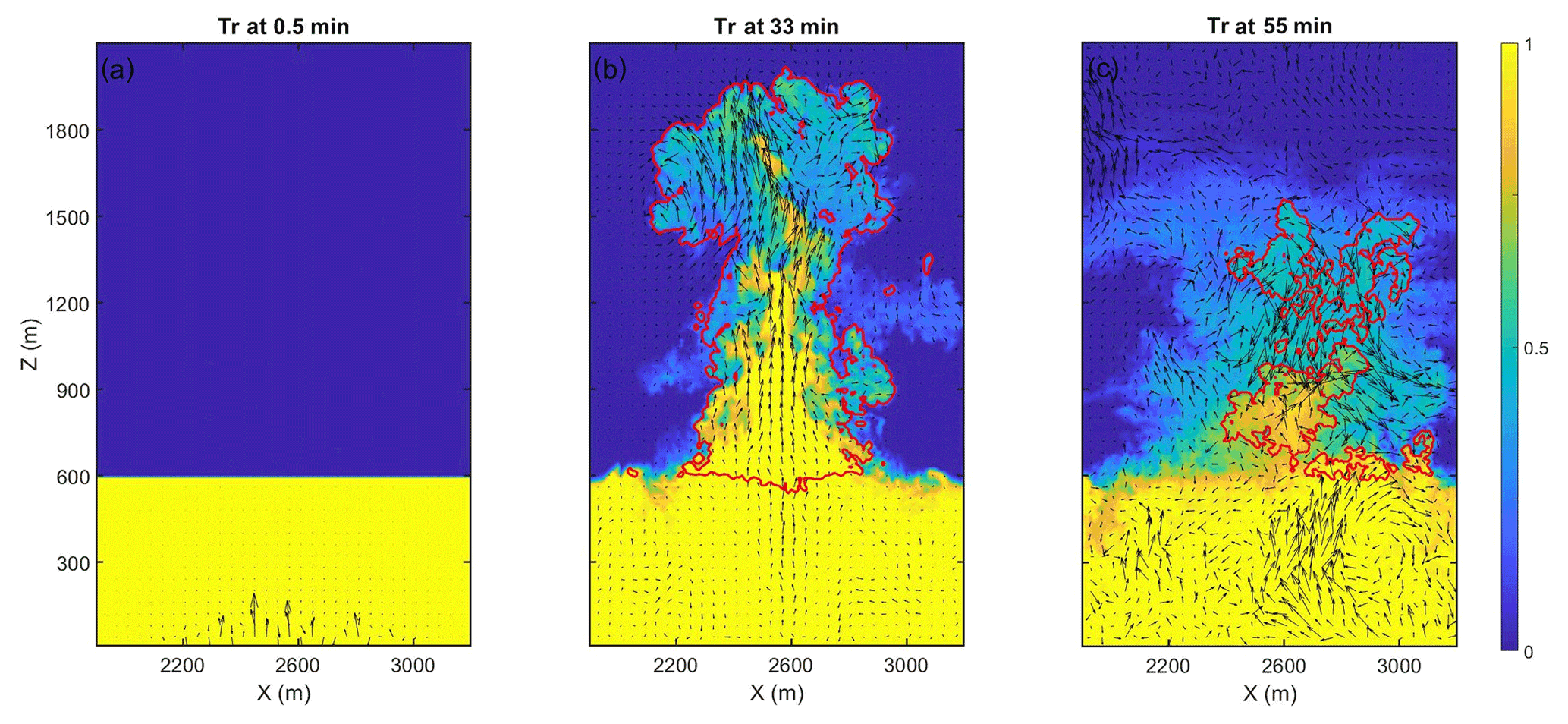
Figure A1 The sub-cloud layer's passive tracer. Vertical cross sections of the tracer along the x axis in the middle of the domain. Tr is the tracer's mixing ratio normalized by its initial mixing ratio in the sub-cloud layer. (a) The initial distribution at the beginning of the simulation. (b) Distribution at the time of the cloud's maximal development (33 min). Red contours mark the cloud boundaries where the liquid mixing ratio is smaller than 0.01 g kg⁻¹. (c) Same as (b) for the end of the simulation when the cloud is nearly completely dissipated.

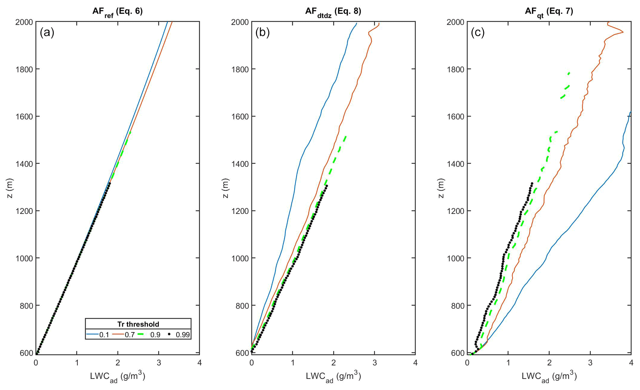
Figure A2 LWC_ad profiles of different approaches for different estimations of adiabatic profiles. LWC_ad(z) was calculated according to Eqs. (6, a), (8, b), and (7, c). Taken from a snapshot of a cloud with an aerosol concentration of 500 cm⁻³ at the time of maximal development (33 min). The temperature and humidity profiles were used by averaging all points of each layer according to a certain threshold on sub-layer tracer normalized concentration (Tr). Black dots are for nearly pure undiluted parcels with Tr > 0.99, the green dashed line is for nearly adiabatic parcels (Tr > 0.9), and red and blue curves also include slightly (Tr > 0.7) and strongly diluted (Tr > 0.1) parcels. It is shown that there are no pure adiabatic parcels above the inversion. Nevertheless, the use of slightly diluted parcels (with Tr > 0.7) in our chosen reference method (Eq. 6) does not introduce large biases to LWC_ad and AF accordingly.

Figure A3 Comparison of AF_ref and Tr for low N_a. Cross sections of AF_ref and Tr for lower N_a simulations. (a) Tr for 50 cm⁻³ at 33 min. (b) Same as (a) for AF_ref. (c) Tr for 5 cm⁻³ at 31 min prior to intense sedimentation. (b) Same as (c) for AF_ref. (e) Tr for 5 cm⁻³ at 40 min during intense sedimentation. (f) Same as (e) for AF_ref.