the Creative Commons Attribution 4.0 License.
the Creative Commons Attribution 4.0 License.
 | 21 Oct 2021
Estimation of the terms acting on local 1 h surface temperature variations in Paris region: the specific contribution of clouds
Oscar Javier Rojas Muñoz
Marjolaine Chiriaco
Sophie Bastin
Justine Ringard
Local short-term temperature variations at the surface are mainly dominated by small-scale processes coupled through the surface energy balance terms, which are well known but whose specific contribution and importance on the hourly scale still need to be further analyzed. A method to determine each of these terms based almost exclusively on observations is presented in this paper, with the main objective being to estimate their importance in hourly near-surface temperature variations at the SIRTA observatory, near Paris. Almost all terms are estimated from the multi-year dataset SIRTA-ReOBS, following a few parametrizations. The four main terms acting on temperature variations are radiative forcing (separated into clear-sky and cloudy-sky radiation), atmospheric heat exchange, ground heat exchange, and advection. Compared to direct measurements of hourly temperature variations, it is shown that the sum of the four terms gives a good estimate of the hourly temperature variations, allowing a better assessment of the contribution of each term to the variation, with an accurate diurnal and annual cycle representation, especially for the radiative terms. A random forest analysis shows that whatever the season, clouds are the main modulator of the clear-sky radiation for 1 h temperature variations during the day and mainly drive these 1 h temperature variations during the night. Then, the specific role of clouds is analyzed exclusively in cloudy conditions considering the behavior of some classical meteorological variables along with lidar profiles. Cloud radiative effect in shortwave and longwave and lidar profiles show a consistent seasonality during the daytime, with a dominance of mid- and high-level clouds detected at the SIRTA observatory, which also affects near-surface temperatures and upward sensible heat flux. During the nighttime, despite cloudy conditions and having a strong cloud longwave radiative effect, temperatures are the lowest and are therefore mostly controlled by larger-scale processes at this time.
- Article
(8508 KB) - Full-text XML
- BibTeX
- EndNote


Regional climate variability is to the first order driven by large-scale atmospheric conditions. In western Europe, the North Atlantic Oscillation (NAO; Trigo et al., 2002), which is associated with the locations and intensities of the centers of the Iceland low and the Azores high, controls the air mass advection over western Europe and explains a large part of weather variability. Temperature and pressure conditions are then modulated by the complex terrain (Mediterranean sea, topography, surface heterogeneities): extreme events and temperature anomalies are generally not exclusively explained by the presence of these large-scale air mass circulations (Vautard and Yiou, 2009). Indeed, synoptic and mesoscale atmospheric processes have been previously studied to explain interannual temperature changes in some parts of Europe (Efthymiadis et al., 2011; Xoplaki et al., 2003), or even precipitation occurrence (Xoplaki et al., 2004; Bartolini et al., 2009). It is, therefore, necessary to consider small-scale processes such as surface–atmosphere interactions and cloud feedbacks to better explain near-surface temperature variations (e.g., Chiriaco et al., 2014).
Temperature variations at the surface are related to the surface energy balance (SEB) following surface–atmosphere interactions and solar radiation (Wang and Dickinson, 2013) that are separated into different components: latent and sensible heat fluxes (Flat and Fsens, respectively), ground heat flux, temperature advection, and atmosphere radiation. Studies have been made to parametrize these terms when direct measurements are not available (Miller et al., 2017; Arnold et al., 1996), but their exact contribution is uncertain. Depending on the timescale considered, the importance of each SEB term for temperature variations will change (Bastin et al., 2018; Ionita et al., 2015).
The first objective of the current paper is to quantify the specific local contribution of the primary SEB terms acting on short-term (i.e., hourly) temperature variations in a western European location and to determine their importance and the conditions when a certain term predominates over the others, based on a simple linear model. The current study is inspired by Bennartz et al. (2013), who implemented a temperature variation model to study the influence of low-level liquid clouds over the Arctic on the ice surface melt period in July 2012, by estimating all of these SEB terms for a case study. Here, the same approach is used for a different location (mid-latitude) and on a long time period to get robust statistics. To do so, the study is based on direct measurements from the SIRTA-ReOBS dataset (Chiriaco et al., 2018), which includes many variables collected since 2002 at SIRTA (Site Instrumental de Recherche en Télédetection Active; Haeffelin et al. 2005), an observatory located in a semi-urban area in the southwest of Paris, France. This dataset is well suited to the current study objective because (i) it allows the use of a multi-variable synergistic compilation to study and compare different characteristics of the atmosphere or the surface (e.g., Bastin et al., 2018; Dione et al., 2017; Cheruy et al., 2013; Chiriaco et al., 2014), and (ii) it is located in western Europe and allows access to the hourly timescale, i.e., the scales of the local processes of the current study. The SIRTA-ReOBS dataset, along with some variables retrieved from ERA5, enables the development of a model to estimate all the terms involved in the near-surface temperature variations using predominantly real observations. The use of the model developed in the current study considers all the variables acting within the atmospheric boundary layer (ABL) and controlling surface temperature variations, all of them estimated almost exclusively from surface-based observations. Thus, it allows us to separately study the influence of each SEB term in a local scale. This indeed allows a realistic and reliable estimation of the contribution of each term (radiative fluxes, turbulent heat fluxes, etc.) on hourly temperature variations, and it would be possible to have that at different sites since each term will present a different behavior and importance. These estimations could help improve the parametrizations of the SEB terms that already exist and better understand their spatial evolution as a function of local conditions. Furthermore, a comparison between multi-model regional climate simulations and these estimations can be performed to evaluate whether the simulations are able to well reproduce these behaviors, in particular in a warming climate where these processes are expected to change. The weight of each term of the SEB on hourly temperature variations is analyzed using a powerful random forest analysis, one of whose attributes is its capacity to handle up to thousands of input variables and identify the most significant ones.
Clouds are well known to directly modify near-surface temperatures and other near-surface variables on multiple timescales (Parding et al., 2014; Broeke et al., 2006; Kauppinen et al., 2014). Hence the second objective of the current study is to understand the specific role of clouds and their associated characteristics in hourly temperature variations. Indeed, the influence of clouds on the temperature at the surface can vary depending on their physical properties and the altitude where they are formed (Hartmann et al., 1992; Chen et al., 2000). In general, low-level clouds tend to cool the surface, whereas high-level clouds, such as cirrus clouds, tend to warm it by absorbing a significant amount of Earth's outgoing radiation. The average contribution of clouds is to decrease the near-surface temperature, combined with the damping effects of soil moisture, from a global point of view, by reflecting the solar radiation to space. But their damping effects vary depending on the season and by time of day. For instance, the reduction in near-surface temperature is the highest in fall in the northern mid-latitudes for specific cases when precipitation is not significant (Dai et al., 1999). The local contribution of clouds to temperature variations is thus an important topic to assess how this intake affects local climate variability and extreme local events, such as the extreme heatwave and drought during summer in the EU in 2006 (Chiriaco et al., 2014; Rebetez et al., 2009) or the sudden melt of the ice sheet in Greenland on July 2012 (Bennartz et al., 2013). Several studies were made primarily focusing on the large-scale effects of clouds on the radiative energy balance on a global scale, either at the top of the atmosphere (Arkin and Meisner, 1987; Raschke et al., 2005; Dewitte and Clerbaux, 2017; Willson et al., 1981; Allan et al., 2014; Cherviakov, 2016) or at the surface (Wild et al., 2015; Hakuba et al., 2013; Wild, 2017) or both at the same time (Hartmann, 1993; Kato et al., 2012; Li and Leighton, 1993), but a lack of studies investigating their impact on a smaller scale is noted due to limited reliable ground-based measurement availability. In this study, to understand how clouds influence the 1 h temperature variations, cases with a particular cloud effect on temperature variations are more deeply analyzed using lidar profiles.
To achieve these two objectives, the current paper is organized as follows: the dataset is presented in Sect. 2. Section 3 (and Appendix A) describes how the different terms acting on hourly temperature variations are estimated and evaluates how well the model fits the hourly observations based on statistics. Section 4 presents an assessment to determine which term dominates at different times by performing a random forest analysis firstly for day and night cases and then separated in a diurnal cycle perspective, along with a mean monthly–hourly and annual cycle analysis of the contribution of each term. Section 5 focuses on a discussion to study the specific role of clouds and the atmospheric conditions under which they develop by assessing only the cloudy cases, which gives an overview of the type of clouds and surface conditions damping or enhancing near-surface temperature for both daytime and nighttime. Section 6 draws conclusions and provides perspectives opened by this work.
2.1 Data used for the temperature variation estimation model
This study is mainly based on the SIRTA-ReOBS dataset analysis. The SIRTA observatory (Haeffelin et al., 2005) is located in a semi-urban area 20 km southwest of Paris (48.71∘ N, 2.2∘ E) and has collected long-term meteorological variables since 2002. The ReOBS project aims to synthesize all observations available at a single observatory at an hourly timescale with exhaustive data-quality control, calibration, and rigorous treatment into a single NetCDF file. The SIRTA-ReOBS dataset (Chiriaco et al., 2018, https://doi.org/10.5194/essd-10-919-2018) contains more than 60 variables.
All the necessary hourly variables requested by the current study are available for the period from January 2009 to February 2014 and are listed in Table 1, allowing a multi-year analysis. Some variables that were retrieved from measurements at the SIRTA observatory sometimes present gaps due to instrumental issues (Chiriaco et al., 2018; Pal and Haeffelin, 2015). In particular Flat and Fsens variables are limited (with only 5 % and 73 % availability, respectively): Sect. 3 and Appendix A show how this issue is handled.
Table 1Variables available in the SIRTA-ReOBS dataset used as inputs in the temperature variation model. * TMLD is also estimated using the ERA5 dataset.

Figure 1 shows the complete dataset availability in the SIRTA-ReOBS dataset for the 5-year study period. The availability of data is quasi-homogeneous around 60 % for all hours (Fig. 1a). Most of the time gaps are due to the absence of the mixing layer depth (MLD) variable for some complete days, extended sometimes for more than 2 months (not shown), restricting 71 % of MLD data availability. Other gaps are caused by the absence of radiative variables (9 % of missing data; see Table 1). Summer is the season with the best data coverage (70 %), and winter has the least data coverage (56 % – Fig. 1b), whose absences are due precisely to gaps in the MLD variable.
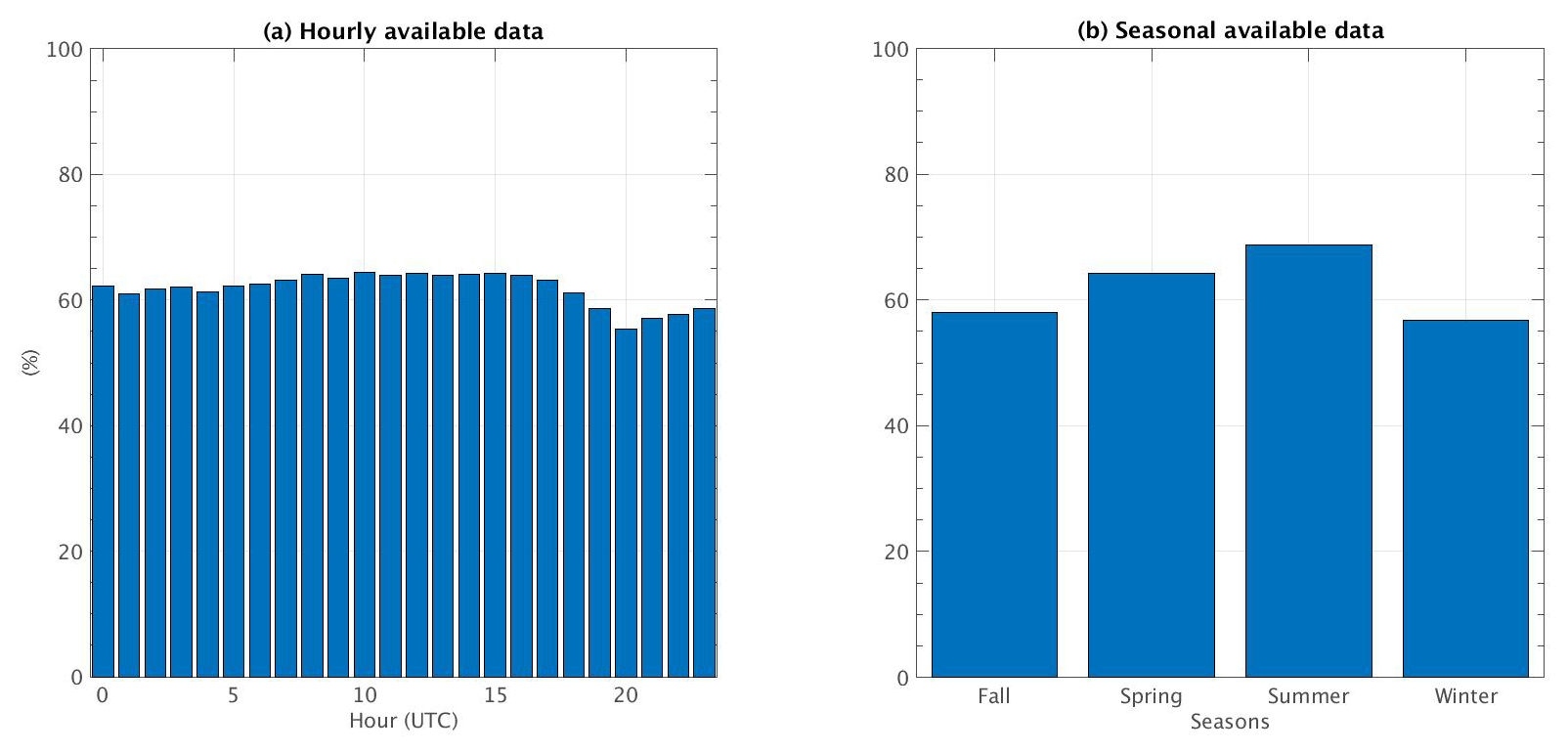
Figure 1Histograms of (a) hourly and (b) seasonal available data in the SIRTA-ReOBS dataset, considering all the variables needed for the period of study 2009–2014 for the temperature variation model.
To complete this dataset, hourly ERA5-Land (horizontal resolution of 0.1∘ × 0.1∘; Copernicus Climate Change Service, 2019) is used to estimate the horizontal wind at 10 m and the temperature near the surface T2 m, as required for the advection term (see Sect. 3 and Appendix A). Furthermore, the temperature at the mixing layer depth (TMLD) is also retrieved from the ERA5 (spatial resolution of 31 km and 137 levels up to 1 hPa; ERA5, 2020).
2.2 Variables used for the cloud contribution analysis
In order to get vertical information about clouds (see Sect. 5), SIRTA-ReOBS lidar profiles are also used, retrieved from a LNA lidar (532 and 1064 nm) whose vertical resolution is 15 m (for further details, see Chiriaco et al., 2018), and their analysis is based on hourly lidar scattering ratio (SR) altitude–intensity histograms, calculated as follows:
where ATB(z) is defined as the total attenuated backscatter lidar signal, and ATB(z)mol is the signal in clear-sky conditions. These altitude–intensity histograms are used to estimate the mean cloud fraction percentage at a given altitude level z. The intensity axis which contains SR(z) thresholds as well as the three vertical atmospheric layers (i.e., low, middle, and high layers) for cloud detection and characterization are defined in Chepfer et al. (2010). The value of corresponds to non-normalized profiles, the value −777 represents the profiles that cannot be normalized due to the presence of a very low opaque cloud, and the value of −666 is set as invalid data. Then, bins located in the range are for clear-sky conditions and is defined as unclassified data. For cloud detection, a threshold of SR(z)>5 is set. Details are given in Chiriaco et al. (2018). Even though the instrument does not operate uninterrupted (it does not operate when it is raining, when it is nighttime, and on the weekends), it is very powerful to get information on the vertical structure of the atmosphere.
The exchange of energy between the surface and the overlying atmosphere involves four terms: radiation, heat exchange with ground, heat exchange with the free atmosphere, and advection. In this section, a model which estimates these four terms is presented, based on several meteorological observations retrieved from the SIRTA-ReOBS dataset. Each term involved in this model is described (further descriptions are presented in Appendix), and then a statistical evaluation is performed to assess how well the model follows the real observations of temperature variations. Finally, the mean monthly–hourly and annual cycles of the averaged contribution of each term and the same for 1 h temperature variations () are presented (split into day and night).
3.1 Model description
The temperature variation at the surface is estimated from the sum of four terms:
where R is the net radiative flux at the surface, HG is the ground heat exchange, HA is the atmospheric heat exchange, and Adv is the air advection. These four terms control the changes in temperature over the surface, but depending on the temporal scale, one will dominate over the others (Ionita et al., 2012). Following Appendix A and partly based on Bennartz et al. (2013), these four terms are expressed as
Then
where T2 m is the near-surface temperature, t is the time (in hours), α is a coefficient characterizing the form of the temperature vertical profile in the boundary layer, ρ is the average air density of the boundary layer, cp is the specific heat of air, MLD is the mixing layer depth, ΔFNET is the net radiative flux at the surface, Ts is the temperature in the ground at 20 cm depth, TMLD is the temperature at the top of the boundary layer (or mixed layer depth), u10 and v10 are the zonal and meridional wind components, respectively, at 10 m above the ground, x is the zonal wind component towards the east and y is the meridional component wind towards the north, and τs and τa are defined as relaxation timescales for heat exchange processes in the ground and the atmosphere, respectively.
If the model is realistic, then the sum of the four terms on the left side of Eq. (2), denoted as , is as close as possible to the observed temperature variations denoted as .
The net radiative flux at the surface is calculated as the difference between the radiative longwave (LW) and shortwave (SW) fluxes leaving and arriving at the surface as follows:
where the upward and downward arrows represent the upwelling and downwelling radiation, respectively. It is possible to add and subtract the clear-sky (CS) downwelling radiation fluxes to Eq. (8), to obtain the flux radiative components in CS and cloudy (CL) conditions (i.e., the specific contribution of clouds), as follows.
Here, the flux is the same for clear-sky and cloudy conditions, because it mostly depends on the near-surface temperature (i.e., the Stefan–Boltzmann law, , where σ is the Stefan–Boltzmann constant), but note that in an annual global mean, (around 0.5 W m−2; Allan, 2011) due to the increase in longwave radiation emitted toward the surface by clouds, where a small proportion of this radiation is reflected by the surface.
Hence Eq. (2) becomes
with and ΔFNET,CS.
This formulation specifically allows estimation of the role of clouds (RCL) in temperature variations, compared to the other terms. Details on how each term is estimated along with the assumptions that have been made are stated in the Appendix.
As shown by Eqs. (3) to (6) and in Eqs. (A10) to (A17) in Appendix A, temperature variations are estimated from variables described in Sect. 2, i.e., predominantly based on observations retrieved from SIRTA-ReOBS, but also on ERA5 datasets.
Concerning the advection term, the computation of this term requires the extraction of the temperature at 2 m (T2 m) and northward (v10 m) and eastward (u10 m) wind components at 10 m, at the SIRTA grid point and the surrounding grid points. The temperature at the mixing layer depth TMLD is retrieved using SIRTA-ReOBS combined with ERA5 datasets. First, radiosoundings available in SIRTA-ReOBS (twice a day) are used to get the pressure at the MLD level, and then TMLD is retrieved from the vertical temperature profile in ERA5 at the nearest grid box from SIRTA Observatory (48.7∘ N and 2.2∘ E) and at this pressure level but at the closest time. Note that uncertainty remains in TMLD because it is the temperature at a certain pressure level, which is only available twice a day.
3.2 Statistical evaluation of the model
Statistics are considered to assess how close the total model () is to the observed temperature variations (). The PDFs of each term in Eq. (2) are shown in Fig. 2a. Firstly, the radiative term R dominates, and contributes the most in the temperature variations at an hourly scale since its distribution presents different significant peaks for negative and positive values of temperature variations. In clear-sky conditions, the radiative term contributes the most to warm the surface, whereas the radiative effect of clouds has an opposite effect. A significant negative contribution by the HA term is also observed (light brown line), meaning that the mixing with an atmosphere of higher levels contributes to decrease surface temperature variations, even if surface temperatures continue increasing along the day. The two other terms (HG and Adv) have a similar but weak impact on the temperature variation model at this timescale. In addition, the PDF of the is compared to in 1 h in Fig. 2b: differences occur for cases where the temperature decreases during the hour, but these differences correspond to some cases where the model presents more negative values than the observations, around −1 ∘C h−1. The modeled PDF fits very well with the observed PDF for cases where temperature increases during the hour (a smaller number of cases as shown by the PDFs).

Figure 2PDFs of (a) radiation (red line), radiative clear sky (red dashed line), radiative cloud (red dotted line), ground heat (dark brown line) and atmospheric heat (light brown line) exchange, and advection (cyan line) terms. (b) (pink line) and the (blue line). (c) Scatter plot of vs. . The sloping solid line represents the 1 : 1 line, and the dashed line corresponds to the least-square best fit linear regression line between the two datasets. The correlation coefficient r and the linear equation fitting the best for the two datasets are also indicated. (d) Hourly evolution for September 2010 of the temperature variation for the different terms, the observations, and the model (same colors as in a and b).
Figure 2c shows the scatter plot of the observations versus the model. The correlation between the two datasets is good (0.79) and the bias remains small (−0.20 ∘C h−1). However, the model has difficulties in reproducing the extremes of temperature change within an hour, e.g., −6 ∘C h−1, which corresponds to the 5 July 2011 at 20:00 UTC, or −8 ∘ C h−1, which corresponds to the 2 July 2010 at 15:00 UTC. This high decrease in temperature could be associated with a cold pool event, which is more detectable in summer thanks to higher near-surface temperatures than those in winter and bring along with it storms and heavy precipitations, as detected for these two cases (not shown). The hourly values in the observations (as well as in ERA5) do not allow the capture of this cold pool event properly in the model developed, since it is related to rapid cloud formation (<1 h) that is not well captured by the RCL term. However since this type of event is rare and ephemeral on a local scale (Llasat and Puigcerver, 1990; Conangla et al., 2018), its presence does not significantly bias the general performance of the model.
These statistics are estimated for each season as presented in Table 2. Correlation is high (0.82) and bias is low in summer. Nevertheless, the standard deviation remains high for this season, probably due to the higher values of temperature variation and the contribution of all terms involved for the summer in comparison to other seasons. For the spring and fall seasons, the correlation coefficient is still high (0.80). However, in winter the correlation coefficient is the lowest (0.67) with a higher bias (−0.31 ∘C h−1). Removing the extreme values of the observations and the model (i.e., taking the values that are within the 5th and 95th percentiles) gives better statistics (values in brackets in Table 2), confirming that the model encounters difficulties in reproducing these extreme events.
Table 2Statistics values between and for the four seasons of the year. The values in brackets correspond to the statistics within the 5th and 95th percentiles.
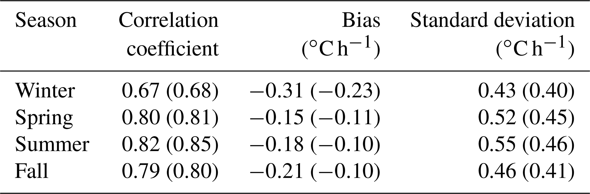
Figure 2d presents the hourly evolution of the five terms on the right side of Eq. (10), their sum (i.e., as blue solid line), and (pink solid line) for the first days of September 2010. As expected, a diurnal cycle is identified for the radiative (both cloud and clear-sky terms) and heat atmosphere exchange terms. For the radiative terms, it is quite expected to have a positive (negative) contribution during daytime (nighttime) due to the presence (absence) of solar radiation. In addition, there are some days when RCL (dotted red lines) plays an important modulating role in temperature variations, noticed during the day on 6 and 8 September, when clouds manage to provide a maximum cooling effect of −2.9 ∘C h−1.
Evaporation and thermal conduction at the surface increase as the day goes on, and the larger these terms are the more they will prevent the increase in temperature linked to the sensible and latent turbulent fluxes. But overall the temperature increases during the day when these fluxes increase. However, the atmospheric heat exchange term (HA) is on average a negative contribution to temperature variations in 1 h when Flat and Fsens increase in the afternoons. This negative contribution could be mostly associated with the mixing of masses of air at the top of MLD, where depending on the state of temperature inversion, TMLD is likely to be very negative and this cold air could cool the surface. When RCL presents an important contribution, HA becomes weaker and its diurnal cycle is attenuated due to the absence of solar radiation, and hence fewer surface fluxes are developed. The ground heat exchange and the advection terms play a minor role at this timescale and contribute negligibly to the model without a significant diurnal cycle detected.
Finally, the model follows the observations well, with a better agreement for daytime than for nighttime and with a better correlation for the first case (not shown). Reasons that may explain the bias are (1) the limited availability of TMLD data, which are estimated using only two radiosoundings per day and not continuous hourly values, and (2) the hypothesis and assumptions in some variables and atmospheric conditions outlined in Eqs. (A3) and (A4). Further, the temperature variations at night might be hard to quantify accurately due to the minor contribution of each of the non-radiative terms, for which contributions are close to zero, especially for the HA term, and where Flat and Fsens are very low most of the time (Sect. 3.3).
3.3 Annual and monthly–hourly cycles of the different terms
The mean contributions of each term are averaged monthly for both day and night (Fig. 3), whereas Fig. 4 presents the magnitudes of the monthly–hourly mean values from January 2009 to February 2014 of each term of the model. A residual term is calculated on these figures, which is calculated as the difference between the model (sum of all terms) and the observations (i.e., ).
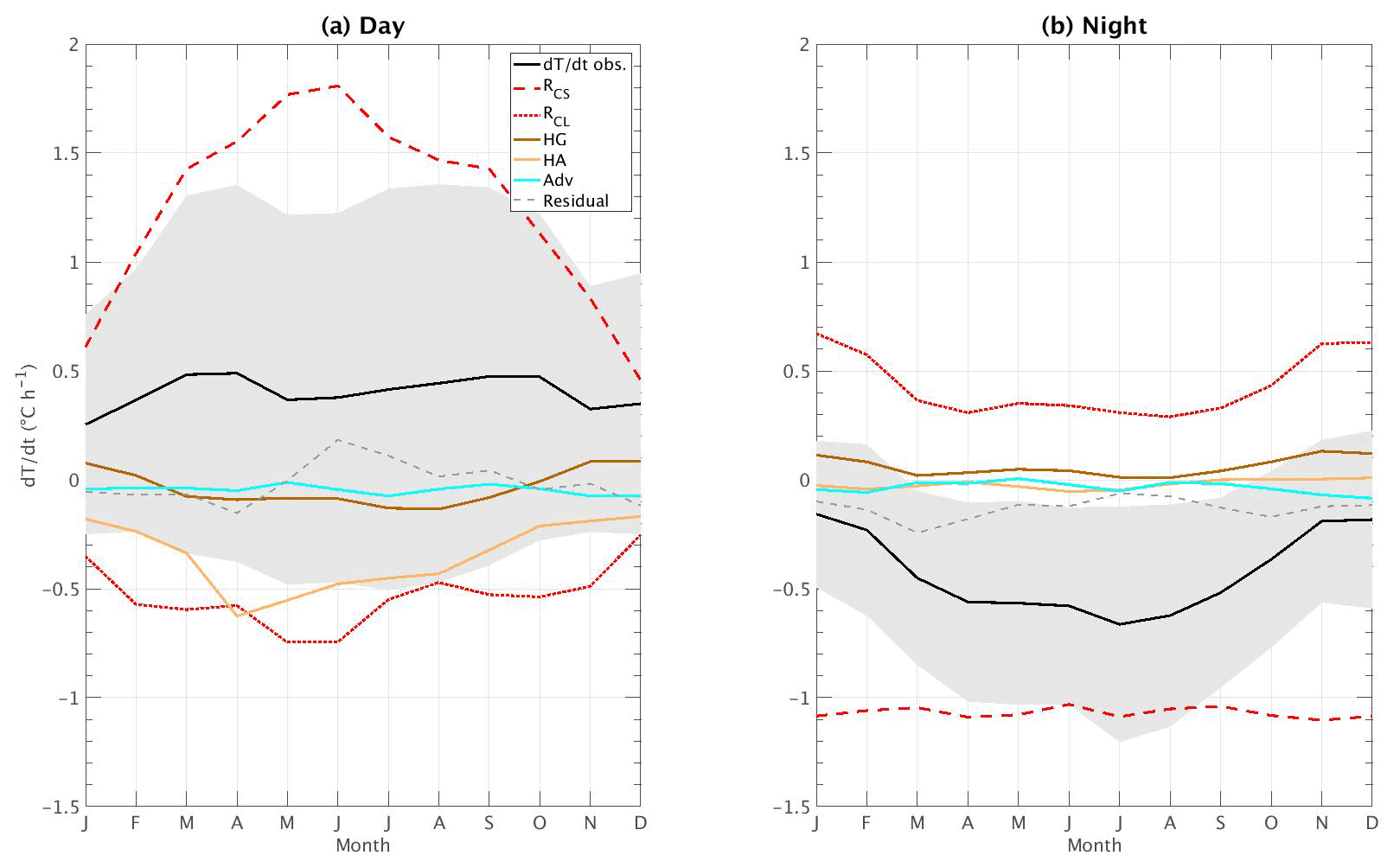
Figure 3Mean annual cycle averaged monthly from 2009 to 2014 of the five terms of the model, the observations, and the residual (dashed gray lines) for (a) day and (b) night. Same colors as in Fig. 2a and b. The shaded gray area in each of the panels represents the standard deviation of .
According to Figs. 3b and 4b for nighttime, the clear-sky and cloud radiative forcing terms dominate the hourly temperature variations in magnitude at the surface, and the other terms remain close to zero. Still, during the night, monthly mean is negative throughout the entire year, with higher negative values during warm months than during winter. Indeed, RCL is always positive during the night and has an annual cycle more pronounced than the other terms, having a stronger effect in the cold months, due to the increase in cloud cover, especially low-level clouds, which enhance an increase in the downwards flux of LW radiation and whose effect gets weaker while approaching summer, due to the modification of the radiative effect of clouds for this season. This decrease in RCL in summer explains the annual cycle during nighttime.
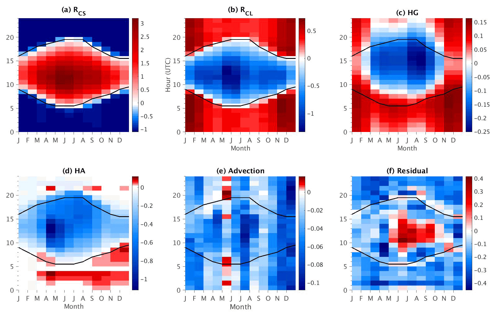
Figure 4Monthly–hourly mean values for (a) RCS, (b) RCL, (c) HG, (d) HA, (e) Adv, and (f) the residual (i.e., difference between the model and the observations). Units on the color bars are all in ∘C h−1, and their scale is different for each subfigure. The black contour line on each figure corresponds to sunrise (bottom line) and sunset (top line) approximate hours.
A diurnal cycle is pronounced for all the terms (Fig. 4). RCS contributes the most in magnitude to local temperature variations during daytime (Fig. 3a), and the other terms damp its effect by providing a negative contribution. Furthermore, all the terms are mainly driven by the solar radiation intensity during the day. The diurnal and annual cycles of the RCS (RCL) term are important, by having a positive (negative) contribution during the day, mostly dominating the temperature variations at this scale (as stated in Gaevskaya et al., 1962). The contribution of RCL on during daytime is more important during May and June and finds its minimum for December and January, when the solar radiation is weak, thus preventing clouds from strongly reducing it. Further, a maximum negative (positive) contribution to temperature variations in RCL (RCS) is found during the late mornings for all the months, cooling (warming) the surface with a maximum mean value of −1.3 ∘C h−1 (3.2 ∘C h−1) in May and June at 10:00 and 11:00 UTC.
In addition, the HA term plays an important role in temperature variations for spring and fall seasons, when there is an increase in hourly solar radiation (Fig. 3a and 4d). These two seasons are characterized by an important contribution of this term in the late morning and the afternoon, in particular during spring, with an hourly maximum averaged contribution of −1.1 ∘C h−1. The difference between day and night for the HA term is the largest during these months when the MLD can reach high values in the afternoon due to increased turbulence. For winter, its contribution is minimal due to the low development of the MLD. This result is in contrast with the negative (and very low) contribution of the HG term, which is maximal in summer in the afternoon with an average smaller value of −0.25 ∘C h−1 when the near-surface temperature is the highest and thus strengthens its cooling action during daytime. An opposite effect is found in winter when the ground is usually warmer than the surface, yielding to a positive contribution (Figs. 3a and 4c). The advection term does not present a strong monthly–hourly cycle compared to the other terms, although one can distinguish a mean negative action (still very low) to local temperature variations at all seasons with a mean minimum in July in the afternoon of −0.12 ∘C h−1, as shown in Fig. 4e.
Lastly, the residual, defined as the difference between the model (sum of all terms) and the observations (i.e., ), also has a seasonal variability and is mainly negative, but a minimum difference of −0.45 ∘C h−1 between the two datasets is found in April between 07:00 and 09:00 UTC, which is partly related to the negative increase in the HA term at that time. This is due to the important absence of latent heat flux data especially for this month, which implies an increase in the bias when τa is estimated (see Table 1 and Appendix A). Nevertheless, during the months when solar radiation is strong, the residual reaches positive values (with a maximum value around 0.4 ∘C h−1 in June in late morning) but remains a low overestimation. These values for the residual are low compared to the magnitudes of RCS, but it remains almost at the same order of magnitude as the RCL and HA terms, and a good correlation in a diurnal cycle approach is found. Generally, this hourly mean residual could also be due to the simplifications and assumptions made in the model, undersampling, and energy imbalance.
Focusing on the transition periods (sunrise and sunset, black lines in Fig. 4), the residual presents low values at these times. Indeed, there is a slight underestimation of the model of about −0.13 ∘C h−1 for some months (e.g., February) at sunrise hours, whereas a low overestimation with close-to-zero residual mean values is found for May and June. For the sunset, a similar behavior is found (with very similar values for the residual term). Therefore, a good agreement is found between the model and the observations for these specific hours.
In this section, a random forest (RF) evaluation (James et al., 2013; Manish, 2016; Brownlee, 2016; Loh, 2002) is carried out at different timescales to estimate the relative weight (i.e., importance) of each term in temperature changes according to the hour, month, or season. This machine learning method consists of bootstrapped–aggregated decision trees, a method that combines and gathers together the results of these trees to construct more powerful prediction models.
One of the most impressive features of RF is used here, which consists of the ability to provide a fully nonparametric estimation of the importance of each term (or predictor) for the model. One of the main advantages of this method is that it allows us to cover not only the impact of each term individually in the model but also the multivariate interactions with other predictors. Here, the model (i.e., ) has already been developed and defined as the sum of five terms. Therefore, to determine the importance of each term, the input data (the five terms) in the RF method are trained to predict the modeled temperature changes (), and so here the output of the RF method is still . To know more on how the hyperparameters are tuned, how the data are split up into training and testing, and further information on the RF method, please refer to Appendix B.
Other approaches to estimate the predictor importance (e.g., simple squared marginal correlations method, squared standardized coefficients) do not give reliable results when the problem involves correlated predictors (Grömping, 2007). Additionally, this method is used as a result of the nonlinear relationship between each separated term and the model (not shown), which does not yield to an estimation and quantification on how each process at the surface affects the temperature variations, an approach suggested and used by Miller et al. (2017), who estimated the response and importance of some surface processes (such as Flat and Fsens) to the forcing radiative terms in Summit, Greenland.
4.1 General behavior of the weight of the different terms
Firstly, the random forest method is used to establish which term dominates the temperature changes in the model () during day and nighttime. The predictor importance estimate value is defined as the sum of the mean square error (MSE) of each term averaged over all decision trees used and normalized by the standard deviation taken over the trees. This principle consists of permuting the values of a term – predictor – in the decision trees where this term was left out-of-bag and assessing how much worse the MSE becomes after the permutation (James et al., 2013, Chap. 8). Thus, the larger this value, the more important the term. This importance estimation feature from the random forest method has been previously used to calculate the variable importance in different datasets for many applied problems in sciences or health fields for both regression and classification studies (e.g., Archer and Kimes, 2008; Genuer et al., 2012; Strobl et al., 2007).
Figure 5a and b present the predictor (i.e., each term involved in ; see Eq. 2) importance estimate value for daytime and nighttime, respectively. Figure 5a corroborates that RCS is the most important term, followed by RCL and then HA, whereas HG is the least important term in the model developed for the timescale considered. Next, Fig. 5b illustrates that RCL dominates hourly temperature variations during nighttime, followed by HG and RCS. These results agree with Kukla and Karl (1993), who suggested that the key regulator of nighttime warming temperatures is downward thermal radiation when cloudy cases are presented, an effect that is damped most of the time by the radiative cooling effect of the ground.
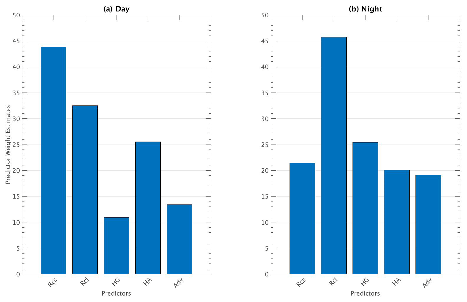
Figure 5Predictor importance estimates obtained by the random forest method for (a) day and (b) night. The abscissa in both cases represents each predictor (or term) of the model, and the y axis represents their importance (unitless) defined as the sum of their mean square error when permutation in the decision trees is done.
4.2 Diurnal cycle of the weights
The importance estimation previously calculated for both day and nighttime periods considers all the processes occurring during each case and thus gives a global importance estimation. In order to separate the influence of each term on hourly temperature variations, an importance estimation value is performed for each hour independently. Figure 6 presents the results of this method for each season. This diurnal cycle is estimated by applying the random forest to each hour separately. As expected (and previously exposed), for all the seasons RCL is the term dominating during nighttime, just after sunset, and before sunrise (indicated by vertical dashed lines in black).

Figure 6Diurnal cycle of the predictor importance estimate for each term of the model, for (a) winter, (b) spring, (c) summer, and (d) fall. Same colors as in Fig. 2a and b. Vertical dashed black lines are for sunrise and sunset mean hours.
After sunrise, the surface heating produced by the sun in the early morning enhances a high growth rate in the temperature variations, whose effect makes RCS the dominant term driving at those hours of the day for all seasons, except for winter. For this latter season (Fig. 6a), the growth rate of RCS is almost the same as that of RCL, and thus it does not expose an important estimation value. This effect is due to the weak mean solar zenith angle (SZA) for this season, and the surface heating by the sun in clear-sky conditions is not strong enough to dominate temperature variations. On the contrary, RCL importance reaches its minimum just after sunrise and before sunset, where, depending on the season, either RCS or HA is the main term controlling temperature variations.
A shift in importance between RCL and RCS occurs during the rest of the day for the four seasons of the year. This effect is explained by the variation in the data for these two terms: RCS standard deviation for a given hour or season is weak, and thus its influence to explain the difference between one day and another at a specific hour remains minimal; it is not a strong predictor at the diurnal cycle scale, especially in the summer and spring (Fig. 6b and c, respectively) when other variables will modulate temperature variations. On the other hand, RCL turns into the main modulator of for all the seasons due to its strong standard deviation for a given hour or season, reaching its maximum importance in summer (Fig. 6c). Therefore, the hourly temperature variations are more sensitive to cloud changes rather than solar radiation, which does not vary significantly for a specific hour from day to day.
Concerning the other terms, HA importance grows along the day. Its variation is greater than that of the other terms, making it the second most important modulator most of the time (except for autumn, Fig. 6d). Its contribution is weak in winter due to the lack of solar radiation and vegetation, whose absence will diminish the turbulent heat fluxes measured at the surface, along with a weak MLD. Note that it sometimes becomes the most important term in the late afternoon just before sunset. This is explained by an increase in instability of the ABL enhanced by a large boundary layer and near-surface temperature gradient (i.e., the difference between TMLD−T2 m reaches its maximum; see the third term of the right side of Eq. 7) in the late afternoon (not shown), which is generated by the increase in turbulence fluxes near the surface.
Regarding the Adv term, it shows an important weight in some hours in the late afternoon in winter, which makes it the term controlling average hourly temperature variations at that time (then it is HA that becomes more important). In summer (Fig. 6c), it presents an important increase as the day goes on, similar to HA after 10:00 UTC, but HA is even more important thanks to a development of turbulent heat fluxes at the surface in the late afternoon. Adv becomes the second most important modulator during nighttime before sunrise for all seasons except summer. A thermally induced circulation linked to the urban heat island set up in Paris is probably at the origin of this importance: this circulation is likely to create a greater variation in temperature some nights when cooler air from rural areas is advected to warmer zones towards the city center. The SIRTA observatory, located in a suburban area 20 km from the center of Paris, could be regularly affected by this modulation of circulation. Indeed, in this area the two predominant winds come from the S-E regime (the Siberian High) bringing mostly cold air temperatures and the S-W regime (air masses coming from the Atlantic Ocean) with warmer and more humid air (not shown).
Figure 6 supports a clear and reliable estimation of the importance of each term split into seasons for every hour of the day, which is not seen by estimating the diurnal and annual cycle contribution of each term to temperature variations (see Sect. 3). Indeed, depending on the hour of the day (and thus the state of the atmosphere), one term will become important over the rest, and temperature variations will be more sensitive to its change even if its contribution in terms of magnitude remains smaller compared to other terms. For instance, RCS absolute contribution during nighttime is higher than that due to RCL (Fig. 3b), and yet the latter is more important during nighttime due to its seasonal and hourly (not shown) contribution variability to .
4.3 Validation of the random forest method
However, this machine learning method is generally used in other studies to train and to have better estimations of a particular model. In order to validate the random forest method skill on predicting new observed temperature variations, the method is used to predict (rather than as done to estimate the weight of each term in Sect. 4.1). The output for this case is called . A comparison between (i.e., the linear sum of the five terms) and the new is done; the results of this validation are shown in Fig. 7. Indeed, the scatterplot before performing the random forest method () shows the distribution of values between the observations and the model (i.e., vs. , blue points) as found in Fig. 2c. Then, when the random forest method is performed and the data are trained based on (instead of ), better predictions are obtained between and (orange points), and the correlation coefficient has a higher value (0.94). In such a case, the RF method gives better estimations of temperature variations, but the retrieval of the function used to obtain these results is not available. Nevertheless, this result validates considering temperature variations as the sum of the five terms to estimate their importance using the RF method (when it is used to predict the modeled temperature variations).

Figure 7Scatter plot of as a function of the developed model before applying the random forest method (blue circles) and as a function of the model trained after the RF method is applied (orange circles).
Section 4 shows that clouds are the main modulator of solar radiation on hourly temperature variations during the day (and the main contributor during the night). Knowing how and in what measure each term contributes to temperature variations, a deeper analysis is performed in this section in order to better understand the role of clouds. This analysis is performed by considering other variables available in the SIRTA-ReOBS dataset to characterize both the atmosphere and the clouds.
In the following, only cloudy cases are considered. These cases are identified based on a criterion on the absolute value of cloud radiative effect (CRE) that must be higher than 5 W m−2 in SW and LW (Chiriaco et al., 2018) during daytime, whereas for nighttime only LW is considered for this criterion. The SWCRE (and LWCRE) is calculating following Eq. (11):
According to this threshold, cloudy conditions correspond to 82 % of the total cases from January 2009 to February 2014, and unique-clear-sky conditions represent the remaining 18 %.
5.1 Daytime analysis
Since the RCS term dominates during daytime, the ratio of divided by RCS is created to estimate how much these two terms are driven by the solar radiation: when this ratio is close to 1, it means that the variations in temperature are the ones that would be expected in clear-sky conditions with no other modulators, and when this ratio deviates from 1 it means that the temperature variations are damped or enhanced by the other terms. The ratio is also estimated, of which the distribution (not shown) has two peaks, one between −0.5 and −1 and one slightly negative with a tail in positive values. Thus, three bins are created from the highest cooling effect to the warming effect: (i) (bin 1), (ii) (bin 2), and (iii) (bin 3). The cases with negatives or values of RCS very close to zero (10 % of the cases), which occurred in early morning and late afternoon, are excluded since they affect the sign of the distribution or give divergent values. This histogram along with the one used in Sect. 5.2 are presented in Appendix C.
Figure 8a shows the values of the observed temperature variations divided by RCS, and Fig. 9 shows the distribution (represented as box-and-whisker plots) of different relevant meteorological observations available in the SIRTA-ReOBS dataset, for each bin created, split into seasons for daytime. To add cloud information, lidar data are also considered, but because they are not available all the time, and in particular when it is raining (see Sect. 2.2), they are presented as additional boxplots (light color ones) that correspond to the lidar sampling (whereas the dark-color boxplots are for the total cloudy sampling). This difference of sampling mostly affects the first two bins when clouds have a cooling effect, for which both the occurrence and the amount of precipitation are the highest (not shown). Lidar SR(z) histograms presented in Fig. 10 are estimated by cumulating all lidar SR(z) observations available for one bin and one season in particular. The red horizontal lines on each histogram correspond to low- (P>680 hPa), mid- ( hPa), and high-level (P≥440 hPa) cloud limits (Chepfer et al., 2010; Chiriaco et al., 2018). Note that a noise bin is presented here, which is simply the sum of the −999 and −777 bins that correspond to noisy and non-normalized profiles (see Sect. 2.2).
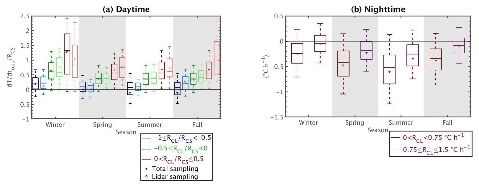
Figure 8(a) daytime values for the four seasons for three bins: in blue, in green, and in red. Dark-colored boxplots with the mean represented as “∗” correspond to cases when all meteorological variables are available at the same time (without considering lidar availability), whereas light-colored boxplots with “∘” as their mean value represent the sample when both all meteorological variables and lidar profiles are available simultaneously. (b) nighttime values for two RCL bins: 0 ∘C h−1 < RCL<0.75 ∘C h−1 in maroon and ∘C h−1 in purple. Distributions are represented by box-and-whisker plots, where the boxes indicate the 25th and the 75th data percentiles, the whiskers indicate the 5th and 95th percentiles, the middle line represents the median, and the ∗ or ∘ is the mean. Negative and close-to-zero values are removed (see text for further information).
5.1.1 Case with strong cloud cooling effect – bin 1
Figure 8a shows that the values of temperature variations (normalized by RCS) are the lowest for clouds having the most cooling effect (bin 1 in blue) for all the seasons. In winter this ratio stays mostly positive (temperature increase in 1 h) but less than 0.5 (less than half the increase that could be reached if the sky were clear), and it can become negative during summer and fall, i.e., the warming induced by RCS can be counterbalanced by the clouds in these seasons. In addition, the cloud cover is almost total, and the radiative effects are strong, as seen in Fig. 9d, e, and f. In addition, the seasonal variability of SWCRE is directly related to the seasonal variability of , and not (or only slightly) to the seasonal variability of cloud properties, since the ratio remains almost constant during the entire year (not shown) and cloud cover presents the highest mean values (Fig. 9d).
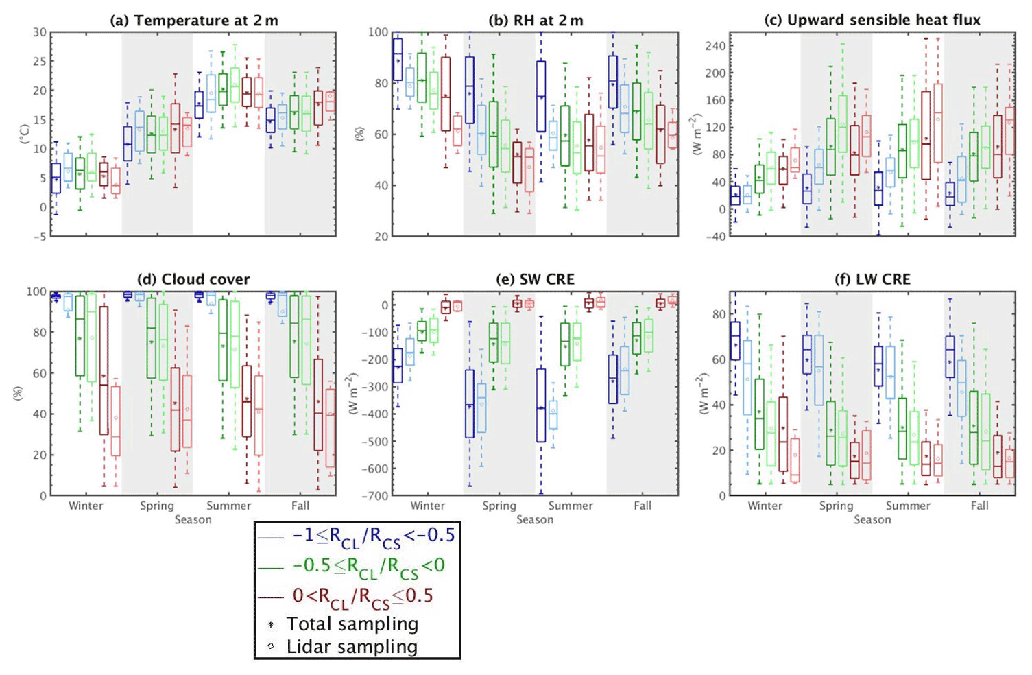
Figure 9Daytime values for (a) temperature, (b) relative humidity, (c) upward sensible heat flux at 2 m, (d) cloud cover retrieved from a sky imager, and (e) shortwave and (f) longwave cloud radiative effect. Colors and boxplots follow the same definition as in Fig. 8a.
The light blue bin is the same as the dark one except for lidar sampling, i.e., for non-rainy cases exclusively. Indeed, lower RH values (Fig. 9b) favor lower precipitation occurrence (not shown), higher amount of Fsens (Fig. 9c), and higher (i.e., less negative) values of SW CRE (Fig. 9e) for the lidar sampling compared to the total one. Logically, lower LWCRE is found for the lidar sampling. As expected, temperatures are higher for the lidar sampling for all the seasons except summer, as shown in Fig. 8a, along with a more frequent negative temperature variation (Fig. 8a). For this sampling that excludes rainy cases, both higher and lower values of SWCRE are found for spring rather than for summer (Fig. 9e): the minimal value is around W m−2 for spring, whereas for summer it is W m−2 (a situation not captured by the total sampling where summer has a lower value of SWCRE than spring). Figure 10b shows that low- and high-level clouds are more frequent for spring than for summer (Fig. 10c), and thus stronger negative values of SWCRE are found for spring. Then, the important presence of mid-level clouds with a high value of lidar SR(z) (>80) spotted in summer in Fig. 10c is potentially the cause of the strong negative values of SWCRE despite the very low presence of other clouds. These strong and negative SWCRE could be associated with a presence of nimbostratus clouds, due to the high SR detected for lidar, clouds which are more likely to form in summer because of the strong convective systems developed during that time due to higher surface temperatures. In addition, despite the strong negative values of SWCRE for this bin for all seasons, near-surface temperatures are not so low (Fig. 9a), partly due to the high LWCRE values (Fig. 9f) that slightly dampen the strong SWCRE.
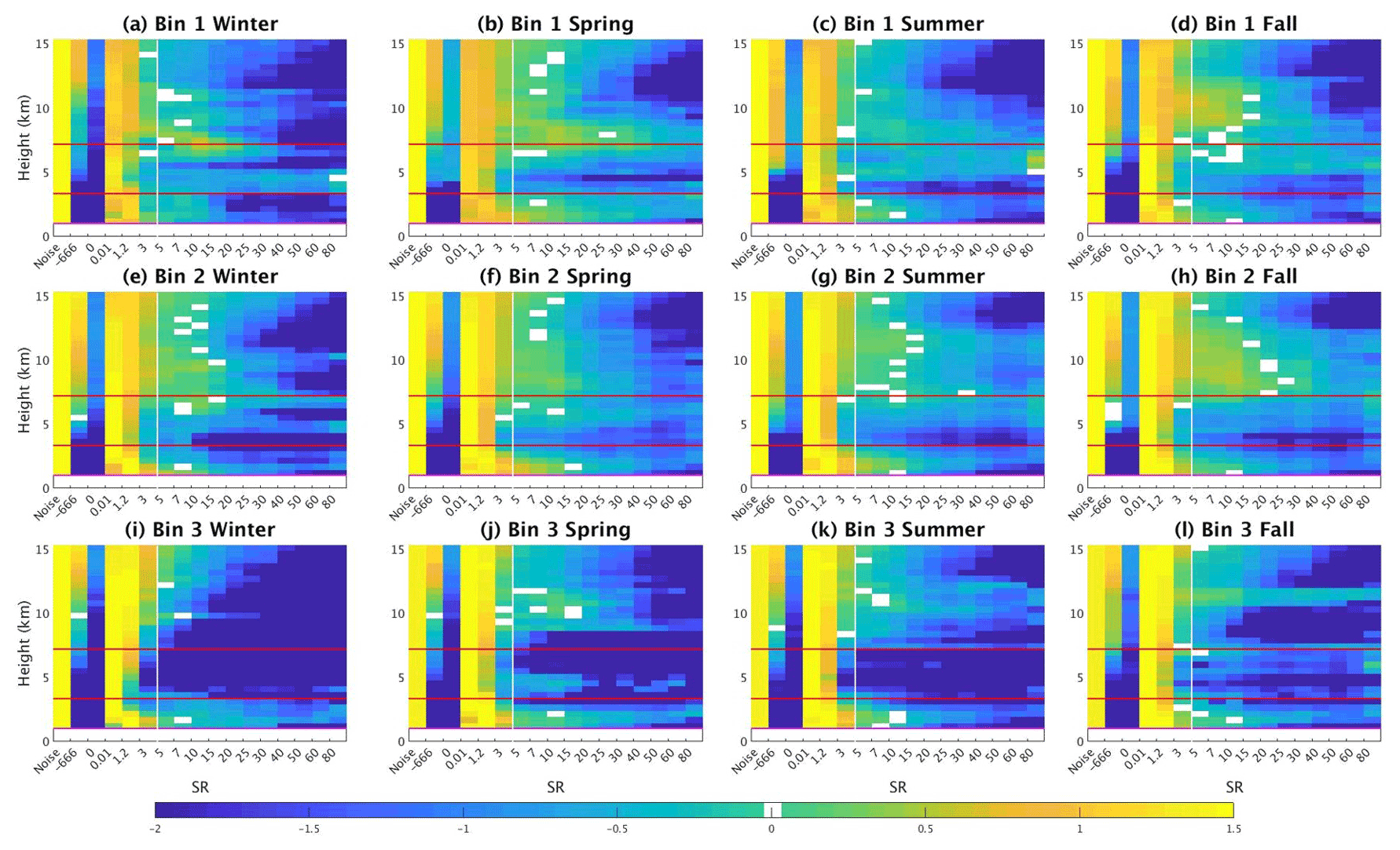
Figure 10Lidar scattering ratio (SR(z)) histogram obtained by cumulating all lidar observations during daytime for bin 1 (a–d), bin 2 (e–h), and bin 3 (i–l) for winter (first column), spring (second column), summer (third column), and fall (fourth column). The color bar is the logarithm of the percentage of occurrence (the sum of one level is equal to log 10100 %); lidar data showed in each subplot start above the instrument's recovery altitude (z=1 km); the red horizontal lines represent the limits of low-, mid-, and high-level clouds, and the white vertical line shows the threshold of cloud detection (SR(z)=5).
Some differences in cloud presence can be detected in Fig. 10a–d for the first bin. For the fall season, the SR(z) histogram in Fig. 10c exhibits an important presence of high-level thin clouds (especially above 8 km), along with mid-level thick clouds. Figure 10b also presents an important presence of high-level clouds in spring but within a smaller vertical range ( km) compared to fall. Indeed, one reason explaining the presence of these high-level clouds at these two transition seasons could be the convergence of a warm air with a cold air mass (which occurs more often in spring and fall), where the lighter warm air rises up to several kilometers from the ground and could form some cirrus clouds. In addition, spring exhibits high amounts of low-level thick clouds (SR>40) that are not detected the rest of the year, which could correspond to the moments just before a storm is set. Indeed, the highest precipitation rates are found for this season (not shown), and the cloud cover minimum in Fig. 9d for the lidar sample is 90 % (the highest among the other seasons), and fewer clear-sky conditions are found ().
5.1.2 Cases with weak cloud radiative effect: cooling or warming
When RCS becomes dominant with respect to RCL (bins 2 and 3), temperature variations are positive most of the time, especially in winter (Fig. 8a). In comparison with the first bin, the air becomes drier (higher sensitive heat flux and lower RH, Fig. 9b and c), which agrees with less cloud cover (Fig. 9d), and lower LWCRE and less negative SWCRE (Fig. 9e and f). Figure 10 shows fewer differences between bin 1 and bin 2 (RCL<0) than between bin 2 and bin 3 (RCL>0) because this figure only considers non-rainy situations, and in Sect. 5.1.1. it is noted that there are important differences between the two samplings (total and non-rainy) for bin 1 for most of the variables. This difference between the two samplings is weaker for bins 2 and 3, despite its existence in winter and fall. Figure 10 is thus more representative of the full sampling for these two bins than it is for the first bin.
For the lidar sampling, LWCRE in winter and fall is slightly higher than for the two other seasons for the second bin (Fig. 9f). This is partly due to the presence of high-level thin clouds (), such as cirrus, detected in the histograms of SR(z) for this bin in Fig. 10e and h for these two seasons, which is slightly more than for spring and summer.
In bin 3, the absence of mid-level clouds and the lower occurrence of high clouds compared to bin 2 is obvious, while the difference for low-level clouds is not clear. This is consistent with lower LWCRE (Fig. 9f) but not necessarily with the very low values (i.e., close to zero) of SWCRE observed for bin 3 (Fig. 9e). The SWCRE values close to zero are explained by the fact that most of the hours corresponding to this bin 3 coincide just after sunrise (not shown), when solar radiation is still weak, thus explaining that . These low SW and LWCRE values for the lidar sampling also correspond to low mean cloud cover (Fig. 9d) and thus a lower number of clouds are detected by the SR(z) histograms (Fig. 10i–l). Note that some of the SWCRE values are even positive, revealing that , an effect observed when the direct part of solar radiation is not fully attenuated and when some diffuse radiation reaches the surface in addition to the direct flux, radiation which is strengthened by scattering processes in clouds and atmospheric particles. This effect thus increases observed radiation beyond a respective clear-sky scenario, and it mostly happens in winter (but could occur the rest of the year) in early morning and/or late afternoon hours when the solar elevation angle is weak (Stapf et al., 2020; Wendisch et al., 2019). This distribution towards early morning hours explains that despite the high values of the ratio between temperature variations and RCS (Fig. 8a) and lower cloud cover and cloud effects, near-surface temperatures are not always maximal for this bin (these maximal temperatures happen only for spring and fall).
5.2 Nighttime analysis
During nighttime, a similar procedure is followed to analyze and characterize different meteorological variables under different cloudy conditions. Since RCL is the term dominating and controlling temperature variations (Sect. 4) and since RCS is constant, it is not necessary to divide it by RCS. Thus, two bins are created from the PDF of RCL: ∘C h−1 and ∘C h−1. During nighttime there is no SW radiation, so clouds always have a warming effect on near-surface temperature. The distribution of for the two bins created for all the seasons is presented in Fig. 8b. Figure 11 shows the same meteorological variables shown in Fig. 9 but for nighttime cases. Cloud fraction profiles are not shown because the lidar does not operate during nighttime.
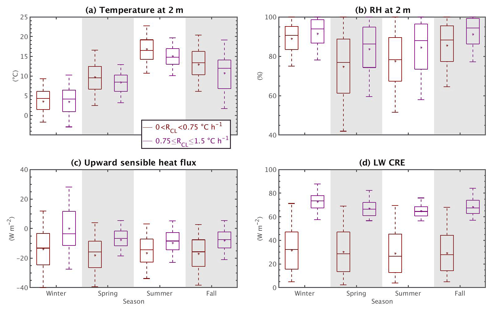
Figure 11Nighttime values for (a) temperature, (b) relative humidity, (c) upward sensible heat flux at 2 m, and (d) longwave cloud radiative effect. Colors and boxplots follow the same definition as in Fig. 8b.
Figure 8b shows that the temperature variations are generally stronger for the first bin than for the second bin; i.e., the negative temperature variations induced by longwave cooling during nighttime are damped when the effect of clouds is stronger. This agrees with what is expected since, at hourly timescales, clouds are the most important factor in modulation of temperature variations during nighttime (see Sect. 4). As expected, the second bin has stronger LWCRE values (Fig. 11e). The effect of clouds seems enhanced when cool and moist air is present over SIRTA (Fig. 11a, b). More details for each bin are given in the following subsection.
5.2.1 Case with weak cloud warming effect
For the first bin ( ∘C h−1), LWCRE presents a wide range of values going from 5 up to 75 W m−2 with no seasonal variability detected (Fig. 11d), and yet temperatures are the highest for this bin (Fig. 11a) except in winter. As expected, upward sensible heat flux is negative due to surface cooling most of the time, as values of are predominantly negative (Figs. 11c and 7b, respectively), with drier air conditions since RH has the lowest values for all the seasons (Fig. 11b).
5.2.2 Case with strong cloud warming effect
The temperature distribution has the lowest values for all seasons (except spring) for the category of clouds that have the strongest warming effects (second bin, in purple in Fig. 11a). This category of clouds is tightly linked to strong LWCRE ranging from 55 up to 90 W m−2 (Fig. 11d). These low temperatures could be associated with situations when the incoming air masses are colder, which is linked to large-scale situations (Pinardi and Masetti, 2000; Wang et al., 2005). Note that here hourly temperature variations are studied, and indeed on multi-day timescales, it is the large-scale atmospheric processes that determine the daily temperature value to the first order.
Finally, the distribution of sensible heat flux is positive in winter, with values reaching up to 40 W m−2 (purple boxplot, Fig. 11c). These unusual and positive values during nighttime are explained by the presence of a strong stable atmospheric layer, where near-surface temperatures are the lowest except for spring (Fig. 11a), and the atmosphere is warmer at higher altitudes since clouds contribute to warming the most at this time, and therefore a positive upward sensible heat flux develops. Similar behavior was also previously found by Miao et al. (2012) in Beijing during nighttime in cloudy conditions, where sensible and latent heat fluxes were close to zero due to the presence of a stable atmospheric layer, especially in winter when the sensible heat flux is found to be slightly greater than the latent heat flux. Indeed, almost half of temperature variation values are found to be positive for this season, as illustrated in Fig. 8b. Along with the positive upward sensible heat flux found, higher temperatures are found for this bin, which is not seen in the other seasons where the sensible heat flux is close to zero or mostly negative and temperatures are higher for the first bin (cloud with a low warming effect).
The European climate and most temperature anomalies are affected not only by the circulation of large-scale air masses (such as the NAO or blocking regimes) but also by smaller-scale processes such as cloud radiation and surface–atmosphere interactions located within the atmospheric boundary layer. In this paper, a method is developed and evaluated to quantify each process that affects hourly 2 m temperature variations on a local scale (near Paris), based almost exclusively on observations. The method exhibits good accuracy and is able to quantify the realistic diurnal and monthly–hourly cycles of each term involved well, especially in summer when statistics are the best. The clear-sky radiative term represents the biggest positive (negative) contribution during daytime (nighttime), with values reaching up to 4 ∘C h−1 (−1.7 ∘C h−1), whereas clouds cool (warm) up to −3.7 ∘C h−1 (1.4 ∘C h−1). The atmospheric heat exchange becomes predominant in the late afternoons when turbulent fluxes develop due to the increase in atmospheric instability. Some of the biases found are due to the difficulty of the model to reproduce smaller-scale processes such as the cold pool events well.
The use of a random forest analysis makes it possible to identify which term dominates over the others. Clear-sky radiation most influences the 1 h temperature variations during the day, whereas the cloud radiation has the most influence during the night followed by the ground heat exchange term. Nevertheless, separating the dataset into hours and seasons shows that the cloud radiation effect becomes predominant in several hours for all the seasons because it presents a greater variation in its hourly values than the clear-sky radiative effect, especially in spring and summer during daytime when more local cloud cover variability occurs. This cloud dominance is still found despite the fact that the clear-sky radiation magnitudes are the highest on a monthly–hourly scale. Temperature variation is then more sensitive to cloud changes within an hour rather than the large contribution of clear-sky radiation which mostly dominates the early mornings when surface heat fluxes are not yet developed. The other terms remain important as there are times when some of them modulate temperature variations, especially the turbulent heat fluxes in the late afternoons. These terms also remain necessary to obtain the best coefficient estimator between the directly measured observations and the method developed.
To better understand the importance of clouds on temperature variations at this scale, a deeper analysis is performed partly based on lidar profile observations. The atmosphere presents a high amount of cloud fraction detected by both the lidar and the sky imager during the daytime, which correlates well with the strong cooling contribution found for the cases when clouds have a strong cooling effect. Indeed, an important presence of mid-level thin and thick clouds is spotted for all the seasons (except spring) for these cases. These thick clouds could correspond to nimbostratus, which are very opaque and often produce continuous moderate rain, but the lidar detects them just before the rain starts. Indeed, temperatures at this time are very low, which contributes to these clouds forming since they usually form ahead of a warm front. On the contrary, a weak cooling effect is predominantly associated with low- and high-level thin clouds for all seasons. Situations with daytime positive cloud radiative effect occur when the atmosphere is close to clear-sky conditions and corresponds to low- and high-level thin clouds mostly in early morning and late afternoon. In addition, situations with weak cloud effect (either negative or positive) coincide with an important amount of high-level thick clouds for all the seasons (except winter) whose LWCRE is high, but SW clear-sky radiation controls temperature variations (Fig. 8a, bins 2 and 3). These high-level clouds are more present in weak cloud cooling and warming effects (bins 2 and 3) than the times of strong cooling effect (bin 1). Overall, a dominance of mid- and high-level clouds at the SIRTA observatory is detected for all cases. The dominant presence of this specific type of cloud is linked to the geographical position of the SIRTA observatory since it is located in a zone where warm and wet air coming from the Atlantic Ocean can nudge against the cold and dry masses of air coming from the Siberian region. This encounter of air masses (whether it is the warm air that encounters cold air or the opposite) tends to form mostly high-level clouds. Similar behavior has been found by Chakroun et al. (2018) during nighttime and Mariotti et al. (2015) over the Euro-Mediterranean area where the variability of cloud fraction (CF) is driven mostly by the encounter of two different air masses coming from northern Europe and southern Africa. During nighttime, even when clouds have a positive important radiative effect, temperatures are low and they are more controlled by large-scale processes since surface turbulent fluxes are low and there is no shortwave radiation most of the time. Since neither cloud fraction variable nor lidar data are available during nighttime, no information about the percentage of cloud presence can be known, yet variability on LWCRE is still found between clouds whose warming effect is weak and those whose warming effect is strong. This LWCRE variation is controlled by the presence of clouds to the first order, but it could also be due to the sensitivity of LW radiation arriving at the surface to the presence of atmospheric gases and aerosols and not only to cloud radiative properties, as shown previously by Dufresne et al. (2002), Satheesh and Krishna Moorthy (2005), and Kushta et al. (2014). In addition, the strong stability of the atmosphere at night creates positive sensible heat flux when clouds have the warmest effect on temperature variations.
The approach developed in this study is innovative because it is predominantly based on observations. It opens several perspectives on the possibility for continuing work: (i) use of the approach in combination with weather regimes to better relate the small-scale processes to the large-scale atmospheric dynamics, (ii) application of the approach to other locations to understand the spatial variability of the results and how specific local conditions affect each of the terms involved in near-surface temperature variations, (iii) identification of the moments when one term becomes predominant over the rest by integrating the time into larger scales (such as weekly and monthly), and (iv) estimation of how well these estimations are represented in the present and future climate simulations to evaluate models and/or understand the evolution of the different terms in a warming climate. Further, the ground heat exchange contribution is very site-dependent (more than the other surface terms), with different behavior in an urban environment; therefore it will be interesting to study its impact on the attenuation–amplification of maximum near-surface temperatures in periods of heatwaves.
The prognostic model used to study the temperature change at the surface, considering all the components driving the surface energy balance, can be simply written as the sum of four processes:
where R is defined as the radiative forcing term, HG as the ground heat exchange term, HA as the atmospheric heat exchange term, and Adv as advection. Each of these terms represents a process involved in the variation in near-surface temperature and can be calculated using different measured and available variables as follows:
where T2 m is the near-surface temperature, t is the time, α is a coefficient characterizing the form of the temperature profile in the boundary layer, ρ is the average air density of the boundary layer, cp is the specific heat of air, MLD is the height of the boundary layer, ΔFNET is the net radiative flux at the surface, Ts is the temperature in the ground at 20 cm depth, TMLD is the temperature at the top of the boundary layer, u10 and v10 are the zonal and meridional wind components, respectively, at 10 m above the ground, x is the zonal wind component towards the east and y is the meridional component wind towards the north, and τs and τa are defined as relaxation timescales for heat exchange processes in the ground and the atmosphere, respectively.
Before explaining how each term is estimated, considerations are necessary about the stability of the atmosphere and related temperature profiles. Note that these assumptions will not affect the physical behavior of the developed method; they are made in order to have a more quantitative treatment of the study.
Temperature near the surface and its behavior in lower layers are mostly driven by the quantity of net radiative flux arriving on it, which also depends on what moment of the day the temperature is observed; thus, it is important to differentiate day and night. During the first case mentioned, radiative flux is significant as a result of solar incoming flux radiation (shortwave radiation), and the vertical temperature profile will depend on the amount of this radiative flux (among other components). In the absence of any incoming shortwave radiation, which corresponds to nighttime, clouds and other processes control temperature variations at the surface and its vertical profile.
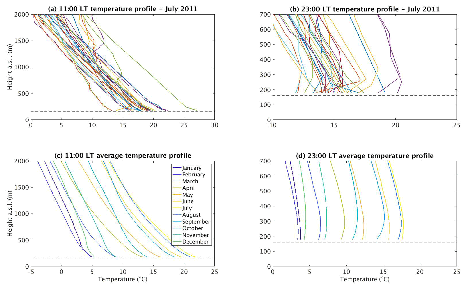
Figure A1Temperature profiles at 11:00 (a) and 23:00 LT (b) for July of 2011, and monthly averaged temperature profiles from 2003 to 2017 at 11:00 (c) and 23:00 LT (d) in Trappes. The temperatures at each altitude are retrieved from radiosoundings launched twice a day at the mentioned hours. The horizontal dashed line represents the altitude above sea level where the Trappes observatory is located, which is 160 m.

Figure A2Hourly evolution of observations (a), R term (b), HG term (c), HA term (d), and Adv term (e). Gaps in (d) are caused by the absence of MLD data at that moment.
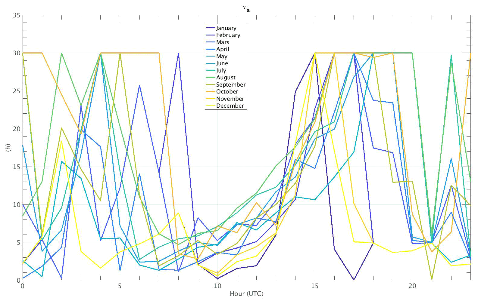
Figure A1 confirms that the planetary boundary layer (PBL) is on average unstable during daytime and stable during nighttime in the area of study. This figure is built from twice-daily radiosounding (at 11:00 and 23:00 local time) observations available in the SIRTA-ReOBS file from a METEO-France station located in Trappes (48.77∘ N, 2.01∘ E), 16 km away from the SIRTA observatory, to retrieve (every 15 m) the temperature and pressure up to 15 km above the ground. Figure A1a and b provide an overview of temperature profiles retrieved from these radiosoundings at 11:00 and 23:00 LT, respectively, for July of 2011 (each color represents a day of the month). Then, the monthly mean temperature profiles from 2003 to 2017, each month represented as one color, are plotted in Fig. A1c and d. As expected, the temperature decreases from the surface to the atmosphere in both daytime panels (Fig. A1a and c), and a temperature inversion occurs at lower layers in nighttime for the night cases (Fig. A1b and d) of the monthly mean.
This said, a daytime and a nighttime equation are used to parametrize the temperature profile in the surface layer (SFL).
For the daytime approach, a linear temperature profile is established as follows:
where β is the temperature gradient, negative during the day.
For the stable nighttime case, the temperature profile can be defined by a polynomial approach (Stull, 1988):
A shape parameter α=1.5 shows a quasi-linear behavior of the temperature profile with a weak positive gradient near the surface, fitting well with the profiles in Fig. A1c and d (not shown).
The assumption of working with an ideal gas in an isobar environment, and applying the second law of thermodynamics, yields an expression of the enthalpy as described below (Malardel, 2009; Wallace and Hobbs, 2006):
Knowing the vertical temperature profile, Eq. (A5) can be integrated all over the MLD to find the total enthalpy per square meter at a given level (assuming that the density of the air is approximately constant at lower layers).
It is found that for a nighttime case, the total enthalpy can be expressed as
By deriving this equation with the near-surface temperature and total enthalpy, the ability to assess the change in near-surface temperature per unit change in enthalpy is estimated as
For the daytime, proceeding as above, the same equation is found but for the nighttime, with the only exception that α=0.
As explained before, distinguishing between night and daytime is very important for the study due to the differences in the radiative flux arriving at the surface, which condition the behavior of the PBL (i.e., MLD) and SEB terms.
A1 Radiative term
This term is calculated as
The contribution of the radiative forcing to the temperature variations at SIRTA can be estimated by using the second law of thermodynamics, which states that the only energy a particle exchanges with its surroundings is heat. That said, it is assumed that the only heat exchanged for a particle of air in the low atmosphere with its surroundings is the net radiative flux divergence, yielding to
where is the only source of energy of the particle. By replacing ∂htot in Eq. (A7) by Eq. (A9), it is found that
with Eqs. (A10) and (A11) corresponding to night and daytime cases, respectively. These two equations described above will allow estimation of the first term of the temperature variation model at SIRTA, the radiative term. MLD is a scale of height corresponding here to the height of the PBL retrieved from SIRTA-ReOBS. This value is set at this threshold because all the turbulent processes affecting the temperature variations are found within this layer. The PBL thickness varies depending, among other processes, on the amount of solar radiation, which enhances thermal and turbulent processes, making this thickness range from tens of meters to 2 km or more. Thus, an average PBL thickness value (i.e., MLD) at an hourly or monthly scale is set (an assumption that does not affect the physical behavior of the model), as seen in Fig. A1c. Since during nighttime the boundary layer depth is difficult to estimate because of the weak turbulence due to the absence of solar radiation and its very complex dynamical system (Shi et al., 2005; Walters et al., 2007; McNider et al., 2011), a fixed value of 350 m is set (Fig. A1d). Figure A2b shows the behavior of the radiative term calculated by using Eq. (A8) assuming ρ=1 kg m−3 and cp=1006 J kg−1 K−1. A seasonal cycle is marked for this term, where during summer a peak of maximum contribution is found, whereas in winter its impact on temperature variations decreases significantly.
A2 Atmospheric heat exchange term
This term is estimated as
In this equation, τa can be calculated at equilibrium by setting the left side of the Eq. (A2) to zero and neglecting the ground heat exchange and advection terms (i.e., for the temperature not to vary, a balance between these two latter terms must be set), leading to
For the atmospheric heat exchange, . However, Flat has lots of missing values in the SIRTA-ReOBS dataset (material defection) and therefore does not allow us to perform a complete analysis for the 5 years of study. Hence, an hourly and monthly look-up table (LUT) is created to have an estimation of τa. Moreover, TMLD is not directly available in the SIRTA-ReOBS dataset. To retrieve that temperature, the mixing layer depth is first retrieved from the SIRTA-ReOBS dataset, by looking for the nearest radiosounding in time (two per day) and finding the pressure corresponding to this altitude; then it is possible to obtain the temperature at that pressure level by looking at them in the ERA5 dataset. Figure A3 shows an average τa for all the months of the year. During night, the relaxation timescale shows a higher month-to-month variability mainly due to the absence and gaps of the latent and sensible heat fluxes, which does not allow the reflection of a marked tendency of τa, whereas for daytime a more clear behavior of τa is spotted for all the months thanks to an increase in the availability of the data for these hours (not shown). Sometimes during nighttime, this relaxation time exceeds 30 h, probably because the turbulence is so weak at that time that the heat does not completely reach the surface boundary layer (SBL) established. Stull (1988) suggested that for the night cases, values of τa are on the order of 7 to 30 h, depending on the state of the SBL. Thus, values are limited to 30 h. For daytime, τa remains smaller because the turbulence is stronger thanks to convection occurring near the surface, leading to a faster communication of surface information across the lower layers.
The atmospheric heat exchange term hourly values are shown in Fig. A2d. Most of the values are negative, indicating that this term will modulate the positive contribution made by the radiative forcing term.
A3 Ground heat exchange term
The ground heat exchange term is defined as the energy lost by heat conduction through the lower boundary. This term can then be determined as follows:
On average, the near-surface temperature during daytime (nighttime) is higher (lower) than that at low depth, as has been shown previously (Al-Hinti et al., 2017; Popiel and Wojtkowiak, 2013). Hence, the assumption that the vertical profile of temperature within the ground at low depths follows approximatively the same behavior as the atmospheric temperature profile can be established, and therefore the approach adopted for the atmospheric heat exchange term (see Appendix A2) can here be implemented, to evaluate the relaxation timescale for the ground heat exchange at a depth of Hs=0.2 m below the ground. The surface is considered to be warmer than the temperature at 20 cm below the ground during the day thanks to the solar radiation arriving. The opposite happens during night, when the ground loses important longwave radiation, and it gets cold faster than Ts. Knowing the temperatures at the top of the ground (T2 m) and at 20 cm below it (Ts), the relaxation timescale results in
The soil type at the SIRTA observatory is a mix of clay and limestone (obtainable from a regionally predominant type of soil map in France; Wulf et al., 2015). The approximative values for ground density ρs and heat capacity cp,s for this type of soil are then
A mean value of τs=20 h for the daytime and nighttime cases is found. Figure A2c presents the contribution of this term to the temperature variations, which is very minor but remains important to have a better agreement between the developed model and the directly measured observations, by the fact that adding or removing some units could make a difference in estimating the correlation between the two datasets.
A4 Advection term
The advection term is estimated as presented in Eq. (A16) using the ERA5 dataset of horizontal wind components at 10 m and temperature at 2 m above the ground. The purpose of using this dataset is to have another point in each horizontal axis to calculate the transport of the mass of air in zonal and meridional directions, between the SIRTA observatory and the immediately following grid box. For the period and timescale considered, the advection term mostly plays a minor role, as shown in Fig. A2e, compared to the other terms.
A5 Observed hourly temperature variation term
The left side of Eq. (A2) is defined as
where Th is the temperature at 2 m above the surface at hour h, and Th−1 is the temperature at the previously considered hour.
Figure A2a presents the evolution of this term, denoting, as expected, a seasonal cycle. Temperature variations have stronger negative than positive values, reaching a rate of −6 ∘C h−1 or even −8 ∘C h−1 a few times in summer 2010.
The sum of all terms on the right side of Eq. (A2) is hereafter called .
In Sect. 4, the random forest method is used to determine the importance of the predictors (terms) for the near-surface temperature variations. Detailed information on how this method works is given here.
The training algorithm for random forests applies the general technique of bagging, where the key to bagging is that trees are repeatedly fit to bootstrapped subsets of the observations. The bootstrapped term refers here to randomly choosing data that can be chosen several times to build decision trees (no selection restrictions). A training dataset is chosen randomly with replacement (bootstrapping) from the original dataset to create a decision tree. In regression techniques, the training dataset correspond to about two-thirds of the total of the sample. The remaining one-third of data not used to train that decision tree are used later as testing data but also to determine the importance of a specific term (James et al., 2013). This procedure is repeated for all the decision trees used in the random forest. Finally, it is not necessary to have a validation dataset in this study because the main interest of using this machine learning is to determine the importance of the terms for the model developed, as it is known that random forest protects against overfitting by constructing training samples through bootstrapping.
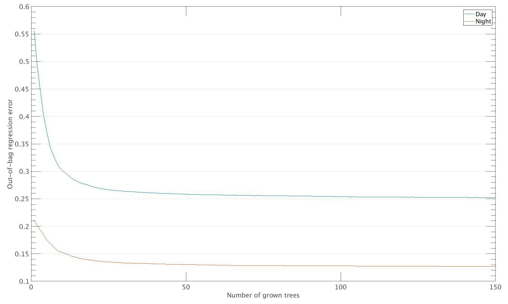
Figure B1Out-of-bag error over the number of grown regression trees for day (blue line) and night (orange line).
Some hyperparameters are tuned in order to optimize the analysis.
-
The random forest method is set to have 150 decision trees, because at that number the error converges to a small value, as seen in Fig. B1 (converging value of 0.25 during daytime and 0.12 during nighttime).
-
For the split criteria, since our model is a simple 1∘ regression, the method is set to use the mean square error (MSE) to do the split at each leaf.
The number of random features to consider at each split and the number of bootstrapped datasets used to train each decision tree in the random forest method is approximately two-thirds of the total predictors and two-thirds of the total samples, respectively (James et al., 2013).
In Sect. 5, different bins are created to analyze the specific contribution of clouds for both day and nighttime. Figure C1a shows the distribution of the ratio for daytime hours, where two peaks can be easily identified: one between −0.5 and −1 and one slightly negative with a tail in positive values. From this distribution, three different bins can be created in order to separate the effect of clouds on observed near-surface temperature variations, going from the highest cooling effect to the warming effect (rectangular semi-transparent brown boxes in Fig. C1a): (i) (bin 1), (ii) (bin 2), and (iii) (bin 3).
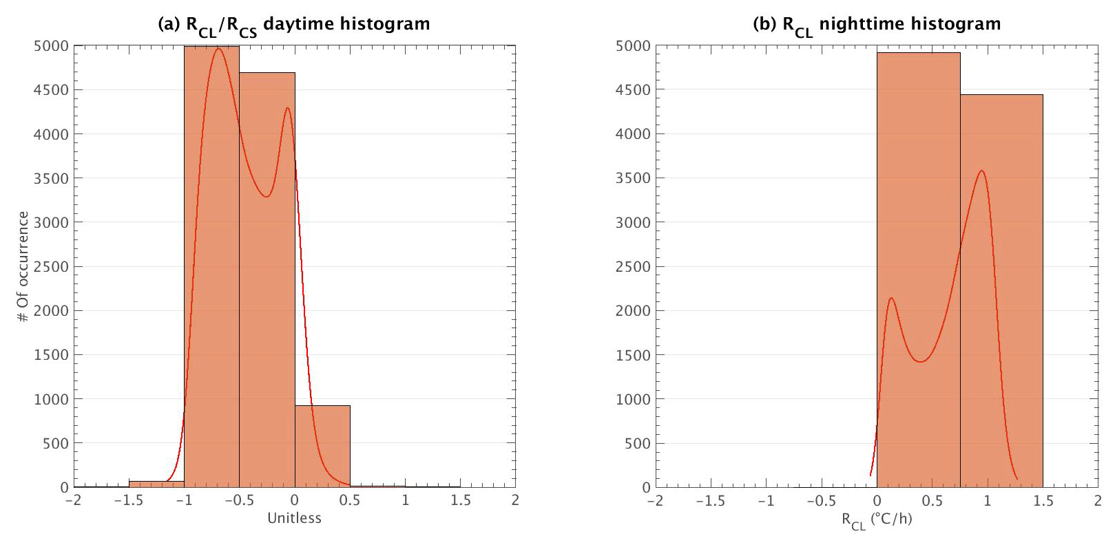
Figure C1(a) Daytime histogram of and (b) nighttime histogram of RCL. The red line in both figures represents the PDF, and the rectangular semi-transparent brown boxes represent the different bins created to analyze cloud influence. These histograms are built by considering only cloudy hours. Negative and close-to-zero values are removed for daytime hours (see text for further information).
As for nighttime cases, bins are created only considering the distribution of RCL, which is presented in Fig. C1b. Two peaks are spotted in this figure when RCL>0, and thus the following two bins are created ∘C h−1 and ∘C h−1. During nighttime there is no SW radiation, so clouds always have a warming effect on near-surface temperature.
The SIRTA-ReOBS NetCDF file used in this study is available at https://sirta.ipsl.fr/reobs.html (last access: 10 April 2021) under https://doi.org/10.14768/4F63BAD4-E6AF-4101-AD5A-61D4A34620DE (SIRTA, 2021). The advection term and the temperature at the mixing layer depth were estimated using Copernicus Climate Change Service Information ERA5-Land and ERA5 [2009–2014], respectively.
OJRM carried out the data analysis and methodology and prepared all the figures. MC, SB, and JR contributed to the data analysis, advised on methods, and performed validation and interpretation of results. OJRM wrote the manuscript with contributions from MC and SB.
The contact author has declared that neither they nor their co-authors have any competing interests.
Publisher's note: Copernicus Publications remains neutral with regard to jurisdictional claims in published maps and institutional affiliations.
The authors would like to acknowledge the Mesocentre ESPRI team at IPSL for providing storage resources and giving access to the SIRTA-Re-OBS dataset and also the SIRTA observatory for collecting and providing the geophysical variables and lidar data used in this study.
This paper was edited by Johannes Quaas and reviewed by two anonymous referees.
Al-Hinti, I., Al-Muhtady, A., and Al-Kouz, W.: Measurement and modelling of the ground temperature profile in Zarqa, Jordan for geothermal heat pump applications, Appl. Therm. Eng., 123, 131–137, https://doi.org/10.1016/j.applthermaleng.2017.05.107, 2017.
Allan, R. P.: Combining satellite data and models to estimate cloud radiative effect at the surface and in the atmosphere, Meteorol. Appl., 18, 324–333, https://doi.org/10.1002/met.285, 2011.
Allan, R. P., Liu, C., Loeb, N. G., Palmer, M. D., Roberts, M., Smith, D., and Vidale, P.-L.: Changes in global net radiative imbalance 1985–2012, Geophys. Res. Lett., 41, 5588–5597, https://doi.org/10.1002/2014GL060962, 2014.
Archer, K. J. and Kimes, R. V.: Empirical characterization of random forest variable importance measures, Comput. Stat. Data An., 52, 2249–2260, https://doi.org/10.1016/j.csda.2007.08.015, 2008.
Arkin, P. A. and Meisner, B. N.: The Relationship between Large-Scale Convective Rainfall and Cold Cloud over the Western Hemisphere during 1982–84, Mon. Weather Rev., 115, 51–74, https://doi.org/10.1175/1520-0493(1987)115<0051:TRBLSC>2.0.CO;2, 1987.
Arnold, N. S., Willis, I. C., Sharp, M. J., Richards, K. S., and Lawson, W. J.: A distributed surface energy-balance model for a small valley glacier. I. Development and testing for Haut Glacier d'Arolla, Valais, Switzerland, 42, 77–89, https://doi.org/10.3189/S0022143000030549, 1996.
Bartolini, E., Claps, P., and D'Odorico, P.: Interannual variability of winter precipitation in the European Alps: relations with the North Atlantic Oscillation., Hydrol. Earth Syst. Sci., 13, 17–25, https://doi.org/10.5194/hess-13-17-2009, 2009.
Bastin, S., Chiriaco, M., and Drobinski, P.: Control of radiation and evaporation on temperature variability in a WRF regional climate simulation: comparison with colocated long term ground based observations near Paris, Clim. Dynam,, 51, 985–1003, https://doi.org/10.1007/s00382-016-2974-1, 2018.
Bennartz, R., Shupe, M. D., Turner, D. D., Walden, V. P., Steffen, K., Cox, C. J., Kulie, M. S., Miller, N. B., and Pettersen, C.: July 2012 Greenland melt extent enhanced by low-level liquid clouds, Nature, 496, 83–86, https://doi.org/10.1038/nature12002, 2013.
Broeke, M. V. D., Reijmer, C., As, D. V., and Boot, W.: Daily cycle of the surface energy balance in Antarctica and the influence of clouds, Int. J. Climatol. 26, 1587–1605, https://doi.org/10.1002/joc.1323, 2006.
Brownlee, J.: Bagging and Random Forest Ensemble Algorithms for Machine Learning, Machine Learning Mastery, available at: https://machinelearningmastery.com/bagging-and-random-forest-ensemble-algorithms-for-machine-learning/ (last access: 18 October 2021), 2016.
Chakroun, M., Bastin, S., Chiriaco, M., and Chepfer, H.: Characterization of vertical cloud variability over Europe using spatial lidar observations and regional simulation, Clim. Dynam., 51, 813–835, https://doi.org/10.1007/s00382-016-3037-3, 2018.
Chen, T., Rossow, W. B., and Zhang, Y.: Radiative Effects of Cloud-Type Variations, J. Climate, 13, 264–286, https://doi.org/10.1175/1520-0442(2000)013<0264:REOCTV>2.0.CO;2, 2000.
Chepfer, H., Bony, S., Winker, D., Cesana, G., Dufresne, J. L., Minnis, P., Stubenrauch, C. J., and Zeng, S.: The GCM-Oriented CALIPSO Cloud Product (CALIPSO-GOCCP), 115, D00H16, https://doi.org/10.1029/2009JD012251, 2010.
Cheruy, F., Campoy, A., Dupont, J.-C., Ducharne, A., Hourdin, F., Haeffelin, M., Chiriaco, M., and Idelkadi, A.: Combined influence of atmospheric physics and soil hydrology on the simulated meteorology at the SIRTA atmospheric observatory, Clim. Dynam., 40, 2251–2269, https://doi.org/10.1007/s00382-012-1469-y, 2013.
Cherviakov, M.: Variability of Earth's radiation budget components during 2009–2015 from radiometer IKOR-M data, Geophys. Res. Abstr., EGU2016-9611, EGU General Assembly 2016, Vienna, Austria, 2016.
Chiriaco, M., Bastin, S., Yiou, P., Haeffelin, M., Dupont, J.-C., and Stéfanon, M.: European heatwave in July 2006: Observations and modeling showing how local processes amplify conducive large-scale conditions, Geophys. Res. Lett., 41, 5644–5652, https://doi.org/10.1002/2014GL060205, 2014.
Chiriaco, M., Dupont, J.-C., Bastin, S., Badosa, J., Lopez, J., Haeffelin, M., Chepfer, H., and Guzman, R.: ReOBS: a new approach to synthesize long-term multi-variable dataset and application to the SIRTA supersite, Earth Syst. Sci. Data, 10, 919–940, https://doi.org/10.5194/essd-10-919-2018, 2018.
SIRTA: The SIRTA-ReOBS Dataset, SIRTA [data set], https://doi.org/10.14768/4F63BAD4-E6AF-4101-AD5A-61D4A34620DE, last access: 10 April 2021.
Conangla, L., Cuxart, J., Jiménez, M. A., Martínez-Villagrasa, D., Miró, J. R., Tabarelli, D., and Zardi, D.: Cold-air pool evolution in a wide Pyrenean valley, Int. J. Climatol., 38, 2852–2865, https://doi.org/10.1002/joc.5467, 2018.
Copernicus Climate Change Service: ERA5-Land hourly data from 2001 to present, Climate Data Store [data set], https://doi.org/10.24381/CDS.E2161BAC, 2019.
ERA5: Fifth generation of ECMWF atmospheric reanalyses of the global climate, Climate Data Store [data set], available at: https://cds.climate.copernicus.eu/cdsapp#!/home, last access: 3 February 2020.
Dai, A., Trenberth, K. E., and Karl, T. R.: Effects of Clouds, Soil Moisture, Precipitation, and Water Vapor on Diurnal Temperature Range, 12, 23, 2451–2473, https://doi.org/10.1175/1520-0442(1999)012<2451:EOCSMP>2.0.CO;2, 1999.
Dewitte, S. and Clerbaux, N.: Measurement of the Earth Radiation Budget at the Top of the Atmosphere – A Review, Remote Sens., 9, 1143, https://doi.org/10.3390/rs9111143, 2017.
Dione, C., Lohou, F., Chiriaco, M., Lothon, M., Bastin, S., Baray, J.-L., Yiou, P., and Colomb, A.: The Influence of Synoptic Circulations and Local Processes on Temperature Anomalies at Three French Observatories, J. Appl. Meteorol. Clim., 56, 141–158, https://doi.org/10.1175/JAMC-D-16-0113.1, 2017.
Dufresne, J.-L., Gautier, C., Ricchiazzi, P., and Fouquart, Y.: Longwave Scattering Effects of Mineral Aerosols, J. Atmos. Sci., 59, 1959–1966, https://doi.org/10.1175/1520-0469(2002)059<1959:LSEOMA>2.0.CO;2, 2002.
Efthymiadis, D., Goodess, C. M., and Jones, P. D.: Trends in Mediterranean gridded temperature extremes and large-scale circulation influences, Nat. Hazards Earth Syst. Sci., 11, 2199–2214, https://doi.org/10.5194/nhess-11-2199-2011, 2011.
Gaevskaya, G. N., Kondrati'ev, K. Y., and Yakushevskaya, K. E.: Radiative heat flux divergence and heat regime in the lowest layer of the atmosphere, Arch. Met. Geoph. Biokl. B., 12, 95–108, https://doi.org/10.1007/BF02317955, 1962.
Genuer, R., Poggi, J.-M., and Tuleau-Malot, C.: Variable selection using Random Forests, 31, 2225–2236, https://doi.org/10.1016/j.patrec.2010.03.014, 2012.
Grömping, U.: Estimators of Relative Importance in Linear Regression Based on Variance Decomposition, Am. Stat., 61, 139–147, https://doi.org/10.1198/000313007X188252, 2007.
Haeffelin, M., Barthès, L., Bock, O., Boitel, C., Bony, S., Bouniol, D., Chepfer, H., Chiriaco, M., Cuesta, J., Delanoë, J., Drobinski, P., Dufresne, J.-L., Flamant, C., Grall, M., Hodzic, A., Hourdin, F., Lapouge, F., Lemaître, Y., Mathieu, A., Morille, Y., Naud, C., Noël, V., O'Hirok, W., Pelon, J., Pietras, C., Protat, A., Romand, B., Scialom, G., and Vautard, R.: SIRTA, a ground-based atmospheric observatory for cloud and aerosol research, Ann. Geophys., 23, 253–275, https://doi.org/10.5194/angeo-23-253-2005, 2005.
Hakuba, M. Z., Folini, D., Sanchez-Lorenzo, A., and Wild, M.: Spatial representativeness of ground-based solar radiation measurements, J. Geophys. Res.-Atmos., 118, 8585–8597, https://doi.org/10.1002/jgrd.50673, 2013.
Hartmann, D. L.: Chapter 6 Radiative Effects of Clouds on Earth's Climate, in: International Geophysics, Vol. 54, Elsevier, 151–173, https://doi.org/10.1016/S0074-6142(08)60215-6, 1993.
Hartmann, D. L., Ockert-Bell, M. E., and Michelsen, M. L.: The Effect of Cloud Type on Earth's Energy Balance: Global Analysis, J. Climate, 5, 1281–1304, https://doi.org/10.1175/1520-0442(1992)005<1281:TEOCTO>2.0.CO;2, 1992.
Ionita, M., Lohmann, G., Rimbu, N., and Scholz, P.: Dominant modes of Diurnal Temperature Range variability over Europe and their relationships with large-scale atmospheric circulation and sea surface temperature anomaly patterns: VARIABILITY OF THE SEASONAL DTR, J. Geophys. Res., 117, D15111, https://doi.org/10.1029/2011JD016669, 2012.
Ionita, M., Boronean, C., and Chelcea, S.: Seasonal modes of dryness and wetness variability over Europe and their connections with large scale atmospheric circulation and global sea surface temperature, Clim. Dynam., 45, 2803–2829, https://doi.org/10.1007/s00382-015-2508-2, 2015.
James, G., Witten, D., Hastie, T., and Tibshirani, R.: An Introduction to Statistical Learning, Springer New York, New York, NY, https://doi.org/10.1007/978-1-4614-7138-7, 2013.
Kato, S., Loeb, N. G., Rutan, D. A., Rose, F. G., Sun-Mack, S., Miller, W. F., and Chen, Y.: Uncertainty Estimate of Surface Irradiances Computed with MODIS-, CALIPSO-, and CloudSat-Derived Cloud and Aerosol Properties, Surv. Geophys., 33, 395–412, https://doi.org/10.1007/s10712-012-9179-x, 2012.
Kauppinen, J., Heinonen, J., and Malmi, P.: Influence of Relative Humidity and Clouds on the Global Mean Surface Temperature, Energ. Environ., 25, 389–399, https://doi.org/10.1260/0958-305X.25.2.389, 2014.
Kukla, G. and Karl, T. R.: Nighttime warming and the greenhouse effect, Environ. Sci. Technol., 27, 1468–1474, https://doi.org/10.1021/es00045a001, 1993.
Kushta, J., Kallos, G., Astitha, M., Solomos, S., Spyrou, C., Mitsakou, C., and Lelieveld, J.: Impact of natural aerosols on atmospheric radiation and consequent feedbacks with the meteorological and photochemical state of the atmosphere, J. Geophys. Res.-Atmos., 119, 1463–1491, https://doi.org/10.1002/2013JD020714, 2014.
Li, Z. and Leighton, H. G.: Global climatologies of solar radiation budgets at the surface and in the atmosphere from 5 years of ERBE data, J. Geophys. Res.-Atmos., 98, 4919–4930, https://doi.org/10.1029/93JD00003, 1993.
Llasat, M. C. and Puigcerver, M.: Cold air pools over Europe, Meteorol. Atmos. Phys., 42, 171–177, https://doi.org/10.1007/BF01314823, 1990.
Loh, W.-Y.: Regression Trees With Unbiased Variable Selection and Interaction Detection, Stat. Sinica, 12, 361–386, 2002.
Malardel, S.: Fondamentaux de Météorologie, 2nd Edn., Cépaduès-éditions, Toulouse, 2009.
Manish: Tree Based Algorithms: A Complete Tutorial from Scratch (in R & Python), Analytics Vidhya, available at: https://www.analyticsvidhya.com/blog/2016/04/tree-based-algorithms-complete-tutorial-scratch-in-python/ (last access: 18 October 2021), 2016.
Mariotti, A., Pan, Y., Zeng, N., and Alessandri, A.: Long-term climate change in the Mediterranean region in the midst of decadal variability, Clim. Dynam., 44, 1437–1456, https://doi.org/10.1007/s00382-015-2487-3, 2015.
McNider, R. T., Steeneveld, G. J., Holtslag, A. A. M., Pielke Sr., R. A., Mackaro, S., Pour-Biazar, A., Walters, J., Nair, U., and Christy, J.: Response and sensitivity of the nocturnal boundary layer over land to added longwave radiative forcing, J. Geophys. Res.-Atmos., 117, D14106, https://doi.org/10.1029/2012JD017578, 2012.
Miao, S., Dou, J., Chen, F., Li, J., and Li, A.: Analysis of observations on the urban surface energy balance in Beijing, Sci. China Earth Sci., 55, 1881–1890, https://doi.org/10.1007/s11430-012-4411-6, 2012.
Miller, N. B., Shupe, M. D., Cox, C. J., Noone, D., Persson, P. O. G., and Steffen, K.: Surface energy budget responses to radiative forcing at Summit, Greenland, The Cryosphere, 11, 497–516, https://doi.org/10.5194/tc-11-497-2017, 2017.
Pal, S. and Haeffelin, M.: Forcing mechanisms governing diurnal, seasonal, and interannual variability in the boundary layer depths: Five years of continuous lidar observations over a suburban site near Paris, 120, 11936–11956, https://doi.org/10.1002/2015JD023268, 2015.
Parding, K., Olseth, J. A., Dagestad, K. F., and Liepert, B. G.: Decadal variability of clouds, solar radiation and temperature at a high-latitude coastal site in Norway, Tellus B, 66, 25897, https://doi.org/10.3402/tellusb.v66.25897, 2014.
Pinardi, N. and Masetti, E.: Variability of the large scale general circulation of the Mediterranean Sea from observations and modelling: a review, Palaeogeogr. Palaeocl., 158, 153–173, https://doi.org/10.1016/S0031-0182(00)00048-1, 2000.
Popiel, C. O. and Wojtkowiak, J.: Temperature distributions of ground in the urban region of Poznan City, Exp. Therm. Fluid Sci., 51, 135–148, https://doi.org/10.1016/j.expthermflusci.2013.07.009, 2013.
Raschke, E., Ohmura, A., Rossow, W. B., Carlson, B. E., Zhang, Y.-C., Stubenrauch, C., Kottek, M., and Wild, M.: Cloud effects on the radiation budget based on ISCCP data (1991 to 1995), Int. J. Climatol., 25, 1103–1125, https://doi.org/10.1002/joc.1157, 2005.
Rebetez, M., Dupont, O., and Giroud, M.: An analysis of the July 2006 heatwave extent in Europe compared to the record year of 2003, Theor. Appl. Climatol., 95, 1–7, https://doi.org/10.1007/s00704-007-0370-9, 2009.
Satheesh, S. K. and Krishna Moorthy, K.: Radiative effects of natural aerosols: A review, Atmos. Environ., 39, 2089–2110, https://doi.org/10.1016/j.atmosenv.2004.12.029, 2005.
Shi, X., McNider, R. T., Singh, M. P., England, D. E., Friedman, M. J., Lapenta, W. M., and Norris, W. B.: On the Behavior of the Stable Boundary Layer and the Role of Initial Conditions, Pure Appl. Geophys., 162, 1811–1829, https://doi.org/10.1007/s00024-005-2694-7, 2005.
Stapf, J., Ehrlich, A., Jäkel, E., Lüpkes, C., and Wendisch, M.: Reassessment of shortwave surface cloud radiative forcing in the Arctic: consideration of surface-albedo–cloud interactions, Atmos. Chem. Phys., 20, 9895–9914, https://doi.org/10.5194/acp-20-9895-2020, 2020.
Strobl, C., Boulesteix, A.-L., Zeileis, A., and Hothorn, T.: Bias in random forest variable importance measures: Illustrations, sources and a solution, BMC Bioinformatics, 8, 25, https://doi.org/10.1186/1471-2105-8-25, 2007.
Stull, R. B.: An Introduction to Boundary Layer Meteorology, Springer Netherlands, https://doi.org/10.1007/978-94-009-3027-8, 1988.
Trigo, R. M., Osborn, T. J., and Corte-Real, J. M.: The North Atlantic Oscillation influence on Europe: climate impacts and associated physical mechanisms, Clim. Res., 20, 9–17, 2002.
Vautard, R. and Yiou, P.: Control of recent European surface climate change by atmospheric flow, Geophys. Res. Lett., 36, L22702, https://doi.org/10.1029/2009GL040480, 2009.
Wallace, J. and Hobbs, P.: Atmospheric Science – An Introduction Survey, 2nd Edn., Academic Press, Burlington, MA, 504 pp., 2006.
Walters, J. T., McNider, R. T., Shi, X., Norris, W. B., and Christy, J. R.: Positive surface temperature feedback in the stable nocturnal boundary layer, Geophys. Res. Lett., 34, L12709, https://doi.org/10.1029/2007GL029505, 2007.
Wang, K. and Dickinson, R. E.: Contribution of solar radiation to decadal temperature variability over land, P. Natl. Acad. Sci. USA, 110, 14877–14882, https://doi.org/10.1073/pnas.1311433110, 2013.
Wang, Y., Xie, S.-P., Wang, B., and Xu, H.: Large-Scale Atmospheric Forcing by Southeast Pacific Boundary Layer Clouds: A Regional Model Study, J. Climate, 18, 934–951, https://doi.org/10.1175/JCLI3302.1, 2005.
Wendisch, M., Macke, A., Ehrlich, A., Lüpkes, C., Mech, M., Chechin, D., Dethloff, K., Velasco, C. B., Bozem, H., Brückner, M., Clemen, H.-C., Crewell, S., Donth, T., Dupuy, R., Ebell, K., Egerer, U., Engelmann, R., Engler, C., Eppers, O., Gehrmann, M., Gong, X., Gottschalk, M., Gourbeyre, C., Griesche, H., Hartmann, J., Hartmann, M., Heinold, B., Herber, A., Herrmann, H., Heygster, G., Hoor, P., Jafariserajehlou, S., Jäkel, E., Järvinen, E., Jourdan, O., Kästner, U., Kecorius, S., Knudsen, E. M., Köllner, F., Kretzschmar, J., Lelli, L., Leroy, D., Maturilli, M., Mei, L., Mertes, S., Mioche, G., Neuber, R., Nicolaus, M., Nomokonova, T., Notholt, J., Palm, M., Pinxteren, M. van, Quaas, J., Richter, P., Ruiz-Donoso, E., Schäfer, M., Schmieder, K., Schnaiter, M., Schneider, J., Schwarzenböck, A., Seifert, P., Shupe, M. D., Siebert, H., Spreen, G., Stapf, J., Stratmann, F., Vogl, T., Welti, A., Wex, H., Wiedensohler, A., Zanatta, M., and Zeppenfeld, S.: The Arctic Cloud Puzzle: Using ACLOUD/PASCAL Multiplatform Observations to Unravel the Role of Clouds and Aerosol Particles in Arctic Amplification, B. Am. Meteorol. Soc., 100, 841–871, https://doi.org/10.1175/BAMS-D-18-0072.1, 2019.
Wild, M.: Towards Global Estimates of the Surface Energy Budget, 3, 87–97, https://doi.org/10.1007/s40641-017-0058-x, 2017.
Wild, M., Folini, D., Hakuba, M. Z., Schär, C., Seneviratne, S. I., Kato, S., Rutan, D., Ammann, C., Wood, E. F., and König-Langlo, G.: The energy balance over land and oceans: an assessment based on direct observations and CMIP5 climate models, Clim. Dynam., 44, 3393–3429, https://doi.org/10.1007/s00382-014-2430-z, 2015.
Willson, R. C., Gulkis, S., Janssen, M., Hudson, H. S., and Chapman, G. A.: Observations of Solar Irradiance Variability, Science, 211, 700–702, https://doi.org/10.1126/science.211.4483.700, 1981.
Wulf, H., Mulder, T., Schaepman, M. E., Keller, A., Jörg, P. C., and Schaepman, M. E.: Remote sensing of soils, Research Report, University of Zurich, https://doi.org/10.5167/uzh-109992, 2015.
Xoplaki, E., González-Rouco, J., Gyalistras, D., Luterbacher, J., Rickli, R., and Wanner, H.: Interannual summer air temperature variability over Greece and its connection to the large-scale atmospheric circulation and Mediterranean SSTs 1950–1999, Clim. Dynam., 20, 537–554, https://doi.org/10.1007/s00382-002-0291-3, 2003.
Xoplaki, E., González-Rouco, J. F., Luterbacher, J., and Wanner, H.: Wet season Mediterranean precipitation variability: influence of large-scale dynamics and trends, Clim. Dynam., 23, 63–78, https://doi.org/10.1007/s00382-004-0422-0, 2004.
- Abstract
- Introduction
- Data
- Estimation of the terms acting on near-surface temperature variations
- Weight of the different terms acting on temperature variations: the random forest method
- Discussion on the specific role of clouds in temperature variations
- Conclusions
- Appendix A: Detailed description of each term of the prognostic variations' temperature model at SIRTA observatory
- Appendix B: Basic settings on the random forest method to study the weight of each term
- Appendix C: Histograms for creation of the bins
- Data availability
- Author contributions
- Competing interests
- Disclaimer
- Acknowledgements
- Review statement
- References