the Creative Commons Attribution 4.0 License.
the Creative Commons Attribution 4.0 License.
 | 19 Oct 2021
Identifying the spatiotemporal variations in ozone formation regimes across China from 2005 to 2019 based on polynomial simulation and causality analysis
Ruiyuan Li
Miaoqing Xu
Manchun Li
Ziyue Chen
Na Zhao
Bingbo Gao
Qi Yao
Ozone formation regimes are closely related to the ratio of volatile organic compounds (VOCs) to NOx. Different ranges of indicate three formation regimes, including VOC-limited, transitional, and NOx-limited regimes. Due to the unstable interactions between a diversity of precursors, the range of the transitional regime, which plays a key role in identifying ozone formation regimes, remains unclear. To overcome the uncertainties from single models and the lack of reference data, we employed two models, polynomial simulation and convergent cross-mapping (CCM), to identify the ranges of across China based on ground observations and remote sensing datasets. The ranges of the transitional regime estimated by polynomial simulation and CCM were [1.0, 1.9] and [1.0, 1.8]. Since 2013, the ozone formation regime has changed to the transitional and NOx-limited regime all over China, indicating that ozone concentrations across China were mainly controlled by NOx. However, despite the NO2 concentrations, HCHO concentrations continuously exert a positive influence on ozone concentrations under transitional and NOx-limited regimes. Under the circumstance of national NOx reduction policies, the increase in VOCs became the major driver for the soaring ozone pollution across China. For an effective management of ozone pollution across China, the emission reduction in VOCs and NOx should be equally considered.
- Article
(7445 KB) - Full-text XML
- BibTeX
- EndNote


With the significant improvement of PM2.5 pollution, surface ozone has become a major airborne pollutant across China since 2017 (Li et al., 2019a; Lu et al., 2020). Due to its severe threat to public health even during a short-period exposure, ozone pollution has received growing emphasis from governments and scholars (H. Liu et al., 2018; Xie et al., 2019). In the past several years, spatiotemporal distribution of ozone concentrations (Wu and Xie, 2017; Shen et al., 2019a) and the influence of meteorological conditions (Chen et al., 2019c; Cheng et al., 2019, 2020) and anthropogenic emissions (Chen et al., 2019b; Cheng et al., 2018; Li et al., 2019a, 2020) on ozone concentrations have been massively studied. However, due to the highly complicated ozone formation regime, effective ozone control remains challenging.
Different from PM2.5, whose main precursors are NOx, volatile organic compounds (VOCs), and SO2, the formation and decomposition of ozone are closely related to two types of precursors, VOCs and NOx. There is a diversity of reactions between VOCs and NOx under different meteorological conditions and concentration scenarios (Wang et al., 2017). Since VOCs and NOx can either promote or restrict ozone production, the ratio is crucial for surface ozone concentrations. However, the thresholds at which may promote or restrict ozone production remain unclear (Jin et al., 2017; Schroeder et al., 2017). For instance, under a specific scenario, the reduction in NOx may conversely increase surface ozone concentrations (Sillman et al., 1990; Kleinman, 1994). Furthermore, given the large variations in meteorological conditions and the ozone level across China, the effects of on surface ozone concentrations also demonstrate notable spatiotemporal patterns. In this case, a comprehensive understanding of how the variations in VOCs and NOx could influence ozone concentrations under different circumstances is crucial for setting effective emission reduction policies accordingly in different regions.
To examine the complicated nonlinear relationship between ozone concentrations and multiple precursors, a large body of studies has been conducted (Duncan et al., 2010; Choi et al., 2012; Pusede and Cohen, 2012; Chang et al., 2016; Jin et al., 2020). Through small-scale experiments, NO2 and HCHO proved to be effective proxies for NOx and VOCs (Sillman et al., 1990; Martin et al., 2004). Since NO2 and HCHO can be monitored using remote sensing data, the two precursors have been increasingly considered in ozone–precursor sensitivity research (Jin et al., 2020; X. Zhang et al., 2020). Cheng et al. (2018) proved that presented a good consistence with long-term ozone concentrations in Beijing. However, NO was not an easily recordable precursor based on satellite observations and not applicable in large-scale monitoring. Cheng et al. (2019) suggested that satellite-retrieved was strongly correlated with surface ozone concentrations in Beijing. Different indicates distinct ozone formation regimes, including VOC-limited, transitional, and NOx-limited regimes. For the VOC-limited (NOx-saturated) regime, the control of VOC emissions leads to the reduction in organic radicals (RO2), the RO2–NOx reactions and thus ozone concentrations (Milford et al., 1989). In contrast, the decrease in NOx promotes VOC–CO reaction, leading to the increase in ozone concentration (Kleinman, 1994). For the NOx-limited regime, the reduction in NOx slows down NO2 photolysis, which produces free oxygen atoms for ozone formation and reduces ozone concentrations. The variations in VOCs exert limited influences on ozone concentrations for this regime (Kleinman, 1994). For the transitional (VOC–NOx mixed) regime, both VOCs and NOx impose positive influences on ozone concentrations. Since the transitional regime divides VOC-limited and NOx-limited regimes, the estimation of the transitional regime range plays a key role in identifying different ozone formation regimes.
Duncan et al. (2010) calculated the transitional regime range as [1.0, 2.0] using the Community Multiscale Air Quality Modeling System (CMAQ) model, whose uncertainties may influence the estimation accuracy (Schroeder et al., 2017). Jin et al. (2020) employed a polynomial model and calculated the transitional regime range over US urban areas as [3.2, 4.1] based on decades of remote sensing and ground observation data. However, given the notable difference in meteorological conditions, ozone levels, and the composition of precursors across different countries, whether the transitional regime range extracted in the US is applicable to other countries remains unclear. Furthermore, the polynomial model may ignore the complicated inner interactions between multiple precursors, meteorological factors, and ozone concentrations in the atmospheric environment (Chen et al., 2020) and may lead to large uncertainties. Consequently, ozone–precursor sensitivity, especially the transitional regime range across China, requires further in-depth analysis.
To this end, this research attempts to investigate the spatiotemporal variations in ozone formation regimes across China and identify the transitional regime range of based on the cross-verification of multiple models. Firstly, long-term variations in HCHO and NO2 across China were analyzed. Next, the datasets of HCHO, NO2, and ozone were examined using a polynomial model and a causality model, respectively, to reveal the crucial thresholds of that separate the NOx-limited, VOC-limited, and transitional regimes. Specifically, due to the large area of China and potential spatial variations in ozone formation regimes, we respectively investigated ozone formation regimes in several major regions, including the North China Plain (NCP), Yangtze River Delta (YRD), Pearl River Delta (PRD), and Sichuan Basin (SCB) (the geographical locations of four megacity clusters were shown in Fig. 1), to explore the spatiotemporal variations in ozone formation regimes. Meanwhile, we also compared the ozone formation regimes in urban and rural areas. This research sheds useful light for better modeling the complicated ozone–precursor relationship, understanding the major drivers for enhanced ozone pollution, and implementing specific emission reduction measures to mitigate ozone pollution across China.
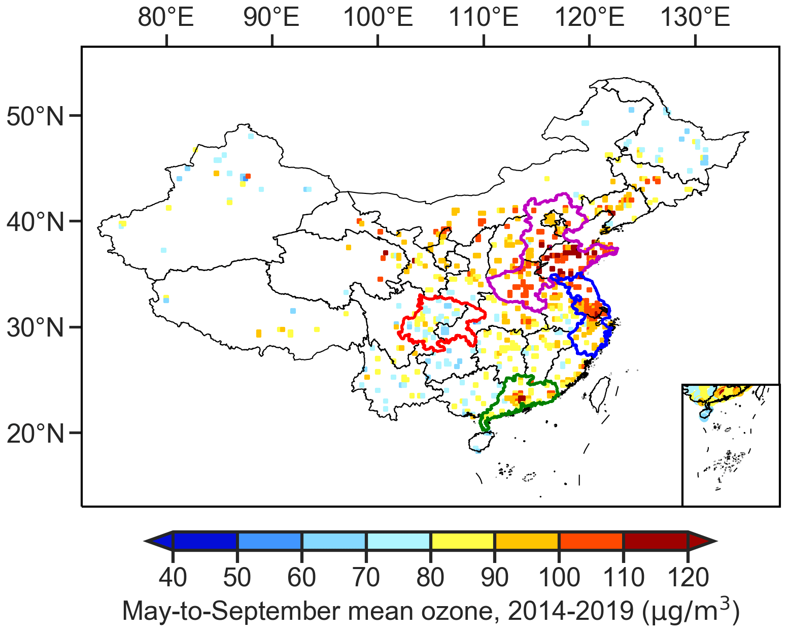
Figure 1The May-to-September mean hourly surface ozone network data from 2014 to 2019. Mean hourly surface ozone concentrations are calculated on the grid. Purple, blue, green, and red outlines indicate the boundaries of North China Plain (NCP), Yangtze River Delta (YRD), Pearl River Delta (PRD), and Sichuan Basin (SCB), respectively.
2.1 Data sources
In this study, Ozone Monitoring Instrument (OMI) datasets were employed for exploring the spatiotemporal variations in HCHO and NO2 in China and calculating . We connected surface ozone network data to HCHO, NO2, and , which served as the input data for running third-polynomial model and convergent cross-mapping (CCM). The MODIS land cover product provided the spatial distribution of urban areas, which was employed for identifying urban and rural pixels.
2.1.1 OMI
The Ozone Monitoring Instrument (OMI), on board the Aura satellite, monitors global solar backscatter in the UV–vis domain (270–500 nm). The OMI provides daily global observations and crosses the Equator at 13:38 LT (Levelt et al., 2006). In this study, we employed the daily level-3 gridded OMI HCHO product (OMHCHOd) from the Smith Astrophysical Observatory (SAO) (González Abad et al., 2015). The HCHO vertical columns are the weighted mean values for the grid. Backscattered solar radiation, ranging from 328.5–356.5 nm, was used for fitting HCHO slant columns. Air mass factors (AMFs) were employed for converting HCHO slant columns to vertical columns (González Abad et al., 2015). The validation report suggested that the error in this product was effectively controlled within 30 % over polluted areas (González Abad et al., 2015) and validated for detecting long-term variations in HCHO columns (Zhu et al., 2017; Shen et al., 2019b). The daily level-3 gridded OMI NO2 product (OMNO2d), provided by NASA's Goddard Space Flight Center, was utilized in this study (Bucsela et al., 2013; Lamsal et al., 2014). The spatial resolution of OMNO2d is 0.25∘, and each grid is generated as the weighted average of the corresponding level-2 data pixels (Krotkov et al., 2017). Differential optical absorption spectroscopy (DOAS) was employed for retrieving the NO2 slant columns, which were successively transformed into tropospheric and stratospheric vertical columns through AMFs (Bucsela et al., 2013). The OMI NO2 column product agrees well with other satellite products, and its overall uncertainties range from 30 %–60 % (Bucsela et al., 2013; Lamsal et al., 2014). To reduce uncertainties, we only selected those OMI HCHO and NO2 data that (1) passed quality checks, (2) had a cloud coverage less than 30 %, (3) had a solar zenith angle less than 60∘, and (4) were not affected by row anomalies for this study (Kroon et al., 2011; Zhu et al., 2014; Krotkov et al., 2017). The May-to-September OMI HCHO and NO2 products were acquired from NASA's Goddard Earth Sciences Data and Information Services Center (https://disc.gsfc.nasa.gov/, last access: 1 September 2021).
2.1.2 Surface ozone network data
The May-to-September hourly surface ozone concentrations from 2014 to 2019 were obtained from the China Ministry of Ecology and Environment (MEE) (https://quotsoft.net/air/, last access: 1 September 2021). The unit of surface ozone concentrations in this dataset is µg m−3. The network had 1633 monitoring stations, which were distributed among 330 cities across China in 2019. We used the observation data from 13:00 to 14:00 LT to match the overpass time of the OMI. This dataset has been employed in many studies to investigate the variations in surface ozone concentrations in China (Li et al., 2019a; Shen et al., 2019a; Lu et al., 2020).
2.1.3 MODIS land cover product
The annual MODIS land cover product (MCD12C1) with a spatial resolution of 0.05∘ from 2005 to 2019 was employed for extracting urban and rural areas. The urban and water pixels from the International Geosphere–Biosphere Program (IGBP) classification layer were employed for the following processing. The land cover product was generated based on a decision tree algorithm with boosting techniques, and its overall accuracy was about 75 % (Palmer et al., 2015; Bajocco et al., 2018). The MCD12C1 product was obtained from NASA's Earth System Data and Information System (https://earthdata.nasa.gov/, last access: 1 September 2021).
2.1.4 Data pre-processing
Due to the different spatial resolution of OMI HCHO, OMI NO2, and MCD12C1, a bilinear interpolation method was used for resampling all abovementioned products to the same spatial size (). Meanwhile, we also calculated mean hourly surface ozone concentrations on the grid (Fig. 1).
2.2 Methods
Chemical transport models, such as the global chemical transport model (GEOS-Chem) (Jin et al., 2017; Li et al., 2019a) and the Community Multiscale Air Quality Modeling System (CMAQ) (Duncan et al., 2010), have been frequently employed for exploring the ozone sensitivity to VOCs and NOx. However, there were large biases in estimating the range of the transitional regime based on chemical transport models (Jin et al., 2017, 2020) due to the uncertainties in the emission inventory and the setting of model parameters. Employing observation data alone could effectively overcome these limitations, and the relationships between ozone and its precursors were fitted using linear and polynomial models (Sun et al., 2018; Jin et al., 2020). Meanwhile, convergent cross-mapping (CCM) (Sugihara et al., 2012), as a robust causality analysis model, has been widely employed for quantifying the influences of meteorological factors on surface ozone and PM2.5 concentrations (Chen et al., 2018, 2019c, 2020). It is a promising tool for investigating the relationships between ozone and its precursors. To increase the reliability of the estimated range of the transitional regime, both the polynomial model and CCM were employed in this research. We employed the third-order polynomial model for fitting surface ozone concentrations to the indicator of . CCM was employed for quantifying the influences of HCHO and NO2 on surface ozone concentrations, and the Wilcoxon test (Gehan, 1965) was used for examining whether the differences between the causality of HCHO on ozone and NO2 on ozone at different ranges of was significant. Since the algorithms of the two models are quite different, their cross-verification provides useful reference for their reliability. Meanwhile, the Mann–Kendall (M–K) test (Kendall, 1970) was employed for exploring the spatiotemporal variations in HCHO, NO2, and ozone formation regimes in China. Furthermore, we extracted all urban and rural areas in China and compared the differences in ozone formation regimes over these two types of areas. The workflow of the models employed in this study is shown in Fig. 2.

2.2.1 Estimating the transitional range of the ozone formation regime using polynomial simulation
HCHO and NO2 are considered to be proxies for VOCs and NOx, respectively. , as an effective indicator, has been widely employed for determining ozone formation regimes (Duncan et al., 2010; Jin and Holloway, 2015; Jin et al., 2017, 2020; Cheng et al., 2019). Pusede and Cohen (2012) suggested that ozone exceedance probability (OEP) was an effective indicator to interpret the ozone sensitivity to its precursors. The indicator is defined as the proportion of non-attainment events (surface ozone concentrations exceeding 200 µg m−3) in total events at a given range of :
where Eventsattainment and Eventsnon-attainment denote the attainment and non-attainment events, respectively (Pusede and Cohen, 2012; Jin et al., 2020).
In this study, we used a third-order polynomial model (Jin et al., 2020) to explore the quantitative relationships between and ozone exceedance probability. There were 174 868 paired observations of surface ozone concentrations and from 2014 to 2019. The peak of fitting curve highlights the turning point of VOC-limited and NOx-limited regimes (Jin et al., 2020). The range of , which corresponded to the top 10 % ozone exceedance probability, was defined as the transitional regime. Since we aimed to apply a global model to determine the transitional range, it was necessary to examine whether the surface ozone concentrations in China were of spatially stratified heterogeneity (SSH), as suggested by Wang et al. (2016). We employed the geographical detector (Wang et al., 2010) to measure the SSH of surface ozone concentrations. The geographical detector calculates the q statistic to quantify SSH, and the equation is summarized as follows:
where N and σ2 denote the number of samples and the variance of population, and h is the number of stratifications. The range of the q statistic is [0, 1]. The larger the q statistic is, the stronger the SSH is. In this study, the boundaries of four megacity clusters served as strata. If the SSH is detected based on the abovementioned stratification, we could apply the polynomial model in each strata separately.
2.2.2 Estimating the transitional range of the ozone formation regime using convergent cross-mapping
We also employed a causality model named convergent cross-mapping (CCM) (Sugihara et al., 2012), which could reduce the influences of other factors such as meteorological conditions (Chen et al., 2019c, 2020), to extract the causal influences of HCHO and NO2 on surface ozone concentrations. Thanks to its capability of detecting weak coupling, CCM is advantageous for reliably comparing the influences of different meteorological factors on surface ozone concentrations (Chen et al., 2020). Therefore, we employed CCM to compare the sensitivity of ozone to HCHO and NO2 at different ranges of . CCM utilizes convergent maps to demonstrate the bidirectional coupling between the time series of two variables. A convergent curve indicates that one variable imposes influences on the other variable, whilst a non-convergent curve denotes no causality between two variables. The main idea of CCM is summarized as follows. Firstly, CCM defines {X} and {Y} as the temporal variations in two variables X and Y. {X} generates the shadow manifold MX. Following this, the location of the lagged-coordinate vector on MX, x(t) is determined, and then E+1 nearest neighboring points of x(t) are extracted. Finally, the cross-mapped estimate of Y(t), Y(t)|MX is calculated as follows:
where ωi stands for a weight calculated based on the distance between X(t) and its ith nearest neighboring point. Y(ti) stands for the contemporaneous value of Y. CCM calculates cross-map skill (ρ value), which explains the quantitative relationships. Number of dimensions for the attractor reconstruction (E), time lag (τ), and number of nearest neighbors to use for prediction (b) are required parameters for CCM. According to previous studies (Chen et al., 2019c, 2020), E, τ, and b were set as 3, 2, and 4, respectively. Since the existence of missing values imposes negative impacts on CCM results, only the consecutive time series were retained for this research. There were 1660 observation records of HCHO time series, NO2 time series, and corresponding surface ozone time series. CCM was implemented using the “pyEDM” package in Python. The Wilcoxon test (Gehan, 1965) was used to examine whether the differences in ρ values between HCHO and NO2 were significant at the given . No significant difference was regarded as the transitional regime, while significant difference indicated the VOC-limited or NOx-limited regime.
2.2.3 Trend analysis
The Mann–Kendall (M–K) (Kendall, 1970) test, which has been used in recent studies on HCHO and NO2 (Cheng et al., 2019; Wang et al., 2019; Zeb et al., 2019), was employed to estimate the significance of trends. The M–K test is capable of processing samples with random distributions and mitigating the effects of outliers. The Z value is calculated as follows:
where S denotes the statistic to be tested, and Var(S) stands for the variance of S. The sign and absolute value of Z indicate the direction and significance of trends, respectively. Specifically, the positive and negative values of Z indicate the upward and downward trend; 1.28, 1.64, and 2.32 are the threshold values of , indicating that the trends of samples pass the tests at 90 %, 95 %, and 99 %, respectively.
2.2.4 Comparison of ozone formation regimes in urban and rural areas in China
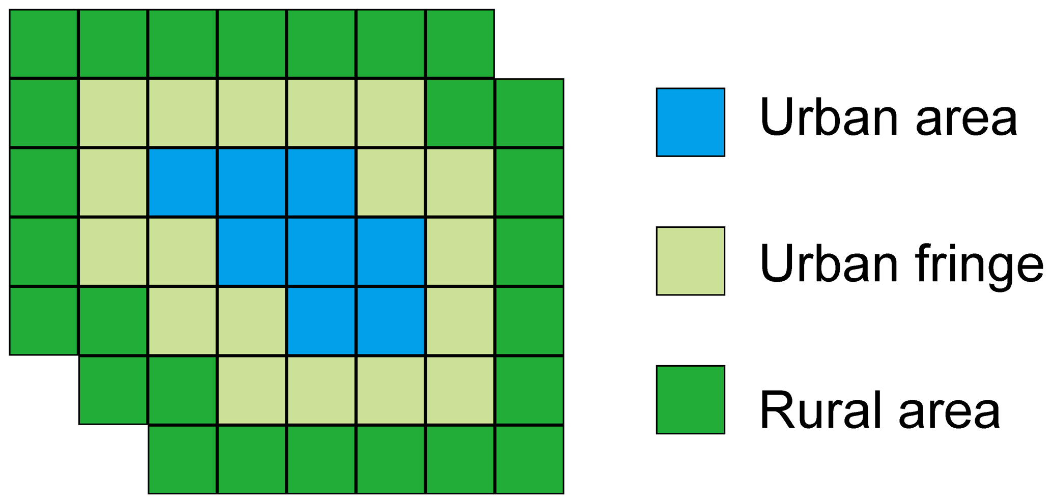
To compare the differences in ozone formation regimes in urban and rural areas in China, the key step is to extract urban and rural pixels, respectively. Urban pixels were used for buffer analysis (Imhoff et al., 2010) to identify rural pixels. Following Peng et al. (2018), two buffers were set for urban pixels to extract candidate rural pixels (Fig. 3). We set the size of each buffer as 27.75 km, which was close to the size of the grid (). The first and second buffers were determined as the urban fringes and candidate rural areas, respectively. Water pixels were firstly removed from candidate rural areas to avoid following uncertainties. Consequently, rural areas were regarded as buffers of 27.75–55.50 km surrounding urban areas. The use of two buffers not only assisted a complete separation of the urban and rural areas but also minimized the uncertainties in meteorological conditions (Yao et al., 2019).
3.1 Spatial and temporal variations in HCHO and NO2
Given the national Clean Air Action implemented in 2013, we set this year as a break point to explore the spatial and temporal variations in HCHO and NO2 in 2005–2012 and 2013–2019, respectively. Figure 4 shows the spatial distribution of HCHO in the two periods. The mean HCHO values during the period of 2005–2012 and 2013–2019 were 4.335×10¹⁵ and 4.845×10¹⁵ , characterized by a 12 % increase. Both periods presented an increasing trend of HCHO, and the averaged values during the two periods were 0.164×10¹⁵ and 0.213×10¹⁵ (Fig. 5). A faster increasing trend was detected during the period of 2013–2019. The variation trend of HCHO agreed well with previous studies (Jin and Holloway, 2015; Shen et al., 2019b). We also calculated the overall linear trends of HCHO in four megacity clusters from 2005 to 2019 (Fig. 6). The largest and smallest increasing trends were shown in the NCP and SCB, with a mean value of 0.136×10¹⁵ and 0.046×10¹⁵ . The increasing trends of the YRD and PRD were 0.066 and 0.058 , respectively. Meanwhile, reversed trends were detected for NO2 during the two periods (Fig. 5), which was consistent with previous studies (Jin and Holloway, 2015; Li et al., 2019a). From 2005 to 2012, the averaged NO2 was 2.027×10¹⁵ , and the annual mean increasing trend was 0.098×10¹⁵ . Thanks to the implementation of the Clean Air Action, the averaged NO2 was reduced to 1.900×10¹⁵ , with a decreasing trend of from 2013 to 2019. Except for the SCB, all other megacity clusters presented significant downward trends of NO2 from 2005 to 2019. Amongst these megacity clusters, NO2 in the YRD demonstrated the largest decreasing trend of 0.104×10¹⁵ . NO2 in the NCP and PRD decreased by 0.010×10¹⁵ and 0.092×10¹⁵ , respectively. A slightly increasing trend of 0.012×10¹⁵ was detected in the SCB (Fig. 7).
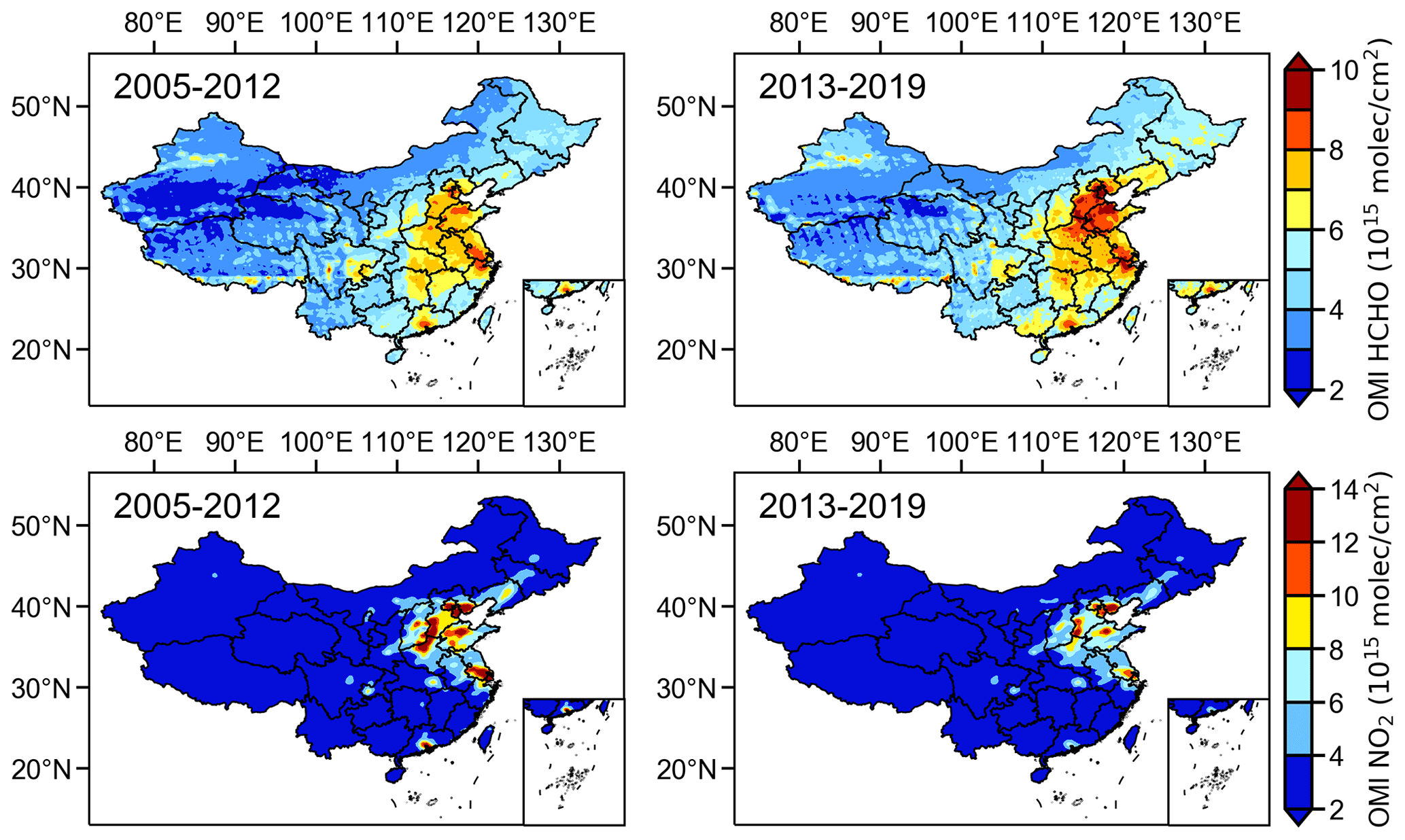
Figure 4May-to-September averaged HCHO and NO2 across China during the period of 2005–2012 and 2013–2019.
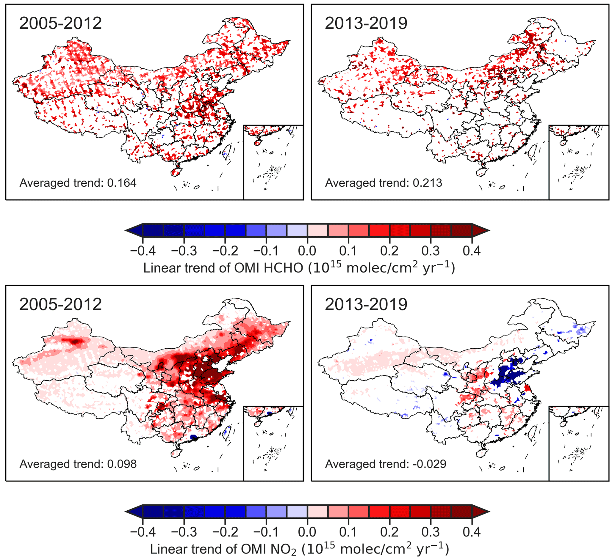
Figure 5The linear trends of May-to-September HCHO and NO2 across China during the period of 2005–2012 and 2013–2019.
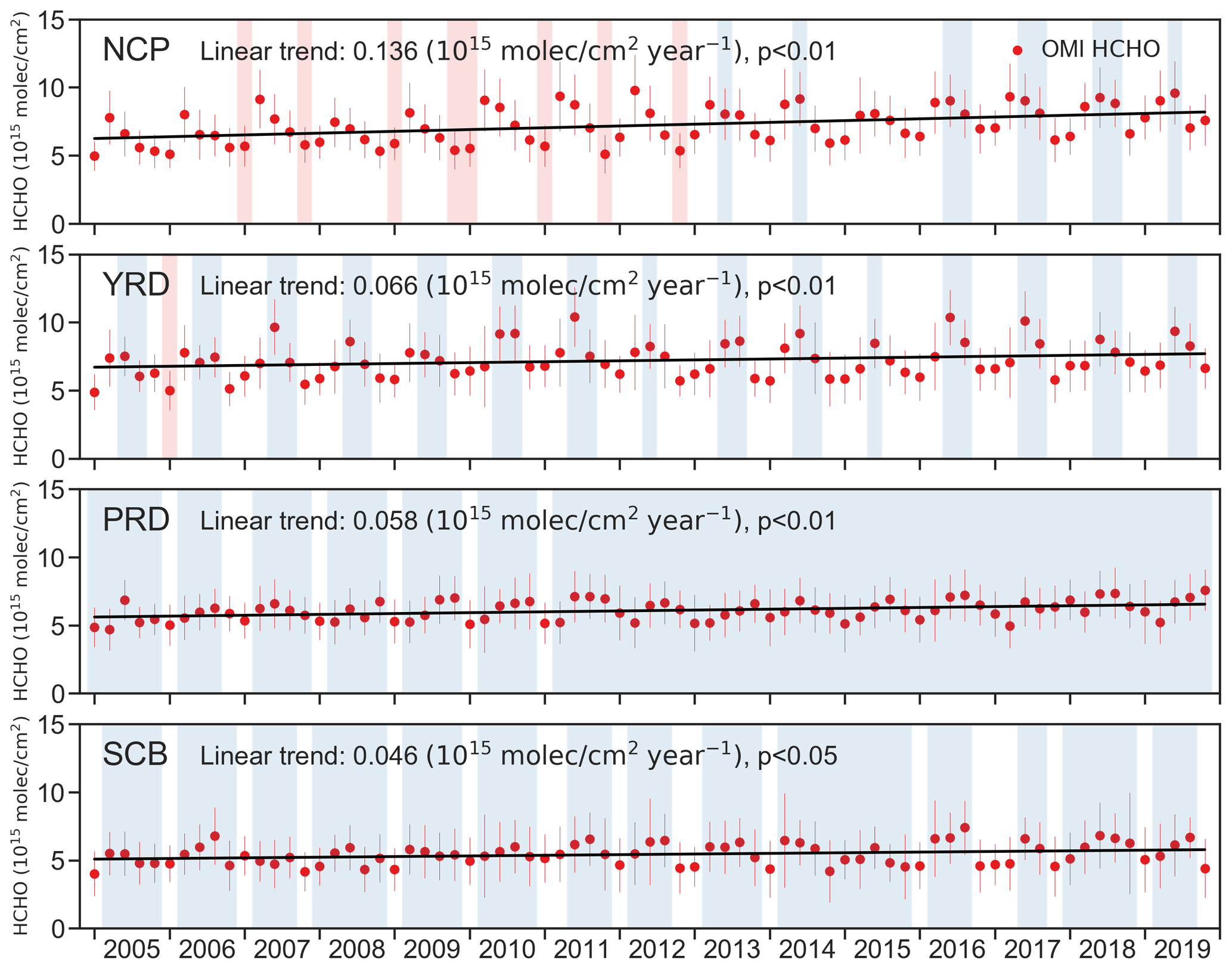
Figure 6The time series of HCHO columns in the four megacity clusters from 2005 to 2019. Black lines indicate the linear trend of HCHO columns. Red, white, and blue areas stand for VOC-limited, transitional, and NOx-limited regimes, respectively.
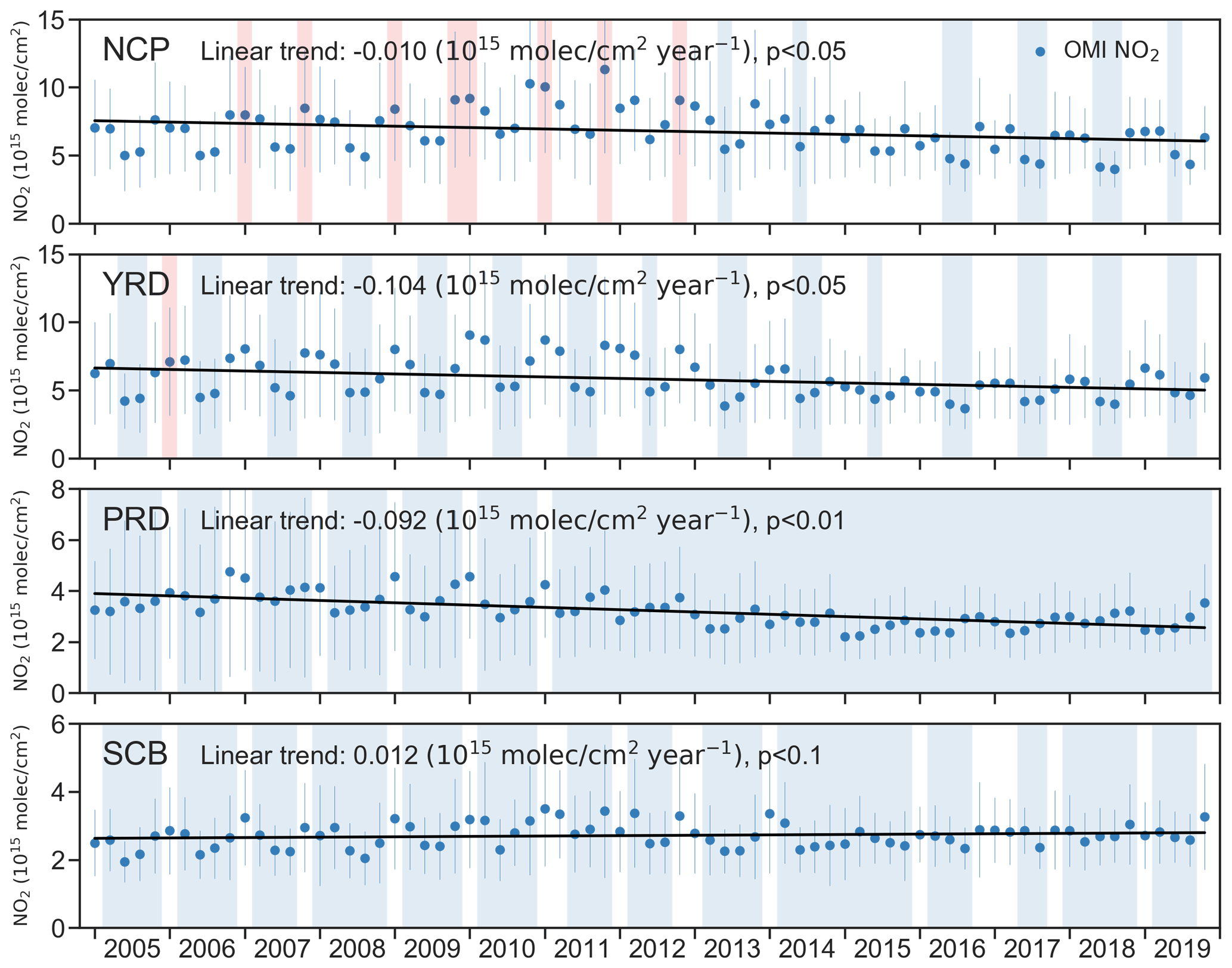
Figure 7The time series of NO2 columns in the four megacity clusters from 2005 to 2019. Black lines indicate the linear trend of NO2 columns. Red, white, and blue areas stand for VOC-limited, transitional, and NOx-limited regimes, respectively.
3.2 Transitional range of the ozone formation regime
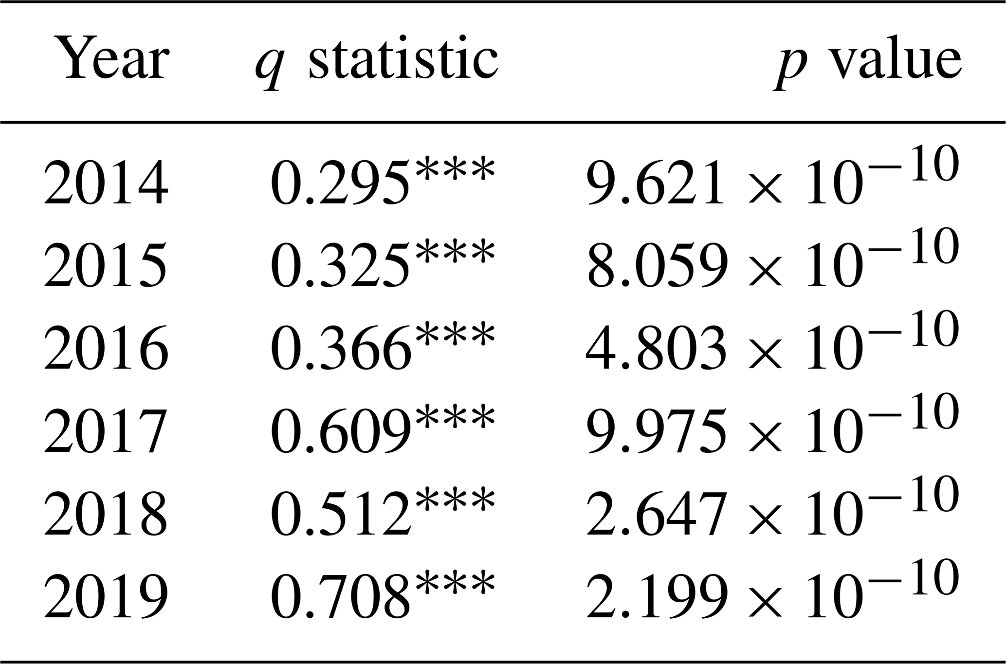
According to , we divided the paired observations into 200 bins for the whole country, and the ozone exceedance probability was calculated for each bin. The third-order polynomial was employed for fitting ozone exceedance probability to . As shown in Fig. 8a, the peak of the fitting curve was 1.4, and the vertical shaded area indicated that the transitional regime over China ranged from 1.0 to 1.9. We employed a geographical detector to examine the SSH of annual May-to-September mean surface ozone concentrations in China. As shown in Table 1, all the q statistics from 2014 to 2019 were greater than zero, which indicated that the surface ozone concentrations in China were of SSH. As suggested by Chen et al. (2020), meteorological factors including temperature, humidity, and sunshine duration imposed great impacts on surface ozone concentration. Moreover, the composition of ozone precursors was closely related to ozone levels (Cheng et al., 2019). Both the meteorological conditions and ozone precursors contributed to the SSH of surface ozone concentrations across China. Therefore, in addition to the regime range extracted at the national scale, we also examined the range of ozone formation regimes in four major megacity clusters. The paired observations of these megacity clusters were divided into 100 bins. The range of the transitional regime for the NCP, YRD, PRD, and SCB was [1.2, 2.1], [1.0, 1.9], [0.9, 1.8], and [1.1, 2.0], respectively, which was generally consistent with the range at the national scale. The small differences between four megacity clusters across China suggested that the range of the transitional regime at the national scale [1.0, 1.9] can be employed to regional- or local-scale research if small-scale data and investigation were not available.
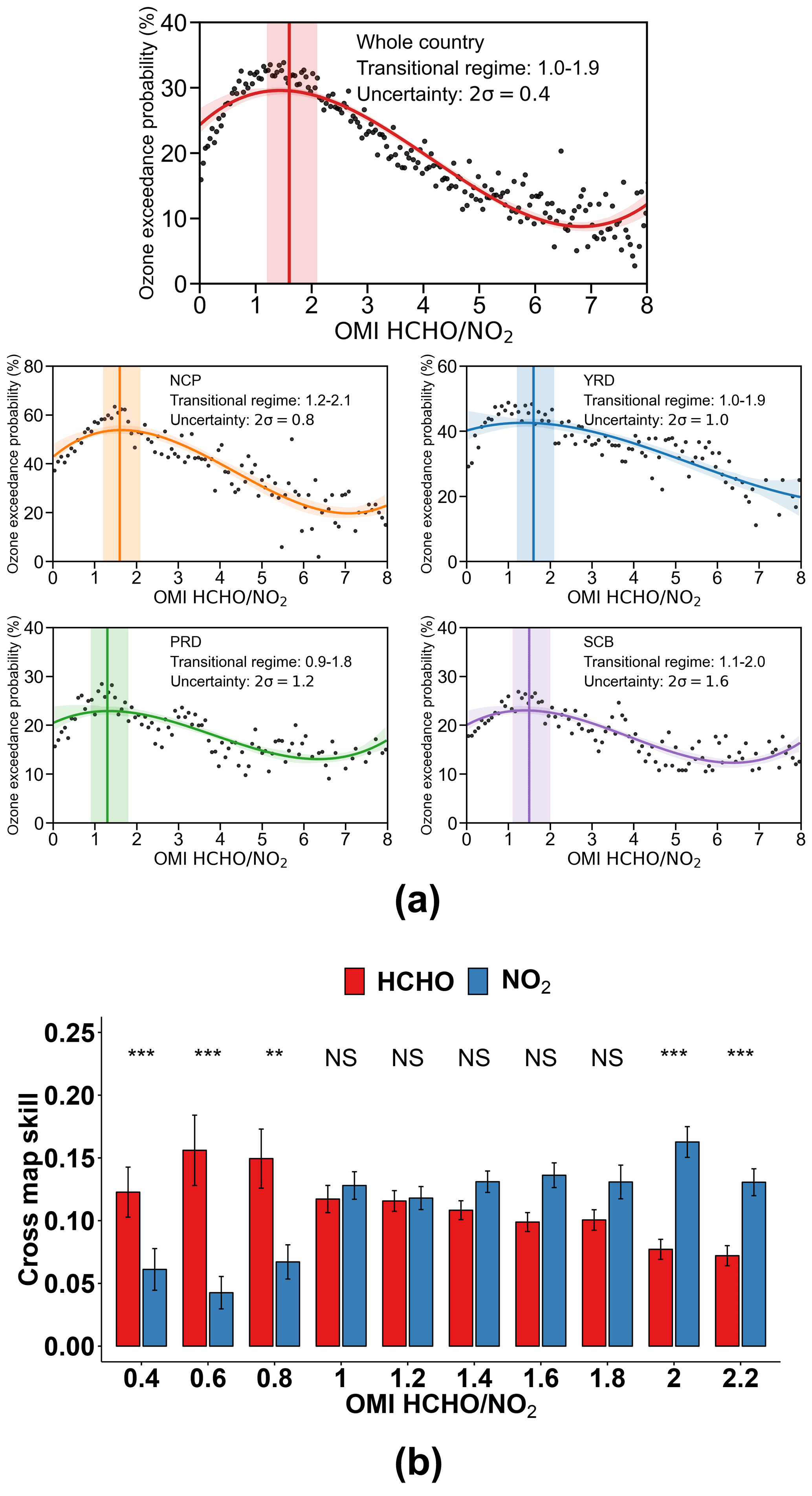
Figure 8(a) Fitting ozone exceedance probability to through the third-order polynomial model. The curve indicates the fitting result of the third-order polynomial. The vertical line denotes the maximum of the curve, and the shaded area represents the top 10 % ozone exceedance probability. (b) The cross-map skill of HCHO and NO2 on surface ozone (the skill of using HCHO and NO2 for predicting surface ozone concentrations) at different ranges of . The symbols and texts above the bars are the results of the Wilcoxon test. and indicate that the difference was significant at the p=0.01 and 0.05 confidence level, respectively. NS suggests non-significant differences.
Table 1The q statistic and p value calculated by the geographical detector, which indicate the SSH of annual May-to-September mean surface ozone concentrations in China. *, , and of the p value indicate statistical significance at the α=0.05*, 0.01, and <0.001 level, respectively.
Statistical bootstrapping was used for estimating the uncertainty in the fitting model. Specifically, we iteratively extracted 50 randomly selected subsets from the paired observations to run the model, and the uncertainty was defined as 2 standard deviations from the peak of the fitting curve. The uncertainty for the third-polynomial model was 0.4, indicating a significant nonlinear relationship between ozone exceedance probability and .
Due to the limited data used for running CCM, we set the bin size of as 0.2 for collecting sufficient ρ values to conduct the Wilcoxon test. As shown in Fig. 8b, there was no significant difference between ρ of HCHO and NO2 when ranged from 0.9 to 1.9, which indirectly defined the range of the transitional regime. For , ρ of HCHO was notably higher than that of NO2, and this range was regarded as the VOC-limited regime. Similarly, suggested the NOx-limited regime. Through the cross-verification, it was an important finding that the range of the transitional ozone formation regime estimated using the third-order polynomial model and CCM was highly close, indicating the reliability of the extracted range.
3.3 Ozone formation regimes in China
NO2 demonstrated a significant downward trend since 2013, while HCHO kept the increasing trend during the entire study period. Consequently, increased in a majority of regions across China. Specifically, the annually increasing trend of in the NCP, YRD, and PRD was 0.035, 0.023, and 0.034 yr−1, respectively. Meanwhile, there were no significant trends in the SCB during this period (Fig. 9). The variations in indicated the shrinkage of the VOC-limited regime and the expansion of the transitional and NOx-limited regimes. Since the range of the transitional regime estimated by the third-order polynomial model and CCM was very close, and the former included more reliable observation data, [1.0, 1.9] was employed for identifying different ozone formation regimes. In 2005, areas with the VOC-limited regime were concentrated in the NCP, YRD, and PRD. The proportions of areas with the VOC-limited regime in the NCP, YRD, and PRD were 26 %, 16 %, and 6 %, respectively. Areas with the transitional regime were mainly distributed in the marginal regions of those megacity clusters and scatteredly distributed in the SCB. Areas with the transitional regime occupied 60 %, 50 %, 14 %, and 20 % in the NCP, YRD, PRD, and SCB. The NOx-limited regime dominated other areas (Fig. 10a). In 2019, areas with the VOC-limited regime decreased significantly; this regime was simply found in the fringe areas of the NCP and YRD. The proportion of the VOC-limited regime in the NCP and YRD was 2 % and 9 %, respectively. The transitional regime was widely distributed throughout the NCP, YRD, and SCB and occupied 71 %, 56 %, and 36 % of the total areas. The NOx-limited regime still spread over a majority of China (Fig. 10a). We calculated the annual mean ρ of HCHO and NO2 over those megacity clusters from 2014 to 2019 (Fig. 10b). For all megacity clusters, the ρ of NO2 was higher than HCHO, indicating that NO2 was the dominant factor for surface ozone concentrations. Both models suggested that NO2 played a more important role in affecting surface ozone concentrations than HCHO. In the past several years, NOx-oriented emission reduction has been conducted across China, leading to the continuous decrease in NOx concentrations. Since both VOCs and NOx imposed positive influences on surface ozone concentrations under the transitional and NOx-limited ozone formation regime, the upward trend of HCHO across China might explain recent soaring ozone concentrations across China (Shen et al., 2019a; Lu et al., 2020). It is noted that the difference between the ρ of NO2 and HCHO decreased notably in the NCP and YRD. This may be attributed to the following reason. The NCP and YRD are the regions that received severe PM2.5 pollution, and strict NOx reduction policies have been conducted since 2013. With the remarkably reduced NO2 concentrations, the variations in HCHO concentrations plays an increasingly important role in affecting ozone concentrations in the NCP and YRD. The reduction in VOC emissions is key for an effective management of surface ozone pollution in the NCP and YRD.
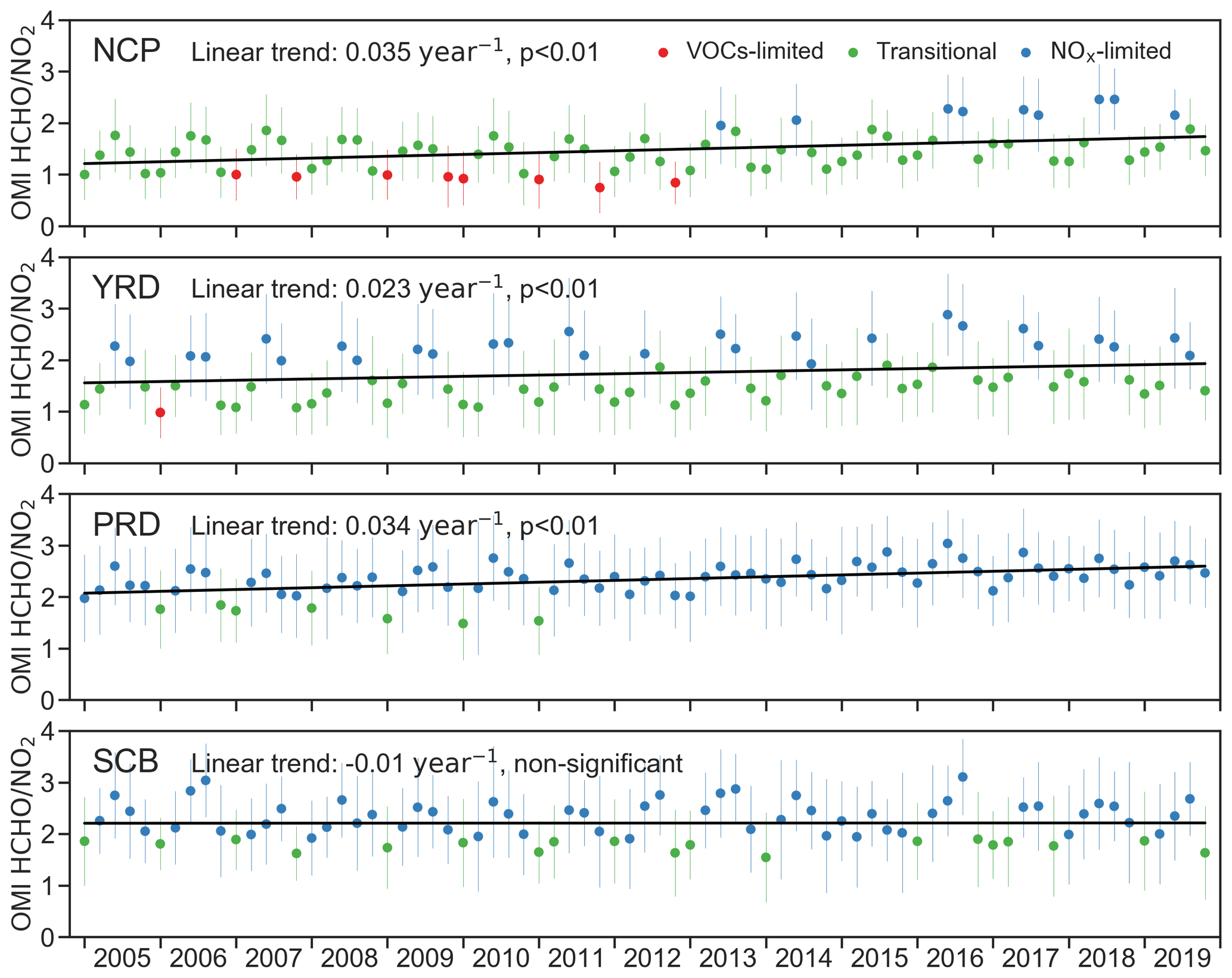
Figure 9The time series of in the four megacity clusters from 2005 to 2019. Black lines indicate the linear trend of . Red, green, and blue dots stand for VOC-limited, transitional, and NOx-limited regimes, respectively.

Figure 10(a) The spatial distribution of across China in 2005 and 2019. The boundaries of the NCP, YRD, PRD, and SCB are denoted with the purple, blue, yellow, and red bold lines. Red, green, and blue stand for VOC-limited, transitional, and NOx-limited regimes. (b) The annual mean cross-map skill (ρ value) of four megacity clusters. The red and blue shadow areas indicate the standard deviations.
3.4 Variations in ozone formation regimes in urban and rural areas
Previous studies suggested that the differences in ozone formation regimes existed between urban and rural areas (Tong et al., 2017; Y. Liu et al., 2018; Cheng et al., 2019). We extracted HCHO and NO2 columns in urban and rural pixels in those megacity clusters and calculated the annually averaged (Fig. 11). For the NCP, in urban areas was higher than 1.0 since 2015, indicating a transformation from the VOC-limited to the transitional regime. The increase in was attributed to the reversed variation trends of HCHO and NO2. The rising HCHO resulted from the increase in anthropogenic emissions and biogenic volatile organic compounds (BVOCs) (Shen et al., 2019b; Wang et al., 2020), while the implementation of the Clean Air Action imposed notable influences on the decrease in NO2 (Chen et al., 2019a). in rural areas was in the range of [1.0, 1.9], indicating that rural areas were occupied by the transitional regime from 2005 to 2019. For the YRD, which was occupied by the transitional regime, no variation in ozone formation regime was found in urban areas. In rural areas, temporally exceeded the threshold of 1.9 from 2016 to 2018, indicating that the ozone formation regime changed from transitional to NOx-limited. This phenomenon was attributed to the slight decline in HCHO, which might be attributed to the restrictions on crop residue burning in this area (Zhuang et al., 2018; Shen et al., 2019b). Due to the large differences in NO2 concentrations, the urban and rural areas in the PRD were dominated by the transitional regime and NOx-limited regime. For the SCB, in both urban and rural areas fluctuated around the threshold value of 1.9, and no significant difference between urban and rural areas was found.
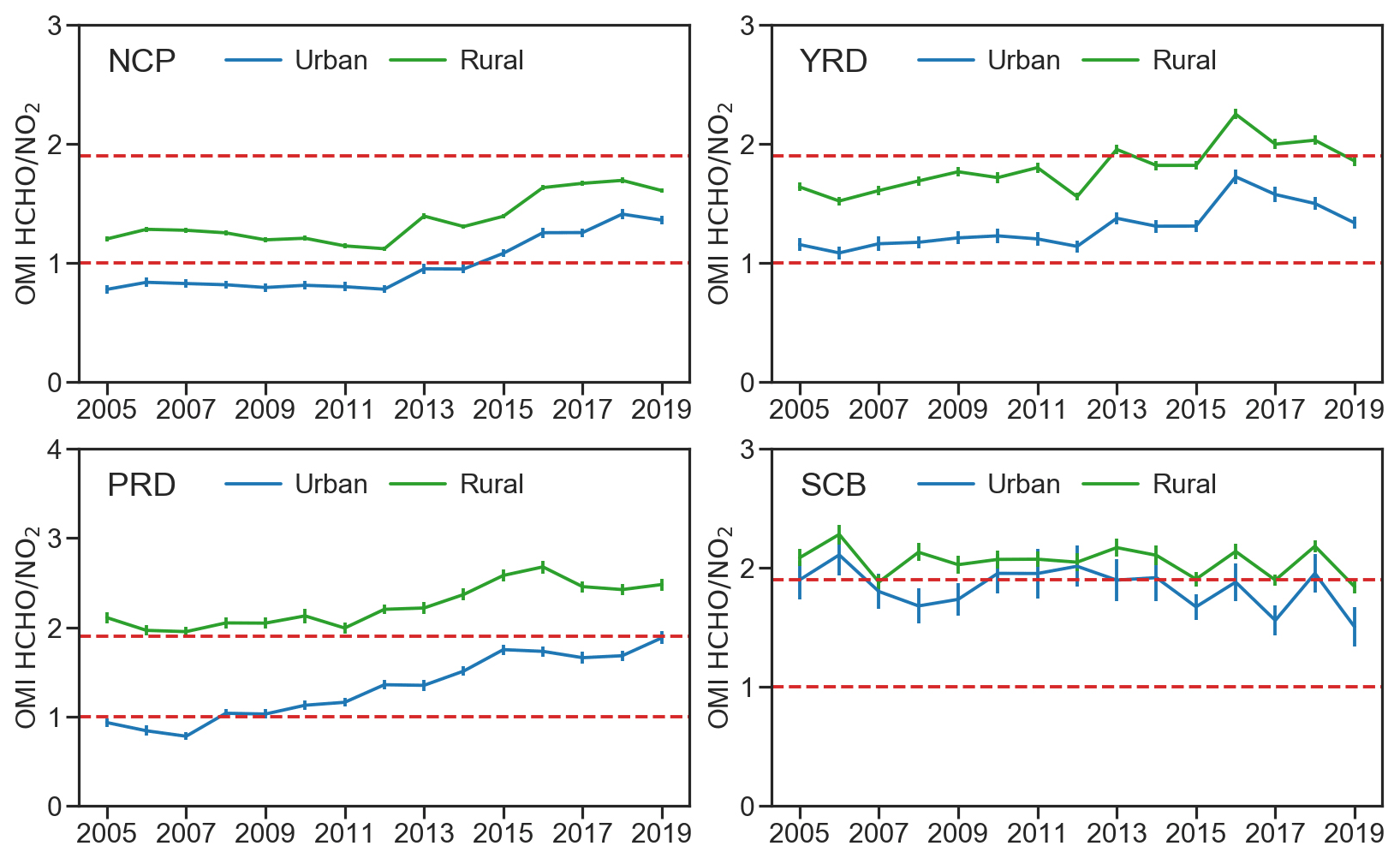
Figure 11The temporal variations in from 2005 to 2019 in the NCP, YRD, PRD, and SCB. The two dashed red lines indicate the threshold values of 1.0 and 1.9, which separate the NOx-limited, transitional, and VOC-limited regime.
This research employed CCM and a third-order polynomial model to estimate the transitional regime of ozone formation across China, and the calculated range of was [0.9, 1.9] and [1.0, 1.9], respectively. Our findings were generally consistent with previous studies. For the US, Duncan et al. (2010) and Choi et al. (2012) employed the OMI and GOME-2 data, whose 0.25∘ resolution was close to this research, and calculated the range of the transitional regime as [1.0, 2.0]. The similar range of the transitional regime in the US and China further proved the reliability of the calculated range [1.0, 1.9] at a national scale. On the other hand, the range of the transitional regime can vary significantly across regions (Schroeder et al., 2017; Jin et al., 2020). Sun et al. (2018) employed station-based data and calculated the range of the transitional regime in Anhui Province, China, as [1.3, 2.8], which was notably higher than the range across China. Jin et al. (2020) calculated the range of the transitional regime in several major regions in the US using the QA4ECV dataset, whose spatial resolution was 0.125∘, and the output [3.2, 4.1] was much larger than the averaged range of the transitional regime across the US. One reason could be the severe ozone pollution in megacities, leading to different ranges of the transitional regime. Meanwhile, the calculated range of the transitional regime is closely related to the spatial resolution of employed HCHO and NO2 data, and high-resolution data are more advantageous in extracting the sensitivity of ozone concentrations to precursors at the local scale (Martin et al., 2004; Jin et al., 2017, 2020). In addition to the generally consistent outputs, some advances of this research are listed as follows. First, only a few parameters are required for the polynomial model and CCM, which effectively reduced the uncertainties in model setting. Second, considering the differences between model and satellite-retrieved datasets (Jin et al., 2020), only observation data were employed in this research, which reduced potential data inconsistences and uncertainties. Most importantly, given the lack of actual reference data, this research employed two different models to examine ozone formation regimes, and the close outputs further proved the reliability of this research.
Despite a generally reliable output, some uncertainties exist. First, the accuracy of the estimated range of the transitional regime might be influenced by the scaling biases between station-based observations of surface ozone and space-based HCHO and NO2. Since ozone monitoring stations are mainly distributed in urban areas, and a grid might cover both the urban and rural areas, the surface ozone concentrations of a grid may be overestimated. Second, the uncertainties in OMI HCHO and NO2 datasets might impose negative influences on the estimation of the transitional regime range (Duncan et al., 2010; Jin et al., 2017, 2020; Schroeder et al., 2017). On one hand, errors exist in the retrieval of HCHO and NO2 vertical columns. On the other hand, vertical mixing was not homogeneous, weakening the capability of using HCHO and NO2 vertical columns to explore the near-surface ozone–precursor sensitivity. Therefore, future improvement of earth observation techniques and the spatiotemporal resolution of HCHO and NO2 products can further enhance the accuracy of the estimated range of the transitional regime. In general, according to the cross-verification and comparison with previous studies, [1.0, 1.9] from this research is a reliable range for the transitional ozone formation regime across China and can be used as an approximate criterion to follow when implementing national emission reduction policies. On the other hand, given the potential variations in transitional regimes in different regions, when conducting small-scale research, the range of [1.0, 1.9] may be adapted accordingly based on local data.
Previous studies on the range of ozone formation regimes were mainly conducted using statistical models or chemical transport models. For this research, we employed both a statistical and a causality model to cross-verify the range of the transitional regimes. Despite a relatively high fitting accuracy in terms of uncertainties, the findings from these studies could not be effectively compared or interpreted due to the lack of reliable reference data. To this end, as well as numerical models, lab experiments should also be considered to extract a more precise description of the ozone–precursor relationship. With the rapid development of atmospheric science, smog chambers have been increasingly employed to investigate complicated interactions between multiple precursors. By setting specific meteorological conditions (e.g., temperature and humidity) and gradually adjusting the proportion of different precursors, how the proportion of NO2 and HCHO affects the ozone formation regime can be better explained in a theoretical environment. With more reliable experimental reference data, the model-based analysis on the range of the transitional regime at the local, regional, and national scale can be further improved accordingly.
According to the temporal variations in OMI NO2 concentrations across China, a notable decreasing trend was observed in three major megacity clusters: NCP, YRD, and PRD. These regions were heavily polluted by PM2.5, and the notable decrease in NO2 was mainly attributed to the national Clean Air Action since 2013 (Zheng et al., 2018), which aimed to reduce PM2.5 concentrations by cutting NOx emissions. The influence of the Clean Air Action on the reduction in PM2.5 concentrations and NOx has been investigated by previous studies. Zheng et al. (2018) employed index decomposition analysis to quantify the contribution of the Clean Air Action and suggested that the decreasing rate of NOx significantly accelerated since 2013. Moreover, Y. Zhang et al. (2020) employed a random forest algorithm to remove the effects of meteorological conditions and evaluated the impacts of the Clean Air Action. The results demonstrated that the deweathered NO2 concentrations in winter 2007 and 2017 were 70.3 and 59.1 µg m−3, with a decreasing rate of 16 %. Conversely, HCHO concentrations during this period increased remarkably across China due to the combined effects of anthropogenic and biogenetic emissions (Shen et al., 2019b; Wang et al., 2020). The distinct temporal variations in NO2 and HCHO led to the increase in and the increase in transitional areas and NOx-limited regime areas. From 2013–2019, all these regions were dominated by the transitional or NOx-limited regimes. Attributed to the long-term variation in formation regimes, a more complicated and fragmented spatial pattern was observed across China. Consequently, for an effective control of ozone pollution, the emission reduction in both NOx and VOCs is required. Especially for the NCP and YRD, where the NOx has been remarkably reduced, effective approaches for controlling VOC emissions are essential for preventing ozone pollution. This finding was consistent with previous studies (Li et al., 2019b), which recommended the simultaneous reduction in NOx and VOCs for mitigating the composite airborne pollution in China. Admittedly, compared with NOx reduction, the VOC reduction is more complicated, and the output of anthropogenic VOC reduction is more unpredictable. In this case, reducing biogenic VOC emissions can also be a potential solution. VOCs emitted by vegetation take up to 50 % of total VOCs in the atmospheric environment, especially in summer. The key factor that may cause enhanced biogenic emissions is summertime high temperature (Chen et al., 2020). Therefore, such projects as wind corridors or contingent artificial precipitation, which can effectively reduce urban heat effects, should be implemented properly to avoid summertime heat waves and successive ozone pollution (e.g., summer, 2017).
The large spatial variations in , especially the rapid increase in transitional regime areas across China, indicate that a unified NOx–VOC reduction strategy is not feasible for the entire country. Instead, to effectively reduce ozone concentrations, the specific proportion of NOx and VOC reduction should be carefully set according to local . Meanwhile, due to the large differences in vehicle and industrial emissions (Cheng et al., 2019), the concentration of NOx is notably higher in urban areas. Therefore, the further reduction in NOx emissions exerts a stronger influence on ozone reduction in rural areas compared to urban areas.
To better understand the spatiotemporal variations in ozone formation regimes across China, we employed the third-order polynomial model and CCM to estimate the range of the transitional regime from 2005 to 2019, the results of which were [1.0, 1.9] and [0.9, 1.9], respectively. The close outputs from two distinct models proved the reliability of the extracted range. At the regional scale, we also investigated the range of the transitional regime in four megacity clusters and found that the range in the NCP, YRD, PRD, and SCB demonstrated limited differences and was generally consistent with the range at the national scale. The reverse trends of HCHO and NO2 led to the increase in , indicating that China was dominated by the transitional and NOx-limited regimes in recent years. We also found that the ρ of NO2 was higher than HCHO in all megacities, suggesting that the reduction in NOx emissions would become more effective in controlling surface ozone concentrations. Meanwhile, given the rising VOC emissions, the simultaneous reduction in NOx and VOCs would be more effective than the sole reduction in NOx in mitigating ozone pollution. Finally, the comparison of ozone regimes in urban and rural areas suggested that the reduction in NOx emissions would impose stronger impacts on the control of ozone pollution in rural areas.
Code related to this article are available upon request to the corresponding author.
The OMI HCHO and NO2 can be obtained from https://disc.gsfc.nasa.gov/ (GES DISC, 2021). The surface ozone network data are available at https://quotsoft.net/air (Wang, 2021). The MODIS land cover product can be accessed from https://earthdata.nasa.gov/ (NASA, 2021).
RL performed the analysis and wrote the initial draft of the manuscript. ZC and ML designed the study and reviewed the paper. MX provided satellite data, tools. QY provided surface ozone network data. NZ and BG contributed to the interpretation of the results. All authors made substantial contributions to this work.
The authors declare that they have no conflict of interest.
Publisher's note: Copernicus Publications remains neutral with regard to jurisdictional claims in published maps and institutional affiliations.
This research is supported by the Beijing Natural Science Foundation (grant no. 8202031), the Open Fund of the State Key Laboratory of Remote Sensing Science (grant no. OFSLRSS201926), the Open Fund of the State Key Laboratory of Resources and Environmental Information System, and the Fundamental Research Funds for the Central Universities.
This research has been supported by the Beijing Municipal Natural Science Foundation (grant no. 8202031), the Open Fund of the State Key Laboratory of Remote Sensing Science (grant no. OFSLRSS201926), the Open Fund of the State Key Laboratory of Resources and Environmental Information System, and the the Fundamental Research Funds for the Central Universities.
This paper was edited by Xavier Querol and reviewed by two anonymous referees.
Bajocco, S., Smiraglia, D., Scaglione, M., Raparelli, E., and Salvati, L.: Exploring the role of land degradation on agricultural land use change dynamics, Sci. Total Environ., 636, 1373–1381, https://doi.org/10.1016/j.scitotenv.2018.04.412, 2018.
Bucsela, E. J., Krotkov, N. A., Celarier, E. A., Lamsal, L. N., Swartz, W. H., Bhartia, P. K., Boersma, K. F., Veefkind, J. P., Gleason, J. F., and Pickering, K. E.: A new stratospheric and tropospheric NO2 retrieval algorithm for nadir-viewing satellite instruments: applications to OMI, Atmos. Meas. Tech., 6, 2607–2626, https://doi.org/10.5194/amt-6-2607-2013, 2013.
Chang, C.-Y., Faust, E., Hou, X., Lee, P., Kim, H. C., Hedquist, B. C., and Liao, K.-J.: Investigating ambient ozone formation regimes in neighboring cities of shale plays in the Northeast United States using photochemical modeling and satellite retrievals, Atmos. Environ., 142, 152–170, https://doi.org/10.1016/j.atmosenv.2016.06.058, 2016.
Chen, Z., Xie, X., Cai, J., Chen, D., Gao, B., He, B., Cheng, N., and Xu, B.: Understanding meteorological influences on PM2.5 concentrations across China: a temporal and spatial perspective, Atmos. Chem. Phys., 18, 5343–5358, https://doi.org/10.5194/acp-18-5343-2018, 2018.
Chen, Z., Chen, D., Kwan, M.-P., Chen, B., Gao, B., Zhuang, Y., Li, R., and Xu, B.: The control of anthropogenic emissions contributed to 80 % of the decrease in PM2.5 concentrations in Beijing from 2013 to 2017, Atmos. Chem. Phys., 19, 13519–13533, https://doi.org/10.5194/acp-19-13519-2019, 2019a.
Chen, Z., Chen, D., Wen, W., Zhuang, Y., Kwan, M.-P., Chen, B., Zhao, B., Yang, L., Gao, B., Li, R., and Xu, B.: Evaluating the “2+26” regional strategy for air quality improvement during two air pollution alerts in Beijing: variations in PM2.5 concentrations, source apportionment, and the relative contribution of local emission and regional transport, Atmos. Chem. Phys., 19, 6879–6891, https://doi.org/10.5194/acp-19-6879-2019, 2019b.
Chen, Z., Zhuang, Y., Xie, X., Chen, D., Cheng, N., Yang, L., and Li, R.: Understanding long-term variations of meteorological influences on ground ozone concentrations in Beijing during 2006-2016, Environ. Pollut., 245, 29–37, https://doi.org/10.1016/j.envpol.2018.10.117, 2019c.
Chen, Z., Li, R., Chen, D., Zhuang, Y., Gao, B., Yang, L., and Li, M.: Understanding the causal influence of major meteorological factors on ground ozone concentrations across China, J. Clean. Prod., 242, 118498, https://doi.org/10.1016/j.jclepro.2019.118498, 2020.
Cheng, N., Chen, Z., Sun, F., Sun, R., Dong, X., Xie, X., and Xu, C.: Ground ozone concentrations over Beijing from 2004 to 2015: Variation patterns, indicative precursors and effects of emission-reduction, Environ. Pollut., 237, 262–274, https://doi.org/10.1016/j.envpol.2018.02.051, 2018.
Cheng, N., Li, R., Xu, C., Chen, Z., Chen, D., Meng, F., Cheng, B., Ma, Z., Zhuang, Y., He, B., and Gao, B.: Ground ozone variations at an urban and a rural station in Beijing from 2006 to 2017: Trend, meteorological influences and formation regimes, J. Clean. Prod., 235, 11–20, https://doi.org/10.1016/j.jclepro.2019.06.204, 2019.
Choi, Y., Kim, H., Tong, D., and Lee, P.: Summertime weekly cycles of observed and modeled NOx and O3 concentrations as a function of satellite-derived ozone production sensitivity and land use types over the Continental United States, Atmos. Chem. Phys., 12, 6291–6307, https://doi.org/10.5194/acp-12-6291-2012, 2012.
Duncan, B. N., Yoshida, Y., Olson, J. R., Sillman, S., Martin, R. V., Lamsal, L., Hu, Y., Pickering, K. E., Retscher, C., Allen, D. J., and Crawford, J. H.: Application of OMI observations to a space-based indicator of NOx and VOC controls on surface ozone formation, Atmos. Environ., 44, 2213–2223, https://doi.org/10.1016/j.atmosenv.2010.03.010, 2010.
Gehan, E. A.: A generalized Wilcoxon test for comparing arbitrarily singly-censored samples, Biometrika, 52, 203–224, https://doi.org/10.1093/biomet/52.1-2.203, 1965.
GES DISC: The OMI satellite data for NO2 and HCHO, NASA [data set], available at: https://disc.gsfc.nasa.gov/, last access: 1 September 2021.
González Abad, G., Liu, X., Chance, K., Wang, H., Kurosu, T. P., and Suleiman, R.: Updated Smithsonian Astrophysical Observatory Ozone Monitoring Instrument (SAO OMI) formaldehyde retrieval, Atmos. Meas. Tech., 8, 19–32, https://doi.org/10.5194/amt-8-19-2015, 2015.
Imhoff, M. L., Zhang, P., Wolfe, R. E., and Bounoua, L.: Remote sensing of the urban heat island effect across biomes in the continental USA, Remote Sens. Environ., 114, 504–513, https://doi.org/10.1016/j.rse.2009.10.008, 2010.
Jin, X. and Holloway, T.: Spatial and temporal variability of ozone sensitivity over China observed from the Ozone Monitoring Instrument, J. Geophys. Res.-Atmos., 120, 7229–7246, https://doi.org/10.1002/2015JD023250, 2015.
Jin, X., Fiore, A. M., Murray, L. T., Valin, L. C., Lamsal, L. N., Duncan, B., Boersma, K. F., De Smedt, I., Abad, G. G., Chance, K., and Tonnesen, G. S.: Evaluating a Space-Based Indicator of Surface Ozone-NOx-VOC Sensitivity Over Midlatitude Source Regions and Application to Decadal Trends, J. Geophys. Res.-Atmos., 122, 10–461, https://doi.org/10.1002/2017JD026720, 2017.
Jin, X., Fiore, A., Boersma, K. F., De Smedt, I., and Valin, L.: Inferring changes in summertime surface ozone-NOx-VOC chemistry over U.S. urban areas from two decades of satellite and ground-based observations, Environ. Sci. Technol., 54, 11, 6518–6529, https://doi.org/10.1021/acs.est.9b07785, 2020.
Kendall, M.: Rank Correlation Methods, Theory and applications of rank order-statistics, Griffin, London, 202 pp., 1970.
Kleinman, L. I.: Low and high NOx tropospheric photochemistry, J. Geophys. Res.-Atmos., 99, 16831–16838, https://doi.org/10.1029/94JD01028, 1994.
Kroon, M., De Haan, J., Veefkind, J., Froidevaux, L., Wang, R., Kivi, R., and Hakkarainen, J.: Validation of operational ozone profiles from the Ozone Monitoring Instrument, J. Geophys. Res.-Atmos., 116, https://doi.org/10.1029/2010JD015100, 2011.
Krotkov, N. A., Lamsal, L. N., Celarier, E. A., Swartz, W. H., Marchenko, S. V., Bucsela, E. J., Chan, K. L., Wenig, M., and Zara, M.: The version 3 OMI NO2 standard product, Atmos. Meas. Tech., 10, 3133–3149, https://doi.org/10.5194/amt-10-3133-2017, 2017.
Lamsal, L. N., Krotkov, N. A., Celarier, E. A., Swartz, W. H., Pickering, K. E., Bucsela, E. J., Gleason, J. F., Martin, R. V., Philip, S., Irie, H., Cede, A., Herman, J., Weinheimer, A., Szykman, J. J., and Knepp, T. N.: Evaluation of OMI operational standard NO2 column retrievals using in situ and surface-based NO2 observations, Atmos. Chem. Phys., 14, 11587–11609, https://doi.org/10.5194/acp-14-11587-2014, 2014.
Levelt, P. F., van den Oord, G. H., Dobber, M. R., Malkki, A., Visser, H., de Vries, J., Stammes, P., Lundell, J. O., and Saari, H.: The ozone monitoring instrument, IEEE T. Geosci. Remote, 44, 1093–1101, https://doi.org/10.1109/TGRS.2006.872333, 2006.
Li, K., Jacob, D. J., Liao, H., Shen, L., Zhang, Q., and Bates, K. H.: Anthropogenic drivers of 2013-2017 trends in summer surface ozone in China, P. Natl. Acad. Sci. USA, 116, 422–427, https://doi.org/10.1073/pnas.1812168116, 2019a.
Li, K., Jacob, D. J., Liao, H., Zhu, J., Shah, V., Shen, L., Bates, K. H., Zhang, Q., and Zhai, S.: A two-pollutant strategy for improving ozone and particulate air quality in China, Nat. Geosci., 12, 906–910, https://doi.org/10.1038/s41561-019-0464-x, 2019b.
Li, K., Jacob, D. J., Shen, L., Lu, X., De Smedt, I., and Liao, H.: Increases in surface ozone pollution in China from 2013 to 2019: anthropogenic and meteorological influences, Atmos. Chem. Phys., 20, 11423–11433, https://doi.org/10.5194/acp-20-11423-2020, 2020.
Liu, H., Liu, S., Xue, B., Lv, Z., Meng, Z., Yang, X., Xue, T., Yu, Q., and He, K.: Ground-level ozone pollution and its health impacts in China, Atmos. Environ., 173, 223–230, https://doi.org/10.1016/j.atmosenv.2017.11.014, 2018.
Liu, Y., Li, L., An, J., Huang, L., Yan, R., Huang, C., Wang, H., Wang, Q., Wang, M., and Zhang, W.: Estimation of biogenic VOC emissions and its impact on ozone formation over the Yangtze River Delta region, China, Atmos. Environ. 186, 113–128, https://doi.org/10.1016/j.atmosenv.2018.05.027, 2018.
Lu, X., Zhang, L., Wang, X., Gao, M., Li, K., Zhang, Y., Yue, X., and Zhang, Y.: Rapid Increases in warm-season surface ozone and resulting health impact in China Since 2013, Environ. Sci. Tech. Let., 7, 240–247, https://doi.org/10.1021/acs.estlett.0c00171, 2020.
Martin, R. V., Fiore, A. M., and Van Donkelaar, A.: Space-based diagnosis of surface ozone sensitivity to anthropogenic emissions, Geophys. Res. Lett., 31, L06120, https://doi.org/10.1029/2004GL019416, 2004.
Milford, J. B., Russell, A. G., and McRae, G. J.: A new approach to photochemical pollution control: Implications of spatial patterns in pollutant responses to reductions in nitrogen oxides and reactive organic gas emissions, Environ. Sci. Technol., 23, 1290–1301, https://doi.org/10.1021/es00068a017, 1989.
NASA: Earthdata, NASA [data set], available at: https://earthdata.nasa.gov/, last access: 1 September 2021.
Palmer, S. C., Odermatt, D., Hunter, P., Brockmann, C., Presing, M., Balzter, H., and Tóth, V.: Satellite remote sensing of phytoplankton phenology in Lake Balaton using 10 years of MERIS observations, Remote Sens. Environ., 158, 441–452, https://doi.org/10.1016/j.rse.2014.11.021, 2015.
Peng, J., Ma, J., Liu, Q., Liu, Y., Hu, Y., Li, Y., and Yue, Y.: Spatial-temporal change of land surface temperature across 285 cities in China: An urban-rural contrast perspective, Sci. Total Environ., 635, 487–497, https://doi.org/10.1016/j.scitotenv.2018.04.105, 2018.
Pusede, S. E. and Cohen, R. C.: On the observed response of ozone to NOx and VOC reactivity reductions in San Joaquin Valley California 1995–present, Atmos. Chem. Phys., 12, 8323–8339, https://doi.org/10.5194/acp-12-8323-2012, 2012.
Schroeder, J. R., Crawford, J. H., Fried, A., Walega, J., Weinheimer, A., Wisthaler, A., Müller, M., Mikoviny, T., Chen, G., Shook, M., Blake, D. R., and Tonnesen, G. S.: New insights into the column ratio as an indicator of near-surface ozone sensitivity, J. Geophys. Res.-Atmos., 122, 8885–8907, https://doi.org/10.1002/2017JD026781, 2017.
Shen, L., Jacob, D. J., Liu, X., Huang, G., Li, K., Liao, H., and Wang, T.: An evaluation of the ability of the Ozone Monitoring Instrument (OMI) to observe boundary layer ozone pollution across China: application to 2005–2017 ozone trends, Atmos. Chem. Phys., 19, 6551–6560, https://doi.org/10.5194/acp-19-6551-2019, 2019a.
Shen, L., Jacob, D. J., Zhu, L., Zhang, Q., Zheng, B., Sulprizio, M. P., Li, K., De Smedt, I., González Abad, G., Cao, H., Fu, T. M., and Liao, H.: The 2005–2016 Trends of formaldehyde columns over China observed by satellites: Increasing anthropogenic emissions of volatile organic compounds and decreasing agricultural fire emissions, Geophys. Res. Lett., 46, 4468–4475, https://doi.org/10.1029/2019GL082172, 2019b.
Sillman, S., Logan, J. A., and Wofsy, S. C.: The sensitivity of ozone to nitrogen oxides and hydrocarbons in regional ozone episodes, J. Geophys. Res.-Atmos., 95, 1837–1851, https://doi.org/10.1029/JD095iD02p01837, 1990.
Sugihara, G., May, R., Ye, H., Hsieh, C.-H., Deyle, E., Fogarty, M., and Munch, S.: Detecting causality in complex ecosystems, Science, 338, 496–500, https://doi.org/10.1126/science.1227079, 2012.
Sun, Y., Liu, C., Palm, M., Vigouroux, C., Notholt, J., Hu, Q., Jones, N., Wang, W., Su, W., Zhang, W., Shan, C., Tian, Y., Xu, X., De Mazière, M., Zhou, M., and Liu, J.: Ozone seasonal evolution and photochemical production regime in the polluted troposphere in eastern China derived from high-resolution Fourier transform spectrometry (FTS) observations, Atmos. Chem. Phys., 18, 14569–14583, https://doi.org/10.5194/acp-18-14569-2018, 2018.
Tong, L., Zhang, H., Yu, J., He, M., Xu, N., Zhang, J., Qian, F., Feng, J., and Xiao, H.: Characteristics of surface ozone and nitrogen oxides at urban, suburban and rural sites in Ningbo, China, Atmos. Res., 187, 57–68, https://doi.org/10.1016/j.atmosres.2016.12.006, 2017.
Wang, H., Wu, Q., Guenther, A. B., Yang, X., Wang, L., Xiao, T., Li, J., Feng, J., Xu, Q., and Cheng, H.: A long-term estimation of biogenic volatile organic compound (BVOC) emission in China from 2001–2016: the roles of land cover change and climate variability, Atmos. Chem. Phys., 21, 4825–4848, https://doi.org/10.5194/acp-21-4825-2021, 2021.
Wang, J., Li, X., Christakos, G., Liao, Y., Zhang, T., Gu, X., and Zheng, X.: Geographical detectors-based health risk assessment and its application in the neural tube defects study of the Heshun region, China, Int. J. Geogr. Inf. Sci., 24, 107–127, https://doi.org/10.1080/13658810802443457, 2010.
Wang, J., Zhang, T., and Fu, B.: A measure of spatial stratified heterogeneity, Ecol. Indic., 67, 250–256, https://doi.org/10.1016/j.ecolind.2016.02.052, 2016.
Wang, T., Xue, L., Brimblecombe, P., Lam, Y. F., Li, L., and Zhang, L.: Ozone pollution in China: A review of concentrations, meteorological influences, chemical precursors, and effects, Sci. Total Environ., 575, 1582–1596, https://doi.org/10.1016/j.scitotenv.2016.10.081, 2017.
Wang, T., Dai, J., Lam, K. S., Nan Poon, C., and Brasseur, G. P.: Twenty-five years of lower tropospheric ozone observations in tropical East Asia: The influence of emissions and weather patterns, Geophys. Res. Lett., 46, 11463–11470, https://doi.org/10.1029/2019GL084459, 2019.
Wang, X. L.: Historical air quality data in China, Quotsoft [data set], available at: https://quotsoft.net/air, last access: 1 September 2021.
Wu, R. and Xie, S.: Spatial distribution of ozone formation in China derived from emissions of speciated volatile organic compounds, Environ. Sci. Technol., 51, 2574–2583, https://doi.org/10.1021/acs.est.6b03634, 2017.
Xie, Y., Dai, H., Zhang, Y., Wu, Y., Hanaoka, T., and Masui, T.: Comparison of health and economic impacts of PM2.5 and ozone pollution in China, Environ. Int., 130, 104881, https://doi.org/10.1016/j.envint.2019.05.075, 2019.
Yao, R., Wang, L., Huang, X., Gong, W., and Xia, X.: Greening in rural areas increases the surface urban heat island intensity, Geophys. Res. Lett., 46, 2204–2212, https://doi.org/10.1029/2018GL081816, 2019.
Zeb, N., Khokhar, M. F., Pozzer, A., and Khan, S. A.: Exploring the temporal trends and seasonal behaviour of tropospheric trace gases over Pakistan by exploiting satellite observations, Atmos. Environ., 198, 279–290, https://doi.org/10.1016/j.atmosenv.2018.10.053, 2019.
Zhang, X., Zhao, L., Cheng, M., and Chen, D.: Estimating ground-level ozone concentrations in eastern China using satellite-based precursors, IEEE Trans. Geosci. Remote Sens., 58, 4754–4763, https://doi.org/10.1109/TGRS.2020.2966780, 2020.
Zhang, Y., Vu, T. V., Sun, J., He, J., Shen, X., Lin, W., Zhang, X., Zhong, J., Gao, W., Wang, Y., Fu, T. M., Ma, Y., Li, W., and Shi, Z.: Significant changes in chemistry of fine particles in wintertime Beijing from 2007 to 2017: Impact of clean air actions, Environ. Sci. Technol., 54, 1344–1352, https://doi.org/10.1021/acs.est.9b04678, 2020.
Zheng, B., Tong, D., Li, M., Liu, F., Hong, C., Geng, G., Li, H., Li, X., Peng, L., Qi, J., Yan, L., Zhang, Y., Zhao, H., Zheng, Y., He, K., and Zhang, Q.: Trends in China's anthropogenic emissions since 2010 as the consequence of clean air actions, Atmos. Chem. Phys., 18, 14095–14111, https://doi.org/10.5194/acp-18-14095-2018, 2018.
Zhu, L., Jacob, D. J., Mickley, L. J., Marais, E. A., Cohan, D. S., Yoshida, Y., Duncan, B. N., Abad, G. G., and Chance, K. V.: Anthropogenic emissions of highly reactive volatile organic compounds in eastern Texas inferred from oversampling of satellite (OMI) measurements of HCHO columns, Environ. Sci. Tech. Let., 9, 114004, https://doi.org/10.1088/1748-9326/9/11/114004, 2014.
Zhu, L., Mickley, L. J., Jacob, D. J., Marais, E. A., Sheng, J., Hu, L., Abad, G. G., and Chance, K.: Long-term (2005–2014) trends in formaldehyde (HCHO) columns across North America as seen by the OMI satellite instrument: Evidence of changing emissions of volatile organic compounds, Geophys. Res. Lett., 44, 7079–7086, https://doi.org/10.1002/2017GL073859, 2017.
Zhuang, Y., Li, R., Yang, H., Chen, D., Chen, Z., Gao, B., and He, B.: Understanding temporal and spatial distribution of crop residue burning in China from 2003 to 2017 using MODIS data, Remote Sens., 10, 390, https://doi.org/10.3390/rs10030390, 2018.