the Creative Commons Attribution 4.0 License.
the Creative Commons Attribution 4.0 License.
 | 07 Oct 2021
Changes in stratospheric aerosol extinction coefficient after the 2018 Ambae eruption as seen by OMPS-LP and MAECHAM5-HAM
Elizaveta Malinina
Alexei Rozanov
Ulrike Niemeier
Sandra Wallis
Carlo Arosio
Felix Wrana
Claudia Timmreck
Christian von Savigny
John P. Burrows
Stratospheric aerosols are an important component of the climate system. They not only change the radiative budget of the Earth but also play an essential role in ozone depletion. These impacts are particularly noticeable after volcanic eruptions when SO2 injected with the eruption reaches the stratosphere, oxidizes, and forms stratospheric aerosol. There have been several studies in which a volcanic eruption plume and the associated radiative forcing were analyzed using climate models and/or data from satellite measurements. However, few have compared vertically and temporally resolved volcanic plumes using both measured and modeled data. In this paper, we compared changes in the stratospheric aerosol loading after the 2018 Ambae eruption observed by satellite remote sensing measurements and simulated by a global aerosol model. We use vertical profiles of the aerosol extinction coefficient at 869 nm retrieved at the Institute of Environmental Physics (IUP) in Bremen from OMPS-LP (Ozone Mapping and Profiling Suite – Limb Profiler) observations. Here, we present the retrieval algorithm and a comparison of the obtained profiles with those from SAGE III/ISS (Stratospheric Aerosol and Gas Experiment III on board the International Space Station). The observed differences are within 25 % for most latitude bins, which indicates a reasonable quality of the retrieved limb aerosol extinction product. The volcanic plume evolution is investigated using both monthly mean aerosol extinction coefficients and 10 d averaged data. The measurement results were compared with the model output from MAECHAM5-HAM (ECHAM for short). In order to simulate the eruption accurately, we use SO2 injection estimates from OMPS and OMI (Ozone Monitoring Instrument) for the first phase of eruption and the TROPOspheric Monitoring Instrument (TROPOMI) for the second phase. Generally, the agreement between the vertical and geographical distribution of the aerosol extinction coefficient from OMPS-LP and ECHAM is quite remarkable, in particular, for the second phase. We attribute the good consistency between the model and the measurements to the precise estimation of injected SO2 mass and height, as well as to the nudging to ECMWF ERA5 reanalysis data. Additionally, we compared the radiative forcing (RF) caused by the increase in the aerosol loading in the stratosphere after the eruption. After accounting for the uncertainties from different RF calculation methods, the RFs from ECHAM and OMPS-LP agree quite well. We estimate the tropical (20∘ N to 20∘ S) RF from the second Ambae eruption to be about −0.13 W m−2.
- Article
(1982 KB) - Full-text XML
-
Supplement
(206 KB) - BibTeX
- EndNote


The importance of stratospheric aerosols in the climate system is now well established. Stratospheric aerosols influence it both directly and indirectly. First, they change the radiative budget of the Earth by scattering back to space the incoming shortwave solar radiation and, thereby, cause a net negative radiative forcing (RF) (see, e.g., Thomason and Peter, 2006; Kremser et al., 2016, and references therein). Second, stratospheric aerosols influence climate indirectly by participating in chemical reactions which lead to ozone depletion (see, e.g., Solomon, 1999; Ivy et al., 2017; WMO, 2018).
Aerosols are present in the stratosphere all the time. Even though there is some evidence of the presence of organic particles, soot, meteoritic dust, as well as other solid particles in the stratosphere, the most abundant are the droplets of sulfuric acid with a commonly assumed weight percentage of 75 % H2SO4 and 25 % H2O. In the background state, stratospheric aerosols are formed by continuous emissions of carbonyl sulfide (OCS), dimethyl sulfide (DMS) and other sulfuric gases from the ocean surface (Kremser et al., 2016). However, occasionally this state is perturbed. In recent years, due to the increasing number of extreme weather events, biomass burning became a significant source of stratospheric aerosols. Thus, during large biomass burning events, such as the Australian bushfires of 2009 (Siddaway and Petelina, 2011) and 2019 (Khaykin et al., 2020), as well as the Canadian wildfires of 2017 (Khaykin et al., 2018; Bourassa et al., 2019; Kloss et al., 2019), sulfuric gases and other combustion products are transported into the stratosphere by convective clouds (pyrocumulonimbus; Fromm et al., 2010). Another noticeable source of stratospheric sulfur is anthropogenic fossil fuel combustion in Southeast Asia, where the aerosol precursors are transported into the stratosphere with the Asian monsoon (Randel et al., 2010). Although these sources, along with quiescent volcanic degassing, are undoubtedly important, the large-scale changes to the stratospheric aerosol layer are primarily driven by moderate and large volcanic eruptions which emit sulfur dioxide (SO2) directly into the upper troposphere lower stratosphere (UTLS) region (e.g., Kremser et al., 2016; Pitari et al., 2016, and references therein).
Although volcanic eruptions are infrequent, they still significantly influence climate in the short and long term. Consequently, it is essential to consider them in climate models. According to Solomon et al. (2011); Haywood et al. (2014); Schmidt et al. (2018, and references therein), it has been shown that climate models' simulations that neglect forcing from volcanic eruptions since the year 2000 tend to project a faster rate of global warming for the first 15 years of the 21st century than the simulations including this volcanic forcing. There are numerous global aerosol model studies of historic and more recent eruptions. For example, several papers focus on the June 1991 eruption of Mount Pinatubo (e.g., Niemeier et al., 2009; Feinberg et al., 2019; Dhomse et al., 2020). Some studies also evaluate more recent moderate and small eruptions of the 21st century (e.g., Haywood et al., 2010; Kravitz et al., 2010, 2011; Zhu et al., 2018; Lurton et al., 2018). Similarly, there are multiple studies which use measurement results to analyze the changes in stratospheric aerosol loading, either after some event (e.g., volcanic eruptions or biomass burning events; e.g., Siddaway and Petelina, 2011; Bourassa et al., 2019), or long term (e.g., Bingen et al., 2004; von Savigny et al., 2015; Malinina et al., 2018). However, the studies, which directly compare modeled and measured aerosol parameters, are quite rare. In the papers known to the authors, the monthly mean stratospheric aerosol optical depth (SAOD) was typically the parameter used to compare models and measurements (e.g., Haywood et al., 2010; Kravitz et al., 2010, 2011; Lurton et al., 2018). Brühl et al. (2018) used data from two satellite platforms and compared the vertically resolved aerosol extinction coefficient (Ext) at different wavelengths with model data in the period from 2002 to 2012. However, they compared spatial averages and did not focus on the plume distribution from volcanoes, assessing agreement only in general terms.
There is only a limited number of methods to observe stratospheric aerosols, and the only option to obtain a global distribution of stratospheric aerosol profiles is to use spaceborne measurements. While the first decade of the 21st century is known as the golden era of stratospheric observations with such instruments as the Stratospheric Aerosol and Gas Experiment (SAGE) II, SAGE-III/Meteor (Damadeo et al., 2013), the SCanning Imaging Absorption SpectroMeter for Atmospheric CHartographY (SCIAMACHY; Gottwald and Bovensmann, 2011), the Global Ozone Monitoring by Occultation of Stars (GOMOS; Bertaux et al., 2004), and the Michelson Interferometer for Passive Atmospheric Sounding (MIPAS; Fischer et al., 2008) being on orbit, currently there is a very limited number of spaceborne missions which can be used to retrieve stratospheric aerosol information. At the time of writing, only the Optical Spectrograph and InfraRed Imager System (OSIRIS; Llewellyn et al., 2004), the Cloud-Aerosol Lidar and Infrared Pathfinder Satellite Observations (CALIPSO; Vernier et al., 2011), the Ozone Mapping and Profiling Suite (OMPS) and the SAGE-III on board the International Space Station (ISS) continue stratospheric aerosol measurements. At the same time, OSIRIS and CALIPSO launched in 2001 and 2006, respectively, are now well beyond their intended lifetimes. Consequently, in this paper, in order to obtain stratospheric aerosol characteristics, we use data from the OMPS instrument.
Model intercomparison studies (e.g., Clyne et al., 2021) revealed strong differences between the results of the evolution of the volcanic cloud from different models. Aerosol microphysical processes are highly nonlinear and, for example, differences in transport can result in quite different particle distribution and size. Similarly, differences in microphysical processes between the models can have a strong impact on simulated forcing. Therefore, comparing model results with satellite products can lead to improvements in the model results, and in turn, model results can also help to improve satellite products.
The scope of our study is to investigate the similarities and differences in how models and measurements show a volcanic plume evolution. For this reason, we used the time- and altitude-resolved Ext data retrieved from the limb viewing instrument OMPS-LP and the output from the MAECHAM5-HAM (hereafter ECHAM) model. We also study the differences in the modeled RF and that calculated from the measured data. Our study was conducted on the example of the 2018 Ambae eruption. This particular eruption was chosen because it was one of the strongest in the last decade, although it did not receive as much attention as the Kīlauea eruption earlier that year or the 2019 Raikoke eruption.
Ambae (or Aoba) island is located in the South Pacific in Vanuatu (15.39∘ S, 167.84∘ E), and it is a shield volcano with three lakes in its caldera. According to Moussallam et al. (2019, and references therein), the previous significant Ambae eruption happened about 350 years ago. This information is consistent with that from the Smithsonian Institution (2019), according to which the active period of 2017–2018 was the strongest ever for this volcano. This period started on 6 September 2017 and lasted over a year, ending on 30 October 2018. The researchers divide the eruption into four phases (Moussallam et al., 2019); however, for the stratospheric aerosol community, the most important are the third and the fourth phases, when SO2 was injected above the tropopause. The third phase, from mid-March to mid-April 2018, is associated with ash falls and acid rains, and the largest SO2 injection of the period occurred on 6 April at 16–18 km altitude. However, the fourth phase in mid-July 2018 was more severe. Thus, on 27 July 2018, along with ash, SO2 was injected into the UTLS region (17 km). For consistency reasons, further in the text “the first” or “April eruption” refers to the third phase, and “the second” or “July eruption” defines the fourth phase.
The paper is structured as follows. In Sect. 2, spaceborne instruments used in this study and the ECHAM model are presented. The observational data sets, including the estimation of SO2 injection from the eruptions, OMPS-LP retrieval algorithm, and the comparison of OMPS-LP data with the data from SAGE III/ISS can be found in Sect. 3. The evolution of the aerosol plume after the Ambae eruption, as seen by OMPS-LP and modeled by ECHAM, is described in Sect. 4. In Sect. 4.2, our estimations on the RF after the eruption are presented. The conclusions of the paper are provided in Sect. 5.
2.1 OMPS-LP
OMPS on board the Suomi National Polar-orbiting Partnership (SNPP) launched in late 2011 by NASA consists of three sensors, namely the nadir mapper (NM), nadir profiler (NP), and limb profiler (LP; Seftor et al., 2014). To retrieve information on stratospheric aerosols, only measurements from LP can be used.
OMPS-LP registers solar radiance scattered by the atmosphere. Unlike SCIAMACHY and OSIRIS, OMPS-LP does not use a diffraction grating; instead, a prism disperses the light on a two-dimensional CCD (charge-coupled device) detector, which registers the radiance simultaneously from all altitudes from 290 to 1000 nm with the spectral resolution from 1 nm to 30 nm, depending on the wavelength (Jaross et al., 2014). The LP has three vertical slits; however, we use only the measurements from the central slit because of remaining pointing and stray-light issues on the side ones. Each slit registers 105 pixels vertically, with a 1.5 km instantaneous field of view of each detector pixel. The radiances are registered with a vertical sampling of 1 km at the tangent point. The lowest and the highest registered altitudes vary, depending on the latitude and season; nevertheless, the altitude span from 5 to 80 km is constantly covered (Jaross et al., 2014).
2.2 OMPS-NM
As already mentioned in Sect. 2.1, OMPS-NM is one of the OMPS sensors on the SNPP satellite. According to Flynn et al. (2014), OMPS-NM provides measurements every 0.42 nm from 300 to 380 nm, with 1.0 nm full width at half maximum resolution, using a single grating and a CCD array detector. The instrument's cross-track field of view is 110∘, which covers ≈ 2800 km on the Earth's surface; the along-track slit width field of view is 0.27∘. Usually, the measurements are combined into 35 cross-track bins (20 spatial pixels viewing 3.35∘ (50 km) at nadir and 2.84∘ at ± 55∘ cross-track dimensions for the fields of view). The along-track resolution at nadir is 50 km and is obtained by using a 7.6 s reporting/integration period.
Though originally meant to be a total ozone column sensor, currently, on the NASA Goddard Earth Sciences Data and Information Services Center (GES DISC) website (NASA GES DISC, 2021), there are following products listed from NM: aerosol index (AI), cloud pressure and fraction, as well as total columns of ozone (O3), nitrogen dioxide (NO2) (Yang et al., 2014), and sulfur dioxide (SO2; Carn et al., 2015).
2.3 SAGE III/ISS
Stratospheric Aerosol and Gas Experiment (SAGE) III on the International Space Station (ISS) started operating in early 2017 as a continuation of the SAM–SAGE data record. SAGE-III/ISS provides solar and lunar occultation, as well as limb-scatter measurements (Cisewski et al., 2014); however, for now, for stratospheric aerosol extinction coefficient retrievals, only solar occultation measurements are used. The principle of solar occultation is to measure solar irradiance attenuated by the Earth's atmosphere between the Sun and the instrument during each sunrise and sunset.
SAGE-III/ISS provides continuous measurements from 280 to 1040 nm, with a spectral resolution from 1 to 2 nm, depending on the wavelength, which are registered on a 808 px × 10 px CCD. Additionally, there is a near-infrared photodiode centered at 1550 nm (McCormick et al., 2020, and references therein). The retrieved aerosol extinction coefficients are provided at 384.2, 448.5, 520.5, 601.6, 676, 756, 869.2, 1021.2, and 1543.9 nm. According to Cisewski et al. (2014), the aerosol extinction coefficients provided by NASA have 0.75 km vertical resolution. In the official NASA product, aerosol extinctions are provided in 0.5 km steps from 0 to 45 km. Due to the ISS orbit, the measurements are performed from 70∘ N to 70∘ S. It should be noted here that occultation measurements are very sparse in comparison to limb measurements. This is because, for one orbit, a solar occultation instrument can register one sunrise and one sunset, while a limb instrument does not have these limitations. For example, OMPS-LP provides 180 measurements per orbit, which drastically increases geographical sampling.
2.4 MLS
Aura, a satellite platform with several instruments on board, was launched on 15 July 2004 and continues to operate at the time of writing. Aura circles around the Earth 14 times a day at 705 km altitude in a Sun-synchronous polar orbit with 98.2∘ inclination. One of the instruments on Aura is the Earth Observing System (EOS) Microwave Limb Sounder (MLS; Waters et al., 2006). MLS measures atmospheric parameters remotely by observing millimeter and sub-millimeter wavelength thermal emissions as the instrument field of view is scanned through the atmospheric limb. The instrument consists of four radiometers operating at 118, 190, 240, and 640 GHz and 2.5 THz, whose output is analyzed by banks of filters. The instrument scans the atmosphere in the tangent height range from 0 to 95 km for the gigahertz scan and from 0 to 154 km for terahertz scan (Waters et al., 2006). The measured profiles are spaced 1.5∘ (165 km) apart along the orbit track. From MLS observations, profiles of OH, HO2, H2O, O3, HCl, ClO, HOCl, BrO, HNO3, N2O, CO, HCN, CH3CN, volcanic SO2, and temperature, as well as information on cloud ice and geopotential height, are obtained. Most data points in retrieved from MLS profiles are spaced approximately 2.7 km in altitude (Pumphrey et al., 2015).
2.5 OMI
The Ozone Monitoring Instrument (OMI) is another instrument on the Aura platform (see Sect. 2.4). OMI, a nadir-looking spectrometer, provides measurements of solar radiance and irradiance in three spectral channels in the wavelength range from 270 to 500 nm, with a spectral resolution from 0.42 to 0.63 nm, depending on the channel (Levelt et al., 2006). OMI uses three two-dimensional CCDs, with one for each channel to detect the spectral and spatial information simultaneously. The instrument has a wide field of view of 114∘ corresponding to the swath width of 2600 km, measures approximately 14 orbits a day, and provides daily global coverage. Levelt et al. (2018, and references therein) reported a so-called OMI row anomaly, a phenomenon that affects the quality of the radiance data for all wavelengths in a specific viewing direction of the instrument. It is believed to stem from damage in the isolation that blocks part of the instrument's field of view. Despite this issue, OMI provides high-quality atmospheric products, including O3, NO2, SO2, and formaldehyde (HCHO) total columns (Levelt et al., 2018).
2.6 TROPOMI
One of the newer European Space Agency (ESA) instruments designed for air quality monitoring, is the nadir-looking TROPOspheric Monitoring Instrument (TROPOMI), the only payload on board the Sentinel-5 Precursor (S5P; Veefkind et al., 2012). The S5P, operating in a Sun-synchronous orbit at 824 km, was launched on 13 October 2017, and TROPOMI continues to operate at the time of writing (Fioletov et al., 2020). TROPOMI is a spectrometer which registers backscattered solar light in the UV and visible bands from 270 to 500 nm, the near-infrared (NIR) from 675 to 775 nm, and the shortwave-infrared (SWIR) band from 2305 to 2385 nm, with a resolution from 1 nm in the UV to 0.25 nm in the SWIR. The instrument images a strip of the Earth on a two-dimensional detector for a period of 1 s, during which the satellite moves about 7 km. This strip has dimensions of approximately 2600 km in the direction across the track of the satellite and 7 km in the along-track direction (Veefkind et al., 2012). The instrument has a fine spatial resolution of 3.5 km by 7 km, which improved to 3.5 km by 5.5 km after August 2019. There are several species retrieved from TROPOMI, including total columns of O3, carbon monoxide (CO), HCHO, NO2, SO2, and methane (CH4); O3 profiles can be also obtained from the instrument's measurements (Mettig et al., 2021).
2.7 ECHAM
The volcanic eruptions in our study were modeled by MAECHAM5-HAM. ECHAM5 (Giorgetta et al., 2006) is a general circulation model (GCM) which was used in the middle atmosphere (MA) version, a high-top model version with maximum altitude at 0.01 hPa (about 80 km). The horizontal resolution was about 1.8∘, and has a spectral truncation at wave number 63 (T63), with 95 vertical layers up to 0.01 hPa. The large wave numbers of the model were nudged to ERA5 reanalysis data (Hersbach et al., 2018) to achieve realistic wind and transport conditions.
Interactively coupled to ECHAM is the aerosol microphysical model HAM (Stier et al., 2005), which calculates the oxidation of sulfur and sulfate aerosol formation, including nucleation, accumulation, condensation, and coagulation processes. A simple stratospheric sulfur chemistry was applied above the tropopause (Timmreck, 2001; Hommel et al., 2011). ECHAM prescribes oxidant fields of OH, NO2, and O3 on a monthly basis, as well as photolysis rates of OCS, H2SO4, SO2, SO3, and O3. The sulfate was radiatively active for both SW and LW radiation and coupled to the radiation scheme of ECHAM. These simulations use the model setup described in Niemeier et al. (2009) and Niemeier and Timmreck (2015). Hereafter, we refer to MAECHAM5-HAM as ECHAM.
3.1 Estimation of SO2 injection
In order to simulate the Ambae eruptions, as a first step, the amount of SO2 that is emitted and the injection altitude should be determined. Although there are methods to retrieve SO2 mass and altitude from nadir measurements, it is well known that these methods do not allow one to distinguish whether SO2 was released into the stratosphere or into the upper troposphere (see, e.g., Carboni et al., 2016). Carboni et al. (2016) suggest that the combination of limb and nadir instruments might give a better answer. For this reason, in our work we used a combination of MLS (see Sect. 2.4) and nadir SO2 products to determine the altitude and the mass of SO2 injection.
To assess the Ambae SO2 burden and plume location, combined OMI (Sect. 2.5) and OMPS-NM (Sect. 2.2) data were used for the April eruption. Yet for the July eruption, data from TROPOMI (Sect. 2.6) were taken into consideration. We did not use the same SO2 satellite product for both eruptive episodes for two reasons. First, the TROPOMI data with a fine grid and extensive coverage are publicly available from early May 2018, thus missing the first eruption. Second, even though the combined OMI and OMPS-NM data set temporally covers both eruption phases, it contains spatial gaps, which results in a less precise SO2 mass assessment (see Appendix C). Thus, the current choice provides a trade-off between the spatial coverage and overall data availability.
For the injection altitude estimation, MLS SO2 number density profiles and tropopause altitude were used. Using the plume location from OMI/OMPS-NM and TROPOMI data (see below), the profiles collocated with the plumes for April and July 2018 were analyzed. Using this data, it was identified that, on 6 April and the 27 July, the volcanic SO2 reached the stratosphere. These days coincide with the information presented by Moussallam et al. (2019); Kloss et al. (2020); Smithsonian Institution (2019). The profiles for the eruption dates can be found in Appendix A1.
3.1.1 Combined OMI and OMPS-NM data set
For the first eruption, OMI SO2 level 2 data with the assumption of an SO2 distribution in the lower stratosphere (center of mass altitude of 18 km; Li et al., 2017) was used. Due to the OMI row anomaly (see Sect. 2.5), all rows > 21 (counting starts at 0) were excluded. The first 10 rows were discarded in order to limit the across-track pixel width (Fioletov et al., 2016) so that only rows 10–21 were considered. Only the measurements obtained at solar zenith angles less than 70∘ were used. SO2 total columns with large negative values below −1 × 1030 DU were not included in the analysis. After converting the data from Dobson units to grams per square meter (hereafter DU to g m−2) a threshold of 0.05 g m−2 (1.75 DU) was introduced to distinguish the volcanic signal from the background. All satellite pixels that fulfilled the above requirements were averaged for each segment of the self-defined grid (see below). The SO2 mass loading in grams per square meter (hereafter g m−2) was multiplied with the segment area to obtain the SO2 mass in units of grams for every grid segment. All orbits measured on 1 d were combined so that the SO2 mass in each segment for a specific day was determined.
OMPS-NM level 2 data with the SO2 column for the lower stratosphere (16 km) was used accordingly. Pixels at the edges of the swath were discarded, excluding rows < 2 and rows > 33 (counting starts at 0; Fioletov et al., 2020; Zhang et al., 2017). Only data with a pixel quality flag equal to 0 and a solar zenith angle less than 84∘ were used. Again, the SO2 data were converted from DU to g m−2 and a threshold of 0.05 g m−2 was applied before the pixels were averaged for each grid segment, and the SO2 mass per day for each grid segment was determined, as described above for the OMI data.
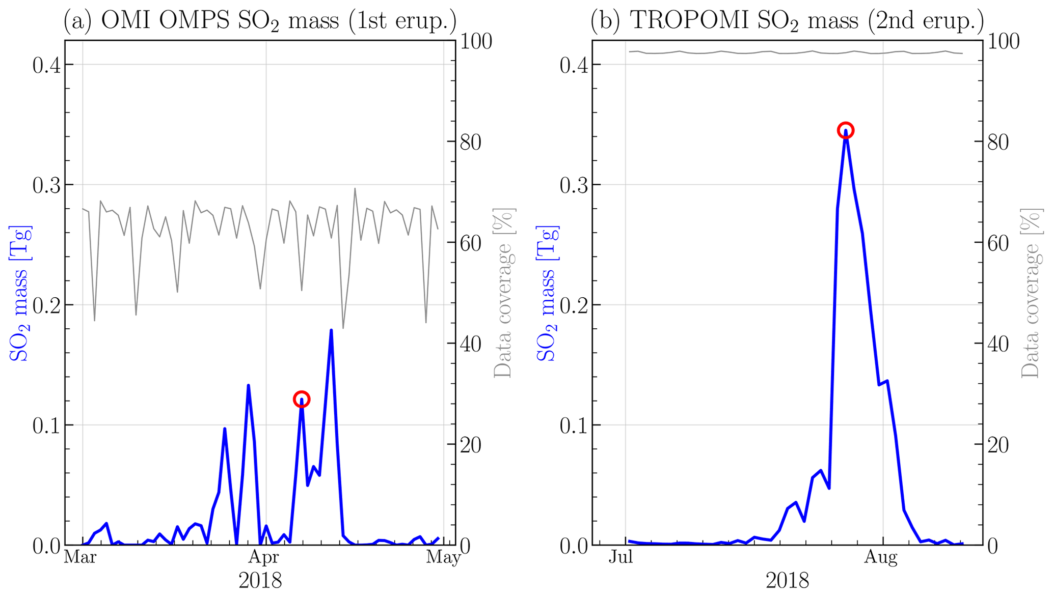
Figure 1The SO2 mass calculated for a threshold of 0.05 g m−2 from the combined OMI and OMPS-NM for the first Ambae eruption in April (a) and from TROPOMI data for the July eruption (b).
The daily OMI and OMPS data were projected on a self-defined grid with a resolution of 0.5∘ and averaged for each segment. The grid dimensions were chosen from 150∘ E to 140∘ W and 10∘ N to 45∘ S for the April eruption. The data were summed up over the entire grid to determine the total SO2 mass for each day in this area. The results for the period from the beginning of March until the end of April 2018 are presented in Fig. 1a with the blue line. The estimate for the day when SO2 reached the stratosphere is marked with a red circle. The daily data coverage in percent, or the percentage of the self-defined grid that contains data that could be used for the analysis, is depicted on the same panel with the gray line. Due to the large data gaps, this SO2 mass is a minimum estimate for the SO2 injected during the eruption.
The largest source of error for estimating the SO2 emission is probably the choice of the assumed SO2 profile because the vertical distribution of the SO2 affects the air mass factor used for the retrieval of the vertical column densities.
3.1.2 TROPOMI data set
The SO2 mass emitted during the eruption of Ambae in late July 2018 was estimated by analyzing SO2 total vertical columns from the TROPOMI instrument (see Sect. 2.6). A grid with a resolution of 0.1∘ in both longitude and latitude was defined from 10∘ N to 35∘ S and 150∘ E to 140∘ W. We utilized sulfur dioxide total vertical columns, assuming an SO2 profile represented by a 1 km thick box filled with SO2 and centered at 15 km altitude, in order to model conditions in an explosive eruption (Theys et al., 2017). Only vertical column densities with values less than 1000 mol m−2 were considered for the analysis. The data above this threshold were excluded because they were considered unrealistic and erroneous. Furthermore, a solar zenith angle less than 70∘ (for the SO2 products that use an SO2 box profile) or a quality value greater than 0.5 (for the SO2 product that uses TM5 model profile), respectively, was required (Theys et al., 2020). The TM5 model is a global chemical transport model that provides a daily forecast of SO2 profiles (Theys et al., 2017). The total vertical column was multiplied by the SO2 molar mass to obtain the SO2 mass loading in the units of g m−2. Afterwards, similarly to Sect. 3.1.1, a threshold of 0.05 g m−2 was applied, and the SO2 mass in units of grams for every grid segment was calculated. Since some orbits overlap, 14 consecutive orbits covering a time span of approximately 24 h were bundled to a data set batch and averaged for each grid segment. Finally, the SO2 masses in all grid segments in the batch are summed up to obtain the total SO2 burden.
The SO2 masses calculated for every batch and for the thresholds of 0.05 g m−2 during the Ambae eruption are presented in Fig. 1b. The date represents the date of the first orbit in each batch that intersects with the area of interest. With the red circle, the day SO2 reached the stratosphere, according to MLS data, is marked, while the data cover is depicted with a gray line. The SO2 mass increased to a maximum of 0.35 Tg on 27 July and declined, by 5 August, to magnitudes of gigagram (hereafter Gg). The SO2 mass for a threshold of 0 g m−2 (not shown) exhibits a high SO2 background of 0.1–0.15 Tg that quickly increases to a maximum of 0.51 Tg on 27 July and decreases to 0.1 Tg on 5 August. The application of a threshold of 0 g m−2 seems to suggest an SO2 background of approximately 0.1–0.15 Tg that is not apparent in Fig. 1 when using a more restrictive threshold. Focusing only on the additional SO2 entry, i.e., the difference between the maximum SO2 and the background emission of 0.1–0.15 Tg, a total burden of approximately 0.35–0.4 Tg SO2 was emitted, applying a threshold of 0 g m−2. This result is comparable to the maximal SO2 burden in Fig. 1.
Furthermore, the calculated maximum of emitted SO2 mass strongly depends on the SO2 data product used. As mentioned in Sect. 3.1.1, the vertical SO2 distribution affects the air mass factor that is used to retrieve the vertical column densities. Assuming a threshold of 0.05 g m−2 and an SO2 profile with the SO2 existing in a 1 km thick box at an altitude of 15 km, as discussed above, results in the maximal SO2 mass of 0.35 Tg. This value increases, respectively, to 0.5 Tg and even to approximately 1.3 Tg by assuming, respectively, a 1 km thick box at an altitude of 7 km and a profile from the TM5 model. These results emphasize the importance of an accurate assumption for the vertical SO2 distribution (see Appendix B).
3.2 OMPS-LP Ext retrieval algorithm
As can be inferred from its name, initially OMPS was designed to obtain ozone products, and in the instrument design, the UV-Vis parts of the spectrum were prioritized. As the prism dispersion is nonlinear, the spectral resolution of the measurements at the wavelength longer than 500 nm degrades exponentially, reaching about 30 nm at 1000 nm. This results in the situation that the usual stratospheric aerosol extinction wavelength 750 nm, used by, for example, SCIAMACHY and OSIRIS (Rieger et al., 2018), is not suitable for use as OMPS-LP measurements around this wavelength are affected by the O2-A absorption band. Thus, for the stratospheric aerosol extinction retrieval, instead of 750 nm, we used the measurements at 869 nm (with a spectral resolution of 22 nm) because the spectral interval from 830 to 900 nm is absorption free.
Even though some aspects of our algorithm have been briefly described in Arosio et al. (2018) and Malinina (2019), here we provide a consolidated summary. The OMPS V1.0.9 aerosol extinction coefficient at 869 nm (Ext869) retrieval algorithm was adapted from the SCIAMACHY V1.4 algorithm (Rieger et al., 2018) and uses the same regularized iterative approach. However, here we used the first-order Tikhonov regularization with the parameter value of 50 to smooth spurious oscillations in the level 1 V2.5 data. Using the information provided by NASA, the signal-to-noise ratio (SNR) is set to 500 for all tangent altitudes.
In V1.0.9, Ext869 is retrieved on a regular 1 km grid from 10.5 to 33.5 km, with the measurement at 34.5 km being used as the reference. Additionally, the effective Lambertian albedo is simultaneously retrieved using the Sun-normalized spectrum at 34.5 km. The retrieval is done under the assumption of stratospheric aerosols being spherical sulfate droplets (75 % H2SO4 and 25 % H2O) with 0 % relative humidity and unimodal lognormal particle size distribution (PSD). In this distribution the median radius (rmed) is equal to 0.08 µm and σ = 1.6; the particle number density a priori profile was chosen in accordance with the Extinction Coefficient for STRatospheric Aerosol (ECSTRA) background climatology (Fussen and Bingen, 1999). We used the refractive indices from the OPAC (Optical Properties of Aerosols and Clouds) database (Hess et al., 1998); for the selected wavelength, the refractive index equals 1.425–1.38597 × 10⁻⁷i. The stratospheric aerosol profile is defined from 10 to 46 km; below and above, the number density profile is set to 0. After the retrieval, the Ext869 values higher than 0.1 km−1 are considered to be cloud contaminated and, thus, are filtered.
The threshold to reject clouds is selected empirically to keep as much as possible of an event associated with increased Ext and reject as many clouds as possible. However, the trade-off between these two factors is determined by the potential application of the data set. For instance, for applications where it is more important to remove as many clouds as possible and single high aerosol peaks are not of a great value, a rather conservative value of 0.002 km−1 is recommended. This value is based on the results from Bourassa et al. (2010), where the Ext750 after the Kasatochi eruption did not exceed 0.001 km−1. This threshold was used in, e.g., Malinina (2019). However, it was noticed that, by implementing the 0.002 km−1 threshold, some profiles with increased aerosol loading were incorrectly filtered for some case studies. Thus, for an investigation of an isolated volcanic eruption, a higher threshold is necessary to preserve all increased Ext values. The 0.1 km−1 value used in this study is based on the experience with the 2019 Raikoke eruption (Muser et al., 2020). For the user's convenience, the products with both cloud filters (0.002 and 0.1 km−1) are provided.
3.3 Comparison of OMPS-LP and SAGE III/ISS
The OMPS-LP Ext869 was originally retrieved to improve the ozone product (Arosio et al., 2018); however, it can also be used to evaluate the changes in stratospheric aerosol loading after volcanic eruptions and biomass burning events (Malinina, 2019). Here, it should be noted that there are three other OMPS aerosol extinction products; two of them are the official NASA Ext675 products, i.e., V1.0 (Loughman et al., 2018) and V1.5 (Chen et al., 2018). Moreover, at the University of Saskatchewan, as a part of the ozone retrieval, a tomographic Ext750 product was obtained (Bourassa et al., 2019). All four Ext products were retrieved at different wavelengths and using different approaches. Thus, their comparison will be not trivial and will contain uncertainties, e.g., associated with Ångström exponent calculations.
In order to evaluate the quality of our Ext869, it was compared with the SAGE III/ISS solar occultation product. There are several advantages to this comparison. First, SAGE III is an independent data set; thus, possible OMPS instrumental issues (e.g., scattering angle dependency) will be revealed by the comparison, which would not be the case when using other OMPS products. Second, SAGE III is an occultation instrument, which means that its Ext profiles are rather precise and independent of the aerosol PSD assumption, in contrast to, for example, OSIRIS. The solar occultation measurements are self-calibrating, and unlike limb instruments, for the Ext retrieval, no assumptions on the aerosol particle size distribution are needed, thus making occultation measurements rather precise.
Another advantage of the comparison with SAGE III is the same measurement wavelength. Both OMPS-LP and SAGE III provide measurements at 869 nm, so no conversion of the aerosol extinction to any other wavelength needs to be done. Even though the spectral resolution of the instruments at this wavelength is different (1.5 nm in SAGE III versus 30 nm in OMPS-LP), it does not influence the aerosol extinction coefficient strongly because the wavelength interval from 830 to 900 nm is absorption free.
For the comparison, individual profiles from 7 June 2017 until 31 August 2019 were used. The profiles were collocated using the following criteria: the difference between the profile's coordinates should be less than 2.5∘ in latitude, 10∘ in longitude, and 24 h in time. The minimal time difference between profiles was 01:47:37 h, while the maximum difference is 22:07:38 h. Overall, there are 19 264 collocated measurements used for this comparison. For SAGE III data, similarly to OMPS, the aerosol extinction values higher than 0.1 km−1 were filtered out. Additionally, the SAGE III Ext869 values were excluded if the uncertainty provided by NASA is higher than 50 %. We did not filter negative Ext869 because this would bias the comparison (see Damadeo et al. (2013) for details).
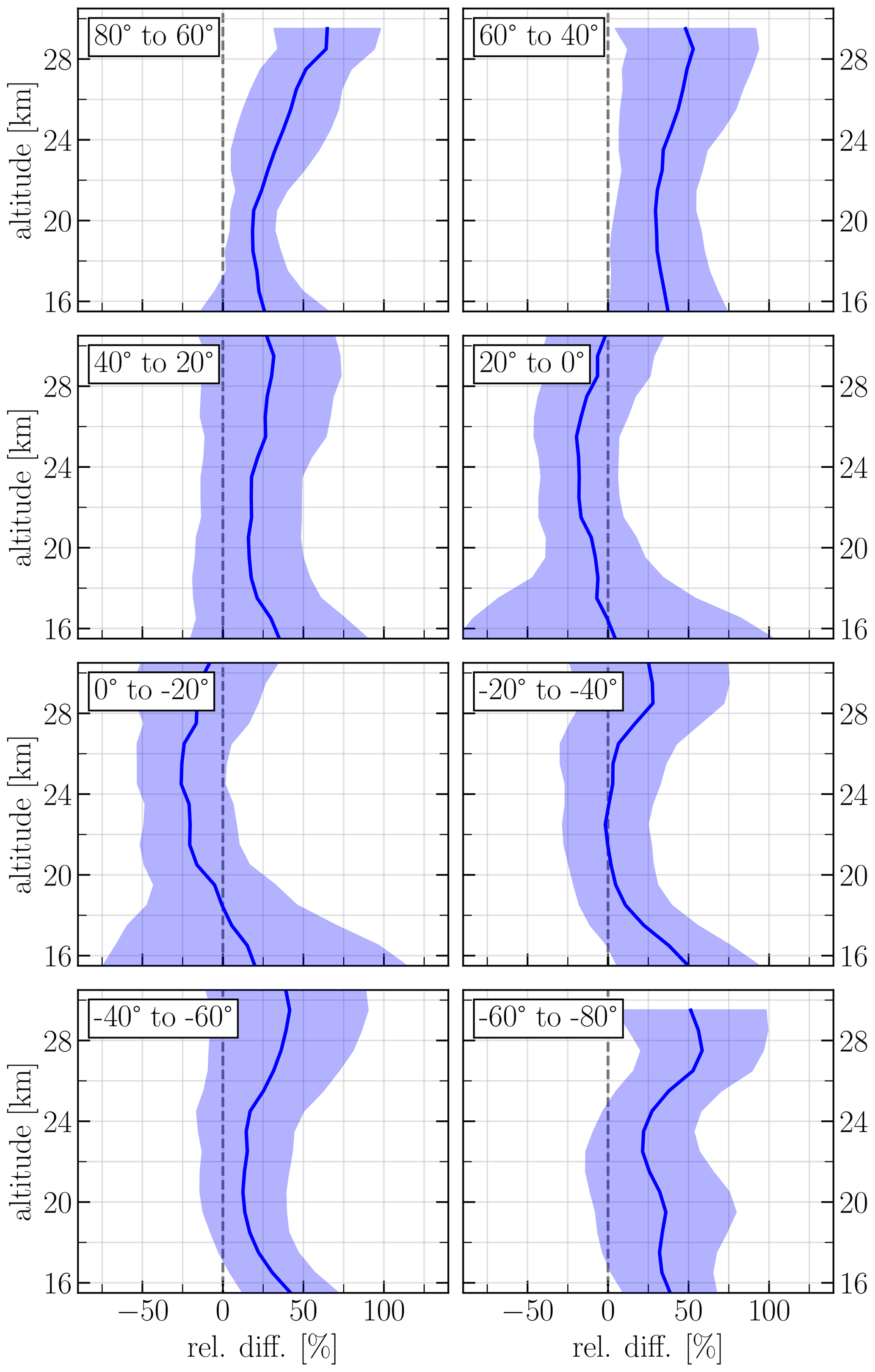
Figure 2Mean relative difference in Ext869 between OMPS-LP and SAGE III/ISS calculated as 200 × (OMPS-SAGE)/(OMPS+SAGE). The shaded areas show ± 1 standard deviation.
The mean relative differences between OMPS and SAGE III Ext869 are presented in Fig. 2 in 20∘ latitude bins. For most of the altitudes in all latitude bins, the relative difference is within 25 %. In the tropical and midlatitudes, the only exceptions are the altitudes below 18 km, where, despite filtering, the influence of clouds is still present. The largest differences are observed in high latitudes (40∘ to 80∘ in both hemispheres), in particular at the altitudes above 24 km. For example, at about 28 km altitude, the differences reach up to 60 % in these latitude bins.
Generally, the above-described differences are similar to the relative differences between SCIAMACHY V1.4, OSIRIS v5.07, and SAGE II v7 (Rieger et al., 2018; Malinina, 2019). Additionally, Chen et al. (2020) showed that the differences seen between the OMPS Ext675 V1.5 and SAGE III product have the same shape and order of magnitude. Rieger et al. (2018) studied precisely the reasons for the observed differences. Since the OMPS V1.0.9 algorithm is very similar to the SCIAMACHY V1.4 algorithm used in that study, and since the OMPS and SCIAMACHY have very similar geometries, the same explanations, as given by Rieger et al. (2018), are appropriate. According to this study, the most important sources of errors in limb retrievals arise from the uncertainly assumed aerosol loading at the reference tangent altitude and the unknown aerosol particle size distribution parameters. The latter factor mostly affects the high latitudes where the viewing geometries are close to forward and backward scattering.
Based on our comparison and the results from the other limb-occultation instrument studies, it can be concluded that our OMPS V1.0.9 Ext869 is of sufficient quality to be used for scientific purposes.
3.4 OMPS-LP aerosol extinction climatology
In order to study the aerosol extinction coefficient evolution after a volcanic eruption, the OMPS V1.0.9 product has to be averaged in some fashion. We have created two level 3 products, which are monthly and 10 d averaged Ext869. Both products were binned onto a regular geographical grid with 2.5∘ latitude and 5∘ longitude steps. Since the retrieved product is provided on the regular 1 km grid, no vertical averaging is needed.
Table 1Volcanic eruptions and biomass burning events shown in Fig. 3.
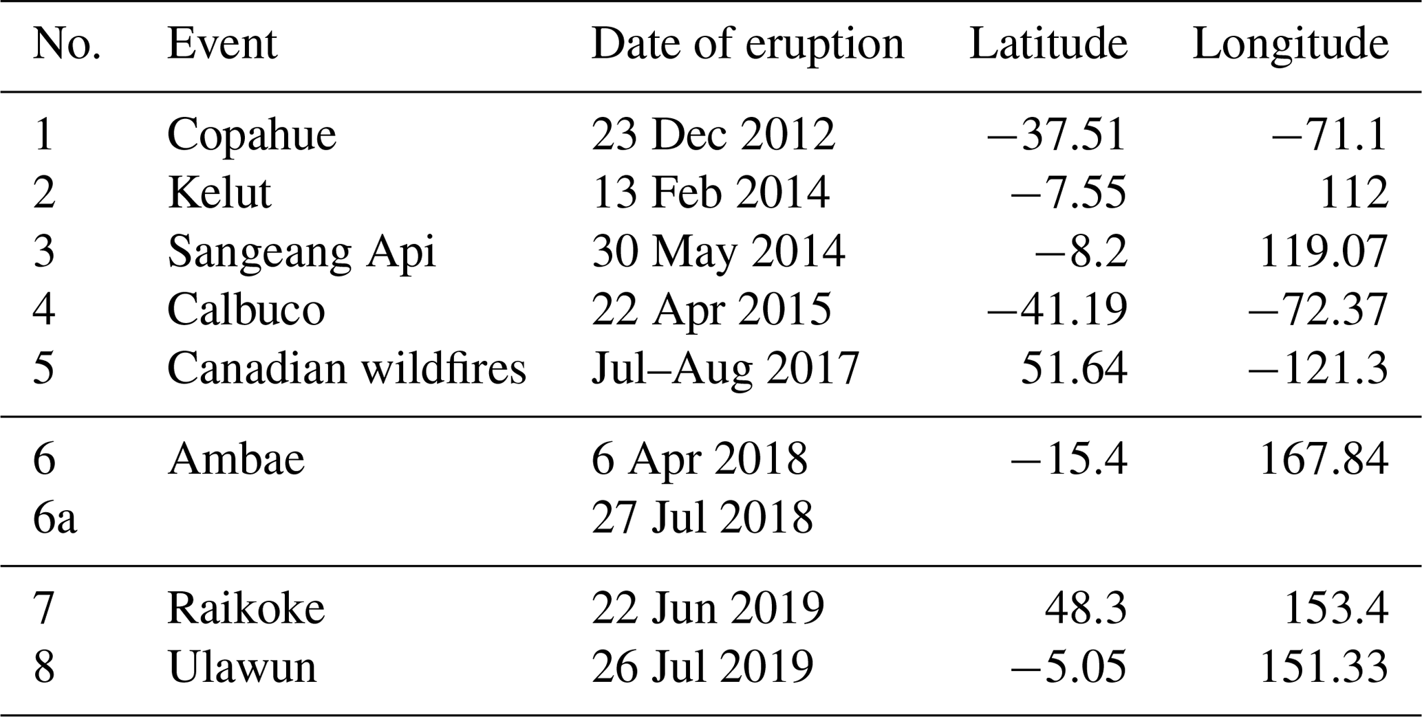
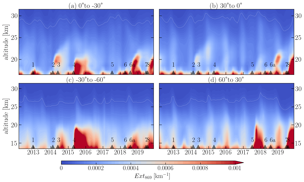
Figure 3Monthly mean aerosol extinction coefficient (Ext869) distribution as a function of time and altitude. The values were obtained by binning and zonally averaging OMPS-LP monthly level 3 Ext869. The white lines show 0.00005 km−1 Ext869 level. The triangles with numbers represent volcanic eruptions and biomass burning events (see Table 1).
An example of zonal monthly mean Ext869 averaged in 30∘ latitude bins for the whole OMPS operation period is presented in Fig. 3. In this figure, the volcanic eruptions and a relevant biomass burning event are shown with gray triangles with numbers. The information on the volcanic eruptions is presented in Table 1. We show only Ext869 within 60∘ in both hemispheres because, as it was pointed out in Sect. 3.3, the aerosol extinctions above these latitudes are associated with larger uncertainties. Furthermore, the main scope of this paper is to study the tropical Ambae eruptions; thus, we do not focus our attention on aerosol loading in the high latitudes.
Analysis of Fig. 3 shows that there is a certain increase in Ext869 at the very beginning of OMPS operation in the Northern Hemisphere in the bin between 60∘ and 30∘. This is associated with the eruption of Nabro (13∘ N) in the middle of 2011. Additionally, one can see an increase in Ext869 some time after the eruptions in Table 1 and from the Canadian wildfires of 2017 (number 5 in Fig. 3 and Table 1). The degree of the enhancement, and the time lag between the eruptions seen in the latitude bands, are dependent on the volcano's location and the eruption strength. Usually, for the tropical eruptions, an increase in stratospheric aerosol loading is seen globally because the aerosols and precursors are transported with the Brewer–Dobson circulation (BDC) to both hemispheres. Also, in the Tropics, the BDC is responsible for the tape recorder effect or the delayed increase in Ext869 with height (Vernier et al., 2011). For example, in Fig. 3a and b, the tape recorder effect is seen for the Kelut, Sangeang Api, Calbuco, and Ambae eruptions, as well as for the Canadian wildfires. For the eruptions in the midlatitudes, the increase usually stays in the hemisphere where it occurred (e.g., Oman et al., 2006; von Savigny et al., 2015; Toohey et al., 2019; Malinina, 2019).
Another readily identifiable feature in Fig. 3 is the periodical increase in Ext in all latitude bins. There are several drivers causing this pattern. The annual seasonality, which is seen as yearly reoccurring lighter colored stripes, in both Tropics and midlatitudes is related to two factors. First, there are some yearly changes in stratospheric aerosol loading (Hitchman et al., 1994; Bingen et al., 2004). Second, for the limb-viewing instruments, an important factor is the seasonality in solar scattering angle, which leads to artifacts of the retrieval predominately in the extratropical regions (see, e.g., Rieger et al., 2018). Additionally, for the tropical region, there is a periodic signal above 25 km altitude associated with the quasi-biennial oscillation (QBO). It can be seen in the thin white line, which represents the 0.00005 km−1 Ext869 level. However, as with the other altitudes, this Ext869 level is somewhat affected by the annual variation in addition to the QBO. Here, it is important to mention that, during the OMPS operation period, two QBO disruptions were reported, namely in 2015–2016 (Newman et al., 2016) and 2019–2020 (Kang and Chun, 2021). These disruptions might also mask the changes in the high-altitude extinctions. Generally, the influence of the QBO on stratospheric aerosols is well known and was previously reported by, e.g., Vernier et al. (2011); Hommel et al. (2015); Brinkhoff et al. (2015); von Savigny et al. (2015); Malinina et al. (2018).
One should also mention the increase in the extinction at approximately 16.5–17 km in Fig. 3a and b and at around 13.5–15 km in Fig. 3c and d. These are the residual clouds which were not filtered by our threshold. Though we show the data in Fig. 3 above the average tropopause height for the bin, some overshooting convective clouds still could be present and influence an average Ext. Here we want to highlight that we are aware of disadvantages of our fixed cloud filtering threshold, which can also be considered quite high. As we state above in Sect. 3.2, our previous threshold was too low and was filtering out parts of volcanic and forest fires plumes. Furthermore, any fixed threshold would either filter out some high-extinction events or leave some fractions of cloud in. However, the other commonly used cloud filtering approach exploiting altitude derivative of spectral ratio also suffers from poor discrimination under certain conditions (Chen et al., 2016; Rieger et al., 2019).
4.1 Aerosol extinction coefficient evolution
As it was highlighted in the introduction, Ambae was one of the largest eruptions of the last decade but has not been a focus of scientific or public interest. The eruptive period, which lasted over a year, had two explosive phases when SO2 was injected into the stratosphere (the exact information on SO2 mass estimation can be found in Sect. 3.1). The first emission was smaller, and the perturbation in Ext869 did not reach altitudes above 21 km (see Fig. 3a and b). The second emission was considerably larger; it perturbed Ext869 up to 23.5 km in the Tropics and up to 22 km in the extratropical regions. However, to better evaluate the plume evolution, we will further analyze 10 d averaged Ext869.
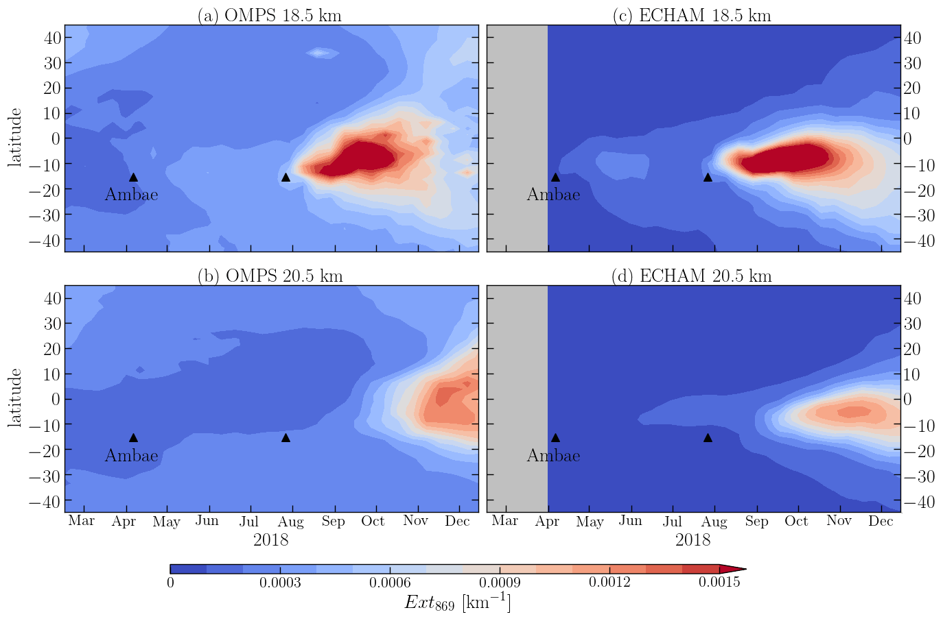
Figure 4The evolution of the aerosol extinction coefficient (Ext869) at 18.5 and 20.5 km altitude after the Ambae eruptions of 2018. In panels (a) and (b), Ext869 was retrieved from OMPS-LP measurements; for panels (c) and (d), Ext869 was modeled by MAECHAM5-HAM. Both data sets were averaged over 10 d periods.
4.1.1 Ambae eruption as seen by OMPS-LP
The evolution with time and altitude of the 10 d averaged zonal mean Ext869 at 18.5 and 20.5 km is presented in Fig. 4a and b. Foremost, it should be noted that the increase in Ext869 in February–May 2018 in the latitudes above 25∘ N at 18.5 km and above 7∘ N at 20.5 km is related to the disappearing plume from the Canadian wildfires of 2017. Already in the first week after the eruption a small increase in Ext869 is seen around the Ambae location; however, this increase cannot be uniquely attributed to the Ambae eruption and can be caused by the transport of the aerosol from preceding events. The more significant increase is observed in early May 2018. At the time, the plume is located around 10–25∘ S and stays there until late June. In June, the increase in Ext869 starts to spread to the south, reaching 35–45∘ S in July 2018. At 20.5 km, the increase after the first SO2 release is rather negligible. Nevertheless, there is still an area with the increased aerosol loading below 20∘ S from the beginning of May.
In late July 2018, during the fourth phase of the eruption, Ambae injected another portion of ash and SO2. Almost at the same time, Ext869 increases at 18.5 km directly at the source. In about 2 weeks, the volcanic plume starts to spread both northward and southward and is located between the Equator and 35∘ S in early September, reaching 45∘ N in November–December 2018. The southern border of the plume at 18 km is harder to identify because it mixes with the aerosol from the previous SO2 release. However, an increased aerosol loading is observed to the south of 35∘ S in September and intensifies further with the time. By mid-October 2018, at 18.5 km, the plume shows a clear reduction around the Equator and continues to weaken with time. At 20.5 km, the plume appears in mid-September 2018 at around 10∘ S and spreads northwards and southwards from that moment on, reaching its maximum in November. It is located in between 30∘ S and 35∘ N in mid-December 2018. Again, at the southern border of the plume, there is an area of increased Ext869, which is related to both eruptions.
4.1.2 Ambae eruption modeled by ECHAM
The Ambae experiment setup used the estimated SO2 emissions from Sect. 3.1 and the injection altitudes from MLS data (see Appendix A). As pointed out, the result of the calculated SO2 mass from OMI/OMPS data for the April eruption provides only a minimum estimate because the analysis suffered from large data gaps. In accordance with Kloss et al. (2020), an SO2 mass of 0.12 Tg was chosen as a realistic assumption for the April eruption in the simulation. Thus, we injected 0.12 Tg SO2 at altitudes of 82 to 102 hPa on the 6 April for 4 h and 0.36 Tg SO2 at altitudes between 74 and 90 hPa on 27 July for 24 h, starting at 18:00 UTC (universal coordinated time). During the review process, the extension of the self-defined grid for the TROPOMI analysis was reduced to exclude SO2 artifacts at the borders, which resulted in a slight decrease in the estimated SO2 mass from 0.36 to 0.35 Tg. The ECHAM simulations were carried out with the former value, but we do not expect a significant impact due to that difference. The long eruption phase was chosen to take the observed series of eruptions into account. To slow down the oxidation of SO2 due to the limited availability of OH in a volcanic cloud (Mills et al., 2017), the concentration of OH was limited in the first days after the eruption, i.e., day 1 to 10 was limited to 40 % and day 10 to 20 to 60 % of the prescribed OH. The sea surface temperature (SST) is set to a climatological value (Hurrell et al., 2008).
In order to be consistent with OMPS-LP measurements, the output of ECHAM was interpolated to the same vertical grid as provided by OMPS-LP. ECHAM provides Ext at 550 and 825 nm; thus, for consistency in the comparison, the simulated Ext was recalculated to 869 nm, and afterwards, the 10 d averages were calculated. The simulated distribution of Ext869 with time and latitude at 18.5 and 20.5 km is presented in Fig. 4c and d. In these panels, it is seen that, at 18.5 km, the aerosol extinction coefficient starts to increase almost right after the first eruption and reaches its peak in May. The majority of the volcanic aerosol stays in the Tropics between 30∘ S and the Equator. A small amount of aerosol is dispersed meridionally right after the eruption. After the second eruption, at the end of July, the first aerosol is formed right after the eruption, with Ext increasing slowly until it reaches the maximum in September. Most aerosols are located to the south of 10∘ N. In the last days of September, the plume is still very well pronounced, and it starts to spread meridionally, mostly southwards. By beginning of October, Ext increases also in the Northern Hemisphere at 20∘ N; this increase spreads with the time to 40∘ in the late December. The plume starts to weaken at the beginning of November.
At 20.5 km, the plume from the first eruption appears in late June. The plume at this altitude is quite weak and does not extend much over the latitudes. Basically, it is a small area in between the Equator and 10∘ S. The increase in Ext associated with the second eruption appears at 20.5 km in very late August; by the middle of September, the plume intensifies and starts to expand meridionally. It reaches its maximum by November, when the increase is seen from 10∘ N to 40∘ S. From that moment, the plume starts to slowly disappear. In late December, the Ext increase is seen from 30∘ N to 45∘ S.
4.1.3 Discussion
In order to evaluate the consistency of the results from OMPS and ECHAM, the panels in Fig. 4 need to be compared. It is obvious that the model and the observations are very close to each other, in particular at 18.5 km. The plume from the first eruption appears and intensifies at the same time at 18.5 km; however, in the model it is weaker, and it reaches 20.5 km about a month later. This is most likely related to the fact that, in the model, neither the anthropogenic nor biomass burning sources are taken into account.
The Ambae plume from the July eruption looks even more similar in the model results and measurements. Not only does the plume appear at the same time, at 18.5 km, and is located at the same latitudes, but also both model and measurements show a wave-shape of the plume. The curvature in both plumes appears in mid-September; however, in the OMPS-LP data, the plume is bending stronger to the north. It should also be noted that the ECHAM simulations show a more intensive and longer living plume at this altitude. Additionally, in the OMPS-LP data, in the second part of October, the aerosols move north- and southward evenly, while in the ECHAM data, the plume is instead transported to the south. In ECHAM data at 20.5 km, the July plume appears about 2–3 weeks earlier than in the OMPS measurements. Though the intensity of the modeled plume at this altitude is slightly weaker, the absolute differences are smaller than at 18.5 km. However, the horizontal distribution of the modeled plume is less consistent with the measurements. While the plume in ECHAM data stays, with the time, in the same latitude band mostly in the Southern Hemisphere, in the OMPS data, it has a C-shape around the Equator.
It should be highlighted that, even though there are some differences between the modeled and measured Ext, the consistency is quite remarkable. There are key main factors which contributed to this particular agreement between OMPS and ECHAM, namely, rather precise SO2 mass and height estimation, as well as nudging of meteorological data. Consequently, it is seen that the second plume, whose emission was estimated from TROPOMI data, was modeled more accurately. At the same time, our internal studies showed that the ECHAM SO2 sensitivity plays a key role in the lifetime and distribution of the plume (see Fig. S1 in the Supplement).
It is a well-known feature of ECHAM that the meridional transport is too strong, causing a relatively short lifetime of sulfate (e.g., Niemeier et al., 2009), especially compared to results of other models (e.g., Marshall et al., 2018). Therefore, the nudging of the meteorological data provided a realistic transport pattern resulting in good agreement with OMPS-LP measurements. However, the nudging database, the ERA5 reanalysis, has not only observational but also a strong model component as well. Thus, small differences with observations are rather possible, especially in the stratosphere. Additionally, the stratospheric aerosol layer is close to the ozone layer at 24 km. ECHAM uses the prescribed ozone and OH values which do not change due to the presence of volcanic aerosol.
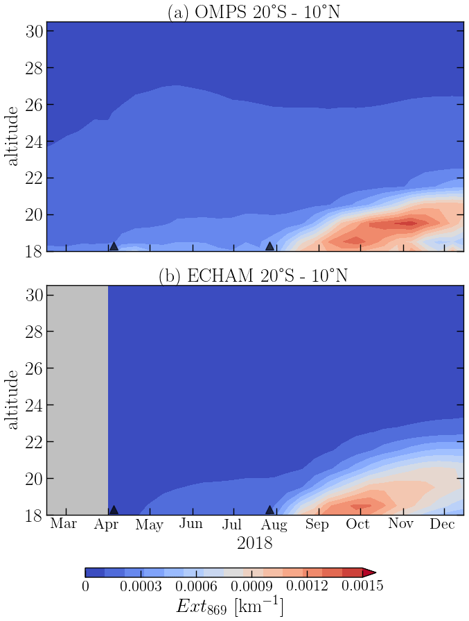
Figure 5Evolution of zonal mean aerosol extinction coefficient (Ext869) in the Tropics (20∘ S–20∘ N), with altitude and time after the Ambae eruptions of 2018. In panel (a), the data from OMPS-LP are presented, and in panel (b) the simulation with MAECHAM5-HAM is plotted. Both data sets were averaged over a 10 d periods.
Another way to assess the degree of consistency between the model and the measurements is to analyze the vertical distribution of Ext with the time (see Fig. 5). Since most of the plume stayed in the tropical region, for Fig. 5, the OMPS (Fig. 5a) and ECHAM (Fig. 5b) Ext were averaged between 20∘ S and 10∘ N. In this figure, it is again obvious that, in the model, the perturbation from the volcano reached the same altitudes. Additionally, it is observed that the plume was weaker for the April eruption. However, consistency for the second eruption is again striking. The plume has the same overall shape and is located at the same time coordinates. A disagreement is seen, however, around the 19.5 km altitude in November, where OMPS-LP data show an increased extinction not present in ECHAM simulations. Also, Kloss et al. (2020) report maximum extinction in the 18–19 km layer in November when analyzing OMPS-LP data. The reasons for the observed disagreements are still under investigation.
4.2 Radiative forcing
In order to assess the RF from the Ambae eruption, we analyzed the top-of-the-atmosphere ECHAM RF output and the top-of-the-atmosphere RF calculated from OMPS-LP measurements. For the latter, we use the empirical approximation given by Eq. (1), as suggested by Hansen et al. (2005) the following:
where τ550 is the stratospheric aerosol optical depth at 550 nm. Although originally proposed for the globally averaged model data, Eq. (1) was successfully used for the RF assessment from the measurement results (see, e.g., Solomon et al., 2011; von Savigny et al., 2015). As the focus of our study is on the additional RF after the tropical Ambae eruptions, we do not consider global averages but limit the comparison to 20∘ S–20∘ N region.
To apply Eq. (1) to the OMPS-LP data, we determined τ550(869) by integrating the Ext869 from instantaneous tropopause height to 33.5 km and then converting the result to 550 nm wavelength by using an Ångström exponent of 2.47, which is appropriate for the particle size distribution used in the Ext869 retrieval (see Sect. 3.2). The tropopause height values were obtained for each single OMPS-LP measurement by using corresponding ECMWF-ERA5 temperature profiles. The World Meteorological Organization (WMO) definition of the tropopause, based on the temperature lapse rate, was implemented (WMO, 1957), and the tropopause height calculation algorithm follows the one from Appendix A (1) of Maddox and Mullendore (2018). Afterwards, the τ550(869) values were averaged over 10 d period. For consistency, we also applied Eq. (1) to the ECHAM τ. Additionally, from all data sets, mean tropical τ in the period from 1 April to 19 July 2018 was subtracted to remove the effects of background aerosol. Even though the chosen period contains the effects of the first weaker Ambae eruption, it is a common cleaner period available for all data sets and, thus, is considered to be optimal for the study.
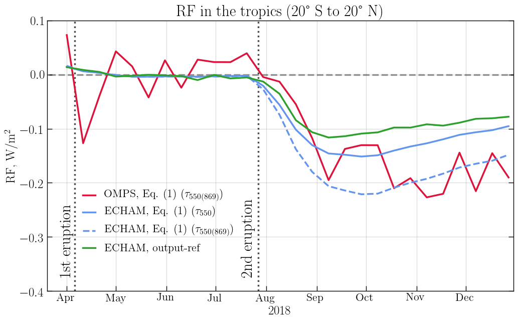
Figure 6The radiative forcing (RF) from ECHAM and OMPS-LP averaged over the Tropics (20∘ S–20∘ N). The green line shows the difference between ECHAM instantaneous RF calculated accounting for and neglecting the Ambae eruptions. Red and blue lines show, respectively, the RF calculated with Eq. (1) from OMPS-LP τ869 converted to τ550(869), and ECHAM τ550 (blue solid) and ECHAM τ869 converted to τ550(869) (blue dashed). From all data sets, the respective mean RF in the period from the 1 April to the 19 July 2018 was subtracted.
The normalized RFs are presented in Fig. 6. Here, the tropical instantaneous top-of-the-atmosphere all-sky RF, calculated as an anomaly to a control simulation without the Ambae eruption, is presented with a green line as a function of time. The OMPS-LP RF, calculated employing Eq. (1), is shown with a red line. To illustrate the validity of Hansen's formula to a non-global data set, it was also applied to the τ550 obtained directly from the ECHAM model. The result is shown with the solid blue line in the figure. The influence of the assumed particle size distribution on the Ext and/or τ conversion to a different wavelength is illustrated by the recalculation of ECHAM τ869 to τ550(869), using the fixed Ångström exponent as it was done for OMPS-LP. The instantaneous RF resulting from Eq. (1) applied to ECHAM τ869 converted to τ550(869) is presented with a dashed blue line in Fig. 6. Both dates of Ambae eruptions are marked with vertical dotted gray lines.
Analyzing Fig. 6, it becomes obvious that the effect of the first smaller Ambae eruption is negligible for the RF. All four lines show almost no temporal change between the eruptions (1 April to 27 July 2018) and are located around 0 W m−2. Even though the RF for the period was subtracted from all data sets, it was a mean value, resulting in temporal behavior being unaffected by this normalization. After the second eruption, all four lines drop significantly. The ECHAM instantaneous RF (green line) reaches its maximum of −0.11 W m−2 in the first week of September, and afterwards the RF declines slowly up to −0.08 W m−2 by late December 2018. The solid blue line, or the RF calculated with Eq. (1) from ECHAM τ550, has very similar behavior with the green line; however, it reaches its maximum (−0.13 W m−2) in late September and keeps the offset from the green line by ≈ 0.02 W m−2 until the end of 2018. The calculated RF from ECHAM τ550(869) reaches its maximum at the same time as the solid blue line, but its absolute value is significantly larger (−0.22 W m−2). Further with time, the offset between the dashed and solid blue lines becomes somewhat smaller, reaching a value of 0.05 W m−2 in December. At the same time, the red line showing the RF calculated with Eq. 1 from OMPS-LP drops heavily after the second eruption but becomes noisier from September on. The maximum in RF (−0.22 W m−2) is observed in November 2018, which is in agreement with the maximum of the extinction coefficient seen in Fig. 5a. The OMPS-LP RF decreases afterwards to about −0.19 W m−2 by the end of the year.
In the discussion of Fig. 6, it is important to draw the reader's attention to the offset between the ECHAM RFs calculated with Eq. (1) from τ550 and τ550(869). After the second eruption, the difference reaches up to 70 %. This difference is a prime example of the influence of assumed particle size distribution parameters on the RF calculations. For example, at the plume maximum, the difference is almost as large as the forcing, but it decreases while the stratosphere relaxes. In spite of these discrepancies, the respective similarities of the ECHAM τ550(869) and OMPS-LP RFs (dashed blue and red lines), as well as ECHAM τ550 and ECHAM output (solid blue and green lines), are remarkable. Here it should be noted that, although there are obvious differences between the curves, they generally have quite good temporal correlation and capture the second eruption very well.
Combining the abovementioned facts, the following conclusions can be drawn. Even when applied to the tropical region rather than globally, Hansen's formula given by Eq. (1) provides a reliable approximation of RF with about 20 % accuracy. In turn, the τ conversion to a different wavelength is a more significant source of uncertainty with a potential to increase the estimated RF by up to 70 %. After accounting for those uncertainties, a very good agreement between the RF values from ECHAM and those from OMPS-LP is observed. For the particular Ambae eruption studied in this paper, using Hansen's formula, we estimate the tropical RF caused by an increase in stratospheric aerosols to be about −0.13 W m−2.
The value obtained for the Ambae RF in this study is significantly lower than that reported by Kloss et al. (2020). In our opinion, the main reason for the disagreement is how the non-Ambae signal is subtracted. By subtracting the radiative forcing just before the second eruption, we ensure that only the Ambae contribution is accounted for. On the contrary, Kloss et al. (2020) use some background aerosol scenario, which is not clearly described in their paper, to remove other contributions than that of Ambae. Another issue can be related to the definition of the tropopause. Although it is not stated clearly, from the remark “(full profiles, for the whole stratosphere)” in Kloss et al. (2020), we guess that only the stratospheric part of the aerosol profile is used to calculate the radiative forcing, i.e., the same approach as that used in our study. If our guess is wrong and Kloss et al. (2020) use the tropospheric part of the profiles as well, then this might be a reason for the observed disagreement. Otherwise, there might still be a difference in the definition of the tropopause and thus in the calculation of the lowermost altitude in the stratosphere. Kloss et al. (2020) do not provide the definition of the tropopause they use, which complicates a direct comparison. There are also some general issues associated with the calculation of small differences of two large values (i.e., radiative forcing from the fluxes) when using a radiative transfer model. These are related to adequate gridding (altitude, streams, Fourier terms, and solar zenith angles), the possible need to account for the atmospheric sphericity for the scattered light (i.e., going beyond the pseudo-spherical solution), and the possible implications of using a simple parametrization of the aerosol scattering with an asymmetry parameter.
The distribution of aerosol extinction coefficients at 869 nm in the stratosphere after the 2018 Ambae eruption was compared using the data retrieved from the OMPS-LP observations and that modeled by ECHAM.
We present here the retrieval algorithm (V1.0.9) of stratospheric aerosol extinction coefficient profiles at 869 nm from the OMPS-LP instrument. The retrieval algorithm was adopted from SCIAMACHY V1.4 and shows similar results in comparison with solar occultation instruments. The comparison of the OMPS V1.0.9 product with the aerosol extinction coefficient observations from SAGE III/ISS showed that the mean relative difference is less than 25 % for the profiles between 40∘ S and 40∘ N. In the higher latitudes, the difference is somewhat larger; it is less than 35 % below 25 km but can reach about 60 % at 28 km.
We also show the changes in the aerosol extinction coefficient after the 2018 Ambae eruption using monthly mean and 10 d average data. Ambae caused one of the largest perturbations in the aerosol layer for the OMPS operating period. Volcanic aerosols rise over time to about 21 km in the Tropics within the tropical pipe of BDC (the tape recorder effect). Analyzing the 10 d average data, it has been observed that the plume from the first phase of the eruption was relatively weak and did not spread outside the Tropics. The second eruption in July was much larger, and the aerosols also spread to the midlatitudes of both hemispheres.
The measurement data were compared with the model output from a GCM with coupled aerosol microphysics (ECHAM). In order to simulate the Ambae eruption accurately, the injected SO2 emission was estimated using combined OMPS and OMI data for the April eruption (0.12 Tg) and TROPOMI data for the July eruption (≈ 0.36 Tg). The altitudinal distribution of the SO2 was assessed using MLS profiles. Thus, the resulting simulation showed that the model and measurements agree well with each other. The main differences concern the intensity and the lifetime of the volcanic perturbation. For the first eruption, ECHAM underestimated the strength of the plume as well as the time by which it reaches 20.5 km of altitude, whereas for the second eruption the modeled plume reached higher altitudes about 2–3 weeks earlier, and the plume lived longer while being slightly weaker overall at those altitudes. Although the differences between the measured and modeled plumes exist, they are rather minor, and the consistency is remarkable. The good agreement is explained by the rather precise SO2 injection mass and height assessment, as well as by the nudging of meteorological data.
We also compare the top-of-the-atmosphere radiative forcing (RF) in the Tropics caused by the increase in stratospheric aerosol loading from the second Ambae eruption. While the time evolution of RF from the ECHAM output and ECHAM and OMPS-LP stratospheric aerosol optical depths generally agree quite well, the absolute values vary significantly. The empirical formula used in our assessment works well not only for the globally averaged aerosol optical depths but also for the tropical region. However, this approach suffers from the errors associated with the assumed particle size distribution for the data sets where the Ångström exponent has to be used to convert stratospheric optical depth to another wavelength. We estimate the RF in the Tropics after the second 2018 Ambae eruption to be about −0.13 W m−2.
In general, if the initial data (SO2 mass, day, and height of injection, as well as meteorological data) are quite precise, the model gives a very good estimate of the plume distribution, and the calculation of the radiative forcing can be made for an isolated plume without additional assumptions. Overall, the best results can be achieved only by combining observational data and modeling capabilities. Thus, it is very important to unite the measurement and model community together, for example, as the research unit VolImpact does (von Savigny et al., 2020).
As it was pointed out in Sect. 3.1, in order to find out SO2 injection heights, we used MLS (Sect. 2.4) SO2 number density profiles. Using the plume locations from the nadir instruments, OMI/OMPS-NM for the April eruption, and TROPOMI for the July eruption, we determined the days on which the SO2 reached UTLS. We show these profiles in Fig. A1. For the first eruption, which happened on 6 April 2018, the profiles are depicted in blue, while the profiles for the second eruption on 27 July 2018 are red. The individual profiles in the plume are plotted with thin lines, while the average profile for the area are shown by the thicker line. On 6 April, the SO2 cloud was located between 15 and 17 km. The tropopause height, according to the MLS data, was between 16.7 and 17.5 km for the Ambae plume location. For 27 July, the SO2 cloud was detected in between 15 and about 18 km, while the tropopause height was located between 15.9 and 16.5 km. We used this information to simulate the Ambae eruption with ECHAM, and the results were presented in Sect. 4.1.2.
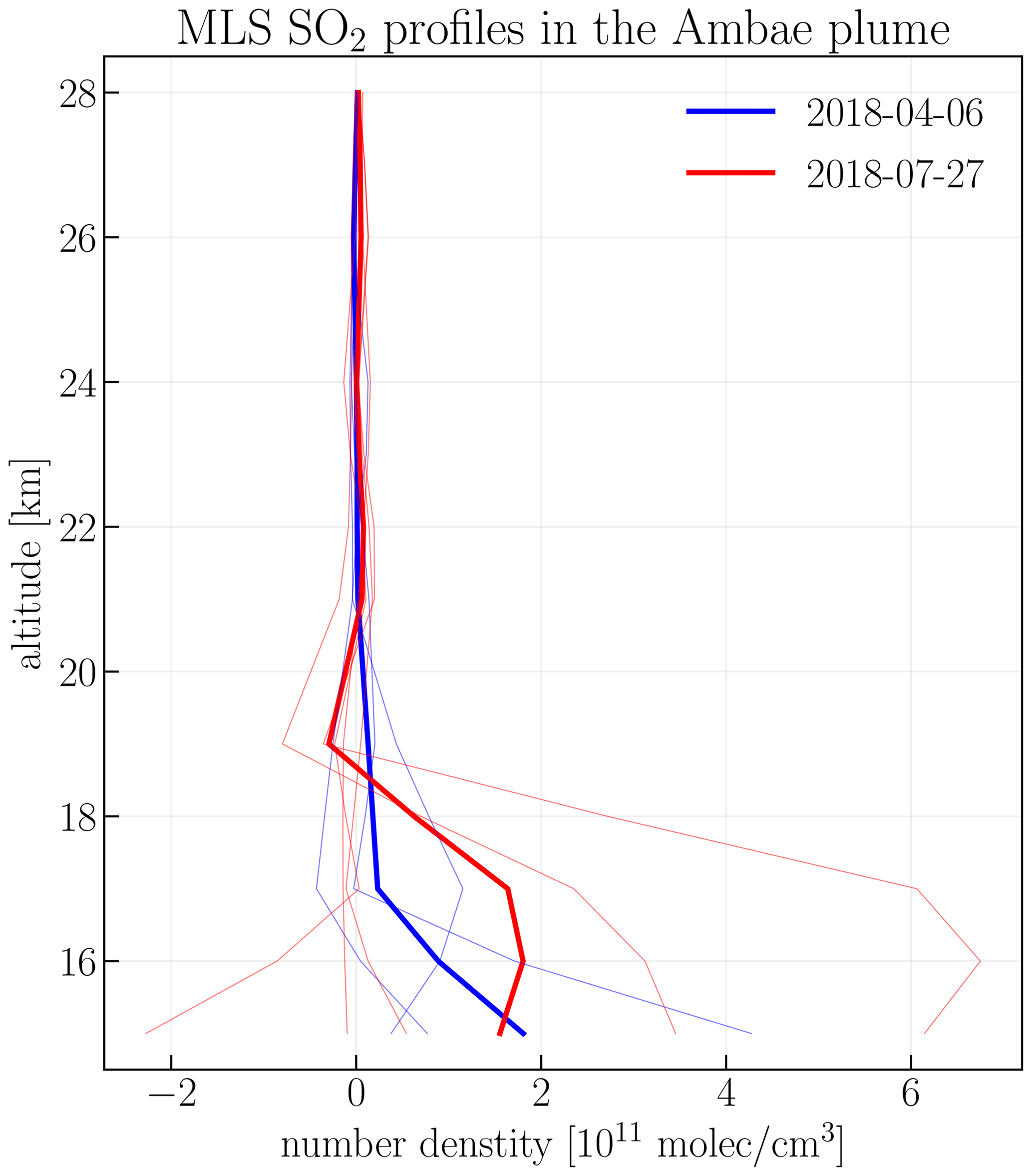
Figure A1MLS SO2 number density profiles in the Ambae plume on 6 April (blue lines) and on 27 July (red lines) 2018. The thick lines show mean profile, while thin lines depict individual measurements within the plume.
The estimate of the ejected SO2 mass during the Ambae eruption depends strongly on the assumed SO2 profile. TROPOMI satellite data provide the total SO2 vertical column densities for three different box profiles that assume an SO2-filled 1 km thick box centered on ground level at 7 km and in 15 km altitude above sea level, respectively. To illustrate the importance of the profile choice, the SO2 mass for the 2018 July Ambae eruption was calculated using TROPOMI data that either assume an SO2 box profile at 7 or 15 km altitude above sea level A threshold of 0.05 g m−2 was applied, and the results were presented in Fig. B1, where the blue line shows the estimates for 15 km profile, and the green line depicts the estimates for 7 km profile. The calculated SO2 mass clearly differs, with the maximum value of 0.35 Tg for the 15 km box profile being smaller than the estimate of 0.5 Tg for the 7 km box profile.
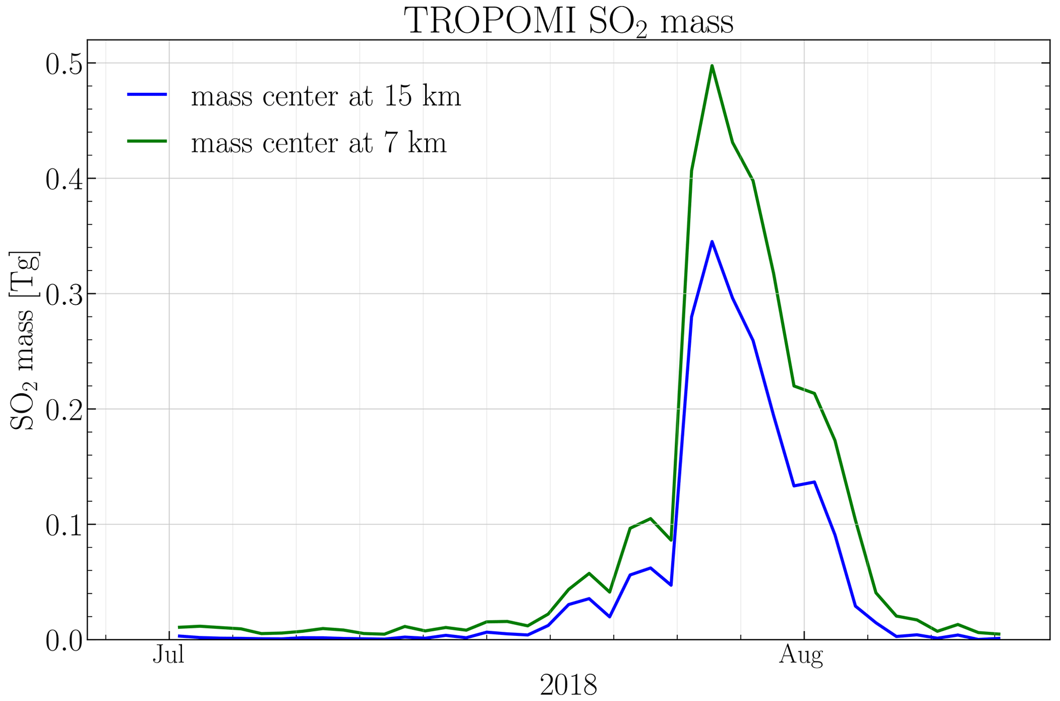
Figure B1SO2 mass from TROPOMI for the 7 km (green line) and the 15 km (blue line) SO2 profile.
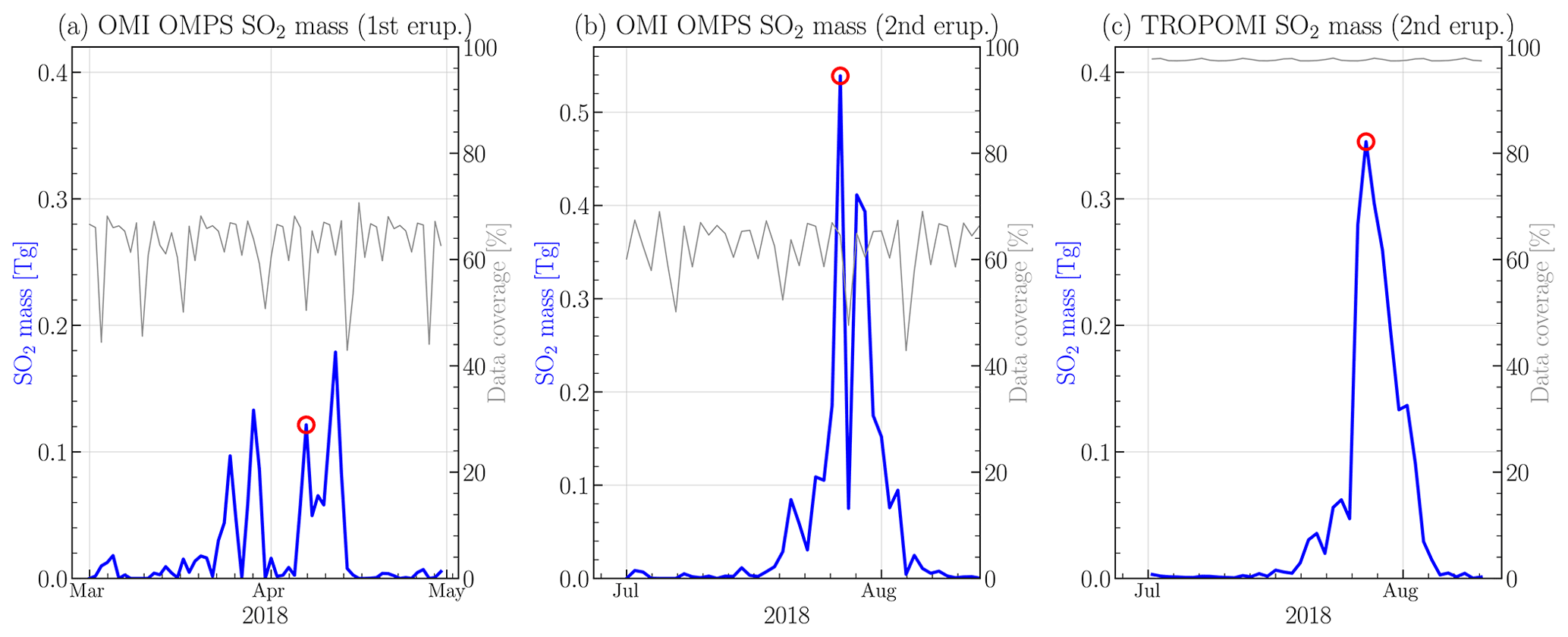
Figure C1SO2 mass for both April and July eruptions, as calculated from combined OMI/OMPS-NM data.
For transparency and to better justify the choice of TROPOMI SO2 data for the second eruption, the SO2 mass calculation for the July Ambae eruption was repeated using the OMI/OMPS-NP data set. The results were combined with those in Fig. 1 and presented in Fig. C1, where the estimated SO2 mass is plotted in blue, and the daily coverage in percent in gray. It should be noted, that the self-defined grid for the first eruption contains latitudes up to 45∘ S whereas the grid for the second eruption only reaches 35∘ S in order to be comparable with the TROPOMI analysis. Though, one should still bear in mind that, for all SO2 products, the SO2 profiles with different center mass are assumed (Sect. 3.1). For the OMI product, the SO2 center mass is located at 18 km (Sect. 3.1.1), for OMPS-NM at 16 km (Sect. 3.1.1), and for TROPOMI at 15 km (Sect. 3.1.2).
As it follows from Fig. C1b, the OMI/OMPS-NM combined product yields a maximum SO2 mass of 0.54 Tg on 27 July 2018, which is the same day as TROPOMI product (Fig. C1c). It is somewhat counterintuitive that OMI/OMPS-NM estimate gives a higher maximum SO2 mass than the one from TROPOMI (see Sect. 3.1.2), although the OMI/OMPS-NM data have large data gaps. However, at the same time, the OMI/OMPS-NM data for July appear to be noisier than TROPOMI. Calculating the averages of the SO2 mass from 26 to 29 July 2018, where the majority of the discrepancies between the two products occur, one achieves 0.32 and 0.28 Tg for the OMI/OMPS-NM and TROPOMI products, respectively. Though these averages can be considered somewhat arbitrary, they show that, independent from the data set choice, the July eruption was significantly larger than the June one, and the value of 0.36 Tg (Sect. 4.1.2) used for ECHAM simulation of the second eruption is quite robust.
OMPS-LP aerosol extinction coefficient at 869 nm data are available after registration at http://www.iup.uni-bremen.de/DataRequest/ (Malinina et al., 2019). ECHAM primary data and scripts used in the analysis and other supplementary information that may be useful in reproducing the authors' model work are archived by the Max Planck Institute for Meteorology and can be obtained by contacting publications@mpimet.mpg.de. Model results are available at https://cera-www.dkrz.de/WDCC/ui/cerasearch/entry?acronym=DKRZ_LTA_550_ds00006 (Niemeier and Malinina, 2021). OMI (Li et al., 2020) (https://doi.org/10.5067/Aura/OMI/DATA2022) and OMPS-NM (Yang, 2017) (https://doi.org/10.5067/A9O02ZH0J94R) L2 data, as well as for OMPS-LP L1 data, were obtained from the NASA Langley Research Center EOSDIS Distributed Active Archive Center. MLS and SAGE-III/ISS L2 data were obtained from Read and Livsey (2015) and NASA's Earthdata (2020b), respectively. S5P TROPOMI data were downloaded from S5P Data Hub (2020).
The supplement related to this article is available online at: https://doi.org/10.5194/acp-21-14871-2021-supplement.
EM initiated the study, provided OMPS-LP aerosol extinction coefficient product, compared it to SAGE-III/ISS, prepared the figures, and wrote most of the text (Sects. 1–2.6 and 3.2–5). AR developed the retrieval software, supervised the work at the University of Bremen, wrote part of Sect. 4.2, and revised the rest of the paper. UN performed model simulations, wrote Sects. 2.7 and 4.1.3, helped with the literature survey, and revised the text. SW performed SO2 mass estimations, wrote Sect. 3.1, provided data for Figs. 1 and B1, and revised the text. CA formatted OMPS L1 data, analyzed MLS data, provided data for Fig. A1 and tropopause heights for OMPS-LP, and revised the text. FW actively participated in the result discussions and revised the text. CT helped with literature survey. CvS and CT initiated and proposed the research unit; they and JPB led the project and revised the text.
The authors declare that they have no conflict of interest.
Publisher's note: Copernicus Publications remains neutral with regard to jurisdictional claims in published maps and institutional affiliations.
This work has been funded, in part, by the German Research Foundation (DFG) through the research unit VolImpact (FOR 2820; projects VolARC, VolDyn, and VolClim), ESA through Ozone-CCI+ project, and the University of Bremen and state of Bremen. The model simulations were performed on the computer of the Deutsches Klimarechenzentrum (DKRZ). We are also thankful to NASA for the OMI (NASA GES DISC, 2020a) and OMPS-NM (NASA GES DISC, 2020b) L2 data, as well as for OMPS-LP L1 data, which were downloaded from the NASA Langley Research Center EOSDIS Distributed Active Archive Center. MLS and SAGE-III/ISS L2 data were obtained from NASA's Earthdata (2020a) and NASA's Earthdata (2020b), respectively. S5P TROPOMI data were downloaded from S5P Data Hub (2020).
This research has been supported by the German Research Foundation (DFG; grant no. FOR 2820).
The article processing charges for this open-access publication were covered by the University of Bremen.
This paper was edited by Manvendra K. Dubey and reviewed by Daniele Visioni and one anonymous referee.
Arosio, C., Rozanov, A., Malinina, E., Eichmann, K.-U., von Clarmann, T., and Burrows, J. P.: Retrieval of ozone profiles from OMPS limb scattering observations, Atmos. Meas. Tech., 11, 2135–2149, https://doi.org/10.5194/amt-11-2135-2018, 2018. a, b
Bertaux, J., Hauchecorne, A., Dalaudier, F., Cot, C., Kyrölä, E., Fussen, D., Tamminen, J., Leppelmeier, G., Sofieva, V., Hassinen, S., Fanton d'Andon, O., Barrot, G., Mangin, A., Theodore, B., Guirlet, M., Korablev, O., Snoeij, P., Koopman, R., and Fraisse, R.: First results on GOMOS/Envisat, Adv. Space Res., 33, 1029–1035, 2004. a
Bingen, C., Fussen, D., and Vanhellemont, F.: A global climatology of stratospheric aerosol size distribution parameters derived from SAGE II data over the period 1984–2000: 1. Methodology and climatological observations, J. Geophys. Res.-Atmos., 109, 2004. a, b
Bourassa, A., Degenstein, D., Elash, B., and Llewellyn, E.: Evolution of the stratospheric aerosol enhancement following the eruptions of Okmok and Kasatochi: Odin-OSIRIS measurements, J. Geophys. Res.-Atmos., 115, D00L03, https://doi.org/10.1029/2009JD013274, 2010. a
Bourassa, A. E., Rieger, L. A., Zawada, D. J., Khaykin, S., Thomason, L., and Degenstein, D. A.: Satellite Limb Observations of Unprecedented Forest Fire Aerosol in the Stratosphere, J. Geophys. Res.-Atmos., 124, 9510–9519, https://doi.org/10.1029/2019JD030607, 2019. a, b, c
Brinkhoff, L. A., Rozanov, A., Hommel, R., von Savigny, C., Ernst, F., Bovensmann, H., and Burrows, J. P.: Ten-Year SCIAMACHY Stratospheric Aerosol Data Record: Signature of the Secondary Meridional Circulation Associated with the Quasi-Biennial Oscillation, in: Towards an Interdisciplinary Approach in Earth System Science, Springer International Publishing, Cham, 49–58, 2015. a
Brühl, C., Schallock, J., Klingmüller, K., Robert, C., Bingen, C., Clarisse, L., Heckel, A., North, P., and Rieger, L.: Stratospheric aerosol radiative forcing simulated by the chemistry climate model EMAC using Aerosol CCI satellite data, Atmos. Chem. Phys., 18, 12845–12857, https://doi.org/10.5194/acp-18-12845-2018, 2018. a
Carboni, E., Grainger, R. G., Mather, T. A., Pyle, D. M., Thomas, G. E., Siddans, R., Smith, A. J. A., Dudhia, A., Koukouli, M. E., and Balis, D.: The vertical distribution of volcanic SO2 plumes measured by IASI, Atmos. Chem. Phys., 16, 4343–4367, https://doi.org/10.5194/acp-16-4343-2016, 2016. a, b
Carn, S., Yang, K., Prata, A., and Krotkov, N.: Extending the long-term record of volcanic SO2 emissions with the Ozone Mapping and Profiler Suite nadir mapper, Geophys. Res. Lett., 42, 925–932, 2015. a
Chen, Z., DeLand, M., and Bhartia, P. K.: A new algorithm for detecting cloud height using OMPS/LP measurements, Atmos. Meas. Tech., 9, 1239–1246, https://doi.org/10.5194/amt-9-1239-2016, 2016. a
Chen, Z., Bhartia, P. K., Loughman, R., Colarco, P., and DeLand, M.: Improvement of stratospheric aerosol extinction retrieval from OMPS/LP using a new aerosol model, Atmos. Meas. Tech., 11, 6495–6509, https://doi.org/10.5194/amt-11-6495-2018, 2018. a
Chen, Z., Bhartia, P. K., Torres, O., Jaross, G., Loughman, R., DeLand, M., Colarco, P., Damadeo, R., and Taha, G.: Evaluation of the OMPS/LP stratospheric aerosol extinction product using SAGE III/ISS observations, Atmos. Meas. Tech., 13, 3471–3485, https://doi.org/10.5194/amt-13-3471-2020, 2020. a
Cisewski, M., Zawodny, J., Gasbarre, J., Eckman, R., Topiwala, N., Rodriguez-Alvarez, O., Cheek, D., and Hall, S.: The Stratospheric Aerosol and Gas Experiment (SAGE III) on the International Space Station (ISS) Mission, in: Sensors, Systems, and Next-Generation Satellites XVIII, International Society for Optics and Photonics, SPIE, 9241, 59–65, https://doi.org/10.1117/12.2073131, 2014. a, b
Clyne, M., Lamarque, J.-F., Mills, M. J., Khodri, M., Ball, W., Bekki, S., Dhomse, S. S., Lebas, N., Mann, G., Marshall, L., Niemeier, U., Poulain, V., Robock, A., Rozanov, E., Schmidt, A., Stenke, A., Sukhodolov, T., Timmreck, C., Toohey, M., Tummon, F., Zanchettin, D., Zhu, Y., and Toon, O. B.: Model physics and chemistry causing intermodel disagreement within the VolMIP-Tambora Interactive Stratospheric Aerosol ensemble, Atmos. Chem. Phys., 21, 3317–3343, https://doi.org/10.5194/acp-21-3317-2021, 2021. a
Damadeo, R. P., Zawodny, J. M., Thomason, L. W., and Iyer, N.: SAGE version 7.0 algorithm: application to SAGE II, Atmos. Meas. Tech., 6, 3539–3561, https://doi.org/10.5194/amt-6-3539-2013, 2013. a, b
Dhomse, S. S., Mann, G. W., Antuña Marrero, J. C., Shallcross, S. E., Chipperfield, M. P., Carslaw, K. S., Marshall, L., Abraham, N. L., and Johnson, C. E.: Evaluating the simulated radiative forcings, aerosol properties, and stratospheric warmings from the 1963 Mt Agung, 1982 El Chichón, and 1991 Mt Pinatubo volcanic aerosol clouds, Atmos. Chem. Phys., 20, 13627–13654, https://doi.org/10.5194/acp-20-13627-2020, 2020. a
Feinberg, A., Sukhodolov, T., Luo, B.-P., Rozanov, E., Winkel, L. H. E., Peter, T., and Stenke, A.: Improved tropospheric and stratospheric sulfur cycle in the aerosol–chemistry–climate model SOCOL-AERv2, Geosci. Model Dev., 12, 3863–3887, https://doi.org/10.5194/gmd-12-3863-2019, 2019. a
Fioletov, V., McLinden, C. A., Griffin, D., Theys, N., Loyola, D. G., Hedelt, P., Krotkov, N. A., and Li, C.: Anthropogenic and volcanic point source SO2 emissions derived from TROPOMI on board Sentinel-5 Precursor: first results, Atmos. Chem. Phys., 20, 5591–5607, https://doi.org/10.5194/acp-20-5591-2020, 2020. a, b
Fioletov, V. E., McLinden, C. A., Krotkov, N., Li, C., Joiner, J., Theys, N., Carn, S., and Moran, M. D.: A global catalogue of large SO2 sources and emissions derived from the Ozone Monitoring Instrument, Atmos. Chem. Phys., 16, 11497–11519, https://doi.org/10.5194/acp-16-11497-2016, 2016. a
Fischer, H., Birk, M., Blom, C., Carli, B., Carlotti, M., von Clarmann, T., Delbouille, L., Dudhia, A., Ehhalt, D., Endemann, M., Flaud, J. M., Gessner, R., Kleinert, A., Koopman, R., Langen, J., López-Puertas, M., Mosner, P., Nett, H., Oelhaf, H., Perron, G., Remedios, J., Ridolfi, M., Stiller, G., and Zander, R.: MIPAS: an instrument for atmospheric and climate research, Atmos. Chem. Phys., 8, 2151–2188, https://doi.org/10.5194/acp-8-2151-2008, 2008. a
Flynn, L., Long, C., Wu, X., Evans, R., Beck, C., Petropavlovskikh, I., McConville, G., Yu, W., Zhang, Z., Niu, J., Flynn, L., Long, C., Wu, X., Evans, R., Beck, C., Petropavlovskikh, I., McConville, G., Yu, W., Zhang, Z., Niu, J, Beach, E., Hao, Y., Pan, C., Sen, B., Novicki, M., Zhou, S., and Seftor, C.: Performance of the ozone mapping and profiler suite (OMPS) products, J. Geophys. Res.-Atmos., 119, 6181–6195, 2014. a
Fromm, M., Lindsey, D. T., Servranckx, R., Yue, G., Trickl, T., Sica, R., Doucet, P., and Godin-Beekmann, S.: The untold story of pyrocumulonimbus, B. Am. Meteorol. Soc., 91, 1193–1210, 2010. a
Fussen, D. and Bingen, C.: Volcanism dependent model for the extinction profile of stratospheric aerosols in the UV-visible range, Geophys. Res. Lett., 26, 703–706, 1999. a
Giorgetta, M. A., Manzini, E., Roeckner, E., Esch, M., and Bengtsson, L.: Climatology and forcing of the quasi–biennial oscillation in the MAECHAM5 model, J. Climate, 19, 3882–3901, 2006. a
Gottwald, M. and Bovensmann, H.: SCIAMACHY – Exploring the Changing Earth's Atmosphere, Springer, Dordrecht, https://doi.org/10.1007/978-90-481-9896-2, 2011. a
Hansen, J., Sato, M., Ruedy, R., Nazarenko, L., Lacis, A., Schmidt, G., Russell, G., Aleinov, I., Bauer, M., Bauer, S., Bell, N., Cairns, B., Canuto, V., Chandler, M., Cheng, Y., Del Genio, A., Faluvegi, G., Fleming, E., Friend, A., Hall, T., Jackman, C., Kelley, M., Kiang, N., Koch, D., Lean, J., Lerner, J., Lo, K., Menon, S., Miller, R., Minnis, P., Novakov, T., Oinas, V., Perlwitz, J., Perlwitz, J., Rind, D., Romanou, A., Shindell, D., Stone, P., Sun, S., Tausnev, N., Thresher, D., Wielicki, B., Wong, T., Yao, M., and Zhang, S.: Efficacy of climate forcings, J. Geophys. Res.-Atmos., 110, D18104, https://doi.org/10.1029/2005JD005776, 2005. a
Haywood, J. M., Jones, A., Clarisse, L., Bourassa, A., Barnes, J., Telford, P., Bellouin, N., Boucher, O., Agnew, P., Clerbaux, C., Coheur, P., Degenstein, D., and Braesicke, P.: Observations of the eruption of the Sarychev volcano and simulations using the HadGEM2 climate model, J. Geophys. Res.-Atmos., 115, D21212, https://doi.org/10.1029/2010JD014447, 2010. a, b
Haywood, J. M., Jones, A., and Jones, G. S.: The impact of volcanic eruptions in the period 2000–2013 on global mean temperature trends evaluated in the HadGEM2-ES climate model, Atmos. Sci. Lett., 15, 92–96, 2014. a
Hersbach, H., de Rosnay, P., Bell, B., Schepers, D., Simmons, A., Soci, C., Abdalla, S., Alonso-Balmaseda, M., Balsamo, G., Bechtold, P., Berrisford, P., Bidlot, J.-R., de Boisséson, E., Bonavita, M., Browne, P., Buizza, R., Dahlgren, P., Dee, D., Dragani, R., Diamantakis, M., Flemming, J., Forbes, R., Geer, A. J., Haiden, T., Hólm, E., Haimberger, L., Hogan, R., Horányi, A., Janiskova, M., Laloyaux, P., Lopez, P., Munoz-Sabater, J., Peubey, C., Radu, R., Richardson, D., Thépaut, J.-N., Vitart, F., Yang, X., Zsótér, E., and Zuo, H.: Operational global reanalysis: progress, future directions and synergies with NWP, ERA Report Series, ECMWF, Shinfield Park, 2018. a
Hess, M., Koepke, P., and Schult, I.: Optical properties of aerosols and clouds: The software package OPAC, B. Am. Meteorol. Soc., 79, 831–844, 1998. a
Hitchman, M. H., McKay, M., and Trepte, C. R.: A climatology of stratospheric aerosol, J. Geophys. Res.-Atmos., 99, 20689–20700, 1994. a
Hommel, R., Timmreck, C., and Graf, H. F.: The global middle-atmosphere aerosol model MAECHAM5-SAM2: comparison with satellite and in-situ observations, Geosci. Model Dev., 4, 809–834, https://doi.org/10.5194/gmd-4-809-2011, 2011. a
Hommel, R., Timmreck, C., Giorgetta, M. A., and Graf, H. F.: Quasi-biennial oscillation of the tropical stratospheric aerosol layer, Atmos. Chem. Phys., 15, 5557–5584, https://doi.org/10.5194/acp-15-5557-2015, 2015. a
Hurrell, J. W., Hack, J. J., Shea, D., Caron, J. M., and Rosinski, J.: A New Sea Surface Temperature and Sea Ice Boundary Dataset for the Community Atmosphere Model, J. Climate, 21, 5145–5153, https://doi.org/10.1175/2008JCLI2292.1, 2008. a
Ivy, D. J., Solomon, S., Kinnison, D., Mills, M. J., Schmidt, A., and Neely, R. R.: The influence of the Calbuco eruption on the 2015 Antarctic ozone hole in a fully coupled chemistry-climate model, Geophys. Res. Lett., 44, 2556–2561, 2017. a
Jaross, G., Bhartia, P. K., Chen, G., Kowitt, M., Haken, M., Chen, Z., Xu, P., Warner, J., and Kelly, T.: OMPS Limb Profiler instrument performance assessment, J. Geophys. Res.-Atmos., 119, 4399–4412, https://doi.org/10.1002/2013JD020482, 2014. a, b
Kang, M.-J. and Chun, H.-Y.: Contributions of equatorial waves and small-scale convective gravity waves to the 2019/20 quasi-biennial oscillation (QBO) disruption, Atmos. Chem. Phys., 21, 9839–9857, https://doi.org/10.5194/acp-21-9839-2021, 2021. a
Khaykin, S., Godin-Beekmann, S., Hauchecorne, A., Pelon, J., Ravetta, F., and Keckhut, P.: Stratospheric smoke with unprecedentedly high backscatter observed by lidars above southern France, Geophys. Res. Lett., 45, 1639–1646, 2018. a
Khaykin, S., Legras, B., Bucci, S., Sellitto, P., Isaksen, L., Tence, F., Bekki, S., Bourassa, A., Rieger, L., Zawada, D., Jumelet, J., and Godin-Beekmann, S.: The 2019/20 Australian wildfires generated a persistent smoke-charged vortex rising up to 35 km altitude, Communications Earth & Environment, 1, 1–12, 2020. a
Kloss, C., Berthet, G., Sellitto, P., Ploeger, F., Bucci, S., Khaykin, S., Jégou, F., Taha, G., Thomason, L. W., Barret, B., Le Flochmoen, E., von Hobe, M., Bossolasco, A., Bègue, N., and Legras, B.: Transport of the 2017 Canadian wildfire plume to the tropics via the Asian monsoon circulation, Atmos. Chem. Phys., 19, 13547–13567, https://doi.org/10.5194/acp-19-13547-2019, 2019. a
Kloss, C., Sellitto, P., Legras, B., Vernier, J.-P., Jégou, F., Venkat Ratnam, M., Kumar, B. S., Madhavan, B. L., and Berthet, G.: Impact of the 2018 Ambae eruption on the global stratospheric aerosol layer and climate, J. Geophys. Res.-Atmos., 125, e2020JD032410, https://doi.org/10.1029/2020JD032410, 2020. a, b, c, d, e, f, g, h
Kravitz, B., Robock, A., and Bourassa, A.: Negligible climatic effects from the 2008 Okmok and Kasatochi volcanic eruptions, J. Geophys. Res.-Atmos., 115, D00L05, https://doi.org/10.1029/2009JD013525, 2010. a, b
Kravitz, B., Robock, A., Bourassa, A., Deshler, T., Wu, D., Mattis, I., Finger, F., Hoffmann, A., Ritter, C., Bitar, L., Duck, T. J., and Barne, J. E.: Simulation and observations of stratospheric aerosols from the 2009 Sarychev volcaniceruption, J. Geophys. Res., 116, D18211, https://doi.org/10.1029/2010JD015501, 2011. a, b
Kremser, S., Thomason, L. W., Hobe, M., Hermann, M., Deshler, T., Timmreck, C., Toohey, M., Stenke, A., Schwarz, J. P., Weigel, R., Fueglistaler, S., Prata, F. J., Vernier, J.-P., Schlager, H., Barnes, J. E., Antu na-Marrero, J.-C., Fairlie, D., Palm, M., Mahieu, E., Notholt, J., Rex, M., Bingen, C., Vanhellemont, F., Bourassa, A., Plane, J. M. C., Klocke, D., Carn, S. A., Clarisse, L., Trickl, T., Neely, R., James, A. D., Rieger, L., Wilson, J. C., and Meland, B.: Stratospheric aerosol–Observations, processes, and impact on climate, Rev. Geophys., 54, 278–335, https://doi.org/10.1002/2015RG000511, 2016. a, b, c
Levelt, P., van den Oord, G., Dobber, M., Malkki, A., Visser, H., de Vries, J., Stammes, P., Lundell, J., and Saari, H.: The ozone monitoring instrument, IEEE T. Geosci. Remote, 44, 1093–1101, https://doi.org/10.1109/TGRS.2006.872333, 2006. a
Levelt, P. F., Joiner, J., Tamminen, J., Veefkind, J. P., Bhartia, P. K., Stein Zweers, D. C., Duncan, B. N., Streets, D. G., Eskes, H., van der A, R., McLinden, C., Fioletov, V., Carn, S., de Laat, J., DeLand, M., Marchenko, S., McPeters, R., Ziemke, J., Fu, D., Liu, X., Pickering, K., Apituley, A., González Abad, G., Arola, A., Boersma, F., Chan Miller, C., Chance, K., de Graaf, M., Hakkarainen, J., Hassinen, S., Ialongo, I., Kleipool, Q., Krotkov, N., Li, C., Lamsal, L., Newman, P., Nowlan, C., Suleiman, R., Tilstra, L. G., Torres, O., Wang, H., and Wargan, K.: The Ozone Monitoring Instrument: overview of 14 years in space, Atmos. Chem. Phys., 18, 5699–5745, https://doi.org/10.5194/acp-18-5699-2018, 2018. a, b
Li, C., Krotkov, N. A., Carn, S., Zhang, Y., Spurr, R. J. D., and Joiner, J.: New-generation NASA Aura Ozone Monitoring Instrument (OMI) volcanic SO2 dataset: algorithm description, initial results, and continuation with the Suomi-NPP Ozone Mapping and Profiler Suite (OMPS), Atmos. Meas. Tech., 10, 445–458, https://doi.org/10.5194/amt-10-445-2017, 2017. a
Li, C., Krotkov, N. A., Leonard, P., and Joiner, J.: OMI/Aura Sulphur Dioxide (SO2) Total Column 1-orbit L2 Swath 13×24 km V003, Greenbelt, MD, USA, GES DISC – Goddard Earth Sciences Data and Information Services Center [data set], https://doi.org/10.5067/Aura/OMI/DATA2022, 2020. a
Llewellyn, E., Lloyd, N., Degenstein, D., Gattinger, R., Petelina, S., Bourassa, A., Wiensz, J., Ivanov, E., McDade, I., Solheim, B., McConnell, J. C., Haley, C. S., von Savigny, C., Sioris, C. E., McLinden, C. A., Griffioen, E., Kaminski, J., Evans, W. F. J., Puckrin, E., Strong, K., Wehrle, V., Hum, R. H., Kendall, D. J. W., Matsushita, J., Murtagh, D. P., Brohede, S., Stegman, J., Witt, G., Barnes, G., Payne, W. F., Piché, L., Smith, K., Warshaw, G., Deslauniers, D.-L., Marchand, P., Richardson, E. H., King, R. A., Wevers, I., McCreath, W., Kyrölä, E., Oikarinen, L., Leppelmeier, G. W., Auvinen, H., Mégie, G., Hauchecorne, A., Lefèvre, F., de La Nöe, J., Ricaud, P., Frisk, U., Sjoberg, F., von Schéele, F., and Nordh, L.: The OSIRIS instrument on the Odin spacecraft, Can. J. Phys., 82, 411–422, 2004. a
Loughman, R., Bhartia, P. K., Chen, Z., Xu, P., Nyaku, E., and Taha, G.: The Ozone Mapping and Profiler Suite (OMPS) Limb Profiler (LP) Version 1 aerosol extinction retrieval algorithm: theoretical basis, Atmos. Meas. Tech., 11, 2633–2651, https://doi.org/10.5194/amt-11-2633-2018, 2018. a
Lurton, T., Jégou, F., Berthet, G., Renard, J.-B., Clarisse, L., Schmidt, A., Brogniez, C., and Roberts, T. J.: Model simulations of the chemical and aerosol microphysical evolution of the Sarychev Peak 2009 eruption cloud compared to in situ and satellite observations, Atmos. Chem. Phys., 18, 3223–3247, https://doi.org/10.5194/acp-18-3223-2018, 2018. a, b
Maddox, E. M. and Mullendore, G. L.: Determination of best tropopause definition for convective transport studies, J. Atmos. Sci., 75, 3433–3446, 2018. a
Malinina, E.: Retrieval of stratospheric aerosol characteristics from spaceborne limb sounders, PhD thesis, University of Bremen, available at: http://nbn-resolving.de/urn:nbn:de:gbv:46-00107153-12 (last access: 29 September 2021), 2019. a, b, c, d, e
Malinina, E., Rozanov, A., Rozanov, V., Liebing, P., Bovensmann, H., and Burrows, J. P.: Aerosol particle size distribution in the stratosphere retrieved from SCIAMACHY limb measurements, Atmos. Meas. Tech., 11, 2085–2100, https://doi.org/10.5194/amt-11-2085-2018, 2018. a, b
Malinina, E., Rozanov, A., and Arosio, C.: IUP Stratospheric Aerosol Extinction from OMPS-LP, available at: http://www.iup.uni-bremen.de/DataRequest/, last access: 29 September 2019. a
Marshall, L., Schmidt, A., Toohey, M., Carslaw, K. S., Mann, G. W., Sigl, M., Khodri, M., Timmreck, C., Zanchettin, D., Ball, W. T., Bekki, S., Brooke, J. S. A., Dhomse, S., Johnson, C., Lamarque, J.-F., LeGrande, A. N., Mills, M. J., Niemeier, U., Pope, J. O., Poulain, V., Robock, A., Rozanov, E., Stenke, A., Sukhodolov, T., Tilmes, S., Tsigaridis, K., and Tummon, F.: Multi-model comparison of the volcanic sulfate deposition from the 1815 eruption of Mt. Tambora, Atmos. Chem. Phys., 18, 2307–2328, https://doi.org/10.5194/acp-18-2307-2018, 2018. a
McCormick, M. P., Lei, L., Hill, M. T., Anderson, J., Querel, R., and Steinbrecht, W.: Early results and validation of SAGE III-ISS ozone profile measurements from onboard the International Space Station, Atmos. Meas. Tech., 13, 1287–1297, https://doi.org/10.5194/amt-13-1287-2020, 2020. a
Mettig, N., Weber, M., Rozanov, A., Arosio, C., Burrows, J. P., Veefkind, P., Thompson, A. M., Querel, R., Leblanc, T., Godin-Beekmann, S., Kivi, R., and Tully, M. B.: Ozone Profile Retrieval from nadir TROPOMI measurements in the UV range, Atmos. Meas. Tech. Discuss. [preprint], https://doi.org/10.5194/amt-2021-32, in review, 2021. a
Mills, M. J., Richter, J. H., Tilmes, S., Kravitz, B., MacMartin, D. G., Glanville, A. A., Tribbia, J. J., Lamarque, J.-F., Vitt, F., Schmidt, A., Gettelman, A., Hannay, C., Bacmeister, J. T., and Kinnison, D. E.: Radiative and Chemical Response to Interactive Stratospheric Sulfate Aerosols in Fully Coupled CESM1(WACCM), J. Geophys. Res.-Atmos., 122, 13061–13078, https://doi.org/10.1002/2017JD027006, 2017. a
Moussallam, Y., Rose-Koga, E. F., Koga, K. T., Médard, E., Bani, P., Devidal, J.-L., and Tari, D.: Fast ascent rate during the 2017–2018 Plinian eruption of Ambae (Aoba) volcano: a petrological investigation, Contrib. Mineral. Petr., 174, 90, https://doi.org/10.1007/s00410-019-1625-z, 2019. a, b, c
Muser, L. O., Hoshyaripour, G. A., Bruckert, J., Horváth, Á., Malinina, E., Wallis, S., Prata, F. J., Rozanov, A., von Savigny, C., Vogel, H., and Vogel, B.: Particle aging and aerosol–radiation interaction affect volcanic plume dispersion: evidence from the Raikoke 2019 eruption, Atmos. Chem. Phys., 20, 15015–15036, https://doi.org/10.5194/acp-20-15015-2020, 2020. a
NASA GES DISC: OMSO2: OMI/Aura Sulphur Dioxide (SO2) Total Column 1-orbit L2 Swath 13 × 24 km V003 [data set], available at: https://disc.gsfc.nasa.gov/datasets/OMSO2_003/summary (last access: 29 September 2021), 2020a. a
NASA GES DISC: OMPS_NPP_NMSO2_L2: OMPS-NPP L2 NM Sulfur Dioxide (SO2) Total and Tropospheric Column swath orbital V2, available at: https://disc.gsfc.nasa.gov/datasets/OMPS_NPP_NMSO2_L2_2/summary (last access: 29 September 2021), 2020b. a
NASA GES DISC: OMPS_NPP_Products, available at: https://disc.gsfc.nasa.gov/datasets?keywords=omps&page=1&source=SUOMI-NPP%20OMPS (last access: 29 September 2021), 2021. a
NASA's Earthdata: MLS/Aura Level 2 Sulfur Dioxide (SO2) Mixing Ratio V004 (ML2SO2) at GES DISC [data set], available at: https://search.earthdata.nasa.gov/search?p=C1251101777-GES_DISC&q=ML2SO2_004 (last access: 29 September 2021), 2020a. a
NASA's Earthdata: SAGE III/ISS L2 Solar Event Species Profiles (HDF-EOS) V051 [data set], available at: https://search.earthdata.nasa.gov/search/granules?p=C1576312558-LARC&fpj=SAGE%20III/ISS&tl=1574370747!4!! (last access: 29 September 2021), 2020b. a, b
Newman, P., Coy, L., Pawson, S., and Lait, L.: The anomalous change in the QBO in 2015–2016, Geophys. Res. Lett., 43, 8791–8797, 2016. a
Niemeier, U. and Malinina, E.: ECHAM-HAM data for: Changes in stratospheric aerosol extinction coefficient after the 2018 Ambae eruption as seen by OMPS-LP and ECHAM5-HAM, World Data Center for Climate (WDCC) at DKRZ [data set], available at: http://cera-www.dkrz.de/WDCC/ui/Compact.jsp?acronym=DKRZ_LTA_550_ds00006, last access: 4 October 2021. a
Niemeier, U. and Timmreck, C.: What is the limit of climate engineering by stratospheric injection of SO2?, Atmos. Chem. Phys., 15, 9129–9141, https://doi.org/10.5194/acp-15-9129-2015, 2015. a
Niemeier, U., Timmreck, C., Graf, H.-F., Kinne, S., Rast, S., and Self, S.: Initial fate of fine ash and sulfur from large volcanic eruptions, Atmos. Chem. Phys., 9, 9043–9057, https://doi.org/10.5194/acp-9-9043-2009, 2009. a, b, c
Oman, L., Robock, A., Stenchikov, G. L., Thordarson, T., Koch, D., Shindell, D. T., and Gao, C.: Modeling the distribution of the volcanic aerosol cloud from the 1783–1784 Laki eruption, J. Geophys. Res.-Atmos., 111, D12209, https://doi.org/10.1029/2005JD006899, 2006. a
Pitari, G., Visioni, D., Mancini, E., Cionni, I., Di Genova, G., and Gandolfi, I.: Sulfate aerosols from non-explosive volcanoes: chemical-radiative effects in the troposphere and lower stratosphere, Atmosphere, 7, 85, https://doi.org/10.3390/atmos7070085, 2016. a
Pumphrey, H. C., Read, W. G., Livesey, N. J., and Yang, K.: Observations of volcanic SO2 from MLS on Aura, Atmos. Meas. Tech., 8, 195–209, https://doi.org/10.5194/amt-8-195-2015, 2015. a
Randel, W. J., Park, M., Emmons, L., Kinnison, D., Bernath, P., Walker, K. A., Boone, C., and Pumphrey, H.: Asian monsoon transport of pollution to the stratosphere, Science, 328, 611–613, 2010. a
Read, W. and Livesey, N.: MLS/Aura Level 2 Sulfur Dioxide (SO2) Mixing Ratio V004, GES DISC – Goddard Earth Sciences Data and Information Services Center [data set], https://doi.org/10.5067/Aura/MLS/DATA2020, 2015. a
Rieger, L., Zawada, D., Bourassa, A., and Degenstein, D.: A multiwavelength retrieval approach for improved OSIRIS aerosol extinction retrievals, J. Geophys. Res.-Atmos., 124, 7286–7307, 2019. a
Rieger, L. A., Malinina, E. P., Rozanov, A. V., Burrows, J. P., Bourassa, A. E., and Degenstein, D. A.: A study of the approaches used to retrieve aerosol extinction, as applied to limb observations made by OSIRIS and SCIAMACHY, Atmos. Meas. Tech., 11, 3433–3445, https://doi.org/10.5194/amt-11-3433-2018, 2018. a, b, c, d, e, f
Schmidt, A., Mills, M. J., Ghan, S., Gregory, J. M., Allan, R. P., Andrews, T., Bardeen, C. G., Conley, A., Forster, P. M., Gettelman, A., Portmann, R. W., Solomon, S., and Toon, O. B.: Volcanic radiative forcing from 1979 to 2015, J. Geophys. Res.-Atmos., 123, 12491–12508, 2018. a
Seftor, C., Jaross, G., Kowitt, M., Haken, M., Li, J., and Flynn, L.: Postlaunch performance of the Suomi National Polar-orbiting Partnership Ozone Mapping and Profiler Suite (OMPS) nadir sensors, J. Geophys. Res.-Atmos., 119, 4413–4428, 2014. a
S5P Data Hub: Sentinel-P Pre-Operations Data Hub [data set], available at: https://s5phub.copernicus.eu/dhus/#/home (last access: 29 September 2021), 2020. a, b
Siddaway, J. and Petelina, S.: Transport and evolution of the 2009 Australian Black Saturday bushfire smoke in the lower stratosphere observed by OSIRIS on Odin, J. Geophys. Res.-Atmos., 116, D06203, https://doi.org/10.1029/2010JD015162, 2011. a, b
Smithsonian Institution: Global Volcanism Program Database, available at: http://volcano.si.edu/search_eruption.cfm (last access: 29 September 2021), 2019. a, b
Solomon, S.: Stratospheric ozone depletion: A review of concepts and history, Rev. Geophys., 37, 275–316, 1999. a
Solomon, S., Daniel, J. S., Neely, R. R., Vernier, J.-P., Dutton, E. G., and Thomason, L. W.: The persistently variable “background” stratospheric aerosol layer and global climate change, Science, 333, 866–870, 2011. a, b
Stier, P., Feichter, J., Kinne, S., Kloster, S., Vignati, E., Wilson, J., Ganzeveld, L., Tegen, I., Werner, M., Balkanski, Y., Schulz, M., Boucher, O., Minikin, A., and Petzold, A.: The aerosol-climate model ECHAM5-HAM, Atmos. Chem. Phys., 5, 1125–1156, https://doi.org/10.5194/acp-5-1125-2005, 2005. a
Theys, N., De Smedt, I., Yu, H., Danckaert, T., van Gent, J., Hörmann, C., Wagner, T., Hedelt, P., Bauer, H., Romahn, F., Pedergnana, M., Loyola, D., and Van Roozendael, M.: Sulfur dioxide retrievals from TROPOMI onboard Sentinel-5 Precursor: algorithm theoretical basis, Atmos. Meas. Tech., 10, 119–153, https://doi.org/10.5194/amt-10-119-2017, 2017. a, b
Theys, N., Romahn, F., and Wagner, T.: S5P Mission Performance Centre Sulphur Dioxide Readme, s5P-MPC-BIRA-PRF-SO2, V02.01.04, available at: https://sentinel.esa.int/documents/247904/3541451/Sentinel-5P-Sulphur-Dioxide-Readme.pdf (last access: 29 September 2021), 2020. a
Thomason, L. and Peter, T.: SPARC Assessment of Stratospheric Aerosol Properties (ASAP), Tech. rep., SPARC, available at: http://www.sparc-climate.org/publications/sparc-reports/ (last access: 29 September 2021), 2006. a
Timmreck, C.: Three–dimensional simulation of stratospheric background aerosol: First results of a multiannual general circulation model simulation, J. Geophys. Res., 106, 28313–28332, 2001. a
Toohey, M., Krüger, K., Schmidt, H., Timmreck, C., Sigl, M., Stoffel, M., and Wilson, R.: Disproportionately strong climate forcing from extratropical explosive volcanic eruptions, Nat. Geosci., 12, 100–107, 2019. a
Veefkind, J., Aben, I., McMullan, K., Förster, H., de Vries, J., Otter, G., Claas, J., Eskes, H., de Haan, J., Kleipool, Q., van Weele, M.,Hasekamp, O., Hoogeveen, R., Landgraf, J., Snel, R., Tol, P., Ingmann, P., Voors, R., Kruizinga, B., Vink, R., Visser, H., and Levelt, P.: TROPOMI on the ESA Sentinel-5 Precursor: A GMES mission for global observations of the atmospheric composition for climate, air quality and ozone layer applications, Remote Sens. Environ., 120, 70–83, 2012. a, b
Vernier, J.-P., Thomason, L., and Kar, J.: CALIPSO detection of an Asian tropopause aerosol layer, Geophys. Res. Lett., 38, L07804, https://doi.org/10.1029/2010GL046614, 2011. a, b, c
von Savigny, C., Ernst, F., Rozanov, A., Hommel, R., Eichmann, K.-U., Rozanov, V., Burrows, J. P., and Thomason, L. W.: Improved stratospheric aerosol extinction profiles from SCIAMACHY: validation and sample results, Atmos. Meas. Tech., 8, 5223–5235, https://doi.org/10.5194/amt-8-5223-2015, 2015. a, b, c, d
von Savigny, C., Timmreck, C., Buehler, S., Burrows, J., Giorgetta, M., Hegerl, G., Horvath, A., Hoshyaripour, G. A., Hoose, C., Quaas, J., Malinina, E., Rozanov, A., Schmidt, H., Thomason, L., Toohey, M., and Vogel, B.: The Research Unit VolImpact: Revisiting the volcanic impact on atmosphere and climate – preparations for the next big volcanic eruption, Meteorol. Z., 29, 3–18, https://doi.org/10.1127/metz/2019/0999, 2020. a
Waters, J., Froidevaux, L., Harwood, R., Jarnot, R., Pickett, H., Read, W., Siegel, P., Cofield, R., Filipiak, M., Flower, D., Holden, J., Lau, G., Livesey, N., Manney, G., Pumphrey, H., Santee, M., Wu, D., Cuddy, D., Lay, R., Loo, M., Perun, V., Schwartz, M., Stek, P., Thurstans, R., Boyles, M., Chandra, K., Chavez, M., Chen, G.-S., Chudasama, B., Dodge, R., Fuller, R., Girard, M., Jiang, J., Jiang, Y., Knosp, B., LaBelle, R., Lam, J., Lee, K., Miller, D., Oswald, J., Patel, N., Pukala, D., Quintero, O., Scaff, D., Van Snyder, W., Tope, M., Wagner, P., and Walch, M.: The Earth observing system microwave limb sounder (EOS MLS) on the aura Satellite, IEEE T. Geosci. Remote, 44, 1075–1092, https://doi.org/10.1109/TGRS.2006.873771, 2006. a, b
WMO: A three-dimensional science: Second session of the commission for aerology, WMO Bulletin, 4, 134–138, 1957. a
WMO: Polar Stratospheric Ozone: Past, Present, and Future, in: Chapter 4 in WMO Scientific Assessment of Ozone Depletion (2018), UNEP/WMO Scientific Assessment of Ozone Depletion: 2018 (Report), 58, available at: https://elib.dlr.de/135115/1/Chapter4_2018OzoneAssessment.pdf (last access: 29 September 2021), 2018. a
Yang, K.: OMPS-NPP L2 NM Sulfur Dioxide (SO2) Total and Tropospheric Column swath orbital V2, Greenbelt, MD, USA, GES DISC – Goddard Earth Sciences Data and Information Services Center [data set], https://doi.org/10.5067/A9O02ZH0J94R, 2017. a
Yang, K., Carn, S. A., Ge, C., Wang, J., and Dickerson, R. R.: Advancing measurements of tropospheric NO2 from space: New algorithm and first global results from OMPS, Geophys. Res. Lett., 41, 4777–4786, 2014. a
Zhang, Y., Li, C., Krotkov, N. A., Joiner, J., Fioletov, V., and McLinden, C.: Continuation of long-term global SO2 pollution monitoring from OMI to OMPS, Atmos. Meas. Tech., 10, 1495–1509, https://doi.org/10.5194/amt-10-1495-2017, 2017. a
Zhu, Y., Toon, O. B., Kinnison, D., Harvey, V. L., Mills, M. J., Bardeen, C. G., Pitts, M., Bègue, N., Renard, J.-B., Berthet, G., and Jégou, F.: Stratospheric aerosols, polar stratospheric clouds, and polar ozone depletion after the Mount Calbuco eruption in 2015, J. Geophys. Res.-Atmos., 123, 12308–12331, https://doi.org/10.1029/2018JD028974, 2018. a
- Abstract
- Introduction
- Instruments and model
- Observational data
- Ambae eruption
- Conclusions
- Appendix A: Estimation of SO2 injection height
- Appendix B: Impact of the assumed SO2 profile on the SO2 mass estimate
- Appendix C: Estimation of SO2 burden from OMI/OMPS-NM for the second eruption
- Code and data availability
- Author contributions
- Competing interests
- Disclaimer
- Acknowledgements
- Financial support
- Review statement
- References
- Supplement