the Creative Commons Attribution 4.0 License.
the Creative Commons Attribution 4.0 License.
 | 06 Oct 2021
Trifluoroacetic acid deposition from emissions of HFO-1234yf in India, China, and the Middle East
Mary Barth
Lena Höglund-Isaksson
Pallav Purohit
Guus J. M. Velders
Sam Glaser
A. R. Ravishankara
We have investigated trifluoroacetic acid (TFA) formation from emissions of HFO-1234yf (CF3CFH2), its dry and wet deposition, and rainwater concentration over India, China, and the Middle East with GEOS-Chem and WRF-Chem models. We estimated the TFA deposition and rainwater concentrations between 2020 and 2040 for four previously published HFO-1234yf emission scenarios to bound the possible levels of TFA. We evaluated the capability of GEOS-Chem to capture the wet deposition process by comparing calculated sulfate in rainwater with observations. Our calculated TFA amounts over the USA, Europe, and China were comparable to those previously reported when normalized to the same emission. A significant proportion of TFA was found to be deposited outside the emission regions. The mean and the extremes of TFA rainwater concentrations calculated for the four emission scenarios from GEOS-Chem and WRF-Chem were orders of magnitude below the no observable effect concentration. The ecological and human health impacts now, and the continued use of HFO-1234yf in India, China, and the Middle East, are estimated to be insignificant based on the current understanding, as summarized by Neale et al. (2021).
- Article
(6093 KB) - Full-text XML
-
Supplement
(3055 KB) - BibTeX
- EndNote


The expected concentrations of trifluoroacetic acid (TFA) from the degradation of HFO-1234yf (CF3CF=CH2) emitted now and in the future by India, China, and the Middle East were calculated using GEOS-Chem and WRF-Chem models.
We conclude that, with the current knowledge of the effects of TFA on humans and ecosystems, the projected emissions through 2040 would not be detrimental.
We carried out various tests and conclude that the model results are robust.
The major uncertainty in the knowledge of the TFA concentrations and their spatial distributions is due to uncertainties in the future projected emissions.
The use of olefinic hydrofluorocarbons (HFCs) as substitutes for HFC-134a (1,1,1,2-tetrafluoroethane; CF3CFH2) are increasing in both the developed and developing countries (Velders et al., 2009). HFC-134a is a replacement for chlorofluorocarbons (CFCs) and hydrochlorofluorocarbons (HCFCs), which were phased out under the Montreal Protocol and its many amendments and adjustments (WMO/UNEP, 2007). HFC-134a is a potent greenhouse gas with a 100-year global warming potential (GWP) of 1600 (Hodnebrog et al., 2020). HFO-1234yf (2,3,3,3-tetrafluoropropene; CF3CF=CH2), with a 100-year GWP of <1 (IPCC report; Myhre et al., 2013), is a replacement for HFC-134a in automobile air conditioners (MAC; Papadimitriou et al., 2008). The atmospheric degradation of HFO-1234yf leads to trifluoro acetyl fluoride (CF3C(O)F; Young and Mabury, 2010). CF3C(O)F hydrolyzes rapidly to yield trifluoroacetic acid (TFA; CF3-C(O)OH), which is removed from the atmosphere by dry and wet deposition (George et al., 1994). The chemical lifetime of HFC-134a (∼ 14 years) is such that it is reasonably well mixed globally upon emission into the atmosphere. Therefore, its degradation and the TFA formed will occur across the globe. Only about 30 % of the emitted HFC-134a leads to TFA (Kotamarthi et al., 1998). Other research (Wallington et al., 1996) shows that hot (vibrationally excited) CF3CFHO formed in the degradation scheme would significantly reduce the TFA yield from HFC-134a. This reduction is not explicitly considered here, but we acknowledge that the noted TFA yields from HFC-134a can be viewed as upper limits. A large fraction of the formed TFA is deposited into the oceans. The fraction of HFC-134a degraded per year from 1 year's emission would be small, leading to small TFA in rainwater concentrations at a given location. However, as HFC-134a accumulates in the atmosphere, more TFA would be produced. HFO-1234yf has a shorter chemical lifetime of a few (∼ 10) days (Myhre et al., 2013), and its degradation leads almost exclusively (∼ 100 %) to CF3C(O)F. Therefore, TFA deposition per year of emission will be higher, depending on the year, and more localized spatially.
Previous studies have focused on TFA formation from emissions of either HFC-134a at the current or previous levels (Kanakidou et al., 1995; Kotamarthi et al., 1998) or HFO-1234yf substituted for current levels of HFC-134a usage (Luecken et al., 2010); then, they have mostly scaled it for scenarios of HFO-1234yf emissions in the future over the continental USA and Europe (Henne et al., 2012; Papasavva et al., 2009). Some works have distinguished between uses of HFC-134a in MAC versus total usage, while others have evaluated maximum use scenarios. These studies suggest that toxic levels of TFA in water bodies are not produced over Europe, North America, or China if HFO-1234yf replaces all the current use of HFC-134a (Henne et al., 2012; Kazil et al., 2014; Luecken et al., 2010; Wang et al., 2018). Russell et al. (2012) conducted a model study to determine TFA concentration in terminal water bodies in the contiguous USA, with TFA deposition rates from Luecken et al. (2010). They found that, after 50 years of continuous emissions, aquatic concentrations of 1 to 15 µg L−1 are projected, with extreme concentrations of up to 50 to 200 µg L−1 in the arid southwestern USA.
Kazil et al. (2014) investigated, using the WRF-Chem model, the atmospheric turnover time of HFO-1234yf, the dry and wet deposition of TFA, and the TFA rainwater concentration over the contiguous USA between May and September 2006. They also examined where TFA deposited emissions of three specific regions in the USA. They concluded that the average TFA rainwater concentration was 0.89 µg L−1 for the contiguous USA. Although Kazil et al. (2014) used emissions twice as large as those used by Luecken et al. (2010), the TFA rainwater concentrations were comparable. Kazil et al. (2014) used the measured HFC-134a to CO ratio from the Los Angeles area to obtain potential HFO-1234yf emissions. They also showed that TFA rainwater concentrations reached significantly higher values (7.8 µg L−1) at locations with very low precipitation on shorter timescales. A comparably low TFA wet deposition occurred in the dry western USA. The work of Wang et al. (2018) is similar to that of Henne et al. (2012) and used the GEOS-Chem model and examined the rainwater content and deposited amounts of TFA over Europe, the USA, and China with similar findings. Henne et al. (2012) is the only study that used two different models (FLEXPART and STOCHEM) to study the TFA deposition and rainwater concentration over Europe.
The above-noted studies focused on the USA and Europe and, most recently, China. The emissions of the sum of HFC-134a and HFO-1234yf in the USA and Europe are expected to increase only in proportion to the population in the future since the per capita number of MAC, stationary AC, and other cooling units are unlikely to increase rapidly. India, China, and the Middle East are the regions with expected large increases in HFO-1234yf use. In these regions, the number of units and associated usage will increase rapidly as the economies grow. Perhaps Latin America and parts of Africa will also see similar increases. The above-noted studies from the USA and Europe do not allow us to draw firm conclusions about TFA's formation from realistic future emissions from Asia (i.e., China and the Indian subcontinent), where the markets are not saturated, and meteorology is very different from North America and Europe. The rate of degradation of parent compounds and precipitation will differ in the warmer tropical and subtropical regions from those seen for the USA and Europe; the seasonality will also be different. The precipitation across Asia is associated with the Asian monsoon, which is stronger in comparison to the monsoon in the southwestern USA. It is also essential to look at the Middle East emissions, since the studies of Kazil et al. (2014) and Russell et al. (2012) have shown that TFA rainwater concentrations are larger over drier areas of the USA, and there can be more accumulation in arid regions.
In 2019, the Kigali Amendment to the Montreal Protocol went into force. According to the amendment, the production and use of HFCs has to be phased down in the coming decades. This should reduce the emissions of HFCs, such as HFC-134a, but will likely increase emissions of HFO-1234yf.
A description of the models used (GEOS-Chem and WRF-Chem), HFO-1234yf emission scenarios, and the chemical scheme are given in Sect. 2. In Sect. 3, we compare the precipitation in GEOS-Chem and WRF-Chem with observations. We evaluate the GEOS-Chem model's ability to reproduce wet deposition by comparing sulfate rainwater concentrations with observations. We performed simulations using both the models for the three domains individually to calculate the TFA's dry and wet deposition and rainwater concentrations over India, China, and the Middle East. We performed 2-year runs in GEOS-Chem to check for interannual variability. We compare our simulation results with other studies for the USA, Europe, and China. The HFO-1234yf emissions from all the regions together were also simulated to assess the interregional effects. Major findings from this study are summarized in Sect. 4.
2.1 Model description
2.1.1 GEOS-Chem
We used the GEOS-Chem (v12.0.3; https://doi.org/10.5281/zenodo.1464210) global three-dimensional chemical transport model driven by GEOS-FP assimilated meteorological data. GEOS-Chem has a fully coupled tropospheric NOx–Ox–hydrocarbon–aerosol chemistry. The simulations were made at 2∘ × 2.5∘ resolution and 47 vertical levels from the surface to ∼ 80 km. The wet deposition of aerosols and soluble gases by precipitation includes the scavenging in convective updrafts, in-cloud rainout, and below-cloud washout (Amos et al., 2012; Liu et al., 2001). The dry deposition was calculated using a resistance-in-series parameterization, which is dependent on environmental variables and lookup table values (Wesely, 1989). The simulations were conducted for 2015 and 2016, following a 2-month spin-up.
The global anthropogenic emissions were from the Emissions Database for Global Atmospheric Research (version 4.3). The global emissions are superseded by regional emission inventories for India (Speciated Multi-pOllutants Generator, SMOG, and MIX; Li et al., 2017; Pandey et al., 2014; Sadavarte and Venkataraman, 2014), China (MIX), Europe (EMEP), USA (NEI2011), Canada (CAC), and Mexico (BRAVO; Kuhns et al., 2005). We used the biomass burning from Global Fire Emissions Database (GFED) version 4 (Giglio et al., 2013). The biogenic volatile organic carbon (VOC) emissions were from the Model of Emissions of Gases and Aerosols from Nature (MEGAN) version 2.1 inventory of Guenther et al. (2012). The details on other emissions are described in David et al. (2018, 2019).
2.1.2 WRF-Chem
The Weather Research and Forecast with Chemistry (WRF-Chem) model (Fast et al., 2006; Grell et al., 2005), version 4.1.3, was used to simulate meteorology and chemistry over India, China, and the Middle East individually. The WRF-Chem simulations were integrated for 14 months, beginning on 1 November 2014 and ending on 31 December 2015, with the first 2 months of the simulation used to spin up the model chemistry. The three model domains, shown in Fig. 1, have a horizontal grid spacing of 30 km and 40 vertical levels reaching a model top of 50 hPa. The vertical levels stretch in size, with a fine resolution near the surface and a coarser resolution in the upper troposphere. The model meteorology was initialized with the Global Forecast System (GFS) archived at 0.5∘ and a temporal resolution of 6 h. Observational nudging is applied for temperature, moisture, and winds to keep large-scale features in line with the observed meteorology. The model physics and chemistry options that were used are summarized in Table S1 in the Supplement. The Model for Ozone and Related chemical Tracers (MOZART) gas-phase chemical mechanism and the Global Ozone Chemistry Aerosol Radiation and Transport (GOCART) scheme for aerosols (MOZCART; Pfister et al., 2011) were used to simulate ozone and aerosol chemistry. TFA chemistry was added to this chemical option, and 6 h results from the Community Atmosphere Model with Chemistry (CAM-Chem), which has a similar chemistry mechanism as the WRF-Chem model configuration, were used (Tilmes et al., 2015) to initialize trace gas and aerosol mixing ratios, as well as to provide lateral boundary conditions. HFO-1234yf and TFA were initialized with the GEOS-Chem results described above. The Model of Emissions of Gases and Aerosols from Nature (MEGAN v2.04; Guenther, 2007) was used to represent the net biogenic emissions for both gases and aerosols. Anthropogenic emissions were from the Emissions Database for Global Atmospheric Research – Hemispheric Transport of Air Pollution (EDGAR-HTAP) emission inventory (Janssens-Maenhout et al., 2015). The Fire Inventory from NCAR version 1 (FINNv1.6; Wiedinmyer et al., 2011) was implemented to provide daily varying emissions of trace species from biomass burning.
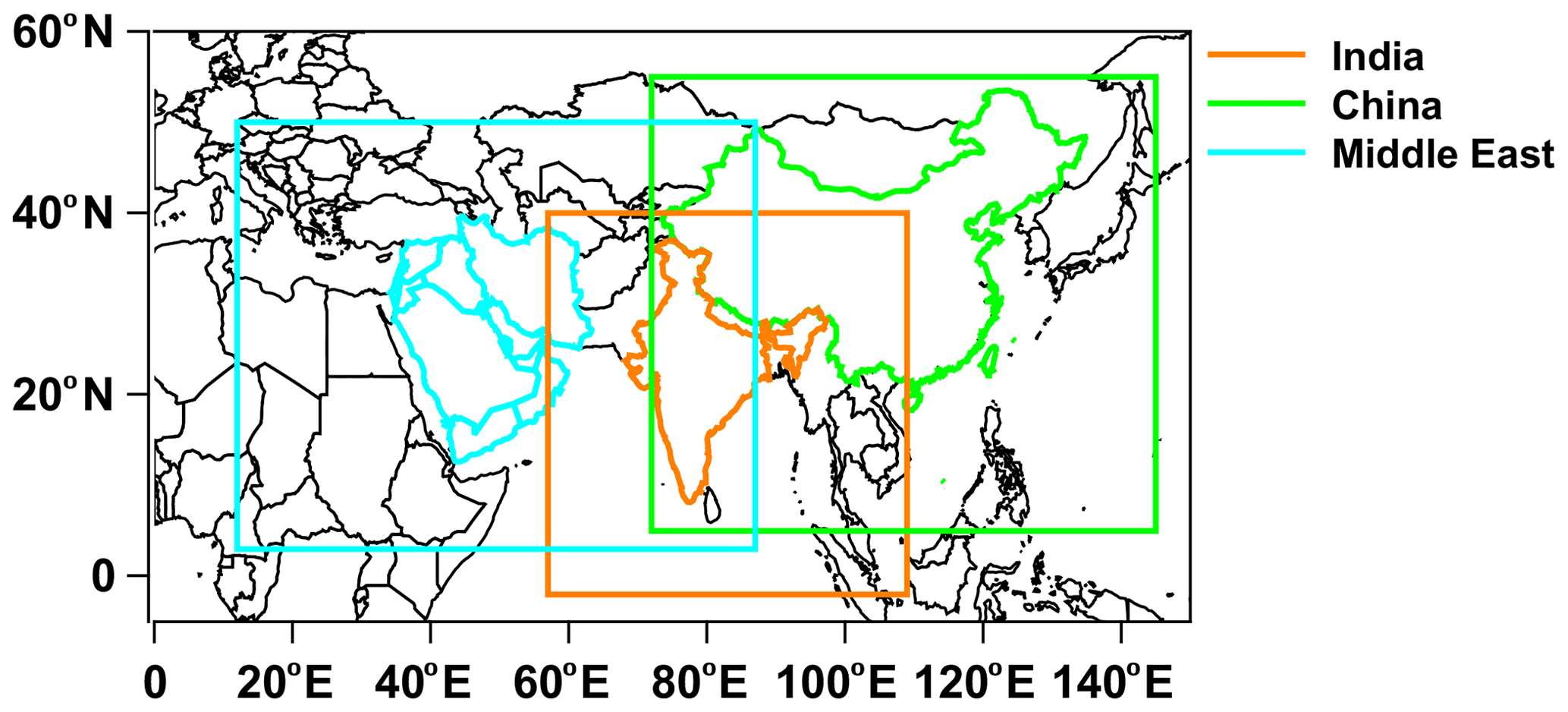
Figure 1The model domains for India, China, and the Middle East used in the present study. The land regions for the emissions are shown in color.
The wet removal scheme in WRF-Chem for MOZART chemistry, based on Neu and Prather (2012), was used to compute the dissolution of soluble trace gases into precipitation and their release into the gas phase upon evaporation of hydrometeors. Neu and Prather (2012) estimate trace gas removal by multiplying the effective Henry's law equilibrium aqueous concentration by the net precipitation formation (conversion of cloud water to precipitation minus the evaporation of precipitation). Dry deposition of trace gases was described with the Wesely (1989) parameterization. Diagnostic information on the wet and dry deposition of TFA was determined at every time step, and accumulated values were included in the output files.
2.2 Emissions
HFO-1234yf is just now entering the market driven by regional (e.g., the European Union's MAC Directive 2006/40/EC), national (e.g., Japan and USA) F-gas regulations, and the Kigali Amendment to the Montreal Protocol. HFC-134a is currently the primary working fluid of MAC and other applications (refrigerants, insulating foams, and aerosol propellants). Therefore, we have to estimate the future emission levels from the three regions of interest. Unlike the developed countries, India, China, and the Middle East are growing rapidly, and the use of air conditioning and refrigeration (and other uses of HFCs and HFOs) is expected to increase rapidly. Therefore, one has to consider the likely economic growth and other factors in estimating emissions levels. Here, we explore a few different potential scenarios for emissions of HFO-1234yf.
TFA production from HFO-1234yf increases linearly with the rise in HFO-1234yf emissions, i.e., there is no feedback on this process since the primary drivers for the degradation of this chemical, the OH radical, will not be altered by their relatively small emissions. In addition, the changes in the abundance of OH in the troposphere in the next few decades are unlikely to be different (e.g., <13 %) than the current levels based on the changes seen over the past few decades (Rigby et al., 2017). Therefore, we can estimate the extent of TFA formation from a set of modeling calculations that employed a fixed total amount of HFO-1234yf from each region. After that, we can calculate the extent of TFA formation for various possible emission scenarios.
We used the following four future HFO-1234yf emissions scenarios for the 2020 to 2040 period: (1) the estimate of the upper range scenario HFO-1234yf emissions based on Velders et al. (2015) estimate, (2) the lower range scenario of HFO-1234yf based on Velders et al. (2015) estimate, (3) the Greenhouse Gas Air Pollution Interactions and Synergies (GAINS) model (Amann et al., 2011) with maximum technically feasible reduction (MTFR) estimates of HFO-1234yf, and (4) the GAINS maximum HFO (max HFO) scenario. Given the relatively short lifetime of HFO-1234yf, the TFA production per year is dependent only on the emissions in that year. Figure 2 shows the HFO-1234yf emission projection from India, China, and the Middle East for the four scenarios between 2020 and 2040. The scenario based on S. Kumar et al. (2018) is similar to the fourth scenario we considered. Therefore, we have not specifically included this possibility.
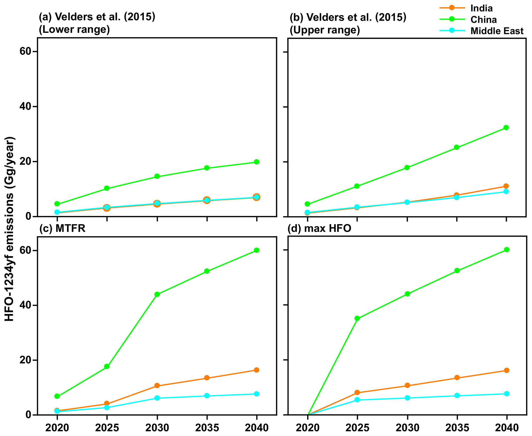
Figure 2The projected HFO-1234yf emissions scenarios between 2020 and 2040 from Velders et al. (2015). (a) Lower and (b) upper ranges. International Institute for Applied Systems Analysis (IIASA) GAINS model for (c) maximum technically feasible reduction (MTFR) and (d) max HFO in India, China, and the Middle East.
The emission estimates of HFO-1234yf in the GAINS model depend on when countries will comply with the Kigali Amendment, current and future emissions based on country-level activity data, uncontrolled emission factors, the removal efficiency of emission control measures, and the extent to which such measures are applied (Purohit and Höglund-Isaksson, 2017). The GAINS model uses the fuel input for the transport sector that is provided by the exogenous projections (e.g., IEA, 2017). First, using the annual mileage per vehicle (veh-km) and specific fuel consumption (SFC), GAINS estimates the number of vehicles (by type and fuel). Second, using the penetration rate of a MAC, the number of vehicles with MAC is calculated. Next, using the specific refrigerant charge (different for MAC used in vehicle types), the HFO-1234yf consumption in mobile air conditioners is calculated. Note that the HFO-1234yf is assumed to be substituted for HFC-134a, one to one, in all vehicles. For HFO-1234yf use in MAC, HFO-1234yf emissions are estimated separately for banked emissions, i.e., leakage from equipment in use, and for scrapping emissions, i.e., emissions released at the end of life of the equipment. The leakage rate in the GAINS model assumes a percentage of the charge per year. For example, if the refrigerant charge in MAC is 0.5 kg, then the emissions from the bank will be 0.05 kg (= 0.5 kg × 0.1) per year, where the leakage rate is 10 % per year. This leakage rate is a steady refrigerant loss through seals, hoses, connections, valves, etc., from every MAC over the entire use phase (annually). At the end of life, the scrapped equipment is assumed to be fully loaded with refrigerant, which needs recovery, recycling, or destruction. At the same time, if there are regulations in place (e.g., MAC Directive 2006/40/EC in the European Union), such as a package of measures including leak prevention during use and refill, maintenance, and end-of-life recovery, and recollection of refrigerants, then GAINS consider these good practices as a control option with a removal efficiency of 50 % for in use and 80 % for end of life, based on secondary sources (Purohit et al., 2020). However, no such measures are assumed for India, China, and the Middle East. Thus, these emissions can be considered the maximum likely emissions. The MTFR version of the GAINS scenario assumes that the maximum technically feasible reductions are applied across the sectors in India, China, and the Middle East. The Velders et al. (2015) emissions also follow the Kigali amendment. The Shared Socioeconomic Pathways (SSPs), SSP3 and SSP5, are the lower and upper range scenarios, respectively, used in Velders et al. (2015) calculated for 11 geographic regions and 13 use categories. S. Kumar et al. (2018) highlight that many applications in India will likely transition to something other than HFOs. These trends are not unique to India and will likely be replicated in China and the Middle East. Therefore, the four HFO-1234yf emission scenarios for the 2020 to 2040 period represent emissions that are higher than should be expected and, therefore, are upper limit estimates of the potential impact of TFA in these regions.
To minimize numerical errors (in using small emissions) and compare them with previous studies, we used HFO-1234yf emissions of ∼ 40 Gg yr−1 from each of these regions. This value corresponds to 2025 projected emissions from the GAINS model over India and the Middle East if all the applications were to use HFO-1234yf in place of HFC-134a for China; the emission values are for 2016 from Wang et al. (2018). Figure S1 in the Supplement shows the annual spatial distribution of HFO-1234yf over India, China, and the Middle East as simulated in (i) GEOS-Chem and (ii) WRF-Chem models. We distributed this total emission across the country/region of interest by scaling the emission to known anthropogenic CO emissions used in the model. The anthropogenic CO is a good tracer for HFO-1234yf emissions since they originate from similar applications (especially the transport sector) and in proportion to the distribution of economic activities in the region/country of interest. We show the total emissions in each of the three regions in both the models in the figure. The distribution varies to a small extent with the season (shown in Fig. S2), and the monthly variation in emission is similar in both models. We also simulated GEOS-Chem over the USA and Europe using the total HFO-1234yf emissions from Wang et al. (2018) and Henne et al. (2012), respectively.
2.3 Chemical scheme
The chemical degradation of HFO-1234yf and the production of TFA were added to both the GEOS-Chem NOx–Ox–hydrocarbon–aerosol chemistry scheme and the WRF-Chem MOZCART chemistry scheme. The detailed chemical scheme for the formation of TFA from HFO-1234yf is shown in Burkholder et al. (2015) and, therefore, not repeated here. The simplified representation of TFA production follows that of Kazil et al. (2014):
The conversion of HFO-1234yf to TFA includes an OH-initiated reaction of CF3CF=CH2 (reaction R1), with a temperature-dependent rate coefficient of cm3 molec.−1 s−1 to produce gas-phase CF3C(O)F (note that the initial OH reaction is the rate-limiting step in the conversion). The gas-phase removal of CF3C(O)F is not rapid but hydrolyzes to TFA in water (George et al., 1994; reaction R2). The hydrolysis process is added to the heterogeneous chemistry with a hydrolysis rate of 150 s−1 and Henry's law solubility constant of 3 M atm−1. TFA is highly soluble in cloud water. Upon cloud evaporation, the dissolved TFA is released into the gas phase (reaction R4). The gas-phase TFA is expected to be deposited either via dry (reaction R6) or wet deposition, using the Henry's law solubility constant of 9×10³ M atm−1 at a standard temperature of 298.15 K, K, dissociation coefficient of 0.65 mol L−1 at 298.15 K, and K. Thus, at cloud temperatures (generally <290 K), the effective Henry's law of TFA is high, characterizing TFA as a highly soluble gas. The dry deposition rate for TFA is assumed to be the same as that for nitric acid (Henne et al., 2012; Kazil et al., 2014; Luecken et al., 2010). We also included the potential loss of gas-phase TFA by its reaction with OH radicals (reaction R5) with a rate coefficient of cm3 molec.−1 s−1. Other potential losses of HFO-1234yf via reaction with Cl, O3, and NO3 are very small and all yield the same set of products. Therefore, we have not included them in the model. We also examined the possible removal of gas-phase TFA by its reaction with Criegee intermediate (CI). We used the Bristol group's calculated concentrations of the Criegee intermediates (Chhantyal-Pun et al., 2017; Khan et al., 2018).
3.1 Sulfate concentration in rainwater
Wet deposition is one of the primary removal processes for TFA. This deposition depends on precipitation amounts and how well our model captures the wet deposition process, making it crucial to evaluate the models used here to capture these two factors.
First, we compared the annual total precipitation amounts calculated by GEOS-Chem and WRF-Chem with the observed daily total accumulated precipitation from the Tropical Rainfall Monitoring Mission (TRMM_3B42_daily product) in the three regions (Fig. S3a). The TRMM product is at a 0.25∘ × 0.25∘ resolution. The spatial distribution of seasonal total precipitation in the three domains from the two models and TRMM is shown in Fig. S4. Both the models captured the seasonal precipitation patterns. As seen in Fig. S3a, the total precipitation amounts were a factor of 1.5–2 higher in GEOS-Chem compared to WRF and TRMM. (The ratio of total precipitation between GEOS-Chem and WRF-Chem (TRMM) was 2.6 (1.5), 2.2 (1.5), and 2.2 (1.4) for India, China, and the Middle East, respectively). WRF-Chem underestimated the precipitation amounts compared to TRMM in the three regions. R. Kumar et al. (2012, 2018) have addressed the precipitation biases in WRF-Chem compared to TRMM over South Asia. We attribute the higher precipitation in GEOS-Chem to (a) the different model physics used, (b) the effects of a meteorology-driven chemistry transport model (GEOS-Chem) versus an online chemistry transport model (WRF-Chem), where chemistry is solved at the same time step as the meteorology, (c) and to the different grid spacings used by the two models, noting that the coarse GEOS-Chem grid cells contain several convective storms compared to those in WRF-Chem. The monthly variation in total precipitation is shown in Fig. S3b, and both models have similar trends as those observed by TRMM.
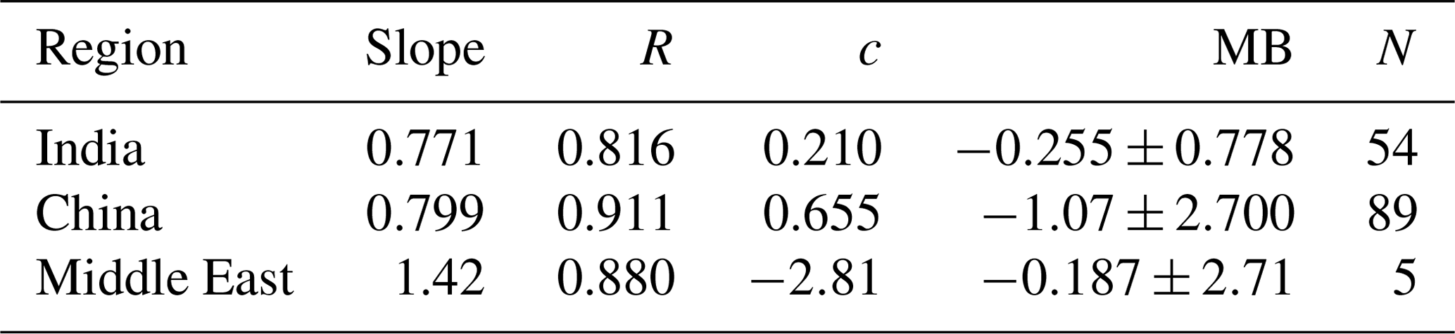
To evaluate the accuracy of the TFA wet deposition, it is useful to compare sulfate wet deposition amounts produced by the oxidation of SO2. The emissions of SO2 are comparable in both the models (shown in Fig. S5). We have measurements of sulfate rainwater concentrations in some of the regions. Furthermore, the lifetime of SO2 in the troposphere is comparable to that of HFO-1234yf. We hasten to add that, while the HFO-1234yf degradation is controlled by gas-phase OH reactions, SO2 degradation includes both gas- and condensed-phase processes. However, the removal of both sulfate and TFA are due to condensed-phase reactions. The WRF-Chem model has been shown to capture the sulfate rainwater concentration over the continental USA by Kazil et al. (2014); we expect it to do well over this study's regions. However, GEOS-Chem has not been evaluated previously. There are no networks for measuring sulfate rainwater concentration in India and the Middle East. Yet, there are some observations of rainwater sulfate in the published articles in all three domains. The available data are sparse, and the observations for 2015 (the modeled year) are even fewer to make a comparison with WRF-Chem simulations. However, GEOS-Chem simulations were available from our previous work for 2000–2015. We used those results to compare with observations during that period. The observation locations (over land only) in the three domains are shown in Fig. S6. Figure 3 shows the scatterplot of simulated and observed sulfate rainwater concentration in the three domains. Table 1 lists the statistics of the comparison between GEOS-Chem and the observations. Rainwater sulfate amounts calculated by GEOS-Chem correlate well (R>0.80) with observations. We see a bias of −13 %, −13 %, and −3 % in India, China, and the Middle East domains, respectively. The negative bias in GEOS-Chem sulfate rainwater concentration could be because the model integrates over a large area, while the observations are point locations. It could also be, as noted earlier, because GEOS-Chem yields higher amounts of precipitation and, thus, could lead to smaller rainwater concentrations. We suggest that these values are good to at least a factor of 2. In summary, the GEOS-Chem model shows considerable skill in reproducing mean sulfate rainwater concentrations and spatial variability in sulfate rainwater concentrations; therefore, it can be utilized to calculate TFA wet deposition.
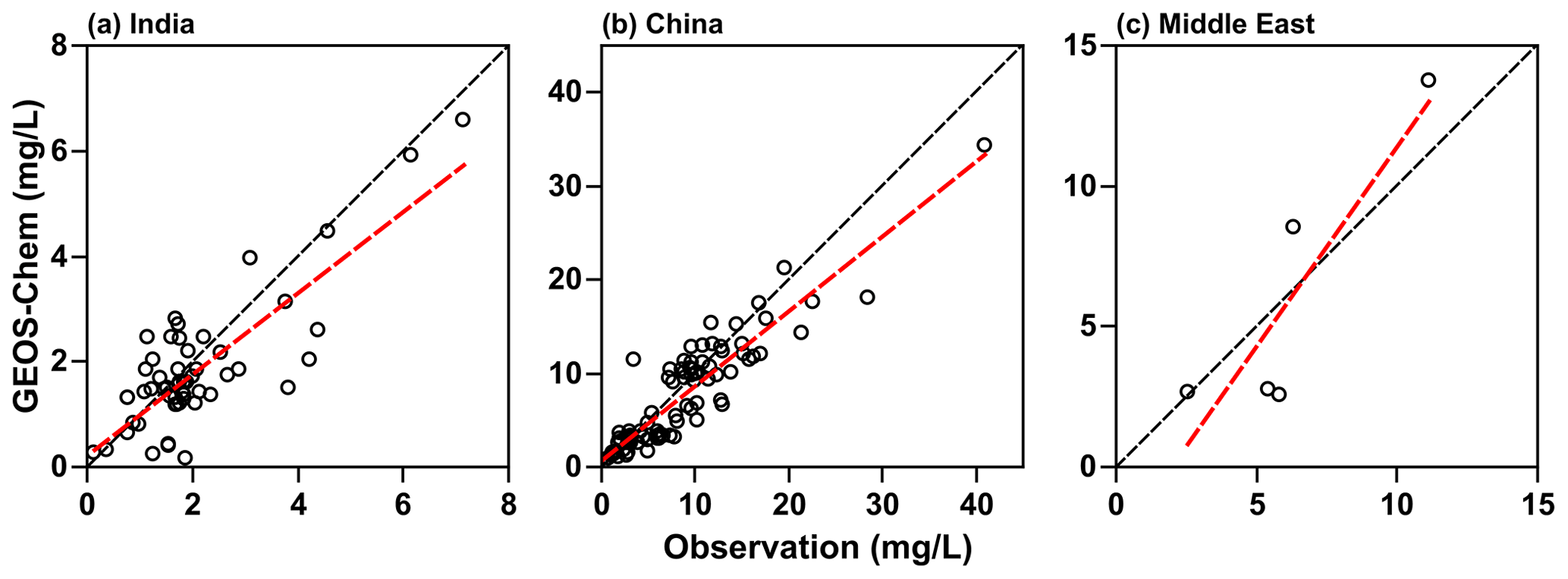
Figure 3Scatterplot of simulated and observed sulfate rainwater concentration in (a) India, (b) China, and (c) the Middle East for 2000–2015. The linear regression line is shown in red. The black dashed line corresponds to slope = 1. The data for the Middle East are very limited.
Table 1The slope, correlation coefficient (R), intercept (c), mean bias (MB), and the number of points (N) of simulated (GEOS-Chem) and observed sulfate rainwater concentration over the three domains.
3.2 Comparison of calculated TFA with previous studies
Before presenting the results of the calculations for India, China, and the Middle East from the present study, we note that our models agree with the previous studies over the USA (Kazil et al., 2014; Luecken et al., 2010), China (Wang et al., 2018), and Europe (Henne et al., 2012). Figure 4 shows the comparison of annual mean (a) TFA deposition (dry and wet combined) and (b) TFA rainwater concentration over the USA, China, and Europe. We have normalized the emissions to match those of the previous studies for meaningful comparisons. (The emissions used to compare TFA from the USA, China, and Europe are 24.5, 42.7, and 19.2 Gg yr−1, respectively.) We note that average deposition rates differ in the model because of the differences in the calculations' domain sizes. Given that the models vary in their versions, meteorology, physics, and the expected model variabilities, the observed agreement is reasonable. The TFA rainwater concentration in China is a factor of 2 higher in WRF-Chem because the total precipitation amounts were factors of 1.5–2 higher in GEOS-Chem compared to WRF and TRMM, as mentioned in Sect. 3.1. We also show the comparison with our calculations over the USA for the summer months with previous studies (Kazil et al., 2014; Luecken et al., 2010; Wang et al., 2018) (Fig. S7).
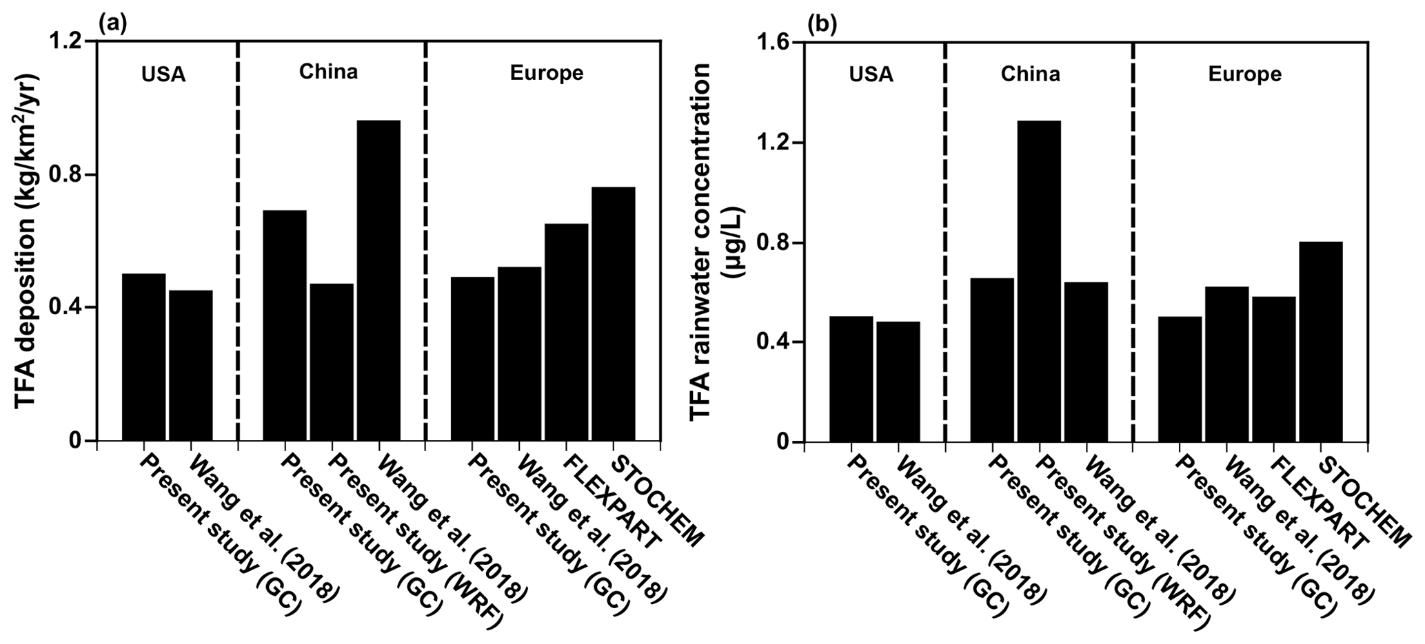
Figure 4Comparison of the present study with other studies over the USA, China, and Europe for (a) TFA deposition and (b) TFA rainwater concentration. Note the emissions are 24.53, 42.65, and 19.16 Gg yr−1 for the USA, China, and Europe, respectively.
3.3 Atmospheric mixing ratios
Figure 5 shows the annual mean mixing ratios of HFO-1234yf over India, China, and the Middle East as simulated by GEOS-Chem and WRF-Chem. We present here only results with emissions in GEOS-Chem (WRF-Chem) of 41.3 (41.9), 40.6 (39.9), and 37.8 (38.1) Gg yr−1 from India, China, and the Middle East, respectively. Expected TFA for other emissions can be simply scaled to the emissions of interest. The annual mean mixing ratio of HFO-1234yf in India, China, and the Middle East as simulated by GEOS-Chem (WRF-Chem) were 2.87 (3.94), 2.49 (3.70), and 1.82 (2.49) ppt (parts per trillion), respectively, and below 1 ppt (as seen in GEOS-Chem) outside of the three regions. The annual mean mixing ratio in the China domain was comparable to Wang et al. (2018). The highest (>40 ppt) simulated annual mean HFO-1234yf mixing ratio for India was in the Indo-Gangetic Plain (IGP), for China in the northeastern region, and for the Middle East in northern Iran. The emission hot spots (Fig. S1) in the three regions led to the largest annual mean HFO-1234yf mixing ratios in those regions. The WRF-Chem simulated higher annual mean HFO-1234yf mixing ratios compared to GEOS-Chem. Differences in annual mean HFO-1234yf mixing ratios between models for the same amount of emissions have been reported also by Henne et al. (2012). However, the overall spatial patterns are comparable between GEOS-Chem and WRF-Chem. It should be noted that the change in HFO-1234yf emissions in any of the three regions would change the HFO-1234yf mixing ratio within that region and will have minimal effect on other regions.
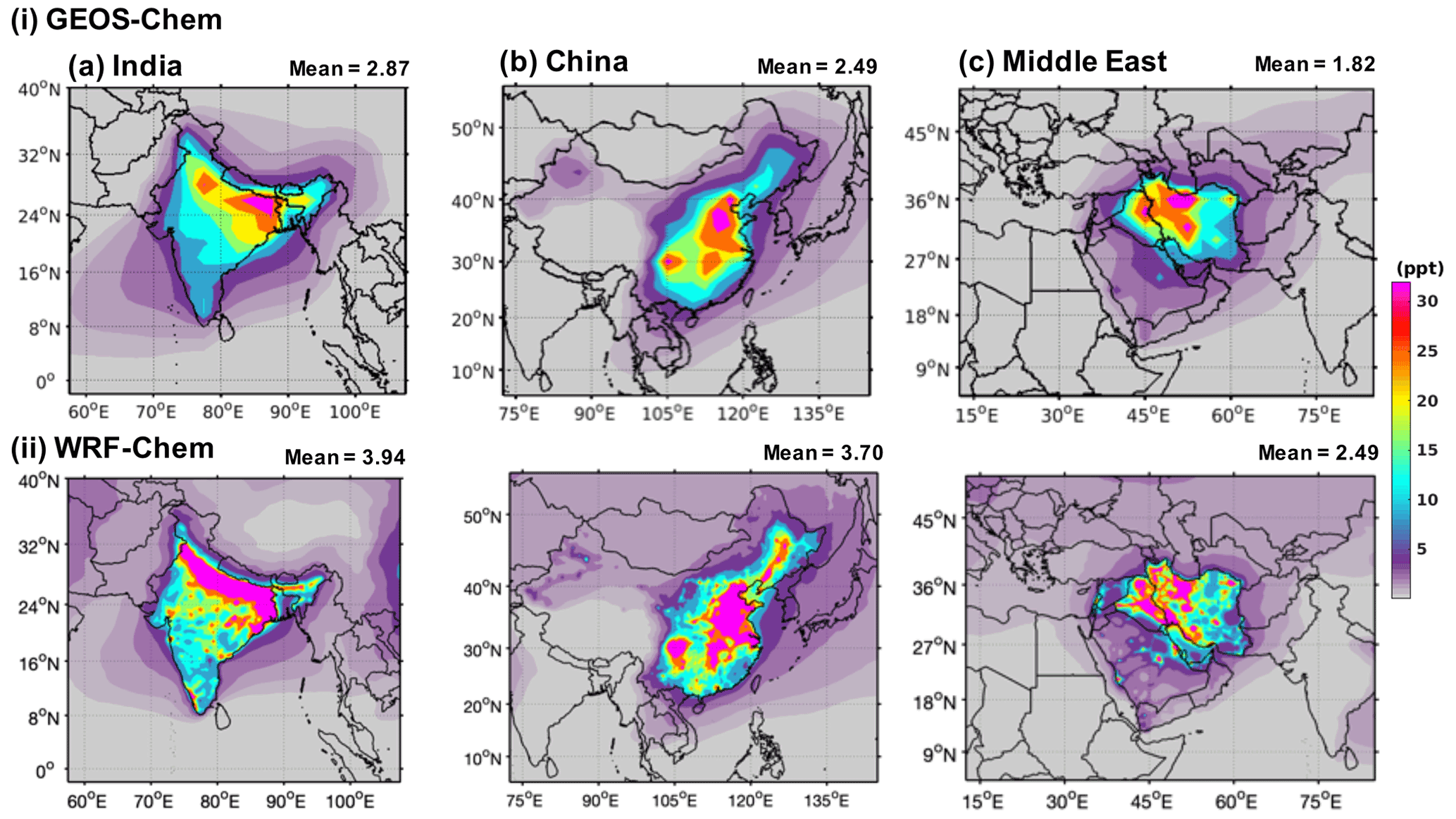
Figure 5Annual mean surface mixing ratios of HFO-1234yf simulated in (i) GEOS-Chem and (ii) WRF-Chem over (a) India, (b) China, and (c) the Middle East. The number at the top of each panel gives the mean HFO-1234yf mixing ratios within the domains.
3.4 TFA deposition
GEOS-Chem simulated mean total deposition rates (dry and wet deposition combined) to be 0.874, 0.501, and 0.477 kg km−2 yr−1, respectively, in India, China, and the Middle East domains for emissions of 41.3, 40.6, and 37.8 Gg yr−1, respectively. WRF-Chem simulated mean deposition rates (dry and wet) were 0.802, 0.342, and 0.284 kg km−2 yr−1 in India, China, and the Middle East domains, respectively (Fig. S8). Figure 6 shows the annual total dry and wet TFA deposition rates in the three domains. The total annual dry deposition in GEOS-Chem and WRF-Chem over the India domain was largest in eastern India and Bangladesh, reaching up to 2 kg km−2 yr−1. The wet deposition in the India domain mostly occurred in the Himalayan foothills, eastern IGP, parts of central India, and southwestern India and was >3.5 kg km2 yr−1. In the China domain, the total dry and wet deposition rates in GEOS-Chem and WRF-Chem were highest in southeastern China. The total dry deposition rate in the Middle East domain was highest in northern Iran. The wet deposition rate was the largest in parts of Iran, with differences between the models. The wet deposition dominated the total TFA deposition. The combined annual total deposition pattern was similar to that of wet deposition in the three domains (Figs. 6 and S8). The seasonal total deposition rates of TFA from dry and wet depositions in the three domains are shown in Fig. S9. The seasonal deposition rates were highest for June–September, June–August, and April–October in India, China, and the Middle East domains, respectively.

Figure 6GEOS-Chem and WRF-Chem simulated annual total deposition rates of TFA (kilograms per square kilometer per year; hereafter kg km−2 yr−1) from (a) dry and (b) wet deposition in India, China, and the Middle East domains. The number at the top of each panel gives the mean dry and wet deposition rates within the domains.
Figure 7 shows the percentage contribution of dry and wet deposition to total TFA deposition between GEOS-Chem and WRF-Chem in the three domains. It should be noted that the sum of the two (dry and wet) percent contributions do not add up to exactly 100 % because of transport in and/or out of the domains. For the total amount of HFO-1234yf emissions mentioned in Fig. S1 and discussed in Sect. 2.2, the total TFA deposition (dry and wet combined) in India, China, and the Middle East domains from GEOS-Chem were 23.4, 20.5, and 18.7 Gg yr−1, respectively. The total annual dry (wet) deposition amounts account for 21 (36) %, 20 (31) %, and 20 (29) % of the annual emissions of HFO-1234yf in GEOS-Chem. In WRF-Chem, the annual total TFA deposition was 19.4, 12.1, and 9.9 Gg yr−1, respectively, in India, China, and the Middle East domains. The dry (wet) TFA deposition was 10 (37) %, 3 (23) %, and 4 (26) % of the emissions in India, China, and the Middle East domains, respectively. Table S2 shows the seasonal TFA deposition (dry and wet) calculated from GEOS-Chem and WRF-Chem models in the three domains. The lower TFA deposition in WRF-Chem compared to GEOS-Chem is due to the venting of surface emissions into the free troposphere (Grell et al., 2004; Kazil et al., 2014) that leads to lower dry deposition in WRF-Chem (Fig. 7a). The differences in deposition between models can also be attributed to differences in model resolutions, model transport, meteorological conditions (e.g., precipitation), and cloud treatment. These differences highlight the need for multi-model simulations to estimate the likely variation in these parameters.
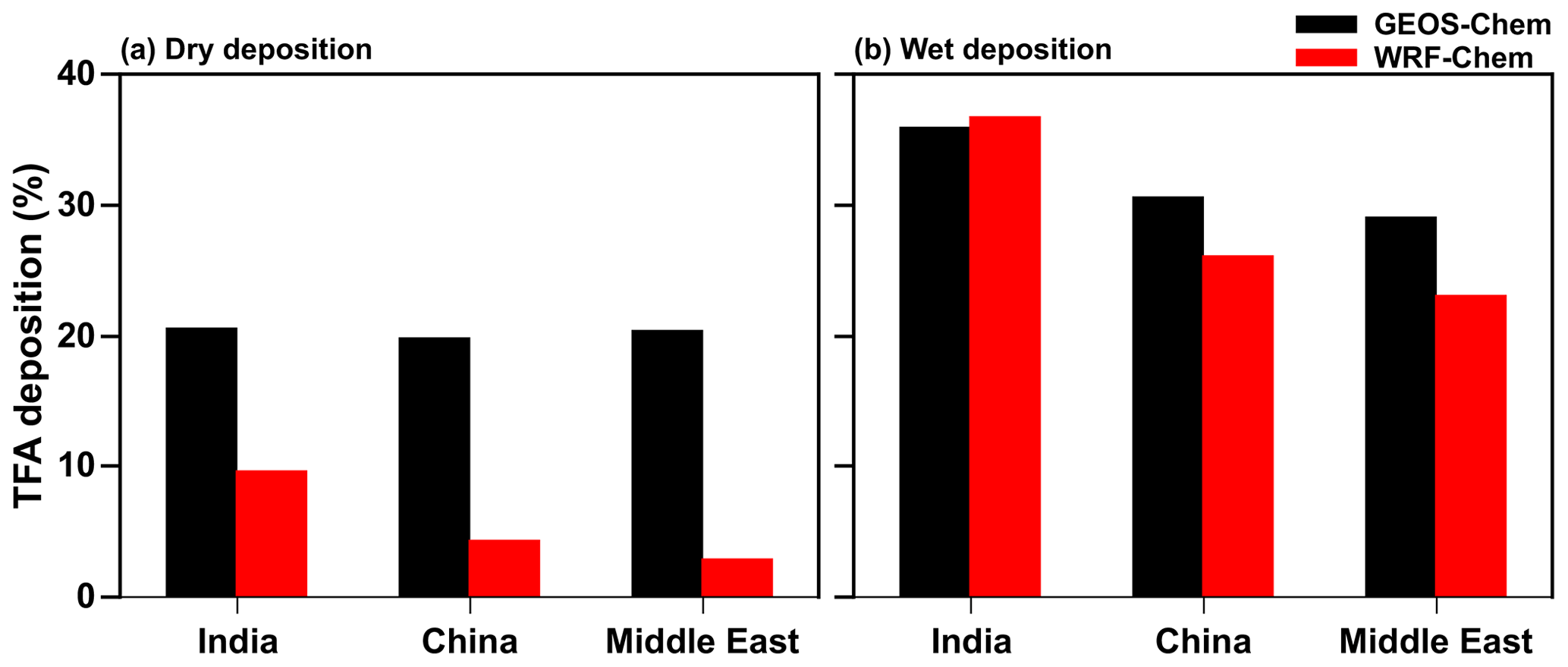
Figure 7Percentage contribution of (a) dry and (b) wet deposition to total annual TFA deposition simulated in GEOS-Chem and WRF-Chem in the three domains.
Figure 8 shows the total TFA deposition (dry and wet combined) for the four emission scenarios (Fig. 2) calculated from GEOS-Chem and WRF-Chem. Our results show that the differences in the calculated extent of TFA formed and deposited are about a factor of 2 between the models. In all cases, the computed TFA dry and wet deposition varies linearly with the emissions. Therefore, we can calculate the amounts of TFA formed and deposited for any envisioned emission of HFO-1234yf.
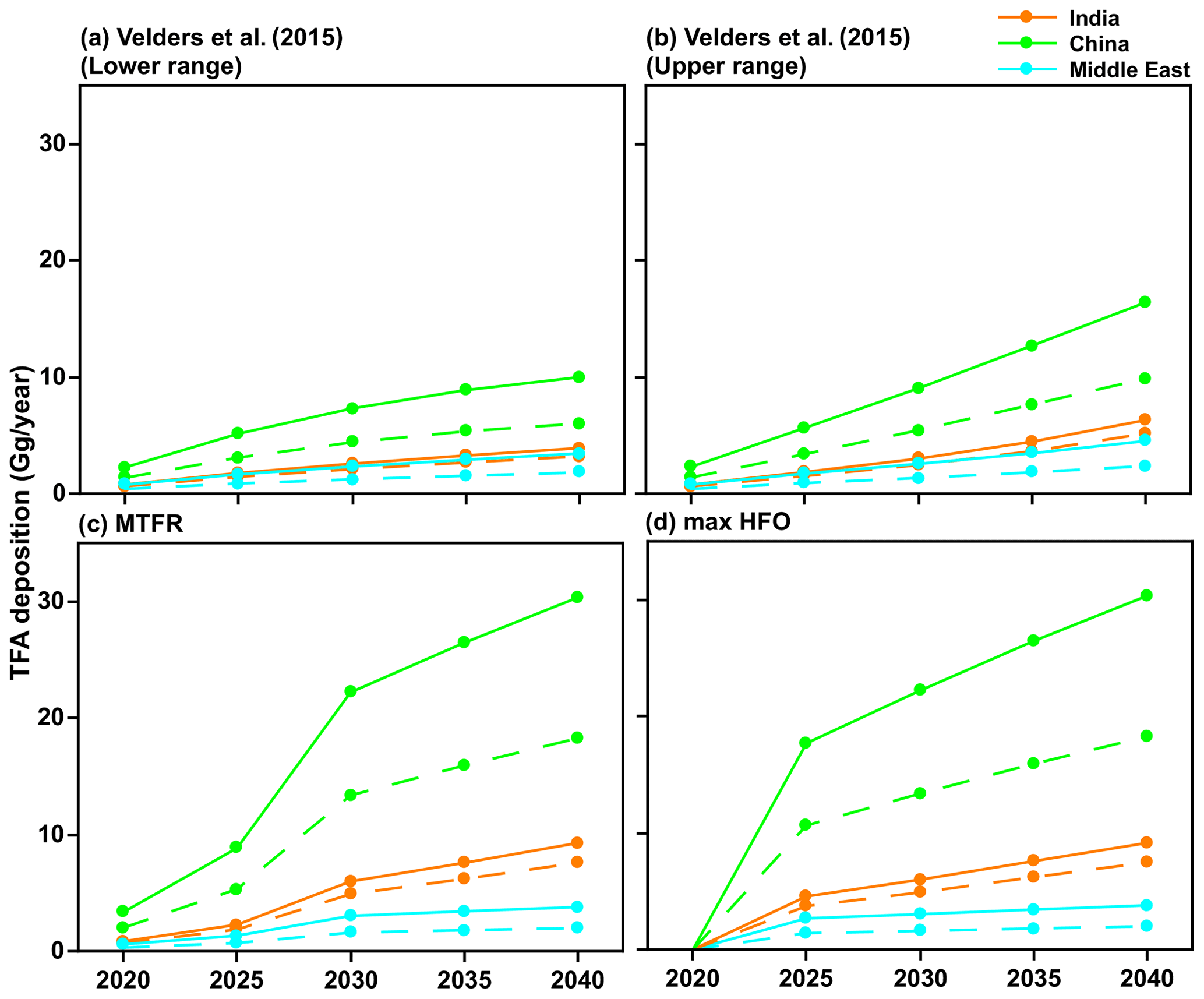
Figure 8Total TFA deposited (dry and wet combined) in four emission scenarios for 2020 to 2040 within India, China, and the Middle East domains calculated using GEOS-Chem (solid lines) and WRF-Chem (dashed lines). The values from the two models are reasonably close for India and the Middle East, while they differ by almost a factor of 2 for China.
3.5 Rainwater concentrations
Figure 9 shows the monthly variation in mean TFA rainwater concentration in the three domains calculated from GEOS-Chem and WRF-Chem. The TFA rainwater concentration also varies linearly with the emissions. Figure 9 shows the following: (a) higher concentrations are to be expected when there is little rain/precipitation (Fig. S10) to remove TFA. This point has been noted in previous studies (Kazil et al., 2014; Russell et al., 2012; Wang et al., 2018). So, if all the TFA were concentrated into a small amount of rain, the concentrations have to be larger. Such events are infrequent. They are, relative to the rainier regions, more frequent in the Middle East. The large rainwater concentration does not mean that the amount of deposited TFA is larger. (b) The rainwater concentrations varied inversely with the precipitation amount, as seen by comparing the rainwater TFA levels with the total precipitation (Fig. S10). A clear signal for the rainfall variation was seen over India, where the monsoon season (June, July, August, and a part of September) brings large and almost constant precipitation. This large precipitation makes the TFA rainwater concentrations extremely small. In other words, this is simply a dilution effect. (c) When the rainfall is small, there are considerable variations, as one would expect. Lesser total precipitation arises because of fewer showers and often in spatially and temporally sporadic events. So, the concentrations can vary a great deal. This was also evident over China during dry seasons. (d) The calculated TFA rainwater concentrations were comparable to previous calculations for China (scaled to emissions; Fig. 4b). The variation in rainfall amounts and their geographical distribution as climate changes are uncertain, but there are some estimates. For example, Terink et al. (2013) suggest that there could be a ∼ 20 % decrease in precipitation over the Middle East region over the next 20 years. A 20 % decrease in precipitation will correspond to TFA rainwater concentration of less than 40 µg L−1 (95th percentile). The annual mean precipitation over China is likely to increase; for example, estimates are roughly increases of 0.078 mm d−1 in the 2020s and 0.218 mm d−1 in 2050s, with larger changes in the summer months (rainy season; Guo et al., 2017). The projected rainfall changes across the Indian monsoon region could increase by 6 % (RCP4.5) and 8 % (RCP8.5) in the mid-21st century (Krishnan et al., 2020).
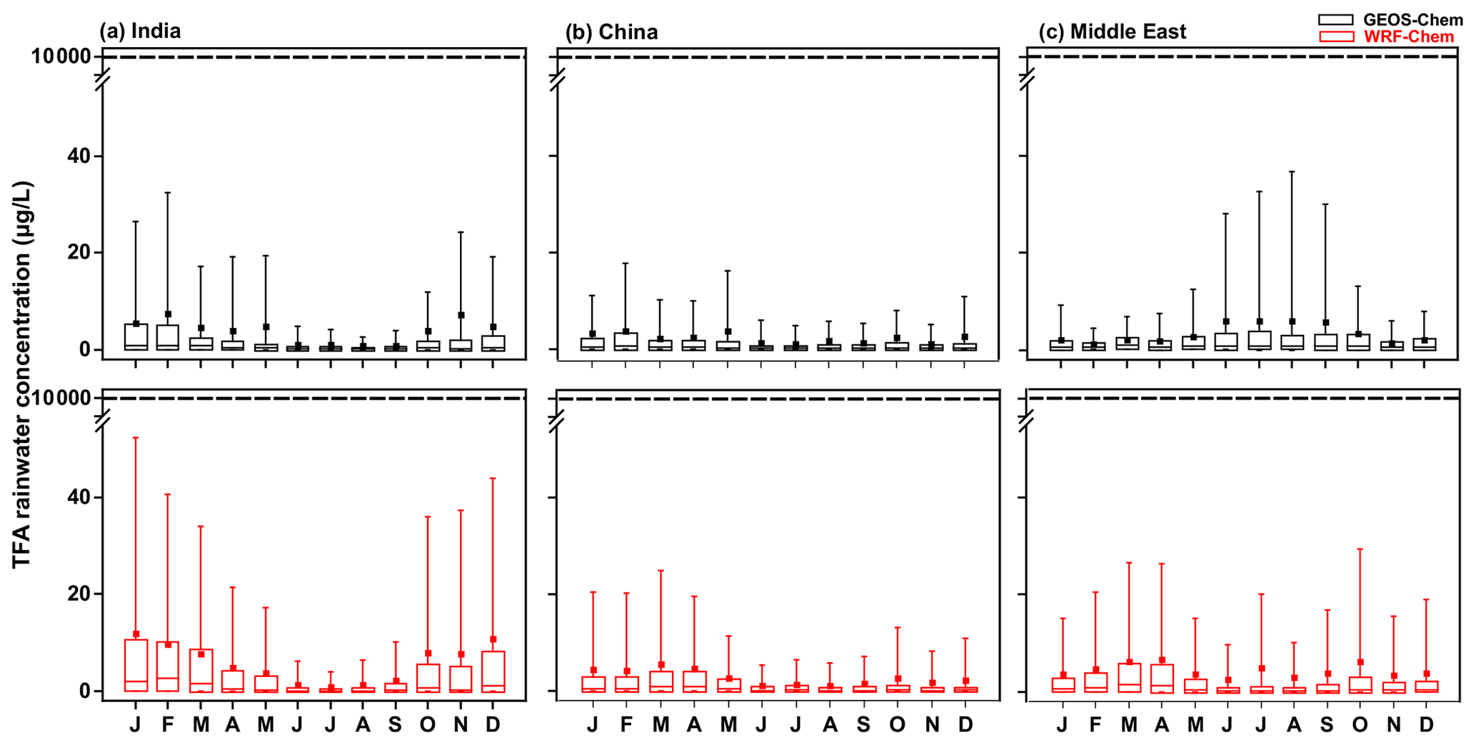
Figure 9Box and whisker plot of TFA rainwater concentration calculated from GEOS-Chem and WRF-Chem in the three domains. In the box plot, the inside line and square are the median and mean, respectively. Box boundaries are the 25th and 75th percentiles, and whiskers indicate the 5th and 95th percentiles. The dashed horizontal line is the no observable effect concentration (NOEC) level. It is important to note that these values, including the 95th percentile values, are at least 100 times lower than the NOEC for harming aquatic bodies, even when normalized for higher projected emissions in 2040.
It is important to know the regions of high TFA rainwater concentrations. Therefore, we plotted the spatial pattern of annual mean TFA rainwater concentration in the three domains from both models (Fig. S11). It is noticeable that most of the regions in all three domains did not have high TFA rainwater concentrations. There were some grids with TFA rainwater concentrations that exceeded 50 µg L−1 for emissions of ∼ 40 Gg yr−1. The high TFA rainwater concentration seen in the western part of the India and China domains is because of input at the lateral boundaries from a global model. As mentioned in Sect. 3.1, the precipitation in GEOS-Chem was higher, resulting in lower TFA rainwater concentration. Focusing on the highest possible rainwater concentrations is misleading since that does not tell us the amount of wet TFA deposition, which is shown in Fig. 6. However, it is clear that, if the emissions of HFO-1234yf reach the large numbers noted by the IIASA GAINS model (max HFO; Fig. 2d) for 2040, there will be significant areas with larger TFA rainwater concentrations. The wet deposition does not tell the whole story either, since a substantial fraction of the rainwater ends up in the oceans every year. The estimation of the TFA retained on land will be critical for further estimating the long-term impact. Such a hydrology study is warranted but beyond the scope of this work.
Comparison of expected TFA rainwater levels with no observable effects concentrations
The primary reason for carrying out these calculations was to estimate the potential impact of HFO-1234yf usage in the three regions of the study for the current and future emissions. The effects of interest here are TFA formation from HFO-1234yf and its consequences to human and ecosystem health. Figure 10 shows the mean TFA rainwater concentration for the four emission scenarios calculated from GEOS-Chem and WRF-Chem. In all the scenarios, the annual mean TFA rainwater concentration was well below the no observed effect concentration (NOEC) for aquatic species, which is > 10 000 µg L−1 (Solomon et al., 2016), with an outlier for the most sensitive alga as 120 µg L−1 (Boutonnet et al., 2011). The negligible impact of TFA formation during the atmospheric oxidation of HFCs, HCFCs, and HFOs has been established for some time. The World Meteorological Organization (WMO) and United Nations Environment Programme (UNEP) quadrennial ozone layer assessment (2007) concluded that TFA from the degradation of HCFCs and HFCs would not result in environmental concentrations capable of significant ecosystem damage. Hurley et al. (2008) concluded in their study that the products of the atmospheric oxidation of CF3CF=CH2 will have a negligible environmental impact. Solomon et al. (2016) also concluded in their study that the concentrations of TFA and its salts in the environment that result from degradation of HCFCs, HFCs, and HFOs in the atmosphere do not present a risk to humans and the environment.
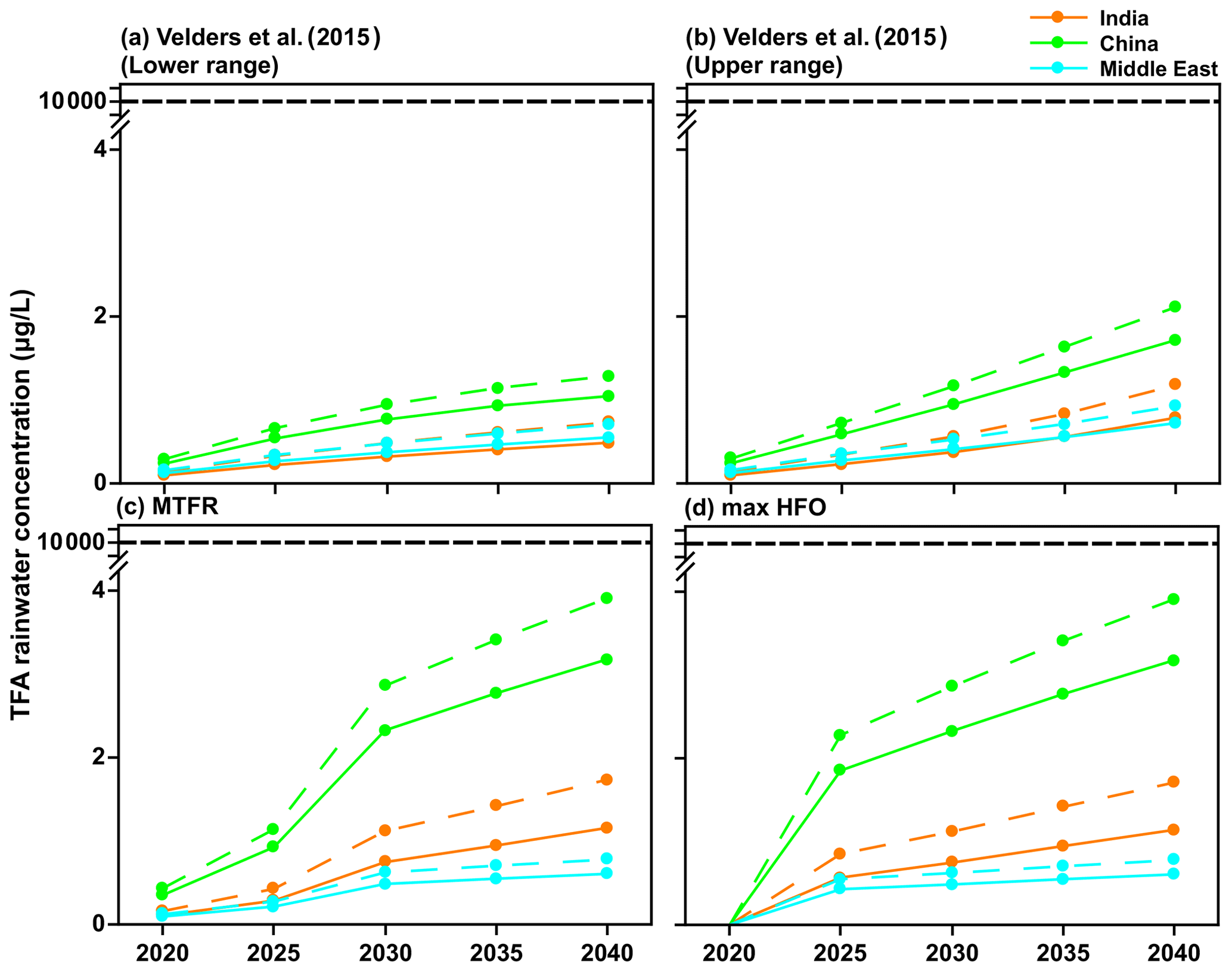
Figure 10Mean TFA rainwater concentration in four scenarios for 2020 to 2040 for India, China, and the Middle East domains calculated using GEOS-Chem (solid lines) and WRF-Chem (dashed lines). The NOEC is denoted above, and it is 2 orders of magnitude larger than calculated TFA concentrations for any of the scenarios.
Neale et al. (2021) have summarized the impact of TFA on human and ecosystem health. Their conclusion suggests that the NOEC on aquatic systems is > 10 000 µg L−1. As shown in Figs. 9, 10, and S11, the expected rainwater concentrations are at least 2 orders of magnitude lower than the NOEC. Also, the rainwater concentrations of TFA, even for the 2040 emissions, are roughly comparable to those currently observed in China (Chen et al., 2019) and about 10 times greater than those presently observed over Germany (Freeling et al., 2020). They also note that large TFA concentrations have been observed in people's blood in China, with no ill effects on the endpoints measured in that work (Duan et al., 2020).
TFA quantities deposited via dry deposition to land and vegetation would be much smaller than those noted in Neale et al. (2021) to have any significant detrimental health effect. Indeed, they note that there are other sources of TFA that are much higher than those expected from HFO-1234yf degradation. Neale et al. (2021) also point out that the TFA deposited to snow in the Arctic would not significantly contribute to marine water bodies even if it all melted down, since the volume of the melt would be much smaller than those of the receiving water bodies.
Lastly, since TFA can accumulate over land and water bodies, we can estimate the influence of accumulation on the potential future impacts. The total TFA amount in rainfall would not change. However, the amounts in water bodies could increase. For the 20 years modeled here, the total TFA in water bodies would be larger than those observed for 2020 if TFA merely accumulates. It is hard to calculate precisely where the water bodies would accumulate TFA without a hydrological model. However, these values would still be orders of magnitude smaller than the NOEC of > 10 000 µg L−1. For example, if all the TFA produced in these regions were to end up in the top 15 m of the world's oceans, we expect the TFA levels to increase by about 0.015 µg L−1 by 2040.
Based on these observations, and assuming that the NOEC concentration holds, it appears that the TFA from the expected emissions of HFO-1234yf in these three regions would not constitute a health threat to plants or humans (even if we assume that there is no water treatment to remove TFA in drinking water).
3.6 Interannual variability
The model results discussed in the previous sections are for 1 year, namely 2015. To assess the influence of interannual variability in meteorology, we simulated the TFA deposition and rainwater concentration for 2016 with the GEOS-Chem model for the total HFO-1234yf emissions described in Sect. 2.2. Figure 11 shows the fraction of TFA in the three domains for 2015 and 2016 that is (a) dry deposited and (b) wet deposited, as well as (c) the annual mean TFA rainwater concentrations. The total precipitation in both years was comparable (shown in Fig. S12). The results of our 2-year simulations lead us to conclude that the interannual differences are small. Therefore, we suggest that the results of 2015 are applicable going forward to 2040.
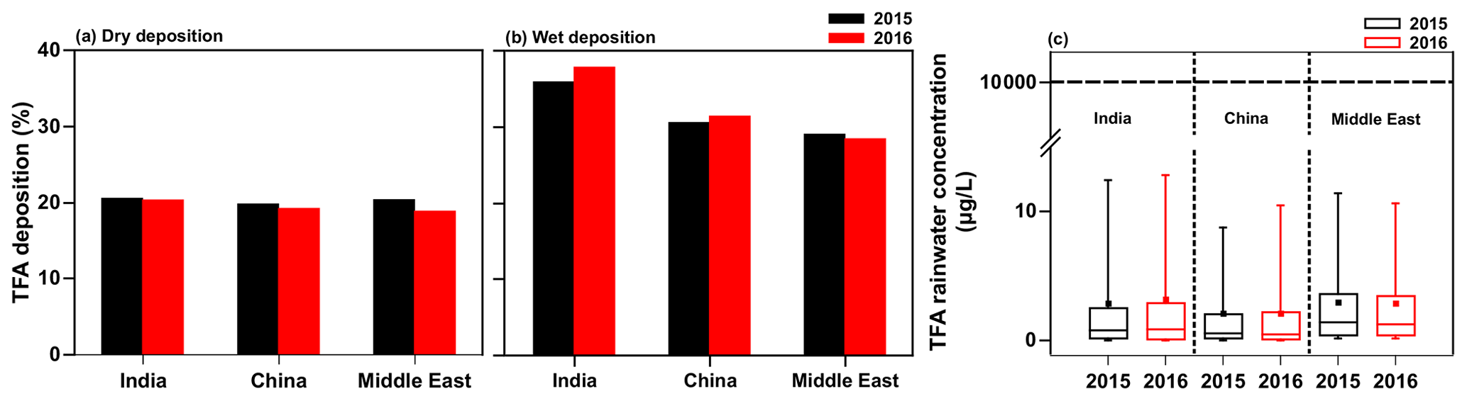
Figure 11Annual percentage of total TFA (a) dry and (b) wet deposition and (c) annual mean TFA rainwater concentrations in India, China, and the Middle East domains from GEOS-Chem for 2015 and 2016. The dashed horizontal line is the NOEC level.
3.7 Simultaneous emissions from multiple regions
It is important to note that most TFA is deposited outside of the domains, even though the estimated lifetime of HFO-1234yf is about 10 d. Therefore, TFA is dispersed significantly from the source region. Figure 12a shows that roughly 25 %–50 % of the HFO-1234yf emitted from a given region was converted and deposited (via dry and wet deposition) as TFA within the domain (see Fig. 1 for domain boundaries). Figure 12b shows the percentage of TFA deposition (dry and wet combined) calculated from GEOS-Chem and WRF-Chem within the three domains over land. The remaining TFA was transported outside the domain. It is difficult to quantify the exact locations of these depositions outside the domain since the concentrations become very small, even though in the aggregate that accounts for somewhere between 30 % and 45 %. The fraction that was deposited within the region of emission was even smaller and ranged between 7 % and 27 %. Therefore, it can be concluded that a significant fraction ended up in the oceans. This is especially true for India and the Middle East emissions. Interestingly, a substantial amount of the TFA from the Middle East emissions is deposited in the Arabian Sea. Therefore, we conclude that even though HFO-1234yf is short lived, it is still sufficiently long lived to travel thousands of kilometers. Such an expectation is in accord with the calculated distances traveled by an air mass for even about 2 m s−1.
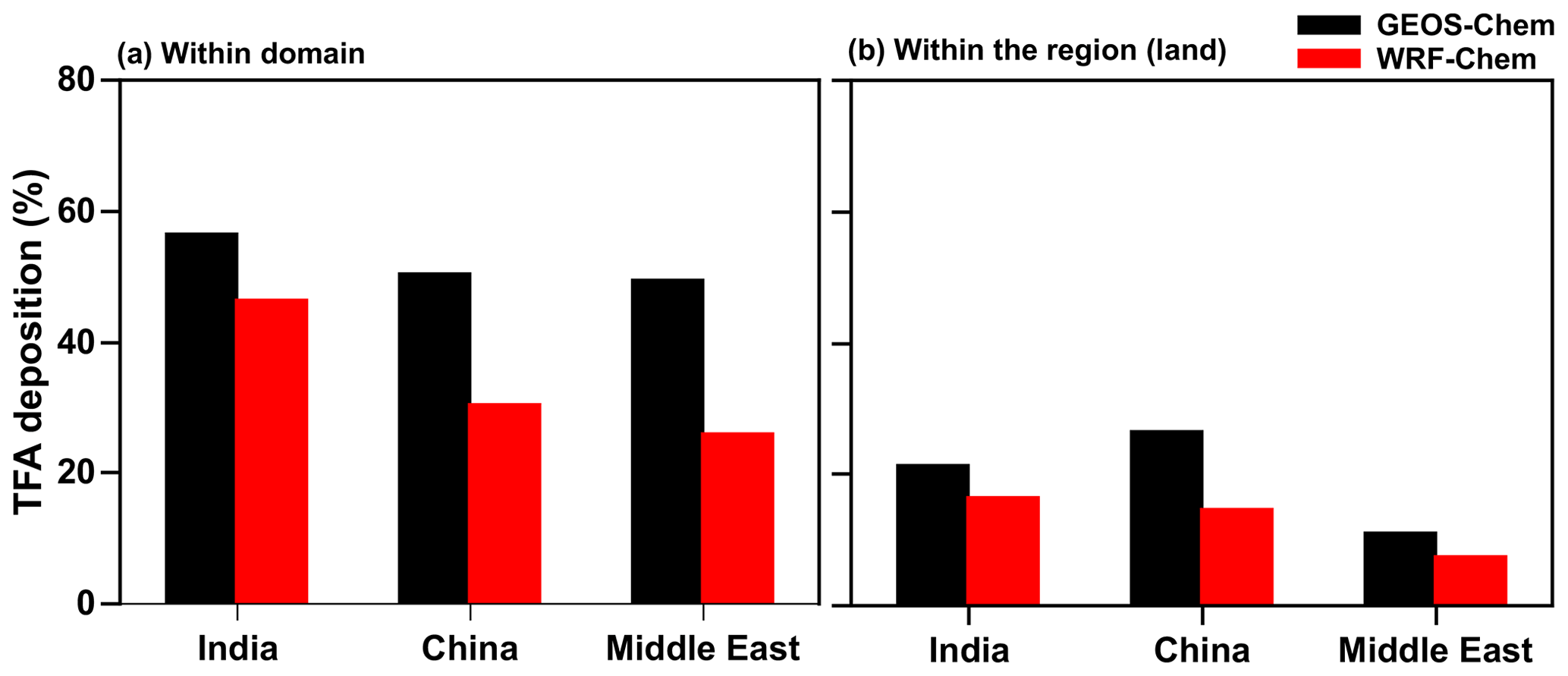
Figure 12Annual percentage of total TFA deposition (dry and wet combined) calculated from GEOS-Chem and WRF-Chem within the three (a) domains and (b) regions (land).
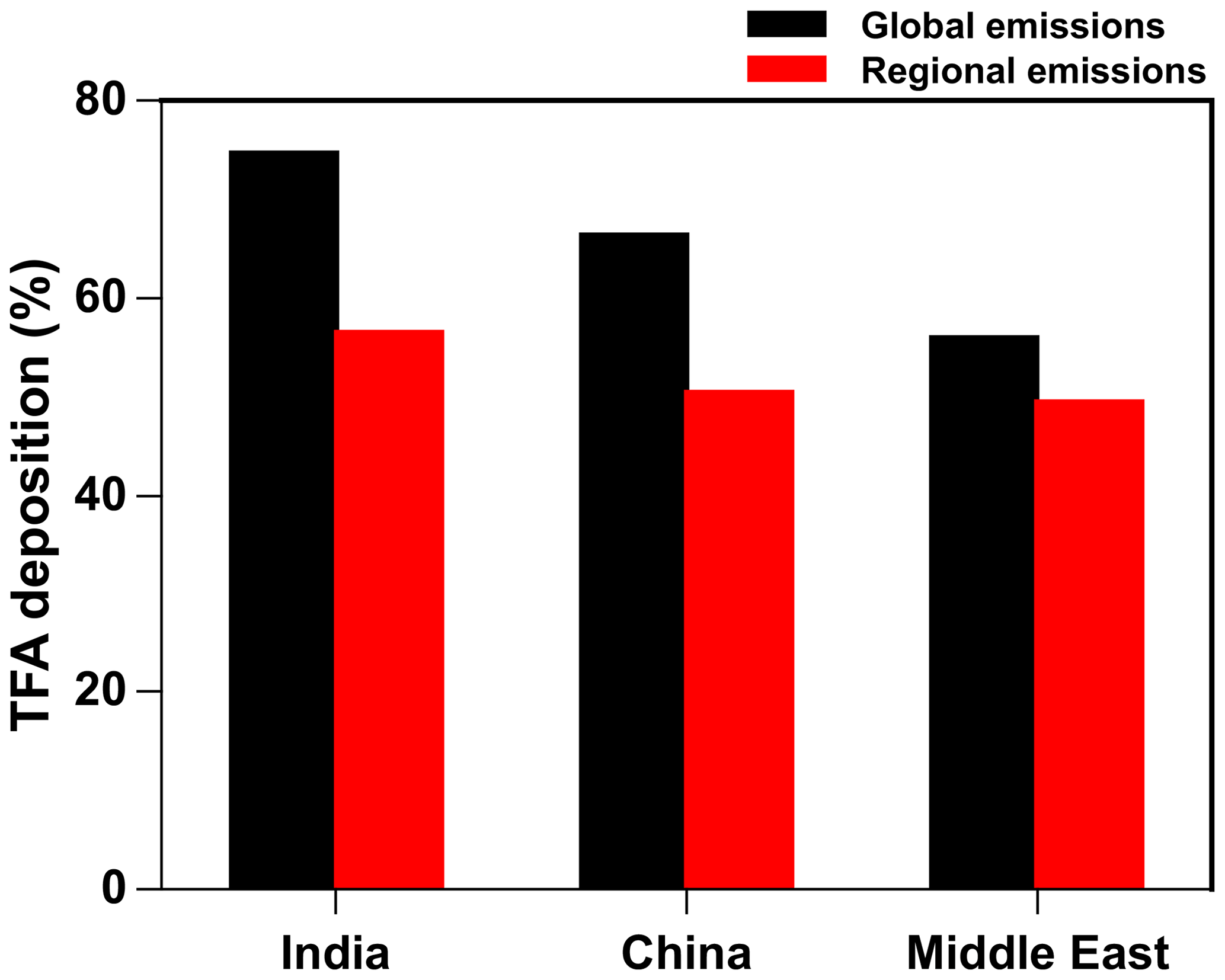
Figure 13Annual percentage of total TFA deposition (dry and wet combined) in India, China, and the Middle East from global and regional (individual regions) emissions.

Figure 14Percentage decrease in TFA deposition (dry and wet combined) by adding Criegee intermediate chemistry to HFO-1234yf emissions over domains in (a) India, (b) China, and (c) the Middle East .
The deposition outside of the region and domains also means that the emitting regions are not the only areas affected by their emission of HFO-1234yf. This is in spite of the relatively short turnover time of HFO-1234yf. (Note that we call this the turnover time because of the way we calculate it in the model.) Since the three countries/regions studied here are adjacent to each other and their domains overlap (Fig. 1), it is possible to estimate the impact of the neighbors' emissions on each other. We consider the emissions over the rest of the world (excluding India, China, the Middle East, the USA, and Europe) from Fortems-Cheiney et al. (2015), assuming HFC-134a is substituted with HFO-1234yf on a mole-per-mole basis (the maximum likely emissions scenario). Figure S13 shows the annual spatial distribution of HFO-1234yf emissions from all the regions as simulated in GEOS-Chem. The percentage deposition of TFA (dry and wet combined) from global and regional (individual regions) emissions of HFO-1234yf is shown in Fig. 13. The TFA deposition increased by 7 %–18 % in the three domains because of the emissions from its neighbors. Figure 13 suggests that, if the entire world switches to HFO-1234yf, the impact of TFA from the near and far neighbors would be noticeable but still be at most a factor of 2 or 3 larger. Figure S14 shows the spatial pattern of the annual total TFA via (a) dry and (b) wet deposition rates from global emissions of HFO-1234yf. The dominant TFA deposition regions were most parts of India, southeastern China, parts of Iran, and the southern Arabian Sea. We discussed, in Sect. 3.5, the potential impacts of such a global switch.
3.8 Reaction of TFA with Criegee intermediates
We examined the influence of the Criegee intermediates (CIs) potential reactions with TFA on its tropospheric levels. We used the CI concentrations in the boundary layer (0–2 km) from Chhantyal-Pun et al. (2017) in GEOS-Chem and simulated the model for 7 months (January to July) using 2015 meteorology. Figure S15 shows the mean surface CI concentration for those 7 months calculated at 2∘ × 2.5∘ spatial resolution. The CI concentrations in the three regions of our study were less than 2500 molec. cm−3. We calculated the percentage decrease in total TFA deposition within the three domains by including the CI chemistry. We assumed at all the CI reactions with TFA have the rate coefficient measured for that of CH2OO with TFA, i.e., cm3 molec.−1 s−1. Figure 14 shows the spatial pattern of decrease in total TFA deposition (dry and wet combined) for 7 months by including CI reaction with gas-phase TFA for emissions of HFO-1234yf by (a) India, (b) China, and (c) the Middle East. At most of the locations within the three domains, the decrease in total TFA deposition was <2.5 %. At a few places in southeastern Asia (Fig. 14a), western China (Fig. 14b), and northern Africa (Fig. 14c), the TFA deposition decreased by 7 %–25 %. The decrease in TFA deposition due to CI was 0.03, 0.32, and 0.08 Gg (total for 7 months) for India, China, and the Middle East domains, respectively. Figure S16 shows the percentage decrease in mean surface TFA mixing ratio by including the reaction of CI with TFA following the emissions of HFO-1234yf emissions from (a) India, (b) China, and (c) the Middle East. The decrease in the mean surface TFA mixing ratio is less than 2 % (0.01 ppt). Overall, the impact of CI on TFA deposition mixing ratio was small in the regions of study.
We have investigated TFA formation from emissions of HFO-1234yf, its dry and wet deposition, and its rainwater concentration over India, China, and the Middle East with GEOS-Chem and WRF-Chem models. We estimated the TFA deposition and rainwater concentrations between 2020 and 2040 for four HFO-1234yf emission scenarios. The models were simulated for a year (2015), with additional 2016 simulations to understand the interannual variability. We also simulated the model using global emissions to assess interregional effects on TFA deposition. The main results of the study are summarized below:
-
Using two models at different spatial resolutions helped us assess the variation in model transport, precipitation, and cloud treatment. These variations yield slightly different calculated TFA levels from the emission of HFO-1234yf. Even though there are discernable differences, the overall conclusions are the same and point to this study's robustness.
-
The accuracy of the GEOS-Chem model's ability to calculate wet deposition over the regions of interest was tested by comparing calculated sulfate rainwater concentration with observations. The model reproduces well the multiyear sulfate rainwater concentration (−3 % to −13 % bias) and its spatial variability (R>0.80) in the three domains.
-
Our calculated TFA amounts over the USA, Europe, and China were comparable to those previously reported when normalized to the same emissions.
-
The controlling factor for the amount of TFA from HFO-1234yf is its emissions. The uncertainties in the models and chemistry are secondary to the extent of emissions.
-
The TFA deposition was largest over eastern India, southeastern China, northern Iran, and the southern Arabian Sea. The TFA wet deposition was comparable between the two models.
-
There are large variations in TFA rainwater concentrations associated with rainfall extent. The mean TFA rainwater concentration calculated for the four emission scenarios from GEOS-Chem and WRF-Chem was below the no observable effect concentration (NOEC), suggesting the ecological and human health impacts to be not significant.
-
With a chemical turnover time of HFO-1234yf of 10 d, its impact is not local and extends well beyond the region of emissions. This study highlights the enhanced TFA formation by the simultaneous use of HFO-1234yf by neighboring regions. If all the Northern Hemisphere countries were to use HFO-1234yf, the impact would be higher by a factor of 2 or 3. However, these amounts are still much lower than the NOEC noted above.
-
We estimate that continued use of HFO-1234yf in India, China, and the Middle East are unlikely to lead to detrimental human health effects, based on the current understanding of the effects of TFA in water bodies, as summarized by Neale et al. (2021). (Note that we do not assume the water is treated specifically to remove TFA before consumption.)
-
We note that a hydrology model of the water flow and TFA concentrations in them would be beneficial to quantify the extent of TFA accumulation in pools and flow out to large water bodies.
The GEOS-Chem code is available from https://doi.org/10.5281/zenodo.1464210 (The International GEOS-Chem Community, 2018).
The data that support the findings of this study are available at https://doi.org/10.25675/10217/233938 (David, 2021).
The supplement related to this article is available online at: https://doi.org/10.5194/acp-21-14833-2021-supplement.
ARR designed the study. LMD carried out the GEOS-Chem simulations, and LMD and MB performed the WRF-Chem simulations. LHI, PP, and GJMV provided the emissions data. LMD, MB, and ARR carried out the data analysis. SG extracted information from publications and assembled the data on sulfate deposition. LMD and ARR prepared the paper, with input from all the coauthors. All the authors contributed to the editing of the paper.
The authors declare that they have no conflict of interest.
Publisher's note: Copernicus Publications remains neutral with regard to jurisdictional claims in published maps and institutional affiliations.
We are grateful to Jan Kazil (NOAA/CSL) and Rajesh Kumar (NCAR), for their help with the WRF-Chem. We are thankful to Jared Brewer and Viral Shah, for helping with TFA chemistry in GEOS-Chem. We are thankful to Kirpa Ram, for providing the sulfate rainwater concentration data over India. We are grateful to Anwar Khan, Rabi Chhantyal Pun, Dudley Shallcross, and Andrew Orr-Ewing, for providing their calculated Criegee intermediate concentrations.
This research has been supported by the Global Forum for Advanced Climate Technologies. NCAR is supported by the National Science Foundation (USA). Pallav Purohit and Lena Höglund-Isaksson received funding from IIASA and the National Member Organizations that support the institute.
This paper was edited by Maria Kanakidou and reviewed by two anonymous referees.
Amann, M., Bertok, I., Borken-Kleefeld, J., Cofala, J., Heyes, C., Höglund-Isaksson, L., Klimont, Z., Nguyen, B., Posch, M., Rafaj, P., Sandler, R., Schöpp, W., Wagner, F., and Winiwarter, W.: Cost-effective control of air quality and greenhouse gases in Europe: Modeling and policy applications, Environ. Model. Softw., 26, 1489–1501, https://doi.org/10.1016/j.envsoft.2011.07.012, 2011.
Amos, H. M., Jacob, D. J., Holmes, C. D., Fisher, J. A., Wang, Q., Yantosca, R. M., Corbitt, E. S., Galarneau, E., Rutter, A. P., Gustin, M. S., Steffen, A., Schauer, J. J., Graydon, J. A., Louis, V. L. St., Talbot, R. W., Edgerton, E. S., Zhang, Y., and Sunderland, E. M.: Gas-particle partitioning of atmospheric Hg(II) and its effect on global mercury deposition, Atmos. Chem. Phys., 12, 591–603, https://doi.org/10.5194/acp-12-591-2012, 2012.
Boutonnet, J. C., Bingham, P., Calamari, D., de Rooij, C., Franklin, J., Kawano, T., Libre, J.-M., McCulloch, A., Malinverno, G., Odom, J. M., Rusch, G. M., Smythe, K., Sobolev, I., Thompson, R., and Tiedje, J. M.: Environmental Risk Assessment of Trifluoroacetic Acid, Hum. Ecol. Risk Assess. An. Int. J., 5, 59–124, https://doi.org/10.1080/10807039991289644, 2011.
Burkholder, J. B., Cox, R. A., and Ravishankara, A. R.: Atmospheric Degradation of Ozone Depleting Substances, Their Substitutes, and Related Species, Chem. Rev., 115, 3704–3759, https://doi.org/10.1021/cr5006759, 2015.
Chen, H., Zhang, L., Li, M., Yao, Y., Zhao, Z., Munoz, G., and Sun, H.: Per- and polyfluoroalkyl substances (PFASs) in precipitation from mainland China: Contributions of unknown precursors and short-chain (C2–C3) perfluoroalkyl carboxylic acids, Water Res., 153, 169–177, https://doi.org/10.1016/j.watres.2019.01.019, 2019.
Chhantyal-Pun, R., McGillen, M. R., Beames, J. M., Khan, M. A. H., Percival, C. J., Shallcross, D. E., and Orr-Ewing, A. J.: Temperature-Dependence of the Rates of Reaction of Trifluoroacetic Acid with Criegee Intermediates, Angew. Chem. Int. Edit., 56, 9044–9047, https://doi.org/10.1002/anie.201703700, 2017.
David, L. M.: Dataset associated with “Trifluoroacetic acid depostion from emissions of HFO-1234yf in India, China, and the Middle East”, Colorado State University Libraries [data set], https://doi.org/10.25675/10217/233938, 2021.
David, L. M., Ravishankara, A. R., Kodros, J. K., Venkataraman, C., Sadavarte, P., Pierce, J. R., Chaliyakunnel, S., and Millet, D. B.: Aerosol Optical Depth Over India, J. Geophys. Res.-Atmos., 123, 1–16, https://doi.org/10.1002/2017JD027719, 2018.
David, L. M., Ravishankara, A. R., Kodros, J. K., Pierce, J. R., Venkataraman, C., and Sadavarte, P.: Premature Mortality Due to PM2.5 Over India: Effect of Atmospheric Transport and Anthropogenic Emissions, GeoHealth, 3, 2–10, https://doi.org/10.1029/2018GH000169, 2019.
Duan, Y., Sun, H., Yao, Y., Meng, Y., and Li, Y.: Distribution of novel and legacy per-/polyfluoroalkyl substances in serum and its associations with two glycemic biomarkers among Chinese adult men and women with normal blood glucose levels, Environ. Int., 134, 105295, https://doi.org/10.1016/j.envint.2019.105295, 2020.
Fast, J. D., Gustafson, W. I., Easter, R. C., Zaveri, R. A., Barnard, J. C., Chapman, E. G., Grell, G. A., and Peckham, S. E.: Evolution of ozone, particulates, and aerosol direct radiative forcing in the vicinity of Houston using a fully coupled meteorology-chemistry-aerosol model, J. Geophys. Res.-Atmos., 111, D21305, https://doi.org/10.1029/2005JD006721, 2006.
Fortems-Cheiney, A., Saunois, M., Pison, I., Chevallier, F., Bousquet, P., Cressot, C., Montzka, S. A., Fraser, P. J., Vollmer, M. K., Simmonds, P. G., Young, D., O'Doherty, S., Weiss, R. F., Artuso, F., Barletta, B., Blake, D. R., Li, S., Lunder, C., Miller, B. R., Park, S., Prinn, R., Saito, T., Steele, L. P., and Yokouchi, Y.: Increase in HFC-134a emissions in response to the success of the Montreal protocol, J. Geophys. Res., 120, 11728–11742, https://doi.org/10.1002/2015JD023741, 2015.
Freeling, F., Behringer, D., Heydel, F., Scheurer, M., Ternes, T. A., and Nödler, K.: Trifluoroacetate in Precipitation: Deriving a Benchmark Data Set, Environ. Sci. Technol., 54, 11210–11219, https://doi.org/10.1021/acs.est.0c02910, 2020.
George, C., Saison, J. Y., Ponche, J. L., and Mirabel, P.: Kinetics of mass transfer of carbonyl fluoride, trifluoroacetyl fluoride, and trifluoroacetyl chloride at the air/water interface, J. Phys. Chem., 98, 10857–10862, https://doi.org/10.1021/j100093a029, 1994.
Giglio, L., Randerson, J. T., and Van Der Werf, G. R.: Analysis of daily, monthly, and annual burned area using the fourth-generation global fire emissions database (GFED4), J. Geophys. Res.-Biogeo., 118, 317–328, https://doi.org/10.1002/jgrg.20042, 2013.
Grell, G. A., Knoche, R., Peckham, S. E., and McKeen, S. A.: Online versus offline air quality modeling on cloud-resolving scales, Geophys. Res. Lett., 31, 16117, https://doi.org/10.1029/2004GL020175, 2004.
Grell, G. A., Peckham, S. E., Schmitz, R., McKeen, S. A., Frost, G., Skamarock, W. C., and Eder, B.: Fully coupled “online” chemistry within the WRF model, Atmos. Environ., 39, 6957–6975, https://doi.org/10.1016/j.atmosenv.2005.04.027, 2005.
Guenther, A.: Corrigendum to “Estimates of global terrestrial isoprene emissions using MEGAN (Model of Emissions of Gases and Aerosols from Nature)” published in Atmos. Chem. Phys., 6, 3181–3210, 2006, Atmos. Chem. Phys., 7, 4327–4327, https://doi.org/10.5194/acp-7-4327-2007, 2007.
Guenther, A. B., Jiang, X., Heald, C. L., Sakulyanontvittaya, T., Duhl, T., Emmons, L. K., and Wang, X.: The Model of Emissions of Gases and Aerosols from Nature version 2.1 (MEGAN2.1): an extended and updated framework for modeling biogenic emissions, Geosci. Model Dev., 5, 1471–1492, https://doi.org/10.5194/gmd-5-1471-2012, 2012.
Guo, J., Huang, G., Wang, X., Li, Y., and Lin, Q.: Investigating future precipitation changes over China through a high-resolution regional climate model ensemble, Earths Future, 5, 285–303, https://doi.org/10.1002/2016EF000433, 2017.
Henne, S., Shallcross, D. E., Reimann, S., Xiao, P., Brunner, D., O'Doherty, S., and Buchmann, B.: Future emissions and atmospheric fate of HFC-1234yf from mobile air conditioners in europe, Environ. Sci. Technol., 46, 1650–1658, https://doi.org/10.1021/es2034608, 2012.
Hodnebrog, Ø., Aamaas, B., Fuglestvedt, J. S., Marston, G., Myhre, G., Nielsen, C. J., Sandstad, M., Shine, K. P., and Wallington, T. J.: Updated Global Warming Potentials and Radiative Efficiencies of Halocarbons and Other Weak Atmospheric Absorbers, Rev. Geophys., 58, 1–30, https://doi.org/10.1029/2019RG000691, 2020.
Hurley, M. D., Wallington, T. J., Javadi, M. S., and Nielsen, O. J.: Atmospheric chemistry of CF3CF=CH2: Products and mechanisms of Cl atom and OH radical initiated oxidation, Chem. Phys. Lett., 450, 263–267, https://doi.org/10.1016/j.cplett.2007.11.051, 2008.
IEA: World Energy Outlook 2017, IEA, Paris, available at: https://www.iea.org/reports/world-energy-outlook-2017 (last access: 24 September 2021), 2017.
Janssens-Maenhout, G., Crippa, M., Guizzardi, D., Dentener, F., Muntean, M., Pouliot, G., Keating, T., Zhang, Q., Kurokawa, J., Wankmüller, R., Denier van der Gon, H., Kuenen, J. J. P., Klimont, Z., Frost, G., Darras, S., Koffi, B., and Li, M.: HTAP_v2.2: a mosaic of regional and global emission grid maps for 2008 and 2010 to study hemispheric transport of air pollution, Atmos. Chem. Phys., 15, 11411–11432, https://doi.org/10.5194/acp-15-11411-2015, 2015.
Kanakidou, M., Dentener, F. J., and Crutzen, P. J.: A global three-dimensional study of the fate of HCFCs and HFC-134a in the troposphere, J. Geophys. Res.-Atmos., 100, 18781–18801, 1995.
Kazil, J., McKeen, S., Kim, S. W., Ahmadov, R., Grell, G. A., Talukdar, R. K., and Ravishankara, A. R.: Deposition and rainwater concentrations of trifluoroacetic acid in the united states from the use of hfo-1234yf, J. Geophys. Res., 119, 14059–14079, https://doi.org/10.1002/2014JD022058, 2014.
Khan, M. A. H., Percival, C. J., Caravan, R. L., Taatjes, C. A., and Shallcross, D. E.: Criegee intermediates and their impacts on the troposphere, Environ. Sci. Process. Impacts, 20, 437–453, https://doi.org/10.1039/c7em00585g, 2018.
Kotamarthi, V. R., Rodriguez, J. M., Ko, M. K. W., Tromp, T. K., and Sze, N. D.: Trifluoroacetic acid from degradation of HCFCs and HFCs: A three-dimensional modeling study, J. Geophys. Res., 103, 5747–5758, 1998.
Krishnan, R., Sanjay, J., Gnanaseelan, C., Mujumdar, M., Kulkarni, A., and Chakraborty, S. (Eds.): Assessment of Climate Change over the Indian Region: A Report of the Ministry of Earth Sciences (MoES), Government of India, Springer, Singapore, 2020.
Kuhns, H., Knipping, E., and Vukovich, J.: Development of a united states–mexico emissions inventory for the big bend regional aerosol and visibility observational (bravo) study, J. Air Waste Manage, 55, 677–692, https://doi.org/10.1080/10473289.2005.10464648, 2005.
Kumar, R., Naja, M., Pfister, G. G., Barth, M. C., Wiedinmyer, C., and Brasseur, G. P.: Simulations over South Asia using the Weather Research and Forecasting model with Chemistry (WRF-Chem): chemistry evaluation and initial results, Geosci. Model Dev., 5, 619–648, https://doi.org/10.5194/gmd-5-619-2012, 2012.
Kumar, R., Barth, M. C., Pfister, G. G., Delle Monache, L., Lamarque, J. F., Archer-Nicholls, S., Tilmes, S., Ghude, S. D., Wiedinmyer, C., Naja, M., and Walters, S.: How Will Air Quality Change in South Asia by 2050?, J. Geophys. Res.-Atmos., 123, 1840–1864, https://doi.org/10.1002/2017JD027357, 2018.
Kumar, S., Kachhawa, S., Goenka, A., Kasamsetty, S., and George, G.: Demand analysis for cooling by sector in India in 2027, New Delhi: Alliance for an Energy Efficient Economy, 2018.
Li, M., Zhang, Q., Kurokawa, J.-I., Woo, J.-H., He, K., Lu, Z., Ohara, T., Song, Y., Streets, D. G., Carmichael, G. R., Cheng, Y., Hong, C., Huo, H., Jiang, X., Kang, S., Liu, F., Su, H., and Zheng, B.: MIX: a mosaic Asian anthropogenic emission inventory under the international collaboration framework of the MICS-Asia and HTAP, Atmos. Chem. Phys., 17, 935–963, https://doi.org/10.5194/acp-17-935-2017, 2017.
Liu, H., Jacob, D. J., Bey, I., and Yantosca, R. M.: Constraints from 210Pb and 7Be on wet deposition and transport in a global three-dimensional chemical tracer model driven by assimilated meteorological fields, J. Geophys. Res.-Atmos., 106, 12109–12128, https://doi.org/10.1029/2000JD900839, 2001.
Luecken, D. J., Waterland, R. L., Papasavva, S., Taddonio, K. N., Hutzell, W. T., Rugh, J. P., and Andersen, S. O.: Ozone and TFA impacts in North America from degradation of 2,3,3,3-tetrafluoropropene (HF0-1234yf), A potential greenhouse gas replacement, Environ. Sci. Technol., 44, 343–348, https://doi.org/10.1021/es902481f, 2010.
Myhre, G., Shindell, D., Bréon, F.-M., Collins, W., Fuglestvedt, J., Huang, J., Koch, D., Lamarque, J.-F., Lee, D., Mendoza, B., Nakajima, T., Robock, A., Stephens, G., Takemura, T., and Zhang, H.: Anthropogenic and Natural Radiative Forcing, edited by: Stocker, T. F., Qin, D., Plattner, G.-K., Tignor, M., Allen, S. K., Boschung, J., Nauels, A., Xia, Y., Bex, V., and Midgley, P. M., Cambridge University Press, Cambridge, United Kingdom and New York, NY, USA, 2013.
Neale, R. E., Barnes, P. W., Robson, T. M., Neale, P. J., Williamson, C. E., Zepp, R. G., Wilson, S. R., Madronich, S., Andrady, A. L., Heikkilä, A. M., Bernhard, G. H., Bais, A. F., Aucamp, P. J., Banaszak, A. T., Bornman, J. F., Bruckman, L. S., Byrne, S. N., Foereid, B., Häder, D.-P., Hollestein, L. M., Hou, W.-C., Hylander, S., Jansen, M. A. K., Klekociuk, A. R., Liley, J. B., Longstreth, J., Lucas, R. M., Martinez-Abaigar, J., McNeill, K., Olsen, C. M., Pandey, K. K., Rhodes, L. E., Robinson, S. A., Rose, K. C., Schikowski, T., Solomon, K. R., Sulzberger, B., Ukpebor, J. E., Wang, Q.-W., Wängberg, S.-Å., White, C. C., Yazar, S., Young, A. R., Young, P. J., Zhu, L., and Zhu, M.: Environmental effects of stratospheric ozone depletion, UV radiation, and interactions with climate change: UNEP Environmental Effects Assessment Panel, Update 2020, Photochem. Photobio. S., 20, 1–67, https://doi.org/10.1007/s43630-020-00001-x, 2021.
Neu, J. L. and Prather, M. J.: Toward a more physical representation of precipitation scavenging in global chemistry models: cloud overlap and ice physics and their impact on tropospheric ozone, Atmos. Chem. Phys., 12, 3289–3310, https://doi.org/10.5194/acp-12-3289-2012, 2012.
Pandey, A., Sadavarte, P., Rao, A. B., and Venkataraman, C.: A technology-linked multi-pollutant inventory of Indian energy-use emissions: II. Residential, agricultural and informal industry sectors, Atmos. Environ., 99, 341–352, https://doi.org/10.1016/j.atmosenv.2014.09.080, 2014.
Papadimitriou, V. C., Talukdar, R. K., Portmann, R. W., Ravishankara, A. R., and Burkholder, J. B.: CF3CF=CH2 and (Z)-CF3CF=CHF: Temperature dependent OH rate coefficients and global warming potentials, Phys. Chem. Chem. Phys., 10, 808–820, https://doi.org/10.1039/b714382f, 2008.
Papasavva, S., Luecken, D. J., Waterland, R. L., Taddonio, K. N., and Andersen, S. O.: Estimated 2017 refrigerant emissions of 2,3,3,3-tetrafluoropropene (HFC-1234yf) in the United States resulting from automobile air conditioning, Environ. Sci. Technol., 43, 9252–9259, https://doi.org/10.1021/es902124u, 2009.
Pfister, G. G., Avise, J., Wiedinmyer, C., Edwards, D. P., Emmons, L. K., Diskin, G. D., Podolske, J., and Wisthaler, A.: CO source contribution analysis for California during ARCTAS-CARB, Atmos. Chem. Phys., 11, 7515–7532, https://doi.org/10.5194/acp-11-7515-2011, 2011.
Purohit, P. and Höglund-Isaksson, L.: Global emissions of fluorinated greenhouse gases 2005–2050 with abatement potentials and costs, Atmos. Chem. Phys., 17, 2795–2816, https://doi.org/10.5194/acp-17-2795-2017, 2017.
Purohit, P., Höglund-Isaksson, L., Dulac, J., Shah, N., Wei, M., Rafaj, P., and Schöpp, W.: Electricity savings and greenhouse gas emission reductions from global phase-down of hydrofluorocarbons, Atmos. Chem. Phys., 20, 11305–11327, https://doi.org/10.5194/acp-20-11305-2020, 2020.
Rigby, M., Montzka, S. A., Prinn, R. G., White, J. W. C., Young, D., O'Doherty, S., Lunt, M. F., Ganesan, A. L., Manning, A. J., Simmonds, P. G., Salameh, P. K., Harth, C. M., Mühle, J., Weiss, R. F., Fraser, P. J., Steele, L. P., Krummel, P. B., McCulloch, A., and Park, S.: Role of atmospheric oxidation in recent methane growth, P. Natl. Acad. Sci. USA, 114, 5373–5377, https://doi.org/10.1073/pnas.1616426114, 2017.
Russell, M. H., Hoogeweg, G., Webster, E. M., Ellis, D. A., Waterland, R. L., and Hoke, R. A.: TFA from HFO-1234yf: Accumulation and aquatic risk in terminal water bodies, Environ. Toxicol. Chem., 31, 1957–1965, https://doi.org/10.1002/etc.1925, 2012.
Sadavarte, P. and Venkataraman, C.: Trends in multi-pollutant emissions from a technology-linked inventory for India: I. Industry and transport sectors, Atmos. Environ., 99, 353–364, https://doi.org/10.1016/j.atmosenv.2014.09.081, 2014.
Solomon, K. R., Velders, G. J. M., Wilson, S. R., Madronich, S., Longstreth, J., Aucamp, P. J., and Bornman, J. F.: Sources, fates, toxicity, and risks of trifluoroacetic acid and its salts: Relevance to substances regulated under the Montreal and Kyoto Protocols, J. Toxicol. Env. Heal. B, 19, 289–304, https://doi.org/10.1080/10937404.2016.1175981, 2016.
Terink, W., Immerzeel, W. W., and Droogers, P.: Climate change projections of precipitation and reference evapotranspiration for the Middle East and Northern Africa until 2050, Int. J. Climatol., 33, 3055–3072, https://doi.org/10.1002/joc.3650, 2013.
The International GEOS-Chem Community:geoschem/geos-chem:GEOS-Chem 12.0.3 (Version 12.0.3), Zenodo [code], https://doi.org/10.5281/zenodo.1464210, 2018.
Tilmes, S., Lamarque, J.-F., Emmons, L. K., Kinnison, D. E., Ma, P.-L., Liu, X., Ghan, S., Bardeen, C., Arnold, S., Deeter, M., Vitt, F., Ryerson, T., Elkins, J. W., Moore, F., Spackman, J. R., and Val Martin, M.: Description and evaluation of tropospheric chemistry and aerosols in the Community Earth System Model (CESM1.2), Geosci. Model Dev., 8, 1395–1426, https://doi.org/10.5194/gmd-8-1395-2015, 2015.
Velders, G. J. M., Fahey, D. W., Daniel, J. S., McFarland, M., and Andersen, S. O.: The large contribution of projected HFC emissions to future climate forcing, P. Natl. Acad. Sci. USA, 106, 10949–10954, https://doi.org/10.1073/pnas.0902817106, 2009.
Velders, G. J. M., Fahey, D. W., Daniel, J. S., Andersen, S. O., and McFarland, M.: Future atmospheric abundances and climate forcings from scenarios of global and regional hydrofluorocarbon (HFC) emissions, Atmos. Environ., 123, 200–209, https://doi.org/10.1016/j.atmosenv.2015.10.071, 2015.
Wallington, T. J., Hurley, M. D., Fracheboud, J. M., Orlando, J. J., Tyndall, G. S., Sehested, J., Møgelberg, T. E., and Nielsen, O. J.: Role of excited CF3CFHO radicals in the atmospheric chemistry of HFC-134a, J. Phys. Chem., 100, 18116–18122, https://doi.org/10.1021/jp9624764, 1996.
Wang, Z., Wang, Y., Li, J., Henne, S., Zhang, B., Hu, J., and Zhang, J.: Impacts of the Degradation of 2,3,3,3-Tetrafluoropropene into Trifluoroacetic Acid from Its Application in Automobile Air Conditioners in China, the United States, and Europe, Environ. Sci. Technol., 52, 2819–2826, https://doi.org/10.1021/acs.est.7b05960, 2018.
Wesely, M. L.: Parameterization of Surface Resistances to Gaseous Dry Deposition in Regional-Scale Numerical Models, Atmos. Environ., 23, 1293–1304, https://doi.org/10.1016/S0950-351X(05)80241-1, 1989.
Wiedinmyer, C., Akagi, S. K., Yokelson, R. J., Emmons, L. K., Al-Saadi, J. A., Orlando, J. J., and Soja, A. J.: The Fire INventory from NCAR (FINN): a high resolution global model to estimate the emissions from open burning, Geosci. Model Dev., 4, 625–641, https://doi.org/10.5194/gmd-4-625-2011, 2011.
WMO (World Meteorological Organization)/United Nations Environmental Program (UNEP): Scientific Assessment of Ozone Depletion: 2006, Global Ozone Research and Monitoring Project, 50, 572 pp., Geneva, Switzerland, 2007.
Young, C. J. and Mabury, S. A.: Atmospheric Perfluorinated Acid Precursors: Chemistry, Occurrence, and Impacts, Rev. Environ. Contam. T., 208, 1–109, 2010.