Seasonal and diurnal variations in biogenic volatile organic compounds in highland and lowland ecosystems in southern Kenya

The East African lowland and highland areas consist of water-limited and humid ecosystems. The magnitude and seasonality of biogenic volatile organic compounds (BVOCs) emissions and concentrations from these functionally contrasting ecosystems are limited due to a scarcity of direct observations. We measured mixing ratios of BVOCs from two contrasting ecosystems, humid highlands with agroforestry and dry lowlands with bushland, grassland, and agriculture mosaics, during both the rainy and dry seasons of 2019 in southern Kenya. We present the diurnal and seasonal characteristics of BVOC mixing ratios and their reactivity and estimated emission factors (EFs) for certain BVOCs from the African lowland ecosystem based on field measurements. The most abundant BVOCs were isoprene and monoterpenoids (MTs), with isoprene contributing > 70 % of the total BVOC mixing ratio during daytime, while MTs accounted for > 50 % of the total BVOC mixing ratio during nighttime at both sites. The contributions of BVOCs to the local atmospheric chemistry were estimated by calculating the reactivity towards the hydroxyl radical (OH), ozone (O₃), and the nitrate radical (NO₃). Isoprene and MTs contributed the most to the reactivity of OH and NO₃, while sesquiterpenes dominated the contribution of organic compounds to the reactivity of O₃.

The mixing ratio of isoprene measured in this study was lower than that measured in the relevant ecosystems in western and southern Africa, while that of monoterpenoids was similar. Isoprene mixing ratios peaked daily between 16:00 and 20:00 (all times are given as East Africa Time, UTC+3),​​​​​​​ with a maximum mixing ratio of 809 pptv (parts per trillion by volume) and 156 pptv in the highlands and 115 and 25 pptv in the lowlands during the rainy and dry seasons, respectively. MT mixing ratios reached their daily maximum between midnight and early morning (usually 04:00 to 08:00), with mixing ratios of 254 and 56 pptv in the highlands and 89 and 7 pptv in the lowlands in the rainy and dry seasons, respectively. The dominant species within the MT group were limonene, α-pinene, and β-pinene.

EFs for isoprene, MTs, and 2-Methyl-3-buten-2-ol (MBO) were estimated using an inverse modeling approach. The estimated EFs for isoprene and β-pinene agreed very well with what is currently assumed in the world's most extensively used biogenic emissions model, the Model of Emissions of Gases and Aerosols from Nature (MEGAN), for warm C₄ grass, but the estimated EFs for MBO, α-pinene, and especially limonene were significantly higher than that assumed in MEGAN for the relevant plant functional type. Additionally, our results indicate that the EF for limonene might be seasonally dependent in savanna ecosystems.

1 Introduction

Biogenic volatile organic compounds (BVOCs) are emitted from vegetation during, e.g., plant growth (e.g., Hüve et al., 2007; Aalto et al., 2014; Taipale et al., 2020), reproduction (e.g., Andersson et al., 2002; Wright et al., 2005), and for defense (Niinemets, 2010; Holopainen and Gershenzon, 2010; Faiola and Taipale, 2020). The reactions of BVOCs with the hydroxyl radical (OH), nitrate radical (NO₃), and ozone (O₃; Schulze et al., 2017; Ng et al., 2017) contribute to the oxidation capacity of the atmosphere (e.g., Mogensen et al., 2015), produce less volatile compounds which can form and growth atmospheric clusters (Matsunaga et al., 2005; Ehn et al., 2014; Kulmala et al., 2004), and impact cloud condensation and scattering of solar radiation, affecting biosphere–atmosphere interactions and local/regional climate change (Claeys et al., 2004; Peñuelas and Staudt, 2010; Sporre et al., 2019; Fig. 1).

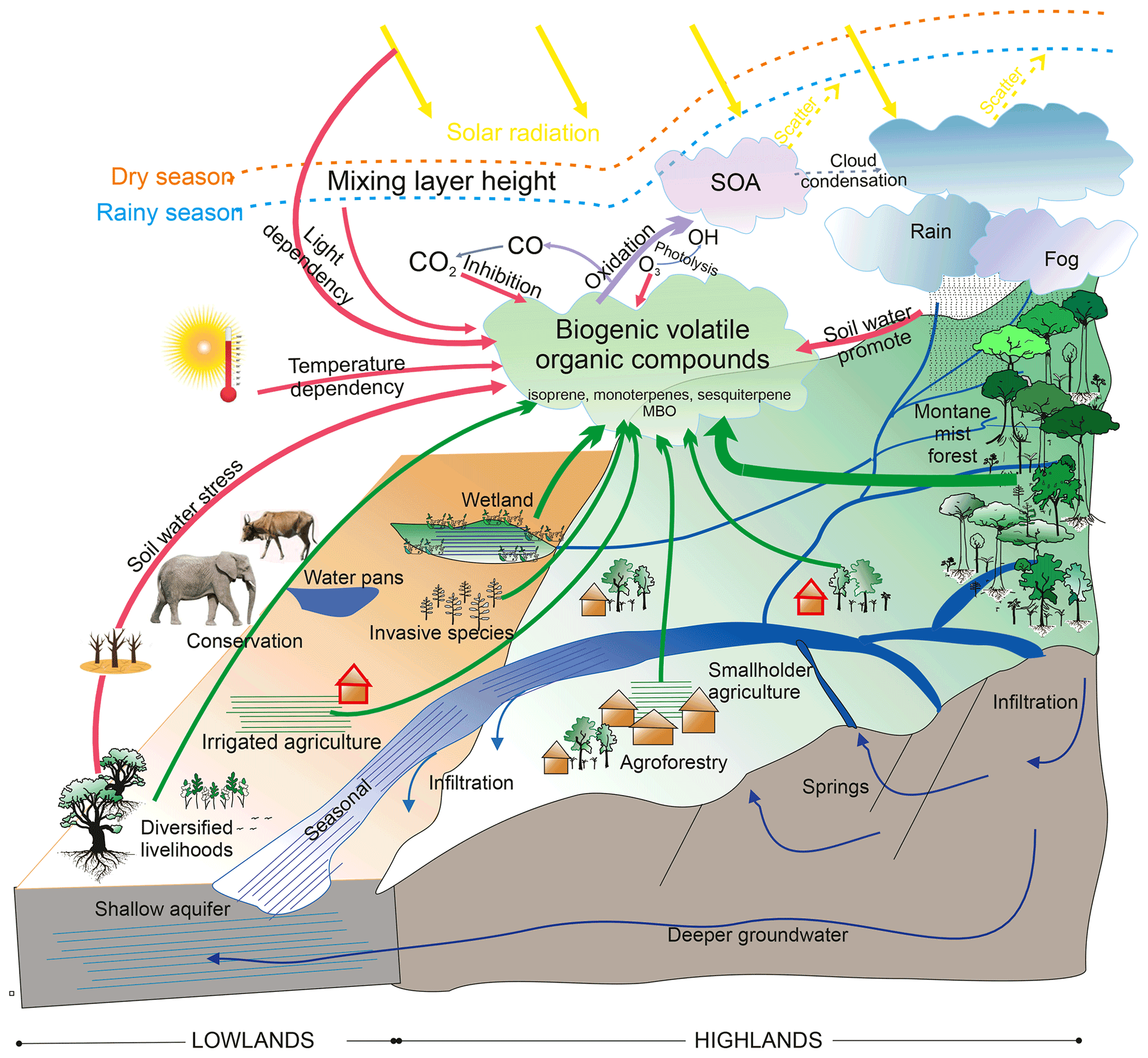
Figure 1 Atmospheric oxidation and abiotic effects on biogenic volatile organic compounds (BVOCs) in African highland and lowland ecosystems. The ecosystem impacts on CO₂ concentration (e.g., photosynthesis and respiration) are not shown in the figure above. SOA is secondary organic aerosol, and OH is hydroxyl radical. The green arrows indicate BVOC sources from African ecosystems. BVOC oxidation and products are shown as purple arrows. The dashed yellow and purple arrows mean BVOC indirect impact to the climate. The abiotic effects on BVOC emissions are shown as red arrows. Blue arrows mean rivers and groundwater. The environments of our study areas are shown as the red house symbols. Figure courtesy of Gretchen Gettel, IHE Delft Institute for Water Education, and Yang Liu and Petri Pellikka, University of Helsinki.

Climate change affects BVOC emissions and oxidation through environmental conditions (Fig. 1; red arrows). Isoprene emissions are known to be both temperature and light dependent (Guenther et al., 1991, 1993; Wildermuth and Fall, 1996; Niinemets et al., 2004) and have been identified as the main contributor to increasing global BVOC levels in response to global warming (Peñuelas and Staudt, 2010). Besides temperature and light, the emission of isoprene depends on soil water availability and thus responds to soil water stress (Guenther et al., 2012). The emission of monoterpenes is known to mainly be controlled by temperature, but the emission of certain monoterpenes (e.g., ocimene) depends greatly on the availability of light (Jardine et al., 2015; Guenther et al., 2012; Loreto et al., 1998). Mochizuki et al. (2020) estimated that monoterpene emissions will increase by 15 % with a 1 ^∘C increase in air temperature due to climate warming. The emission of certain monoterpenes is promoted by increasing soil moisture (Schade et al., 1999; Greenberg et al., 2012) and a decline in moisture-limited conditions (Bonn et al., 2019). Similar to isoprene and monoterpenes, 2-Methyl-3-buten-2-ol (MBO) has shown that its emission is sensitive to light, temperature, and water stress (Gray et al., 2003). Increasing atmospheric carbon dioxide (CO₂) and air pollution (e.g., O₃) are also abiotic factors which affect BVOC emissions negatively or positively (Velikova, 2008; Masui et al., 2021). Since climate variability is rising (Seneviratne et al., 2012), the emission of monoterpenes and isoprene is becoming more variable. This effect becomes especially pronounced in ecosystems that are vulnerable to climatic change.

Dryland ecosystems and human-modified systems, including savannas, bushland, grassland, and agroforestry, are more sensitive and vulnerable to ongoing climate change than other ecosystems (IPCC, 2014). It is estimated that around 18 % of global BVOCs are emitted from grass, shrubs, and crops (Guenther, 2013). This estimate is unfortunately connected with a large degree of uncertainty, since BVOC measurements from these ecosystems are rather scarce (e.g., Guenther, 2013). These climate-sensitive ecosystems are widely distributed and cover 55.2 % of tropical Africa (MDAUS BaseVue 2013, 2020), which have high potential on native ecosystem changes (Zabel et al., 2019), e.g., human-modified systems expansion at the expense of grassland and savannas, which can decrease the global BVOC levels (Unger, 2014). However, these aforementioned climate-sensitive ecosystems are also estimated to face a higher frequency of heat waves, hot nights, droughts, and flooding in the future climate (Niang et al., 2014; Kharin et al., 2018), which can promote or inhibit the certain BVOC releases and make BVOC emissions more changeable. Models can simulate certain abiotic effects, for example temperature changes, soil water stress, and CO₂ inhibition, on BVOC emissions from these climate-sensitive ecosystems in current and future climate scenarios through the setting of suitable parameterizations, i.e., emission factors (EFs) and activity factors (Guenther et al., 2012; Emmerson et al., 2020). However, field measurements focusing on volatile organic compounds from African ecosystems are very limited, especially on monoterpenoids (MTs), sesquiterpenes (SQTs), and MBO. Although previous BVOC measurements detected small quantities of MBO from African ecosystems (Jaars et al., 2016; Liu et al., 2021), MBO oxidation is an important source of ozone and hydrogen radicals (Steiner et al., 2007), which are both important oxidants for new particular formation in the local atmosphere (Jaoui et al., 2012; Zhang et al., 2014).

Previous measurements in tropical savannas have mainly focused on isoprene and/or monoterpenes (Guenther et al., 1996; Klinger et al., 1998; Greenberg et al., 1999, 2003; Otter et al., 2002; Harley et al., 2003; Stone et al., 2010; Jaars et al., 2016; Liu et al., 2021; Fig. 1; green arrows) and were measured during the local rainy season (except Jaars et al., 2016), which increases the challenge of BVOC estimation in these climate-sensitive African ecosystems.

Thus, the overall objective of this study was to quantify BVOC mixing ratios in the humid highland dominated by agroforestry, and the dry lowlands with bushland and agriculture mosaic landscapes in Kenya during the rainy and dry season of 2019. We hypothesized significant differences in BVOC mixing ratios between land cover type at the diurnal scale and at season scale. We were interested in the diurnal and the seasonal variation in BVOC mixing ratios, and we estimated EFs for BVOCs to improve the representation of BVOC emissions from African ecosystems in models.

2 Material and methods

2.1 Experimental sites in Taita Taveta County

BVOC mixing ratios and meteorological measurements were set up in Taita Taveta County in southern Kenya. The county consists of dry savannas located in the lowlands, between 500 and 1000 m a.s.l. (above sea level), and highlands ranging from approximately 1100 to 2200 m a.s.l. (Pellikka et al., 2018).

Taita Taveta County has two rainy and two dry seasons annually due to the Intertropical Convergence Zone forming a bimodal rainfall pattern. The first rainy season (often referred to as the long rains) occurs between March and June, while the second rainy season (referred to as the short rains) is between October and December. The two rainy seasons are separated by dry seasons, with a short hot and dry season from January to February and a long cool and dry season from June to September (Ayugi et al., 2016; Wachiye et al., 2020). The highlands receive more rainfall than the lowlands. The annual precipitation is on average 1132 mm in Mgange (1768 m a.s.l.), corresponding to about twice the rainfall received in Voi at 560 m a.s.l. (587 mm; Erdogan et al., 2011). The annual temperature is 18.5 ^∘C at Taita Research Station in the highlands and 22.3 ^∘C in Maktau field site in the lowlands between 2013 and 2021. Both meteorological measurements are managed by the University of Helsinki, Finland. The length of sunlight remains 12 ± 0.5 h through the entire year, with sunrise around 06:00 ± 0.5 h and sunset about 18:00 ± 0.5 h depending on the season (all times are given as East Africa Time, UTC+3).

The experimental sites were set up in the highlands in Wundanyi at Taita Research Station of the University of Helsinki and in the lowlands in the Maktau field site to represent the highland and lowland ecosystems, respectively (Fig. 2). The Taita Research Station (3^∘40^′ S, 38^∘36^′ E; 1415 m) is located in the middle of the Taita Hills on a windward slope. The landscape is characterized by small agricultural fields with a variety of crops, such as maize, beans, avocados, and grass, with small native or exotic forest stands. The measurement station, which is fenced off, is surrounded by agroforestry landscape, with the closest native and exotic forests at 200 m distance. The natural ecosystem of the Wundanyi site is humid montane forest (Pellikka et al., 2009). Broadleaf evergreen trees and lush grass covered the ground layer during the rainy season at the Wundanyi site (Fig. 2b), while part of the leaves were shed from trees and grass was dried out around our instrument during the dry season (Fig. 2c). The Maktau field site (3^∘25^′ S, 32^∘74^′ E; 1056 m) is located in the lowlands in which the natural ecosystem would be Acacia–Commiphora bushland on savanna (Amara et al., 2020). The measurement site is located inside a fenced farm growing maize, cassava, beans, and papaya trees, surrounded by bushland. The soil on this site was not ploughed yet, and the field was not sown or replanted during our rainy season measurements (Fig. 2d). The instrument was positioned near young cassava bush, with a distance of 50 m from the nearest bushland edge. In the dry season, we collected the samples 2 weeks after the maize was harvested, and the dry maize residuals still remained on the ground (Fig. 2e). The bushland surrounding the field was almost leafless during the dry season sampling, while during the rainy season sampling, the new leaves were starting to sprout. The sites were chosen for the following two reasons: (1) they represented typical highland agroforestry and lowland dry agriculture ecosystems with typical bushland and forest cover, and (2) they provided safety and electricity for continuous measurements.

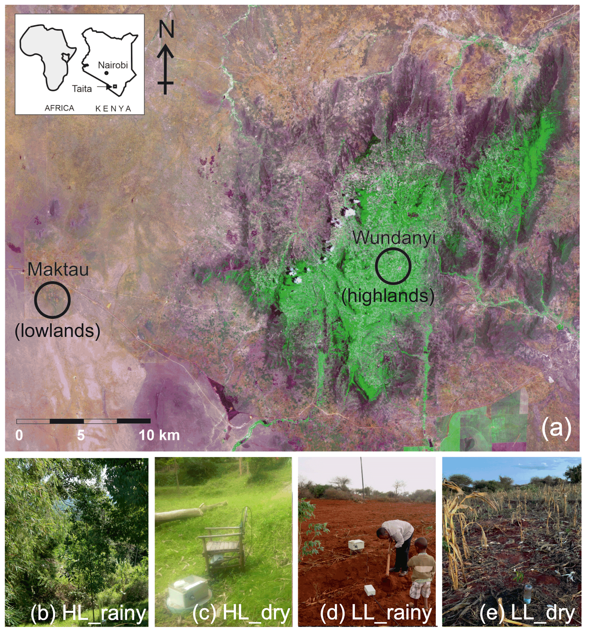
Figure 2 Locations of the highland site (HL) in Wundanyi and the lowland site (LL) in Maktau. The green color in the true color Sentinel satellite image (a) shows the forests and agricultural area in the Taita Hills, while magenta represents grassland with a few fire scars. The brownish areas are areas with less land cover, such as dry bushland, dryland agriculture, and areas used for livestock management. Photographs in panels (b, c, d, e) show the phenological conditions and the surrounding environments of the measurement sites during sampling in the rainy season in April and dry season in September. Photographs by Simon Schallhart, Finnish Meteorological Institute, and Petri Pellikka, University of Helsinki.

2.2 Sample collection and chemical analysis of BVOC mixing ratios

We conducted four campaigns, each lasting several days, in the highlands and lowlands during the onset of the hot and long rainy season from 10 to 17 April 2019 and during the cool and long dry season from 1 to 19 September 2019 (Table A1).

The measurements took place upwind of the two sites, away from roads and at least 10 m away from the nearest residential buildings. In total, two autosamplers were used to collect air into thermal desorption sorbent tubes (STS 25; PerkinElmer, Waltham, MA, USA), with a flow rate of 100 cm⁻³ min⁻¹. All tubes were filled with Tenax TA (60–80 mesh; Sigma-Aldrich, St. Louis, MO, USA) and Carbopack B (60–80 mesh; Sigma-Aldrich, St. Louis, MO, USA). Although the cartridges were stored in an ambient temperature during sampling, sorbents used in the tubes were hydrophobic, and therefore, water was not accumulated. In addition, tubes were flushed with helium for 5 min with the flow of 50 mL min⁻¹ before desorption and analysis to remove traces of humidity.

The sampling time was generally 4 h but was only 2 h during the second campaign due to frequent power failures (Table A1). The sampling took place 25 cm above the ground so that flowing water during heavy rainfall events did not disturb the measurements. All samples were stored in the freezer (at approximately −15^∘) after collection (for 1 to 2 weeks) and before analysis (about 2 months). Tubes were stored in a closed box, with ambient temperature and dark inside, during the transportation to the Finnish Meteorology Institute (less than 1 week).

The mixing ratios of isoprene (C₅H₈), MBO (C₅H₁₀O), MTs (C₁₀H₁₆ and C₁₀H₁₈O), SQTs (C₁₅H₂₄), and bornyl acetate (C₁₂H₂₀O) were measured. MTs consisted of α-pinene, β-pinene, limonene, 3Δ-carene, ρ-cymene, camphene, terpinolene, linalool, and 1,8-cineol. SQTs consisted of longicyclene, iso-longifolene, β-caryophyllene, β-farnesene, and α-humulene. All samples were analyzed in the laboratory of the Finnish Meteorological Institute. An automatic thermal desorption device (PerkinElmer TurboMatrix 650) was connected to a gas chromatograph (PerkinElmer Clarus 600) with a DB–5MS column (50 m × 0.25 mm, film 0.5 µm) and a mass-selective detector (PerkinElmer Clarus 600T). We desorbed all sample tubes at 300 ^∘C for 5 min before cryo-focusing the samples in a Tenax TA cold trap (−30 ^∘C) and injecting them into the column by rapidly heating the cold trap to 300 ^∘C. The method, including potential losses, has been described in detail in Helin et al. (2020). The analytical uncertainties and the limit of quantification are shown in Table A2.

Standards in methanol solutions were used to calibrate the MBO, MTs, and SQTs. We injected the standards into the sampling tubes and flushed away the methanol for 10 min before the analysis. The gaseous calibration standard (National Physical Laboratory) was applied for isoprene. Calibration samples were analyzed together with real samples.

2.3 Complementary measurements and oxidant estimation

2.3.1 Meteorological data

Meteorological data were measured simultaneously with sampling of BVOCs at Taita Research Station and Maktau Weather Station. Hourly air temperature (CS215, Campbell Scientific, UK), relative humidity (CS215, Campbell Scientific, UK), precipitation (ARG100, EML, UK), wind speed, and direction (Taita – wind monitor 05103, R. M. Young​​​​​​​, Traverse City, MI, USA; Maktau – 03002-L wind sentry set, R. M. Young, Traverse City, MI, USA) were measured at both stations. All instruments were positioned at 1.5 m above the ground. Atmospheric pressure (CS106 barometric pressure sensor, Vaisala, Finland), photosynthetic photon flux density (PPFD; SKP215 PAR Quantum, Skye Instruments, UK), and soil moisture (CS650 sensor, Campbell Scientific, UK) were additionally measured at Maktau. The PPFD sensor was positioned around 4 m above the ground. Soil moisture was measured at depths of 10 and 30 cm. Root zone soil moisture calculation has been described in Räsänen et al. (2020).

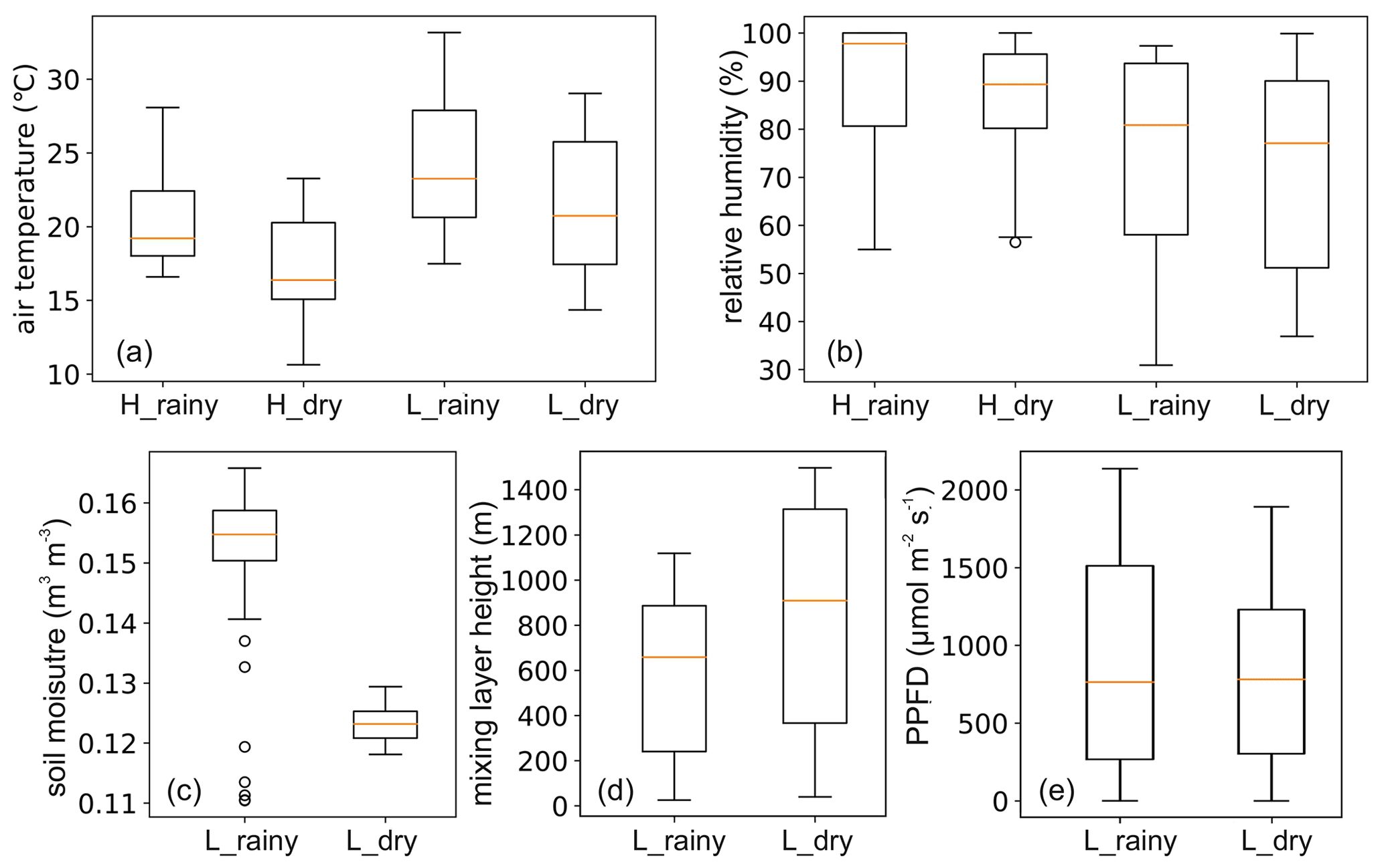
Figure 3 Meteorological measurements in the highland (H) and lowland (L) ecosystems during the rainy and dry seasons. PPFD is photosynthetic photon flux density.

The Chemistry Land–surface Atmosphere Soil Slab (CLASS) model was used to estimate mixing layer heights (MLHs) at the lowland site (Python version; Vilà-Guerau de Arellano et al., 2015). The model initial conditions were derived from the weather station observations. The sensible and latent fluxes from eddy covariance measurements were used as model input. These flux measurements were corrected by conserving the Bowen ratio using the net radiation measurements (Combe et al., 2015). The diurnal MLH data start from 06:00 and continue to 18:00, and the MLHs ranged from 337 ± 25 to 2539 ± 197 m during the rainy season campaign in April and from 361 ± 18 to 2755 ± 146 m during the dry season campaign in September. All meteorology data during BVOC measurements are shown in Fig. 3.

2.3.2 Oxidant concentration estimation

Since the concentrations of oxidants were not measured directly during the campaigns, we used data observed by an Ozone Monitoring Instrument to acquire O₃ column densities to estimate surface O₃ concentrations (the conversion method is described at Ozonesonde, 2021) and ultraviolet B (UVB) radiation intensity to calculate OH radical proxies, using Eq. (1) (Rohrer and Berresheim, 2006; Petäjä et al., 2009).

$$\begin{array}{}\text{(1)}& {\mathrm{OH}}_{\mathrm{proxy}}=\mathrm{5.62}\times {\mathrm{10}}^{\mathrm{5}}\times {\mathrm{UVB}}^{\mathrm{0.62}}.\end{array}$$

The calculated average midday (local noon time) concentrations of O₃ were 31 and 29 ppbv (parts per billion by volume) in the rainy and dry seasons, respectively, while the corresponding concentration of OH was estimated to be 1.2 × 10⁶ and 1.1 × 10⁶ molec. cm⁻³ in the rainy and dry seasons in our study area, respectively.

2.4 Reactivity calculation

Calculating the reactivity of BVOCs gives insight into the relative role of BVOCs in local atmospheric chemistry. The reactivity of BVOCs (R_i,x, where i refers to the BVOC species and x the oxidant species) was calculated by multiplying the mixing ratio of a specific BVOC (i) with the corresponding reaction rate coefficient (k_i,x) of oxidants (including O₃, OH, and NO₃) using Eq. (2).

$$\begin{array}{}\text{(2)}& R_{i,x}={\mathrm{BVOC}}_i\times k_{i,x}.\end{array}$$

The parameter k_i,x was calculated by using the average air temperature during each measurement (calculation equations described in Table A3). All of the reaction rate coefficients used in this study are provided in Table A4.

The atmospheric lifetime (τ) of different BVOCs shows the oxidation speed of a specific compound or compound group in the atmosphere (Eq. 3). We calculated the lifetime of measured BVOCs in relation to O₃ and OH (x), as stated in Table A4.

$$\begin{array}{}\text{(3)}& {\mathit{\tau }}_{i,x}={\displaystyle \frac{\mathrm{1}}{m}}{\sum }_m{\left(k_{i,x}\times {\mathrm{Oxidant}}_x\right)}^{-\mathrm{1}}.\end{array}$$

The amount of measurements in a certain period (m) was used to average over different measurement periods, described hereafter as late night (00:00 to 04:00), early morning (04:00 to 08:00), late morning (08:00 to 12:00), early afternoon (12:00 to 16:00), late afternoon (16:00 to 20:00), and early night (20:00 to 00:00).

2.5 Emission factor estimation

EFs were estimated for isoprene, MBO, and the detected MTs using inverse modeling. In practice, a simple BVOC emissions and chemistry model was developed for this purpose. The model includes an emissions module based on Guenther et al. (2012). The emissions (F_i) of BVOCs (i) are calculated as Eq. (4) as follows:

$$\begin{array}{}\text{(4)}& F_i={\mathit{\gamma }}_i\cdot {\mathrm{EF}}_i,\end{array}$$

where

$${\mathit{\gamma }}_i=C_{\mathrm{CE}}\mathrm{LAI}{\mathit{\gamma }}_{p,i}{\mathit{\gamma }}_{T,i}{\mathit{\gamma }}_{\mathrm{SM}}.$$

The γ_i is an activity factor which accounts for emission responses due to various environmental parameters and phenological conditions. We considered BVOC emission responses due to light (γ_p,i; Eq. 5), temperature (γ_T,i; Eq. 6), and soil moisture (γ_SM; Eq. 7). A value of 0.57 was assigned to the canopy environment coefficient (C_CE; Simpson et al., 1999, 2012; Guenther et al., 2012), while the one–sided leaf area index (LAI, 2020) was kept constant at a value of 1.53 m² m⁻² (April) or 0.3 m² m⁻² (September).

$$\begin{array}{}\text{(5)}& \begin{array}{rl}{\mathit{\gamma }}_{p,i}& =\left(\mathrm{1}-{\mathrm{LDF}}_i\right)+{\mathrm{LDF}}_i\\ & \times C_p\left[\left(\mathit{\alpha }\times \mathrm{PPFD}\right)/\left({\left(\mathrm{1}+{\mathit{\alpha }}^{\mathrm{2}}\times {\mathrm{PPFD}}^{\mathrm{2}}\right)}^{\mathrm{0.5}}\right)\right],\end{array}\end{array}$$

where

$$\begin{array}{c}{\displaystyle }{C}_p=\mathrm{0.0468}\times \exp \left(\mathrm{0.0005}\times \left[P_{\mathrm{24}}-P_{\mathrm{s}}\right]\right)\times {\left[P_{\mathrm{240}}\right]}^{\mathrm{0.6}}\\ {\displaystyle }\mathit{\alpha }=\mathrm{0.004}-\mathrm{0.0005}\ln \left(P_{\mathrm{240}}\right).\end{array}$$

The parameter LDF_i is the light-dependent fraction of the emission of each individual BVOC, and the values are provided in Guenther et al. (2012). P_s is the standard condition for PPFD, averaged over the past 24 h, and was set to 200 µmol m⁻² s⁻¹ (Guenther et al., 2012). P₂₄ and P₂₄₀ are the average PPFD of the past 24 h and the past 240 h, respectively.

$$\begin{array}{}\text{(6)}& \begin{array}{rl}{\mathit{\gamma }}_{T,i}& =\left(\mathrm{1}-{\mathrm{LDF}}_i\right)\times \exp \left({\mathit{\beta }}_i\left(T-T_{\mathrm{s}}\right)\right)+{\mathrm{LDF}}_i\times E_{\mathrm{opt}}\\ & \times \left[C_{T\mathrm{2}}\times {\displaystyle \frac{\exp \left(C_{T\mathrm{1}}\times x\right)}{C_{T\mathrm{2}}-C_{T\mathrm{1}}\times \left(\mathrm{1}-\exp \left(C_{T\mathrm{2}}\times x\right)\right)}}\right],\end{array}\end{array}$$

where

$$\begin{array}{c}{\displaystyle }\begin{array}{rl}{E}_{\mathrm{opt}}& =C_{\mathrm{eo},i}\times \exp \left(\mathrm{0.05}\times \left(T_{\mathrm{24}}-T_{\mathrm{s}}\right)\right)\\ & \times \exp \left(\mathrm{0.05}\times \left(T_{\mathrm{240}}-T_{\mathrm{s}}\right)\right)\end{array}\\ {\displaystyle }x=\left[\left({\displaystyle \frac{\mathrm{1}}{\mathrm{313}+\left(\mathrm{0.6}\times \left(T_{\mathrm{240}}-T_{\mathrm{s}}\right)\right)}}\right)-\left({\displaystyle \frac{\mathrm{1}}{T}}\right)\right]/\mathrm{0.00831}.\end{array}$$

C_eo,i is an emission-class-dependent empirical coefficient for each BVOC in Table 4 in Guenther et al. (2012)​​​​​​​. T_s represents the standard conditions for leaf temperature and is equal to 297 K. T₂₄ and T₂₄₀ are the average leaf temperature of the past 24 h and the past 240 h, respectively. The leaf temperatures were calculated from observed air temperatures (Eqs. 14.2 to 14.6 in Campbell and Norman, 1998). β_i, C_T1,i, and C_T2 are the empirically determined coefficients. We used 230 for C_T2, according to Guenther et al. (2012), and values for β_i and C_T1,i from Table 4 in Guenther et al. (2012).

$$\begin{array}{}\text{(7)}& {\mathit{\gamma }}_{\mathrm{SM},\mathrm{isoprene}}=\left\{\begin{array}{ll}\mathrm{1}& \mathit{\theta }>{\mathit{\theta }}_{\mathrm{l}}\\ \frac{\mathit{\theta }-{\mathit{\theta }}_{\mathrm{w}}}{\mathrm{\Delta }{\mathit{\theta }}_{\mathrm{l}}}& {\mathit{\theta }}_{\mathrm{w}}<\mathit{\theta }<{\mathit{\theta }}_{\mathrm{l}}\\ \mathrm{0}& \mathit{\theta }<{\mathit{\theta }}_{\mathrm{w}}\end{array}\right.,\end{array}$$

where θ is the volumetric water content of soil. ${\mathit{\theta }}_{\mathrm{l}}={\mathit{\theta }}_{\mathrm{w}}+\mathrm{\Delta }{\mathit{\theta }}_{\mathrm{l}}$, θ_w is the wilting point and was set to 0.1 m³ m⁻³ for the Maktau site (Räsänen et al., 2020), while Δθ_l is an empirical parameter which equals 0.04 (Guenther et al., 2012). γ_SM is only applied for the estimation of the emission of isoprene, according to Guenther et al. (2012).

The model's chemistry module consists of the first step in the oxidation of the BVOCs by O₃ and OH using the reaction rate coefficients listed in Table A3. Reactions with NO₃ were omitted because simulations were only carried out using daytime observations. The model takes the following parameters as input: observations of PPFD, air temperature, soil moisture from the Maktau site, estimated leaf temperatures, estimated concentrations of O₃ and OH (Sect. 2.3.2), modeled daytime MLHs (Sect. 2.3.1), and LAI. In the model, the concentration of O₃ is kept constant within a day, while the daily pattern of the OH concentration follows the solar zenith angle.

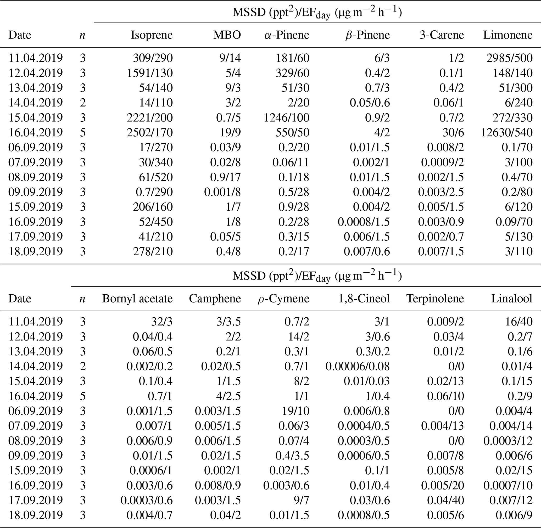
Initial estimations were made for the EFs, and the mixing ratios of the BVOCs were predicted using the model for 1 campaign day at a time. The predicted and measured daytime BVOC mixing ratios were then compared (2–5 data points per day), and the sum of the squared differences between the predicted and observed mixing ratios was calculated for each individual BVOC for each day. A new estimation for the values of the EFs was made, and the process was iterated until a minimum sum of the squared differences was obtained (Table A5). The EF, for each individual BVOC, which led to this minimum value, was considered the most appropriate value for the EF for that particular day (Table A5). Similar simulations were conducted for each measured day. The median values of the estimated EFs during either the rainy or dry season, for each individual BVOC, are our best estimates for the BVOC EFs for the agriculture site located in the savanna ecosystem at Maktau field site. A comparison of the modeled and measured BVOC concentrations, which lead to the minimum sums of the squared differences between the predicted and observed mixing ratios, is provided in Figs. A1 and A2. Similar estimations of EFs were not conducted for the highland site, due to lack of necessary input data to the model.

3 Results and discussion

3.1 Seasonal and diurnal variations of BVOC mixing ratios

For most of the compounds studied, the daily mean mixing ratio was higher during the rainy season than during the dry season. In the highlands, the daily mean isoprene mixing ratio ranged from 134 to 442 pptv in the rainy season and ranged from 36 to 150 pptv in the dry season. The daily mean mixing ratio of MTs was 117 to 233 pptv in the rainy season and was 8 to 75 pptv in the dry season. And that of SQTs was 2 to 30 pptv in the rainy season and 1 to 3 pptv in the dry season. In the lowlands, the daily mean mixing ratios of isoprene ranged from 22 to 69 pptv and from 6 to 15 pptv in the rainy and the dry season, respectively. The mixing ratio of MTs was from 29 to 96 pptv in the rainy season and from 3 to 9 pptv in the dry season. For SQTs, the daily mean mixing ratios ranged from 1 to 2 pptv and was less than 1 pptv in the rainy and the dry season, respectively.

3.1.1 Mixing ratios of isoprene and monoterpenoids

Isoprene and MTs explained over 88 % of the total BVOC mixing ratios of all collected samples, and their mixing ratios in the rainy season were higher than in the dry season in both the highlands and lowlands. The seasonal mean ± standard deviation of the isoprene mixing ratio was 252.2 ± 285 and 66.6 ± 75 pptv in the highlands in the rainy and the dry season, respectively, while the corresponding values were 145.5 ± 73 and 35.2 ± 42 pptv for MTs (Fig. 4). In the lowlands, the mixing ratio of isoprene was 55.3 ± 56 and 11.2 ± 9 pptv in the rainy and the dry season, respectively, while the corresponding values for MTs were 57.8 ± 46 and 4.1 ± 4 pptv. Isoprene and all the MTs showed a clear mixing ratio maximum in the rainy season, and the seasonal mixing ratios of isoprene and MTs remained lower in the lowlands than in the highlands. The temporal variability in measured BVOCs is presented in Fig. A3.

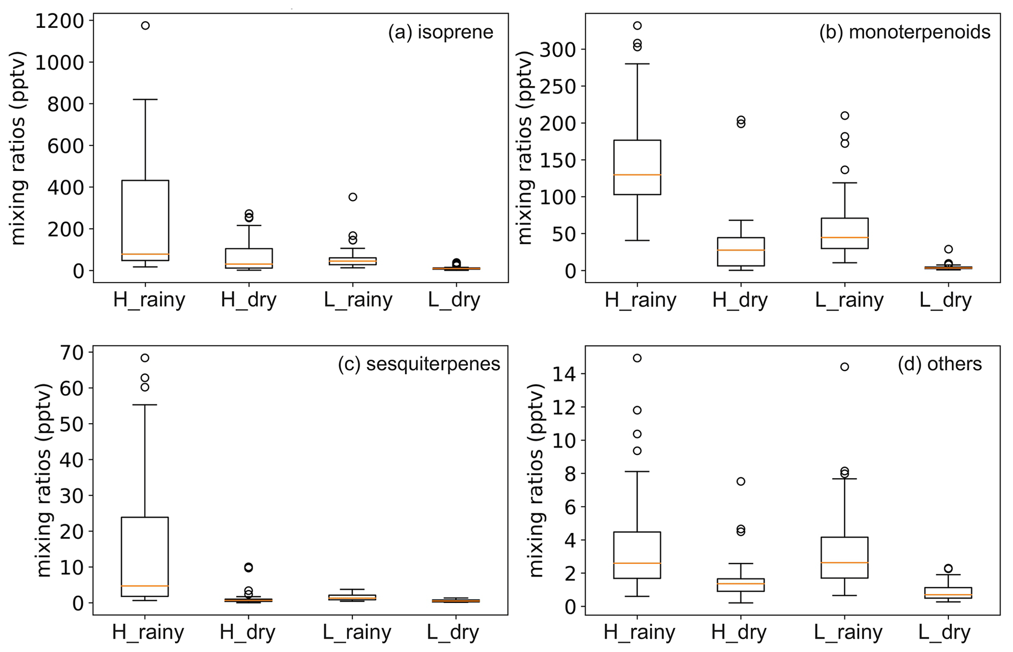
Figure 4 Mixing ratios of isoprene, monoterpenoids, sesquiterpenes, and others (2-Methyl-3-buten-2-ol and bornyl acetate) in the highland and lowland ecosystems during the rainy and dry seasons.

Table 1 LAI, the concentration of ozone, and meteorology conditions detected or estimated in the highland and the lowland sites during the campaigns. Parameters which were not measured in situ are indicated.

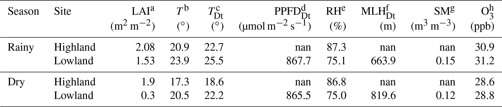
^a LAI – leaf area index (from satellite); ^b T – daily mean ambient temperature; ^c T_Dt – average of daytime (06:00 to 18:00) ambient temperature; ^d PPFD_Dt – daytime mean photosynthetic photon flux density; ^e RH – daily mean relative humidity; ^f MLH_Dt – average of daytime mean mixing layer height (estimated); ^g SM – daily mean soil moisture; ^h O₃ – estimated daily mean concentration of ozone; nan – no observations available; ppb – parts per billion.

Significantly higher temperature, more emitters from different vegetation types, and the lower mixing layer heights were probably the main factors promoting higher mixing ratio during the rainy season (Fig. A4; Table 1). Soil moisture was additionally so low during the dry season (Fig. A5g, h) that it has most probably reduced the emission rate of isoprene. PPFD, RH, and estimated atmospheric oxidant concentrations stayed largely the same during the two seasons and, thus, did not influence the concentration difference. The slightly different PPFD between the two seasons should not have impacted the emission of isoprene, since the light conditions during both seasons were still higher than the saturation point for the production and emission of isoprene (Fig. A5f, m; Guenther et al., 2006). It is likely that the significantly higher LAI in the highlands also caused higher BVOC mixing ratios in the highlands compared to the lowlands. Additionally, the vegetation type in the two ecosystems are different, which might also contribute to the difference, though in which direction is unclear, since emission rates from the particular plant species populating the areas have not been reported so far to our knowledge.

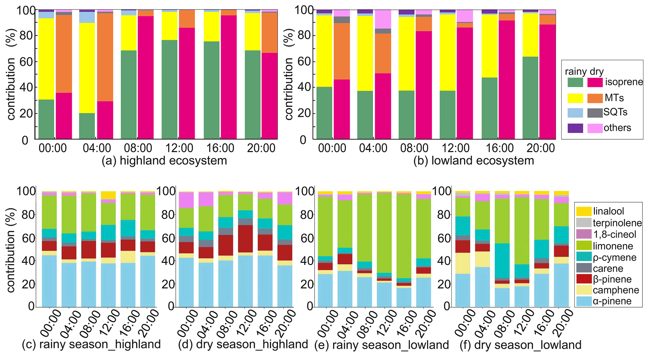
Figure 5 Diurnal contribution of biogenic volatile organic compounds (a, b) and contribution of monoterpenoids (MTs) (c, d, e, f) across the highland site and the lowland site in the rainy and the dry seasons. SQTs is sesquiterpenes, and others are 2-Methyl-3-buten-2-ol and bornyl acetate.

The mixing ratio of isoprene showed distinct diurnal variation in the highlands during both the rainy and dry seasons but in the lowlands only during the dry season (Figs. A6 to A9). The mixing ratio of isoprene increased in the morning, coinciding with sunrise, and stayed high during the rest of the day. The measured mixing ratio of isoprene contributed on average 37 % and 84 % in the highlands and lowlands, respectively, to the total BVOC mixing ratio (Fig. 5).

The mixing ratios of MTs showed higher mixing ratios during night and dark hours than during light hours, particularly during the dry season in both ecosystems (Figs. A6 to A9). Higher mixing ratios of MTs during the night have been observed earlier in savannas in South Africa (Gierens et al., 2014), and a needleleaf forest in California, USA, and Finland (Bouvier-Brown et al., 2009; Hakola et al., 2012). Even though the MT emissions are expected to be highest during daytime, the mixing ratio of MTs is lower since the mixing, and therefore dilution, is highest during daytime and lowest during the night (Mogensen et al., 2011; Hellén et al., 2018).

The diurnal maximum mixing ratio of MTs was on average 254 and 56 pptv in the highlands and 89 and 11.5 pptv in the lowlands in the rainy and the dry seasons, respectively. The diurnal variations in α-pinene and limonene controlled the changes in total MT mixing ratio and contributed over 60 % to the total MT mixing ratio. Decreasing mixing ratios of limonene between day and night led to the diurnal variation in the total mixing ratio of MTs in the rainy season, while decreasing α-pinene controlled the diurnal variation in total MTs in the dry season. The minimum diurnal mixing ratio of MTs occurred in the early night during the rainy season and around noon in the dry season.

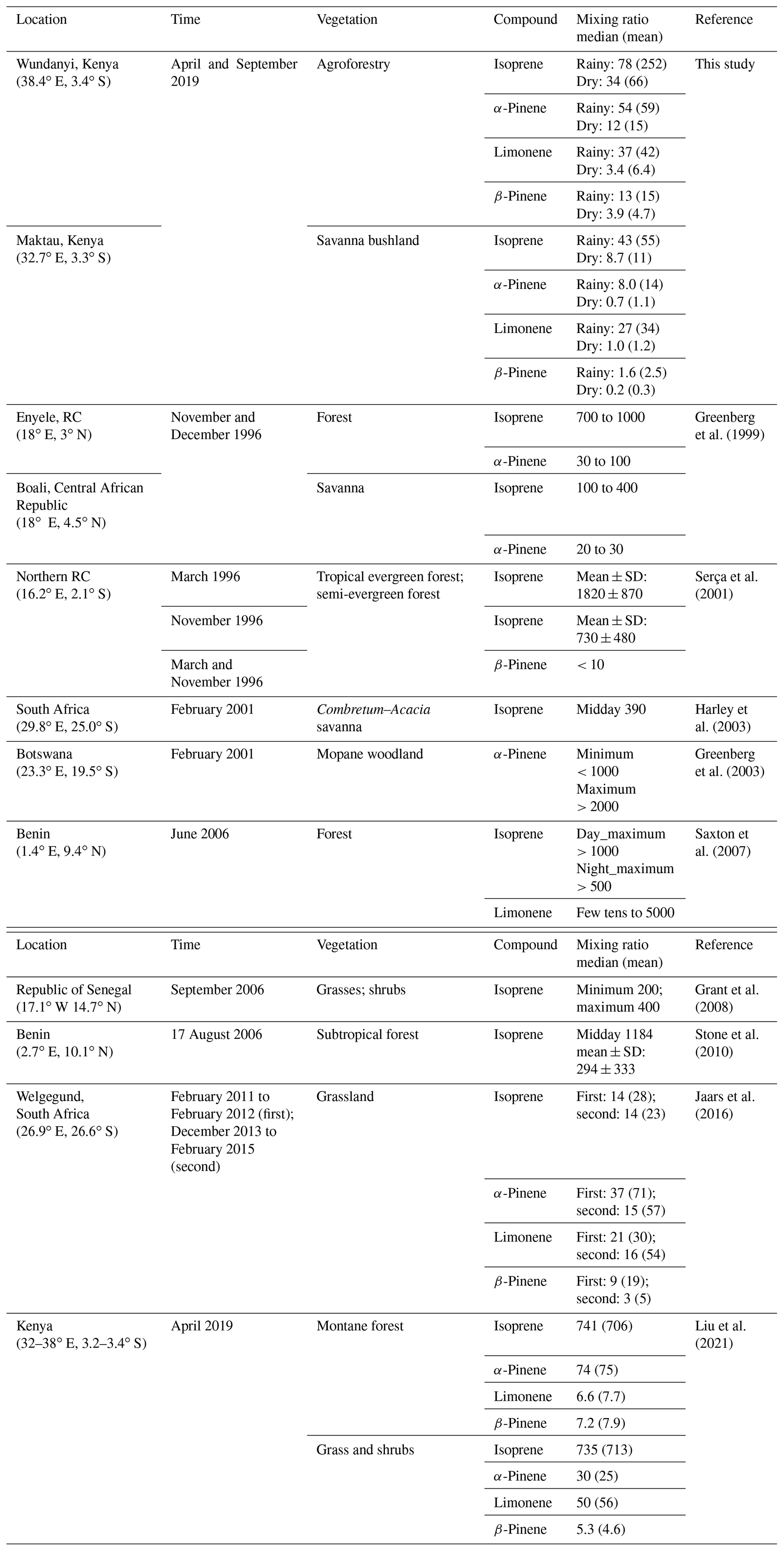
The isoprene mixing ratio ranged from 730 to 1820 pptv in the rainy season of 1996 in a tropical forest in the northern Republic of the Congo (RC), which was covered by evergreen or semi-evergreen trees (Serça et al., 2001). A similar level of isoprene mixing ratio was observed in a forest ecosystem near Enyele, northern RC, with values ranging from 700 to 1000 pptv at the end of the rainy season of 1996 (Greenberg et al., 1999). In western Africa, isoprene mixing ratios of over 1000 pptv during daylight hours were measured in a forest surrounded by a woodland savanna ecosystem in Benin (Saxton et al., 2007). The western African and the two central African measurements aforementioned all showed at least an order of magnitude higher isoprene mixing ratios compared with the measurements in the highlands (Wundanyi) of this study (Table 2). The measured mixing ratios of α-pinene, limonene, and β-pinene in Wundanyi were comparable to the corresponding compound levels from the aforementioned forest measurements. The mixing ratios of isoprene and MTs in Wundanyi are comparable to our previous measurements from three types of montane native forests of the Taita Hills in southern Kenya (Liu et al., 2021). The mixing ratios of isoprene and MTs at the lowland site in Maktau were about 4 times lower than the corresponding levels measured from savanna ecosystems in the Central African Republic (Boali) and South Africa (Greenberg et al., 1999; Harley et al., 2003) and grass and shrubland in western Senegal (Grant et al., 2008) and considerably lower than the corresponding compound levels from woodland in Botswana (Greenberg et al., 2003). The mixing ratios of isoprene and limonene in the rainy season in Maktau are higher than the levels of the corresponding compounds in grassland in Welgegund, South Africa, while the mixing ratios of α-pinene and β-pinene, both in the rainy and the dry seasons, as well as isoprene and limonene in the dry season in Maktau, were lower than the values reported by Jaars et al. (2016). The mixing ratios of α-pinene, limonene, and β-pinene in the rainy season in Maktau were all in the range of the mixing ratios of the corresponding compounds in our previous measurements, while that of isoprene was at lower levels than previously reported (Liu et al., 2021). The differences in mixing ratios between our measurement and from these aforementioned studies could be affected by several factors, e.g., dominant plant species and their distribution, temperature and light, wind speed/direction, mixing layer height, etc. But we were not able to find the key reasons based on the limited details from the other sites.

Table 2 Mixing ratios of biogenic volatile organic compounds in different ecosystems in Africa (mixing ratios are presented as median and mean values, except those with extra explanations (e.g., midday, minimum/maximum, and mean ± SD. The unit of mixing ratios is presented in pptv).

3.1.2 Mixing ratios of sesquiterpenes, MBO, and bornyl acetate

The mixing ratios of SQTs were low and contributed to around 3 % of the total BVOC mixing ratios in all samples. SQTs showed seasonal and diurnal variations similar to those of MTs, but their mixing ratio was much lower than that of MTs, with seasonal mean SQT mixing ratios of 15.0 ± 19 and 1.1 ± 2 pptv in the highlands and 1.5 ± 0.9 and 0.5 ± 0.3 pptv in the lowlands in the rainy and the dry seasons, respectively. SQTs are very reactive, and therefore their contribution to the local atmospheric chemistry can still be significant. The highest daily means were measured during the nighttime, which was the same as in the case of the MTs. β-caryophyllene showed the highest mixing ratios among the SQTs, followed by β-farnesene and/or α-humulene measured in both the rainy and dry seasons. The diurnal trend of β-caryophyllene and β-farnesene followed the variation in total SQTs.

The mixing ratios of MBO and bornyl acetate were both low. MBO explained 2.6 % of the total BVOC mixing ratio of all samples, while bornyl acetate explained 0.5 %. Both compounds have seasonal and diurnal variations. The seasonal mean mixing ratios of MBO and bornyl acetate were 5 and 1.5 times higher in the rainy season than in the dry season in the highlands, respectively, and the mixing ratios of both BVOCs were 6 times higher in the lowlands. The diurnal mean mixing ratios of MBO and bornyl acetate were around 4 and 0.8 pptv in the rainy season in both the highlands and lowlands. MBO mixing ratios were 1 and 0.7 pptv in the dry season in the highlands and lowlands, while that of bornyl acetate was 0.6 and 0.1 pptv, respectively. The daily mean mixing ratio of bornyl acetate was lower than 1 pptv in the rainy and dry seasons both in the highlands and lowlands.

Jaars et al. (2016) measured MBO for the first time in Africa, and they reported that the mean mixing ratios of MBO were 12 and 8 pptv in their first and second campaign, respectively, which are higher than the mean MBO mixing ratios measured in the highlands and lowlands in this study. Guenther (2013) stated that MBO is emitted from most isoprene-emitting vegetation at an emission rate of ∼ 1 % of that of isoprene. The Welgegund data (Jaars et al., 2016) showed that MBO is approximately 30 % of the isoprene mixing ratio, and thus, their study indicated that MBO at Welgegund is most likely from other MBO-emitting species than from isoprene emitters. MBO are higher than 1 % of isoprene mixing ratios in our study, which was 3.7 % and 6.3 % of the isoprene mixing ratio in the highlands in the rainy and dry seasons, respectively, and 7.6 % and 9.8 % in the lowlands. Unfortunately, we could not partition the source of MBO emitter(s) in this study area during our measurements.

Be aware that no measurements were conducted during the short hot (January to February) and short cool (October to December) season, and it is likely that the mixing ratios of BVOCs are different during those seasons than what is presented here due to differences in, e.g., environmental conditions and phenology status.

3.2 Reactivity of the measured BVOCs with oxidants

The reactivity toward O₃, OH, and NO₃ was calculated using the measured BVOC mixing ratios (Fig. 6). The O₃ reactivity of SQTs was 5 to 30 times higher than for other BVOCs, with β-caryophyllene having the highest contribution to the total O₃ reactivity. The strong relative importance of the SQTs compared with other BVOCs for the local O₃ reactivity has also been seen in the ambient air of a Scots pine forest in Finland (Hellén et al., 2018). Out of the total BVOCs, MTs contributed most to the NO₃ reactivity, an average of 13 and 15 times more than isoprene and SQTs, respectively. MTs also contributed to the OH reactivity, with a 0.7 to 1.9 times higher contribution than isoprene during nighttime, while isoprene is the dominant BVOC contributor to the OH reactivity during the day, with 3.1 to 3.5 times higher contributions than MTs.

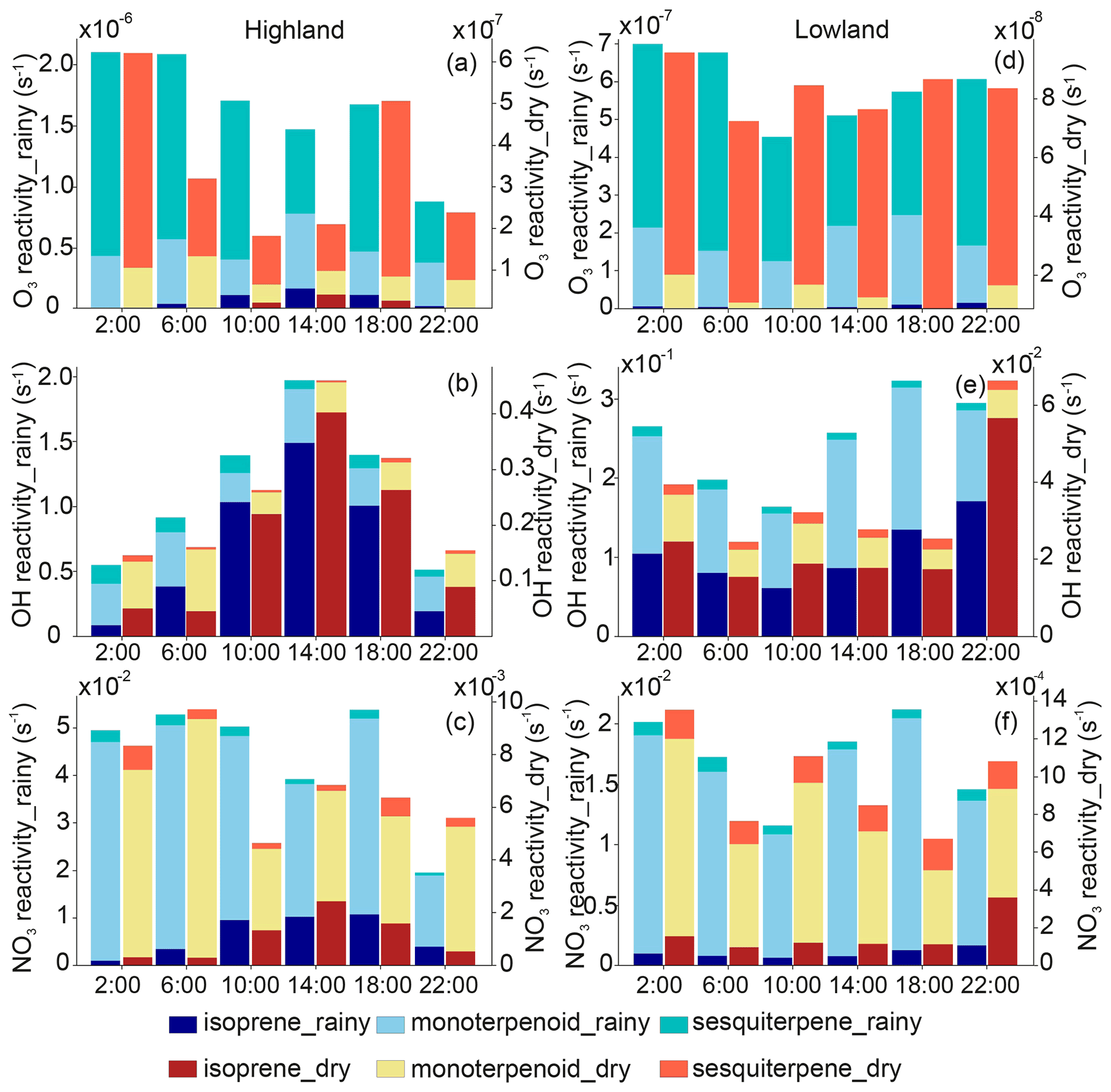
Figure 6 Reactivity of ozone (O₃), hydroxyl (OH), and nitrate (NO₃) of different biogenic volatile organic compounds in the highland (a, b, c) and lowland ecosystems (d, e, f) in the rainy and dry seasons.

Isoprene shows the highest mixing ratio of BVOCs in this study. The atmospheric lifetime of isoprene is 34 and 2.3 h with O₃ and OH, respectively. Following that of isoprene, limonene (∼ 2 h) and α-pinene (∼ 4 h) have higher mixing ratios and are detected to have a relatively short lifetime with OH and O₃ compared with other MTs (except terpinolene and linalool). A higher importance of limonene and α-pinene for OH reactivity than other MTs was also observed in a savanna ecosystem in South Africa (Jaars et al., 2016), which reported that both compounds also had higher mixing ratios than other MTs during their campaigns. Compared with other MTs, limonene has a significantly higher yield for highly oxygenated organic molecules (Ehn et al., 2014; Bianchi et al., 2019), which has been found to be a major component of secondary organic aerosols (e.g., Ehn et al., 2014; Mutzel et al., 2015), for which higher limonene is expected to have a strong impact on local aerosol production in southern Kenya as well. The low mixing ratios of β-caryophyllene and α-humulene have shorter lifetimes with OH and O₃ than other SQTs and BVOCs. The lifetimes of β-caryophyllene and α-humulene are a few minutes with O₃ and about 1 h with OH (Table A4).

3.3 Estimation of BVOC emission factors

The EFs for isoprene, MBO, and detected MTs, for the agriculture savanna ecosystem surrounding the Maktau site, were estimated for the rainy and dry seasons separately (Fig. 7). The median values of the EF for α-pinene, β-pinene, 3Δ-carene, camphene, and limonene (Fig. 7c to g) are higher during the rainy season in April than during the dry season in September, while the median values of the EF for MBO (Fig. 7b) and all other MTs (Fig. 7g) are higher during the dry season than during the rainy season. If the dependency of soil moisture availability on the emission of isoprene is considered, then the EF for isoprene during both the rainy and dry seasons is effectively the same (Fig. 7a). Considering the variability in the estimated EFs for the two different seasons, only the EFs for limonene show no overlap in the indicated error bars (Fig. 7f), which are defined by the minimum and maximum daily estimated EF. Thus, our results suggest that the EF for limonene might be seasonally dependent.

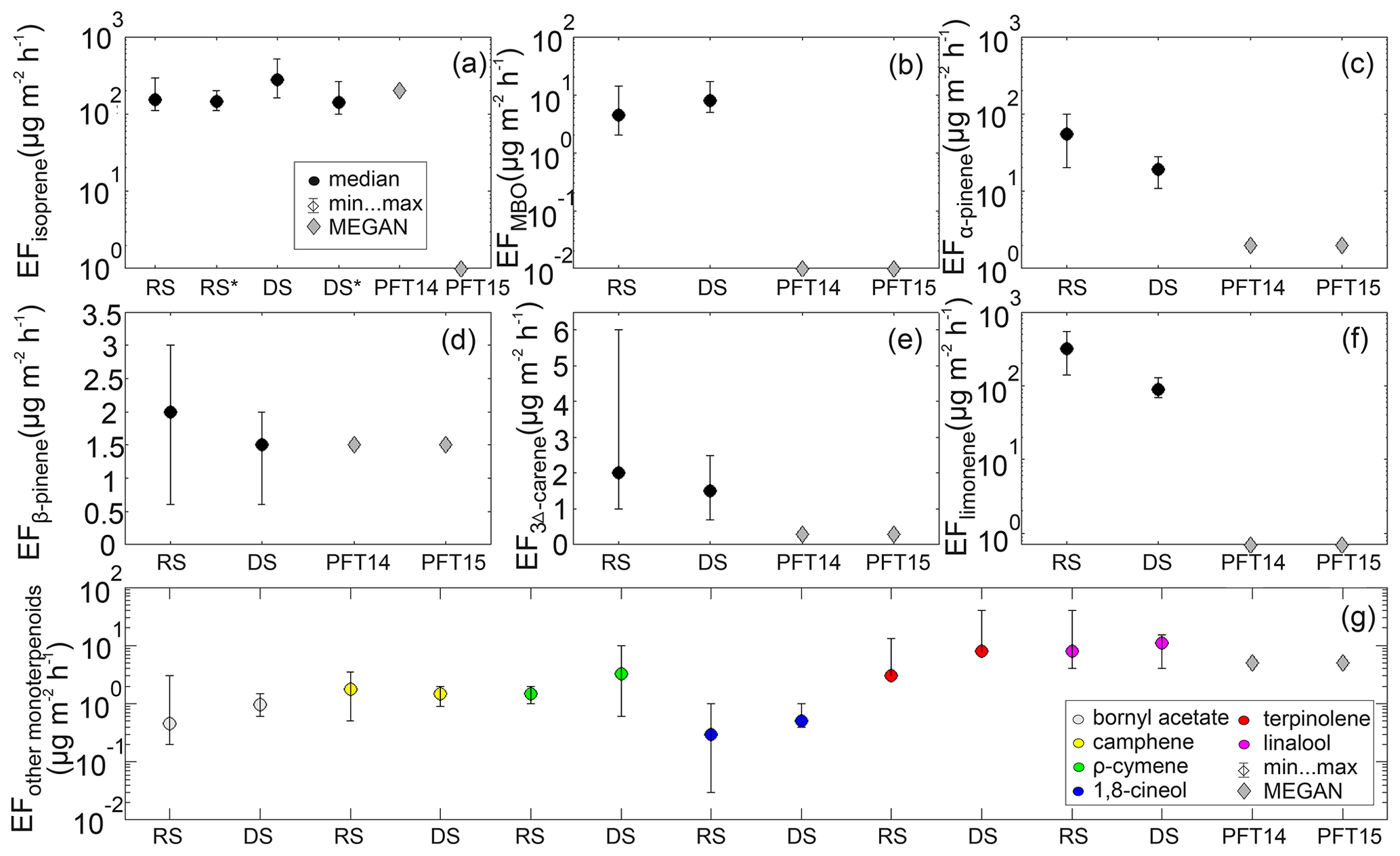
Figure 7 Estimated biogenic volatile organic compound (BVOC) emission factors (EFs) for the agriculture savanna ecosystem surrounding the Maktau field site in comparison with the EFs for warm C₄ grass (PFT14) and Crop1 (PFT15) used in MEGAN v2.1. The EFs have been estimated for the rainy season (RS; April) and for the dry season (DS; September) separately. (a) Isoprene (the EF was estimated by either considering RS or DS or neglecting RS^* or DS^*, which is a dependency of the activity factor on soil moisture availability), (b) 2-Methyl-3-buten-2-ol, (c) α-pinene, (d) β-pinene, (e) 3Δ-carene, (f) limonene, and (g) other monoterpenes, which includes the sum of up to 34 other monoterpenes in MEGAN v2.1 and includes bornyl acetate (gray), camphene (yellow), ρ-cymene (green), 1,8-cineol (blue), terpinolene (red), and linalool (magenta) at Maktau Weather Station. The legend provided in panel (a) is valid for panels (a) to (f).

In order to put the estimated EFs into context and to contribute to an improved representation of BVOC emissions from African ecosystems in models, the estimated EFs are compared with the EFs used in MEGAN v2.1 for warm C₄ grass and Crop1 (Guenther et al., 2012). The estimated EFs for isoprene (155 µg m⁻² h⁻¹ in the rainy season; 280 µg m⁻² h⁻¹ in the dry season) and β-pinene (2 µg m⁻² h⁻¹ in the rainy season; 1.5 µg m⁻² h⁻¹ in the dry season) compare very well with the EFs used in MEGAN for warm C₄ grass (Fig. 7a, d) and, in the case of β-pinene, also for Crop1, since MEGAN assumes the same EF for β-pinene for the two different plant functional types. The estimated median EFs for MBO, α-pinene, 3Δ-carene, and limonene are higher than the EFs used in MEGAN v2.1 by about 8 (4), 17 (53), 1 (2), and 89 (314) µg m⁻² h⁻¹, respectively, where the values in parenthesis are for the rainy season, while the others are for the dry season. The values of the estimated EFs compare best with the EFs allocated for warm C₄ grass in MEGAN in the case of isoprene, α-pinene, β-pinene, and 3Δ-carene compared with the EFs for other plant functional types in MEGAN. However, the estimated EF for limonene is more in line with MEGAN's EF for tropical trees (80 µg m⁻² h⁻¹). Unfortunately, we could not identify the source of the limonene emitter(s). It could be the native African shrubs surrounding the lowland site, which are dominated by acacias (Senegalia mellifera; Vachellia tortilis), but to our knowledge, emission rates have not been reported from these species. The EF for the sum of other MTs (i.e., six MTs at our site and up to 34 in MEGAN) is about 10 and 20 µg m⁻² h⁻¹ higher than that assumed in MEGAN for warm C₄ grass and Crop1 for the rainy and dry seasons, respectively (Fig. 7g). During both seasons, linalool contributes the most to the total EF for the sum of other MTs in this study, while terpinolene accounts for the second-largest fraction. Since the lifetime of monoterpenes is a few hours (see Sect. 3.2), it is likely that part of the detected monoterpenes have been transported to the site from areas covered by other plant functional types than warm C₄ grass and Crop1, such as broadleaved trees and shrubs, which are thought to have a significantly higher potential to emit monoterpenes (Guenther et al., 2012). It is, however, noteworthy that our estimated EF for β-pinene is in line with the listed value by Guenther et al. (2012) for warm C₄ grass and Crop1, but not for broadleaved trees and shrubs, though the lifetime of β-pinene is within the same range as that of the other monoterpenes. The estimated EF for MBO is much higher than that used for C₄ grass in MEGAN. MBO has a lifetime of about half a day, and thus a great part of the detected MBO does not originate from the near vicinity of the site but can have been transported far distances. However, the EF listed in Guenther et al. (2012) for MBO for all plant functional types present in the relevant parts of Africa (Ke et al., 2012) is still about 2–3 orders of magnitude lower than estimated here. This might call for a revision of EFs for MBO, considering that Jaars et al. (2016) also found even higher concentrations of MBO than we did in this study in an area of Africa which also should not contain MBO-emitting species.

We emphasize that the estimated EFs are connected with a large degree of uncertainty, since they are not based on flux measurements from the site but are instead determined using observed BVOC mixing ratios and an inverse modeling approach, which is limited by model assumptions and inputs.

4 Conclusion

In this study we measured mixing ratios of isoprene, MTs, SQTs, bornyl acetate, and MBO in the humid highland and dry lowland ecosystems in Taita Taveta County, southern Kenya, during both a rainy and a dry season.

Isoprene and MTs showed the highest mixing ratios in both the highlands and lowlands, while α-pinene, limonene, and β-pinene accounted for the largest contribution to the total mixing ratio of MTs. Isoprene dominated the total BVOC mixing ratio during daytime and reached diurnal peak mixing ratios in the afternoon in the highlands and in the early evening in the lowlands. The mixing ratio of MTs generally peaked between midnight and early morning, and MTs dominated the total BVOC mixing ratio during nighttime. Isoprene was the dominant BVOC contributor to the OH reactivity, MTs dominated the NO₃ reactivity of BVOCs, and SQTs showed higher contributions to the O₃ reactivity of BVOCs than isoprene and MTs.

Using an inverse model approach with measured BVOC mixing ratios and meteorology data, we estimated the EFs for isoprene, MBO, and MTs in the agriculture savanna ecosystem. The estimated EFs for isoprene and β-pinene agreed very well with what is currently assumed in MEGAN v2.1 for warm C₄ grass, but the estimated EFs for MBO, α-pinene, and especially limonene were significantly higher than what is assumed in MEGAN for the relevant plant functional type. Additionally, our results indicate that the EF for limonene might be seasonally dependent.

Appendix A

Table A1 Sample and flow rate measurements at the Wundanyi station and Maktau field site during the rainy and dry season (sccm – standard cubic centimeters per minute).

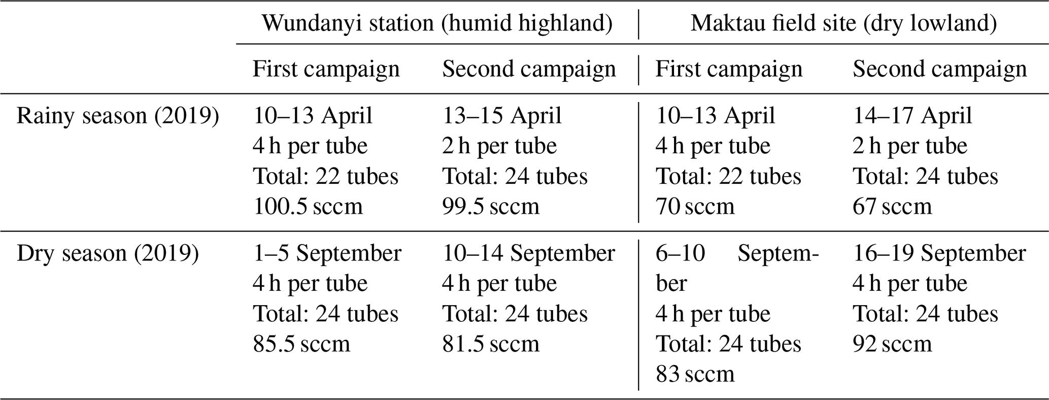
Table A2 The analytical uncertainty (U) for ambient temperature and the limit of quantification (LOQ) for the studied compounds. The estimation method is described in Helin et al. (2020).

Figure A1 Measured and modeled mixing ratios of BVOCs.

Figure A2 Measured and modeled mixing ratios of BVOCs.

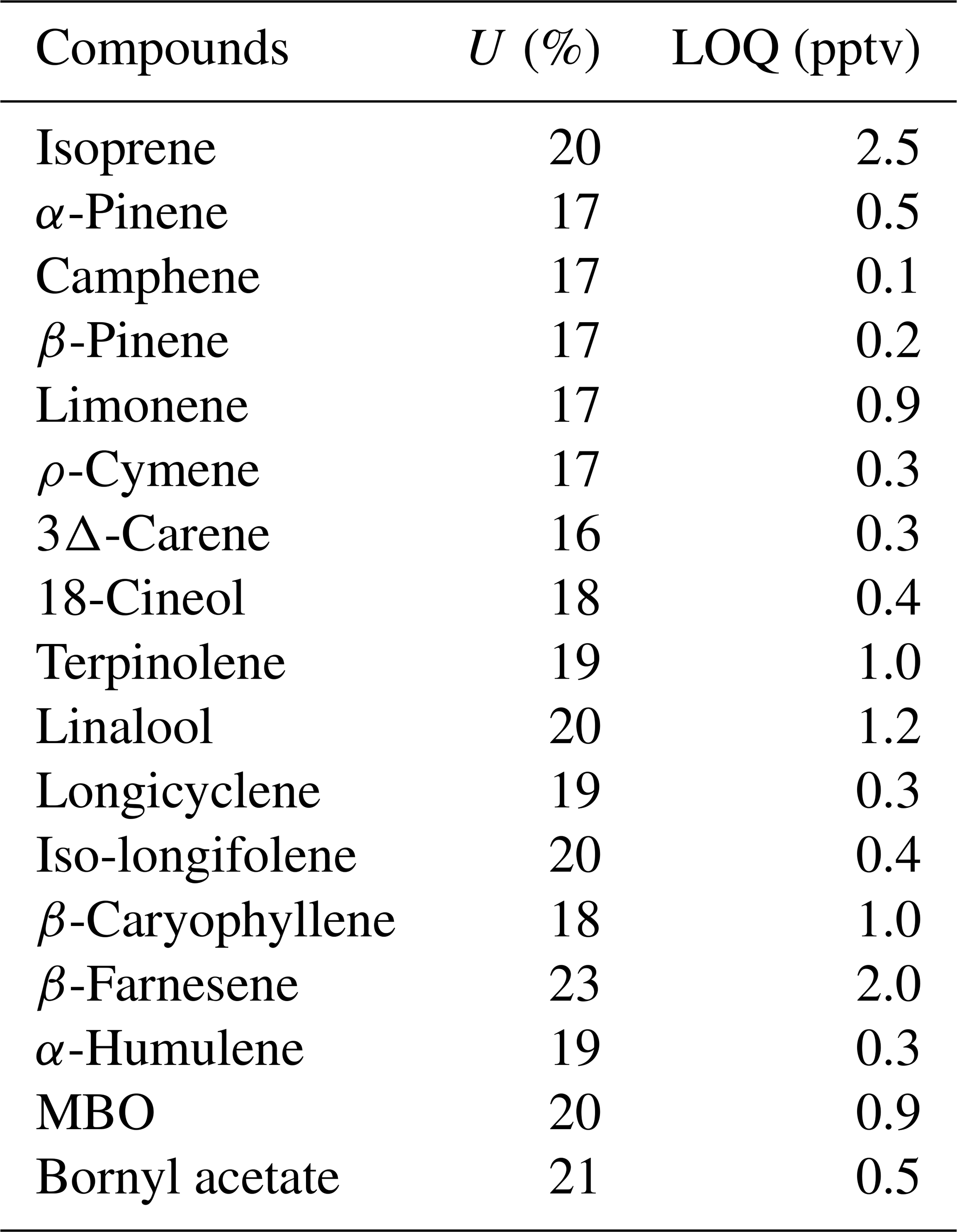
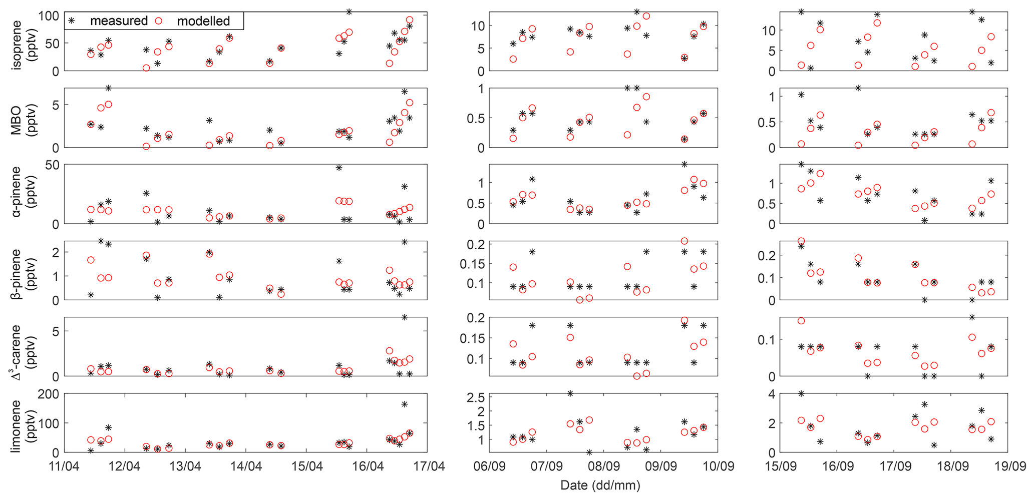
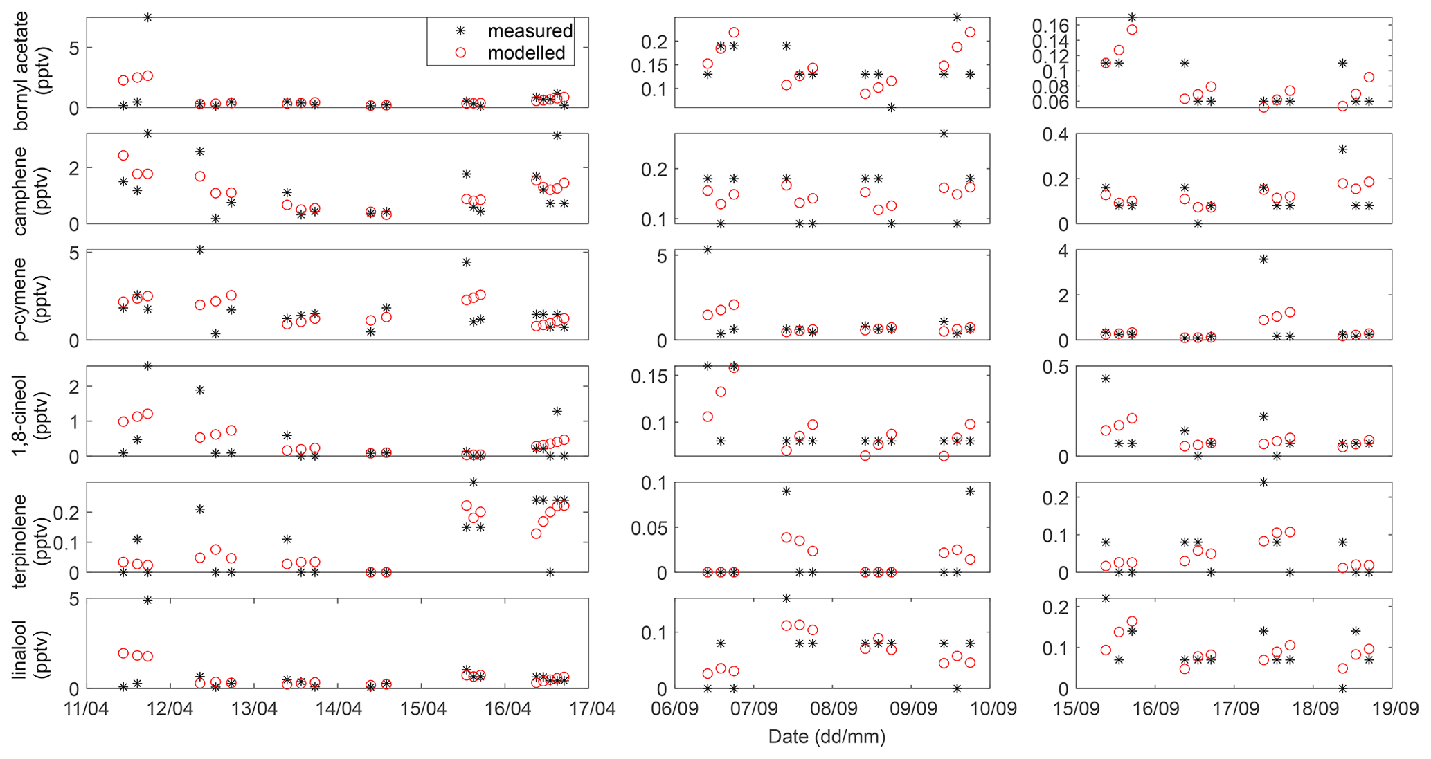
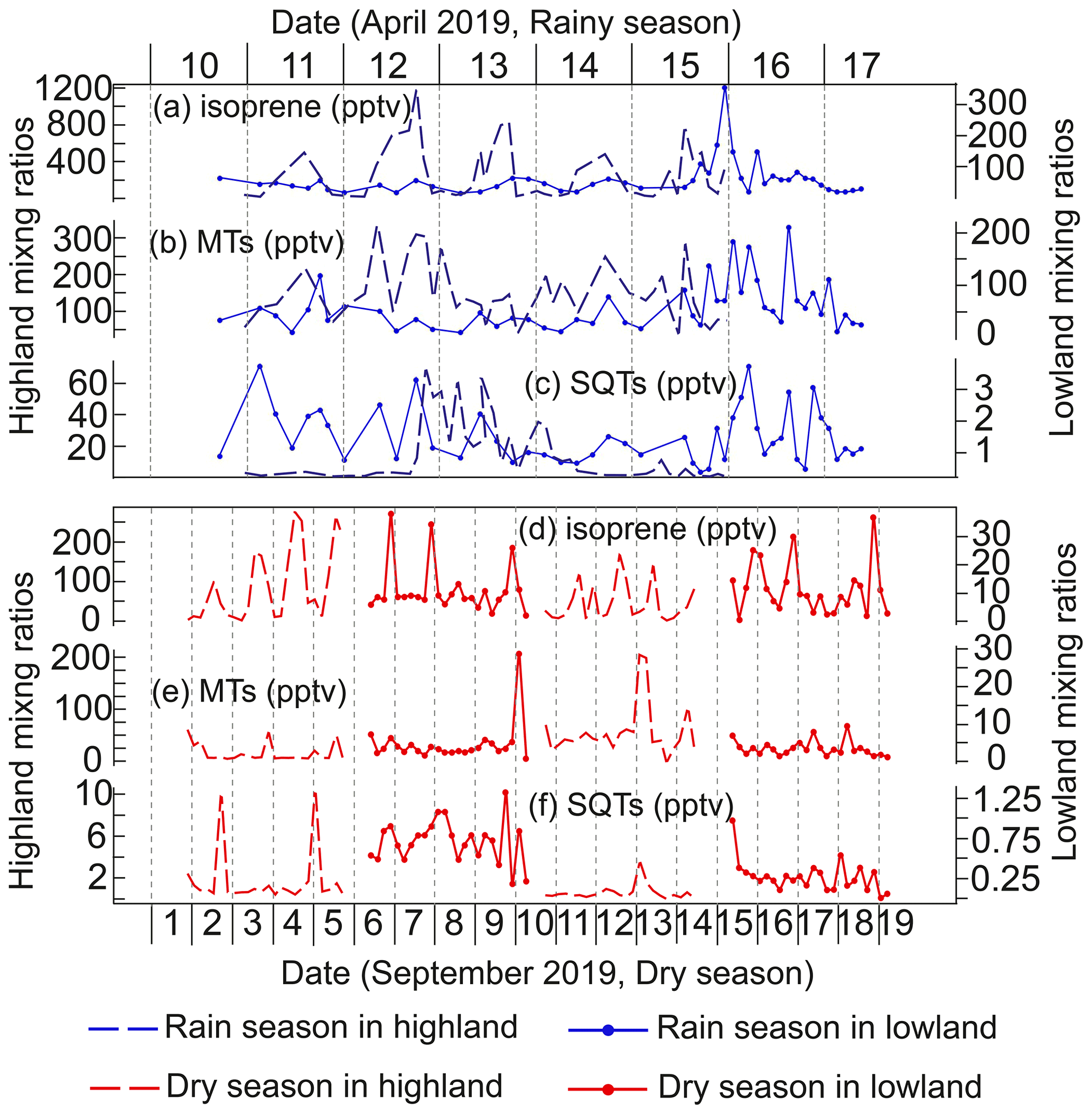
Figure A3 The temporal variability in biogenic volatile organic compound mixing ratios in the highland and lowland ecosystems during the rainy and dry seasons. (a, d) Isoprene. (b, e) Monoterpenoids (MTs). (c, f) Sesquiterpenes (SQTs).

Figure A4 Correlation coefficients between BVOCs and environmental factors.

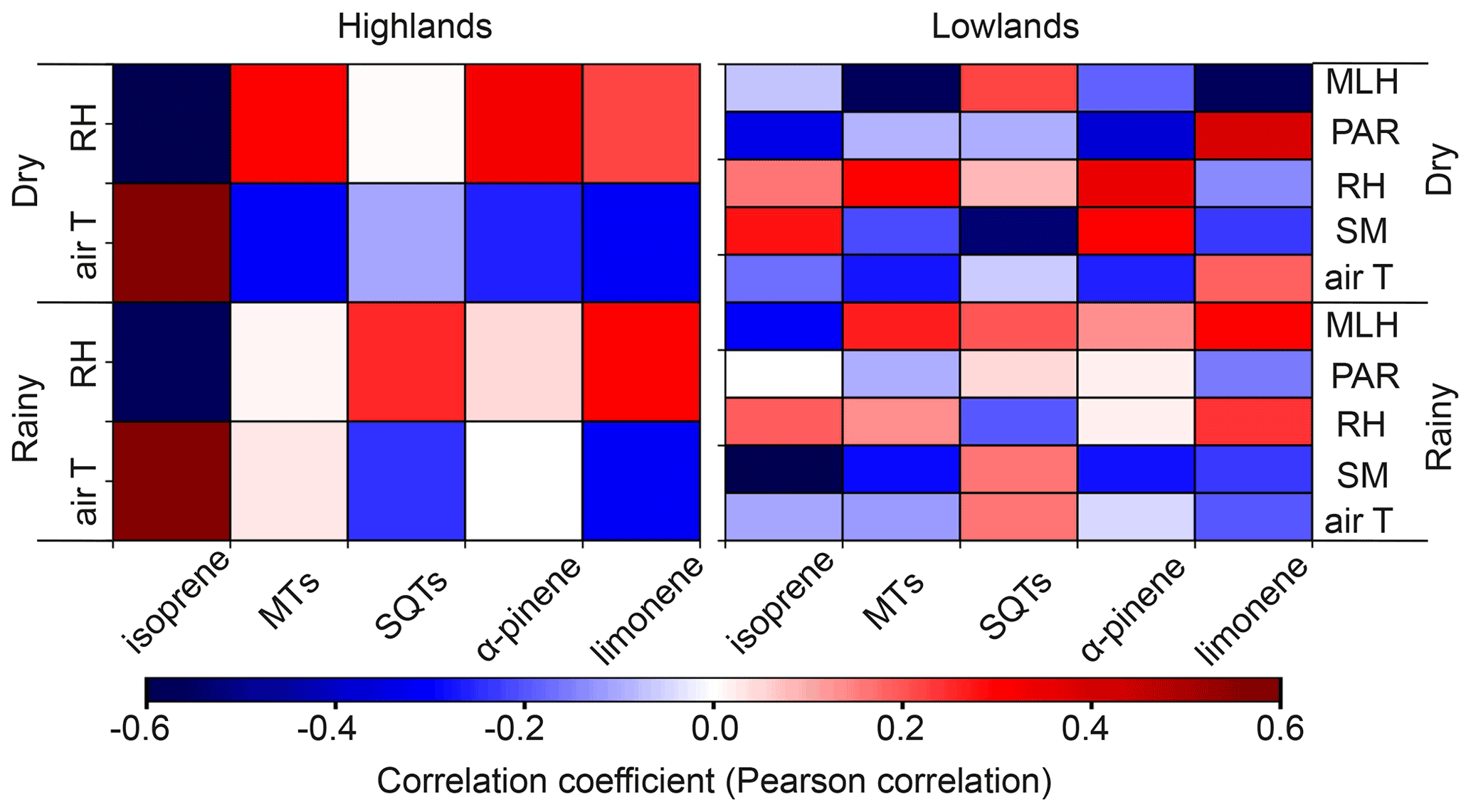
Table A3 Reaction rate coefficients (k_i,x) applied in the model used for estimations of the emission factors and for reactivity calculations. T (K) is air temperature.

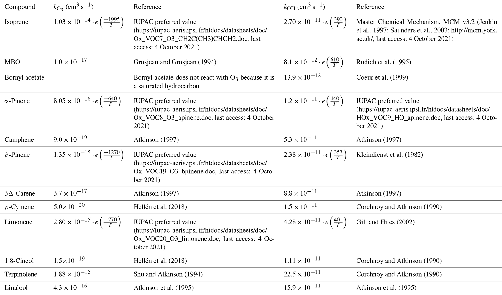
Table A4 Data variation and O₃, OH, and NO₃ reaction rate coefficients (k_i,x; values were shown in daily average) for various BVOCs. RSD is relative standard deviation, units are in percent, the k unit is in cubic centimeters per second (cm³ s⁻¹), and the τ unit is in hours).

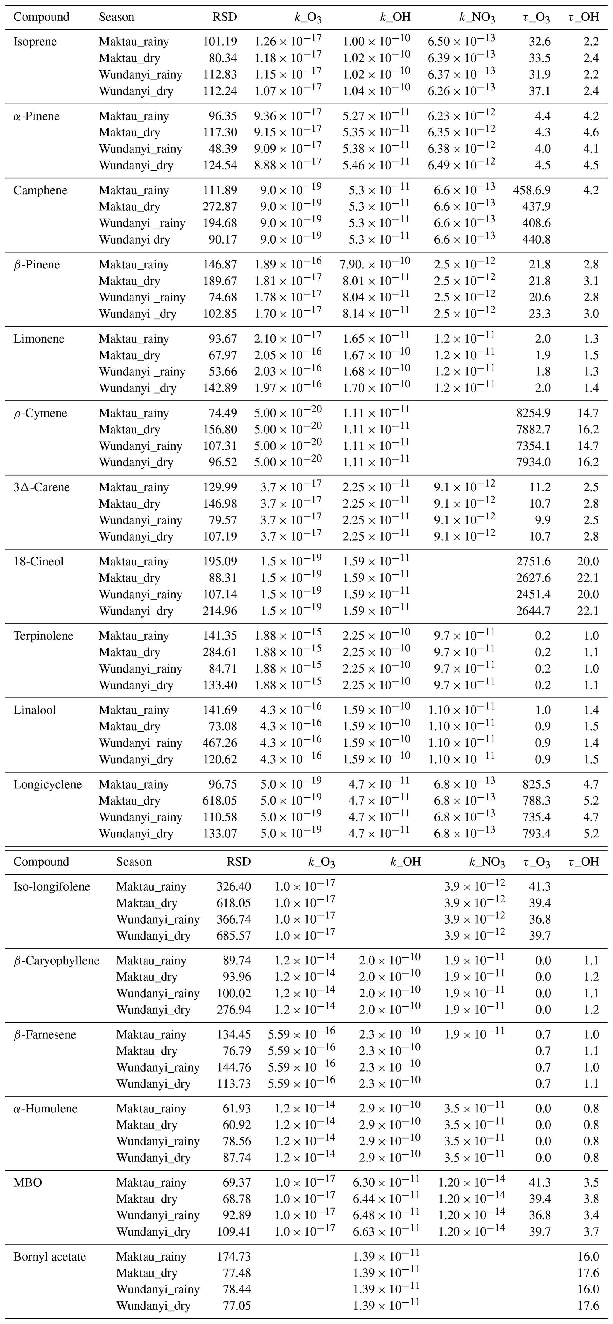
Calculation methods of k values are shown in Table A3.

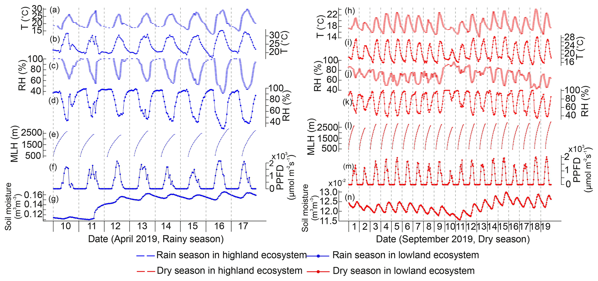
Figure A5 Meteorological measurements in the highland and lowland ecosystems during the rainy and dry seasons. (a, h) Air temperature (T) in the highlands, (b, i) T in the lowlands, (c, j) relative humidity (RH) in the highlands, (d, k) RH in the lowlands, (e, l) mixing layer height (MLH) in the lowlands, (f, m) photosynthetic photon flux density (PPFD) in the lowlands, and (g, n) soil moisture in the lowlands.

Figure A6 BVOC mixing ratios in the highland site during the rainy season. Panels (b) to (f) share the same labels.

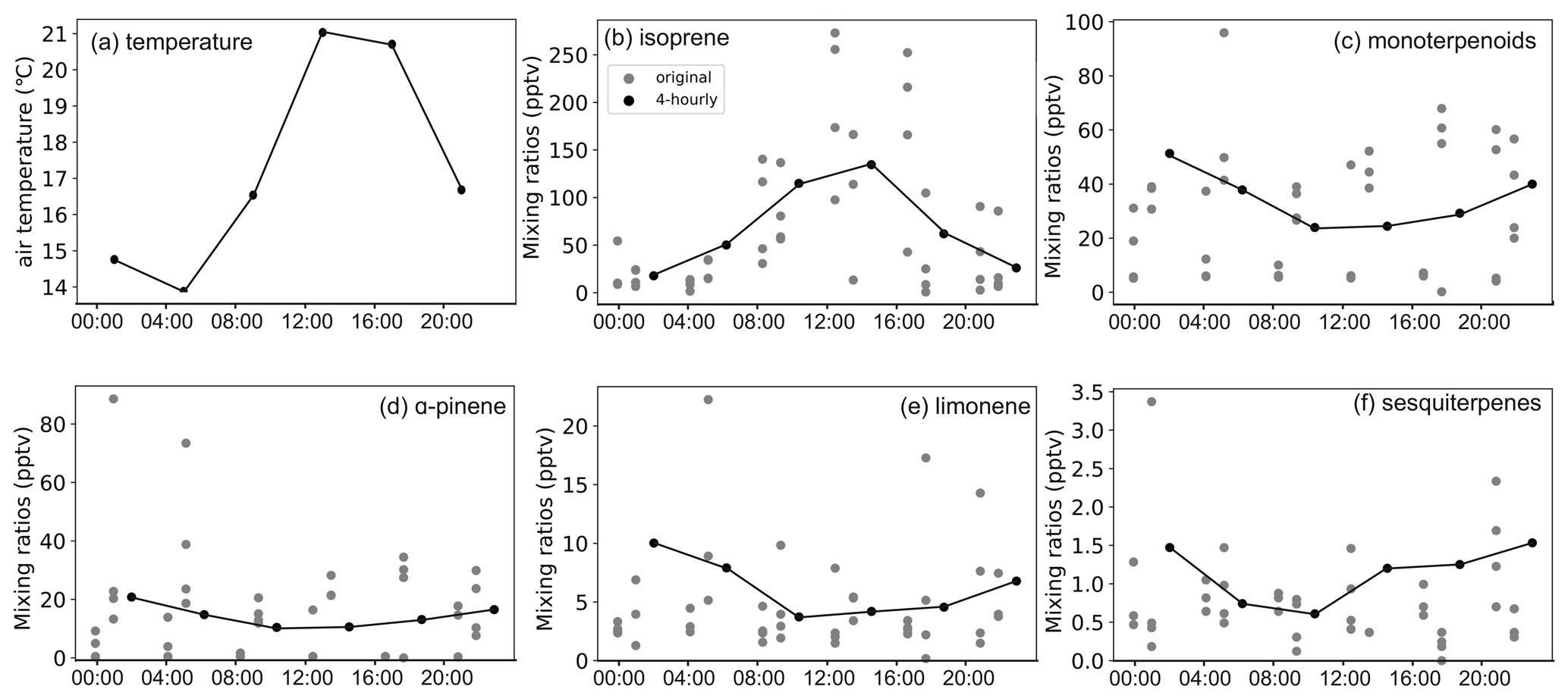
Figure A7 BVOC mixing ratios in the highland site during the dry season. Panels (b) to (f) share the same labels.

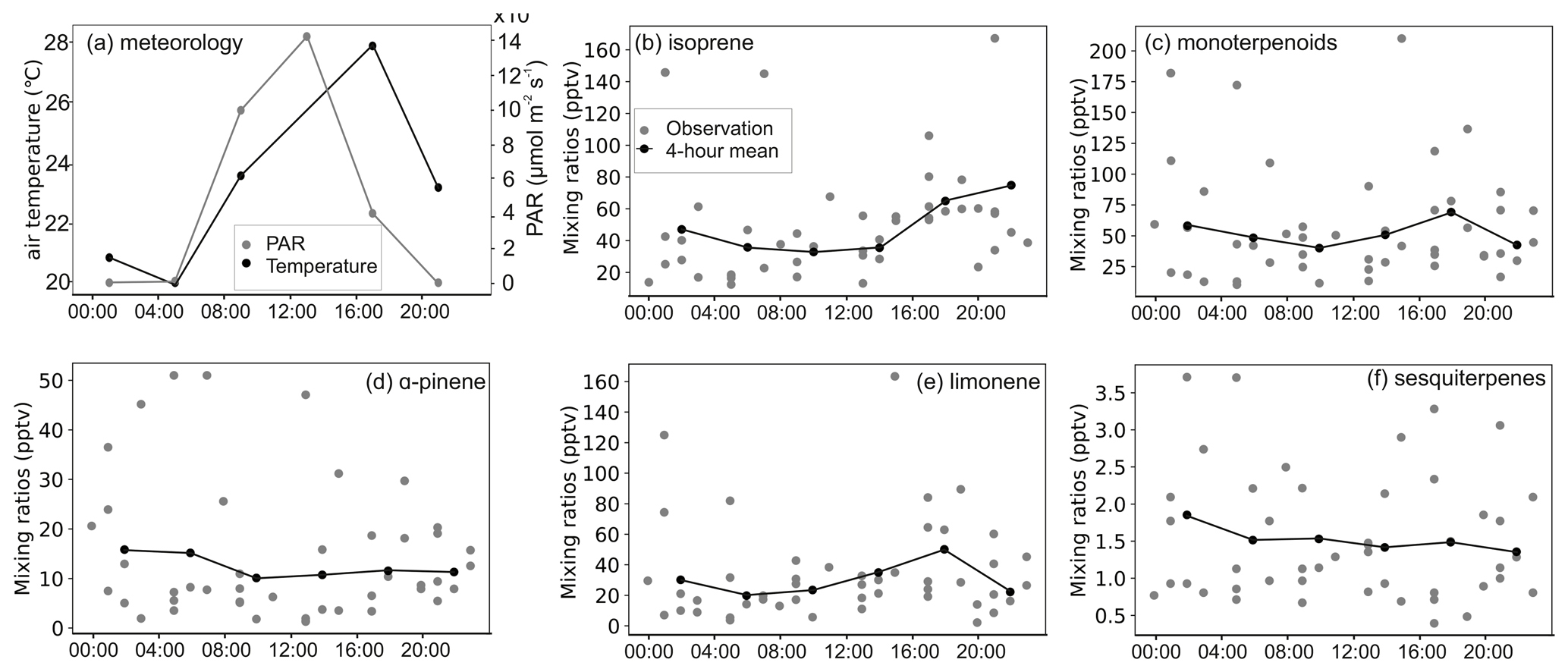
Figure A8 BVOC mixing ratios in the lowland site during the rainy season. Panels (b) to (f) share the same labels.

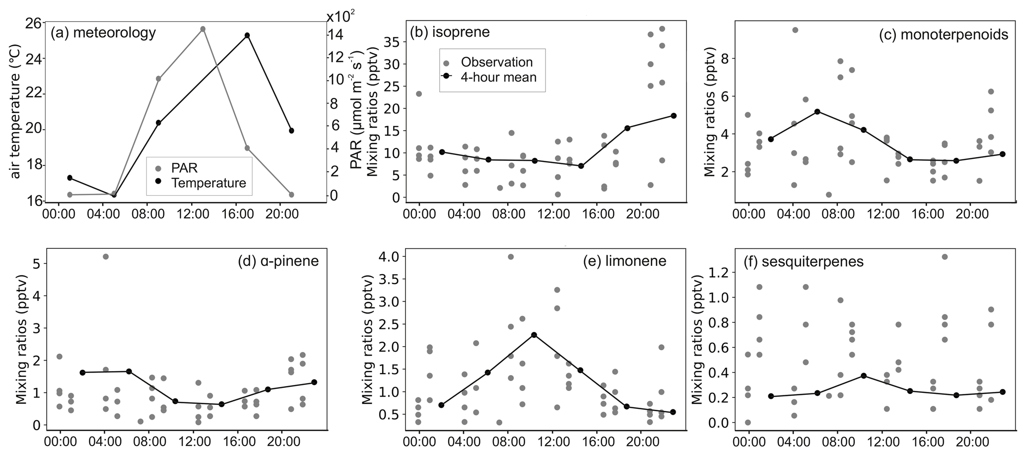
Figure A9 BVOC mixing ratios in the lowland site during the dry season. Panels (b) to (f) share the same labels.

Table A5 Minimum sum of the squared differences (MSSDs) between the predicted and observed volatile organic compound (VOC) mixing ratios for each campaign day presented alongside the emission factor (EF), for each VOC, which is calculated to be the most appropriate value for each day. ${\mathrm{MSSD}}_i=\sum _{j=\mathrm{1}}^n{\left({\left[{\mathrm{BVOC}}_i\right]}_{\mathrm{measurment},j}-{\left[{\mathrm{BVOC}}_i\right]}_{\mathrm{model},j}\right)}^{\mathrm{2}}$, where n is the number of measured VOC mixing ratios samples, and i is the 12 different VOCs for which the mixing ratios were predicted; ppt is parts per trillion, and the date is given as dd.mm.yyyy.​​​​​​​