the Creative Commons Attribution 4.0 License.
the Creative Commons Attribution 4.0 License.
 | 08 Jan 2021
Direct measurements of black carbon fluxes in central Beijing using the eddy covariance method
Rutambhara Joshi
Dantong Liu
Eiko Nemitz
Ben Langford
Neil Mullinger
Freya Squires
James Lee
Yunfei Wu
Xiaole Pan
Pingqing Fu
Simone Kotthaus
Sue Grimmond
Qiang Zhang
Oliver Wild
Michael Flynn
Black carbon (BC) forms an important component of particulate matter globally, due to its impact on climate, the environment and human health. Identifying and quantifying its emission sources are critical for effective policymaking and achieving the desired reduction in air pollution. In this study, we present the first direct measurements of urban BC fluxes using eddy covariance. The measurements were made over Beijing within the UK-China Air Pollution and Human Health (APHH) winter 2016 and summer 2017 campaigns. In both seasons, the mean measured BC mass (winter: 5.49 ng m−2 s−1, summer: 6.10 ng m−2 s−1) and number fluxes (winter: 261.25 particles cm−2 s−1, summer: 334.37 particles cm−2 s−1) were similar. Traffic was determined to be the dominant source of the BC fluxes measured during both seasons. The total BC emissions within the 2013 Multi-resolution Emission Inventory for China (MEIC) are on average too high compared to measured fluxes by a factor of 58.8 (winter) and 47.2 (summer). Only a comparison with the MEIC transport sector shows that emissions are also larger (factor of 37.5 in winter and 37.7 in summer) than the measured flux. Emission ratios of BC ∕ NOx and BC ∕ CO are comparable to vehicular emission control standards implemented in January 2017 for gasoline (China 5) and diesel (China V) engines, indicating a reduction of BC emissions within central Beijing, and extending this to a larger area would further reduce total BC concentrations.
- Article
(8504 KB) - Full-text XML
- BibTeX
- EndNote


Particular matter with a diameter ≤ 2.5 µm (PM2.5) is a major contributor to air pollution (Harrison et al., 1997). It is a global concern given its severe impacts on health, as epidemiological studies identify a variety of cardiovascular and respiratory diseases (Lelieveld et al., 2015; Pope and Dockery, 2006). The daily recommended exposure limit of PM2.5 suggested by the World Health Organisation (WHO) is 25 µg m−3 (Jassen et al., 2012). However, in China concentrations routinely are on the order of 100s µg m−3 (Li et al., 2017; Zhang et al., 2017; Zíková et al., 2016). Black carbon (BC), in general, contributes up to 10 %–15 % of overall PM2.5 and is emitted from incomplete combustion of fossil fuel and biofuel (Seinfeld and Pandis, 1998). Even though its abundance is relatively low in PM2.5, the WHO reports that a 1 µg m−3 increase in BC is associated with greater health risks compared to the same increase in unidentified PM2.5 mass (Jassen et al., 2012). Furthermore, BC is the most optically absorbent aerosol in the atmosphere, with radiative forcing to the climate second only to CO2 (Bond et al., 2013; Ramanathan and Carmichael, 2008). Therefore, reducing BC will potentially have major benefits for both air quality and climate.
The capital of China, Beijing, is well known for its air quality issues, with a large population frequently exposed to unsafe levels of air pollution. Therefore, improving air quality is a priority for government and environmental agencies in China. Ongoing policies targeting reduction in the use of solid fuel domestic cooking and heating (Barrington-Leigh et al., 2019) and introducing traffic management policies and vehicular emission controls (Wu et al., 2017) have been successful in reducing PM2.5 and consequently BC in recent years (Sun et al., 2016). However, Beijing still suffers from severe haze episodes, with BC concentrations frequently 10 times greater than those observed in western countries (Liu et al., 2014; Wu et al., 2016). Therefore, understanding and quantifying BC emission sources can help reach the Chinese government targets for clean air.
Scientists routinely use atmospheric chemistry models to assess local and regional air quality and determine the effectiveness of potential legislative interventions. As air quality models are underpinned by emission inventories, the accuracy of their forecasts is closely coupled to inventory uncertainties from emission factors and activity statistics (e.g. fuel consumption and source) (Cao et al., 2006; Hodnebrog et al., 2014). Such uncertainties are challenging to resolve as the spatial resolution increases up to a few kilometres (Zheng et al., 2017).
In China, sources have rapidly changed with urbanisation and environmental controls. Ground-based measurements of emissions can help to refine and verify emission inventories. For BC, this is complicated by the use of BC ∕ PM2.5 ratios to estimate BC emissions. This ratio is highly variable depending on fuel type and combustion conditions (Bond et al., 2004; Streets et al., 2001). Consequently, analysis of the physical and chemical properties of BC to help identify source and combustion conditions is essential to better characterise BC particles.
In this study, we measure BC concentrations using a Single Particle Soot Photometer (SP2, DMT, Boulder) and present the first ever source-characterised urban flux measurements of BC determined using the micrometeorological eddy covariance (EC) method. To date, EC-measured BC fluxes have only been undertaken for one grassland site (Emerson et al., 2018). EC allows for the direct measurement of the magnitude of the net flux from the upwind area or the flux footprint (up to a few kilometres, depending on measurement height and meteorological conditions), providing quantification of the fluxes at the local scale. This study is part of the wider UK-China Air Pollution and Human Health (APHH) project, which had field campaigns in Beijing during winter (16 November–10 December 2016) and summer (15 May–30 June 2017) (Shi et al., 2019). Also as part of this project, ambient BC concentrations were measured using a separate SP2 connected to a conventional inlet line, as described by Liu et al. (2019) and Yu et al. (2020).
2.1 Site location
During the APHH project, two SP2 instruments were used to study concentrations and fluxes of BC at the Institute of Atmospheric Physics (IAP; 39∘58′28′′ N, 116∘22′16′′ E), sampling from an inlet placed on the IAP meteorological tower. When the tower was built in 1979 for long-term meteorological and environmental monitoring, it was surrounded by croplands. Following rapid urbanisation and industrialisation, it is now surrounded by a heterogeneous urban land use between the 3rd and 4th Ring Roads. This includes a small park (∼ 0.3 km2) to the west, the Beijing–Tibet Expressway (∼ 400 m) to the east and a busy road (Beitucheng, crossing from east to west, ∼ 100 m) to the north of the tower.
2.2 Instrumentation: SP2
BC concentrations were measured using an SP2 model B (retrofitted with photomultipliers for incandescence detection and the newer 8-channel data acquisition system) during the winter period and an SP2 model C during the summer period. As the same calibration and data analysis protocols were followed, no indication of a systematic difference in quantification was noted. The Droplet Measurement Technologies (DMT) SP2 (Boulder, Colorado) can quantify the mass of the refractory BC (rBC) within individual aerosol particles using laser-induced incandescence (LII) without any influence of non-rBC material (Moteki and Kondo, 2007; Schwarz et al., 2006). The laser beam operating at 1064 nm is used to measure rBC (hereafter referred to as BC) on a single particle basis. The laser heats up the particle, causing it to incandesce if BC is present. The intensity of incandescence signal is proportional to the mass of the BC, which requires calibration using size-selected soot standards. In this study, calibrations for both SP2B and SP2C in the incandescence channel were performed throughout each campaign using Aquadag® BC particles, to avoid the instrument-based biases of SP2B and SP2C. Since Aquadag® has higher sensitivity to the incandescence channel than ambient BC particles, a correction is applied using a multiplication factor of 0.75 (Laborde et al., 2012). The mass of BC is then converted to mass-equivalent diameter using a density of ρ=1.8 g cm−3 (Bond and Bergstrom, 2006). Here, we use the same terminology as Liu et al. (2014) and refer to the mass-equivalent diameter as the core diameter (Dc), which is the diameter of the sphere containing the same mass of BC as measured in the particle. The ambient BC is often internally mixed with other aerosols, often referred to as the “coating”. The overall size of the particle can be estimated based on the scattering signal using a “leading-edge-only” (LEO) fit (Gao et al., 2007). In this study, to quantify the coating content of a BC particle, we introduce a parameter scattering enhancement (Esca) in Eq. (1), as discussed by Liu et al. (2014) and Taylor et al. (2015).
Here, Smeasured, coated BC is the scattering intensity of the coated BC particle measured using SP2 with the LEO fit applied, and Scalculated, uncoated BC is the scattering intensity of the uncoated BC based on the measured mass and using a refractive index of BC of nBC=2.26–2.16i reported by Moteki and Kondo (2010) for the SP2 wavelength λ=1064 nm. Esca is proportional to the coating content of a particle, and for a given particle, if Esca=1, this suggests that such a particle has no coating, noting that the precision of the scattering measurement and the model used to predict scattering are not perfect, so this measurement should only serve as a qualitative indicator.
2.3 Measurement setup
Figure 1 shows the measurement setup for the EC measurements. A 1∕2 in. o.d. copper sampling inlet was placed at 102 m height. The measurement height is almost 2 times higher than the mean building height in all but the southerly direction (Liu et al., 2012), and it is 6 times higher than the mean displacement height. The open lattice triangular cross-section tower structure was designed to minimise distortion of the air flow. A three-dimensional sonic anemometer (Model R3-50, Gill Instruments, Lymington, UK) was used during both seasons. The sonic anemometer sampled at a frequency of 20 Hz, and it was mounted with a north offset of 13 and 31∘ during winter and summer measuring periods, respectively. Ambient air was pumped down to the analysers at ground level, with a flow of ∼ 90 L min−1. Additionally, at ground level, the sample line was isokinetically divided into four flows using a TSI flow splitter. Two ports were connected to the pump; one was connected to an Aerodyne aerosol mass spectrometer (AMS), which deployed a further bypass pump providing an additional flow of about 1 L min−1, and the other pulled air past the SP2 sampling inlet at a flow rate of ∼ 1 L min−1, from which the SP2 subsampled at a flow of 0.1 L min−1. This setup guaranteed the turbulent flow profile until just in front of the SP2 and made AMS and SP2 measurements as consistent as possible.
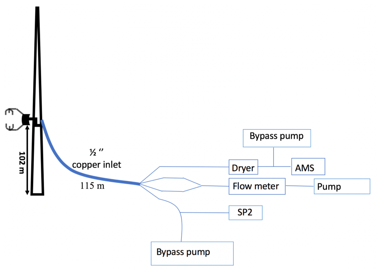
Figure 1Eddy covariance (EC) measurement setup on the IAP tower for BC flux measurements. The aerosol and BC were sampled from an inlet placed at 102 m above ground level. The sonic anemometer 0.75 m from the inlet measured the wind components and virtual temperature.
The raw data recorded by the SP2 are the multi-channel data for individual particles; however only a subset of the particles detected is typically recorded, due to limitations imposed by hard drive space and computer throughput. Since we were operating in a heavily polluted environment, we set the particle recording frequency to 1 in 30 for winter and 1 in 5 for summer. Ideally, every single particle (i.e. 1 in 1) would be analysed to maximise counting statistics and minimise uncertainty in the flux calculation, but limitations in data storage and processing power of the built-in computer prevented this. Count frequencies were based on the instrument performance and ambient concentrations, with concentrations higher in winter.
During acquisition, the instrument handles data in 200 ms buffers, and each recorded particle is timestamped according to the buffer, so when the data are processed, it produces number and mass concentrations with a 5 Hz time resolution. If during acquisition a buffer is not fully processed before the next one has finished collection (which can occur at high concentrations), then a data buffer is discarded, which is manifested as a 200 ms gap in the data. Overall data losses were 7.5 % in winter and 4.2 % in summer. The higher losses in winter were because of the higher concentrations and the fact the SP2-B used an older and lower specification logging computer compared to the newer SP-C used in the summer. This is in spite of the lower data saving frequency. In both seasons, single data gaps were interpolated as they were assumed to be due to dropped buffers. Longer gaps (symptomatic of other instrument problems) were treated as downtime.
2.4 Black carbon flux calculations
The EC method derives the net flux of BC through the horizontal plane at the height of the measurement from the correlation between the fluctuations in the measured vertical wind speed (w) and BC concentrations, which can be related to the flux between the surface and atmosphere (Emerson et al., 2018).
where the net BC flux (FBC) is calculated as the product of the instantaneous fluctuation in vertical wind speed (w′) and in BC concentration (), summed over an averaging period of 30 min. The fluctuations are derived using Reynolds decomposition, e.g. , where the overbar indicates an arithmetic mean. In the atmosphere, such fluctuations are driven by turbulence and have timescales ranging from milliseconds to a few hours. Therefore, the net correlations of these fluctuations are summed over a timescale that is sufficient to capture the majority of fluxes, without non-stationary influences from true changes in emission or meteorology.
We use the widely used open-source software, EddyPro software version 6.2.1 (LI-COR Inc.), to calculate the fluxes as used with CO2 and other greenhouse gas flux measurements. A time lag occurs between wind and BC measurements from the spatial separation of the sonic anemometer and the SP2. Time lags can be determined for each 30 min period, but they can be difficult to quantify when the measurements have a low signal-to-noise ratio and fluxes are associated with higher uncertainty (Langford et al., 2015). Here, time lags are calculated using 24 h periods of 5 Hz data, with application of the covariance maximisation method (Nemitz et al., 2008; Su et al., 2004) giving a time lag for each day. As these are found to be consistent, a mean constant time lag of 13 (winter) and 14 s (summer) is used. For streamline corrections, the double rotation method is used with the three velocity components of the anemometer (Wilczak et al., 2001). Finally, the fluxes were calculated using a linear detrending method for each 30 min of averaging period but only if the averaging period had missing data gaps that accounted for less than 10 % of the data loss. Missing data are caused by either interruption in sampling (e.g. instrument maintenance, calibration) or problems with the logging computer (Sect. 2.2). The random uncertainty in the measurements is calculated following the Finkelstein and Sims (2001) approach.
2.5 Environmental and micrometeorological conditions
The vertical transport of the BC emitted depends on micrometeorology and environmental conditions. The friction velocity (u∗) is a measure of the efficiency of the vertical transport of momentum and thus also of the pollutants (Fig. 2a). During the early hours of the day, in the absence of solar heating, friction velocities are lowest and are more dependent on turbulence generated from wind shear. After sunrise, additional heating (solar, and human activities) can enhance turbulence, making it more buoyant. This increase occurs in both seasons. This effect is stronger in summer as the radiation is stronger and the stored heat is greater (Fig. 2b). Furthermore, it is crucial to confirm that measurements are within the boundary layer, so they can be related to surface emissions. The mixed layer heights (MLHs) are derived from ceilometer (Vaisala CL31, Finland) measurements at the base of the tower using the CABAM algorithm (Kotthaus and Grimmond, 2018). In both seasons the average MLH is greater than the measurement height (Fig. 2c).
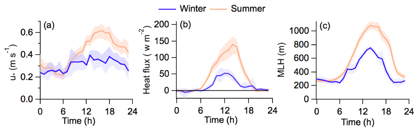
Figure 2Winter (blue) and summer (orange) diurnal pattern of (a) friction velocity (u∗), (b) sensible heat flux and (c) mixed layer height (m). Shaded areas are the interquartile ranges, and the solid line is the mean.
3.1 Stability, stationarity and storage corrections
Rural fluxes are often filtered to remove low friction velocity periods (e.g. u∗ < 0.2 m s−1) when vertical exchange is suppressed, and surface emissions may not reach the measurement height but may instead be advected (e.g Barr et al., 2013). For urban flux measurements, given the large storage and anthropogenic heat fluxes, the urban areas may remain unstable (e.g. Kotthaus and Grimmond, 2012, 2014) or not (Ward et al., 2013), making a single cut-off value of u∗ challenging because, unlike for rural CO2 exchange, times during which fluxes should be independent of u∗ are difficult to predict. This is due to the complex boundary layer behaviour caused by the heterogeneity of the urban canopy, urban heat island effect and release of storage heat to the boundary layer. In this study, we applied a filtering threshold of u∗ ≤ 0.15 m s−1. The data loss from this is higher in winter (21 %) than summer (13 %). Removing these data increases mean BC fluxes; the average mass and number fluxes increased by 10 % during winter and in summer, and the mass and number fluxes increased by 14 % and 13 % respectively. Periods of lower turbulence typically occur at night when the MLH is also lower. In those conditions, without efficient transport of emissions to the measurement height, a build-up in concentration below this level may occur (i.e. positive storage flux). This build-up is typically released later when the boundary layer grows (i.e. negative storage flux). Here, a single-point storage flux correction is calculated as (Rannik and Vesala, 1999)
Here, Fs is the storage flux term, c is the concentration, z is the measurement height and Δt= 30 min. The storage correction was considered when the surface emission was required (e.g. diurnal cycles). For deriving correlations between co-emitted pollutants with the BC flux, storage correction is not applied to any of the metrics as this is not required and could potentially add additional error. The EC method assumes steady-state conditions, which is often not satisfied due to a change in weather patterns and meteorological variables with time of the day. The stationarity test described by Foken and Wichura (1996) is often performed to examine whether a flux is statistically invariant over the averaging period. However, this test is unreliable for small fluxes with large uncertainties (e.g Nemitz et al., 2018); therefore this filter is not applied in this study to avoid flagging of averaging periods as non-stationary irrespective of meteorological conditions.
3.2 Spectral analysis
Spectral analysis is a useful approach for diagnosing the nature of turbulence captured by an EC system (Kaimal et al., 1972). Generally, power spectra of the measured scalar (x) are used to demonstrate an instrument's response to capturing the range of turbulent fluctuations, but the poor BC count statistics (Sect. 2.2) resulted in power spectra that resembled white noise (not shown). Instead, the covariance spectra (vertical wind and scalar, w′T and ) are shown in Fig. 3. To minimise the effect of outliers in the spectra, a median is used (Järvi et al., 2014) with instantaneous fluxes less than 0 ng−2 s−1 (both seasons) and low frictional velocities (less than 0.25 m s−1 in winter and 0.38 m s−1 in summer) removed. BC mass co-spectra show the same co-spectral peak and follow sensible heat co-spectra up to a non-dimensional frequency of 5, at which the effect of noise becomes visible. This covers that majority of the flux contribution which occurs from lower frequencies. The trend in high frequency at the inertial subrange range follows the response as predicted by Kolmogorov theory (Kaimal and Finnigan, 1994) (Fig. 3a, purple), which is evident for sensible heat flux. The high-frequency flux loss due to attenuation was investigated using ogive analysis (Spirig et al., 2005). In Fig. 3b, ogives are calculated by cumulatively summing covariance values of and (starting from lowest frequency) and normalised by total covariance. Similar to spectra analysis, in an ideal condition both and ogives would have the same frequency distribution. In the case of attenuation, a difference could occur, which can be scaled at low frequency, such that the ogive collapses on the ogive. During summer, scaling of 0.91 is required, resulting in a flux loss of 9 %. In the case of winter, as the ogive sits below the ogive, scaling of > 1 required, suggesting the spectrum is damped compared to , which is not physically feasible. Generally, this analysis describes the challenges of emulating flux losses in noisy data, and as the losses are minor, we have not applied this correction.
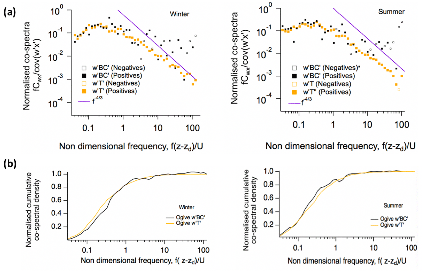
Figure 3(a) Median of BC flux (black) and temperature (sensible heat) (yellow) co-spectrum multiplied by natural frequency (f) and normalised using total covariance against non-dimensional frequency. Data are binned into 44 logarithmically evenly spaced bins, and co-spectra with total BC flux > 0 ng−2 s−1 and carefully selected frictional velocity for more turbulent periods (see Sect. 3.2) were chosen for median averaging. A total of 223 (winter) and 170 (summer) cases are averaged. (b) Normalised cumulative co-spectra of BC flux and sensible heat flux.
4.1 Tower and ground comparison
The physical properties of BC in Beijing during this campaign for both seasons have been discussed by Yu et al. (2020) and Liu et al. (2019) based on the concurrent ground-level SP2 observations. The mass ratio of internally mixed non-BC material (the “coating”) to BC was quantified by Yu et al. (2020), which varied from 2 to 12 in the winter season and 2 to 3 in the summer season. The higher variability during the winter was related to a combination of frequent occurrences of heavy haze episodes and the presence of additional sources compared to the summer seasons. Liu et al. (2019) performed source apportionment analysis for the same ambient BC measurements and identified four different BC modes, which were then compared with AMS and SP-AMS measurement to relate each mode to their potential pollutant source. These four modes were identified using the Esca method described in Sect. 2.2 and include thickly coated (coating diameter, ct > 200 nm); small, thinly coated (ct < 50 nm and Dc < 180 nm); moderately coated (50 nm > ct < 200 nm); and large, thinly coated (ct < 50 nm and Dc > 180 nm) particles. Their study also suggested that thinly coated particles had a strong association with traffic-related activities. Moderately coated and large, thinly coated particles were related to a combination of solid fuel sources (biomass and coal), and thickly coated particles were most associated with atmospheric ageing. Since our study aimed to measure BC fluxes for particles characterised according to their sources, a similar analysis was performed for the tower-level measurements as well as ground level, to understand the suitability of tower-level measurements for drawing similar source characterisations. Firstly, here we compare the concentrations of BC at both levels. Figure 4a shows the overlap periods of both measurements, and Fig. 4b shows correlation between the two sampling heights with an R2 = 0.94 and 0.70 for winter and summer, respectively. During winter, we observe a systematic difference between tower and ground measurement after the data gap on 25 November, corresponding to instrument maintenance for the ground-level SP2, which may have altered its performance. The difference was quantified by separating two periods and recalculating slopes comparing the tower and ground measurements as shown in Fig. 4c. From this, we can infer that the ground measurements increased by 24 %. Furthermore, for tower measurements, there were also particle line losses, and the upper limit of line losses would be 34 %. This is based on the highest difference observed in winter seasons between two levels, although the true losses are likely to be lower than this, as we expect concentrations at ground level to be higher. Secondly, we characterised the mixing state of the particles for the tower level using the same scattering enhancement method as Liu et al. (2019), which is shown in Fig. 5. The two chosen scenarios include polluted and clear periods to capture a variety of BC sources. Our analysis shows similar characteristics of the physical properties of BC to those observed from the ground measurements. Instead of four distinctive modes, we see some overlaps between those modes. This could be due to the use of an older generation of SP2 model but also possibly because during the measurements the flux instrument operated at relatively low laser power, either of which could have reduced the signal-to-noise ratio of the scattering channels. Therefore, we have grouped our measurements into two groups: heavily coated particles(Esca > 3) and lightly coated particles (Esca < 3). The implication of heavily coated particles in this study refers to the combination of thickly coated and moderately coated particles, while lightly coated particles in this study refer to the combination of small, thinly coated and large, thinly coated particles, defined and grouped by Liu et al. (2019).
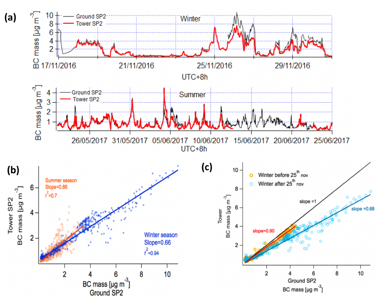
Figure 4(a) Comparisons of BC concentrations at 5 m (black) and 102 m (red) in winter and summer. (b) Correlation of BC concentrations measured at the two different levels for winter (blue) and summer (orange). (c) Correlation of BC mass concentrations before and after 25 November.
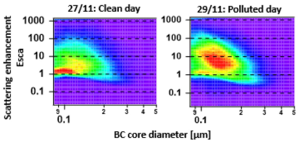
Figure 5BC particles physical properties on a clean and a polluted day. Scattering enhancement measured using the method discussed by Liu et al. (2019). When the particle number density (colour) is > 70 % of the maxima in each panel, then the colour is set to red.
4.2 Black carbon fluxes
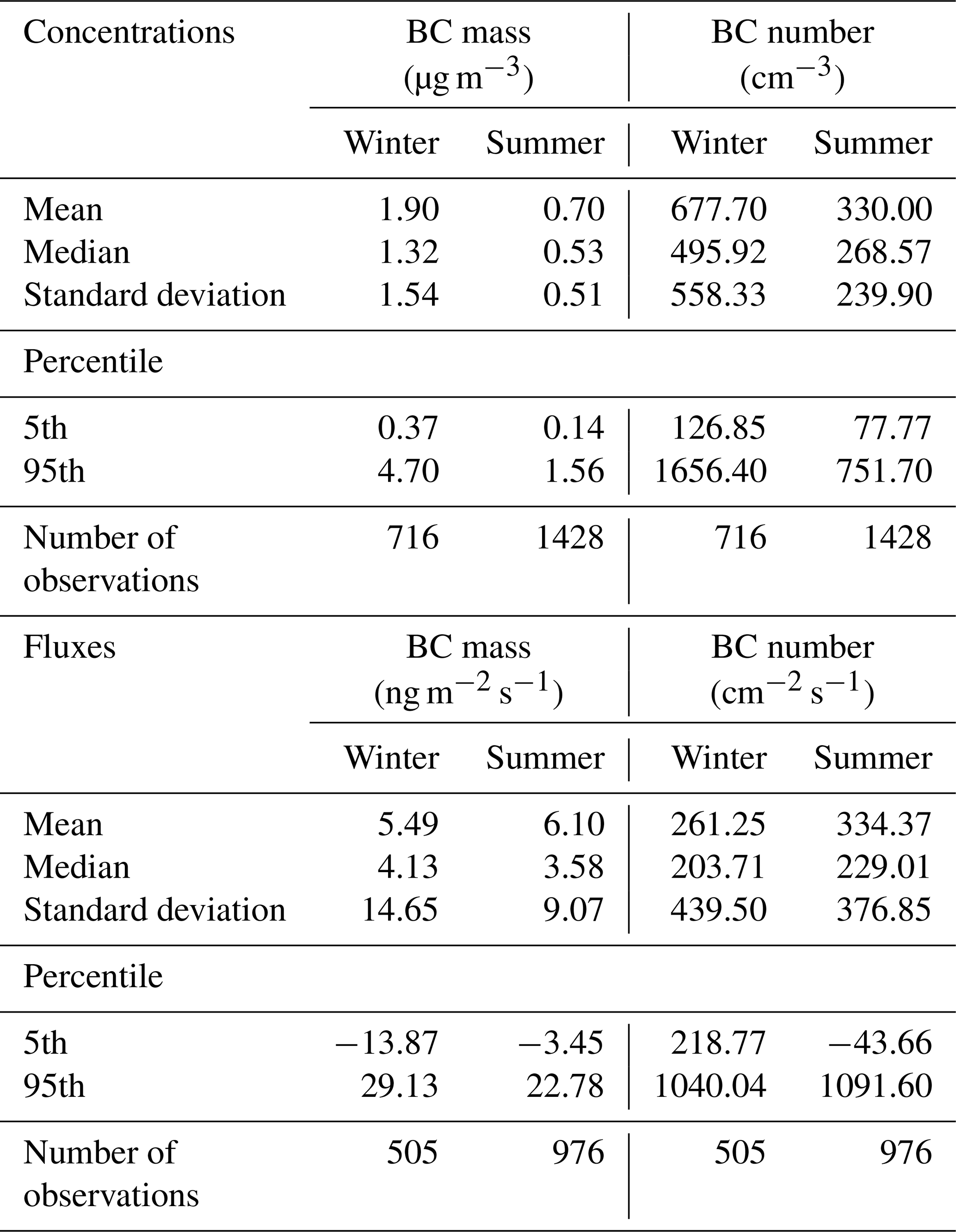
Figure 6 shows 30 min fluxes of BC mass and number for both the winter and summer periods. The signal-to-noise ratio of the mass fluxes in particular is low, and fluxes vary throughout the measuring period, due to the variability in emissions in the flux footprint, e.g. in response to activities and time of the day. However, mainly positive fluxes were observed, confirming a net emission of BC from the city. During the winter period, measurement coverage was lower (total number of 30 min averaging interval = 505) compared with the summer (total number of 30 min averaging interval = 976). Mean averaged mass fluxes (with associated standard error) of 5.49 ± 0.49 and 6.10 ± 0.18 ng m−2 s−1 were measured during the winter and summer, respectively. For the BC number flux, averages of 261.25 ± 10.57 and 334.37 ± 0.37 cm−2 s−1 were measured. In order to remove any time-of-day biases associated with missing or filtered data, gaps in the data could be replaced with the corresponding average diurnal value. This delivers modified BC mass fluxes of 5.22 and 6.06 ng m−2 s−1 for winter and summer respectively and BC number fluxes of 252.41 and 334.40 cm−2 s−1. The uncertainty of the measurements is shown with black error bars in Fig. 6. The calculation of such uncertainty was performed by calculating the random error (RE) of each averaging period following the method discussed by Finkelstein and Sims (2001). The mass flux is associated with a larger uncertainty than the number flux as the mass flux suffers from poor counting statistics since few particles with large BC mass make a large contribution to the total flux. The winter measurements are associated with higher uncertainty due to the lower atmospheric turbulence, and the higher incidence of extreme values is consistent with this noise. As such, no individual 30 min deposition events can be discerned with any statistical certainty. Therefore, we did not unpick such events/criteria and instead discussed averaged flux results in this study. It is important to note that aerosol flux measurements tend to have higher RE than gas flux measurements. While the point-by-point data are of low precision, averaging of the fluxes according to either diurnal cycle or wind sector can deliver more meaningful statistics, and this is discussed in the following section. Additionally, the summary of BC concentrations and fluxes is also provided in Table 1.
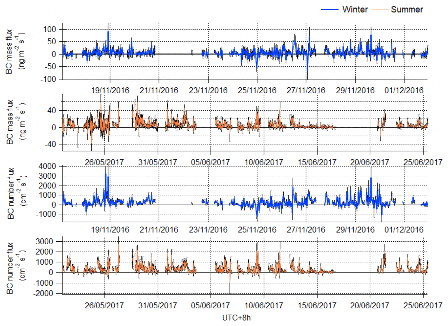
Figure 6Time series of 30 min averaged fluxes during winter (blue) and summer (orange) for mass and number fluxes, with random errors caused by associated uncertainties of the EC measurement system of this study (black bars).
Table 1Concentration and flux statistics of BC measurements at the IAP tower. The 5 Hz concentration measurements were resampled 30 min before performing statistical calculations.
4.3 Local black carbon characterisation
The flux footprint represents the local area that contributes to the measured flux. The shape and size of the flux footprint is related to the sampling height, wind speed and direction, atmospheric stability, surface roughness, turbulence and the boundary layer height. Figure 7 depicts the extent of the average flux footprint for the winter and summer measurement periods, respectively. These footprints were generated using the method presented by Squires et al. (2020), using the footprint model and theory discussed by Kljun et al. (2004) and Metzger et al. (2012). However, the total numbers of individual footprints used to generate average campaign footprints are slightly different to those presented by Squires et al. (2020), owing to slight differences in the respective instrument uptimes. The footprints were superimposed onto a map of Beijing at a grid resolution of 10 × 10 m. The initial comparison between the seasons shows that the averaged sizes of the footprints were similar. Here, the counter circles represent 30 %, 60 % and 90 % cumulative contribution to the measured averaged fluxes from those regions. During both seasons, the majority (up to 90 %) of contributions reached about 2 km from the IAP tower. However, within that range, maxima of the contribution occurred at a distance of 0.26 km. The major difference between the two seasons was the change in the dominant wind directions. During winter, the wind direction was predominantly from the north-west, and hence measurements are likely to have captured emissions from Beitucheng West Road in the NW direction. During summer, winds were predominantly from the north-east direction, capturing emissions from the major Jingzang Expressway. Since this analysis indicates the presence of traffic-related emissions, we have shown diurnal trends as well as their spatial intensity according to their wind speed and direction in the following section.
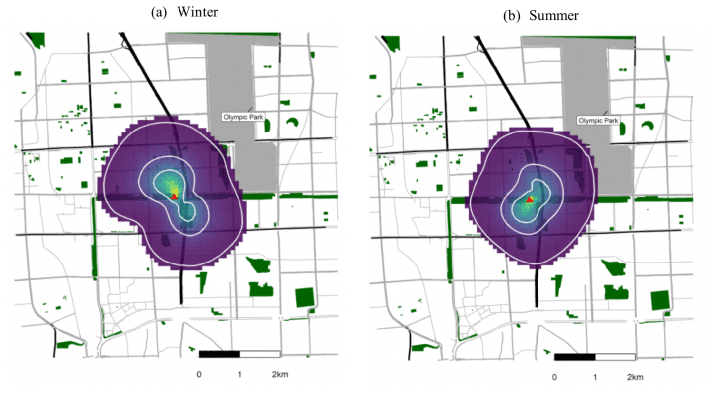
Figure 7Total average mass flux footprints for winter and summer seasons. The red spot on each plot is the location of the IAP tower, and surrounding colours represent the magnitude of the intensity of the measured emission. The resolution of footprint is 100 m2, the outermost white line represents the 90 % cumulative spatial contribution of the total flux and the middle and the innermost lines represent 60 % and 30 % contribution. Map was built using data from © OpenStreetMap contributors 2020. Distributed under a Creative Commons BY-SA License. The ring roads are shown in black, and other roads are shown in grey. Parks/green spaces are shown in green.
4.4 Diurnal and wind sector trends
Figure 8 shows the diurnal cycles for mass and number fluxes, for winter (blue) and summer (orange), and error bars represent the associated averaged random errors (e.g. ). These were calculated using the ensemble average of RE for each diurnal hour as
where N is the number of 30 min averaging periods that entered into generating the average value for each hour of the day.
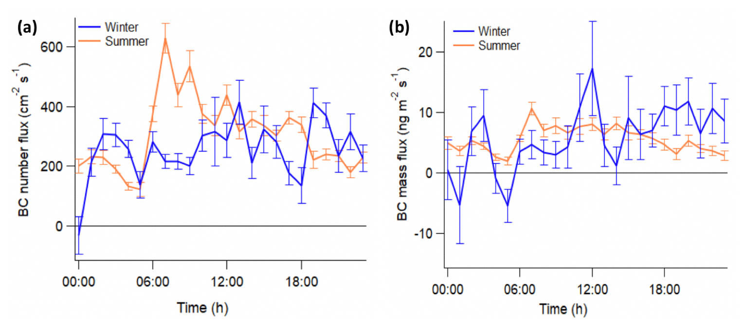
Figure 8Diurnal cycles for (a) number and (b) mass flux in summer and winter with error bars (standard errors, from the calculated precision). For this analysis, storage-corrected fluxes are used to help understand ground-based emissions.
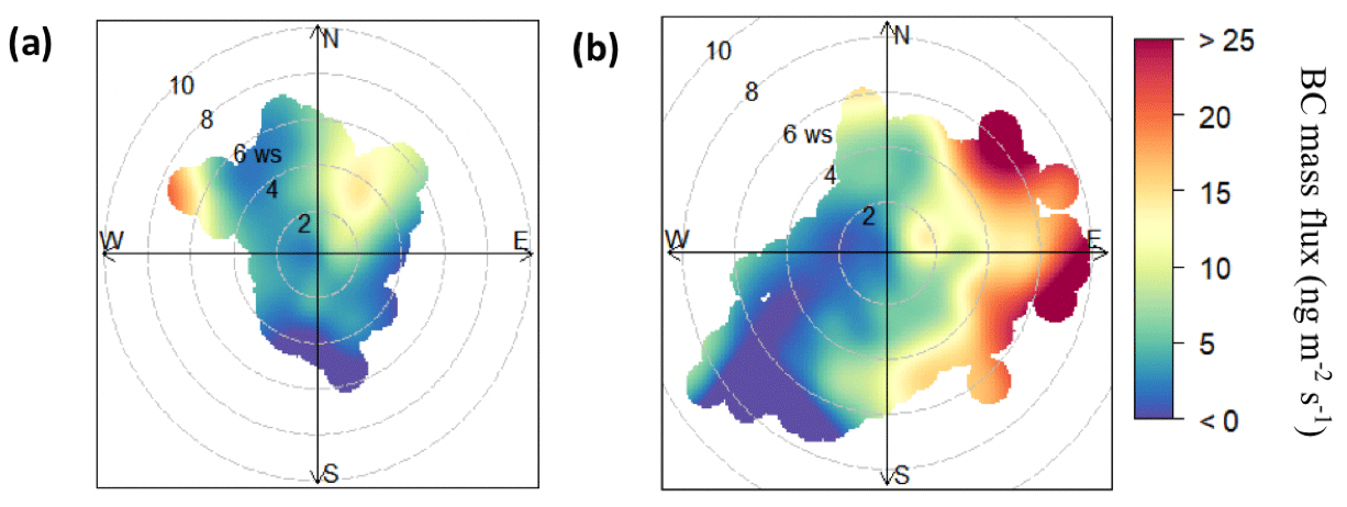
Figure 9BC mass flux distribution by wind direction and wind speed for the (a) winter and (b) summer analysis done using OpenAir software (Carslaw and Ropkins, 2012).
During winter, for both mass and number flux, there were no clear diurnal cycles. In summer there was a clear peak at 07:00, which could be related to traffic-related activities, but there was no distinctive peak for the evening rush hour. However, the average flux values between the two seasons were similar, which is consistent with the source being the same in both seasons. For both seasons, BC diurnals showed similar patterns to those of CO and NOx fluxes (Squires et al., 2020), suggesting that traffic emissions are the dominant source of BC in this region of Beijing. Therefore, we additionally averaged BC fluxes according to wind sector and generated polar plots using OpenAir (Carslaw and Ropkins, 2012) for mass fluxes, as shown in Fig. 9. This analysis clearly shows that fluxes were largest in the NE direction during both seasons. This is crucial as, during the winter, the NE is not a prominent wind direction as we discussed in the footprint analysis section. The analysis would suggest that the strongest sources lie in the NE and E directions, which is consistent with the presence of a major traffic junction. During the summer, the indications that the major source is traffic-related (such as the diurnal profile) are generally clearer, due to better coverage and signal-to-noise ratio, turbulence and favourable wind direction. The quantification of traffic emissions is discussed in the following section.
4.5 Flux for characterised black carbon particles
In Sect. 4.1 the source apportionment of BC particles, according to their coating content, was discussed using the threshold value of Esca= 3; particles above this threshold are defined as heavily coated, and the rest of the particles are lightly coated. The lightly coated mode contains BC particles with a strong association with traffic-related sources; however within this mode, BC particles with Dc > 180 could possibly be associated with solid fuel burning, according to BC source apportionment, discussed by Liu et al. (2019). Therefore, in this analysis, we firstly separated BC mass and BC number concentrations using a threshold value of Esca= 3 and defined this characteristic as coating classification. Additionally, we used a threshold of Dc= 180 nm to perform the size classification.
The average mass and number concentration of lightly coated and heavily coated particles are shown in Table 2. Almost a quarter of the BC mass concentrations (and slightly less than a quarter if we consider number concentrations) measured at IAP were from the heavily coated mode, and the rest of the particles were from the lightly coated mode. In order to quantify what proportion of these particles was emitted locally, fluxes of each individual categories were also calculated, and their average values are also summarised in Table 2. We can see that the contribution of BC particles emitted from heavily coated was smaller than 8 % for both BC mass and number fluxes, with the lightly coated mode accounting for 92.3 % of both fluxes.
Table 2Winter season percentage values of concentrations and fluxes for coating classification and size classification. For coating classification, the total particles were separated according to coating contents using the threshold of Esca= 3 for both BC mass and number. For size classification, the total particles were separated at Dc= 180 nm, for BC mass and number. During summer, such an analysis was not performed due to limitations of the instrument at the time of the experiment.
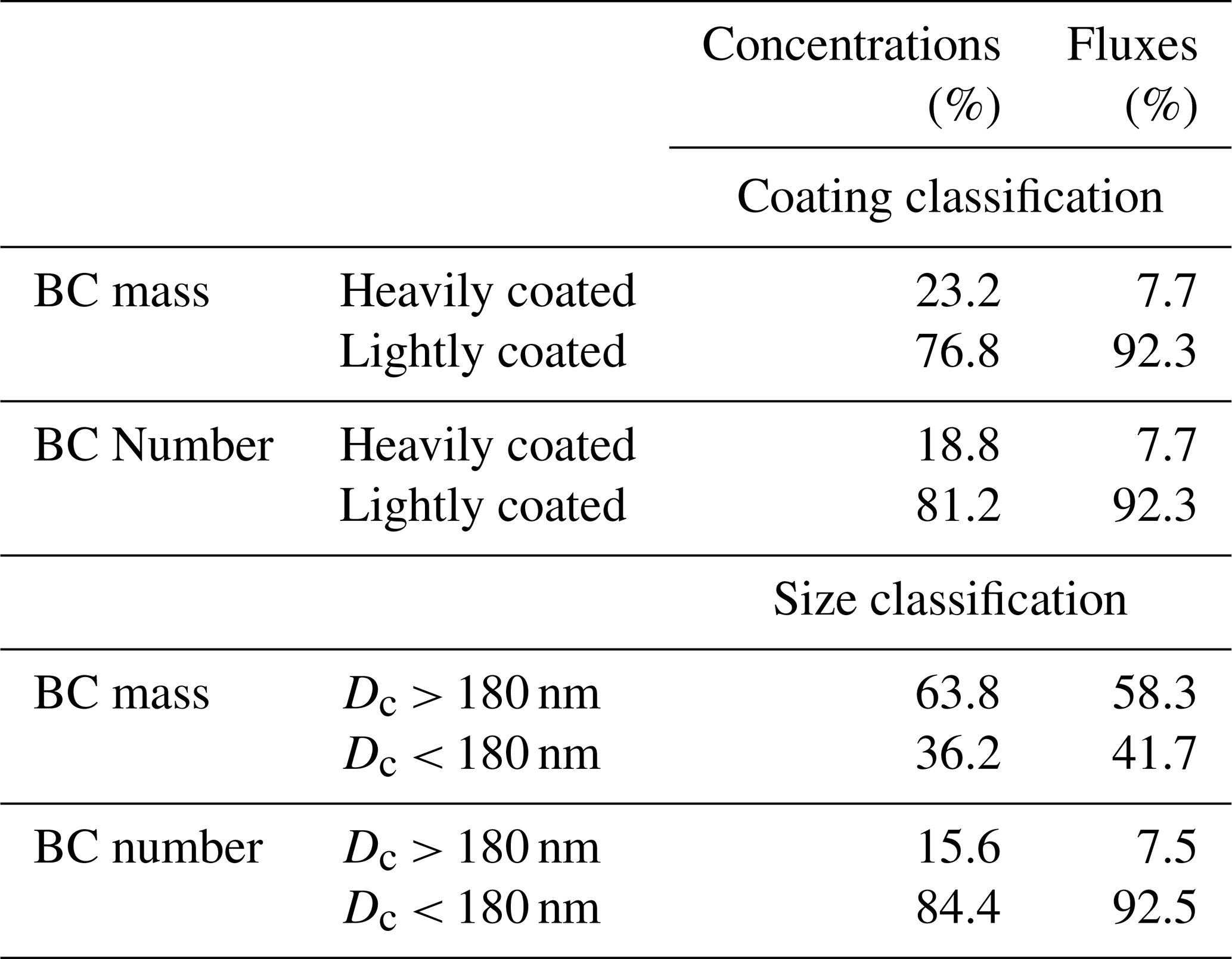
Regarding size classification, it is important to note that there were fewer particles above this range; yet they contributed significantly to the concentration in mass space. Therefore, this analysis suffers from poor counting statistics, and we cannot reliably quantify emissions for particles with Dc > 180 nm. However, the general trend for both BC mass and BC number quantity in Table 2 for the size classification shows that the average fraction of particles Dc > 180 nm is higher for concentrations compared to their fraction of the total flux measurements, indicating that the majority of these particles are from outside of the flux footprint. As the majority of emissions within the flux footprints are in the form of lightly coated particles, this is consistent with this particle type being associated with traffic-related activities.
5.1 Comparison with NOx and CO emissions
With the assumption that CO and NOx are co-emitted with BC by combustion sources, we have investigated the correlations of their measured fluxes with BC using orthogonal distance regression. These are shown in Fig. 10a and b, for CO and NOx, respectively, and the gradients in each plot correspond to the emission flux ratios. The comparison with CO fluxes shows BC ∕ CO mass ratios of 0.0007 and 0.0011 for winter and summer, respectively. During the summer, this ratio is 37 % larger than in winter. Our study has shown similar emissions of total averaged BC in the two seasons; however, this is not the case for CO. During winter, cold-start conditions may explain the increase in CO emission, which is further discussed by Squires et al. (2020). The comparison with NOx fluxes shows BC ∕ NOx ratios are the same between seasons, 0.0058 and 0.0052 for winter and summer, respectively. The relationship in winter shows more scatter due to a poor signal-to-noise ratio. Nevertheless, the consistency of the NOx slopes is highly encouraging as the identical relationship is not only consistent with the emissions being from a singular dominant source, i.e. vehicles, but also provides confidence in the measurements, given that a physically different instrument was used in the two seasons.
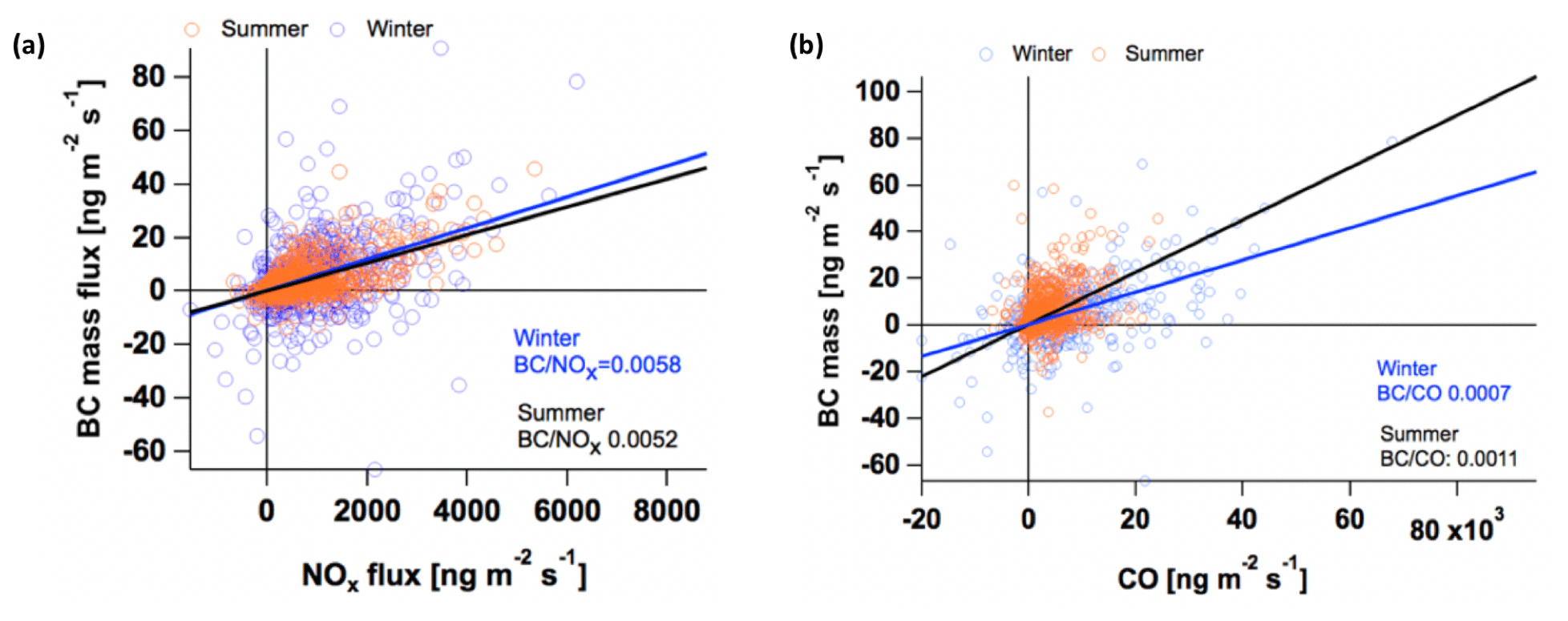
Figure 10BC mass flux with (a) NOx flux (Squires et al., 2020) and (b) CO flux (Squires et al., 2020) for winter and summer with calculated BC ∕ NOx and BC ∕ CO ratios and NOx and CO fluxes converted to the same units as our measurements.
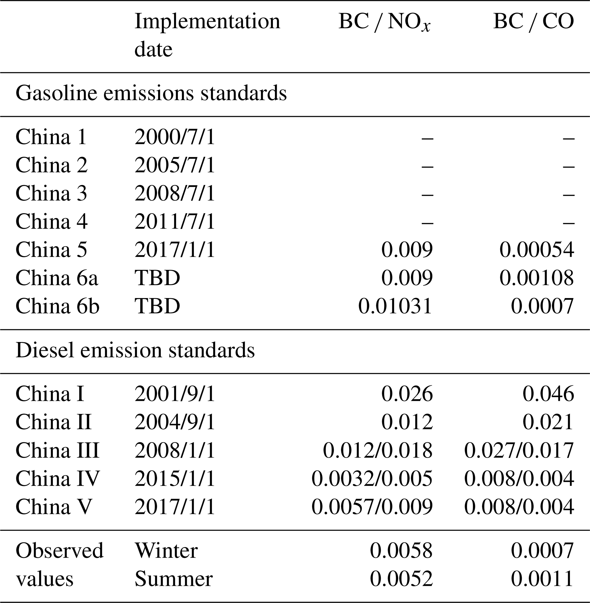
Following a similar vehicular European regulation system for emission controls, China has started to adopt emission regulation targets. The limits imposed cover the major pollutants CO, NOx, non-methane hydrocarbon (NMHC), HC + NOx and PM (which refers to PM2.5) for both light-duty gasoline vehicles (LDGVs) and heavy-duty diesel engines (HDDEs), as summarised by Wu et al. (2017). However, to the best of our knowledge, reliable values of BC fraction within PM2.5 are not available in literature for China's regulation standards. Therefore, we used the average BC ∕ PM2.5 ratios for gasoline engines from the European guidelines of emissions controls as stated in Table 3.2.1 of Ntziachristos and Samaras (2017), which are 0.12 and 0.57 for gasoline and diesel engines, respectively. Using these ratios, we have estimated BC ∕ NOx and BC ∕ CO ratios implied with each of China emission's standards for both LDGVs and HDDEs, as shown in Table 3. It is important to note that PM2.5 controls for LDGVs were only introduced recently from 1 January 2017 as part of China 5 controls. If we compare our measured emission ratios as shown in Fig. 10 with the values in Table 3, we find that the measured values are in a similar range as the ratio of China 5 limit levels for gasoline emissions, noting that diesel vehicles are banned from central Beijing during the daytime and are therefore not expected to contribute. Making the implicit assumption that the legal limits are a fair reflection of actual emissions, this is in a good agreement.
Table 3Estimated ratios of BC ∕ NOx and BC ∕ CO for gasoline engines and diesel engines. An overview of on-road vehicular emissions and their control in China by Wu et al. (2017) summarised NOx, CO and PM2.5 emission regulation targets in China. The BC ∕ PM2.5 fractions for gasoline were taken from European guideline of emissions controls, as such fractions are not available for China. Since PM2.5 controls for LDGVs were only introduced recently within China 5 controls, our estimates could not be performed according to previous standards. Observed values correspond to ratios shown in Fig. 10. Dates are given in yyyy/mm/d. TBD denotes standards that are “to be decided”.
5.2 Emission inventory
Here we compare our measurements with the Multi-resolution Emission Inventory for China (MEIC; available at http://www.meicmodel.org/, last access: 2 November 2019), developed at Tsinghua University (e.g Zhang et al., 2015). The inventory uses spatial proxies (e.g. population and energy consumption statistics) to downscale emissions from a national and provincial scale to finer resolution (Biggart et al., 2020; Qi et al., 2017). In this study, BC emissions for the year 2013 at a resolution of 3 × 3 km were used, which was the most recent version available at the time of this study. The inventory emission values were extracted for the area covered by the averaged flux footprint (see Sect. 4.3) following the same approach as Squires et al. (2020).
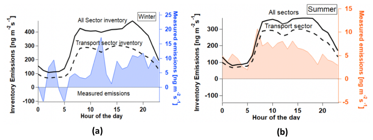
Figure 11Comparison between measured emissions and the MEIC 2013 emission inventory for (a) winter and (b) summer for the flux footprint area (Sect. 4.3). Diurnal variation from the MEIC estimates is used for the diurnal cycles for emissions of all sectors (sum of emissions from transport, industry, residential and power) and the transport sector in isolation.
Figure 11 shows a comparison of the diurnal cycles between measured fluxes and the MEIC 2013 emission inventory for (a) winter and (b) summer, where the diurnal cycles for each sector (transport, industry, agriculture, residential and power) were generated from the MEIC 2013 estimates.
The inventory has a broadly similar temporal pattern to the observed fluxes but overestimates the total BC emissions from the flux footprint by a factor of 59 and 47 during the winter and summer periods, respectively. Since the transport sector contributes 63 % and 80 % of the overall BC emissions in the MEIC inventory, the average emissions of the transport sector in isolation were also compared with the measured flux. This reduced the discrepancy to within a factor of 38 for both winter and summer periods.
The reduction in emissions in Beijing from 2013 to 2017 has been analysed by Cheng et al. (2019) using the MEIC model in combination with a local bottom-up emission inventory. This study concludes that the reduction in PM2.5 emissions from the transport sector is negligible, as since 2013 there has been an increase in stringent traffic management and fuel control policies, but vehicle densities have increased, keeping emissions from the transport sector steady. This is also discussed on a national level for BC emissions from the transport sector by Zheng et al. (2018), and it was concluded that emissions from the transport sectors remained steady between 2010 and 2017. Therefore, such a large discrepancy is unlikely to be due to changes in actual emissions between 2013 and 2017. We also compared BC ∕ CO and BC ∕ NOx ratios for the transport emission data in MEIC, which were 0.0066, 0.0423 and 0.0072, 0.0425 for the winter and summer seasons, respectively. Compared to the observed ratios, these are factors of 9.4 and 6.5 too high for the ratios with CO in winter and summer respectively and 7.3 and 8.1 for the ratios with NOx. This implies that the BC emissions from traffic are overestimated in MEIC, although it should be noted that the emissions of NOx and CO from the inventory are also high compared with measured fluxes, as reported by Squires et al. (2020). The overestimation of emissions in this region may reflect the limited suitability of the proxies used in downscaling the emissions from a regional, provincial resolution to the 3 km scale used here, as noted by Zheng et al. (2017). However, the overestimation of the ratios highlights that it is likely that BC emissions are overestimated in MEIC, at least for the region considered here. The diurnal patterns of emissions, in contrast, are in relatively good agreement.
Local emissions of BC fluxes were measured using the eddy covariance method in Beijing as part of the APHH project during the winter of 2016 and summer of 2017 from the IAP tower, the first application of this approach to an urban environment. During both seasons, average BC mass flux and number fluxes remained stable. In the case of BC mass fluxes, average values of 5.5 ± 0.49 and 6.1 ± 0.18 ng m−2 s−1 were measured during the winter and summer seasons, respectively. In the case of BC number fluxes, average values of 261.3 ± 10.57 and 334.4 ± 0.37 cm−2 s−1 were measured for the winter and summer seasons, respectively. The similarity in the magnitude of emissions between seasons suggests that there was no major additional source in winter associated with heating, consistent with the use of district heating in central Beijing. Flux footprints (up to 2 km from the IAP tower in both seasons) and wind sector-based analysis showed emission sources are strongest to the NE and E of the IAP tower, where a major road is situated, confirming the presence of traffic emissions. The contribution of traffic emission was quantified by classifying total BC particles according to coating thickness during the winter season, following the previous observation that traffic emits smaller, more lightly coated particles. The analysis indicated traffic emissions were approximately 92 % of the total measured flux for both BC mass and BC number fluxes, and the rest was possibly associated with solid fuel burning. In terms of the overall concentrations, the heavily coated particles represented 23 % and 19 % of the BC mass and number concentrations respectively. The higher presence of the heavily coated particles in concentration measurements but not local fluxes suggests advection of a source outside the footprint and is indicative of regional pollution. The measurements were also compared with NOx and CO fluxes and the corresponding emission ratios BC ∕ CO and BC ∕ NOx were inferred. The BC ∕ NOx ratio was found to be consistent between seasons, and both ratios were in general agreement with ratios implied by the China emission standards. Finally, the measured emissions were compared with the MEIC 2013 inventory. The magnitude of the transport sector emissions in the inventory alone was significantly larger (by over an order of magnitude) than our measurements. Such a discrepancy cannot solely be explained by changes in emissions since 2013, indicating that there are other inaccuracies, likely in the proxies used to downscale the emissions to an urban landscape as noted by Zheng et al. (2017). The shape of the diurnal variation in the inventory was in better agreement; however, the BC ∕ CO and BC ∕ NOx ratios from the MEIC inventory were substantially larger than the measured ratios, which could indicate that an inaccuracy in the assumed BC emission profile is at least partially responsible for the disagreement. This indicates that BC emissions in the inventory are overestimated, at least in the urban area of Beijing.
Processed data are available in the APHH-Beijing project database in the Centre for Environmental Data Analysis Archive (http://data.ceda.ac.uk/badc/aphh/data/beijing/, Fleming et al., 2017). Raw data are available on request.
RJ made the measurements, performed data analysis and wrote the paper with support from JA, HC and DL. DL helped with developing the toolkit for the preprocessing of SP2 flux data and provided guidance with source apportionment of work. NM installed and maintained the tower EC measurement setup. EN and BL helped RJ with flux calculations and the use of the EddyPro software. FS and JL provided flux footprint calculations, with corresponding emission inventory data. YW, XP and PF allowed the use of their SP2 instrument during the summer season. SK and SG provided the mixed layer height data. QZ and RW provided MEIC inventory data, and OW helped with the interpretation of the inventory values. MF provided technical support for maintenance of the SP2 instruments. HC and JA are PhD supervisors of RJ. All the authors read and improved the paper.
The authors declare that they have no conflict of interest.
This article is part of the special issue “In-depth study of air pollution sources and processes within Beijing and its surrounding region (APHH-Beijing) (ACP/AMT inter-journal SI)”. It is not associated with a conference.
Rutambhara Joshi's PhD was supported by the National Centre of Atmospheric Science (NCAS). The field measurements were supported by the Newton Fund, administered by the UK Natural Environment Research Council (NERC) through the AIR-POLL and AIRPRO projects of the Air Pollution and Human Health in a Chinese Megacity (APHH-Beijing) programme.
This research has been supported by the Natural Environment Research Council (grant nos. NE/N006992/1, NE/N006976/1, NE/N006917/1, NE/N007123/1 and NE/N00700X/1).
This paper was edited by Markus Petters and reviewed by two anonymous referees.
Barr, A. G., Richardson, A. D., Hollinger, D. Y., Papale, D., Arain, M. A., Black, T. A., Bohrer, G., Dragoni, D., Fischer, M. L., Gu, L., Law, B. E., Margolis, H. A., Mccaughey, J. H., Munger, J. W., Oechel, W., and Schaeffer, K.: Use of change-point detection for friction-velocity threshold evaluation in eddy-covariance studies, Agr. Forest Meteorol., 171–172, 31–45, https://doi.org/10.1016/j.agrformet.2012.11.023, 2013.
Barrington-Leigh, C., Baumgartner, J., Carter, E., Robinson, B. E., Tao, S., and Zhang, Y.: An evaluation of air quality, home heating and well-being under Beijing's programme to eliminate household coal use, 4, 416–423, https://doi.org/10.1038/s41560-019-0386-2, 2019.
Biggart, M., Stocker, J., Doherty, R. M., Wild, O., Hollaway, M., Carruthers, D., Li, J., Zhang, Q., Wu, R., Kotthaus, S., Grimmond, S., Squires, F. A., Lee, J., and Shi, Z.: Street-scale air quality modelling for Beijing during a winter 2016 measurement campaign, Atmos. Chem. Phys., 20, 2755–2780, https://doi.org/10.5194/acp-20-2755-2020, 2020.
Bond, T. C. and Bergstrom, R. W.: Light Absorption by Carbonaceous Particles: An Investigative Review, Aerosol Sci. Tech., 40, 27–67, https://doi.org/10.1080/02786820500421521, 2006.
Bond, T. C., Streets, D. G., Yarber, K. F., Nelson, S. M., Woo, J.-H., and Klimont, Z.: A technology-based global inventory of black and organic carbon emissions from combustion, J. Geophys. Res.-Atmos., 109, D14203, https://doi.org/10.1029/2003JD003697, 2004.
Bond, T. C., Doherty, S. J., Fahey, D. W., Forster, P. M., Berntsen, T., Deangelo, B. J., Flanner, M. G., Ghan, S., K??rcher, B., Koch, D., Kinne, S., Kondo, Y., Quinn, P. K., Sarofim, M. C., Schultz, M. G., Schulz, M., Venkataraman, C., Zhang, H., Zhang, S., Bellouin, N., Guttikunda, S. K., Hopke, P. K., Jacobson, M. Z., Kaiser, J. W., Klimont, Z., Lohmann, U., Schwarz, J. P., Shindell, D., Storelvmo, T., Warren, S. G., and Zender, C. S.: Bounding the role of black carbon in the climate system: A scientific assessment, J. Geophys. Res.-Atmos., 118, 5380–5552, https://doi.org/10.1002/jgrd.50171, 2013.
Cao, G., Zhang, X., and Zheng, F.: Inventory of black carbon and organic carbon emissions from China, Atmos. Environ., 40, 6516–6527, https://doi.org/10.1016/j.atmosenv.2006.05.070, 2006.
Carslaw, D. C. and Ropkins, K.: Openair – An r package for air quality data analysis, Environ. Model. Softw., 27–28, 52–61, https://doi.org/10.1016/j.envsoft.2011.09.008, 2012.
Cheng, J., Su, J., Cui, T., Li, X., Dong, X., Sun, F., Yang, Y., Tong, D., Zheng, Y., Li, Y., Li, J., Zhang, Q., and He, K.: Dominant role of emission reduction in PM2.5 air quality improvement in Beijing during 2013–2017: a model-based decomposition analysis, Atmos. Chem. Phys., 19, 6125–6146, https://doi.org/10.5194/acp-19-6125-2019, 2019.
Emerson, E. W., Katich, J. M., Schwarz, J. P., McMeeking, G. R., and Farmer, D. K.: Direct Measurements of Dry and Wet Deposition of Black Carbon Over a Grassland, J. Geophys. Res.-Atmos., 123, 12,277-12,290, https://doi.org/10.1029/2018JD028954, 2018.
Finkelstein, P. L. and Sims, P. F.: Sampling error in eddy correlation flux measurements, J. Geophys. Res.-Atmos., 106, 3503–3509, 2001.
Fleming, Z. L., Lee, J. D., Liu, D., Acton, J., Huang, Z., Wang, X., Hewitt, N., Crilley, L., Kramer, L., Slater, E., Whalley, L., Ye, C., and Ingham, T.: APHH: Atmospheric measurements and model results for the Atmospheric Pollution & Human Health in a Chinese Megacity, Centre for Environmental Data Analysis Archive, available at: http://data.ceda.ac.uk/badc/aphh/data/beijing/ (last access: 4 January 2021), 2017.
Foken, T. and Wichura, B.: Tools for quality assessment of surface-based flux measurements, Agr. Forest Meteorol., 78, 83–105, https://doi.org/10.1016/0168-1923(95)02248-1, 1996.
Gao, R. S., Schwarz, J. P., Kelly, K. K., Fahey, D. W., Watts, L. A., Thompson, T. L., Spackman, J. R., Slowik, J. G., Cross, E. S., Han, J. H., Davidovits, P., Onasch, T. B., and Worsnop, D. R: A novel method for estimating light-scattering properties of soot aerosols using a modified single-particle soot photometer, Aerosol Sci. Tech., 41, 125–135, 2007.
Harrison, R. M., Deacon, A. R., Jones, M. R., and Appleby, R. S.: Sources and processes affection concentrations of PM10 and PM2.5 particulate matter in Birmingham (U.K.), Atmos. Environ., 31, 4103–4117, https://doi.org/10.1016/S1352-2310(97)00296-3, 1997.
Hodnebrog, Ø., Myhre, G., and Samset, B. H.: How shorter black carbon lifetime alters its climate effect, Nat. Commun., 5, 1–7, 2014.
Järvi, L., Nordbo, A., Rannik, Ü., Haapanala, S., Mammarella, I., Pihlatie, M., Vesala, T., and Riikonen, A.: Urban nitrous-oxide fluxes measured using the eddy-covariance technique in Helsinki, Finland, Boreal Environ. Res., 19, 108–121, 2014.
Jassen, N. A. H., Gerlofs-Nijland, M. E., Lanki, T., Salonen, R. O., Cassee, F., Hoek, G., Fischer, P., Brunekreef, B., and Krzyzonowsk, M.: Health Effects of Black Carbon, World Health Organization, Regional Office for Europe, available at: http://www.euro.who.int/__data/assets/pdf_file/0004/162535/e96541.pdf (last access: 5 January 2021), 2012.
Kaimal, J. C. and Finnigan, J. J.: Atmospheric boundary layer flows: their structure and measurement, Oxford university press, New York, USA, 1994.
Kaimal, J. C., Wyngaard, J., Izumi, Y., and Cote, O.: Spectral characteristics of surface-layer turbulence, Q. J. Roy. Meteor. Soc., 98, 563–589, https://doi.org/10.1256/smsqj.41706, 1972.
Kljun, N., Calanca, P., Rotach, M. W., and Schmid, H. P.: A simple parameterisation for flux footprint predictions, Bound.-Lay. Meteorol., 112, 503–523, https://doi.org/10.1023/B:BOUN.0000030653.71031.96, 2004.
Kotthaus, S. and Grimmond, C. S. B.: Identification of Micro-scale Anthropogenic CO2, heat and moisture sources – Processing eddy covariance fluxes for a dense urban environment, Atmos. Environ., 57, 301–316, https://doi.org/10.1016/j.atmosenv.2012.04.024, 2012.
Kotthaus, S. and Grimmond, C. S. B.: Energy exchange in a dense urban environment – Part I: Temporal variability of long-term observations in central London, Urban Clim., 10, 261–280, https://doi.org/10.1016/j.uclim.2013.10.002, 2014.
Kotthaus, S. and Grimmond, C. S. B.: Atmospheric boundary-layer characteristics from ceilometer measurements. Part 1: A new method to track mixed layer height and classify clouds, Q. J. Roy. Meteor. Soc., 144, 1525–1538, https://doi.org/10.1002/qj.3299, 2018.
Laborde, M., Mertes, P., Zieger, P., Dommen, J., Baltensperger, U., and Gysel, M.: Sensitivity of the Single Particle Soot Photometer to different black carbon types, Atmos. Meas. Tech., 5, 1031–1043, https://doi.org/10.5194/amt-5-1031-2012, 2012.
Langford, B., Acton, W., Ammann, C., Valach, A., and Nemitz, E.: Eddy-covariance data with low signal-to-noise ratio: time-lag determination, uncertainties and limit of detection, Atmos. Meas. Tech., 8, 4197–4213, https://doi.org/10.5194/amt-8-4197-2015, 2015.
Lelieveld, J., Evans, J. S., Fnais, M., Giannadaki, D., and Pozzer, A.: The contribution of outdoor air pollution sources to premature mortality on a global scale, Nature, 525, 367–371, 2015.
Li, Y., Chang, M., Ding, S., Wang, S., Ni, D., and Hu, H.: Monitoring and source apportionment of trace elements in PM2.5: Implications for local air quality management, J. Environ. Manage., 196, 16–25, https://doi.org/10.1016/j.jenvman.2017.02.059, 2017.
Liu, D., Allan, J. D., Young, D. E., Coe, H., Beddows, D., Fleming, Z. L., Flynn, M. J., Gallagher, M. W., Harrison, R. M., Lee, J., Prevot, A. S. H., Taylor, J. W., Yin, J., Williams, P. I., and Zotter, P.: Size distribution, mixing state and source apportionment of black carbon aerosol in London during wintertime, Atmos. Chem. Phys., 14, 10061–10084, https://doi.org/10.5194/acp-14-10061-2014, 2014.
Liu, D., Joshi, R., Wang, J., Yu, C., Allan, J. D., Coe, H., Flynn, M. J., Xie, C., Lee, J., Squires, F., Kotthaus, S., Grimmond, S., Ge, X., Sun, Y., and Fu, P.: Contrasting physical properties of black carbon in urban Beijing between winter and summer, Atmos. Chem. Phys., 19, 6749–6769, https://doi.org/10.5194/acp-19-6749-2019, 2019.
Liu, H. Z., Feng, J. W., Järvi, L., and Vesala, T.: Four-year (2006–2009) eddy covariance measurements of CO2 flux over an urban area in Beijing, Atmos. Chem. Phys., 12, 7881–7892, https://doi.org/10.5194/acp-12-7881-2012, 2012.
Metzger, S., Junkermann, W., Mauder, M., Beyrich, F., Butterbach-Bahl, K., Schmid, H. P., and Foken, T.: Eddy-covariance flux measurements with a weight-shift microlight aircraft, Atmos. Meas. Tech., 5, 1699–1717, https://doi.org/10.5194/amt-5-1699-2012, 2012.
Moteki, N. and Kondo, Y.: Effects of Mixing State on Black Carbon Measurements by Laser-Induced Incandescence, Aerosol Sci. Tech., 41, 398–417, https://doi.org/10.1080/02786820701199728, 2007.
Moteki, N. and Kondo, Y.: Dependence of laser-induced incandescence on physical properties of black carbon aerosols: Measurements and theoretical interpretation, Aerosol Sci. Tech., 44, 663–675, https://doi.org/10.1080/02786826.2010.484450, 2010.
Nemitz, E., Jimenez, J. L., Huffman, J. A., Ulbrich, I. M., Canagaratna, M. R., Worsnop, D. R., and Guenther, A. B.: An Eddy-Covariance System for the Measurement of Surface/Atmosphere Exchange Fluxes of Submicron Aerosol Chemical Species—First Application Above an Urban Area, Aerosol Sci. Tech., 42, 636–657, https://doi.org/10.1080/02786820802227352, 2008.
Nemitz, E., Mammarella, I., Ibrom, A., Aurela, M., Burba, G. G., Dengel, S., Gielen, B., Grelle, A., Heinesch, B., Herbst, M., Hörtnagl, L., Klemedtsson, L., Lindroth, A., Lohila, A., McDermitt, D. K., Meier, P., Merbold, L., Nelson, D., Nicolini, G., Nilsson, M. B., Peltola, O., Rinne, J., and Zahniser, M.: Standardisation of eddy-covariance flux measurements of methane and nitrous oxide, Int. Agrophys., 32, 517–549, https://doi.org/10.1515/intag-2017-0042, 2018.
Ntziachristos, L. and Samaras, Z.: Air Pollutant Emission Inventory Guidebook Guidebook 2019 (1.A.3.b ), EMEP/EEA air Pollut. Emiss. Invent. Guideb. 2019, 8, 1–58, https://doi.org/10.1017/CBO9781107415324.004, 2017.
Pope III, C. A. and Dockery, D. W.: Health effects of fine particulate air pollution: lines that connect, J. Air Waste Manage. Assoc., 56, 709–742, 2006.
Qi, J., Zheng, B., Li, M., Yu, F., Chen, C., Liu, F., Zhou, X., Yuan, J., Zhang, Q., and He, K.: A high-resolution air pollutants emission inventory in 2013 for the Beijing-Tianjin-Hebei region, China, Atmos. Environ., 170, 156–168, https://doi.org/10.1016/j.atmosenv.2017.09.039, 2017.
Ramanathan, V. and Carmichael, G.: Global and regional climate changes due to black carbon, Nat. Geosci., 1, 221–227, https://doi.org/10.1038/ngeo156, 2008.
Rannik, Ü. and Vesala, T.: Autoregressive filtering versus linear detrending in estimation of fluxes by the eddy covariance method, Bound.-Lay. Meteorol., 91, 259–280, 1999.
Schwarz, J. P., Gao, R. S., Fahey, D. W., Thomson, D. S., Watts, L. A., Wilson, J. C., Reeves, J. M., Darbeheshti, M., Baumgardner, D. G., Kok, G. L., Chung, S. H., Schulz, M., Hendricks, J., Lauer, A., Kärcher, B., Slowik, J. G., Rosenlof, K. H., Thompson, T. L., Langford, A. O., Loewenstein, M., and Aikin, K. C.: Single-particle measurements of midlatitude black carbon and light-scattering aerosols from the boundary layer to the lower stratosphere, J. Geophys. Res.-Atmos., 111, 1–15, https://doi.org/10.1029/2006JD007076, 2006.
Seinfeld, H. and Pandis, N.: Atmospheric Chemistry and Physics – From Air Pollution to Climate Change, 2nd edn., John Wiley, New York, USA, 1998.
Shi, Z., Vu, T., Kotthaus, S., Harrison, R. M., Grimmond, S., Yue, S., Zhu, T., Lee, J., Han, Y., Demuzere, M., Dunmore, R. E., Ren, L., Liu, D., Wang, Y., Wild, O., Allan, J., Acton, W. J., Barlow, J., Barratt, B., Beddows, D., Bloss, W. J., Calzolai, G., Carruthers, D., Carslaw, D. C., Chan, Q., Chatzidiakou, L., Chen, Y., Crilley, L., Coe, H., Dai, T., Doherty, R., Duan, F., Fu, P., Ge, B., Ge, M., Guan, D., Hamilton, J. F., He, K., Heal, M., Heard, D., Hewitt, C. N., Hollaway, M., Hu, M., Ji, D., Jiang, X., Jones, R., Kalberer, M., Kelly, F. J., Kramer, L., Langford, B., Lin, C., Lewis, A. C., Li, J., Li, W., Liu, H., Liu, J., Loh, M., Lu, K., Lucarelli, F., Mann, G., McFiggans, G., Miller, M. R., Mills, G., Monk, P., Nemitz, E., O'Connor, F., Ouyang, B., Palmer, P. I., Percival, C., Popoola, O., Reeves, C., Rickard, A. R., Shao, L., Shi, G., Spracklen, D., Stevenson, D., Sun, Y., Sun, Z., Tao, S., Tong, S., Wang, Q., Wang, W., Wang, X., Wang, X., Wang, Z., Wei, L., Whalley, L., Wu, X., Wu, Z., Xie, P., Yang, F., Zhang, Q., Zhang, Y., Zhang, Y., and Zheng, M.: Introduction to the special issue “In-depth study of air pollution sources and processes within Beijing and its surrounding region (APHH-Beijing)”, Atmos. Chem. Phys., 19, 7519–7546, https://doi.org/10.5194/acp-19-7519-2019, 2019.
Spirig, C., Neftel, A., Ammann, C., Dommen, J., Grabmer, W., Thielmann, A., Schaub, A., Beauchamp, J., Wisthaler, A., and Hansel, A.: Eddy covariance flux measurements of biogenic VOCs during ECHO 2003 using proton transfer reaction mass spectrometry, Atmos. Chem. Phys., 5, 465–481, https://doi.org/10.5194/acp-5-465-2005, 2005.
Squires, F. A., Nemitz, E., Langford, B., Wild, O., Drysdale, W. S., Acton, W. J. F., Fu, P., Grimmond, C. S. B., Hamilton, J. F., Hewitt, C. N., Hollaway, M., Kotthaus, S., Lee, J., Metzger, S., Pingintha-Durden, N., Shaw, M., Vaughan, A. R., Wang, X., Wu, R., Zhang, Q., and Zhang, Y.: Measurements of traffic-dominated pollutant emissions in a Chinese megacity, Atmos. Chem. Phys., 20, 8737–8761, https://doi.org/10.5194/acp-20-8737-2020, 2020.
Streets, D. G., Gupta, S., Waldhoff, S. T., Wang, M. Q., Bond, T. C., and Yiyun, B.: Black carbon emissions in China, Atmos. Environ., 35, 4281–4296, https://doi.org/10.1016/S1352-2310(01)00179-0, 2001.
Su, H.-B., Schmid, H. P., Grimmond, C. S. B., Vogel, C. S., and Oliphant, A. J.: Spectral characteristics and correction of long-term eddy-covariance measurements over two mixed hardwood forests in non-flat terrain, Bound.-Lay. Meteorol., 110, 213–253, https://doi.org/10.1023/A:1026099523505, 2004.
Sun, Y., Chen, C., Zhang, Y., Xu, W., Zhou, L., Cheng, X., Zheng, H., Ji, D., Li, J., Tang, X., Fu, P., and Wang, Z.: Rapid formation and evolution of an extreme haze episode in Northern China during winter 2015, Sci. Rep.-UK, 6, 27151, https://doi.org/10.1038/srep27151, 2016.
Taylor, J. W., Allan, J. D., Liu, D., Flynn, M., Weber, R., Zhang, X., Lefer, B. L., Grossberg, N., Flynn, J., and Coe, H.: Assessment of the sensitivity of core/shell parameters derived using the single-particle soot photometer to density and refractive index, Atmos. Meas. Tech., 8, 1701–1718, https://doi.org/10.5194/amt-8-1701-2015, 2015.
Ward, H. C., Evans, J. G., and Grimmond, C. S. B.: Multi-season eddy covariance observations of energy, water and carbon fluxes over a suburban area in Swindon, UK, Atmos. Chem. Phys., 13, 4645–4666, https://doi.org/10.5194/acp-13-4645-2013, 2013.
Wilczak, J. M., Oncley, S. P., and Stage, S. A.: Sonic anemometer tilt correction algorithms, Bound.-Lay. Meteorol., 99, 127–150, 2001.
Wu, Y., Zhang, R., Tian, P., Tao, J., Hsu, S.-C., Yan, P., Wang, Q., Cao, J., Zhang, X., and Xia, X.: Effect of ambient humidity on the light absorption amplification of black carbon in Beijing during January 2013, Atmos. Environ., 124, 217–223, https://doi.org/10.1016/j.atmosenv.2015.04.041, 2016.
Wu, Y., Zhang, S., Hao, J., Liu, H., Wu, X., Hu, J., Walsh, M. P., Wallington, T. J., Zhang, K. M., and Stevanovic, S.: On-road vehicle emissions and their control in China: A review and outlook, Sci. Total Environ., 574, 332–349, https://doi.org/10.1016/j.scitotenv.2016.09.040, 2017.
Yu, C., Liu, D., Broda, K., Joshi, R., Olfert, J., Sun, Y., Fu, P., Coe, H., and Allan, J. D.: Characterising mass-resolved mixing state of black carbon in Beijing using a morphology-independent measurement method, Atmos. Chem. Phys., 20, 3645–3661, https://doi.org/10.5194/acp-20-3645-2020, 2020.
Zhang, L., Wang, T., Lv, M., and Zhang, Q.: On the severe haze in Beijing during January 2013: Unraveling the effects of meteorological anomalies with WRF-Chem, Atmos. Environ., 104, 11–21, https://doi.org/10.1016/j.atmosenv.2015.01.001, 2015.
Zhang, Y., Cai, J., Wang, S., He, K., and Zheng, M.: Review of receptor-based source apportionment research of fine particulate matter and its challenges in China, Sci. Total Environ., 586, 917–929, https://doi.org/10.1016/j.scitotenv.2017.02.071, 2017.
Zheng, B., Zhang, Q., Tong, D., Chen, C., Hong, C., Li, M., Geng, G., Lei, Y., Huo, H., and He, K.: Resolution dependence of uncertainties in gridded emission inventories: a case study in Hebei, China, Atmos. Chem. Phys., 17, 921–933, https://doi.org/10.5194/acp-17-921-2017, 2017.
Zheng, B., Tong, D., Li, M., Liu, F., Hong, C., Geng, G., Li, H., Li, X., Peng, L., Qi, J., Yan, L., Zhang, Y., Zhao, H., Zheng, Y., He, K., and Zhang, Q.: Trends in China's anthropogenic emissions since 2010 as the consequence of clean air actions, Atmos. Chem. Phys., 18, 14095–14111, https://doi.org/10.5194/acp-18-14095-2018, 2018.
Zíková, N., Wang, Y., Yang, F., Li, X., Tian, M., and Hopke, P. K.: On the source contribution to Beijing PM2.5 concentrations, Atmos. Environ., 134, 84–95, https://doi.org/10.1016/j.atmosenv.2016.03.047, 2016.