Measurement report: Receptor modeling for source identification of urban fine and coarse particulate matter using hourly elemental composition

The elemental composition of the fine (PM_2.5) and coarse (PM_2.5−10) fraction of atmospheric particulate matter was measured at an hourly time resolution by the use of a streaker sampler during a winter period at a Central European urban background site in Warsaw, Poland. A combination of multivariate (Positive Matrix Factorization) and wind- (Conditional Probability Function) and trajectory-based (Cluster Analysis) receptor models was applied for source apportionment. It allowed for the identification of five similar sources in both fractions, including sulfates, soil dust, road salt, and traffic- and industry-related sources. Another two sources, i.e., Cl-rich and wood and coal combustion, were solely identified in the fine fraction. In the fine fraction, aged sulfate aerosol related to emissions from domestic solid fuel combustion in the outskirts of the city was the largest contributing source to fine elemental mass (44 %), while traffic-related sources, including soil dust mixed with road dust, road dust, and traffic emissions, had the biggest contribution to the coarse elemental mass (together accounting for 83 %). Regional transport of aged aerosols and more local impact of the rest of the identified sources played a crucial role in aerosol formation over the city. In addition, two intensive Saharan dust outbreaks were registered on 18 February and 8 March 2016. Both episodes were characterized by the long-range transport of dust at 1500 and 3000 m over Warsaw and the concentrations of the soil component being 7 (up to 3.5 µg m⁻³) and 6 (up to 6.1 µg m⁻³) times higher than the mean concentrations observed during non-episodes days (0.5 and 1.1 µg m⁻³) in the fine and coarse fractions, respectively. The set of receptor models applied to the high time resolution data allowed us to follow, in detail, the daily evolution of the aerosol elemental composition and to identify distinct sources contributing to the concentrations of the different PM fractions, and it revealed the multi-faceted nature of some elements with diverse origins in the fine and coarse fractions. The hourly resolution of meteorological conditions and air mass back trajectories allowed us to follow the transport pathways of the aerosol as well.

1 Introduction

The exposure to both ambient and indoor air pollution has currently been identified as the greatest environmental risk to human health, with particulate matter (PM) being most commonly used as a proxy indicator of exposure to air pollution in general (WHO, 2016). Many epidemiological studies have shown a strong relationship between PM and adverse health effects, focusing on either short-term or long-term exposure (e.g., Pope and Dockery, 2006; Pope et al., 2018). The majority of the worldwide cohort studies used PM₁₀ and/or PM_2.5 (particles with aerodynamic diameter smaller than 10 and 2.5 µm, respectively) as the exposure metric. Comparing these two main fractions of PM, the greater risk to health is posed by PM_2.5, as it can penetrate the respiratory system via inhalation, causing or aggravating respiratory and cardiovascular diseases, reproductive and central nervous system dysfunctions, as well as cancer (e.g., Manisalidis et al., 2020). On a global scale, ambient PM_2.5 air pollution contributed to 4.14 million deaths in 2019 (Murray et al., 2020). In addition, the World Health Organization (WHO) estimates that about 90 % of people living in cities are exposed to PM_2.5 levels exceeding the WHO annual guideline value of 10 µg m⁻³ (WHO, 2018). According to future projections, by 2040, effective implementation of the current policies would reduce the global anthropogenic primary PM_2.5 emission by about 10 %. However, global population-weighted annual mean PM_2.5 concentrations would increase by 10 % (Amann et al., 2020).

Having this risk in mind, the identification of sources is needed, as this one of the most crucial issues for development of air quality improvement strategies and the design of air quality plans and programs (e.g., Viaene et al., 2016). Particularly in urban areas, the problem of elevated PM concentrations is highly complex due to the simultaneous occurrence of multiple sources of primary PM emissions and of the formation processes of secondary particles. In order to identify and apportion ambient concentrations to sources of PM, different multivariate receptor models (RMs), ranging from simple techniques applying elementary mathematical calculations and basic physical assumptions to complex models requiring pre- and post-processing of data, are commonly used (e.g., Belis et al., 2013; Hopke et al., 2020). These techniques are often complemented by the use of wind- and trajectory-based RMs utilizing wind speed/direction measured at the receptor site and backward trajectories generated with a Lagrangian model, respectively (e.g., Belis et al., 2013). A number of studies dedicated to PM source apportionment have used 24 h averaged concentrations. In Europe, the choice of this time step derives mainly from the need to align the sampling setup with the reference method for the determination of PM_2.5 and PM₁₀ mass and to accomplish full chemical characterization of PM with the collection of a proper amount of material, in particular for quantifying PM components that are present in very low concentrations (e.g., Belis et al., 2019).

However, daily samples are not able to capture the dynamics of most of the emission processes and chemical reactions which PM undergoes in the atmosphere within a few hours. Sampling with high time resolution, i.e., 1 h, might improve the identification of many PM sources, in particular those characterized by clear diurnal variations with peak concentrations during a specific time of the day, e.g., traffic emissions or fuel combustion in the residential sector, and be able to provide information on the processes of the buildup of PM episodes. In addition, an hourly time resolution supplies 168 samples per week; thus, even short-term sampling campaigns provide a reasonable number of samples for RMs which have to be gathered in order to sufficiently resolve the PM sources (Hopke et al., 2020).

Over the last 10 years, a majority of studies using RMs have been applied to the PM samples in a lower temporal resolution, typically 12–24 h (e.g., Belis et al., 2013; Hopke et al., 2020). Only a limited number of studies have applied receptor modeling techniques to the high time resolution PM samples, particularly by applying a positive matrix factorization (PMF) model to the hourly elemental composition of PM_2.5 and PM_2.5−10 samples. There are only a few measurement devices allowing for the sampling of the concentrations of the elements with high time resolution; at present, there is a wide application of the streaker sampler (Pixe International Corporation; Calzolai et al., 2015) and the semi-continuous X-ray fluorescence spectrometer Xact 625i Ambient Continuous Multi-Metals Monitor (Cooper Environmental Services, LLC; Rai et al., 2020). Identification of PM sources based on aerosol samples in 1 h resolution has been carried out in southern Europe in the following locations: four urban sites, i.e., Barcelona (Spain), Porto (Portugal), Athens (Greece) and Florence (Italy; Lucarelli et al., 2015); at an urban site in Elche (Spain; Nicolás et al., 2020); and at six sites of different types in Tuscany (central Italy; Nava et al., 2015), in a small town in the Po Valley (Italy; Belis et al., 2019), and in an industrial area of Taranto (Italy; Lucarelli et al., 2020). Outside this region, hourly resolved PM samples have been investigated, for example, in London (Crilley et al., 2017) in the United Kingdom and at four different sites in Alexandra in New Zealand (Ancelet et al., 2014). Both measurement devices have been widely applied in Asia at Wuhan (Acciai et al., 2017), the Pearl River Delta region (Zhou et al., 2018), Shanghai (Chang et al., 2018), and Beijing (Rai et al., 2021) in China, as well as in New Delhi, the capital of India (Rai et al., 2020). However, according to our knowledge, receptor modeling studies based on hourly elemental composition of PM_2.5 and PM_2.5−10 have not been carried out in Central Europe before.

The aim of this study is source the apportionment of urban fine (PM_2.5) and coarse (PM_2.5−10) fractions of atmospheric particulate matter with 1 h time resolution. To this end, positive matrix factorization, complemented by the wind- and trajectory-based receptor models, i.e., the conditional probability function and clustering of air mass back trajectories, respectively, has been applied to the elemental composition of both fractions. The measurement campaign was carried out in Warsaw, Poland, during the winter period of 18 February–10 March 2016. The quantitative information on a broad range of elements allows for a detailed characterization of the composition of the urban aerosol; this makes it all the more important, since some of the elements are highly bioavailable and their bioavailability increases during episodes of PM pollution, as shown by Juda-Rezler et al. (2021). In addition, such a high temporal resolution of source apportionment leads to the detailed identification of PM sources together with their possible area of origin and provides unique information for the implementation of effective PM mitigation strategies in the investigated urban area, in particular during wintertime. Moreover, this study supplements the previous source apportionment analysis of a 1 year-long measurement campaign of concentrations of PM_2.5 and its main constituents which was carried out in the same area (Juda-Rezler et al., 2020).

2 Materials and methods

2.1 Study area

The measurement campaign was conducted in Warsaw, the largest city in Poland, with almost 2 million inhabitants and a population density of 3462 persons per square kilometer (as of 2019). It is located in the central–eastern part of the country in the lowlands (78–112 m a.s.l.) along the banks of the Vistula River, which splits the city in a north–south direction and constitutes its most important ventilation corridor. The total area of Warsaw amounts to 517 km², and 22 % of it is covered by green areas. In addition, the 385 km² Kampinos National Park is located to the NW, where forests account for around 70 % of the area. The studied area is presented in Fig. 1.

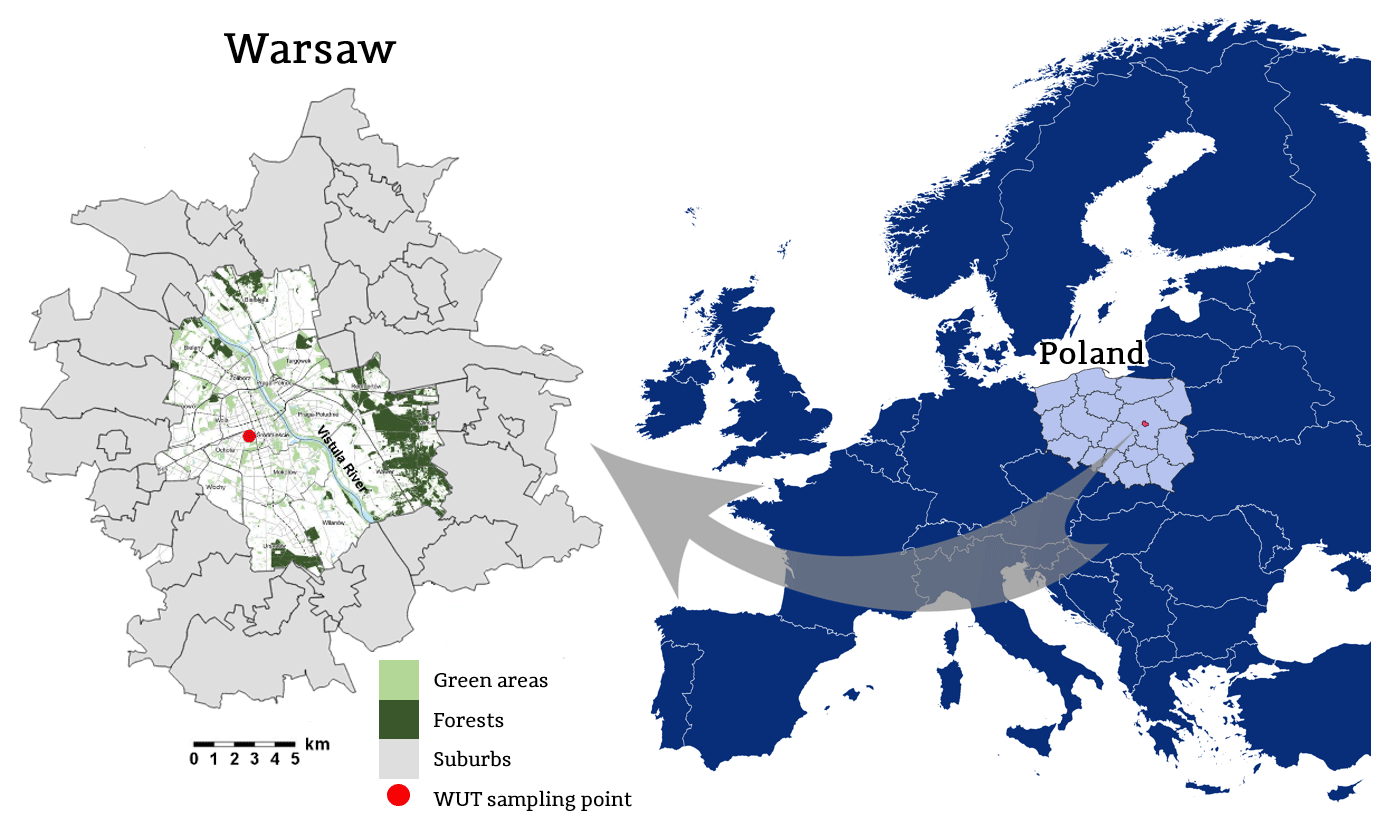
Figure 1 Location of the measurement site in Warsaw.

Warsaw is characterized by a moderately warm climate, with an annual mean temperature of 8.5 ^∘C and the annual sum of precipitation around 530 mm (data for 1986–2010)¹. January, with an average temperature of −1.9 ^∘C, and July, with an average temperature of 19.0 ^∘C, are the coolest and the warmest months, respectively. July is also characterized by the highest precipitation (72.9 mm), while in February the lowest precipitation is observed (26.1 mm).

During the measurement campaign, the mean values of temperature, relative humidity, air pressure, wind speed, predominant wind direction, and the sum of precipitation measured at the sampling site were 3 ^∘C, 87 %, 1009 hPa, 2  m s⁻¹, W and E, and 24 mm, respectively.

The ambient air quality in the city is determined primarily by road transport emissions. Warsaw is characterized by a dense road network, with a total length of more than 2800 km, as well as the highest number of cars per 1000 inhabitants in the country, which equals 750. At the same time, frequent congestion is also observed in the city. The municipal economy is not focused on industrial production, but several point emission sources are located within the city, including two coal-fired combined heat and power plants, namely Siekierki (heat capacity 2078 MW_thheat capacity 620 MW_e) and Żerań (heat capacity 1280 MW_thheat capacity 373 MW_e), as well as a steel plant with an annual production of 600 000 t of steel products. Warsaw has the largest central heating supply system in the European Union, with a network of over 1800 km, covering roughly 80 % of the city's heat demand. However, the city is surrounded by numerous smaller suburbs dominated by individual household heating, mainly using solid fuels (coal and wood) and gas but also solid fuels of very low-quality, such as used engine oil and waste (see, e.g., Juda-Rezler et al., 2021).

In order to choose the location of the sampling site, which would be representative for the urban background concentrations, air pollution dispersion modeling by the CALMET/CALPUFF system has been carried out (see Maciejewska, 2020). The site of the Warsaw University of Technology (WUT) was placed in the city center, within a 34 ha area of the city's water treatment station, and was beyond the direct influence of any particular local emission source or traffic.

2.2 PM sampling and elements determination

The sampling campaign was carried out during winter, between 18 February and 10 March 2016. The aerosol was collected by a sampling device (Pixe International Corporation; Calzolai et al., 2015) designed to separate the fine (< 2.5 µm aerodynamic diameter) and the coarse (2.5–10 µm aerodynamic diameter) modes of atmospheric aerosol at an airflow rate of 1 L min⁻¹. Coarse particles are collected on an impaction surface made up of an Apiezon-coated polypropylene foil, whereas fine particles are collected on a Nuclepore filter. The two collecting substrata are paired on a cartridge that rotates under the air inlet at constant speed for a week. Thus, on each one of the two stages, a circular continuous deposition of particulate matter (the streak) is formed; streaks are analyzed by means of the PIXE (particle-induced X-Ray emission) technique, using a scan system. The proton beam size for PIXE analysis, together with the pumping orifice width and the cartridge rotation speed, determine the time resolution on the elemental composition of PM, which is 1 h.

The PIXE measurements were performed at the Italian National Institute of Nuclear Physics (INFN) LABEC (Laboratorio di tecniche nucleari per l'Ambiente e i Beni Culturali – Laboratory of Nuclear Techniques for. Environment and Cultural Heritage) laboratory in Florence with a 2.7 MeV proton beam extracted from the 3 MV HVEE Tandetron accelerator. The external beam setup, fully dedicated to environmental analysis, is extensively described elsewhere (Lucarelli, 2020). As mentioned before, the deposit streak was analyzed point by point, with steps matching 1 h of sampling. Each point was irradiated for about 60 s with a 50–300 nA beam current. The PIXE spectra were fitted by means of the GUPIX code (Campbell et al., 2010), and elemental concentrations were obtained by a calibration curve from a set of thin standards of certified areal density (Micromatter Technologies Inc., Surrey, BC, Canada). Uncertainties of the hourly elemental concentrations result from the sum of independent uncertainties on the certified standards thickness (5 %), aerosol collection area (2 %), airflow (2 %), and X-ray count statistics (2 %–20 %). Indeed, concentration values near the minimum detection limits (MDLs) are characterized by higher uncertainties. Typical detection limits range from about 10 ng m⁻³ for low Z elements down to 1 ng m⁻³ (or below) for medium–high Z elements. The following 27 elements for a total sampling time of 500 h were detected in both fractions: Na, Mg, Al, Si, P, S, Cl, K, Ca, Ti, V, Cr, Mn, Fe, Ni, Cu, Zn, As, Se, Br, Rb, Sr, Y, Zr, Mo, Ba, and Pb.

Simultaneously with the streaker measurement campaign, daily concentrations of PM_2.5 mass and its chemical composition, including EC (elemental carbon), OC (organic carbon), water-soluble inorganic ions, i.e., ${{\mathrm{NO}}_{\mathrm{3}}}^{-}$, ${{\mathrm{SO}}_{\mathrm{4}}}^{\mathrm{2}-}$, ${{\mathrm{NH}}_{\mathrm{4}}}^{+}$, Cl⁻, Na⁺, K⁺, Ca²⁺, and Mg²⁺, were measured. PM_2.5 concentrations were determined according to the EN 12341:2014-07 standard (i.e., Ambient air – Standard gravimetric measurement method to determine the concentration of mass fractions PM₁₀ or PM_2.5 particulate matter). EC and OC content was determined with the use of a Sunset Laboratory thermal-optical carbon aerosol analyzer, equipped with a flame ionization detector, using the EUSAAR_2 protocol (Cavalli et al., 2010), while the ionic constituents were determined with the use of ion chromatography (Dionex ICS-1100, Thermo Scientific Inc., USA; see Juda-Rezler et al., 2020).

2.3 Positive matrix factorization

Positive matrix factorization (PMF) was applied to the hourly data sets (independently for fine and coarse fractions), allowing for the identification of the major PM sources in both modes. In this study, the EPA PMF 5.0 software was used. PMF is a widely used (e.g., Belis et al., 2020; Hopke et al., 2020) multivariate factor analysis model in air quality studies based on a weighted least squares fit approach (Paatero and Tapper, 1994). It uses the uncertainties of each measurement to weigh the individual data points and imposes non-negativity constraints in the optimization process. In the PMF modeling procedure, a matrix of the measurement data (X) is decomposed into two matrices to be determined, namely factor contributions (G) and factor profiles (F), as indicated in Eq. (1) as follows (Paatero and Tapper, 1994):

$$\begin{array}{}\text{(1)}& \mathbf{X}=\mathbf{G}\cdot \mathbf{F}+\mathbf{E},\end{array}$$

where X, G, and F are the n×m matrix of the measurement data of m chemical species in n samples, n×p matrix of p sources' contribution, and p×m matrix of profiles of p sources, respectively, while E is the residual matrix.

The mass balance equation (Eq. 1) is solved in PMF by minimizing the object function Q given by Eq. (2), as follows (Paatero, 1997):

$$\begin{array}{}\text{(2)}& Q={∥{\displaystyle \frac{(\mathbf{X}-\mathbf{G}\cdot \mathbf{F})}{\mathit{\sigma }}}∥}_F^{\mathrm{2}},\end{array}$$

where σ is the matrix of known uncertainties for the measurement data.

According to the procedure of the preparation of the input data proposed by Polissar et al. (1998), concentrations of elements below the detection limit (DL) were replaced with the values of one-half of the DL, and their uncertainties were set at five-sixths of the DL values, while missing data were substituted by the geometric mean of the concentrations, with uncertainties set at 4 times of the geometric mean concentration. The signal-to-noise (S$/$N) criterion (Paatero and Hopke, 2003) was applied to input data in order to separate the variables that retained a significant signal from that dominated by noise. Species with $\text{S}/\text{N}>\mathrm{2}$ were defined as strong variables and, used in PMF as they are, species with $\mathrm{0.2}<\text{S}/\text{N}<\mathrm{2}$ were classified as weak variables and downweighted by a factor of 3, while species with $\text{S}/\text{N}<\mathrm{0.2}$ were considered as being bad variables and removed from the analysis. A criterion of the share of data above the DL was also used (Amato et al., 2016; Cesari et al., 2018). Finally, PMF was applied to 20 elements in 500 samples and 22 elements in 492 samples in the case of fine and coarse fractions, respectively. Based on the S$/$N ratio, most of the elements were considered as being good variables, except P, Cr, As, Se ,and Sr in the fine fraction and P, As, Br, Zr, Ba, and Pb in the coarse fraction, which were classified as weak variables.

A number of solutions with 3 to 10 resolved factors were tested to find out the most optimal one. In order to examine the quality of the obtained solution, several criteria were applied, including the extraction of realistic source profiles, the distribution of scaled residuals, and the comparison between the modeled and observed mass of elements. The best solution was obtained using seven factors and five factors in the fine and coarse fractions, respectively, representing a reasonable physical interpretation of the sources, with the measured total concentration of elements reproduced well (with R²=0.96 for the fine fraction and R²=0.99 for the coarse fraction). Almost all variables showed scaled residuals estimated by PMF between −3 and +3. The bootstrapping method applied with 100 runs and minimum correlation R value of 0.6 revealed a stable PMF solution.

In this study, concentrations of PM mass and its macro components, i.e., organic carbon, elemental carbon, secondary inorganic aerosols, and other water-soluble inorganic ions, were not available with the hourly temporal resolution. Therefore, the analysis of the hourly concentrations of the elements was used for the detailed identification of PM sources, supplementing the previous source apportionment study performed by Juda-Rezler at al. (2020). Due to the lack of PM mass in the measurement campaign, the contribution of the identified sources to the total aerosol mass cannot be provided, and the source time series will be expressed in arbitrary units (see, e.g., Lucarelli et al., 2020).

2.4 Conditional probability function analysis

The conditional probability function (CPF) is a technique commonly used to identify the contributions of local and regional sources affecting a given monitoring site and the relationship between air pollutant concentrations and wind speed. Bivariate polar plots are used to illustrate the results of the CPF, which calculates the probability that the concentration of a given species is greater than a specified value, usually expressed as a high percentile of the concentrations, as a function of both wind speed and direction, according to Eq. (3) as follows (Uria-Tellaetxe and Carslaw, 2014):

$$\begin{array}{}\text{(3)}& {\text{CPF}}_{\mathrm{\Delta }\mathit{\theta }}={\displaystyle \frac{m_{\mathrm{\Delta }\mathit{\theta }}{\mathrm{|}}_{C\ge x}}{n_{\mathrm{\Delta }\mathit{\theta }}}},\end{array}$$

where m_Δθ is the number of samples in the wind sector θ, with concentration C greater than or equal to a threshold value x, and n_Δθ is the total number of samples from wind sector Δθ. Thus, CPF indicates the potential for a source region to contribute to high air pollution concentrations (Uria-Tellaetxe and Carslaw, 2014).

In this study, all CPF analyses were performed in the openair R package (Carslaw and Ropkins, 2012) and were applied to the PMF source factors, assuming the 90th percentile of the concentrations as a threshold value.

2.5 Air mass back trajectory clustering

The HYbrid Single-Particle Lagrangian Integrated Trajectory (HYSPLIT) model of the NOAA Air Resources Laboratory (Draxler and Hess, 1998) was applied to compute 96 h air mass backward trajectories starting at 200 m a.s.l. (above sea level) over the sampling site for each hour of the analyzed period. Meteorological fields from the ERA-Interim reanalysis (Dee et al., 2011) of the European Centre for Medium-Range Weather Forecasts (ECMWF) were formatted to be used as input data for the HYSPLIT runs. The 6 h data are gridded in 27 pressure levels from 1000 up to 100 hPa and were bilinearly interpolated to 0.5^∘ horizontal resolution to take advantage of the 0.5^∘ model's terrain.

The trajectories were classified into homogeneous groups by a non-hierarchical clustering procedure based on the k-means algorithm, which groups a given data set into a number of clusters, k, fixed a priori, assigning each case to the best-fitting cluster. Each cluster is represented by its centroid, i.e., the average over the trajectories belonging to it. Initially, k starting centroids are set randomly with all trajectories allocated into the clusters of their nearest centroid. The centroids are then recalculated by averaging all the trajectories belonging to the same cluster in an iterative process until the cluster assignments no longer change. As the final clusters produced by the k-means algorithm are sensitive to the selection of initial centroids, for a given k the clustering procedure was repeated 800 times in order to identify stable centroid positions and provide more robust results (Orza et al., 2012). The haversine formula of the great circle distance between two points (Sinnott, 1984) given by Eq. (4) was used as the similarity measure in the clustering process, as follows:

$$\begin{array}{ll}{\displaystyle }D=& {\displaystyle }\mathrm{2}{R}_{\mathrm{E}}{\sin }^{-\mathrm{1}}\left(\left[{\sin }^{\mathrm{2}}\left({\displaystyle \frac{{\mathit{\phi }}_{\mathrm{1}}-{\mathit{\phi }}_{\mathrm{2}}}{\mathrm{2}}}\right)\right.\right.\\ \text{(4)}& {\displaystyle }& {\displaystyle }\left.{\left.+\cos {\mathit{\phi }}_{\mathrm{1}}\cos {\mathit{\phi }}_{\mathrm{2}}{\sin }^{\mathrm{2}}\left({\displaystyle \frac{{\mathit{\lambda }}_{\mathrm{1}}-{\mathit{\lambda }}_{\mathrm{2}}}{\mathrm{2}}}\right)\right]}^{\mathrm{1}/\mathrm{2}}\right),\end{array}$$

where D is the distance between two points of the Earth (kilometers), φ₁, and φ₂ are their latitudes (radians), λ₁ and λ₂ are their longitudes (radians), and R_E is the Earth radius (6367.45 km). The total distance between a trajectory i and a cluster centroid c is then as follows:

$$\begin{array}{}\text{(5)}& D_{i,c}=\sum _{s=\mathrm{1}}^{N_s}{D}_{i,c,s},\end{array}$$

where $D_{i,c,s}$ is the distance between the points of back trajectory i and centroid c at the time step s, calculated with Eq. (4), and the summation runs over the total number of backward time steps. The score function that measures the quality of the clustering is the total within-cluster root mean squared distance (RMSD) between individual trajectories and their centroids, as follows:

$$\begin{array}{}\text{(6)}& {\text{RMSD}}_c=\sqrt{{\displaystyle \frac{\mathrm{1}}{N_c}}\sum _{i=\mathrm{1}}^{N_c}{D}_{i,c}^{\mathrm{2}}},\end{array}$$

$$\begin{array}{}\text{(7)}& {\text{RMSD}}_{\text{total}}=\sum _{c=\mathrm{1}}^k{\text{RMSD}}_c,\end{array}$$

with N_c being the number of trajectories belonging to cluster c, and k is the number of clusters. The optimal number of clusters was assessed following a procedure similar to that of Dorling et al. (1992). The number of clusters k was successively reduced by one, from 30 down to 3 clusters, and the total within-cluster RMSD between individual trajectories and their centroids given by Eqs. (6) and (7) was examined as a function of the number of clusters. The optimal number of clusters is, finally, the lowest number of clusters for which the lowest percentage change in RMSD_total is found when decreasing k by one.

3 Results and discussion

3.1 Daily PM_2.5 composition and meteorological conditions

Simultaneous to the streaker data collection, daily concentrations of PM_2.5 and its components were collected. Daily elemental concentrations (averaged from the hourly data) and daily concentrations of the respective water-soluble ions (${{\mathrm{SO}}_{\mathrm{4}}}^{\mathrm{2}-}$, K⁺, Cl⁻, and Na⁺) were compared. A general good agreement was found, with a strong correlation between elemental sulfur and ${{\mathrm{SO}}_{\mathrm{4}}}^{\mathrm{2}-}$ (r=0.97), as well as between elemental and water-soluble potassium (r=0.74). For elemental and water-soluble chlorine and sodium, moderate correlations (r=0.69 and r=0.61, respectively) were observed. Calcium and magnesium concentrations could not be compared due to missing data and data below the detection limit.

The time series of daily concentrations of the main components of PM_2.5 throughout the measurement period (18 February–10 March 2016) are presented in Fig. 2.

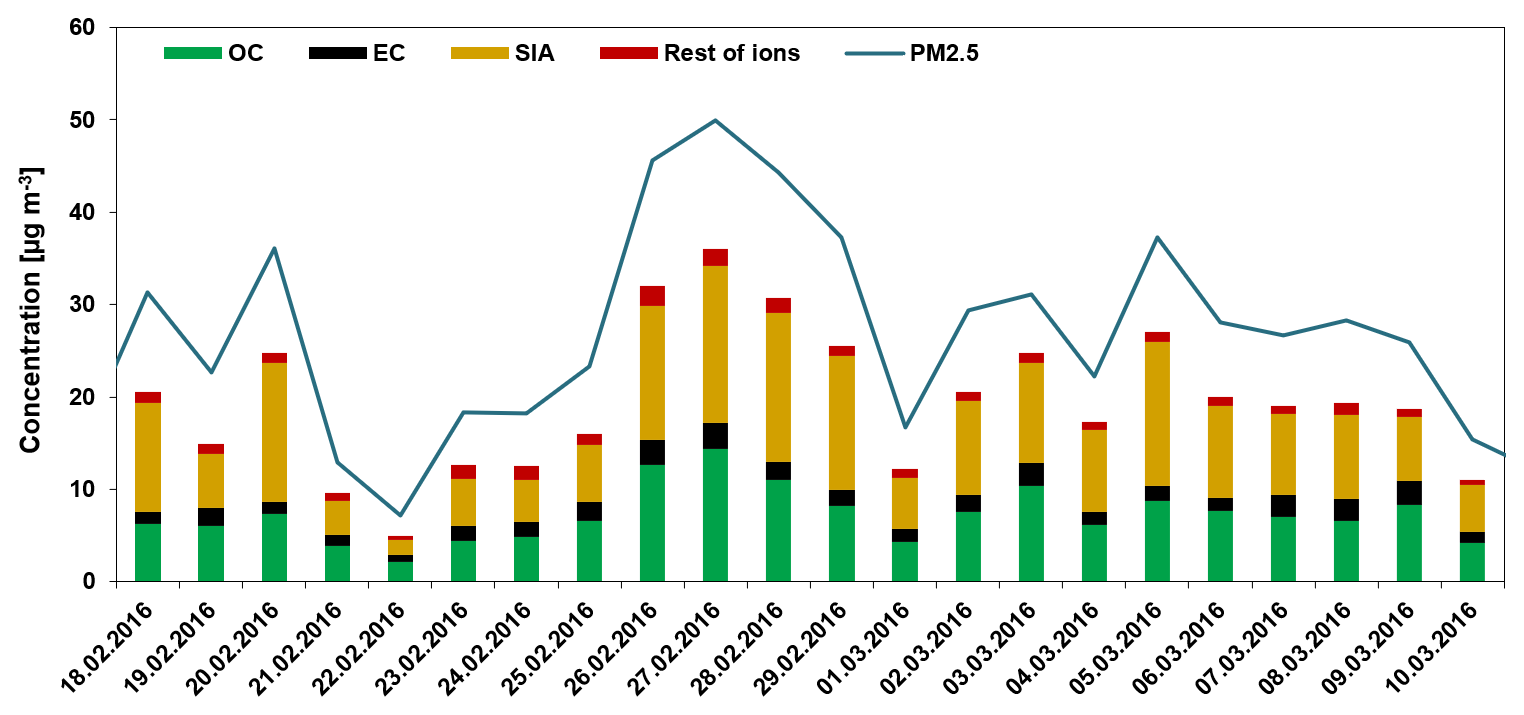
Figure 2 Time series of daily concentrations (micrograms per cubic meter; hereafter µg m⁻³) of PM_2.5 (line) and its main components (bars) in Warsaw in the sampling period from 18 February to 10 March 2016. The rest of the ions indicate the sum of concentrations of the K⁺, Cl⁻, Na⁺, Mg²⁺, and Ca²⁺ ions.

Mean PM_2.5 mass concentration in the measurement period equaled 27.7 µg m⁻³ (SD=11.0 µg m⁻³), which is almost 50 % higher that the annual mean PM_2.5 concentration observed in the whole of 2016 (18.8 µg m⁻³). The highest value of 49.9 µg m⁻³ was recorded on 27 February, exceeding the WHO daily air quality guideline (25 µg m⁻³) almost twice. The main components of fine particulate matter in Warsaw were secondary inorganic aerosols (SIAs; the sum of ${{\mathrm{SO}}_{\mathrm{4}}}^{\mathrm{2}-}$, ${{\mathrm{NO}}_{\mathrm{3}}}^{-}$, and ${{\mathrm{NH}}_{\mathrm{4}}}^{+}$) and organic carbon, accounting for 35 % and 26 % of the PM_2.5 mass, respectively. SIAs and OC exhibited higher and lower content, respectively, compared to their contributions in PM_2.5 during the whole of 2016, which, in both cases, reached on average about 30 % of the fine fraction (see Juda-Rezler et al., 2020). At the same time, the contribution of these components exceeds their typical content in PM_2.5 mass reported for urban background sites in Southern and Central Europe (see, e.g., Amato et al., 2016; Błaszczak et al., 2019). Among SIAs, the highest share was observed for ${{\mathrm{SO}}_{\mathrm{4}}}^{\mathrm{2}-}$ (17 % and 49 % in PM_2.5 and SIA mass, respectively), followed by ${{\mathrm{NO}}_{\mathrm{3}}}^{-}$ (12 % and 34 %) and ${{\mathrm{NH}}_{\mathrm{4}}}^{+}$ (6 % and 17 %). The share of the remaining PM_2.5 components was much smaller, as EC constitutes about 6 % and inorganic ions other than SIAs (K⁺, Cl⁻, Na⁺, Mg²⁺, Ca²⁺) constitute around 4 % of PM_2.5. As reported by Juda-Rezler et al. (2020), in the heating season during which the streaker measurement campaign was carried out, a remarkable increase in the concentrations of OC, EC, ${{\mathrm{NO}}_{\mathrm{3}}}^{-}$, ${{\mathrm{NH}}_{\mathrm{4}}}^{+}$, and Cl⁻ was observed in comparison to other seasons.

3.2 Hourly elemental composition

The descriptive statistics for the hourly concentrations of 27 analyzed elements measured in both size fractions are given in Table 1.

Table 1 Descriptive statistics for the hourly concentrations (nanograms per cubic meter; hereafter ng m⁻³) of the elements measured in the fine and coarse fractions. Minimum concentrations below the detection limit are indicated by an asterisk.

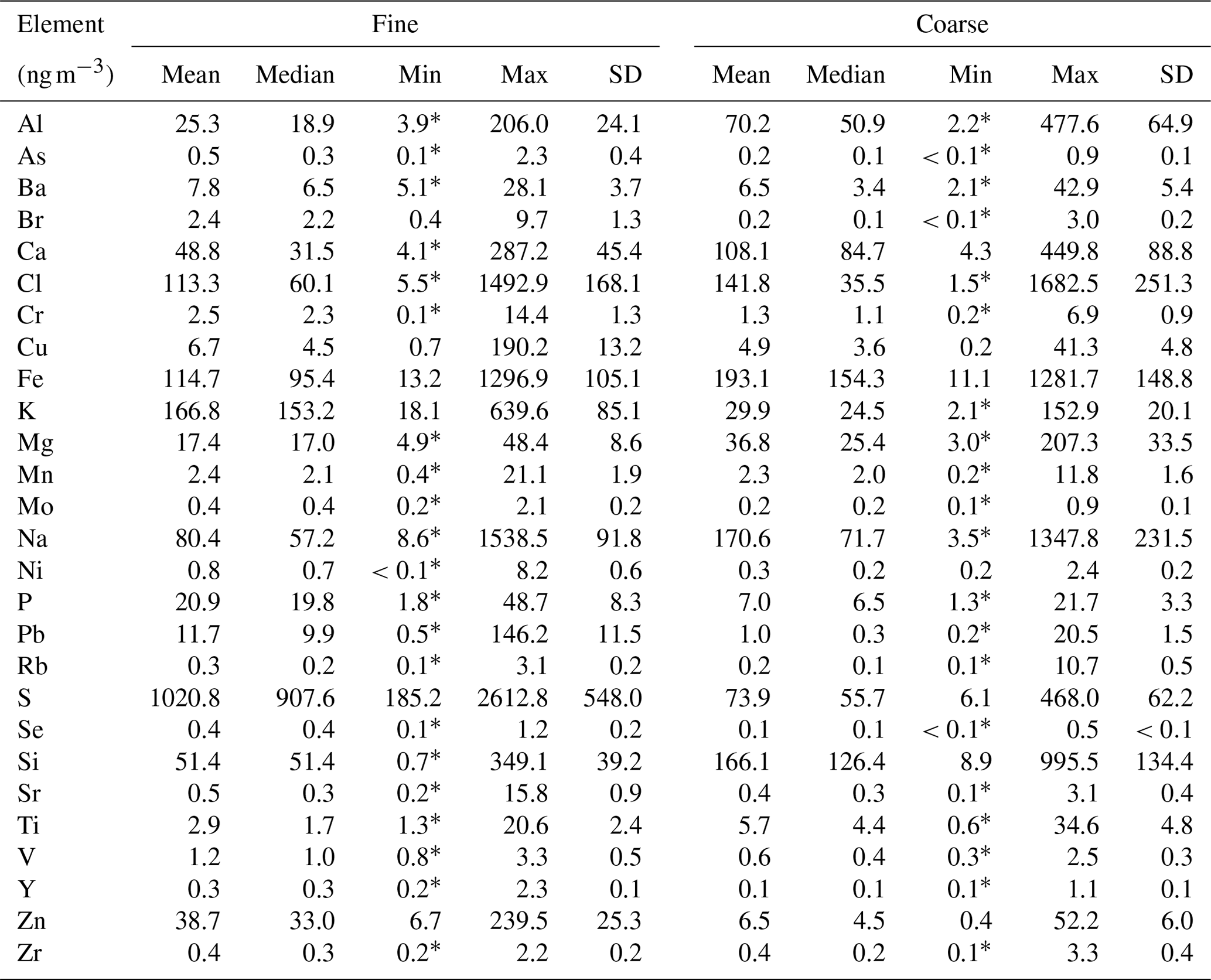
In terms of PM₁₀ (the sum of the fine and coarse fractions), S (1095 ng m⁻³) is found to be the most abundant element, followed by Fe (308 ng m⁻³), Cl (255 ng m⁻³), Na (251 ng m⁻³), Si (218 ng m⁻³), K (197 ng m⁻³), and Ca (157 ng m⁻³). Concentrations lower than 1 ng m⁻³, and in some cases below the detection limits, are observed for As, Mo, Rb, Se, Sr, Y, and Zr. The measured elements may be divided into three groups according to their presence in the respective fraction. The first group represents the elements which are abundant mainly in the fine fraction, with both mean and median values substantially higher than in the coarse one. These are As, Br, Cr, Cu, K, Mo, Ni, P, Pb, S, Se, V, Y, and Zn and all of them are typically emitted by fuel combustion and road traffic (e.g., Belis et al., 2013). Metals are primarily of crustal or marine origin; i.e., Al, Ca, Fe, Mg, Na, Si, and Ti belong to the second group of elements distributed mainly in the coarse fraction. A different behavior is observed for Cl, the content of which in the coarse fraction is characterized by a higher mean value but a lower median value compared to the fine fraction. In the third group, the concentrations of Ba, Mn, Rb, Sr, and Zr, which are the elements related to such abrasion processes as tire and brake wear (Pant and Harrison, 2013), are balanced between the two fractions.

The hourly time resolution of the elements measured in the fine and coarse fractions allowed us to follow the diurnal evolution of primary PM sources activity and the formation of secondary aerosol in detail. The analysis of the concentration time series revealed differences between the two fractions for most of the elements. As an example, the temporal trends of selected elements contained in both fractions are shown in Fig. 3, while the trends for the rest of the elements are given in the Supplement (Figs. S1–S23). The following paragraphs present the discussion of the time series of four selected elements, the concentrations of which display various patterns and help in distinguishing and identifying PM emission sources.

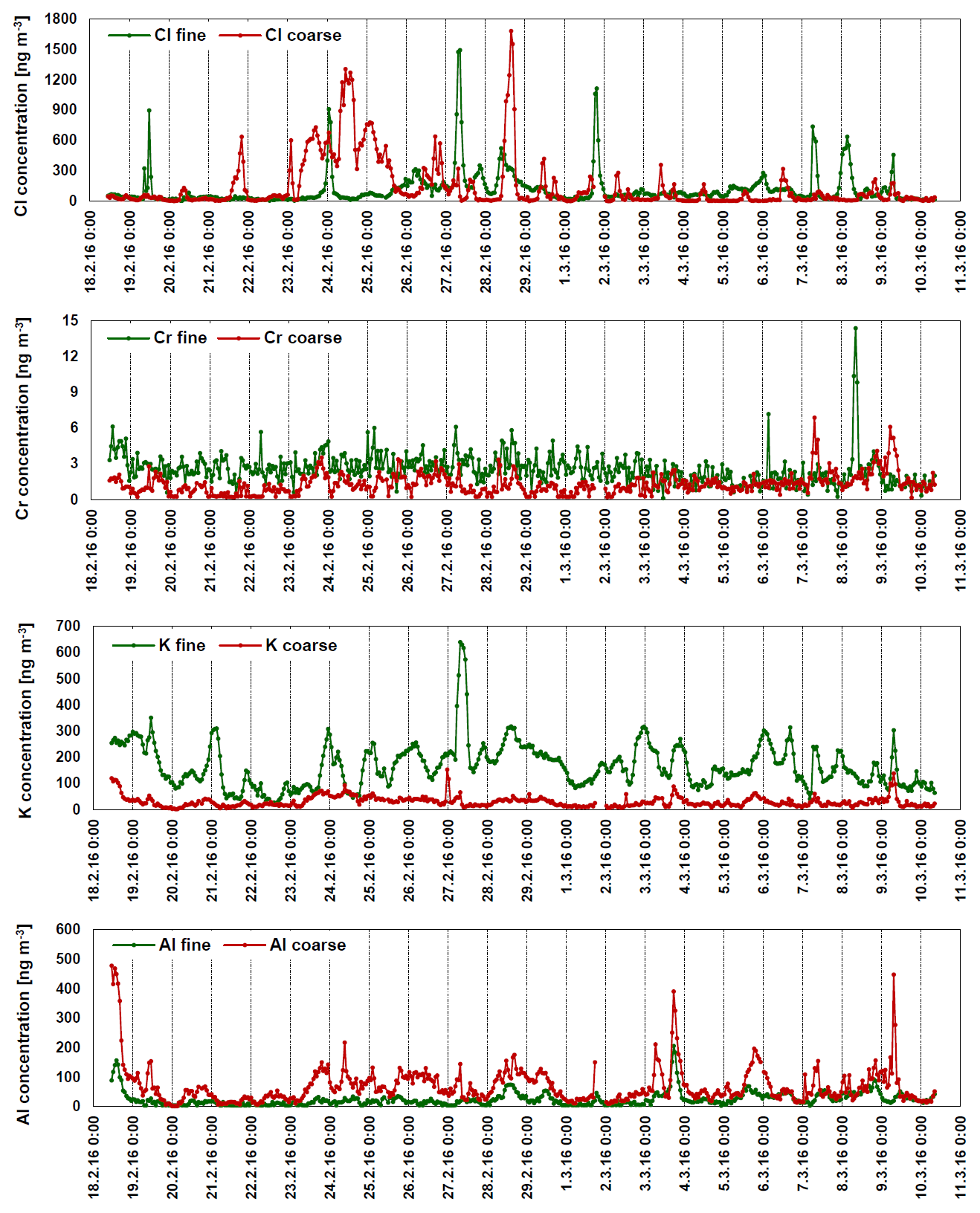
Figure 3 Hourly concentrations (ng m⁻³) of Cl, Cr, K, and Al measured in the fine (green) and coarse (red) fractions.

Cl is usually attributed either to sea salt in areas close to the coast or to road salt in continental areas of central and northern Europe (Belis et al., 2013). It is also emitted from the combustion of coal, wood, and solid waste, in particular in the residential sector (e.g., Mikuška et al., 2020). The recorded time series of Cl in Warsaw are different in the fine and coarse fractions, with no correlation between the concentrations in the two modes (r=0.08). In the coarse fraction, Cl is mainly correlated with other markers of road salt, i.e., Na (r=0.96) and Mg (r=0.78), while in the fine fraction Cl is not correlated with other elements (r=0.02–0.44), with the exception of Br and K, for which moderate correlations (r=0.69 and r=0.54, respectively) are observed. The concentrations of Cl are higher in the coarse fraction, with a mean level of 142 ng m⁻³ and several peak values up to almost 1700 ng m⁻³, while in the fine fraction the mean Cl level reaches 113 ng m⁻³, with peaks up to almost 1500 ng m⁻³ (Fig. 3). In the coarse fraction, a strong increase in Cl is always present together with Na and Mg peaks, while in the fine fraction, during every increase in Cl the increase in concentrations of diverse elements is observed, and most often it is accompanied by a slight increase in the concentrations of Br, K, or different crustal elements. The temporal trend of Cl in the coarse fraction is characterized by peaks in the morning (between 06:00 and 08:00 UTC; universal coordinated time is given hereafter, unless indicated otherwise) and evening (between 17:00 and 23:00). In contrast, there is no clear daily pattern of Cl in the fine fraction, where the peaks of elevated concentrations last a few hours and occur on different days of the week and at different times of the day (Fig. 3). This suggests a different origin of Cl in both fractions.

There is also no correlation between the concentrations in the two fractions (r=0.04) in the case of Cr, which is generally associated with industrial or vehicular emissions (e.g., Taiwo et al., 2014; Banerjee et al., 2015), but also with coal burning in small domestic boilers (Juda-Rezler et al., 2011). In the fine fraction, Cr is moderately correlated with Ni (r=0.56). For other elements, a weak correlation or no correlation was observed, yet the highest r values were obtained for other markers of industrial activities, i.e., Fe (r=0.49), Mn (r=0.42), and Mo (r=0.41). In the coarse fraction, Cr is strongly correlated with Fe (r=0.82), Mn (r=0.77), and Cu (r=0.75) and moderately with other traffic-related elements, i.e., Ba (r=0.68), Zn (r=0.50), and Ni (r=0.50), as well as with crustal elements such as Si (r=0.59), Ca (r=0.57), and Ti (r=0.52). This may suggest an industrial and traffic origin of Cr in the fine and coarse fractions, respectively. Concentrations of Cr are almost 2 times higher in the fine fraction (mean value of 2.3 ng m⁻³) than in the coarse one (1.3 ng m⁻³). As can be seen in Fig. 3, concentrations of Cr in the fine fraction show no diurnal variation and display several peaks up to 14.4 ng m⁻³, while in the coarse fraction, a bimodal diurnal cycle with typical peaks in the traffic rush hours from 06:00 to 10:00 and from 15:00 to 21:00 is observed.

Unlike the two aforementioned elements, a weak correlation between the concentrations in the fine and coarse fractions (r=0.40) is observed for K, which is present in mineral, dust but is also a typical marker of biomass burning (e.g., Nava et al., 2015). Concentrations of K are substantially higher in the fine fraction (mean value of 167 ng m⁻³) than in the coarse one (30 ng m⁻³). In the fine fraction, K is moderately correlated with elements recognized as markers of coal and wood combustion (e.g., Belis et al., 2013; Nava et al., 2015), i.e., Br (r=0.62), Se (r=0.60), Zn (r=0.58), S (r=0.55), and Cl (r=0.54). In addition, the diurnal cycle of concentrations of K in this fraction is characterized by peaks in the morning and evening hours (Fig. 3), which clearly points to solid fuels combustion in the residential sector. In the coarse fraction, K is mainly correlated with typical crustal elements, showing a strong correlation with Al (r=0.81), Si (r=0.80), and Ti (r=0.76) and a moderate correlation with Ca (r=0.69), Sr (r=0.63), Fe (r=0.62), and Mg (r=0.60). There is no clear daily variation in K in this fraction; however, daytime concentrations slightly exceed nighttime levels, which is likely related to the resuspension of mineral dust during daytime activities. Several peaks of concentrations of K, which are always present together with other crustal elements, are present during the measurement period.

A completely different behavior can be observed for Al, which, along with Ca, Fe, Mg, Si, Sr, and Ti, is a typical marker of mineral dust (e.g., Banerjee et al., 2015). Concentrations of Al are almost 2.5 times higher in the coarse fraction (mean value of 70 ng m⁻³) than in the fine one (25 ng m⁻³). A strong correlation between the concentrations in the fine and coarse fractions (r=0.70) is observed for this element. Moreover, in both modes, Al is correlated only with crustal elements, i.e., Ti (r=0.81), Si (r=0.63), and Ca (r=0.51) in the fine fraction, as well as Si (r=0.92), Ti (r=0.89), K (r=0.81), Ca (r=0.65), Sr (r=0.62), and Fe (r=0.55) in the coarse one. There is also a similar diurnal variation in both fractions, with Al concentrations higher during the daytime than at night. Most of the peak values of Al are present in both modes at the same time (Fig. 3) and occur together with other crustal elements, which suggests a crustal origin of the element in both fractions.

3.3 PM source apportionment

As described in Sect. 2.3, a solution with seven and five factors was chosen for the fine and coarse fractions, respectively. The identified source profiles, together with the daily patterns of the sources, are shown in Figs. 4 and 5. The following similar sources were observed in both fractions: sulfates, soil dust, road salt, and traffic- and industry-related sources, while Cl-rich and wood and coal combustion sources were identified only in the fine fraction. A detailed description of the identified sources is presented in the following (Sects. 3.3.1–3.3.7).

Figure 4 The left column shows the PMF profiles (bars; left y axis) and contributions (black diamonds; right y axis) of the identified sources for the fine fraction. The right column shows the daily patterns of the identified sources (in arbitrary units).

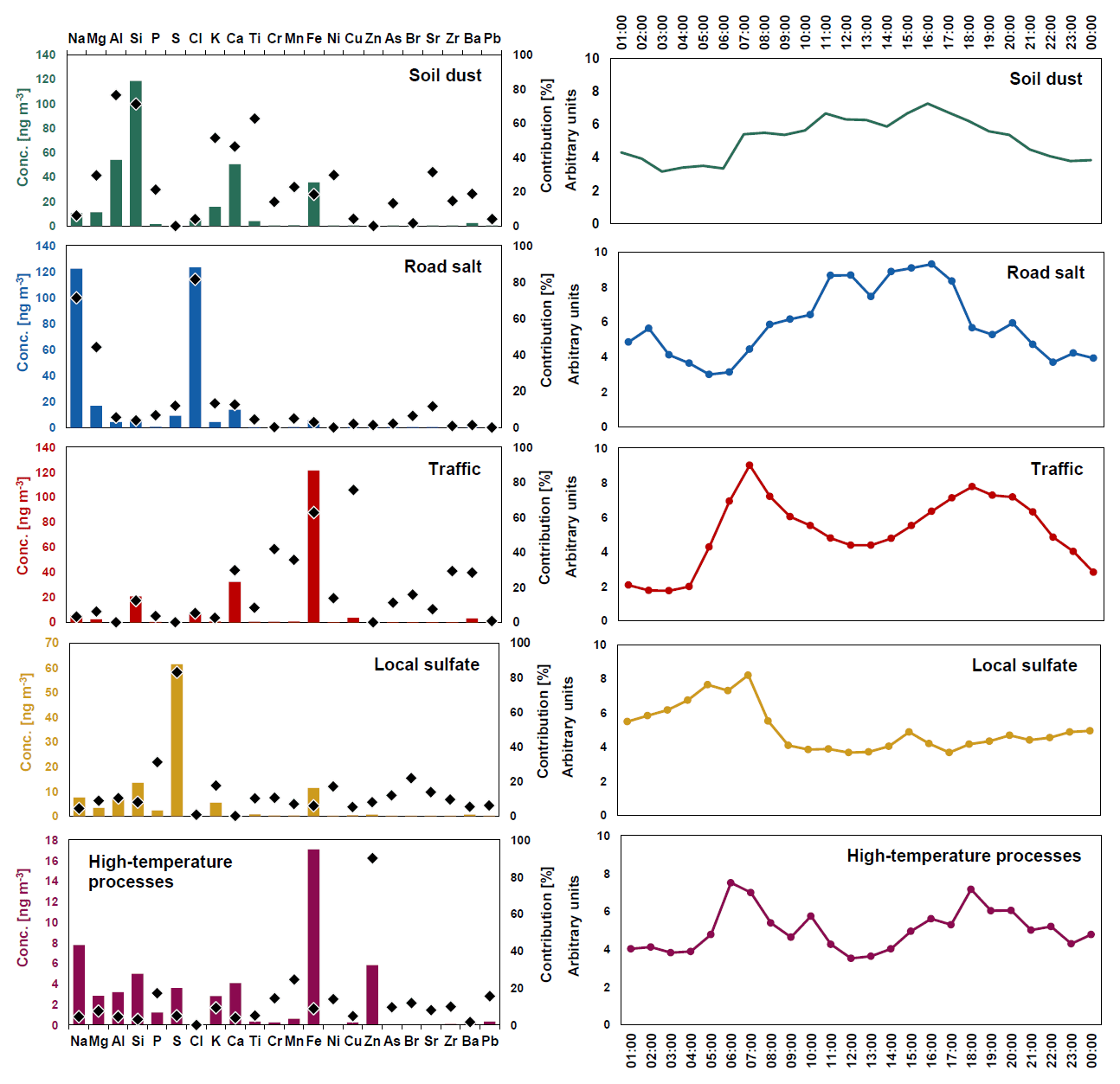
Figure 5 The left column shows the PMF profiles (bars; left y axis) and contributions (black diamonds; right y axis) of the identified sources for the coarse fraction. The right column shows the daily patterns of the identified sources (in arbitrary units).

For a better interpretation of the identified sources, polar plots of CPF analysis, combining PMF results with wind speed and direction, are presented in Fig. 6.

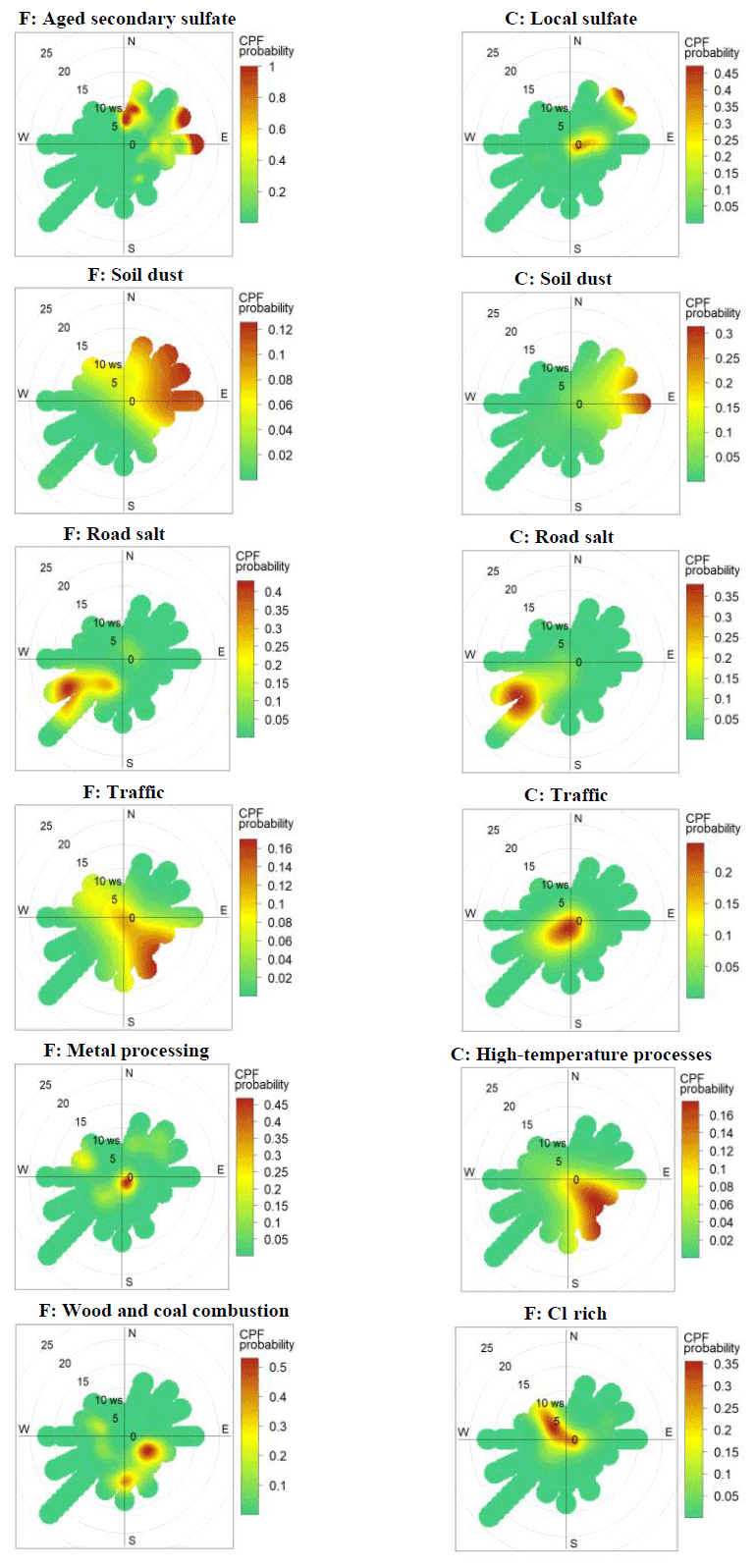
Figure 6 Conditional probability function (CPF) analysis (at the 90th percentile) of the PMF sources identified in the fine (F) and coarse (C) fractions. Wind speed (ws) is expressed in kilometers per hour (hereafter km h⁻¹).

3.3.1 Sulfates

In both fractions, the factor is characterized by high contributions of sulfur, representing 67 % and 83 % of the total mass of S in the fine and coarse fractions, respectively (Figs. 4 and 5). In addition, in the fine fraction, the factor is associated with notable loadings of P (30 % of P mass), Ni (23 %), and K (22 %) and, to a lesser extent, of Se and Br (around 15 % of the elements' mass). In the coarse fraction, the factor exhibits a similar profile with notable loadings of P (31 %), Br (23 %), K (18 %), and Ni (17 %). Se in this fraction was excluded from the PMF analysis as having the S$/$N ratio <0.2 (see Sect. 2.3); however, 12 % of the total mass of another marker of coal combustion (As) appears in the source profile. It is noteworthy that, in wintertime in Warsaw, As and K appeared to be highly bioavailable, indicating a high degree and rate of absorption of a substance by living systems or a high degree to which the substance is available to physiologically active sites. During the days of elevated air pollution levels, a higher bioavailability of those element was observed, suggesting a higher risk to humans posed by emissions from this source during those days (Juda-Rezler et al., 2021).

The presence of sulfur is associated with a secondary component produced by combustion processes of sulfur-containing fossil fuels. In the case of this study, its most probable source is domestic heating, emitting a substantial amount of SO₂, which in turn forms sulfate in the aqueous-phase conversion (Seinfeld and Pandis, 2016). All other elements related to this factor, and their mixture, have been previously attributed to small-scale residential combustion. K is a well-known marker of biomass burning, while Br may be produced by this type of sources as well (Nava et al., 2015). Also, a high contribution of P (together with K) has been previously attributed to wood combustion for heating purposes (Richard et al., 2011). Although As and Se are recognized as being markers of coal combustion in power plants (e.g., Banerjee et al., 2015), a substantial amount of these elements can also be released when coal is burned in the residential sector (IARC, 2012; Bano et al., 2018; Zhao and Luo, 2018). In turn, oil combustion constitutes the main source of Ni (e.g., Belis et al., 2013).

The S$/$K ratio can be used as an indicator to describe the rate of accumulation of S compounds in biomass burning aerosols during their transport. The ratios may range from 0.5, for fresh emissions, up to 8, for transported and aged aerosol (Viana et al., 2013, and references therein). The S$/$K ratios obtained in this study equal 6.1 and 2.5 for the fine and coarse fractions, respectively, pointing to aged fine aerosols and more freshly emitted coarse ones.

In general, secondary sulfate is primarily formed in the accumulation mode (particles with aerodynamic diameter 0.1–1 µm). Since secondary aerosol formation proceeds relatively slowly (in the time frame of hours and days), the daily source profile in the fine fraction does not exhibit a clear diurnal variation (Fig. 4). In the case of the coarse fraction, sulfate formation under nighttime condition of high relative humidity can play an important role. During the measurement period, the relative humidity was high, with average values of 89.4 % and 84.2 % at night and during the day, respectively. Under such conditions, SO₂ oxidation to sulfate occurs mainly on the particles with a water film surface or in the aqueous phase of particles. The oxidation is catalyzed by transition metals, in particular Fe and Mn (see, e.g., Sarangi et al., 2018; Wang et al., 2020). Therefore, the pattern of the source profile in this fraction is different than in the fine one, showing higher concentrations during late afternoon (around 15:00) and night (starting from 17:00), as well as nighttime contributions that are 2 times higher than those registered during the daytime (Fig. 5).

This confirms that the fine fraction is dominated by regional rather than local transport of SO₂ and sulfate from Warsaw's outskirts with small-scale residential combustion installations, mainly with the use of coal and biomass, whereas in the coarse fraction the presence of sulfate is probably due to the local combustion activities in the city itself. In addition, CPF analysis (Fig. 6) indicates the highest contributions at high wind speeds from regional sources to the north and east, where the small-scale combustion installations are located, but also from local sources in the case of coarse fraction. Thus, the source was recognized as being aged secondary sulfate and local sulfate for the fine and coarse fractions, respectively.

Overall, this source accounts for the highest contribution to the fine elemental mass (mean share during the measurement period equals 44 %) and a notable contribution to the coarse elemental mass (11.5 %). This result suggests that regional sources, including emissions from the residential sector located to the north and east of Warsaw, have a significant influence on the fine PM composition in the city. This is consistent with the conclusions of Juda-Rezler et al. (2020) who, based on the analysis of daily concentrations of PM_2.5 and its constituents measured in Warsaw for the whole 2016 year, found that fresh and aged aerosol from the residential sector transported from the outskirts of the city constitutes on average 45 % of PM_2.5 mass.

3.3.2 Soil dust

This factor, accounting for the highest contribution to the coarse elemental mass (31.5 %) and a notable contributor to the fine elemental mass (13.5 %), is characterized by contributions from typical crustal elements (e.g., Belis et al., 2013; Banerjee et al., 2015), i.e., Si (91 % of Si mass), Ca (71 %), Al (41 %), Fe (21 %), and Mg (19 %) in the fine fraction, as well as Al (77 %), Si (71 %), Ti (63 %), K (52 %), Ca (47 %), Sr (31 %), and Mg (29 %) in the coarse one. In addition, in the coarse fraction, along with crustal elements, notable contributions of species associated with traffic emissions (see Sect. 3.3.4), i.e., Ni (30 %), Mn (23 %), P (21 %), Ba (19 %), Zr (15 %), and Cr (14 %) are noted. Therefore, in this fraction, the source can be assigned to a mixed source consisting of soil dust with a substantial contribution of road dust.

The diurnal profiles in both size fractions have comparable patterns (Figs. 4 and 5), with substantially higher concentrations during the day (between 06:00 and 19:00); however, the peak values observed in the coarse fraction coincide with morning and afternoon traffic rush hours (07:00–08:00 and 16:00), confirming road dust as a contributing source. CPF analysis (Fig. 6) shows that, despite some differences in the source profile and the diurnal variation in both cases, the highest contributions come from the northeast, at high and moderate wind speeds, and from the east, at high wind speeds, suggesting similar source locations.

3.3.3 Road salt

This is the second-largest factor contributing to the coarse elemental mass (31 %), and a noticeable one in the case of the fine elemental mass (12.5 %), and it is characterized by high loading of elements attributed to road salt. During the measurement campaign, deicing salt, mainly composed of NaCl and/or MgCl₂, was applied on the roads in Warsaw. While Na and Mg have notable contributions in both fractions (71 % and 77 % Na and 44 % and 29 % Mg in the coarse and fine fraction, respectively), the two sources can be differentiated based on the level of Cl (Figs. 4 and 5). This factor reconstructs >80 % of Cl mass in the coarse fraction and only 5 % in the fine one, indicating fresh coarse and aged fine particles of road salt origin. The Cl depletion in the fine fraction is most probably caused by the well-known heterogeneous chemical reactions between NaCl and nitric (HNO₃) and sulfuric (H₂SO₄) acids, resulting in the formation of sodium nitrate and sodium sulfate, as well as in the volatilization of HCl (Seinfeld and Pandis, 2016). In addition, the factor in the fine fraction also includes notable contributions from elements usually associated with traffic emissions (P, Cr, Ni, and Br), which confirms the anthropogenic character of the source.

As can be seen in Fig. 5, in the coarse fraction, daytime levels exceed the nighttime ones with peak values observed in the morning and afternoon traffic rush hours (08:00–11:00 and 16:00), indicating that road salt is resuspended through daytime activities nearby the measurement site. In the fine fraction, the diurnal variation is less evident and less variable (Fig. 4); however, some peaks are observed in similar traffic rush hours (06:00–11:00 and a slight increase starting from 16:00), which may suggest that both local origin of the salt and its transport from distant roads nearby the city. CPF analysis (Fig. 6) indicates that the highest contributions of both source profiles come from the southwest at high and moderate wind speeds, and in addition, at lower wind speeds in the case of the coarse fraction, suggesting similar source locations. One of the main city roads and an expressway are located in this direction.

3.3.4 Traffic emissions

In the fine fraction, this factor, explaining 8 % of the elemental mass, is associated with high loadings of Fe (66 % of the Fe mass), Mn (42 %), Ni (28 %), Cr (21 %), and small amounts of Zn (14 %), Si (12 %), and Pb (9 %). In the coarse fraction, the factor contributes to the elemental mass in 20 % and is dominated by Cu and Fe, with 76 % and 63 % of the mass explained by these elements, respectively. High loadings of Cr (42 %), Mn (36 %), Ca (30 %), Zr (30 %), and Ba (28 %) and, to a lesser extent, of Br (16 %) and Ni (13 %) are present as well. Cu in the fine fraction appears not to be associated with traffic emissions (see Sect. 3.3.5). All the abovementioned elements may be emitted from abrasion of roads (Ca, Fe, Mn, and Si), brake linings and pads (Ba, Cu, Cr, Fe, Mn, Pb, and Zr), as well as of tires (Fe, Mn, and Zn; e.g., Pant and Harrison, 2013; Amato et al., 2014; Banerjee et al., 2015). Nevertheless, most of these elements can also be related to diverse exhaust-related emissions, i.e., fuel and lubricant combustion, catalytic converters, particulate filters and engine corrosion (Pant and Harrison, 2013, and references therein), while Ba can be emitted from gasoline, liquefied petroleum gas, and diesel engines. Ba and Zn have been reported to be strongly associated with diesel fuel, while Cu, Mn, and Sr with gasoline (Pant and Harrison, 2013). Fe, being a fuel additive, can be emitted from diesel engines (Bugarski et al., 2016). Thus, the factor in both fractions is likely to be attributed to the more general source, namely traffic, including both non-exhaust and exhaust emissions.

The factor in both modes displays a strong bimodal cycle that followed the peak times characteristic for traffic (Figs. 4 and 5). The highest levels are observed in the morning (between 06:00 and 10:00, with peaks at 07:00–08:00) and late afternoon and evening (between 15:00 and 21:00, with peaks at 18:00), although in the coarse fraction the second peak is less evident. CPF analysis (Fig. 6) shows that the highest source contributions for the two fractions come from different directions. For the fine fraction, the highest contributions come from the southeast at high and moderate wind speeds with lower probability for low wind speeds, corresponding with the locations of another main city's road, while the highest contributions for the coarse fraction come only at low wind speeds originating from nearby roads.

3.3.5 Industrial processes

Overall, this factor does not represent a significant emission source influencing the air quality in Warsaw, as it accounts for 2 % and 6 % of the total fine and coarse elemental mass, respectively. In the fine fraction, the factor is dominated solely by Cu (66 % of the Cu mass) and Pb (16 %), while over 90 % of the mass of Zn and non-negligible parts of mass of Mn (25 %), P (17 %), Pb (16 %), Cr (14 %), Ni (14 %), As (10 %), and Fe (10 %) are found in the coarse fraction. These elements are commonly recognized as being emitted from industrial processes, such as ferrous and non-ferrous metal processing and steel industries (e.g., Banerjee et al., 2015; Amato et al., 2016). In addition, As, Cu, Cr, and Sn (which was not determined in the present study) have been found as specific tracers of glassmaking emissions (Ledoux et al., 2017). As mentioned above, As is a well-known marker of coal combustion in the power industry.

No specific diurnal variation with episodic peaks at different times of the day can be seen for the fine mode (Fig. 4). The time series of the factor shows intense contribution of elevated concentrations occurring at night (between 01:00–04:00) and smaller peaks at 07:00 and 19:00. During the day, an almost stable pattern is observed. The nighttime peak is mainly the result of elevated values recorded on 24 February; however, the causes of this episode were not identified. The CPF analysis (Fig. 6) indicates two possible sources of the factor. The first one, having the highest contributions to peak levels, is located nearby the monitoring site and may be associated with welding activities carried out in the area of the water treatment station where the measurement site was located. Cu and Pb have been found among the main components of welding emissions (e.g., Golbabaei and Khadem, 2015). The second source, with a lower probability of high factor levels is related to moderate wind speeds and is situated in the northwest. One of the biggest Polish steelworks with an electric arc furnace is located in this direction, around 10 km from the sampling site. Steelworks can also be associated with substantial emissions of Cu and Pb (e.g., Yatkin and Bayram, 2008). Thus, the source can be classified as a mixed one and named metal processing.

The time series of the factor in the coarse fraction is characterized by a higher number of episodic peaks, also suggesting an industrial source (Fig. 5). Based on the high contributions of Zn and other industry-related elements, the source may be classified as industrial emissions from steelworks and/or glassworks. Some amounts of As may also suggest coal combustion in a power plant. The diurnal cycle also demonstrates clear peaks at 06:00, 10:00, and 18:00, which may also point to the influence from a traffic source; however, further separation of the sources was not possible. The CPF analysis (Fig. 6) shows the highest contributions from the southeast at high and moderate wind speeds. In this direction a combined heat and power plant is located within the city's borders. There are no industrial plants located southeasterly in Warsaw; however, at a distance of up to 100 km, at which coarse particles can be typically transported (Seinfeld and Pandis, 2016), some industrial facilities such as steelworks, glassworks, and another coal-fired power plant are located. Therefore, in this fraction the source can be classified as being high-temperature processes.

3.3.6 Wood and coal combustion

This factor, identified only in the fine fraction (Fig. 4), contributes 10 % to the elemental mass and is dominated by Zn (54 % of the Zn mass), Pb (48 %), and K (40 %), with smaller contributions of Se (23 %), Br (22 %), and As (10 %). As already mentioned, K is the major compound emitted from wood biomass combustion, while Br was also considered as a marker of this source (Nava et al., 2015). Yet, when bark and waste wood or wood pellets are burned, besides K, also high amounts of Zn, Pb, and As are generated (Nava et al., 2015; Vicente et al., 2015). On the other hand, since As and Se are well-known markers of coal combustion in the power industry, the biomass co-firing with coal in large point sources cannot be excluded. Therefore, this factor can be classified as being mixed wood and coal combustion.

The temporal trend of this source follows the typical daily pattern of fuel combustion for heating purposes with maximum concentrations in the morning and evening, as well as at night when heat demand is the highest (Fig. 4), supporting its interpretation as a mixed wood and coal combustion for residential heating. The CPF analysis (Fig. 6) points towards two possible sources of the factor. The first one shows the highest contributions to peak levels from the southeast at moderate wind speeds. In this direction, a combined heat and power plant co-firing hard coal and wood biomass is located. Moreover, in this plant a new biomass-fired boiler, with the wood biomass as basic fuel, was commissioned in 2016, and during the measurement period, the boiler trial operation was carried out. The second source is located in the south, and the highest contributions are associated with higher wind speeds. This direction covers the districts of Warsaw with a less dense heating network and, thus, may suggest contribution to the factor of wood and coal combustion in the residential sector.

3.3.7 Cl rich

The second factor identified solely in the fine fraction is dominated by Cl, with 78 % of the mass explained by this element (Fig. 4). Although Cl is associated with sea/road salt or with waste combustion, this factor neither correlates with salt-related nor combustion-related species. However, the source profile contains small amounts of Br (14 % of the Br mass), Pb (8 %), K (7 %), Se (6 %), S (6 %), and Zn (5 %), which may point to waste combustion (e.g., Banerjee et al., 2015). On the other hand, the CPF analysis (Fig. 6) shows the highest contribution from the northwest direction at all ranges of wind speeds, where emission sources of this type are not located. Instead, there are some facilities where a substantial amount of chlorine-based chemicals is used for the maintenance of the infrastructure, as well as many small car repair workshops where some amount of waste could be combusted. In addition, the factor shows no clear diurnal variation, with episodic peaks at different times of the day that last for a few hours. Thus, the precise identification of the emission source is not possible, although the factor contributes to the fine elemental mass in 10 %.

3.3.8 Bootstrapping

The chosen solution represents a reasonable physical interpretation of the sources with a satisfactory reproduction of the measured total elemental concentration. Moreover, the bootstrap (BS) analysis (100 runs; 0.6 minimum correlation R value) has shown that, for three out of seven sources identified in the fine fraction (aged secondary sulfate, Cl rich, and road salt) and for three out of five sources in the coarse fraction (soil dust, road salt, and traffic), all BS factors were assigned to base case factors in 100 % of every BS resample. For the rest of the sources, the criteria of overall reproducibility suggested by the EPA PMF guide, i.e., 80 %, were also met. In the case of soil dust and metal processing factors in the fine fraction, 3 % and 2 % of BS factors, respectively, were not assigned to any of the base case factors. Furthermore, no factor swaps for any values of dQmax were found in the displacement analysis, implying that the PMF solution was well defined.

3.4 Air mass back trajectories

The cluster analysis of back trajectories identified seven air flow types, the representative trajectories (centroids) of which, arriving at 200 m a.s.l. together with the contributions of the sources identified by PMF for the fine and coarse fractions, are shown in Fig. 7.

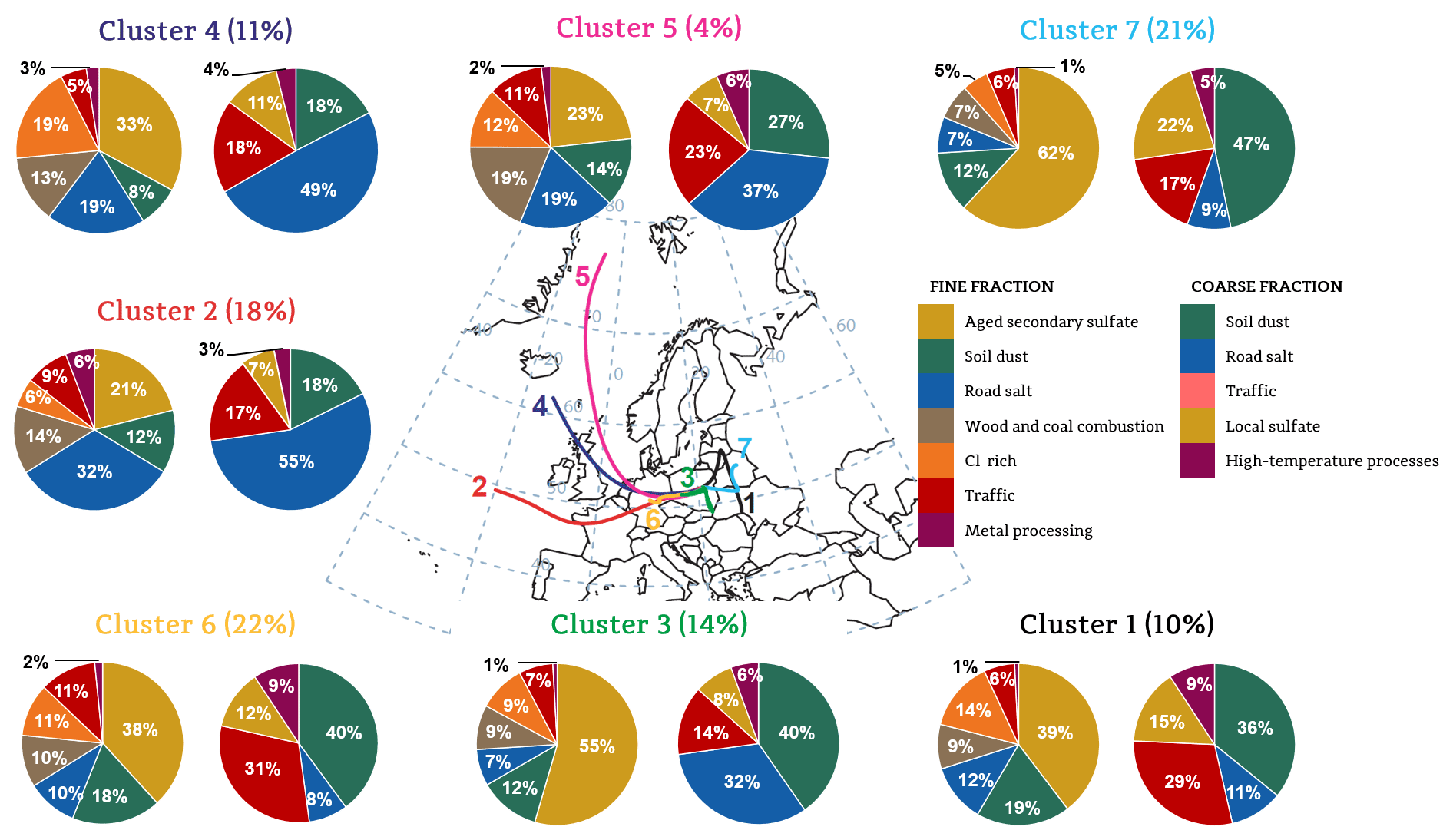
Figure 7 Trajectory cluster centroids arriving to Warsaw at 200 m (center map), with the PMF factor contribution in different clusters for the fine (left pie charts) and coarse (right pie charts) fraction. The percentage of the trajectories classified into each cluster is given in parentheses.

The most frequent advection patterns correspond to the regional slow moving air masses, which together account for 67 % of the total number of trajectories reaching the measurement site. Such flows, including short westerly trajectories (cluster 6) and trajectories recirculating over Eastern European countries (clusters 1 and 7) and over Poland (cluster 3), are characterized by the shortest trajectories (the clusters' length between 1900 and 2100 km) and the net distance traveled by an air parcel within 96 h between 550 and 850 km. Cluster 6, being the major cluster in terms of the number of trajectories (22 % of the trajectories), originates from the central part of Germany and passes further over eastern Germany, as well as over western and central Poland. The second-largest cluster in terms of the number of trajectories (21 %) is cluster 7, with its origin in eastern Belarus. The air masses pass further over the Belarus–Ukraine border and reach Warsaw from the east. A total of 10 % of the trajectories are identified in cluster 1, which start over southern Ukraine and arrive to Warsaw from the northeast, passing over Ukraine, Belarus, Latvia, and Lithuania. Cluster 3 (14 % of the trajectories) is composed of trajectories recirculating over western and southern Poland.

One-third of the trajectories correspond to fast northwesterly (clusters 4 and 5) and westerly (cluster 2) flows (Fig. 7), with the length of trajectories between 2800 and 4025 km. The air masses in clusters 2 and 4, accounting for 18 % and 11 % of the trajectories, respectively, originate from the Atlantic Ocean and pass over western European countries, while the air masses in cluster 4 are moving more from the northwesterly direction. Cluster 5, being the smallest in terms of the number of trajectories (4 %), is composed of trajectories starting from the Greenland Sea and passing over the Norwegian Sea and the North Sea. All three clusters, after crossing the central part of Germany, arrive to Warsaw from the west, passing over western and central Poland.

The analysis of the influence of the air mass origin on the PMF factor contributions shows that slow and regional flows are related to higher concentrations of the fine fraction than the coarse one, while the fast moving westerly flows show comparable levels for both fractions. In addition, regional air masses are characterized by the highest contributions of aged secondary sulfate to the fine elemental mass, accounting for 38 %, 39 %, 55 %, and 62 % for clusters 6, 1, 3, and 7, respectively. This confirms the regional transport of aged aerosol to the sampling site, in particular from the east (cluster 7) and south (cluster 3). The share of the rest of the identified sources is almost equally distributed within the clusters, pointing to a more local origin of the sources. In the case of fast Atlantic air masses, the contribution of the sources to the elemental mass is different. Clusters 4 and 5 are characterized by the highest contribution of aged secondary sulfate (33 % and 23 %, respectively), followed by road salt (19 % in both clusters), while, on the contrary, cluster 2 has the highest contribution of road salt, followed by aged secondary sulfate (32 % and 21 %, respectively). This may suggest that, although road salt is the main source of atmospheric aerosol during Atlantic flows, a partial contribution of sea spray is also highly probable. For the coarse fraction, slow regional air masses are characterized by substantially higher contributions of soil dust (36 %–47 %) than the fast westerly ones, while fast Atlantic air masses bring substantially higher loads of road salt (the shares equal 37 %–55 %). Among all clusters, metal processing and high-temperature processes have the lowest contribution to the elemental fine and coarse mass amounting to 1 %–6 % and 4 %–9 %, respectively, supporting the influence of local emission sources.

3.5 Saharan dust outbreaks

Although African dust outbreaks are more frequent in the Mediterranean basin, long-range transport of dust mainly from the Sahara desert is not unusual over Poland (e.g., Janicka et al., 2017). Such dust events were observed at the beginning (18 February) and at the end (8 March) of the measurement campaign. The back trajectory analysis shows that, during the first event, the air masses observed over Warsaw at 3000 m were advected from near-surface heights over North Africa in the warm sector of an southeastward-moving Mediterranean cyclone and rose along the warm front, while displacing northeastwards off Africa. In turn, air parcels observed at 1500 m descended from the upper troposphere behind the surface cold front of the cyclone, while also being directed northeastwards. The trajectories reaching the sampling point at 200 m a.s.l., however, came from the east (Fig. 8). The southwesterly airflows were observed for 2 d from 18 February, 01:00, until 19 February, 23:00. The advection of dust-laden airflows out of Africa toward Warsaw is evidenced by satellite imagery on 15 February (Fig. S24 in the Supplement), and both back trajectories (Fig. 8) and dust prediction models (Fig. S25 in the Supplement) indicate that they reach the study area aloft by 18 February. However, the small-scale downward movement and mixing of dust particles is not represented in the back trajectory model, and therefore, it cannot explain the dust impact at ground level. Besides, cloud coverage prevented optical remotely sensed monitoring. Therefore the presence of dust at low levels is supported primarily by the PM_2.5 chemical composition and the PMF analysis, as shown below. The operational radiosounding launched on 18 February in Legionowo (12374), around 20 km to the north of Warsaw, and surface meteorological instruments confirm the near-surface southeasterly winds in association with a high-pressure system located to the northeast of Poland, consistent with the trajectories found at 200 m a.s.l. The half-hourly wind speed at the Warsaw Okęcie Airport was over 20 km h⁻¹, only from 00:00 to 02:30, so the PM_2.5 soil contribution registered on 18 February (Fig. 9) is unlikely due to local/regional soil particulate resuspension. The radiosounding (Fig. S26 in the Supplement) shows the presence of a dry layer from near 1500 to over 2500 m a.s.l. where the wind veered to the south. This layer overlaps the top of a temperature inversion layer with the base (the atmospheric boundary layer – ABL) at 750 m a.s.l., located in a cloud top. Above the dry layer, a thick ice cloud extends above 5000 m a.s.l. The trajectories corresponding to the dry layer have a North African origin; therefore, it can be identified as a dust layer. As the dust layer overlaps the top of the inversion layer and the entrainment zone is at the base of the inversion, near the cloud top, the dust layer is located near the entrainment zone, allowing for the mixing of dust within the ABL down to the ground.

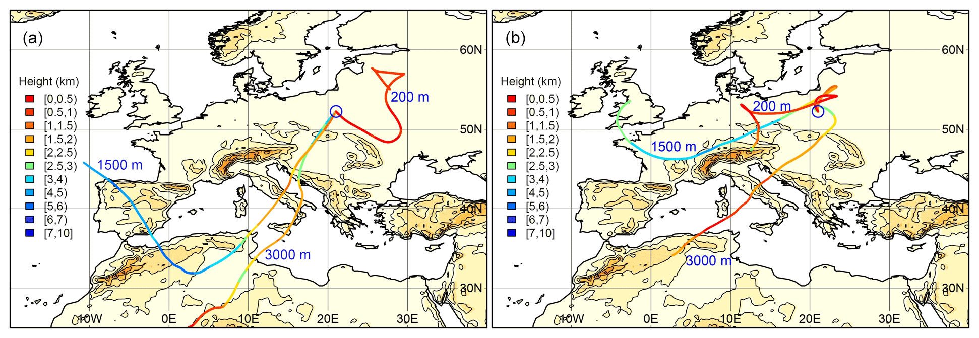
Figure 8 Air mass trajectories arriving to Warsaw at 200, 1500, and 3000 m a.s.l. at 08:00 on 18 February (a) and at 12:00 on 8 March (b). The colors along a trajectory indicate the height of the air parcels.

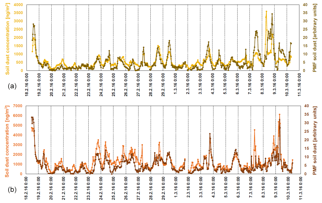
Figure 9 Hourly time series of the soil dust source contributions identified by PMF analysis (dark colors) and calculated soil component concentrations (light colors) in the fine (a) and coarse (b) fractions.

The inflow from over the Sahara desert is also evident during the second event, when the long-range transport of African dust is observed for trajectories reaching Warsaw at 3000 m (Fig. 8), after mobilization over North Africa and advection by the warm sector winds on the foreside of a cold front trailing from a developed Genoa low and primary cyclone moving in higher latitudes from the Netherlands to southern Germany.

The measurements of many elemental species allowed for the estimation of the concentrations of soil dust, which is a significant PM component. The soil dust component was calculated based on the concentrations of the oxides of the five major elements, i.e., Al, Si, Ca, Ti, and Fe, following a widely used approach given by Eq. (8) as follows (e.g., Chow et al., 2015):

$$\begin{array}{ll}{\displaystyle }\text{Soil dust}=& {\displaystyle }\mathrm{2.20}\cdot \left[\mathrm{Al}\right]+\mathrm{2.49}\cdot \left[\mathrm{Si}\right]+\mathrm{1.63}\cdot \left[\mathrm{Ca}\right]\\ \text{(8)}& {\displaystyle }& {\displaystyle }+\mathrm{1.94}\cdot \left[\mathrm{Ti}\right]+\mathrm{2.42}\cdot \left[\mathrm{Fe}\right].\end{array}$$

As can be seen in Fig. 9, strong soil dust component peaks may be observed during the days with air masses coming from Africa. In the fine fraction, the recorded peak values are as high as 2.0 and 3.5 µg m⁻³ during the first and second episode, respectively. In the coarse fraction, the concentrations of the estimated soil dust are higher with the peak levels equaling 4.7 and 6.1 µg m⁻³ during the first and second episode, respectively. In comparison, the mean concentrations of soil dust during non-episode days equaled 0.5 and 1.1 µg m⁻³ in the fine and coarse fractions, respectively. In both fractions, the time series of Soil dust sources identified by the PMF show the same peak values, and their concentrations are highly correlated with those of the calculated soil dust (r=0.75 and r=0.85 for the fine and coarse fractions, respectively), thus strengthening the attribution of these PMF factors to the soil dust.

4 Summary and conclusions

The analysis of the composition of trace elements in the fine (PM_2.5) and coarse (PM_2.5−10) fractions of particulate matter at an urban background site in central Warsaw during a high time resolution wintertime measurement campaign has been carried out for the first time in Central Europe.

The source apportionment analysis by means of three receptor models, including multivariate (PMF) and wind- (CPF) and trajectory-based (Cluster Analysis) RMs, allowed for the identification of seven factors for the fine fraction and five factors for the coarse one. Traffic-related sources (soil dust mixed with road dust, road dust, and traffic emissions) had the biggest contribution in the coarse elemental mass (together accounting for 83 %), followed by sulfates from local emissions (11.5 %). In the fine fraction, regionally transported aged secondary sulfate was found as the major source (44 %), followed by traffic-related sources (20 %). Such a high contribution of transport of secondary sulfates was also found in the daily PM_2.5 data, showing an unusual content of secondary inorganic aerosols (35 %) during the measurement campaign for the Central European urban area. The share of the remaining sources in both fractions did not exceed 15 %, with the lowest contribution of industry-related sources (metal processing and high-temperature processes) accounting for 2 % and 6 % in the fine and coarse fractions, respectively. The source polar plots based on the hourly wind data supported the identification of the possible origin areas of the different sources identified by PMF.

We can conclude that the presented findings are consistent with the previous study performed at the same urban background site (Juda-Rezler et al., 2020), which demonstrated that combustion in the residential sector within the city and in the surrounding suburban areas, followed by road transport as being the predominant sources for PM_2.5 pollution in Warsaw, using daily concentrations of PM_2.5 and its constituents, i.e., eight ions, carbonaceous matter (EC and OC), and 21 trace elements. However, the exploitation of high time resolution elemental data, despite the lack of macro components (i.e., ions and carbonaceous components), improves the source apportionment modeling results by allowing for the identification of sources that were not identified with daily time resolution, such as wood and coal combustion and the Cl-rich sources. Moreover, only the high time resolution of the concentrations of elements makes it possible to reveal and draw conclusions about the multi-faceted nature of a given element, which may have different sources in different fractions of PM. Such features were found for Cl and Cr, for which distinct temporal profiles and the correlation with different elements allowed for the identification of a diverse origin of these elements in the fine and coarse fractions. Cl was apportioned to the wintertime application of road salt for deicing purposes and a mixed source of particles rich in Cl in the coarse and fine fraction, respectively, while Cr demonstrated an industrial origin in the fine fraction and a traffic one in the coarse mode.

The applied trajectory-based receptor modeling based on the high time resolution enables following the transport pathways of the aerosols. Our results showed a substantial contribution of regionally transported aged aerosols, in particular from the south and east of Warsaw, while a more local impact of the rest of the identified sources was found. Thus, both emission control measures in the upwind areas, as well as the control of local emissions (mainly in residential combustion and traffic- and industry-related sectors) should be applied in the city for effective air pollution control in winter.

The analyses carried out in this study allowed also for identification of two intense Saharan dust outbreaks in Warsaw. During these episodes, long-range transport of dust from the Sahara desert was observed for trajectories arriving at 1500 and 3000 m. The calculated concentrations of soil dust showed a strong impact in both fractions – the levels of the soil component during the Saharan episodes were 7 and 6 times higher than the mean concentrations observed during non-episodes days in the fine and coarse fractions, respectively.