Wildfire smoke-plume rise: a simple energy balance parameterization

The buoyant rise and the resultant vertical distribution of wildfire smoke in the atmosphere have a strong influence on downwind pollutant concentrations at the surface. The amount of smoke injected vs. height is a key input into chemical transport models and smoke modelling frameworks. Due to scarcity of model evaluation data as well as the inherent complexity of wildfire plume dynamics, smoke injection height predictions have large uncertainties. In this work we use the coupled fire–atmosphere model WRF-SFIRE configured in large-eddy simulation (LES) mode to develop a synthetic plume dataset. Using this numerical data, we demonstrate that crosswind integrated smoke injection height for a fire of arbitrary shape and intensity can be modelled with a simple energy balance. We introduce two forms of updraft velocity scales that exhibit a linear dimensionless relationship with the plume vertical penetration distance through daytime convective boundary layers. Lastly, we use LES and prescribed burn data to constrain and evaluate the model. Our results suggest that the proposed simple parameterization of mean plume rise as a function of vertical velocity scale offers reasonable accuracy (30 m errors) at little computational cost.

1 Introduction

Predictions of surface concentrations of wildfire smoke by regional and global chemical transport models depend on the initial equilibrium height of the smoke plume. Plume rise, which determines this equilibrium height, is widely recognized as an area of uncertainty (Goodrick et al., 2013; Paugam et al., 2016). Traditionally, many operational smoke modelling frameworks relied on plume rise equations originally developed by Briggs (1975) for industrial smokestacks (Larkin et al., 2010; Pavlovic et al., 2016). Yet several studies suggest that this approach may not be appropriate for wildfires (Pavlovic et al., 2016; Heilman et al., 2014; Freitas et al., 2007).

In a recent review of existing plume rise parameterizations, Paugam et al. (2016) highlight three notable models that stand out in the literature: those by Freitas et al. (2007), Sofiev et al. (2012) and Rio et al. (2010). Both Freitas' and Rio's approaches use first principles to characterize plume temperature, vertical velocity and entrainment. While the approach by Freitas et al. (2007) provides prognostic 1-D equations that can be solved as a stand-alone “offline” model, the approach by Rio et al. (2010) is implemented as a sub-grid effect within a host chemistry transport model. Notably, both consider an idealized heat source to represent the fire. To initialize the plume at the lower boundary, simplified fire geometry (circular and rectangular for Freitas' and Rio's models, respectively) with a uniform heat flux is assumed. Sofiev's semi-empirical approach relies on energy balance and dimensional analysis while using satellite data to both initialize and constrain the parameterization. Unlike Briggs' equations, all of the above models address wildfire plumes specifically, yet much research is needed to reduce the large uncertainties associated with the model predictions (Mallia et al., 2018). Moreover, it is unclear whether unreliable predictions should be attributed to the fire input parameters or the plume rise model itself.

One of the central challenges in plume rise model development has been the scarcity of comprehensive model evaluation data (Coen et al., 2012b; Ottmar et al., 2016). To date, information on wildfire smoke emissions and dispersion has largely been derived from two distinct sources: remotely sensed data and prescribed burn campaigns. While increasing numbers of satellite observations contribute to a more complete plume climatology (Val Martin et al., 2010), the data are subject to biases and lack direct spatiotemporal links to fire behaviour (Ichoku et al., 2012). In contrast, field campaigns, such as Prescribed Fire Combustion and Atmospheric Dynamics Research Experiment (RxCADRE) (Ottmar et al., 2016) and the Fire and Smoke Model Evaluation Experiment (FASMEE) (Prichard et al., 2019), provide the necessary level of detail for model validation studies. However, such datasets typically capture a modest range of fire and atmospheric conditions.

Our approach, therefore, is to develop a synthetic plume dataset that addresses the limitations of the available observational data. As the vast majority of smoke plumes remain in or just above the atmospheric boundary layer (ABL) (Val Martin et al., 2010; Mallia et al., 2018), we use large-eddy simulations (LESs) to focus on local-scale and mesoscale plume dynamics. Using a coupled model, we simulate a wide range of fire and atmospheric conditions (Sect. 2). Based on this synthetic LES data (hereafter referred to as “data”), we propose a simple energy balance model for predicting plume rise of crosswind integrated (CWI) smoke from a non-uniform fireline (Sect. 3). We use the synthetic plume dataset to constrain and evaluate our plume rise parameterization. We then demonstrate, with both numerical and prescribed burn data, that within the range of tested conditions this parameterization offers high speed and accuracy (Sect. 4). Moreover, it provides the means for classifying penetrative vs. non-penetrative plumes, which is key for subsequent dispersion modelling (Sofiev et al., 2012; Val Martin et al., 2012).

The proposed approach is geared toward regional smoke modelling frameworks (e.g. BlueSky and BlueSky Canada). Government agencies, air quality managers and fire response teams depend on these operational tools and their accuracy to issue air quality warnings, evacuation orders and to help mitigate human health impacts. Yet, model evaluation studies suggest that plume rise estimation remains a weak link within smoke modelling systems (Raffuse et al., 2012; Val Martin et al., 2012; Chen et al., 2019). Moreover, existing methods struggle to reliably identify which plumes remain in the ABL and which penetrate it. Therefore, the broad goal of the work is to address some of these challenges and improve the accuracy of plume rise predictions for regional air quality applications.

2 Development of a synthetic plume dataset

We devise a synthetic plume dataset using a coupled fire–atmosphere model WRF-SFIRE, which combines the well-established Weather Research and Forecasting (WRF) model with a semi-empirical fire spread algorithm called SFIRE (Mandel et al., 2014; Mallia et al., 2020; Coen et al., 2012a; Kochanski et al., 2013; Clements et al., 2006; Kochanski et al., 2019). The model allows one to explicitly resolve plume dynamics while parameterizing fuel combustion. One of the primary advantages of using WRF-SFIRE is that it supports two-way coupling between the atmosphere and the fire behaviour model, allowing it to capture some of the complex dynamical feedbacks that exist between the fire and the atmosphere (Prichard et al., 2019). Heat and moisture fluxes from the simulated burn provide forcing to the atmosphere, affecting local wind flow and thermodynamics. This in turn influences the modelled fire behaviour. The following sections detail the numerical setup of WRF-SFIRE and the scope of the dataset, as well as our approach to defining “ground truth” for model evaluation.

2.1 Numerical configuration

WRF-SFIRE was configured in idealized large-eddy resolving mode. Much of our numerical setup was adopted from a case study of a real prescribed burn as detailed in Moisseeva and Stull (2019), to ensure the simulations represent physical conditions backed by model evaluation. Due to high computational demands of LES runs, we focused on the local-scale and mesoscale, considering only the initial buoyant plume rise of smoke in typical daytime atmospheres. Key parameters varied were ambient wind, fuel category, vertical potential-temperature profile and fireline length, denoted as conditions W, F, R and L, respectively (detailed further in Sect. 2.2).

Each 10 km×20 km domain with 40 m horizontal grid spacing was initialized with uniform ambient westerly wind W and vertical temperature profile R. Depending on the sounding R, the simulations were performed in either a shallow (3000 m) or a deep (5000 m) domain, with 51 or 71 hyperbolically stretched vertical levels, respectively. A constant, uniform lower-boundary surface thermal flux (tke_heat_flux) in the ambient environment and lateral periodic boundary conditions were imposed to produce a turbulent well-mixed layer. We used full surface initialization (sfc_full_init =.true.), with the lower boundary characteristics set to USGS (United States Geological Survey) values for land use most closely matching the Anderson fuel category F (Anderson, 1982). The corresponding surface roughness lengths added various levels of wind shear to each domain to produce a more realistic non-uniform vertical wind profile during spin-up of the environment before the fire was initialized in the LES.

Initial convection in the ambient environment was triggered using a perturbed surface temperature field. On average, a near-stationary turbulence spectrum was achieved within the first 30 min of run start. The “restart” file generated at the end of 1 h of spin-up was used to initialize the main burn simulation, ensuring the fire was ignited in a well-mixed turbulent ABL.

The fire was initialized over a 1 min interval using a straight line of length L. The ignition line was placed 1 km downwind of the western edge of the domain and centered in the north–south direction (sample illustration of this setup can be found in Appendix A). With a refinement ratio of 10 in each horizontal direction, the fire was simulated on a 4 m sub-grid mesh.

The “smoke plume” was modelled with a passive tracer emitted proportionally to the mass and type of fuel burned. The rate of release was controlled by an assigned emission factor representing PM_2.5 for each fuel category, based on values provided by Prichard et al. (2017) (see namelist.fire_emissions in the Supplement).

A summary of key configuration details can be found in Table 1, as well as in sample namelist initialization files provided in the Supplement.

2.2 Test conditions

Table 2 summarizes the key parameters that were varied to produce the synthetic dataset. The reason for considering the given conditions is twofold: these parameters (i) have been widely acknowledged as having a strong impact on plume behaviour and (ii) can be obtained (and provided as input for the parameterization) under real-world scenarios.

The range of ambient winds tested was bound largely by numerical constraints. Due to cyclic boundary conditions, wind speeds higher than 12 m s⁻¹ would require a much larger domain to prevent smoke recirculation. For the lower bound on our wind condition W, we needed to ensure that sufficient wind speed was maintained to propagate the fire. The spread algorithm used within the LES applies a correction factor under low-wind-speed conditions to prevent the fire from extinguishing itself. While necessary for numerical reasons, this effect is not physical, so winds below 3 m s⁻¹ were excluded from our dataset.

We used nine different atmospheric profiles (R condition) to initialize the model. We varied the following features for each initialization:

• initial ABL height (500–1600 m)

• potential-temperature lapse rate above inversion (0–20 K km⁻¹)

• initial ABL temperature (290–300 K).

Following spin-up (Sect. 2.1) under variable winds and surface conditions, this produced nine sets of soundings, shown in Fig. 1 with ABL depths of approximately 600–2000 m.

Mandel, 2020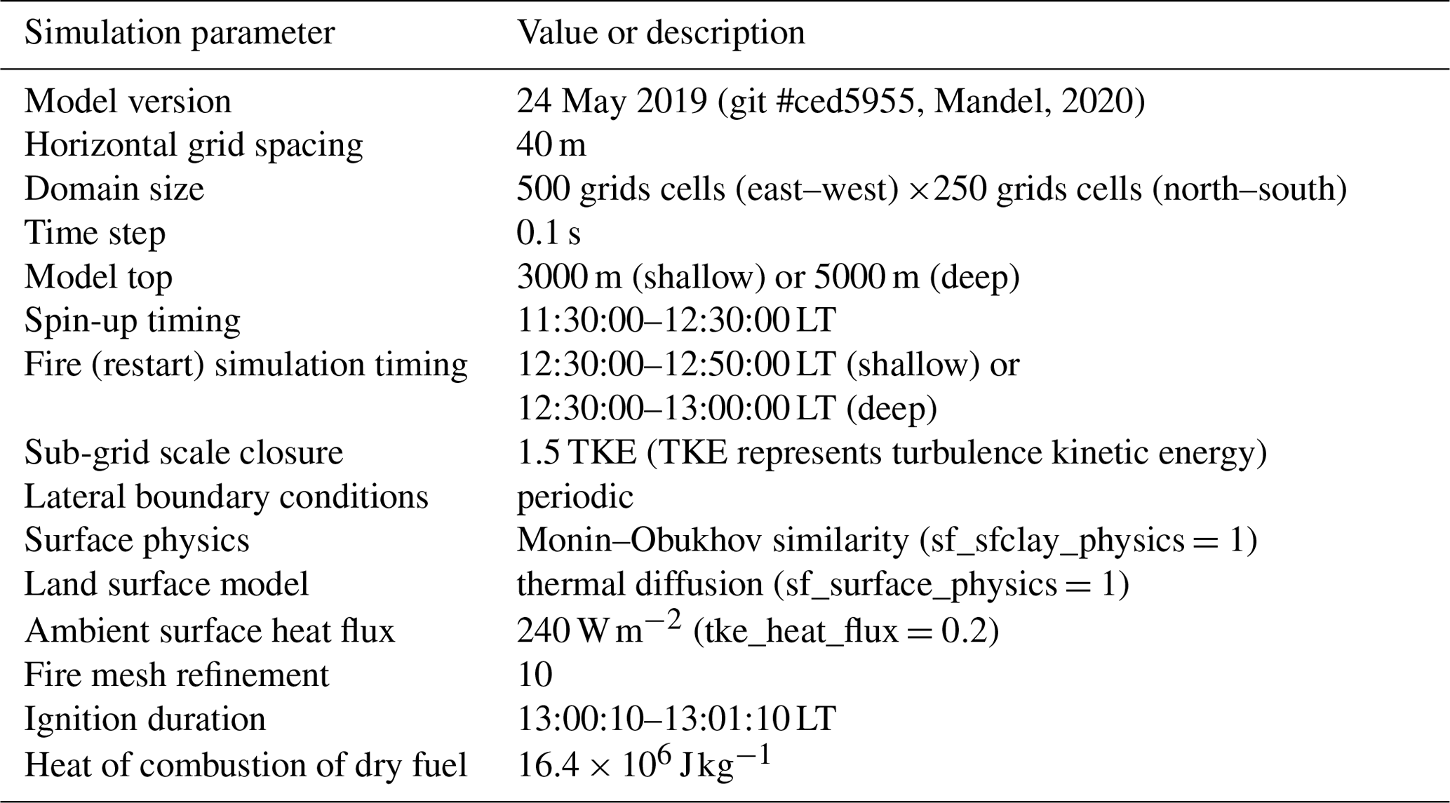

Table 1 Key parameters of numerical domain setup.

Table 2 Test conditions included in the synthetic plume dataset. The count indicates the number of unique values used within the specified range.

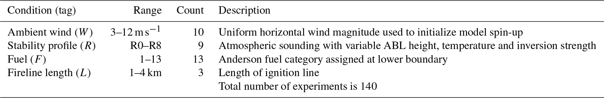
Figure 1 Pre-ignition potential-temperature profiles (stability condition R). Colors correspond to initial soundings used for model spin-up.

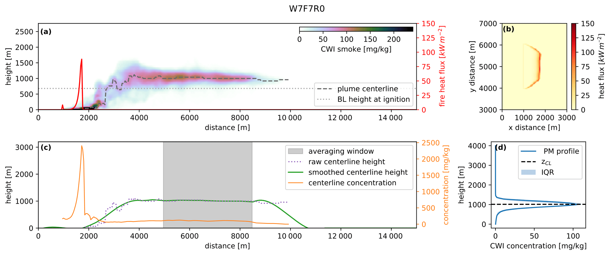
Figure 2 Illustration of the approach to identifying a quasi-stationary downwind region in CWI smoke distribution using a sample LES experiment. (a) CWI smoke concentrations. Also shown are plume centerline height (dashed), z_i (dotted) and CWI fireline intensity (solid red, secondary axis). (b) Plan view of fire heat flux showing the fireline. (c) Quasi-stationary region (grey shading). Also shown are raw (dotted purple) and smoothed (solid green) centerline heights and the tracer concentration gradient (solid orange, secondary axis). (d) Representative downwind smoke distribution. The profile (solid blue line) is obtained by horizontally averaging the CWI smoke concentrations in the quasi-stationary region (dashed grey in c). Also shown are the IQR (interquartile range, light blue shading) and the derived smoke injection centerline height z_CL (dashed black).

We tested all fuel categories available within the model (F condition), and we varied the length of the fireline (L condition) between 1 and 4 km. Weakly buoyant non-penetrative plumes whose smoke remained within the well-mixed ABL were excluded from the dataset, as their behaviour is governed by different physics. A tabulated summary of all combinations included can be found in Appendix B.

Note that varying a single condition while holding the rest constant does not result in a controlled experiment isolating its impact on plume rise. Because WRF-SFIRE incorporates fire–atmosphere coupling, the problem is not well constrained. For example, by varying fuel type F alone while holding the rest of the test conditions constant, we obtain a set of fires with diverse shapes, sizes, intensities, fireline depths, rates of spread and heat release. This reflects the complexity of non-linear interactions that exist between the fire and the atmosphere. As a result, the parameter space captured within our LES dataset is much greater then the four conditions described in Table 2.

2.3 Defining smoke injection height

Given non-stationary fire and atmospheric conditions, determining a consistent definition of an equilibrium smoke injection height is not a trivial task. It requires separating buoyant rise from dispersion while excluding the effects of initial momentum overshoot and accounting for the advection due to varying ambient and fire-generated winds.

A common way of examining vertical distributions of pollutants in the context of air quality is to consider CWI concentrations. This allows one to reduce the problem to two dimensions, with the plume centerline being defined simply as the CWI concentration maximum at each location downwind of the source. Theoretically, under stationary conditions there exists an equilibrium height around which the centerline eventually oscillates. In reality, as well as in our LES experiments, neither the ambient nor the fire conditions are stationary. The changing location, shape, and intensity of the fire and the ABL warming and growth, as well as the development of fire-coupled winds and vorticity, continually modify the conditions.

As a result, our approach is based on defining a region where the concentration distribution is quasi-stationary. We consider the last frame of each simulation for this analysis. Using CWI tracer values, we locate the plume centerline (Fig. 2a). Due to random effects of ABL thermals, as well as fluctuations in fire intensity and propagation speed, both centerline height and concentration can vary near the heat source. These oscillations are naturally suppressed in the stable layers above the ABL, as the plume travels downwind and undergoes additional widening and mixing. To obtain the quasi-stationary region for each individual plume, we first calculate the change in tracer concentration along the centerline. We then use a smoothing function to reduce the effect of random turbulent oscillations in both the centerline height and the tracer concentration gradient along the centerline. The downwind region where both of these parameters are not changing rapidly are then considered quasi-stationary. Additional details of this filtering method are provided in Appendix C.

The vertical CWI distribution of tracers is then averaged in the downwind direction over the identified quasi-stationary regions (shaded in grey in Fig. 2c) to produce a representative downwind distribution for each plume (Fig. 2d). We define the “true” injection height z_CL as the mean height of smoothed centerline over the averaging region. The resultant dataset of z_CL values is used to constrain and evaluate the proposed smoke injection height parameterization introduced in the following sections.

3 Smoke injection height model for penetrative wildfire plumes

A common approach to predicting the final equilibrium centerline height of wildfire smoke is to first estimate the initial buoyant energy of the hot rising smoke (Briggs, 1975; Sofiev et al., 2012; Anderson et al., 2011). After the smoke plume entrains surrounding ABL environmental air and cools, the remaining energy is spent doing work to push the cooled smoke plume up into the statically stable capping inversion.

The relationship between final and initial energies is often rewritten to show that the potential energy per unit mass (PE) of smoke penetration equals some fraction c₁ of initial heat released from the fire. In kinematic units, the initial heat input has units similar to a kinetic energy per unit mass (KE). The empirical parameter c₁ is usually estimated based on concepts of entrainment into the rising smoke plume (Cushman-Roisin, 2014).

$$\begin{array}{}\text{(1)}& {\displaystyle }{\displaystyle }\text{PE}=c_{\mathrm{1}}\text{KE}\end{array}$$

The PE of smoke-plume penetration into the capping inversion can be written as

$$\begin{array}{}\text{(2)}& {\displaystyle }{\displaystyle }\text{PE}=g^{\prime }{z}^{\prime },\end{array}$$

where the penetration distance z^′ of the final equilibrium smoke centerline z_CL above reference height z_s (near the top of the well-mixed portion of ABL) is

$$\begin{array}{}\text{(3)}& {\displaystyle }{\displaystyle }{z}^{\prime }=z_{\text{CL}}-z_s.\end{array}$$

The static-stability variable g^′ for the plume-penetration region is

$$\begin{array}{}\text{(4)}& {\displaystyle }{\displaystyle }{g}^{\prime }=g{\displaystyle \frac{{\mathit{\theta }}_{\text{CL}}-{\mathit{\theta }}_s}{{\mathit{\theta }}_s}}=g{\displaystyle \frac{{\mathit{\theta }}^{\prime }}{{\mathit{\theta }}_s}},\end{array}$$

where θ_CL and θ_s are the potential temperatures of the ambient environment at z_CL and z_s, respectively, and ${\mathit{\theta }}_{\text{CL}}-{\mathit{\theta }}_s={\mathit{\theta }}^{\prime }$.

The KE can be estimated using a velocity scale w_f as

$$\begin{array}{}\text{(5)}& {\displaystyle }{\displaystyle }\text{KE}=\mathrm{0.5}{w}_f^{\mathrm{2}}.\end{array}$$

Traditionally, the bulk potential-temperature difference across the smoke-plume penetration region θ^′ is expected to be relevant for only the PE portion of Eq. (1). However, we found from the LES runs for a wide range of fire and environment conditions that the KE also depends on the same potential-temperature difference. This dependence can be expressed in the velocity scale:

$$\begin{array}{}\text{(6)}& {\displaystyle }{\displaystyle }{w}_f={\displaystyle \frac{I}{z_i{\mathit{\theta }}^{\prime }}}.\end{array}$$

This velocity scale is related to the fireline intensity parameter I, which is the kinematic heat flux into the atmosphere integrated across the fireline depth (in units of K m² s⁻¹), and to the mixed-layer depth z_i. Note that I effectively corresponds to the kinematic form of Byram's fireline intensity (in units of kW m⁻¹).

We speculate that this interesting result is because smoke from a fire does not rise through a passive environment, as is often assumed for Briggs types of plume entrainment models. Instead, the fire and the environment interact in many complex ways. Some of these include vertical-to-bent-over vortices on the ends of the fireline that rapidly mix environmental air into the buoyant smoke plume, modulation of fire intensity and fire updrafts by translation of ambient thermals across the fireline, plumes of enhanced convergence and updraft along the fireline, mass conservation as descending air beneath the extended smoke plume lowers the local mixed-layer depth, and other factors.

Thus, Eq. (1) becomes

$$\begin{array}{}\text{(7)}& {\displaystyle }{\displaystyle }{g}^{\prime }{z}^{\prime }=c_{\mathrm{2}}{\left[{\displaystyle \frac{I}{z_i{\mathit{\theta }}^{\prime }}}\right]}^{\mathrm{2}},\end{array}$$

where c₂=0.5c₁.

The above equation can be rearranged into the following form:

$$\begin{array}{}\text{(8)}& {\displaystyle }{\displaystyle }{z}_{\text{CL}}-z_s=C{\left[{\displaystyle \frac{g\left({\mathit{\theta }}_{\text{CL}}-{\mathit{\theta }}_s\right)}{{\mathit{\theta }}_s\left(z_{\text{CL}}-z_s\right)}}\right]}^{-\frac{\mathrm{1}}{\mathrm{2}}}{\left\{{\displaystyle \frac{gI\left(z_{\text{CL}}-z_s\right)}{{\mathit{\theta }}_s{z}_i}}\right\}}^{\frac{\mathrm{1}}{\mathrm{3}}},\end{array}$$

where the dimensionless empirical parameter is C≈1. The factors in square and curly brackets with their corresponding powers have units of time and velocity, respectively. This relationship is plotted in Fig. 3. It provides quite an acceptable fit to the data over a wide range of 140 combinations of fire and atmospheric conditions simulated.

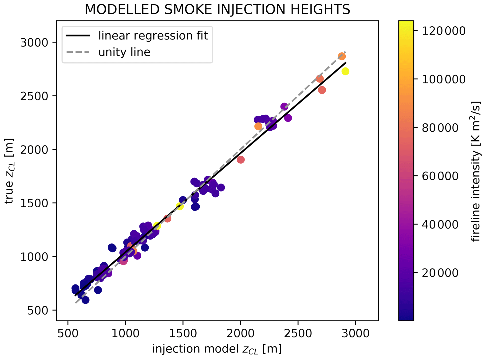
Figure 3 Comparison of true (as shown in Fig. 2) and modelled (from Eq. 8) smoke injection heights. Scatter points represent the 140 individual plume experiments within the LES dataset, with colors corresponding to fireline intensity I. The solid black line and dashed grey line denote the linear regression fit and unity line, respectively.

Equation (8) suggests that the relevant length and temperature scales ($z^{\prime },{\mathit{\theta }}^{\prime }$) depend not on the capping inversion strength alone (or on the tropospheric lapse rate above the capping inversion alone) but on the bulk potential-temperature differences across the smoke-plume penetration region, z_CL−z_s. Equation (8) is implicit in that the desired plume centerline equilibrium height z_CL appears in both the left and right sides of the equation. The plume centerline height also defines where θ_CL is retrieved from the atmospheric sounding; namely, z_CL is implicit in both Eqs. (7) and (8). However, for any specific fire and environment conditions, values of z_CL are easily found by iteration (see Appendix E). Steps for estimating input parameters required for the proposed injection model from the LES data are summarized in Appendix D.

Alternatively, for a small sacrifice in accuracy, we can obtain an explicit solution by considering an idealized version of the atmospheric profile, consisting of an adiabatic mixed layer, entrainment zone and a stable uniformly stratified free atmosphere above (Fig. 4). In such a case γ is defined as the overall potential-temperature gradient of the free atmosphere and z_s as the height corresponding to the intercept of γ and the well-mixed portion of the ABL profile. Then, using Eq. (8), z_CL can be found explicitly as

$$\begin{array}{}\text{(9)}& {\displaystyle }{\displaystyle }{z}_{\text{CL}}=C^{\frac{\mathrm{3}}{\mathrm{2}}}{\left[{\displaystyle \frac{{\mathit{\theta }}_s}{g}}\right]}^{\frac{\mathrm{1}}{\mathrm{4}}}{\left[{\displaystyle \frac{I}{z_i}}\right]}^{\frac{\mathrm{1}}{\mathrm{2}}}{\left[{\displaystyle \frac{\mathrm{1}}{\mathit{\gamma }}}\right]}^{\frac{\mathrm{3}}{\mathrm{4}}}+z_s.\end{array}$$

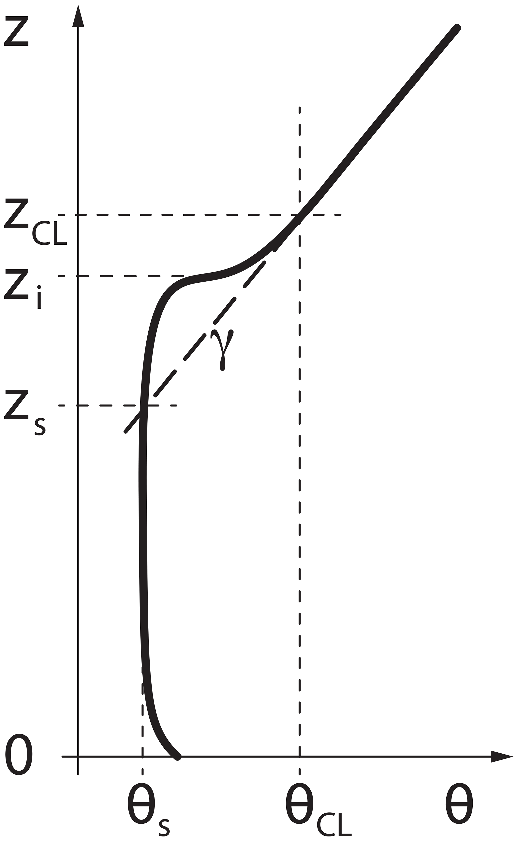
Figure 4 Idealized potential-temperature profile θ vs. height with constant stable-layer lapse rate γ.

4 Results

To assess the accuracy of the proposed smoke injection height parameterization (Eq. 8), we performed two sets of verification studies. The first approach is based on using the synthetic plume dataset to perform model evaluation, bias correction and sensitivity analysis with idealized data. The second portion of this section applies our approach to a case study of a real prescribed burn (RxCADRE 2012).

4.1 Numerical results

Shown in Fig. 3 are true and parameterized smoke injection heights. The former is obtained directly from the LES, as per Sect. 2.3. The latter is determined iteratively using the proposed smoke injection height parameterization (see Appendix E for implementation details).

Individual prediction errors do not appear to be a function of fireline intensity, as indicated by scatter point color in Fig. 3, or ambient winds (not shown). While, overall, the model performance is encouraging, the small discrepancy between the unity and regression lines suggests a linear bias. This can be remedied by applying bias correction using regression parameters from the fit shown in Fig. 3. This optimized model produces errors on the order of 20–30 m, as suggested by the interquartile range shown in Fig. 5d. Model bias will be addressed in further detail in Sect. 5.

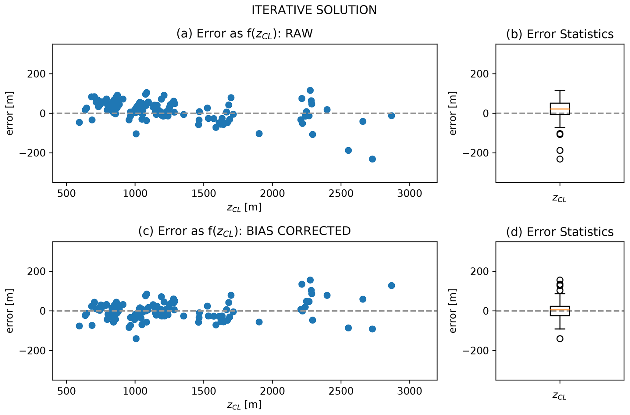
Figure 5 Performance of the smoke injection height parameterization based on the iterative solution (Eq. 8). (a) Non-bias-corrected model prediction error (true – modelled z_CL) as a function of z_CL. (b) Error statistics for the non-bias-corrected model. The box and whiskers span the interquartile range (IQR) and 1.5× IQR, respectively. Median value is shown in orange. (c) Bias-corrected model prediction error as a function of z_CL. (d) Error statistics for bias-corrected model.

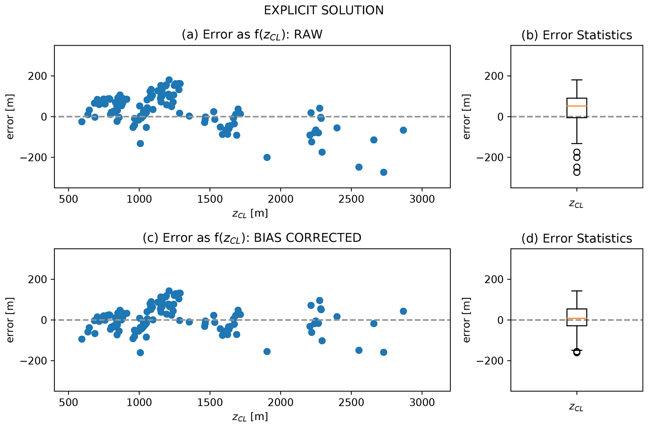
Figure 6 Performance of the smoke injection height parameterization based on the explicit solution (Eq. 9). (a) Non-bias-corrected model prediction error (true – modelled z_CL) as a function of z_CL. (b) Error statistics for the non-bias-corrected model. The box and whiskers span interquartile range (IQR) and 1.5× IQR, respectively. Median value is shown in orange. (c) Bias-corrected model prediction error as a function of z_CL. (d) Error statistics for bias-corrected model.

Given smooth averaged profiles from the synthetic dataset and excluding condition R8 (adiabatic free atmosphere), the explicit solution using Eq. (9) offers comparable accuracy to the iterative version for both raw and bias-corrected datasets (Fig. 6). We address the limitations of using the explicit approach in Sect. 5.5.

4.2 Model sensitivity

To assess how sensitive the smoke injection model performance is to the particular choice of bias correction parameters, we partition our original plume dataset into training and testing groups through random sampling. We obtain the linear bias correction parameters using training data only (80 % of runs). We then apply our bias-corrected iterative solution to the test group (remaining 20 % of the runs) and assess model accuracy. Figure 7 summarizes model performance and sensitivity, based on 10 trials of sampling with replacement. Consistently high Pearson correlation values shown in the trial histogram in Fig. 7c are encouraging and suggest that the particular choice of simulations used in bias correction does not have a strong impact on model accuracy.

Figure 7 Analysis of model sensitivity to the choice of bias correction parameters. (a) Error distributions for individual trials using independent (test) data. (b) Error distribution for all trials using independent (test) data. (c) Sensitivity of R value (correlation coefficient) for all trials.

4.3 Evaluation with observations

Next, we apply the proposed model to a real-life case study. We use observational data from the RxCADRE L2G prescribed burn (Ottmar et al., 2016) and its numerical simulation (Moisseeva and Stull, 2019). This case study was selected based on (i) the comprehensive nature of the observational dataset, (ii) the penetration of the plume above ABL top and (iii) the availability of a completed model validation study, confirming that WRF-SFIRE reasonably captures the smoke plume produced during the burn.

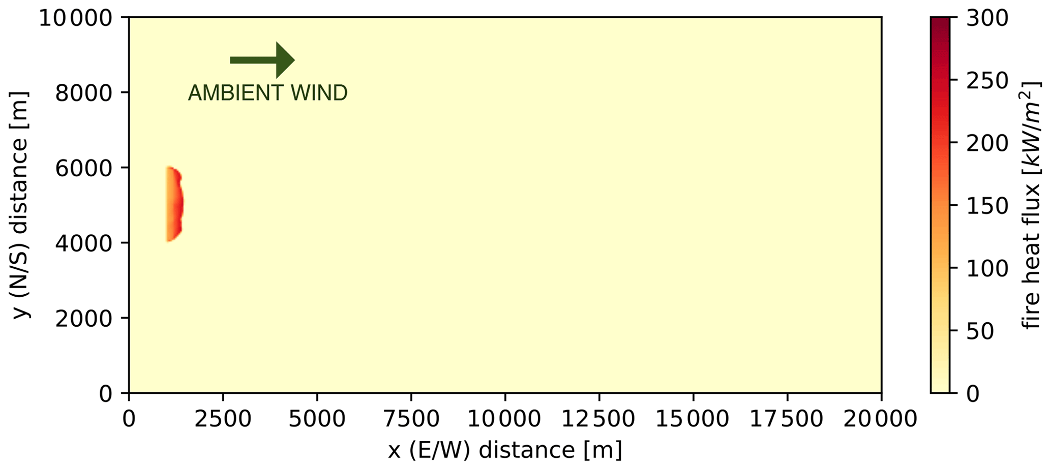
Shown in Fig. 8 is the strip headfire pattern used to ignite the grass plot. We estimate the burn's input fireline intensity parameter I in two different ways: from raw data collected during the burn and from the numerical simulation.

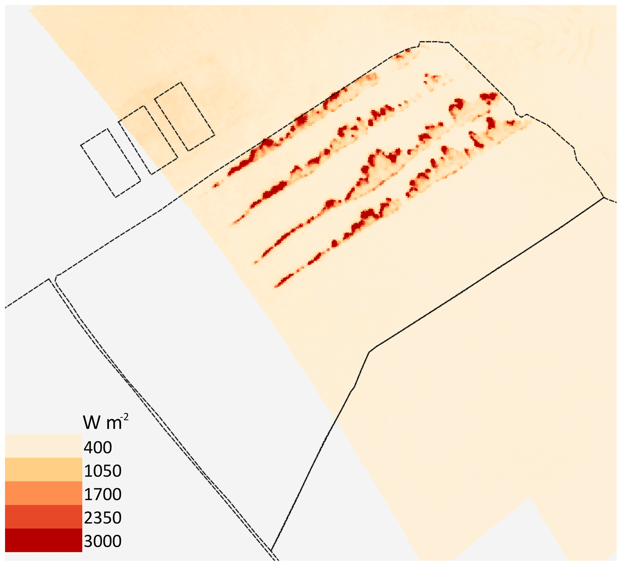
Figure 8 Long-wave infra-red (LWIR) image of L2G lot during ignition (12:32:02 CST) with dashed black lines denoting burn perimeters.

The observation-based value I_obs is derived from the integral heat flux data obtained from the Highly Instrumented Plots (HIPs) fire behaviour package (FBP) sensors (Jimenez and Butler, 2016). We use the provided time-integrated values, averaging between all sensors with confirmed fire at the sensor location (as indicated by video footage Butler et al., 2016). We then obtain the mean value (in kinematic units) of 236 K m s⁻² and multiply it by the average measured rate of spread (ROS) of 0.38 m s⁻¹ (Butler et al., 2016) for the same sensors to convert to spatially integrated heat flux for a single fireline. We assume that this value is representative of the remaining three firelines; hence,

$$\begin{array}{}\text{(10)}& {\displaystyle }{\displaystyle }{I}_{\text{obs}}=\mathrm{236}\cdot \mathrm{0.38}\cdot \mathrm{4}=\mathrm{359}\end{array}$$

(in units of K m² s⁻¹). Note that raw data for both heat fluxes and ROS values have extremely large associated uncertainties. Observed ROS values vary by nearly a factor of 2, depending on the measurement technique used. While we have included only locations with ignition confirmed by video footage in our calculations, heat fluxes still vary up to a factor of 4 between sensors.

For comparison, we also obtain an LES-based integrated fireline intensity value I_LES. Due to wind shear, as measured by the sounding launched prior to the burn (10:00:00 CST), the CWI direction at the surface differs from the one used to estimate CWI smoke. Hence, I_LES was estimated by assuming 125^∘ rotation of LES fields, based on the lowest available wind direction measurement. We use the trapezoidal rule to numerically integrate the mean crosswind heat flux along the depth of the fireline (see Appendix D) and find I_LES=1002 K m² s⁻¹.

We apply our iterative solution (Eq. 8) to find two z_CL estimates based on I_obs and I_LES, and we compare them to the CWI smoke injection height obtained from the LES. The results are shown in Fig. 9. The parameterized injection heights are underpredicted by 20 and 70 m for LES- and observation-derived I values, respectively.

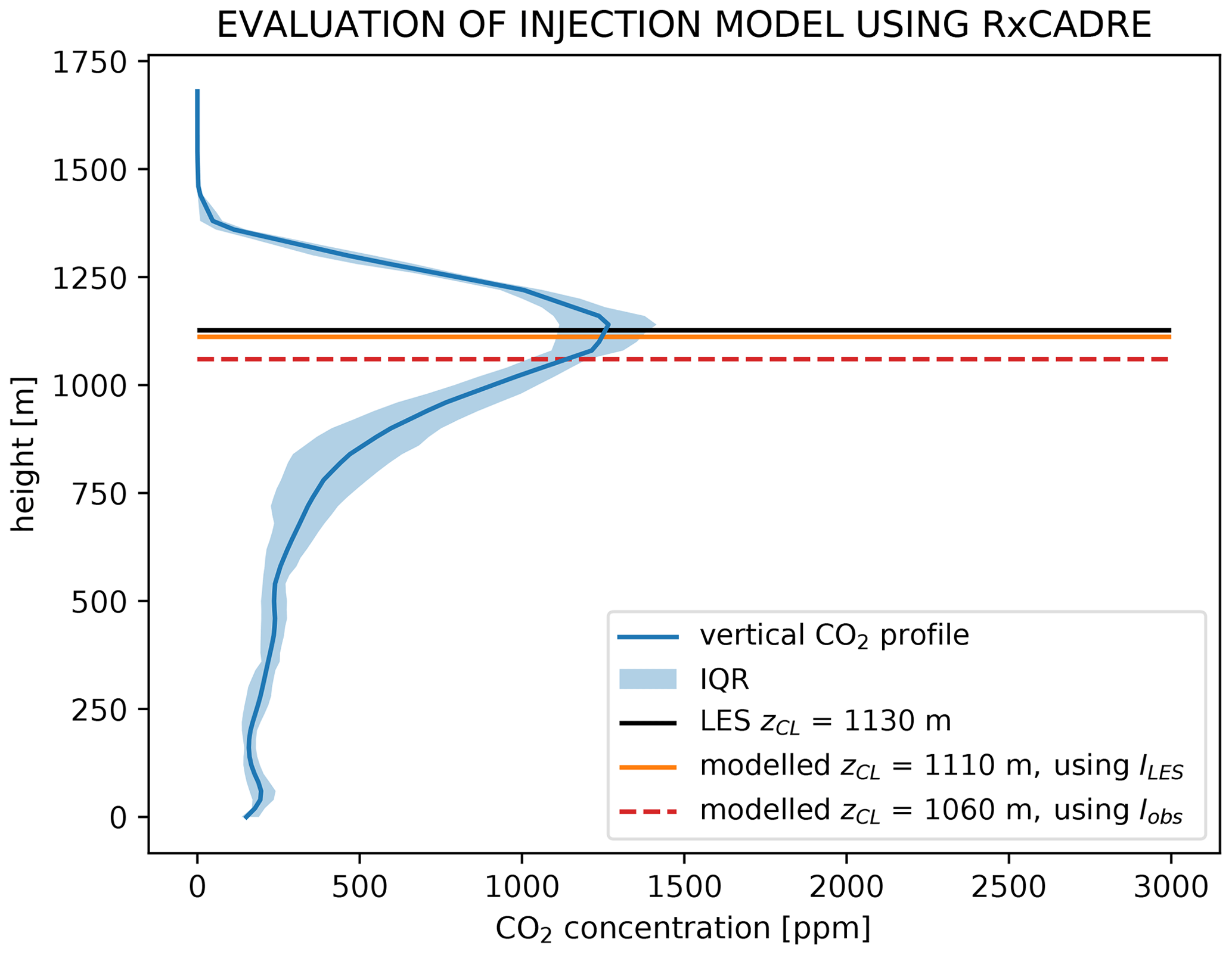
Figure 9 Model evaluation using a case study of a real prescribed burn (RxCADRE 2012). CWI smoke concentration profile shown in blue. True z_CL obtained directly from LES shown in solid black. Solid orange and dashed red lines correspond to z_CL estimates obtained using the iterative solution of the proposed smoke injection height parameterization (Eq. 8), based on LES- and observation-derived fireline intensities, respectively.

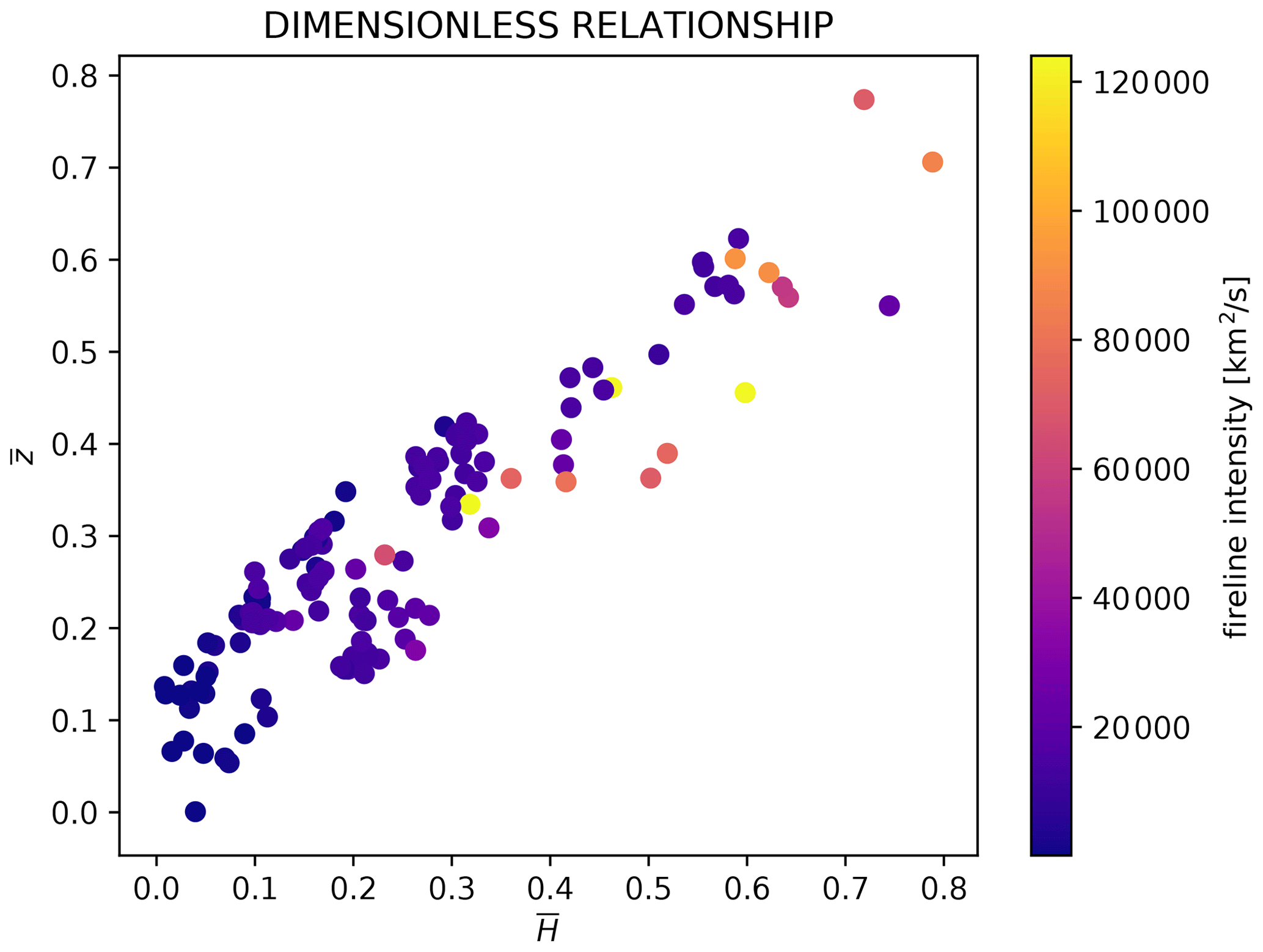
Figure 10 Similarity solution for dimensionless groups $\stackrel{\mathrm{‾}}{H}$ and $\stackrel{\mathrm{‾}}{z}$, corresponding to the right-hand side (RHS) and left-hand side (LHS) of Eq. (13), respectively. Scatter points represent individual LES runs, colored by fireline intensity parameter I.

Table 3 Identifying non-penetrative plumes using visual analysis vs. automated classification. Plume name denotes wind condition W, fuel type F and initial atmospheric profile R.

5 Discussion

5.1 Plume classification

In previous sections we apply an energy balance parameterization to predict the mean smoke injection height z_CL of a given penetrative plume. For this purpose, only plumes rising above ABL top z_i were included in the synthetic plume dataset used to constrain and evaluate the approach (see Table B1). In this section, we step back and consider all performed simulations, to determine whether the same equations can also be used to classify penetrative vs. non-penetrative plumes.

The synthetic dataset described in Sect. 2.2 consisted of 140 runs and excluded seven simulations, where the plume remained trapped in the ABL (see Tables B1 and 3). We determined this by visual analysis of CWI centerline and smoke fields. The excluded plumes typically exhibited oscillatory or irregular centerline behaviour (within the ABL, such as shown in the example in Fig. B1) with little or no smoke injected above z_i. For several combinations of fire and atmospheric conditions, however, making the distinction was challenging. For this reason, we included these “marginally penetrative” plumes in the dataset.

In real-world applications, classification is a fundamental first step in plume rise parameterization processes (Sofiev et al., 2012). A viable automated method for categorizing penetrative vs. non-penetrative plumes requires that the distinction be made based on available input parameters rather than smoke observations (as they are typically not available at the time of making a forecast).

Conveniently, we can use Eq. (8) to obtain a z_CL estimate for any combination of input parameters without prior knowledge of plume type. Hence, it can be applied as a classifier by requiring that for a penetrative plume

$$\begin{array}{}\text{(11)}& {\displaystyle }{\displaystyle }{z}_{\text{CL}}>z_{i+},\end{array}$$

where z_i+ denotes the height of the upper edge of the numerical grid box (or ambient atmospheric sounding) containing z_i. In other words, this definition ensures that z_i and z_CL are not in the same vertical model level. If this condition is not satisfied, the plume is assumed to be non-penetrative.

This approach correctly classifies all non-penetrative plumes that had been identified by visual analysis (Table 3). In addition, several plumes exhibiting marginal behaviour are also classified by Eq. (11) to be non-penetrative.

For the purpose of subsequent dispersion modelling within real-world applications, non-penetrative plumes (i.e. all plumes listed in Table 3) would be assumed to become uniformly mixed in the vertical within a few convective turnovers distanced downwind of the fire. Turbulent eddies within the ABL produce a well-mixed layer, resulting in a relatively homogeneous vertical distribution of pollutants between the surface and z_i. In contrast, for plumes that extend above z_i, spanning the ABL, the entrainment layer and/or the free troposphere, subsequent dispersion is typically handled by trajectory models.

5.2 Comparison with existing models

The above model evaluation indicates encouraging performance for the proposed smoke injection parameterization (Eq. 8) at little computational cost. An additional advantage of our method is that it does not require making simplifying assumptions regarding the shape and heat flux distribution of the fire. This allows us to easily apply our model to complex heat sources, such as one produced with the strip headfire ignition pattern during the RxCADRE L2G prescribed burn (Fig. 8).

Unlike most existing plume rise parameterizations (Briggs, 1975; Rio et al., 2010; Freitas et al., 2007), we focus on a CWI centerline. Our model can be viewed as a “bulk method”, having some common ground with the thermodynamic approach used in the FireWork modelling framework (Anderson et al., 2011; Chen et al., 2019) and the energy balance approach proposed by Sofiev et al. (2012). More specifically, we make no attempt to predict the full evolution of the rising plume centerline velocity or temperature before it reaches its equilibrium height. Rather, we focus on the energy balance of the plume over a “penetration layer”.

Through analysis of the 140 LES experiments for plumes under variable fire and atmospheric conditions, we found that near-surface and boundary-layer plume dynamics are extraordinarily complex. While some aspects of plume mixing can be reasonably accounted for by making traditional entrainment assumptions, complicated features resulting from fire–atmosphere coupling, such as formation of lateral vortices and fireline wind convergence zone, are difficult to parameterize directly. Hence, we apply the energy balance approach to a layer well above the surface, starting from a reference height z_s close to the top of the ABL.

As noted in Sect. 3, the implicit functional form of our solution (Eq. 8) can be interpreted as a characteristic timescale multiplied by the characteristic velocity scale w_f. By rearranging Eq. (7) and substituting Eq. (8) for z^′, it can be shown that the two expressions for w_f are equivalent; namely,

$$\begin{array}{}\text{(12)}& {\displaystyle }{\displaystyle }{w}_f=\left[{\displaystyle \frac{I}{z_i{\mathit{\theta }}^{\prime }}}\right]={\left[{\displaystyle \frac{gI{z}^{\prime }}{{\mathit{\theta }}_s{z}_i}}\right]}^{\frac{\mathrm{1}}{\mathrm{3}}}.\end{array}$$

The scaling relationship between vertical plume velocity and cubic root of fire heat has been previously established with both Rio's and Freitas' models (Rio et al., 2010; Freitas et al., 2007), although our formulation includes different variables inside the radical. While both of our forms for w_f and both model formulations (the simplified Eq. 7 and the expanded Eq. 8) are mathematically equivalent, conversion from one form to another requires raising terms to the sixth power. This results in large prediction errors; hence, for practical applications, the full Eq. (8) should be used.

5.3 Dimensionless relationship

As discussed in Sect. 3, we can obtain an explicit solution for z_CL by making additional assumptions about the vertical profile of potential temperature above the ABL. This allows us to reduce our Eq. (9) to a similarity relationship with two dimensionless groups $\stackrel{\mathrm{‾}}{z}$ and $\stackrel{\mathrm{‾}}{H}$, denoting the left-hand side (LHS) and right-hand side (RHS) of Eq. (13), respectively. Nondimensional $\stackrel{\mathrm{‾}}{z}$ and $\stackrel{\mathrm{‾}}{H}$ are linearly related, as shown in Fig. 10. The simple relationship suggests that our modelling results could fairly easily be scaled to a wider range of fire and atmospheric conditions, which are beyond those captured by the synthetic dataset presented in the paper.

$$\begin{array}{}\text{(13)}& {\displaystyle }{\displaystyle }\underset{\stackrel{\mathrm{‾}}{z}}{\underbrace{{\displaystyle \frac{z^{\prime }}{z_i}}}}=\underset{\stackrel{\mathrm{‾}}{H}}{\underbrace{C^{\frac{\mathrm{3}}{\mathrm{2}}}{\left[{\displaystyle \frac{{\mathit{\theta }}_s}{g{\mathit{\gamma }}^{\mathrm{3}}}}\right]}^{\frac{\mathrm{1}}{\mathrm{4}}}{\left[{\displaystyle \frac{I}{z_i^{\mathrm{3}}}}\right]}^{\frac{\mathrm{1}}{\mathrm{2}}}}}\end{array}$$

5.4 Model bias

The raw, non-bias-corrected form of the model suffers from a positive bias for tall plumes, as suggested by Figs. 5c and 6c. In other words, z_CL is overpredicted for plumes injected high above the ABL. We speculate that this is due to the simplifying assumption that most of the cooling, mixing and dilution occurs below the reference level z_s in the upper portion of the ABL.

As the distance between z_s and z_CL increases for tall plumes and as the smoke travels further into the free atmosphere, this assumption becomes increasingly less accurate. Therefore, additional radiative cooling and entrainment of ambient air is unaccounted for, resulting in overprediction for z_CL.

This issue is largely resolved for our dataset with the applied bias correction. However, cases with strong shear turbulence and active smoke mixing above the ABL are still likely to be overestimated.

5.5 Limitations

The most significant limitation of the proposed smoke injection height parameterization is that it applies only to smoke plumes with no water vapour condensation. Latent heat effects are not considered. Hence, smoke injection level for extreme pyroconvective events (e.g. flammagenitus clouds; WMO, 2017) will likely be grossly underpredicted with the given formulation. Therefore, in its current form, our parameterization is unlikely to be suitable for large-scale applications (e.g. global chemical transport models). However, it has the potential to improve regional air quality tools (e.g. BlueSky), since wildfire emissions sources are largely dominated by in- or near-ABL non-condensing smoke plumes (Val Martin et al., 2010, 2018).

Given the energy balance formulation of our plume rise parameterization, it may be possible to incorporate latent heat effects by including an extra PE term in Eq. (1). Similarly to the iterative process for finding a level of neutral buoyancy with Eq. (8) using potential temperature, it may be possible to predict plume condensation level using an ambient humidity profile. However, a big obstacle to this development is that, to our knowledge, WRF-SFIRE has not been validated for such conditions.

Unlike many existing methods, our parameterization relies on fireline intensity parameter I, rather than average fire heat flux values, as input. While this approach offers an advantage for modelling plumes from complex ignition sources (such as shown in Fig. 8), fireline intensity is difficult to observe in the field.

Another limitation is the inherently implicit form of the full model Eq. (8). While we have not encountered any issues using an iterative solver to find z_CL, atypical (or extremely noisy) ambient atmospheric soundings could potentially affect convergence. The explicit form (Eq. 9) derived using the idealizing ambient sounding (Fig. 4) offers a possible solution for such cases. However, it fails for weakly stable and adiabatic free atmosphere (e.g. condition R8 in Fig. 1), as θ_s is extrapolated into lower levels of the ABL.

Lastly, the model has been developed and tested only for typical daytime atmospheric conditions. We have not assessed model performance for stable night-time atmospheric profiles or in the presence of strong vertical wind shear.

6 Conclusions

Plume rise estimation remains one weak link in our ability to forecast where and how smoke from wildfires travels in the atmosphere. In this study we present a simple parameterization (Eq. 8) for predicting CWI smoke-plume centerline height from a wildfire of an arbitrary shape and intensity. Our approach is based on energy balance of the plume over a penetration region. We constrain and evaluate the proposed method using a synthetic LES-derived plume dataset developed for a wide range of fire and atmospheric conditions.

Based on the results of cross-evaluation with LES data as well as a real prescribed burn case study, the parameterization offers reasonable accuracy at little computational cost. We demonstrate that the approach can also be applied as a classifier to distinguish penetrative and non-penetrative plumes. This information is key for subsequent dispersion modelling, as plume behaviour is governed by different physics above and below the ABL. The proposed method can be used as a sand-alone deterministic model or embedded in a host smoke modelling framework.

We hope that the parameterization presented in this study will be of interest to air quality researchers to provide a low-cost solution for regional wildfire emissions-modelling applications.

Appendix A: Domain setup

Figure A1 Numerical domain setup.

Appendix B: Parameter space of LES dataset

Tables B1 and B2 summarize the tested combinations of fire and atmospheric parameters captured by the synthetic plume dataset. Colored cells correspond to completed simulations. Tall boundary layers of the R5 and R6 domains required low winds (5 m s⁻¹ and below) and high intensity fires (fuel categories 4, 6, 7, 12 and 13) to reach ABL top within the simulation runtime and/or to avoid smoke recirculation. Hence, alternative combinations (white cells in R5 and R6 columns) would require considerably different domain setup from other runs. For this reason these combinations were not tested. Also, a single run was performed for the R8 condition (adiabatic free atmosphere) as an extreme case scenario.

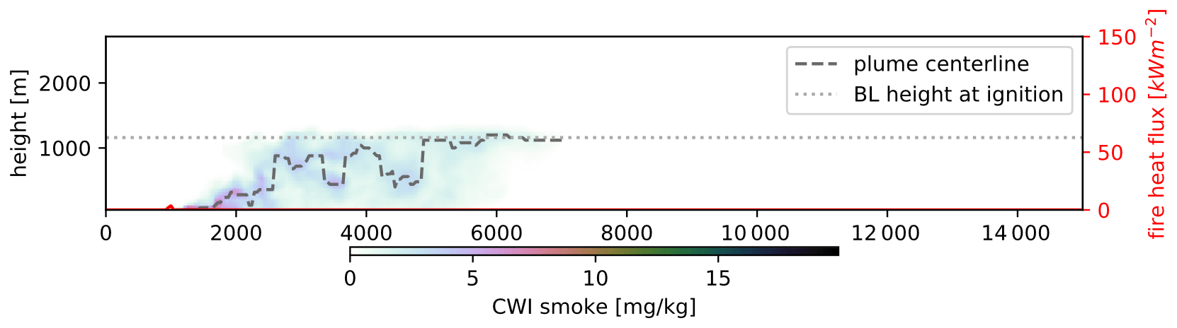
Figure B1 Fixed aspect ratio plot of CWI smoke from a sample non-penetrative plume (W5F8R3). Plume centerline and z_i shown in dashed and dotted grey, respectively.

Red cells in Table B2 highlight simulations that were completed but subsequently excluded from analysis presented in Sect. 3. This was done based on visual inspection of LES fields. There were two possible reasons for exclusion: (i) the plume reached the top of the domain or (ii) the plume appeared to be non-penetrative. In the former case, it is questionable whether the fields are physical, as the plume could potentially be affected by the absorbing layer near domain top, designed to prevent numerical instability. The latter rendered the plume irrelevant for the purpose of analysis presented in Sect. 3. These non-penetrative runs, however, were included for testing the plume classification method presented in Sect. 5.1.

Table B1 Combinations of test conditions resulting in penetrative plumes, as captured by the LES datasets. Green cells highlight fireline length condition (L) runs. The intensity of the blue color corresponds to the number of runs for fuel condition (F) represented by the cell. Row W5 is expanded in Table B2 below.

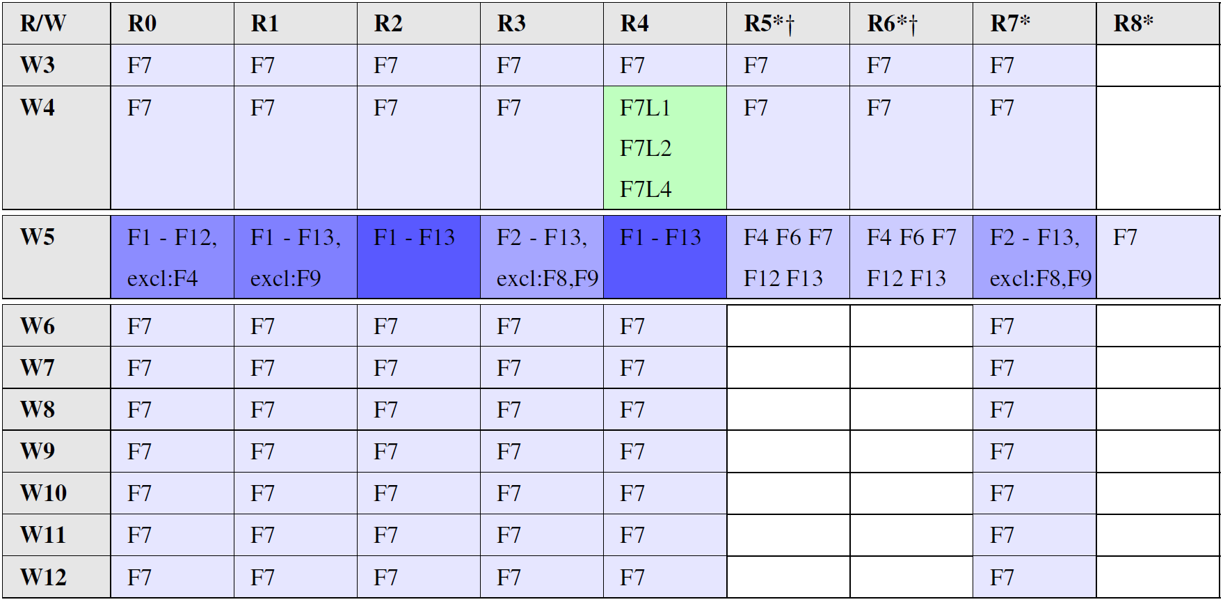
^* Deep domain (5 km). ^† Extended runtime (30 min).

Table B2 Tested combinations of fuel and ABL conditions (all blue and pink colored cells).

^* Deep domain (5 km). ^† Extended runtime (30 min).

Appendix C: Identifying quasi-stationarity

We define the quasi-stationary downwind region for each plume based on two factors: the height of the centerline and tracer concentration gradient along the centerline. Our filter attempts to extract only those portions of the downwind CWI smoke distribution where both of these factors are changing slowly.

First, we remove the effect of random turbulent oscillations by applying a smoothing function (Savitzky–Golay filter provided by SciPy library with polynomial order set to 3) to both the concentration gradient along the centerline and the centerline height. We vary the size of the smoothing window as a function of mean ambient wind condition W, such that $\text{window}\mathit{\_}\text{length}=\text{max}(W\cdot \mathrm{10}+\mathrm{1},\mathrm{51})$ grid points.

The filter then applies the following criteria to extract quasi-stationary regions:

• A smoothed tracer concentration along the plume centerline varies by less than 10 % of the maximum concentration gradient,

• The smoothed centerline height varies by less than a 100 m,

• The location is downwind of the maximum tracer concentration gradient,

• The location is at least 10 grid points away from the maximum in smoothed and non-smoothed centerline height,

• The location is at least 50 grid points away from the downwind endpoint of the centerline.

The above thresholds were determined through an informal sensitivity analysis (not shown), based on the filter's ability to effectively identify regions of near-stationary plume centerline height for all simulations in our dataset.

Appendix D: Estimating model input parameters

Summarized in Table D1 are parameters associated with an iterative solution for z_CL using Eq. (8). Below is our approach to estimating these parameters from LES data.

As noted above, we consider the problem in crosswind direction. Given a three-dimensional fire of an arbitrary shape (e.g. Fig. 2b) and an ambient atmospheric sounding, we first average the fire kinematic heat flux for all ignited cells (where heat flux >1 kW m⁻²) over the crosswind (y) direction at the surface (red line in Fig. 2a). Due to surface wind shear, this direction may differ from the one used for calculating CWI smoke concentrations (as shown in Sect. 4.3). To obtain fireline intensity parameter I, we numerically integrate the crosswind averaged heat fluxes over the depth of the fireline in the along-wind (x) direction.

We use pre-ignition potential-temperature profile (i.e. the ambient environment upwind of the fire) averaged over the entire LES domain as an environmental sounding. All model fields are interpolated to have a 20 m vertical increment. z_i is defined as the height of the strongest environmental lapse rate gradient, and $z_s=\frac{\mathrm{3}}{\mathrm{4}}{z}_i$, based on an informal model sensitivity analysis (not shown). The exact choice of z_s has little effect on model performance as long as it remains within the upper portion of the uniform potential-temperature well-mixed layer.

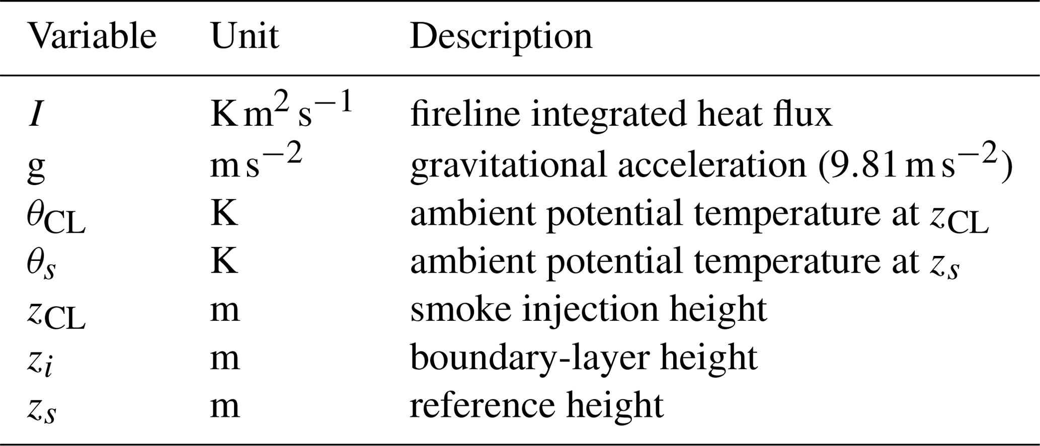
Table D1 Variable descriptions and units used in the smoke injection model.

The values of θ_s and θ_CL are then determined from the pre-ignition sounding for each simulation using the definitions of z_s and z_CL (as described in Sect. 2.3).

Appendix E: Iterative solution for z_CL

The numerical implementation of our iterative solution using SciPy's fsolve function (scipy.optimize.fsolve) is as follows. We rewrite bias-corrected Eq. (8) into an input function toSolve as

$$\begin{array}{}\text{(E1)}& \begin{array}{rl}\text{toSolve}& =\text{lambda }z:z-B_{\mathrm{1}}(z_s+C{\left[{\displaystyle \frac{g\left(T\mathrm{0}\left[\text{int}\left(\frac{z}{\mathrm{d}z}\right)\right]-{\mathit{\theta }}_s\right)}{{\mathit{\theta }}_s(z-z_s)}}\right]}^{-\frac{\mathrm{1}}{\mathrm{2}}}\\ & {\left[{\displaystyle \frac{gI(z-z_s)}{{\mathit{\theta }}_s{z}_i}}\right]}^{\frac{\mathrm{1}}{\mathrm{3}}})-B_{\mathrm{2}},\end{array}\end{array}$$

where C=1.005, B₁=0.924 and B₂=116.417 are bias correction parameters; T0 is the potential-temperature sounding vector; dz is the vertical step; and int() is a standard Python function converting the bracketed value into an integer.

A possible issue for some solvers is that we are, effectively, iterating over the vertical index of the column vector T0 corresponding to z_CL. As the numerical solver attempts to converge on a solution, it may query a non-existent index and fail. We are able to obtain a fast and consistent performance by ensuring we set z_i as the initial guess for z_CL and by minimizing the initial step bound option of the solver:

$$\begin{array}{}\text{(E2)}& {\displaystyle }{\displaystyle }{z}_{\text{CL}}=\text{fsolve}(\text{toSolve},z_i,\text{factor}=\mathrm{0.1}).\end{array}$$