the Creative Commons Attribution 4.0 License.
the Creative Commons Attribution 4.0 License.
 | 17 Sep 2021
Ice and mixed-phase cloud statistics on the Antarctic Plateau
William Cossich
Davide Magurno
Michele Martinazzo
Gianluca Di Natale
Luca Palchetti
Giovanni Bianchini
Massimo Del Guasta
Statistics on the occurrence of clear skies, ice clouds, and mixed-phase clouds over Concordia Station, in the Antarctic Plateau, are provided for multiple timescales and analyzed in relation to simultaneous meteorological parameters measured at the surface. Results are obtained by applying a machine learning cloud identification and classification (CIC) code to 4 years of measurements between 2012–2015 of downwelling high-spectral-resolution radiances, measured by the Radiation Explorer in the Far Infrared – Prototype for Applications and Development (REFIR-PAD) spectroradiometer. The CIC algorithm is optimized for Antarctic sky conditions and results in a total hit rate of almost 0.98, where 1.0 is a perfect score, for the identification of the clear-sky, ice cloud, and mixed-phase cloud classes. Scene truth is provided by lidar measurements that are concurrent with REFIR-PAD. The CIC approach demonstrates the key role of far-infrared spectral measurements for clear–cloud discrimination and for cloud phase classification. Mean annual occurrences are 72.3 %, 24.9 %, and 2.7 % for clear sky, ice clouds, and mixed-phase clouds, respectively, with an inter-annual variability of a few percent. The seasonal occurrence of clear sky shows a minimum in winter (66.8 %) and maxima (75 %–76 %) during intermediate seasons. In winter the mean surface temperature is about 9 ∘C colder in clear conditions than when ice clouds are present. Mixed-phase clouds are observed only in the warm season; in summer they amount to more than one-third of total observed clouds. Their occurrence is correlated with warmer surface temperatures. In the austral summer, the mean surface air temperature is about 5 ∘C warmer when clouds are present than in clear-sky conditions. This difference is larger during the night than in daylight hours, likely due to increased solar warming. Monthly mean results are compared to cloud occurrence and fraction derived from gridded (Level 3) satellite products from both passive and active sensors. The differences observed among the considered products and the CIC results are analyzed in terms of footprint sizes and sensors' sensitivities to cloud optical and geometrical features. The comparison highlights the ability of the CIC–REFIR-PAD synergy to identify multiple cloud conditions and study their variability at different timescales.
- Article
(5896 KB) - Full-text XML
- BibTeX
- EndNote


The polar regions present several challenges for meteorology and climatology studies (Walsh et al., 2018). These regions are crucial components of the Earth's radiation budget (ERB) (Liou, 2002; Kiehl and Trenberth, 1997) since they generally emit more energy to space in the form of infrared radiation than what is absorbed from sunlight, thereby behaving as heat sinks. Modeling studies have shown that changes in cloud properties (e.g., cloud amount, cloud thermodynamic phase, cloud height, cloud optical thickness) over Antarctica may impact different regions in the globe, highlighting the importance of Antarctic clouds for the global climate system (Lubin et al., 1998). However, obtaining measurements of cloud properties in the Antarctic continent is still a challenge (Silber et al., 2018; Lubin et al., 2020), especially in its interior (Town et al., 2005; Lachlan-Cope, 2010; Bromwich et al., 2012). Observations from synoptic weather stations require an experienced observing staff and sometimes become unavailable during “white-out” conditions caused by blowing snow. Analysis of satellite measurements from both active and passive sensors must account for a number of problems in inferring the cloud properties. One issue is that the cloud radiative properties tend to be very similar to those of the background (the snow or ice surface). Optically thin cirrus clouds are often present in the Antarctic Plateau (King and Turner, 1997) but are difficult to identify and analyze due to their small cloud signals (the difference between cloudy and clear-sky radiances). Measurements become problematic during the long polar night (King and Turner, 1997), and some stations reduce the observing frequency in the winter time (Bromwich et al., 2012). Observations at solar wavelengths are not available for about half of the year, thus reducing the overall ability to recognize the presence of cloud layers and to derive their physical and optical features. Measurements at longer wavelengths (i.e., in the infrared, IR) are available regardless of solar illumination, but, frequently, the cloud top temperature is similar to the ice surface temperature (King et al., 1992; King and Turner, 1997; Bromwich et al., 2012), and the cloud identification is thus difficult from passive satellite observations.
Active remote sensing techniques have been very helpful in overcoming the limitations of the passive instruments in polar regions. Adhikari et al. (2012) investigated the seasonal and inter-annual variabilities in the vertical and horizontal cloud distributions over the southern high latitudes poleward of 60∘ S, using observations from CloudSat and Cloud–Aerosol Lidar and Infrared Pathfinder Satellite Observation (CALIPSO) satellites between June 2006 and May 2010. They found that the Antarctic Plateau has the lowest cloud occurrence of the Antarctic continent (<30 %). The sensors on board the aforementioned satellites have also been used to investigate macro- and microphysical Antarctic cloud properties (Verlinden et al., 2011; Adhikari et al., 2012; Listowski et al., 2019; Ricaud et al., 2020). Nevertheless, satellite active sensors are not lacking in problems when used for cloud detection in polar regions. For example, Chan and Comiso (2011, 2013) discuss the difficulties encountered by the Cloud Profiling Radar (CPR), on CloudSat, and the Cloud–Aerosol Lidar with Orthogonal Polarization (CALIOP), on CALIPSO, in detecting low-level clouds in the Arctic. The difficulties arise from the CloudSat coarse vertical resolution (about 500 m) and its limited sensitivity (low signal-to-noise ratio) near the surface and in the case of CALIOP are due to the geometrically thin nature of the cloud and its surface proximity. Bromwich et al. (2012) present a review of Antarctic tropospheric clouds. They discuss the instruments and methods to observe Antarctic clouds and the current datasets available. The authors highlight that there are relatively few measurements of clouds in the Antarctic, especially in the interior. They also indicate that better and more frequent remote sensing and in situ observations are needed.
The selection of the FORUM project (Palchetti et al., 2020) in 2019 as the ninth Earth Explorer mission by the European Space Agency (ESA) has revitalized studies in the far-infrared (FIR) part of the spectrum, approximately covering the 100–700 cm−1 band. Many studies have shown that the FIR can be used to complement standard remote sensing measurements performed in the mid-infrared (MIR) and improve cloud detection, classification, and inference of cloud properties (Rathke et al., 2002; Palchetti et al., 2016; Di Natale et al., 2017; Maestri et al., 2019a). Moreover, ground-based remote sensing spectral upwards-looking measurements are very useful to determine the cloud properties relevant to the energy budget (Mahesh et al., 2001; Cox et al., 2014; Di Natale et al., 2020).
This study is performed in this context and exploits a unique dataset derived from FIR and MIR downwelling spectral radiances measured at Concordia Station, Dome C, in the middle of the Antarctic Plateau. The measurements are performed by means of the Radiation Explorer in the Far Infrared – Prototype for Applications and Development (REFIR-PAD) Fourier transform spectroradiometer (Bianchini et al., 2019) in the scope of the projects Radiative Properties of Water Vapor and Clouds in Antarctica (PRANA) and Concordia Multi-Process Atmospheric Studies (CoMPASs), within the Italian National Program for Research in Antarctica (PNRA; Palchetti et al., 2015). These projects represent the first long-term field campaigns to collect high-spectral-resolution radiances in the FIR, with continuity for an extended period (measurements started in 2012). REFIR-PAD is installed inside an insulated shelter, named the Physics Shelter, together with a backscattering lidar (abbreviation of light detection and ranging). The lidar detects backscattering and depolarization signals up to 7 km above the surface. Besides these measurements, the Antarctic Meteo-Climatological Observatory installed at Concordia (http://www.climantartide.it/, last access: 14 September 2021) provides data from an automatic weather station (AWS) and from daily radiosonde launches. These measurements are analyzed and correlated to the meteorological conditions observed at Concordia Station and are considered representative of a large area of East Antarctica because of the horizontal uniformity in the Antarctic Plateau.
Recently, Maestri et al. (2019b) presented an algorithm to identify and classify clouds based on principal component analysis of IR radiance spectra at high spectral resolution. The cloud identification and classification (CIC) is a fast machine learning algorithm able to perform a cloud detection and classification, exploiting spectral variations in IR radiance signals. CIC can account for spectral radiance from the full IR spectrum including the MIR and FIR. The algorithm analyzes a distribution of the so-called similarity index, which is a parameter defining the level of closeness between the analyzed spectra and the elements of specific classes that are defined with training sets.
In this study, the CIC algorithm is applied to REFIR-PAD downwelling radiances to detect and classify Antarctic clouds between 2012 and 2015. The main goal of this effort is to obtain statistics on clear-sky and cloud occurrence as well as the investigation of the diurnal cycle and seasonality of clouds in the Antarctic Plateau. Both ice and mixed-phase clouds have been considered, the latter consisting of a supercooled liquid water layer that, in general, may have ice particles present either above or below (usually precipitating in this case).
The algorithm is first applied to a test set so that the CIC performances are assessed. The excellent classification scores obtained in the testing phase provide a solid base for the application of the CIC to the entire dataset. In this study, an effort is made to link the meteorological state of the atmosphere to the cloud occurrence.
The paper is organized as follows. Section 2 describes the instrumentation and measurements performed at Concordia Station. Section 3 introduces the CIC algorithm, its setup, and optimization to identify and classify clouds. Section 4 discusses the cloud occurrence results at different timescales. The study is summarized in Sect. 5, where conclusions are drawn.

Figure 1Antarctica elevation map, with Concordia Station indicated by a red star.
Concordia Station is an Antarctic research base located at Dome C over the Antarctic Plateau (75∘06′ S, 123∘23′ E; 3.230 m a.m.s.l.), in the East Antarctic region (Fig. 1). The station opened in 2005 as part of an international cooperation project between the Italian National Program for Research in Antarctica (PNRA) and the French Polar Institute Paul-Émile Victor (IPEV). A detailed description of the instrumentation available in the PRANA and CoMPASs experiments at Concordia Station is given in Palchetti et al. (2015). A brief overview of the instruments and measurements made between 2012 and 2015 is provided in what follows.
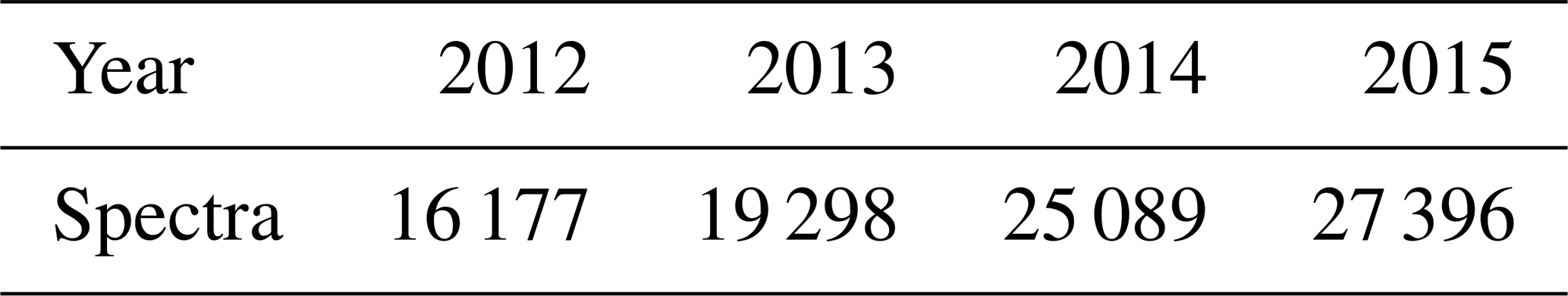
Spectral measurements of the downwelling radiance are performed by REFIR-PAD, which provides spectrally resolved zenith-looking radiance measurements in the range 100–1500 cm−1, with a 0.4 cm−1 spectral resolution, thus covering a large part of the atmospheric longwave emission, including both the FIR and part of the MIR region. The instrument points at the zenith through a 1.5 m chimney. The measurement sequence to obtain one complete spectrum is made of four calibration acquisitions, in which the instrument looks at the internal reference blackbody sources, and four sky observations. Each single acquisition takes about 80 s. The entire sequence has a duration of about 14 min: 5.5 min of sky observations, 5.5 min of calibrations, and delays for detector settling after scene changes (Palchetti et al., 2015). REFIR-PAD is a fast-scanning spectroradiometer with signals acquired in the time domain and resampled in postprocessing at equal intervals in optical path difference. It has been designed to operate with uncooled detectors and optics. The instrument operates full-time, with alternating cycles of 5–6 h of measurements and 1–3 h of analysis. It is installed in the Physics Shelter, located 500 m southward from the main station, in what is called the clean-air area, where the predominant winds keep the air clean from the exhaust plume of the Concordia power generator. Between the years 2012 and 2015, a total of 87 960 spectra were analyzed. The spectra annual distribution is reported in Table 1.
Since 2005, Concordia Station has provided hourly measurements of air temperature, pressure at the surface level, relative humidity, wind speed, and wind direction. The snow temperature is measured at different depths from 5 cm to 10 m. These measurements began in December 2012. Radiosondes (Vaisala RS92) have been routinely released every day at 12:00 UTC since 2006. They reach an altitude of about 18 km in wintertime and about 25 km in the summer. All these data are made available by the Antarctic Meteo-Climatological Observatory, and a subset of them is used in this study.
Atmospheric backscattering and depolarization ratio (cross-polarized over parallel-polarized total signal) profiles are measured by a lidar every 5 min (Palchetti et al., 2015). The instrument (http://lidarmax.altervista.org/englidar/Antarctic%20LIDAR.php, last access: 14 September 2021) is a Hamamatsu analog photo-multiplier tube, operating a Quantel laser (Brio) at 532 nm with a biaxial configuration (10 cm off-axis) and nominal laser aperture of 1 mrad full angle. The lidar telescope has refractive optics with 10 cm diameter and 30 cm focal length, with a field of view of approximately 2 mrad full angle. An interference bandpass filter of 0.15 nm bandwidth is applied. The signal is averaged over 1000 laser shots. Measurements range from 30 to 7000 m above the surface, with 7.5 m vertical resolution. The line of sight is 4∘ off-zenith to avoid possible ambiguity between liquid-phase clouds and oriented ice plates (Ricaud et al., 2020). The lidar operates through a window to enable measurements in all weather conditions.
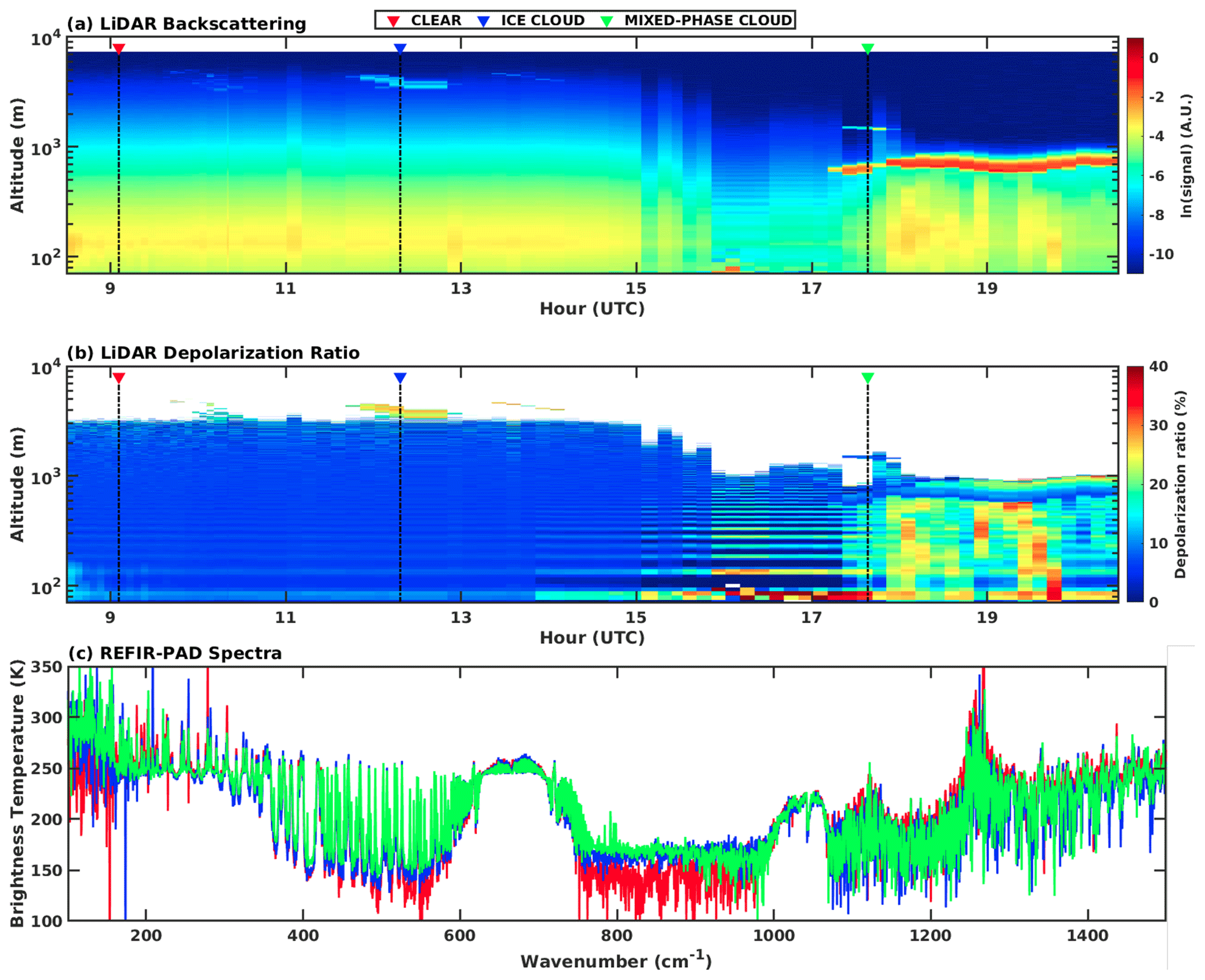
Figure 2(a) Lidar backscattering and (b) depolarization ratio for 2 January 2013. (a, b) Different sky conditions are highlighted by a vertical dashed line. A red triangle indicates clear sky, a blue triangle is used for ice clouds, and a green triangle is used for mixed-phase clouds. (c) REFIR-PAD spectra corresponding to the three sky conditions highlighted in the upper and middle panels. The same color code is used.
Definition of classes
A subset of REFIR-PAD data, comprising 1928 spectra, is co-located with lidar measurements. The co-location criterion is defined by the time of measurements: each REFIR-PAD spectrum is associated with the lidar data that are closest in time. Co-located measurements are used to classify the REFIR-PAD spectra. For these cases, cloud layers are detected from the analysis of the backscatter profiles, and the depolarization ratio is used to determine the thermodynamic phase of the particles. The classified spectra are then used to set up training and test sets as described in more detail in the next section. In the Antarctic environment the determination of cloud thermodynamic phase is not trivial. According to Liou and Yang (2016), liquid water droplets retain the polarization state of the incident energy, while the light beam backscattered from non-spherical ice particles is partially depolarized as a result of internal reflections and the transformation of coordinate systems governing the electric vector. A theoretical analysis performed by the same authors shows that in the presence of a liquid water cloud the depolarization remains at about 2 %–4 %, whereas radiation backscattered from non-spherical ice particles is strongly depolarized, varying between 30 % and 40 %. However, the threshold to determine the water physical state in real clouds can vary depending on the atmosphere and the cloud microphysical parameters. Sassen and Hsueh (1998) evaluate ground-based lidar data in the presence of contrail cirri during the Subsonic Aircraft: Contrail and Cloud Effects Special Study (SUCCESS) field campaign. They found depolarization ratios in persisting contrails ranging from about 0.3 to 0.7. Freudenthaler et al. (1996) observed depolarization ratios of 0.1 to 0.5 for contrails with temperatures ranging from −60 to −50 ∘C, depending on the stage of their growth. In this study, a depolarization ratio of 0.15 is used as a threshold (as indicated by Sassen, 1991) for the discrimination of the liquid water clouds and ice clouds over Concordia Station. The value accounts for possible increases due to multiple-scattering effects as discussed below.
An example of lidar observations for clear sky (red triangle), ice clouds (blue triangle), and mixed-phase clouds (green triangle) is provided in the upper (backscattered signal) and middle (depolarization ratio) panel of Fig. 2. The lower panel of the same figure provides the corresponding REFIR-PAD spectra. In clear-sky conditions, the lidar backscattering signal decreases with altitude, while the signal increases in the presence of cloud particles. As shown in the figure, clouds can be composed of multiple layers, each one with different depolarization features. When the depolarization ratio is higher than 15 %, the cloud is classified as an ice cloud (blue triangle). For lower values of the depolarization ratio, it is assumed that the layer contains the liquid phase, and the cloud is categorized as a mixed-phase cloud (green triangle). The 15 % depolarization ratio value is selected to account for the impact of multiple scattering within liquid clouds. It is observed that in the presence of mixed-phase clouds the depolarization ratio shows very small values at the cloud base, characteristics of liquid spheres, and increases towards values typical of ice crystals near the cloud top. An increase is, in part, intrinsically related to liquid water layers, where multiple scattering determines a depolarization that gradually increases with the depth of penetration. For this reason, in some conditions, the phase of the upper part of the cloud cannot be unambiguously defined based on the analysis of the depolarization ratio profile only. Nevertheless, the presence of the liquid phase at the bottom is unequivocally identified, and the cloud is categorized as mixed-phase. The occurrence of precipitating ice crystals from mixed-phase cloud layers is not infrequent, even if in very small quantities.
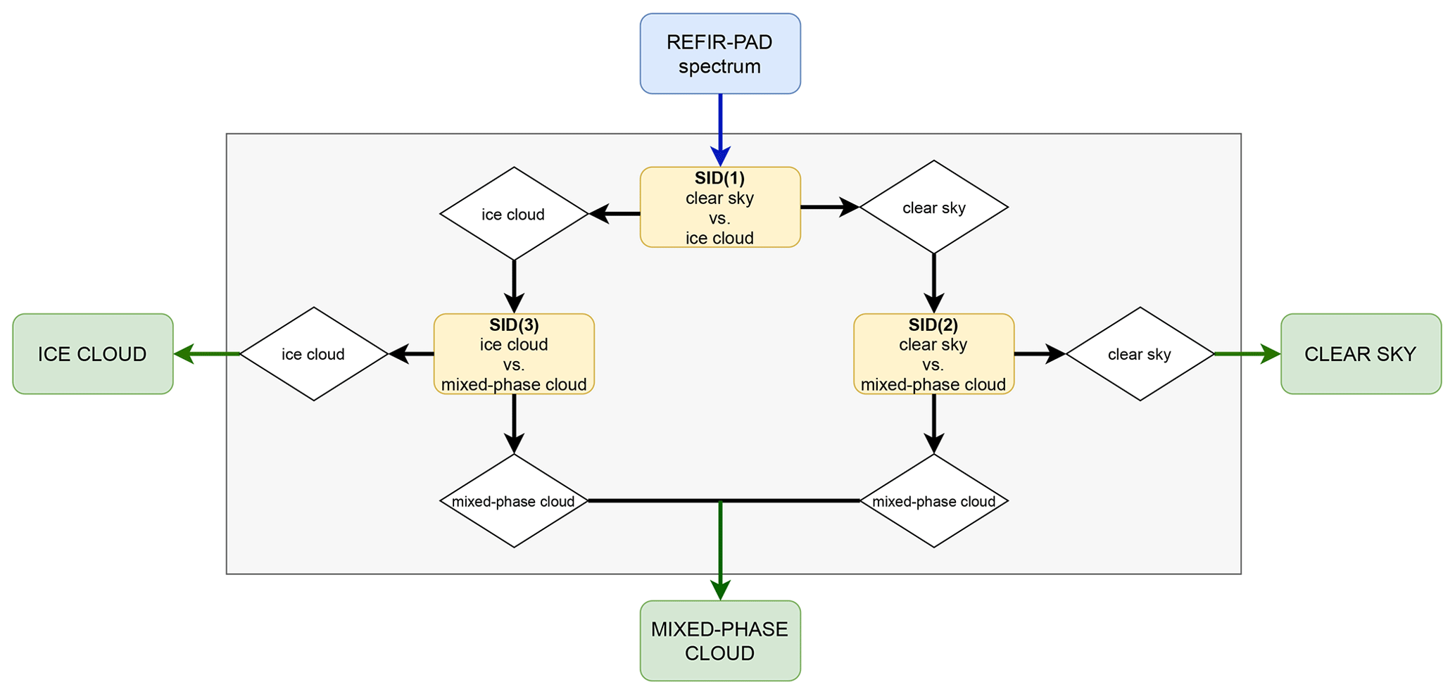
Figure 3Logical diagram of the classification process performed by the CIC algorithm for the definition of the clear-sky, ice cloud, and mixed-phase cloud classes.
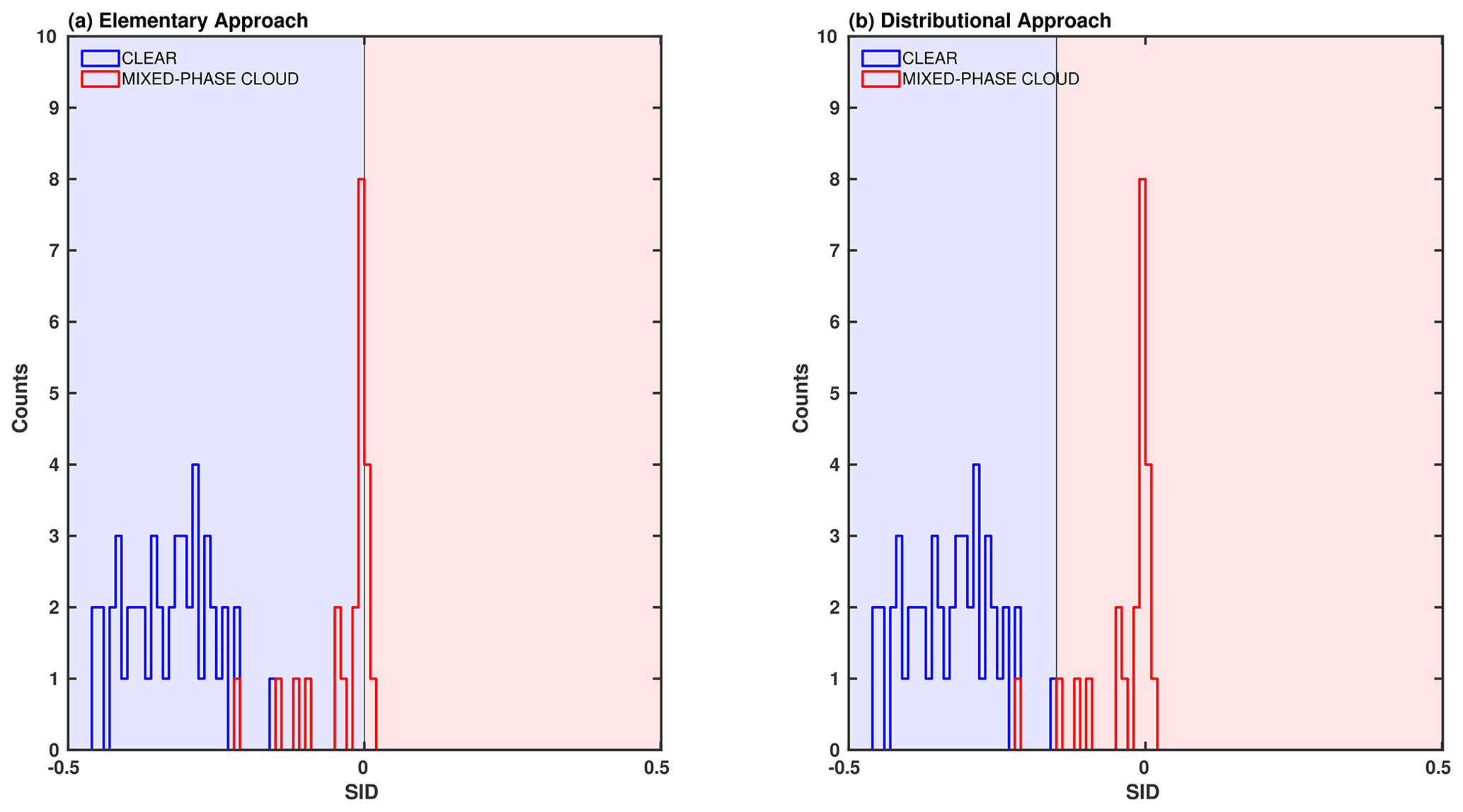
Figure 4Example of (a) the CIC elementary approach and (b) the distributional approach applied to the training set elements of clear sky (49 spectra) and mixed-phase clouds (22 spectra) in the warm season (November–March). The clear-sky (blue histogram) and the mixed-phase cloud (red histogram) training set elements are classified according to the SID as clear-sky (shaded blue area) or mixed-phase cloud (shaded red area) scenes. Only 76 % of the spectra are correctly classified using the elementary approach, while 99 % of the spectra are correctly classified using the distributional method.
The Cloud Identification and Classification (CIC) is a machine learning algorithm, based on the principal component analysis (PCA), that is able to classify an input spectrum (ℒ) as representative of a specific class, characterized by the elements contained in multiple groups of spectra used as training sets (TSs). The algorithm is based on the analysis of the measured spectra only and does not require any ancillary information or forecast model output data for the classification. The classification accounts for the spectral features of the observed brightness temperature (BT) compared to the characterizing spectral features of each training set. A brief description of the algorithm is provided below; we recommend the reference article by Maestri et al. (2019b) for a full description of the CIC.
For each class X (i.e., clear-sky, ice cloud, and mixed-phase) a set of spectra is used to set up a training set defining the variability within the class:
where is the wavenumber, and refers to the jth element (spectrum) of the TS. The information content of the TSs is evaluated by computing the eigenvalues (λ) and the eigenvectors (ϵTS) of the TS covariance matrices:
The procedure also accounts for a spectral noise removal operation. This is performed by accounting only for a limited number of principal components, defined by Turner et al. (2006) as the first P0 eigenvalues, out of P total components that minimize the indicator function:
where refers to the pth principal component, and the real error RE is defined as
Each input spectrum ℒ is then analyzed by defining the extended training sets (ETSs) that are the original TSs plus the input spectrum itself,
and by computing the eigenvectors (ϵETS) of each ETS covariance matrix.
The classification is performed through a parameter called similarity index (SI) that evaluates the variation in the information content in the ETS with respect to the original TS (for each class):
The SI is a normalized index, where a value close to 1 means high similarity, and a value close to 0 means low similarity. As an example, if the input spectrum is measured in clear-sky conditions, the information content of the ETSCLEAR would be similar to the original TSCLEAR, and their eigenvectors will also be very similar due to the low additional information content from the input spectrum.
For this study, as previously indicated, three classes are defined: clear sky, ice clouds, and mixed-phase clouds. Consequently, three training sets are prepared, each one containing spectra representative of that particular class. For each observation the operation described in Eq. (6) is performed for 2 classes at a time. In our case, three SIs are obtained, derived from the mutual comparison of the three classes. From these, a vector of similarity index differences (SIDs) is defined:
The classification of the input spectrum is performed in accordance with the logical diagram of Fig. 3. The diagram shows the comparison between specific couples of SI (yellow boxes). The partial results of each comparison are represented by white boxes. If one class prevails over the other two, a classification is reached, and the final output is provided (green boxes in the figure).
The comparison between the SI of the classes is called the elementary approach. This methodology is based on a very simple classificator, the SID, which works properly when each class is characterized by specific spectral features that make the elements of the class easily distinguishable from those pertaining to other classes. This is clearly very difficult to attain for some classes such as, for example, the clear-sky class and the cirrus cloud class. The classification of clouds over the Antarctic Plateau is particularly challenging, primarily because of the generally low cloud optical depths whose IR spectral characteristics are very similar to those of the clear sky. The selection of the spectra contained in each training set is crucial as it is in every classification algorithm. In fact, the selected elements must represent the entire class characteristics and variability to perform a correct classification.
Maestri et al. (2019b) suggested that better results can be obtained when a classificator optimization is performed a priori by using a methodology called distributional approach. When applied to a set of observations, a perfect classifier would ideally generate a bimodal SID distribution for each comparison between two classes, splitting the elements in two separate groups. This class separation is difficult to achieve in reality, and the amount that elements overlap depends on many factors, including the spectra used to define the training sets. To mitigate the issue, the CIC is applied separately to each training set element. Based on the result for each spectrum of known class, an evaluation can be made for the SID distribution for the entire set of each class. Through this analysis of the SID distributions, an optimal SID delimiter can be defined to maximize the correct classification of the training set elements. The delimiters, which can be different from zero, are set according to the classification results to optimize the algorithm performance. An example of the SID distribution based on the training set spectra and of the elementary and the distributional approaches is provided in Fig. 4. The CIC is applied to the training set spectra of clear sky and mixed-phase clouds. The elementary method (left panel) classifies as clear sky (shaded blue area) all the spectra with SID≤0 and as mixed-phase cloud (shaded red area) all the spectra with This methodology misclassifies some of the mixed-phase cloud training set spectra (red histogram). The distributional method (right panel) maximizes the classification performance by defining a new delimiter between clear-sky and mixed-phase cloud scenes. In this example, the new delimiter is set at SID so that most of the TS spectra are correctly classified. See Maestri et al. (2019b) for a description of the computation of the delimiter. Once the delimiters (DELs) are defined for each class couplet, the classification is performed by using a corrected similarity index difference (CSID):
The entire classification procedure, schematically described in Fig. 3, is then performed by the new classifier CSID in place of the SID. Due to the better performance, the distributional method is preferred and applied in this study.
Table 2Number of spectra used in each TS according to the macro-season. The total number of spectra used in the TS is 202.
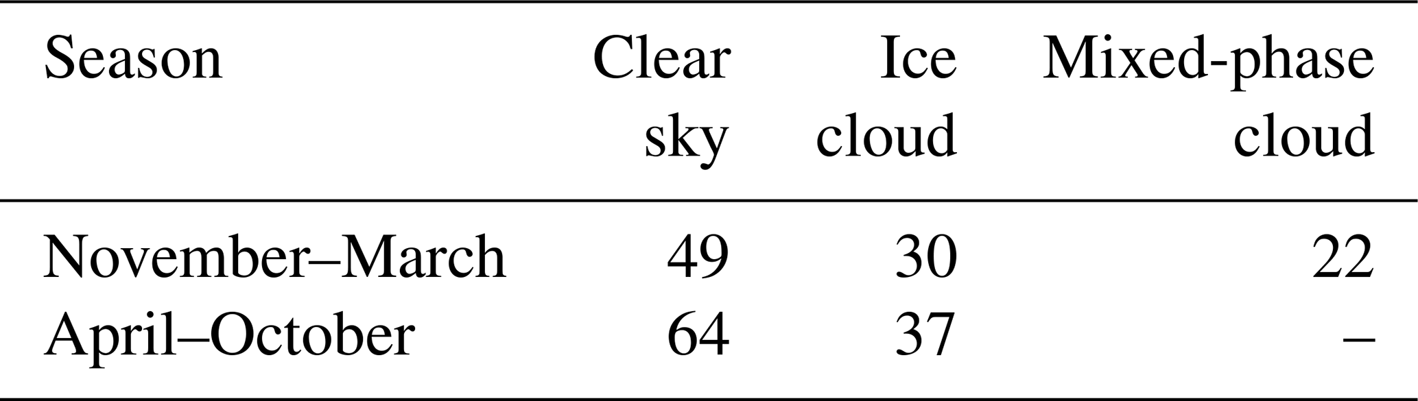
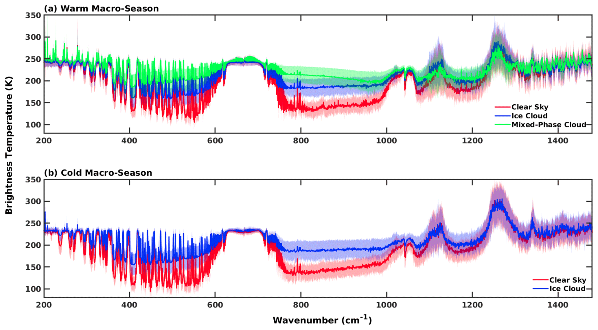
Figure 5Average BT (solid line) ±1 standard deviation (shaded area) for TS elements of the (a) warm and (b) cold macro-seasons.

Figure 6Threat scores for the test set as a function of different spectral intervals ingested by the CIC algorithm. The (a) “all classes” threat score is a weighted mean of the threat scores computed for each class: (b) clear sky, (c) ice cloud, and (d) mixed-phase cloud.
3.1 Training and test sets
Spectra used to populate the training sets are chosen from a set of pre-classified observations. The identification is performed by the co-located lidar backscatter and depolarization profiles in accordance with the criteria described in Sect. 2. Each training set contains a limited number of spectra from the REFIR-PAD database, aiming at describing the variability in atmospheric conditions over Concordia Station. Due to the intense variations in the environmental conditions, the training sets are defined for two macro-seasons: a warm season (November–March) and a cold season (April–October). The choice is also supported by the fact that mixed-phase clouds are extremely rare in the cold macro-season. Ricaud et al. (2020) observed the occurrence of supercooled liquid water clouds during the warm macro-season only, with the largest frequency occurring in December and January. Listowski et al. (2019) also observed that the fraction of supercooled liquid-water-containing clouds in the Antarctic Plateau varies between 10 %, in the summertime, and 0 %, in winter. Therefore, three training sets for the warm macro-season are defined: clear sky, ice clouds, and mixed-phase clouds. For the cold macro-season, only the clear-sky and ice cloud training sets are used. Table 2 summarizes the number of spectra for each TS and macro-season. The same spectra are used later (Sect. 4) to perform the classification of the full dataset.
Mean spectra in terms of BT (solid lines) and their standard deviations (shaded area) are presented in Fig. 5 for the training sets used for both macro-seasons. Differences between the mean spectra of the different classes are observed in the window channels located between 400 and 600 cm−1 as well as between 800 and 1000 cm−1. Note that in IR window regions (transparent channels) the standard deviation of the clear-sky spectra is usually lower than that of the cloudy spectra, which account for a wider signal variability in these bands. Furthermore, the clear-sky signal is very low at window wavenumbers, and the measurements can have a very low signal-to-noise ratio.
Once the TSs are defined, the DELs are computed (as described in Sect. 3), and the CIC is ready to ingest the REFIR-PAD spectra and provide their classification. To evaluate the CIC performance and optimize its setup, a test set of 1726 pre-classified spectra collected in 2013 is analyzed. The test set is composed of 559 clear-sky, 1022 ice cloud, and 145 mixed-phase cloud spectra. These spectra were previously classified by using the co-located lidar backscatter and depolarization profiles. An example is provided in Fig. 2. We define the sky condition as that observed when the REFIR-PAD starts its measurement. Then, the spectra are associated with the sky conditions encountered at the beginning of each measurement.
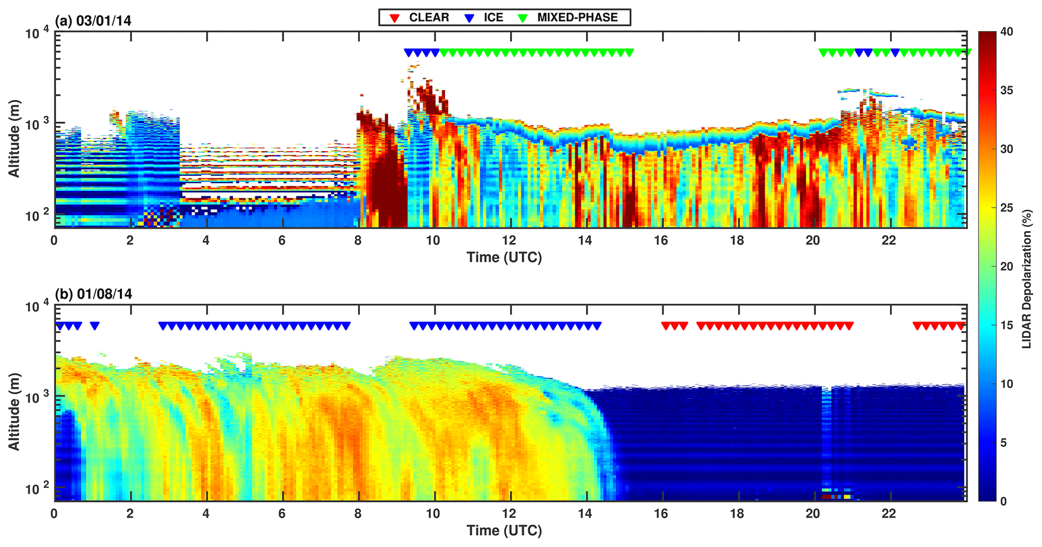
Figure 7Lidar depolarization ratio on (a) 3 January 2014 and (b) 1 August 2014. The triangles mark the REFIR-PAD observations. The color code indicates the CIC classification: red for clear sky, blue for ice clouds, and green for mixed-phase clouds.
3.2 CIC performance and optimization
The CIC algorithm is applied to the test set spectra by accounting for their BT in different spectral intervals. This operation is performed to find the optimal spectral interval that maximizes the classification results for each class (clear sky, ice cloud, mixed-phase cloud). Multiple runs of the CIC algorithm are performed on the same test set by applying it to different spectral ranges. Specifically, the starting wavenumber is moved in steps of 20 cm−1 in the 200–600 cm−1 band, and the ending wavenumber is moved between 960 and 1480 cm−1. Note that, as discussed in Maestri et al. (2019b) and Magurno et al. (2020), the spectral interval 620–670 cm−1 is excluded from the analysis.
The algorithm performance during this process is assessed by evaluating the threat score (ThS). A confusion matrix is used to compute the ThS of each class and for each considered spectral interval. Each individual spectrum can be classified correctly as a member of its class (i.e., class A) or incorrectly as a member of a different class (i.e., class B or C). With this symbolism, the spectrum classification is interpreted in terms of the following.
- –
True positive (TP): the spectrum belongs to class A, and it is properly classified in class A.
- –
True negative (TN): the spectrum does not belong to class A, and it is properly classified in its class of pertinence (B or C).
- –
False positive (FP): the spectrum belongs to class B or C, but it is misclassified in class A.
- –
False negative (FN): the spectrum belongs to class A, but it is misclassified in class B or C.
Given the above possibilities, for each class the threat score is defined as
which accounts for the correctly classified spectra (TP) in the class and penalizes all the misclassified occurrences (FN and FP). A ThS value of 1 means that there are no misclassified spectra.
Based on the results obtained for each of the combinations of starting and ending wavenumbers, the ThS is calculated for each class (clear sky, ice cloud, mixed-phase cloud). The weighted mean ThS values, which account for the total number of cases in each class, are also calculated. In the upper left panel (a) of Fig. 6 the mean ThSs are plotted as a function of the starting and ending wavenumbers. The other panels in this figure (b, c, d) show results for the three specific classes. The ThS values span from 0.487 to 0.966 in accordance with the selected interval and the given class. For intervals ending with wavenumbers larger than 1140 cm−1, the ThS decreases considerably for all the classes. This is likely associated with the noise of the REFIR-PAD sensor, which increases considerably above 1200 cm−1 and degrades the classification results. When the ending wavenumber is set to values between 980 and 1080 cm−1, the ThS is very high (larger than 0.9) for all the starting wavenumbers below 400 cm−1, both for clear sky and ice clouds. The spectral interval 380–1000 cm−1 performs the best for classification of both clear sky and ice clouds, where the ThS values are 0.963 and 0.966, respectively. The classification of mixed-phase clouds is slightly less robust compared to the other two classes, and the best spectral interval is 540–1020 cm−1 with a ThS of 0.927. Typically, mixed-phase clouds are associated with more humid conditions than ice clouds and, frequently, with precipitation of thin ice crystals. For these reasons, the inclusion of the smallest wavenumbers (associated with the less transparent part of the FIR) does not maximize the classification of mixed-phase clouds.
When accounting for all the classes, the best performing spectral range for clear and cloud identification and classification is the 380–1000 cm−1 interval. The result is dependent on sensor characteristics, and for this study it is specifically driven by the REFIR-PAD spectral resolution and noise features. The optimal interval for the classification is also dependent on many other parameters, among which are the type and number of classes considered, the observation geometry (e.g., satellite- or ground-based), the observing location, and the mean atmospheric conditions. Because the water vapor content is extremely low, the ground-based measurements on the Antarctic Plateau allow the full exploitation of the FIR spectral range. These channels would be totally opaque for upward observations in regions of increased water vapor content such as the tropics. The selected spectral range (380–1000 cm−1) highlights the fundamental role of the FIR part of the spectrum in the cloud identification and classification.
The results of the CIC classification applied to the test set using the 380–1000 cm−1 are summarized in Table 3. The table reports the number of spectra per class in the test set, the CIC hit rates (HRs) and misclassified spectra in percentage, and the threat scores. The HR for a class (i.e., A) is defined as
where is the number of occurrences of the class A that are correctly identified by the CIC (corresponding to the TP in the confusion matrix). is the total number of elements in class A of the dataset and corresponds to TP+FN of the class A.
The overall performance is that almost 98 % of spectra are correctly classified. Only a small percentage (less than 1 %) of cloudy spectra (ice clouds plus mixed-phase clouds) are misclassified as clear sky, and about 2 % of the clear-sky spectra are erroneously identified as ice clouds. Note that in the case of mixed-phase clouds the CIC is able to identify the presence of the cloud in 99.3 % of the cases even if for 8.3 % the cloud phase is classified as ice instead of mixed-phase. This is actually a very reasonable performance considering that, as noted before, most of the mixed-phase clouds are composed of a layer of super-cooled liquid phase near the cloud base and, likely, ice-phase particles close to the cloud top as suggested by the large values of the depolarization ratio.
Sensitivity studies on the identification of mixed-phase clouds are performed assuming a cloud layer of constant total optical depth of 2 at 900 cm−1, in which the base layer is composed of liquid water, and the upper layer is occupied by ice particles. The relative weight of the two layers to the total optical depth (OD) varies from a completely ice cloud to a completely liquid water cloud. Results (not shown here) demonstrate that for the bottom layer of liquid phase with OD larger than 0.1–0.3 the cloud is identified as mixed-phase; otherwise, it is classified as an ice cloud. This demonstrates that the algorithm is very sensitive to the presence of thin liquid water layers at the cloud base. Nevertheless, it is also possible to incur in situations in which a very thin layer of liquid water is close to a thicker ice layer, and the spectral signal measured at the ground is interpreted by the CIC algorithm as exiting from an ice cloud. Another common situation is the presence of falling ice from mixed-phased cloud layers, as shown in the mid panel of Fig. 2 between 18:00 and 20:00 UTC. Typically, the quantity of the precipitating ice crystals is very small, and the CIC algorithm is able to capture the radiometric signal from the upper liquid water layer, as is shown in the case reported in Fig. 7.
Test set misclassified spectra
Each of the misclassified cases is visually inspected to understand the main causes of error in the CIC classification. It appears that the misclassification of clear sky as ice cloud and vice versa occurs primarily for spectra taken during the cold macro-season. The misclassification in this case is associated with the (a) presence of a very thin cirrus cloud; (b) REFIR-PAD measurements taken over a period of time in which the observed scene is changing (i.e., the measuring time encompasses both clear sky and cloudy sky); or (c) presence of suspended particles near the surface (e.g., diamond dust, wind-blown snow, or combustion products produced by the generator that heats Concordia Station).
During the warm macro-season, a small percentage of mixed-phase clouds are misclassified as either clear sky or ice clouds. In some cases, ice clouds are misclassified as mixed-phase clouds; this happens mostly when the ice cloud spectra are characterized by a high BT in the main window region.
The 380–1000 cm−1 spectral interval is used to run the CIC algorithm over the entire REFIR-PAD dataset, comprising measurements from the year 2012 through 2015. In Fig. 7, the CIC classifications are compared with co-located lidar depolarization data for 2 different days. For each REFIR-PAD observation, the classification is reported as a colored triangle in the upper part of each panel. As previously discussed, low values of lidar depolarization together with large values of the backscattering signal (not shown) indicate the presence of liquid water phase in the cloud layer, while high depolarization values are observed in the presence of ice clouds. The upper panel of Fig. 7 shows the presence of a mixed-phase cloud over Concordia Station from about 10:00 UTC until the nighttime of the 3 January 2014. The presence of the cloud and its thermodynamic phase are correctly identified and classified by the algorithm. Between the hours of 21:00 and 22:30 UTC, CIC identifies a spectral signal characteristic of ice clouds that corresponds to larger values of the depolarization ratio measured by the lidar. On 1 August 2014 (lower panel of Fig. 7), the lidar depolarization shows that the day starts with a precipitating ice cloud, followed by clear-sky conditions from 15:00 UTC. For this case, both the clear sky and the ice cloud are correctly detected by the CIC algorithm.
The results of applying the CIC to the full available REFIR-PAD dataset are provided in terms of percentages, defining the occurrence of each class with respect to the total number of analyzed spectra. An error can be associated with the percentage occurrence, exploiting the HRs derived in the analysis of the test set. With the use of Eq. (10) for the HR definition for the class A:
The number of misclassified spectra () of class A can be written as
Through combination of Eqs. (11) and (12), it is possible to remove the term , which is unknown for results applied to the entire dataset. The following relation is then derived:
The relative error (ϵ), associated with the classification of the elements of class A, is obtained by dividing the number of misclassified A spectra by the total number of spectra :
Note that the HR values associated with the individual classes for the entire dataset are unknowns. However, it is assumed that the CIC scores over the test set spectra are representatives of the performances that are obtained over the full dataset. Therefore, the HRs obtained for the test set analysis (see back Table 3) are used in place of the dataset HR in Eq. (14). Thus, for the class A, the percentage classification error is simply
where is the number of spectra identified by CIC as a member of class A, and NTOT is the total number of spectra in the entire dataset. The HRA is obtained from the application of CIC to the test set and is thus known a priori. Note that for a small number of false positives (FP≪TP) the HR for class A is very similar to the ThS for the same class. CIC provides very small values of FP when applied to the test set with respect to TP values: 2 % for ice clouds and clear sky and about 3 % for mixed-phase clouds.
Table 3Test set classification performed by CIC, using the optimal spectral range 380–1000 cm−1.
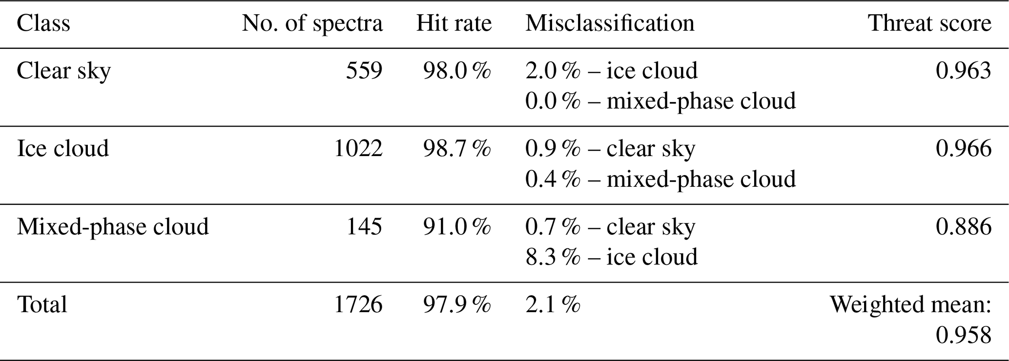
Table 4CIC classification results for the whole REFIR-PAD spectra dataset (2012–2015) and for single years. The associated uncertainties are computed using Eq. (15). Mean air temperatures at surface level for the entire period and for each year are also reported. The last row refers to mean air temperatures at surface level computed for the months from November to March (warm season).
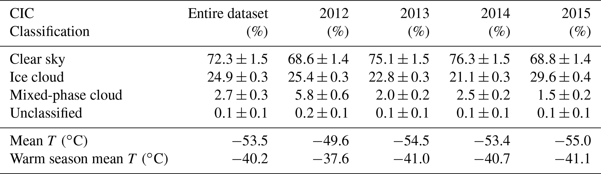
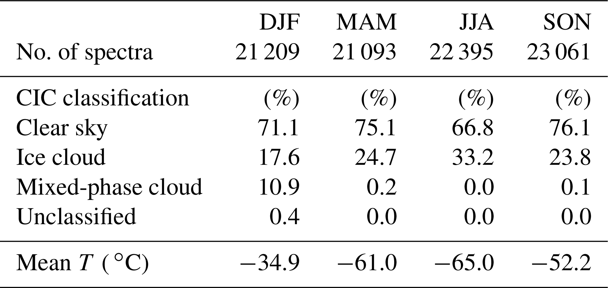
Table 5Mean seasonal occurrences of clear sky, ice clouds, and mixed-phase clouds at Concordia Station. Mean surface air temperatures are reported for each season.
4.1 Sky classification: 4-year averages and inter-annual variability
A total of 87 960 REFIR-PAD spectra are analyzed from the dataset spanning over the time range 2012–2015. From this set, only 202 spectra (see Table 2) are used for training the CIC algorithm, and the other 87 758 are ingested by the CIC to evaluate the cloud occurrence over Concordia Station. The classification results are shown in Table 4 as percentages for clear sky, ice clouds, mixed-phase clouds, and unclassified spectra. The entire dataset and individual year classifications are presented as well as the estimated percentage uncertainties (see Eq. 15). On average, the clear sky is detected in almost 72 % of the cases, with ice cloud occurrence of about 25 % and mixed-phase cloud occurrence of less than 3 %. The inter-annual variability in total cloud occurrence in the Antarctic Plateau, the sum of ice and mixed-phase clouds, spans between about 23 % and 31 %. This percentage interval is in accordance with the observations from Adhikari et al. (2012), who analyzed data from CloudSat and CALIPSO between 2006 and 2010 and reported percentages spanning between 20 %–30 %. From our analysis the cloudiest year in the 2012–2015 period is 2012, with a value of 31.2 %. This is almost identical to what we observed in 2015 (cloud occurrence is 31.1 % in this case), with the difference being that in 2012 there was a significantly larger fraction of mixed-phase clouds than in 2015 (5.8 % and 1.5 %, respectively).
Mean temperatures at the surface level for the entire dataset and for each single year are also reported in Table 4. Temperatures are measured every hour at Concordia Station and are linearly interpolated in time to be associated with the REFIR-PAD measurements and the corresponding CIC classifications. The last row of Table 4 provides information only for the months of the warm macro-season from November to March. The results suggest a positive correlation between mean air temperatures at surface level in the warm macro-season and the occurrence of mixed-phase clouds. Note that mixed-phase clouds are present only for months from November to March. The temperature and mixed-phase cloud correlation could indicate that warm temperatures are favorable for mixed-phase cloud formation or that the presence of warm liquid clouds implies a stronger cloud forcing at the surface and, consequently, an increase in the temperature values near the ground. Another favorable condition for liquid cloud formation consists of the advection of air from warmer and more humid regions such as the Ross Sea and Southern Ocean. Ice clouds are observed during the entire year. In contrast with mixed-phase clouds, their occurrence does not seem correlated to the mean air temperature at the surface. Note that the maximum occurrence of ice clouds is observed during the year 2015, which had the lowest mean value of surface air temperature in the 4-year time range.
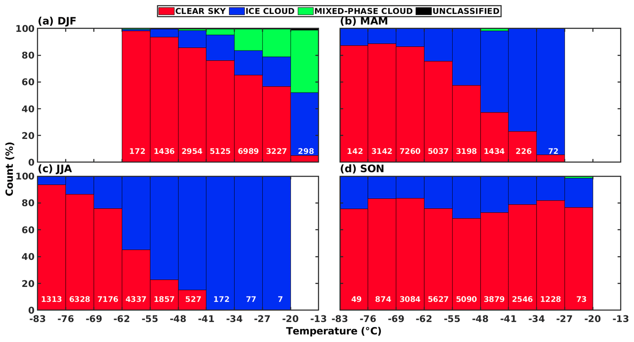
Figure 8Histograms of the seasonal occurrence of the analyzed sky conditions as a function of the surface air temperature. (a) DJF – summer, (b) MAM – autumn, (c) JJA – winter, and (d) SON – spring. The number of observations for each 7 ∘C bin is reported at the base of each histogram.
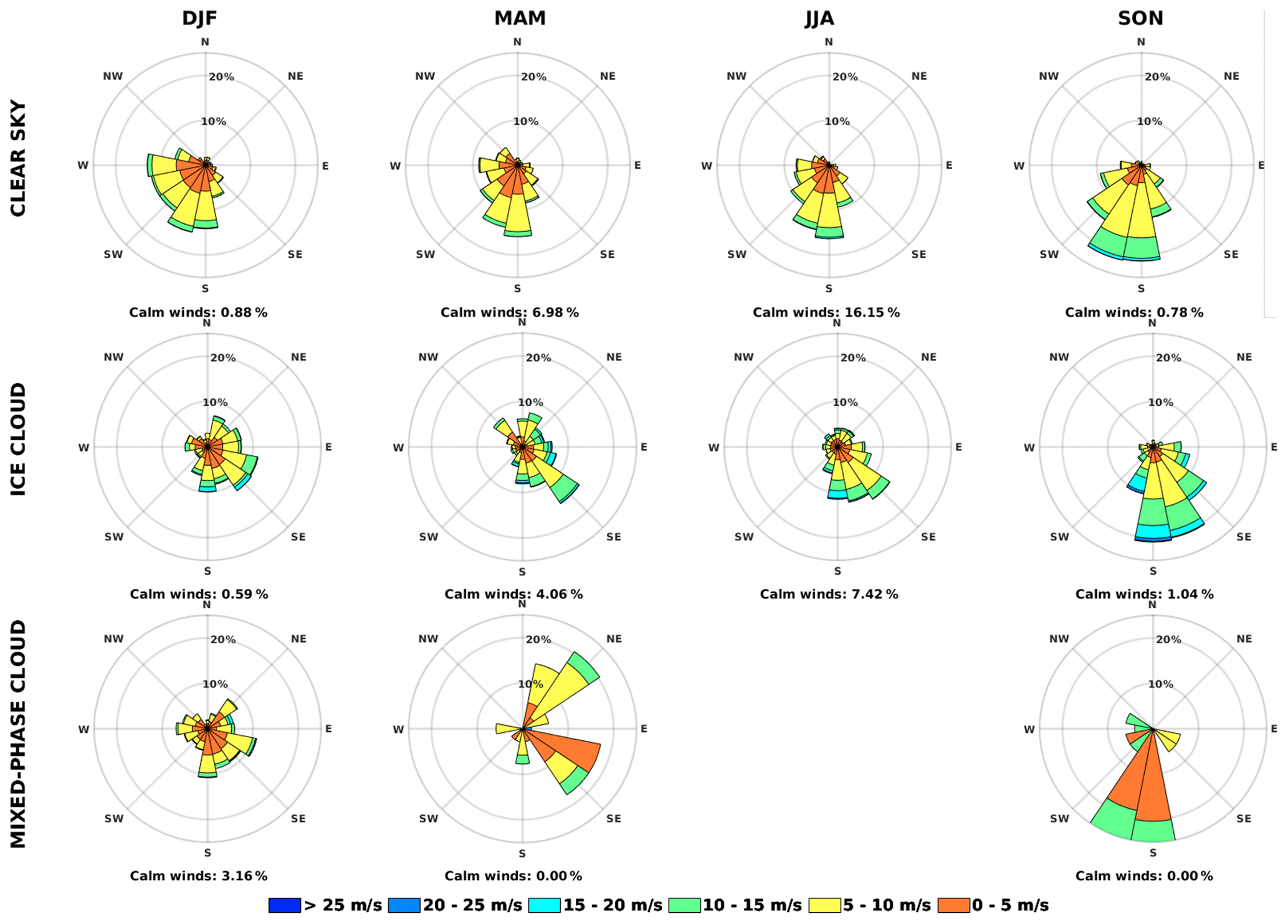
Figure 9Wind roses at Concordia Station for the four seasons (DJF, MAM, JJA, and SON) of the period 2012–2015. Clear-sky, ice cloud, and mixed-phase cloud conditions are split into separate rows.
4.2 Seasonal clear-sky and cloud occurrence
Seasonal averages of cloud occurrence are computed for the entire dataset and presented in Table 5. The table also reports the number of spectra observed in each season, which show that the data are homogeneously distributed over the course of the year, and the mean air temperatures. The mean total cloud occurrence varies from the minimum value of 23.9 % detected in spring (SON) to the maximum value of 33.2 % in the cold winter season (JJA). The dominant cloud occurrence and thermodynamic phase is ice. During the austral summer, the occurrence of ice clouds is the smallest. However, for the same season, the occurrence of mixed-phase clouds reaches its maximum over Concordia Station (10.9 %). It is interesting that during summer, more than one-third of the clouds over Concordia are of the mixed-phase type. The occurrence of mixed-phase clouds in summer is in line with the analysis performed by Listowski et al. (2019), who analyzed DARDAR data (Delanoë and Hogan, 2010; Ceccaldi et al., 2013) based on combined observations from CloudSat and CALIPSO satellites in the period 2007–2010. The same authors, by performing a visual analysis of the geographical distribution of the clouds containing liquid water particles, estimate that during the other seasons (MAM, JJA, and SON), the occurrence of mixed-phase clouds is close to 0 % in the region around Concordia Station.
Seasonal occurrences for each class are analyzed in combination with meteorological parameters encountered during the corresponding REFIR-PAD measurements. In Fig. 8, the percentage distribution of each class seasonal occurrence is reported as a function of the air surface temperature, with histogram binning of 7 ∘C. The same color code that was used previously is adopted here: clear sky in red, ice clouds in blue, and mixed-phase clouds in green. The number of REFIR-PAD measurements for each bin is reported at the base of the histograms. Over the 4 years, the surface air temperature (corresponding to REFIR-PAD measurements) varies between a minimum of and a maximum of . With the exception of the spring season (SON; lower-right panel of Fig. 8), the results show that the detected cloudy-sky occurrence increases (clear skies decrease) as surface air temperature increases. This holds for both ice and mixed-phase clouds. In the winter season (JJA; lower-left panel of Fig. 8), for surface air temperature larger than the CIC identifies only ice cloud conditions. Note that the winter and spring seasons have the largest variation in the air surface temperatures. In the winter season, extremely low temperatures (below ) are very frequent and result from the lack of insolation, the dry atmospheric conditions, and the absence of clouds. In the same season, higher surface temperatures are measured mainly when clouds are present. The downwelling longwave radiation from cloud layers contributes to the surface radiative forcing and mitigates the temperature of the cold season. Over the 4-year period the average winter surface temperature in clear-sky conditions is , while in the presence of ice clouds it is .
A similar analysis is performed by relating clear- and cloudy-sky occurrences to measurements of surface relative humidity and surface pressure. Results (not shown here) indicate that the highest values of relative humidity tend to occur with the highest percentage of clouds for all the seasons except spring. The highest mean values of surface pressure in the summer season tend to occur with the highest percentages of mixed-phase clouds (not shown). Unclassified spectra are obtained only in the summer season and correspond to very high values of surface pressure, air temperature, and relative humidity.
Surface wind measurements are also analyzed and related to CIC classification results for each season. The values of wind speed and direction closest in time to the REFIR-PAD measurements are used. Wind roses are built considering the bias correction methodology proposed by Droppo and Napier (2008), which indicates the necessity of weighting the contribution of each direction to correctly represent them in the wind roses.
In Fig. 9, the wind roses for each season and class are shown. Clear-sky cases correspond to about 70 % of all occurrences in all seasons and are associated with a surface level wind that blows predominantly from the south and southwest. Higher wind intensities are found in springtime. An additional wind component from the west is observed in summer but is negligible in the other seasons. When ice clouds are present, the dominant surface wind direction is from the southeast, and the wind intensity is larger than in clear-sky conditions on average (7.7 m s−1 versus 6.1 m s−1). Note that non-negligible occurrences of surface wind from the northeast are observed only when mixed-phase clouds are detected, especially during the fall (MAM) season. This component overlaps with the dominant southeast wind component found in both summer and autumn. The wind rose for mixed-phase clouds in the spring season (SON) is reported for completeness but is affected by the very few number of cases detected. Even if very preliminary, the analysis of the surface wind direction for different sky conditions highlights some correlations between the wind component and the clear-sky or cloud occurrence. Note (see back to Fig. 1) that south and west directions at Concordia Station point to the inner Antarctic Plateau, where the drier air is supposedly found. Otherwise, the southeast and east directions are towards the Ross Sea and the Southern Ocean, which are characterized by warmer and more humid air. The correlations are far from being conclusive since the upper level winds and the back trajectories of the air masses have not been analyzed yet.
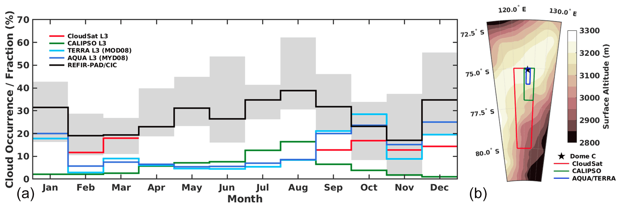
Figure 10(a) Percentage fraction of CIC monthly mean cloud occurrence (in black) compared with the CloudSat L3 product (red line), CALIPSO L3 product (green line), MODIS TERRA L3 product – MOD08 (light-blue line), and MODIS AQUA L3 product – MYD08 (blue line). The shaded gray area indicates the minimum and maximum CIC monthly values in the interval 2012–2015. (b) Location of the Dome Concordia base and extension of the grid sector for CloudSat, CALIPSO, and AQUA/TERRA MODIS L3 data. Surface elevation above mean sea level is also reported.
4.3 Monthly mean cloud occurrence: comparison with satellite data
CIC monthly mean cloud percentages (including ice and mixed-phase) for the period 2012–2015 are shown in Fig. 10 (left panel). The black curve corresponds to the 4-year monthly average cloud occurrence, and the shaded gray area indicates the minimum and maximum CIC monthly values. The lowest average value is found in November (17 %), while higher occurrences are observed during the winter months. The peak is located in August, with an average value of 39 %. For the same month, the inter-annual variability is quite large, as indicated by the extent of the gray area. As examples, in August the monthly mean values span from 31 % to 62 %, which is the highest derived occurrence, and in November from 1 % (lowest registered value) to 37 %.
Monthly mean cloud occurrences and fractions derived from level 3 (L3) satellite products are also reported in the left panel of Fig. 10 for the same period of time. The comparison has a twofold objective: (a) to assess if the results obtained locally from the CIC/REFIR-PAD synergy can be representative of the widespread region characterizing the Antarctic Plateau and (b) to estimate the differences among the cloud occurrences and fractions derived from L3 satellite products around the Concordia area. According to the WMO1, the L3 satellite products are composed of variables mapped on uniform space–time grid scales and are constructed to provide completeness and consistency for the anticipated users. These product types are frequently used to perform climate analysis and model evaluation (e.g., Stubenrauch et al., 2013; Webb et al., 2017). The assessment of their accuracy can be particularly challenging, especially in remote regions such as the Antarctic Plateau, due to the scarcity of ground-based stations that are available for product validation campaigns. For the present study, we only refer to monthly mean L3 satellite products, and the comparison with CIC results is performed only in the context of the objectives described above. A validation (that is outside the scope of the present research) should be, eventually, performed on level 2 collocated satellite products to minimize the bias due to different footprint sizes that can be otherwise very large when accounting for gridded L3 products. In practice, different datasets present specific strengths and limitations that are briefly described below.
The L3 products used in this work are derived from passive radiometric observations performed by the Moderate Resolution Imaging Spectroradiometer (MODIS) on board the TERRA and the AQUA satellite platforms, by the CALIOP on board the CALIPSO satellite, and by the CPR on board CloudSat satellite. For MODIS L3 products, the occurrence by cloud type is not available, and the cloud fraction is used. This variable is computed as the ratio between the cloud-covered pixels and the total number of pixels observed by both satellite platforms each month and is mapped in a global grid of 1∘ of latitude and longitude, which corresponds to an area of about 3000 km2 in the region of Concordia Station. In the right panel of Fig. 10 the boundary of the area which refers to the considered MODIS L3 gridded product is reported in blue. In the same panel the location of the Concordia base is indicated as a black star. The MODIS L3 products used in this study are the MYD08 and MOD08.
They are derived from each MODIS sensor on platforms separately (MYD08 for AQUA and MOD08 for TERRA; MODIS Atmosphere Science Team, 2017). The MOD08 and MYD08 L3 products are based on a cloud mask which exploits infrared and visible bands. When in the absence of solar illumination only the infrared bands are used. The monthly mean cloud fraction from the MODIS sensor is shown in Fig. 10 (light-blue and blue line for MODIS TERRA and AQUA L3 products, respectively).
In contrast to MODIS, the CALIOP and the CPR active sensors detect the cloud occurrence within vertical profiles. The L3 product from these sensors is a volume cloud occurrence, which considers the number of cloud observations along the vertical profiles that are mapped monthly on a regular grid. The CALIOP L3 product (CAL_LID_L3_Cloud_Occurrence-Standard-V1-00; Winker, 2018) is built on a grid map of 2.5∘ of longitude and 2.0∘ of latitude, which corresponds to an area of about 15 000 km2 in the region surrounding Concordia Station and is indicated by a green line in the right panel of Fig. 10. The L3 product from CloudSat (3S-RMCP; Haynes, 2019) is available in a grid of of latitude and longitude that covers an extended area of about 75 000 km2 around Concordia Station, identified by the red line in the right panel of Fig. 10. CloudSat results are reported in red in the left panel of Fig. 10. From the year 2011, the CPR on CloudSat collected data only in daylight hours due to a battery anomaly, so there is no record of cloud occurrence from CloudSat from April to August.
For each one of the MODIS, CALIOP and CPR sensors, the grid point that includes Concordia Station is used to retrieve the monthly L3 satellite product. Monthly time series of the cloud fractions, in the case of MODIS data, and of cloud occurrences, in the case of CALIOP and CPR observations, are computed for the period 2012–2015. Results are compared with the cloud occurrence derived by the CIC algorithm over Concordia Station (left panel of Fig. 10). Since the L3 products of the three sensors refer to multiple extent areas of observations (of the order of tens of thousands of square kilometers), some differences are expected not only between the ground-based measurements analyzed by CIC but also among the mean values of the L3 satellite products. In particular, we note that the gridded L3 products from CALIPSO and CloudSat refer to areas characterized by important variations in surface altitude with possible consequences for cloud formation and occurrence.
In the presence of solar illumination, the lowest cloud occurrence values are those derived from CALIOP products, as shown in green in the left panel of Fig. 10. Despite the very low values, CALIOP is able to identify the maximum in cloud occurrence during the austral winter (specifically August) also detected by the CIC algorithm applied to the REFIR-PAD data. In April through August the MODIS MYD08 and MOD08 products provide very low values of cloud fraction, likely due to the low efficiency of the cloud mask algorithm based on infrared bands only.
From November to March (the warm season), the CIC cloud occurrence is comparable to that found by MODIS and the CPR sensors. Nevertheless, a higher percentage of cloudiness is found by the CIC algorithm with respect to the CPR. The main reasons for such differences are likely due to (1) the high CIC sensitivity to the optically thin ice clouds, which are often present in the Antarctic Plateau (Maestri et al., 2019a) and missed by radar measurements (Henderson et al., 2013; L'Ecuyer et al., 2008); (2) the extension of the gridded area of the CPR L3 product that encompasses regions with surface elevations spanning up to 0.4 km in altitude and which might not be representative of the Dome C conditions; and (3) the CPR coarse vertical resolution (0.5 km), which might be the cause of undetected clouds near the surface (Chan and Comiso, 2011).

Figure 11Hourly mean cloud occurrence of clear sky (red lines), ice clouds (blue lines), and mixed-phase clouds (green line). Unclassified spectra are in black and total cloud occurrence in magenta. Percentages of occurrence are provided for each season: (a) DJF, (b) MAM, (c) JJA, and (d) SON. The top of the atmosphere hourly mean insolation is also reported in Wm−2 (dashed black line), referring to values reported on the right ordinate axis. Local time is UTC+8.
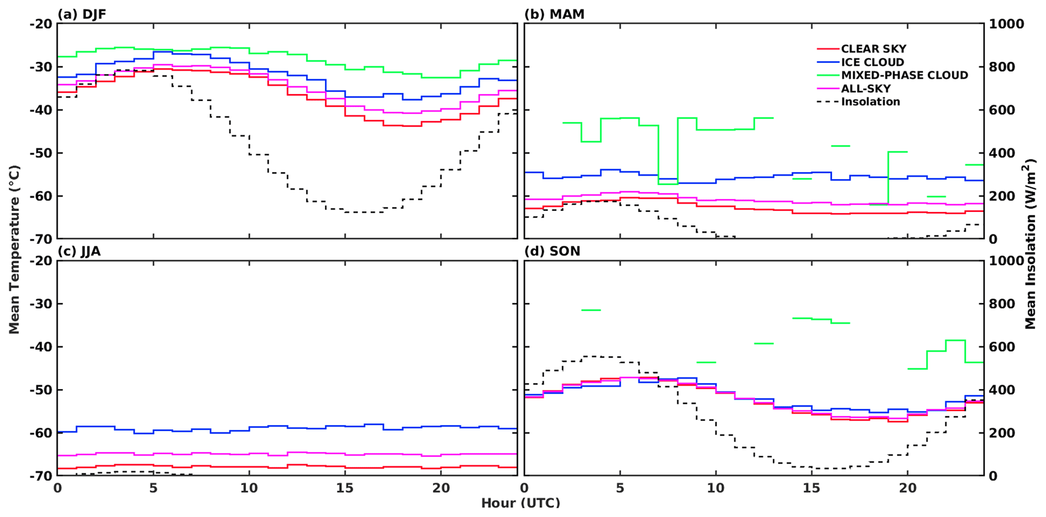
Figure 12Hourly mean surface air temperature, according to the sky condition: clear sky (red line), ice clouds (blue line), mixed-phase clouds (green line), and all sky (magenta line). The temperature is reported according to the season: (a) DJF, (b) MAM, (c) JJA, and (d) SON. The top-of-the-atmosphere hourly mean insolation is also reported in Wm−2 (dashed black line), and values are indicated by the ordinate axis on the right. Local time is UTC+8.
4.4 Diurnal variability in cloud occurrence
The almost continuous REFIR-PAD measurements during the 4-year period provide an opportunity to investigate an hourly mean cloud occurrence. The time collocation of each CIC classification is obtained by associating each spectra with the hourly time of observation. For instance, observations performed between 01:00:00 and 01:59:59 UTC are associated with the time 01:00:00 UTC. For each hour, the percentage of occurrence of each class is computed, and results are reported in Fig. 11. Results are also presented as seasonal means.
In the austral summer (upper left panel of Fig. 11), a diurnal cycle is observed and related to the hourly mean insolation, also reported in the same figure with a dotted black curve. The clear-sky occurrence is characterized by a maximum value of about 78 % at around 05:00 UTC (13:00 LT). This maximum is very close in time to the maximum of insolation for the same period of the year. In the summer season, the highest percentage of occurrence of cloudiness (about 36 %) is obtained during nighttime hours that correspond to the coldest time of the day. For the other seasons, a clear diurnal cycle of the percentage occurrences is not observed. Note that for the fall and spring seasons the daily variation in the insolation is much less intense than for austral summer, and in winter it is almost null. In the austral autumn (MAM; panel b) and spring (SON; panel d) seasons the clouds are almost entirely composed of ice since mixed-phase clouds are very rare. In the austral winter (JJA; panel c) the insolation is close to zero, and the ice cloud occurrence reaches its seasonal maximum.
In Fig. 12, the hourly mean surface air temperature is plotted for the four seasons for clear sky, ice clouds, and mixed-phase clouds. The hourly mean temperatures are also presented for all-sky conditions (magenta line) and the hourly mean top-of-the-atmosphere insolation (dashed black curve). The all-sky hourly mean air surface temperature is driven by the diurnal cycle of insolation in summer and spring: a lag of about 2 h is observed between the maximum in insolation and the maximum in temperature. The all-sky surface air temperature has a 11.2 ∘C amplitude in summer, when the top-of-the-atmosphere diurnal cycle of insolation is the largest. This amplitude decreases as the insolation cycle becomes weaker, and it is almost null in winter.
The surface mean air temperature is higher in cloudy-sky conditions (ice cloud or mixed-phase cloud) than for clear sky at all hours of the day, suggesting a positive cloud forcing at the surface level. Mean values of surface air temperature are higher in the presence of mixed-phase clouds than ice clouds at all times of the day. Observations of mixed-phase clouds (green curves) are rare in autumn and spring, and the data do not cover the full day in these seasons. Note that when mixed-phase clouds are present, the daily thermal amplitude is smoothed with respect to the other sky conditions. The main reason for this could be related to the relatively larger optical thickness of liquid water clouds with respect to ice clouds (Di Natale et al., 2020), which implies a decrease in surface insolation and thus a dampening of the diurnal cycle of surface temperature due to the reduced solar warming. The hourly mean surface temperature is larger when ice clouds are present than in clear-sky conditions. This difference is on average larger in winter (about 9 ∘C) and autumn (about 7 ∘C), diminishes in summer (about 4 ∘C), and becomes very small in spring (about 1 ∘C). The cause of this low value needs further investigation. Possible explanations could be related to the optical thickness and position of the clouds and/or related to the circulation of the air in the area that is not accounted for in this analysis. For the spring and summer seasons, where the insolation diurnal cycle is larger, the surface temperature difference is greater between the clear-sky and ice cloud conditions for low insolation but decreases for higher insolation.
High-spectral-resolution downwelling radiances at far-infrared (FIR) and mid-infrared (MIR) wavelengths are measured by the REFIR-PAD spectroradiometer located at Dome C on the Antarctic Plateau between 2012–2015. The spectral radiance measurements are, for the first time, ingested by an automatic machine learning algorithm called CIC to perform single spectrum classifications. CIC is developed to identify high-spectral-resolution observations and, in the case of a cloudy scene, to perform a classification. The algorithm is computationally very fast and only requires a limited number of spectra as a training set, which makes it very flexible, efficient, user-friendly, and easy to adapt to different types of sensors. For this study, the algorithm is arranged and optimized to classify a REFIR-PAD spectrum as being a clear sky, ice cloud, or mixed-phase cloud. In the Dome C region, mixed-phase clouds are usually characterized by at least one layer of water in the liquid phase. Typically, an ice layer close to the cloud top and weak precipitation of ice crystals are also observed.
While an accurate description of clear and cloud properties is quite difficult in the Antarctic from passive measurements alone, our analysis of the REFIR-PAD data is greatly enhanced through coincident active measurements of atmospheric backscattering and depolarization ratio profiles measured by a lidar system that is temporally co-located with the REFIR-PAD radiance measurements. The coincident lidar and REFIR-PAD measurements are used to obtain accurate training sets for the CIC algorithm. The training sets are formed by using a total of 202 spectra that are sufficient to characterize the large variability in the atmospheric conditions in the Antarctic Plateau region. An analysis of the lidar data and atmospheric vertical profiles of temperature and humidity, obtained from radiosondes launched every day at Concordia Station, is used to separate the training sets into two macro seasons. The first is named the warm season and ranges between November and March. Three training sets, defining three different classes of spectra, are considered for the warm season: clear sky, ice cloud, and mixed-phase cloud. The second macro-season is named the cold season and corresponds to the period from April to October. For the cold season, only two classes are considered (clear sky and ice cloud) since layers in the liquid phase are rarely observed during this period due to the extremely cold atmospheric temperatures.
A number of 1726 lidar co-located REFIR-PAD measurements are then used to select a test set of spectra, previously classified according to the lidar backscatter and depolarization ratio vertical profiles. This sample is used to test the algorithm performance, to estimate the CIC classification uncertainty, and to optimize the classification results for each class. For the optimization process, the CIC algorithm is applied to classify the test set by considering different spectral intervals. A weighted threat score (ThS) is used to select the optimal spectral range for the classification. Results show that the spectral interval 380–1000 cm−1 provides the best score due to the experimental and observational conditions. This result highlights the fundamental role of the FIR part of the spectrum to improve the process of clear-sky and cloud identification and cloud type classification in the Antarctic.
The optimized CIC algorithm is then applied to the entire REFIR-PAD dataset from 2012 to 2015 consisting of 87 758 spectra. On average, clear-sky conditions are detected in almost 72 % of the cases with an associated uncertainty of the order of 1.5 %. The ice cloud occurrence is about 25 %, and the mixed-phase clouds are identified in less than 3 % of the observations. The uncertainty is 0.3 % in cloudy conditions. The cloud occurrence over the Antarctic Concordia Station is analyzed at different temporal scales: inter-annual, seasonal, monthly, and daily variability. The inter-annual variability in total cloud occurrence spans between about 23 % and 31 %. A positive correlation is observed between mean air temperatures at surface level, in the warm macro-season, and the occurrence of mixed-phase clouds. This result suggests that (a) warm temperatures due to meteorological conditions (including warm and humid air advection) are favorable for the mixed-phase cloud formation or that (b) the occurrence of warm cloud layers enhances the cloud radiative forcing at the surface with a consequent increase in the surface temperature. Further work is needed for a better identification of the key atmospheric conditions and understanding of the physical processes driving to mixed-phase cloud formation in the Antarctic.
Seasonal analysis indicates that the mean total cloud occurrence varies from 23.9 % in the spring (SON) to 33.2 % in the cold winter season (JJA), when only ice clouds are present. In fact, most of the mixed-phase clouds are observed in the summer season, where they amount to more than one-third of the total clouds over Concordia Station. The seasonal scene classification is analyzed in accordance with meteorological parameters. Results show that the highest values of surface air temperature (and relative humidity) are found corresponding to the highest amounts of cloud for the summer, fall, and winter seasons; in the spring this relationship is minimal. The influence of the longwave radiative forcing of ice clouds on surface temperature is most observed in the winter months, where the insolation is negligible. For this season, the mean surface temperature is about in clear sky and in the presence of clouds. Furthermore, surface level winds from the south and southwest are more frequently observed in clear-sky conditions, while in the presence of ice clouds the surface wind is primarily from the southeast. When mixed-phase clouds are identified, surface winds from the eastern quadrant are more frequent. The mean wind intensity is about 2 m s−1 higher in the presence of ice clouds than in clear atmospheric conditions.
CIC monthly mean cloud occurrences show, on average, a maximum in August and a minimum in November. The inter-annual variability in monthly mean cloud occurrences can be very high. Noteworthy is the November case that registers a cloud occurrence variation spanning from 0 % to 40 % among the 4 years of analysis.
The monthly mean data are compared with Level-3 satellite products derived from the MODIS (passive imager), CALIOP (lidar), and CPR (radar) sensors and referring to gridded areas covering the Dome C location. The discussion of the results accounts for the different measurement techniques and sensitivity to cloud layers and for the large differences in the dimensions of the gridded areas considered.
Some differences are observed among the analyzed products. In periods of higher insolation the lowest values of monthly cloud occurrence are those derived from CALIOP. Despite the low scores, CALIOP data indicate that the maximum cloud occurrence in winter (August) is similar to what is derived by the CIC algorithm. For the months from November to March, which correspond to the warm season, the CIC cloud occurrence is larger but comparable to what is found by the MODIS (whose algorithm benefits from the shortwave reflected radiation) and CPR sensors. The higher values detected by the CIC are probably due to its greater sensitivity to thin cirrus clouds and to its ability to detect cloud layers near the surface. The added value of both the local and continuous measurements is demonstrated. The CIC results, by exploitation of REFIR-PAD FIR and MIR spectral data available at all times during the year, provide a continuous record of cloud occurrence with excellent classification scores.
Finally, an hourly cloud occurrence analysis is performed that shows the presence of a diurnal cycle with a maximum of about 36 % and a minimum of 22 % during the austral summer that follows the hourly mean insolation. The highest cloud occurrences are observed during nighttime hours. Conversely, the season maximum of clear-sky occurrence is observed corresponding to the local noontime. For all the other seasons, diurnal cycles are not observed for either cloud or clear-sky conditions. An analysis between the daily sky condition and the surface mean air temperature reveals higher surface temperatures in cloudy-sky conditions, especially for mixed-phase clouds, than in clear sky for all the seasons and hours of the day. In summer, the mean surface air temperature in the presence of clouds is on average 5 ∘C warmer than in clear sky. This difference is larger during the night but smaller during the day, probably due to the amount of insolation. The same effect, although smaller, is observed in fall and spring due to a weaker insolation cycle. In the winter, where the insolation is almost null, the difference between surface air temperature measured in cloudy sky and clear sky is constant at about 9 ∘C throughout the day, which quantifies the effect of the longwave radiative forcing of the Antarctic winter clouds.
The results of this work provide a basis for understanding of cloud occurrence at different timescales on the Antarctic Plateau, where cloud identification and classification from satellites are challenging. The obtained results provide a useful benchmark for satellite and model product comparisons and open the path to new investigations.
The use of FIR and MIR high-spectral-resolution radiances for the cloud identification and classification contributes to the preparatory studies for the Far-infrared Outgoing Radiation Understanding and Monitoring (FORUM) mission. FORUM was recently selected as the ESA's 9th Earth Explorer mission and is scheduled for launch in 2026.
| ϵTS | Training set eigenvector matrix |
| ϵETS | Extended training set eigenvector matrix |
| a.m.s.l. | Above mean sea level |
| AWS | Automatic weather station |
| BT | Brightness temperature |
| CIC | Cloud identification and classification |
| CoMPASs | Concordia Multi-Process Atmospheric Studies |
| CALIOP | Cloud–Aerosol Lidar with Orthogonal Polarization |
| CALIPSO | Cloud–Aerosol Lidar and Infrared Pathfinder Satellite Observation |
| CPR | Cloud Profiling Radar |
| ERB | Earth's radiation budget |
| ETS | Extended training set |
| FIR | Far infrared |
| FN | False negative |
| FORUM | Far-infrared Outgoing Radiation Understanding and Monitoring |
| FP | False positive |
| IND | Indicator function |
| IPEV | French Polar Institute Paul-Émile Victor (abbreviation from the French institute named “Institut Polaire Français Paul Émile Victor”) |
| Lidar | Light detection and ranging |
| MIR | Mid-infrared |
| MODIS | Moderate Resolution Imaging Spectroradiometer |
| PCA | Principal component analysis |
| PNRA | Italian National Program for Research in Antarctica (abbreviation from the Italian program named “Programma Nazionale di Ricerche in Antartide”) |
| PRANA | Radiative Properties of Water Vapor and Clouds in Antarctica (abbreviation from the Italian project named “Proprietà Radiative dell'Atmosfera e delle Nubi in Antartide”) |
| REFIR-PAD | Radiation Explorer in the Far Infrared – Prototype for Applications and Development |
| SI | Similarity index |
| SID | Similarity index difference |
| ThS | Threat score |
| TN | True negative |
| TP | True positive |
| TS | Training set |
| WMO | World Meteorological Organization |
The combined AQUA/TERRA L3 products are accessible at https://ladsweb.modaps.eosdis.nasa.gov/archive/allData/61/MCD06COSP_M3_MODIS/ (last access: 24 August 2021). The AQUA L3 products are accessible at https://ladsweb.modaps.eosdis.nasa.gov/archive/allData/61/MYD08_M3/ (last access: 24 August 2021). The TERRA L3 products are accessible at https://ladsweb.modaps.eosdis.nasa.gov/archive/allData/61/MOD08_M3/ (last access: 24 August 2021). The CALIPSO L3 data are accessible at https://opendap.larc.nasa.gov/opendap/CALIPSO/LID_L3_Cloud_Occurrence-Standard-V1-00/ (last access: 24 August 2021). The CloudSat L3 data are reachable from http://www.cloudsat.cira.colostate.edu/data-products/level-aux/3f-rmcp-3s-rmcp?term=105 (last access: 24 August 2021). The Antarctic lidar data are reachable at http://lidarmax.altervista.org/englidar/Antarctic%20LIDAR.php (last access: 24 August 2021). Radiosondes and meteorological data are available at http://www.climantartide.it (last access: 24 August 2021). REFIR-PAD radiances can be acquired from http://refir.fi.ino.it/refir-pad-domeC.php (last access: 24 August 2021).
The CIC source code version used in the present paper is available on request to the corresponding author.
TM was responsible for conceptualization. WC, DM, and TM designed the methodology, prepared and evaluated the data, and performed the cloud classification. WC, DM, MM, and TM evaluated the results. WC downloaded and prepared the meteorological and satellite data. GDN, GB, LP, and MDG prepared and evaluated the REFIR-PAD and lidar data. All authors revised the manuscript.
The authors declare that they have no conflict of interest.
Publisher's note: Copernicus Publications remains neutral with regard to jurisdictional claims in published maps and institutional affiliations.
The present work is in preparation of the FORUM mission. FORUM-related studies are supported by projects of the Italian Space Agency (ASI) and of the European Space Agency (ESA). We thank the Italian PNRA (Programma Nazionale di Ricerche in Antartide) and the Institut Polaire Français Paul Émile Victor (IPEV). More specifically, data were obtained as a part of the subprojects PRANA (Proprietà Radiative dell'Atmosfera e delle Nubi in Antartide), COMPASS (Concordia Multi-Process Atmospheric Studies), FIRCLOUDS (Far Infrared Radiative Closure Experiment For Antarctic Clouds), and DOCTOR (Dome-C Tropospheric Observer). The authors acknowledge the Antarctic Meteo-Climatological Observatory at Concordia for the meteorological data availability as part of the IPEV/PNRA project “Routine Meteorological Observation at Station Concordia”. We thank the CALIPSO team and the Atmospheric Science Data Center at NASA Langley Research Center for archiving and hosting CALIPSO data. We thank the CloudSat team and the CloudSat Data Processing Center for archiving and hosting CloudSat data. We thank also the MODIS team and the Level 1 and Atmosphere Archive and Distribution System Distributed Active Archive Center (LAADS DAAC) for making the MODIS data available.
The authors acknowledge the use of computational resources from the parallel computing cluster of the Open Physics Hub (https://site.unibo.it/openphysicshub/en, last access: 14 September 2021) at the Physics and Astronomy Department in Bologna.
This paper was edited by Michael Schulz and reviewed by M. G. Mlynczak, Xianglei Huang, and Bryan A. Baum.
Adhikari, L., Wang, Z., and Deng, M.: Seasonal variations of Antarctic clouds observed by CloudSat and CALIPSO satellites, J. Geophys. Res.-Atmos., 117, D04202, https://doi.org/10.1029/2011jd016719, 2012. a, b, c
Bianchini, G., Castagnoli, F., Di Natale, G., and Palchetti, L.: A Fourier transform spectroradiometer for ground-based remote sensing of the atmospheric downwelling long-wave radiance, Atmos. Meas. Tech., 12, 619–635, https://doi.org/10.5194/amt-12-619-2019, 2019. a
Bromwich, D. H., Nicolas, J. P., Hines, K. M., Kay, J. E., Key, E. L., Lazzara, M. A., Lubin, D., McFarquhar, G. M., Gorodetskaya, I. V., Grosvenor, D. P., Lachlan-Cope, T., and van Lipzig, N. P. M.: Tropospheric clouds in Antarctica, Rev. Geophys., 50, RG1004, https://doi.org/10.1029/2011rg000363, 2012. a, b, c, d
Ceccaldi, M., Delanoë, J., Hogan, R. J., Pounder, N. L., Protat, A., and Pelon, J.: From CloudSat-CALIPSO to EarthCare: Evolution of the DARDAR cloud classification and its comparison to airborne radar-lidar observations, J. Geophys. Res.-Atmos., 118, 7962–7981, https://doi.org/10.1002/jgrd.50579, 2013. a
Chan, M. A. and Comiso, J. C.: Cloud features detected by MODIS but not by CloudSat and CALIOP, Geophys. Res. Lett., 38, L24813, https://doi.org/10.1029/2011gl050063, 2011. a, b
Chan, M. A. and Comiso, J. C.: Arctic Cloud Characteristics as Derived from MODIS, CALIPSO, and CloudSat, J. Climate, 26, 3285–3306, https://doi.org/10.1175/jcli-d-12-00204.1, 2013. a
Cox, C. J., Turner, D. D., Rowe, P. M., Shupe, M. D., and Walden, V. P.: Cloud Microphysical Properties Retrieved from Downwelling Infrared Radiance Measurements Made at Eureka, Nunavut, Canada (2006–09), J. Appl. Meteorol. Clim., 53, 772–791, https://doi.org/10.1175/jamc-d-13-0113.1, 2014. a
Delanoë, J. and Hogan, R. J.: Combined CloudSat-CALIPSO-MODIS retrievals of the properties of ice clouds, J. Geophys. Res., 115, D00H29, https://doi.org/10.1029/2009jd012346, 2010. a
Di Natale, G., Palchetti, L., Bianchini, G., and Del Guasta, M.: Simultaneous retrieval of water vapour, temperature and cirrus clouds properties from measurements of far infrared spectral radiance over the Antarctic Plateau, Atmos. Meas. Tech., 10, 825–837, https://doi.org/10.5194/amt-10-825-2017, 2017. a
Di Natale, G., Bianchini, G., Del Guasta, M., Ridolfi, M., Maestri, T., Cossich, W., Magurno, D., and Palchetti, L.: Characterization of the Far Infrared Properties and Radiative Forcing of Antarctic Ice and Water Clouds Exploiting the Spectrometer-LiDAR Synergy, Remote Sens.-Basel, 12, 3574, https://doi.org/10.3390/rs12213574, 2020. a, b
Droppo, J. G. and Napier, B. A.: Wind Direction Bias in Generating Wind Roses and Conducting Sector-Based Air Dispersion Modeling, Journal of the Air and Waste Management Association, 58, 913–918, https://doi.org/10.3155/1047-3289.58.7.913, 2008. a
Freudenthaler, V., Homburg, F., and Jäger, H.: Optical parameters of contrails from lidar measurements: Linear depolarization, Geophys. Res. Lett., 23, 3715–3718, https://doi.org/10.1029/96gl03646, 1996. a
Haynes, J.: CloudSat Level 3 RMCP Gridded Data Product, CloudSat [data set], available at: http://www.cloudsat.cira.colostate.edu (last access: 14 September 2021), 2019. a
Henderson, D. S., L'Ecuyer, T., Stephens, G., Partain, P., and Sekiguchi, M.: A Multisensor Perspective on the Radiative Impacts of Clouds and Aerosols, J. Appl. Meteorol. Clim., 52, 853–871, https://doi.org/10.1175/jamc-d-12-025.1, 2013. a
Kiehl, J. T. and Trenberth, K. E.: Earth's annual global mean energy budget, B. Am. Meteorol. Soc., 78, 197–207, 1997. a
King, J. C. and Turner, J.: Antarctic Meteorology and Climatology, Cambridge University Press, https://doi.org/10.1017/cbo9780511524967, 1997. a, b, c
King, M., Kaufman, Y., Menzel, W., and Tanre, D.: Remote sensing of cloud, aerosol, and water vapor properties from the moderate resolution imaging spectrometer (MODIS), IEEE T. Geosci. Remote, 30, 2–27, https://doi.org/10.1109/36.124212, 1992. a
Lachlan-Cope, T.: Antarctic clouds, Polar Research, 29, 150–158, https://doi.org/10.1111/j.1751-8369.2010.00148.x, 2010. a
L'Ecuyer, T. S., Wood, N. B., Haladay, T., Stephens, G. L., and Stackhouse, P. W.: Impact of clouds on atmospheric heating based on the R04 CloudSat fluxes and heating rates data set, J. Geophys. Res., 113, D00A15, https://doi.org/10.1029/2008jd009951, 2008. a
Liou, K.: An introduction to atmospheric radiation, Academic Press, Amsterdam, Boston, 2002. a
Liou, K. and Yang, P.: Light scattering by ice crystals: fundamentals and applications, Cambridge University Press, Cambridge, 2016. a
Listowski, C., Delanoë, J., Kirchgaessner, A., Lachlan-Cope, T., and King, J.: Antarctic clouds, supercooled liquid water and mixed phase, investigated with DARDAR: geographical and seasonal variations, Atmos. Chem. Phys., 19, 6771–6808, https://doi.org/10.5194/acp-19-6771-2019, 2019. a, b, c
Lubin, D., Chen, B., Bromwich, D. H., Somerville, R. C. J., Lee, W.-H., and Hines, K. M.: The Impact of Antarctic Cloud Radiative Properties on a GCM Climate Simulation, J. Climate, 11, 447–462, https://doi.org/10.1175/1520-0442(1998)011<0447:tioacr>2.0.co;2, 1998. a
Lubin, D., Zhang, D., Silber, I., Scott, R. C., Kalogeras, P., Battaglia, A., Bromwich, D. H., Cadeddu, M., Eloranta, E., Fridlind, A., Frossard, A., Hines, K. M., Kneifel, S., Leaitch, W. R., Lin, W., Nicolas, J., Powers, H., Quinn, P. K., Rowe, P., Russell, L. M., Sharma, S., Verlinde, J., and Vogelmann, A. M.: AWARE: The Atmospheric Radiation Measurement (ARM) West Antarctic Radiation Experiment, B. Am. Meteorol. Soc., 101, E1069–E1091, https://doi.org/10.1175/BAMS-D-18-0278.1, 2020. a
Maestri, T., Arosio, C., Rizzi, R., Palchetti, L., Bianchini, G., and Guasta, M. D.: Antarctic Ice Cloud Identification and Properties Using Downwelling Spectral Radiance From 100 to 1, 400 cm−1, J. Geophys. Res.-Atmos., 124, 4761–4781, https://doi.org/10.1029/2018jd029205, 2019a. a, b
Maestri, T., Cossich, W., and Sbrolli, I.: Cloud identification and classification from high spectral resolution data in the far infrared and mid-infrared, Atmos. Meas. Tech., 12, 3521–3540, https://doi.org/10.5194/amt-12-3521-2019, 201b. a, b, c, d, e
Magurno, D., Cossich, W., Maestri, T., Bantges, R., Brindley, H., Fox, S., Harlow, C., Murray, J., Pickering, J., Warwick, L., and Oetjen, H.: Cirrus Cloud Identification from Airborne Far-Infrared and Mid-Infrared Spectra, Remote Sens.-Basel, 12, 2097, https://doi.org/10.3390/rs12132097, 2020. a
Mahesh, A., Walden, V. P., and Warren, S. G.: Ground-Based Infrared Remote Sensing of Cloud Properties over the Antarctic Plateau. Part I: Cloud-Base Heights, J. Appl. Meteorol., 40, 1265–1278, https://doi.org/10.1175/1520-0450(2001)040<1265:gbirso>2.0.co;2, 2001. a
MODIS Atmosphere Science Team: MODIS/Terra and MODIS/Aqua Aerosol Cloud Water Vapor Ozone Monthly L3 Global 1 Deg CMG, NASA Level 1 and Atmosphere Archive and Distribution System (LAADS), Greenbelt, Maryland, USA [data set], https://doi.org/10.5067/MODIS/MOD08_M3.061, 2017. a
Palchetti, L., Bianchini, G., Natale, G. D., and Guasta, M. D.: Far-Infrared Radiative Properties of Water Vapor and Clouds in Antarctica, B. Am. Meteorol. Soc., 96, 1505–1518, https://doi.org/10.1175/bams-d-13-00286.1, 2015. a, b, c, d
Palchetti, L., Di Natale, G., and Bianchini, G.: Remote sensing of cirrus cloud microphysical properties using spectral measurements over the full range of their thermal emission, J. Geophys. Res.-Atmos., 121, 10,804–10,819, https://doi.org/10.1002/2016JD025162, 2016. a
Palchetti, L., Brindley, H., Bantges, R., Buehler, S. A., Camy-Peyret, C., Carli, B., Cortesi, U., Bianco, S. D., Natale, G. D., Dinelli, B. M., Feldman, D., Huang, X. L., C.-Labonnote, L., Libois, Q., Maestri, T., Mlynczak, M. G., Murray, J. E., Oetjen, H., Ridolfi, M., Riese, M., Russell, J., Saunders, R., and Serio, C.: FORUM: Unique Far-Infrared Satellite Observations to Better Understand How Earth Radiates Energy to Space, B. Am. Meteorol. Soc., 101, E2030–E2046, https://doi.org/10.1175/bams-d-19-0322.1, 2020. a
Rathke, C., Fischer, J., Neshyba, S., and Shupe, M.: Improving IR cloud phase determination with 20 microns spectral observations, Geophys. Res. Lett., 29, 50-1–50-4, https://doi.org/10.1029/2001gl014594, 2002. a
Ricaud, P., Del Guasta, M., Bazile, E., Azouz, N., Lupi, A., Durand, P., Attié, J.-L., Veron, D., Guidard, V., and Grigioni, P.: Supercooled liquid water cloud observed, analysed, and modelled at the top of the planetary boundary layer above Dome C, Antarctica, Atmos. Chem. Phys., 20, 4167–4191, https://doi.org/10.5194/acp-20-4167-2020, 2020. a, b, c
Sassen, K.: The Polarization Lidar Technique for Cloud Research: A Review and Current Assessment, B. Am. Meteorol. Soc., 72, 1848–1866, https://doi.org/10.1175/1520-0477(1991)072<1848:tpltfc>2.0.co;2, 1991. a
Sassen, K. and Hsueh, C. Y.: Contrail properties derived from high-resolution polarization lidar studies during SUCCESS, Geophys. Res. Lett., 25, 1165–1168, https://doi.org/10.1029/97gl03503, 1998. a
Silber, I., Verlinde, J., Eloranta, E. W., and Cadeddu, M.: Antarctic Cloud Macrophysical, Thermodynamic Phase, and Atmospheric Inversion Coupling Properties at McMurdo Station: I. Principal Data Processing and Climatology, J. Geophys. Res.-Atmos., 123, 6099–6121, https://doi.org/10.1029/2018jd028279, 2018. a
Stubenrauch, C. J., Rossow, W. B., Kinne, S., Ackerman, S., Cesana, G., Chepfer, H., Girolamo, L. D., Getzewich, B., Guignard, A., Heidinger, A., Maddux, B. C., Menzel, W. P., Minnis, P., Pearl, C., Platnick, S., Poulsen, C., Riedi, J., Sun-Mack, S., Walther, A., Winker, D., Zeng, S., and Zhao, G.: Assessment of Global Cloud Datasets from Satellites: Project and Database Initiated by the GEWEX Radiation Panel, B. Am. Meteorol. Soc., 94, 1031–1049, https://doi.org/10.1175/bams-d-12-00117.1, 2013. a
Town, M. S., Walden, V. P., and Warren, S. G.: Spectral and Broadband Longwave Downwelling Radiative Fluxes, Cloud Radiative Forcing, and Fractional Cloud Cover over the South Pole, J. Climate, 18, 4235–4252, https://doi.org/10.1175/jcli3525.1, 2005. a
Turner, D. D., Knuteson, R. O., Revercomb, H. E., Lo, C., and Dedecker, R. G.: Noise Reduction of Atmospheric Emitted Radiance Interferometer (AERI) Observations Using Principal Component Analysis, J. Atmos. Ocean. Tech., 23, 1223–1238, https://doi.org/10.1175/jtech1906.1, 2006. a
Verlinden, K. L., Thompson, D. W. J., and Stephens, G. L.: The Three-Dimensional Distribution of Clouds over the Southern Hemisphere High Latitudes, J. Climate, 24, 5799–5811, https://doi.org/10.1175/2011jcli3922.1, 2011. a
Walsh, J. E., Bromwich, D. H., Overland, J. E., Serreze, M. C., and Wood, K. R.: 100 years of Progress in Polar Meteorology, Meteor. Mon., 59, 21.1–21.36, https://doi.org/10.1175/amsmonographs-d-18-0003.1, 2018. a
Webb, M. J., Andrews, T., Bodas-Salcedo, A., Bony, S., Bretherton, C. S., Chadwick, R., Chepfer, H., Douville, H., Good, P., Kay, J. E., Klein, S. A., Marchand, R., Medeiros, B., Siebesma, A. P., Skinner, C. B., Stevens, B., Tselioudis, G., Tsushima, Y., and Watanabe, M.: The Cloud Feedback Model Intercomparison Project (CFMIP) contribution to CMIP6, Geosci. Model Dev., 10, 359–384, https://doi.org/10.5194/gmd-10-359-2017, 2017. a
Winker, D.: CALIPSO Lidar Level 3 Cloud Occurrence Data, Standard V1-00, NASA Earthdata [data set], available at: https://asdc.larc.nasa.gov/project/CALIPSO/CAL_LID_L3_Cloud_Occurrence-Standard-V1-00_V1-00 (last access: 14 September 2021), 2018. a
World Meteorological Organization – https://community.wmo.int/activity-areas/wmo-space-programme-wsp/data-products, last access: 14 September 2021.
- Abstract
- Introduction
- Instrumentation and measurements
- Cloud identification and classification algorithm
- Results
- Summary and conclusion
- Appendix A: List of abbreviations
- Data availability
- Code and data availability
- Author contributions
- Competing interests
- Disclaimer
- Acknowledgements
- Review statement
- References