the Creative Commons Attribution 4.0 License.
the Creative Commons Attribution 4.0 License.
 | 06 Sep 2021
Predicting gas–particle partitioning coefficients of atmospheric molecules with machine learning
Emma Lumiaro
Milica Todorović
Theo Kurten
Hanna Vehkamäki
Patrick Rinke
The formation, properties, and lifetime of secondary organic aerosols in the atmosphere are largely determined by gas–particle partitioning coefficients of the participating organic vapours. Since these coefficients are often difficult to measure and to compute, we developed a machine learning model to predict them given molecular structure as input. Our data-driven approach is based on the dataset by Wang et al. (2017), who computed the partitioning coefficients and saturation vapour pressures of 3414 atmospheric oxidation products from the Master Chemical Mechanism using the COSMOtherm programme. We trained a kernel ridge regression (KRR) machine learning model on the saturation vapour pressure (Psat) and on two equilibrium partitioning coefficients: between a water-insoluble organic matter phase and the gas phase (KWIOM/G) and between an infinitely dilute solution with pure water and the gas phase (KW/G). For the input representation of the atomic structure of each organic molecule to the machine, we tested different descriptors. We find that the many-body tensor representation (MBTR) works best for our application, but the topological fingerprint (TopFP) approach is almost as good and computationally cheaper to evaluate. Our best machine learning model (KRR with a Gaussian kernel + MBTR) predicts Psat and KWIOM/G to within 0.3 logarithmic units and KW/G to within 0.4 logarithmic units of the original COSMOtherm calculations. This is equal to or better than the typical accuracy of COSMOtherm predictions compared to experimental data (where available). We then applied our machine learning model to a dataset of 35 383 molecules that we generated based on a carbon-10 backbone functionalized with zero to six carboxyl, carbonyl, or hydroxyl groups to evaluate its performance for polyfunctional compounds with potentially low Psat. The resulting saturation vapour pressure and partitioning coefficient distributions were physico-chemically reasonable, for example, in terms of the average effects of the addition of single functional groups. The volatility predictions for the most highly oxidized compounds were in qualitative agreement with experimentally inferred volatilities of, for example, α-pinene oxidation products with as yet unknown structures but similar elemental compositions.
- Article
(1566 KB) - Full-text XML
- BibTeX
- EndNote


Aerosols in the atmosphere are fine solid or liquid particles (or droplets) suspended in air. They scatter and absorb solar radiation, form cloud droplets in the atmosphere, affect visibility and human health, and are responsible for large uncertainties in the study of climate change (IPCC, 2013). Most aerosol particles are secondary organic aerosols (SOAs) that are formed by oxidation of volatile organic compounds (VOCs), which are in turn emitted into the atmosphere, for example, from plants or traffic (Shrivastava et al., 2017). Some of the oxidation products have volatilities low enough to condense. The formation, growth, and lifetime of SOAs are governed largely by the concentrations, saturation vapour pressures (Psat), and equilibrium partitioning coefficients of the participating vapours. While real atmospheric aerosol particles are extremely complex mixtures of many different organic and inorganic compounds (Elm et al., 2020), partitioning of organic vapours is by necessity usually modelled in terms of a few representative parameters. These include the (liquid or solid) saturation vapour pressure and various partitioning coefficients (K) in representative solvents such as water or octanol. The saturation vapour pressure is a pure compound property, which essentially describes how efficiently a molecule interacts with other molecules of the same type. In contrast, partitioning coefficients depend on activity coefficients, which encompass the interaction of the compound with representative solvents. Typical partitioning coefficients in chemistry include KW/G for the partitioning between the gas phase and pure water (i.e. an infinitely dilute solution of the compound) and KO/W for the partitioning between octanol and water solutions1. For organic aerosols, the partitioning coefficient between the gas phase and a model water-insoluble organic matter phase (WIOM; KWIOM/G) is more appropriate than KO/G.
Unfortunately, experimental measurements of these partitioning coefficients are challenging, especially for multifunctional low-volatility compounds most relevant to SOA formation. Little experimental data are thus available for the atmospherically most interesting organic vapour species. For relatively simple organic compounds, typically with up to three or four functional groups, efficient empirical parameterizations have been developed to predict their condensation-relevant properties, for example saturation vapour pressures. Such parameterizations include poly-parameter linear free-energy relationships (ppLFERs) (Goss and Schwarzenbach, 2001; Goss, 2004, 2006), the GROup contribution Method for Henry's law Estimate (GROMHE) (Raventos-Duran et al., 2010), SPARC Performs Automated Reasoning in Chemistry (SPARC) (Hilal et al., 2008), SIMPOL (Pankow and Asher, 2008), EVAPORATION (Compernolle et al., 2011), and Nannoolal (Nannoolal et al., 2008). Many of these parameterizations are available in a user-friendly format on the UManSysProp website (Topping et al., 2016). However, due to the limitations in the available experimental datasets on which they are based, the accuracy of such approaches typically degrades significantly once the compound contains more than three or four functional groups (Valorso et al., 2011).
Approaches based on quantum chemistry such as COSMO-RS (COnductor-like Screening MOdel for Real Solvents; Klamt and Eckert, 2000, 2003; Eckert and Klamt, 2002), implemented, for example, in the COSMOtherm programme, can also calculate (liquid or subcooled liquid) saturation vapour pressures and partitioning coefficients for complex polyfunctional compounds, albeit only with order-of-magnitude accuracy at best. While the maximum deviation for the saturation vapour pressure predicted for the 310 compounds included in the original COSMOtherm parameterization dataset is only a factor of 3.7 (Eckert and Klamt, 2002), the error margins increase rapidly, especially with the number of intramolecular hydrogen bonds. In a very recent study, Hyttinen et al. estimated that the COSMOtherm prediction uncertainty for the saturation vapour pressure and the partitioning coefficient increases by a factor of 5 for each intra-molecular hydrogen bond (Hyttinen et al., 2021). However, for many applications even this level of accuracy is extremely useful. For example, in the context of new particle formation (often called nucleation) it is beneficial to know if the saturation vapour pressure of an organic compound is lower than about 10−12 kPa because then it could condense irreversibly onto a pre-existing nanometre-sized cluster (Bianchi et al., 2019). An even lower Psat would be required for the vapour to form completely new particles. This illustrates the challenge in performing experiments on SOA-relevant species: a compound with a saturation vapour pressure of e.g. 10−8 kPa at room temperature would be considered non-volatile in terms of most available measurement methods – yet its volatility is far too high to allow nucleation in the atmosphere. For a review of experimental saturation vapour pressure measurement techniques relevant to atmospheric science we refer to Bilde et al. (2015).
COSMO-RS/COSMOtherm calculations are based on density functional theory (DFT). In the context of quantum chemistry they are therefore considered computationally tractable compared to high-level methods such as coupled cluster theory. Nevertheless, the application of COSMO-RS to complex polyfunctional organic molecules still entails significant computational effort, especially due to the conformational complexity of these species that need to be taken into account appropriately. Overall, there could be up to 104–107 different organic compounds in the atmosphere (not even counting most oxidation intermediates), which makes the computation of saturation vapour pressures and partitioning coefficients a daunting task (Shrivastava et al., 2019; Ye et al., 2016).
Here, we take a different approach compared to previous parameterization studies and consider a data science perspective (Himanen et al., 2019). Instead of assuming chemical or physical relations, we let the data speak for themselves. We develop and train a machine learning model to extract patterns from available data and predict saturation vapour pressures as well as partitioning coefficients.
Machine learning has only recently spread into atmospheric science (Cervone et al., 2008; Toms et al., 2018; Barnes et al., 2019; Nourani et al., 2019; Huntingford et al., 2019; Masuda et al., 2019). Prominent applications include the identification of forced climate patterns (Barnes et al., 2019), precipitation prediction (Nourani et al., 2019), climate analysis (Huntingford et al., 2019), pattern discovery (Toms et al., 2018), risk assessment of atmospheric emissions (Cervone et al., 2008), and the estimation of cloud optical thicknesses (Masuda et al., 2019). In molecular and materials science, machine learning is more established and now frequently complements theoretical or experimental methods (Müller et al., 2016; Ma et al., 2015; Shandiz and Gauvin, 2016; Gómez-Bombarelli et al., 2016; Bartók et al., 2017; Rupp et al., 2018; Goldsmith et al., 2018; Meyer et al., 2018; Zunger, 2018; Gu et al., 2019; Schmidt et al., 2019; Coley et al., 2020a; Coley et al., 2020b). Here we build on our experience in atomistic, molecular machine learning (Ghosh et al., 2019; Todorović et al., 2019; Stuke et al., 2019; Himanen et al., 2020; Fang et al., 2021) to train a regression model that maps molecular structures onto saturation vapour pressures and partitioning coefficients. Once trained, the machine learning model can make saturation vapour pressure and partitioning predictions at COSMOtherm accuracy for hundreds of thousands of new molecules at no further computational cost. When experimental training data become available, the machine learning model could easily be extended to encompass predictions for experimental pressures and coefficients.
Due to the above-mentioned lack of comprehensive experimental databases for saturation vapour pressures and gas–liquid partitioning coefficients of polyfunctional atmospherically relevant molecules, our machine learning model is based on the computational data by Wang et al. (2017). They computed the partitioning coefficients and saturation vapour pressures for 3414 atmospheric secondary oxidation products obtained from the Master Chemical Mechanism (Jenkin et al., 1997; Saunders et al., 2003) using a combination of quantum chemistry and statistical thermodynamics as implemented in the COSMOtherm approach (Klamt and Eckert, 2000). The parent VOCs for the MCM dataset include most of the atmospherically relevant small alkanes (methane, ethane, propane, etc.), alcohols, aldehydes, alkenes, ketones, and aromatics, as well as chloro- and hydrochlorocarbons, esters, ethers, and a few representative larger VOCs such as three monoterpenes and one sesquiterpene. Some inorganics are also included. For technical details on the COSMOtherm calculations performed by Wang et al., we refer to the COSMOtherm documentation (Klamt and Eckert, 2000; Klamt, 2011) and a recent study by Hyttinen et al. (2020) in which the conventions, definitions, and notations used in COSMOtherm are connected to those more commonly employed in atmospheric physical chemistry. We especially note that the saturation vapour pressures computed by COSMOtherm correspond to the subcooled liquid state and that the partitioning coefficients correspond to partitioning between two flat bulk surfaces in contact with each other. Actual partitioning between e.g. aerosol particles and the gas phase will depend on further thermodynamic and kinetic parameters, which are not included here.
We transform the molecular structures in Wang's dataset into atomistic descriptors more suitable for machine learning than the atomic coordinates or the commonly used simplified molecular-input line-entry system (SMILES) strings. Optimal descriptor choices have been the subject of increased research in recent years (Langer et al., 2020; Rossi and Cumby, 2020; Himanen et al., 2020). We test several descriptor choices here: the many-body tensor representation (Huo and Rupp, 2017), the Coulomb matrix (Rupp et al., 2012), the Molecular ACCess System (MACCS) structural key (Durant et al., 2002), a topological fingerprint developed by RDKit (Landrum, 2006) based on the daylight fingerprint (James et al., 1995), and the Morgan fingerprint (Morgan, 1965).
Our work addresses the following objectives: (1) with a view to future machine learning applications in atmospheric science, we assess the predictive capability of different structural descriptors for machine learning the chosen target properties. (2) We quantify the predictive power of our machine learning model for Wang's dataset to ascertain if the dataset size is sufficient for accurate machine learning predictions. (3) We then apply our validated machine learning model to a new molecular dataset to gain chemical insight into SOA condensation processes.
The paper is organized as follows. We describe our machine learning methodology in Sect. 2, then present the machine learning results in Sect. 3. Section 4 demonstrates how we employed the trained model for fast prediction of molecular properties. We discuss our findings and present a summary in Sect. 5.
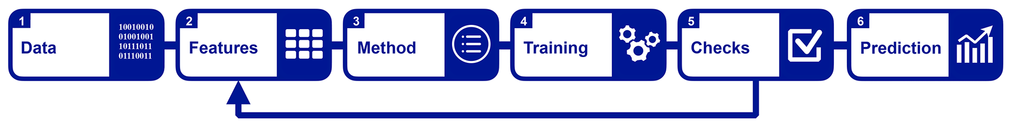
Figure 1Schematic of our machine learning workflow: the raw input data are converted into molecular representations (referred to as features in this figure). We then set up and train a machine learning method. After evaluating its performance in step 5, we may adjust the features. Once the machine learning model is calibrated and trained, we make predictions on new data.
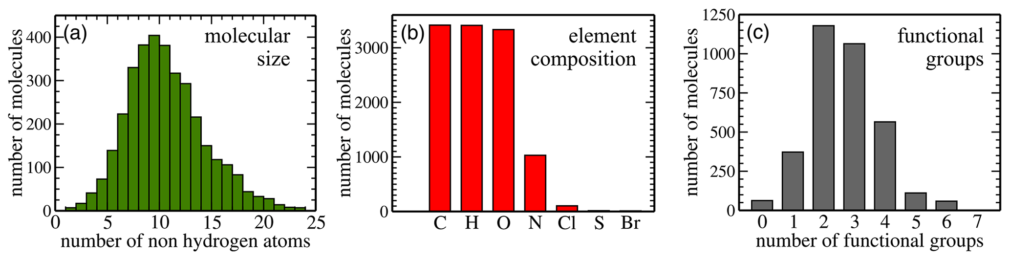
Figure 2Dataset statistics: panel (a) shows the size distribution (in terms of the number of non-hydrogen atoms) of all 3414 molecules in the dataset. Panel (b) illustrates how many molecules contain each of the chemical species, and panel (c) depicts the functional group distribution.
Our machine learning approach has six components as illustrated in Fig. 1. We start off with the raw data, which we present and analyse in Sect. 2.1. The raw data are then transformed into a suitable representation2 for machine learning (step 2). We introduce five different representations in Sect. 2.2, which we test in our machine learning model (see Sect. 3). Next we choose our machine learning method. Here we use kernel ridge regression (KRR), which is introduced in Sect. 2.3. After the machine learning model is trained in step 4, we analyse its learning success in step 5. The results of this process are shown in Sect. 3. In this step we also make adjustments to the representation and the parameters of the model to improve the learning (see the arrow from “Checks” to “Features” in Fig. 1). Finally, we use the best machine learning model to make predictions as shown in Sect. 4.
2.1 Dataset
In this work we are interested in the equilibrium partitioning coefficients of a molecule between a water-insoluble organic matter (WIOM) phase and its gas phase (KWIOM/G) as well as between the gas phase and an infinitely diluted water solution. These coefficients are defined as
where CWIOM, CW, and CG are the equilibrium concentrations of the molecule in the WIOM, water, and gas phase, respectively, at the limit of infinite dilution. In the framework of COSMOtherm calculations, gas–liquid partitioning coefficients can be converted into saturation vapour pressures, or vice versa, using the activity coefficients γW or γWIOM in the corresponding liquid (which can also be computed by COSMOtherm). Specifically, if, for example, KW/G is expressed in units of m3g−1, then , where R is the gas constant, T the temperature, M the molar mass of the compound, and KW and γW the partitioning and activity coefficients in water (Arp and Goss, 2009). This illustrates that unlike the saturation vapour pressure Psat, which is a pure compound property, the partitioning coefficient also depends on the activity of the molecule in the chosen liquid solvent, in this case water. We caution, however, that many different conventions exist e.g. for the dimensions of the partitioning coefficients and the reference states for activity coefficients – the relation given above applies only to the particular conventions used by COSMOtherm. We refer to Hyttinen et al. (2020) for a discussion on the connection between different conventions and the notation used by COSMOtherm, as well as those commonly employed in atmospheric physical chemistry.
Wang et al. (2017) used the conductor-like screening model for real solvents (COSMO-RS) theory (Klamt and Eckert, 2000; Klamt, 2011) implemented in COSMOtherm to calculate the two partitioning coefficients KWIOM/G3 and KW/G for 3414 molecules. These molecules were generated from 143 parent volatile organic compounds with the Master Chemical Mechanism (MCM) (Jenkin et al., 1997; Saunders et al., 2003) through photolysis and reactions with ozone, hydroxide radicals, and nitrate radicals.
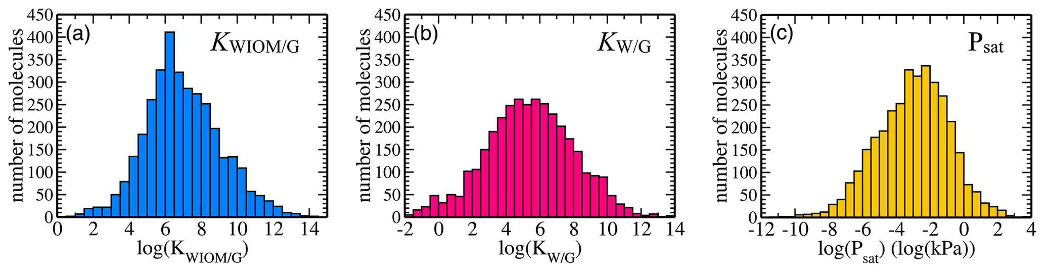
Figure 3Dataset statistics: distributions of equilibrium partitioning coefficients (a) KWIOM/G, (b) KW/G, and (c) the saturation vapour pressure Psat for all 3414 molecules in the dataset.
Here, we analyse the composition of the publicly available dataset by Wang et al. in preparation for machine learning. Figure 2 illustrates key dataset statistics. Panel (a) shows the size distribution of molecules as measured in the number of non-hydrogen atoms. The 3414 non-radical species obtained from the MCM range in size from 4 to 48 atoms, which translates into 2 to 24 non-hydrogen atoms per molecule. The distribution peaks at 10 non-hydrogen atoms and is skewed towards larger molecules. Panel (b) illustrates how many molecules contain at least one atom of the indicated element. All molecules contain carbon (100 % C); 3410 contain hydrogen (H; 99.88 %) and 3333 also oxygen (O; 97.63 %). Nitrogen (N) is the next most abundant element (30.17 %) followed by chlorine (Cl; 3.05 %), sulfur (S; 0.44 %), and bromine (Br; 0.32 %). Lastly, panel (c) presents the distribution of functional groups. It peaks at two (34 %) to three (31 %) functional groups per molecule, with relatively few molecules having zero (2 %), five (3 %), or six (2 %) functional groups. The percentages for one and four functional groups are 11 % and 17 %, respectively.
Figure 3 shows the distribution of the target properties KWIOM/G, KW/G, and Psat in Wang's dataset on a logarithmic scale. The equilibrium partitioning coefficient KWIOM/G distribution is skewed slightly towards larger coefficients, in contrast to the saturation vapour pressure Psat distribution that exhibits an asymmetry towards molecules with lower pressures. All three target properties cover approximately 15 logarithmic units and are approximately Gaussian distributed. Such peaked distributions are often not ideal for machine learning since they overrepresent molecules near the peak of the distribution and underrepresent molecules at their edges. The data peak does supply enough similarity to ensure good-quality learning, but properties of the underrepresented molecular types might be harder to learn.
We found 11 duplicate entries in Wang's dataset. These are documented in Sect. A in Table A1. The entries have the same SMILES strings and chemical formula but differ in their Master Chemical Mechanism ID. Also, the three target properties differ slightly. These duplicates did not affect the learning quality, so we did not remove them from the dataset.
Wang's dataset of 3414 molecules is relatively small for machine learning, which often requires hundreds of thousands to millions of training samples (Pyzer-Knapp et al., 2015; Smith et al., 2017; Stuke et al., 2019; Ghosh et al., 2019). A slightly larger set of Henry's law constants, which are related to KW/G, was reported by Sander (2015) for 4632 organic species. Sander's database is a collection of 17 350 Henry's law constant values collected from 689 references and therefore not as internally consistent as Wang's dataset. For example, the Sander dataset contains several molecules with multiple entries for the same property, sometimes spanning many orders of magnitude. We are not aware of a larger dataset that reports partitioning coefficients. For this reason, we rely exclusively on Wang's dataset and show that we can develop machine learning methods that are just as accurate as the underlying calculations and thus suitable for predictions.
2.2 Representations
The molecular representation for machine learning should fulfil certain requirements. It should be invariant with respect to translation and rotation of the molecule and permutations of atomic indices. Furthermore, it should be continuous, unique, compact, and efficient to compute (Faber et al., 2015; Huo and Rupp, 2017; Langer et al., 2020; Himanen et al., 2020).
In this work we employ two classes of representations for the molecular structure, also known as descriptors: physical and cheminformatics descriptors. Physical descriptors encode physical distances and angles between atoms in the material or molecule. Meanwhile, decades of research in cheminformatics have produced topological descriptors that encode the qualitative aspects of molecules in a compact representation. These descriptors are typically bit vectors, in which molecular features are encoded (hashed) into binary fingerprints, which are joined into long binary vectors. In this work, we use two physical descriptors, the Coulomb matrix and the many-body tensor, and three cheminformatics descriptors: the MACCS structural key, the topological fingerprint, and the Morgan fingerprint.
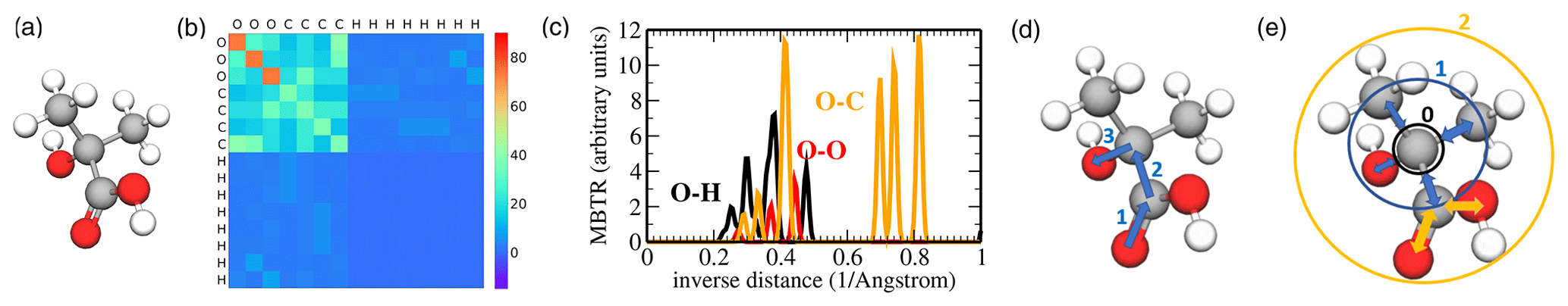
Figure 4Pictorial overview of descriptors used in this work: (a) ball-and-stick model of 2-hydroxy-2-methylpropanoic acid, (b) corresponding Coulomb matrix (CM), (c) the O–H, O–O, and O–C inverse distance entries of the many-body tensor representation (MBTR), (d) topological fingerprint (TopFP) depiction of a path with length 3, and (e) Morgan circular fingerprint with radius 0 (black), radius 1 (blue), and radius 2 (orange).
In Wang's dataset the molecular structure is encoded in SMILES (simplified molecular-input line-entry system) strings. We convert these SMILES strings into structural descriptors using Open Babel (O'Boyle et al., 2011) and the DScribe library (Himanen et al., 2020) or into cheminformatics descriptors using RDKit (Landrum, 2006).
2.2.1 Coulomb matrix
The Coulomb matrix (CM) descriptor is inspired by an electrostatic representation of a molecule (Rupp et al., 2012). It encodes the Cartesian coordinates of a molecule in a simple matrix of the form
where Ri is the coordinate of atom i with atomic charge Zi. The diagonal provides element-specific information. The coefficient and the exponent have been fitted to the total energies of isolated atoms (Rupp et al., 2012). Off-diagonal elements encode inverse distances between the atoms of the molecule by means of a Coulomb-repulsion-like term.
The dimension of the Coulomb matrix is chosen to fit the largest molecule in the dataset; i.e. it corresponds to the number of atoms of the largest molecule. The “empty” rows of Coulomb matrices for smaller molecules are padded with zeroes. Invariance with respect to the permutation of atoms in the molecule is enforced by simultaneously sorting rows and columns of each Coulomb matrix in descending order according to their ℓ2 norms. An example of a Coulomb matrix for 2-hydroxy-2-methylpropanoic acid is shown in Fig. 4b.
The CM is easily understandable, simple, and relatively small as a descriptor. However, it performs best with Laplacian kernels in the machine learning model (see Sect. 2.3), while other descriptors work better with the more standard choice of a Gaussian kernel.
2.2.2 Many-body tensor representation
The many-body tensor representation (MBTR) follows the Coulomb matrix philosophy of encoding the internal coordinates of a molecule. We will describe the MBTR only qualitatively here. Detailed equations can be found in the original publication (Huo and Rupp, 2017), our previous work (Himanen et al., 2020; Stuke et al., 2020), and Appendix B.
Unlike the Coulomb matrix, the many-body tensor is continuous and it distinguishes between different types of internal coordinates. At many-body level 1, the MBTR records the presence of all atomic species in a molecule by placing a Gaussian at the atomic number on an axis from 1 to the number of elements in the periodic table. The weight of the Gaussian is equal to the number of times the species is present in the molecule. At many-body level 2, inverse distances between every pair of atoms (bonded and non-bonded) are recorded in the same fashion. Many-body level 3 adds angular information between any triple of atoms. Higher levels (e.g. dihedral angles) would in principle be straightforward to add but are not implemented in the current MBTR versions (Huo and Rupp, 2017; Himanen et al., 2020). Figure 4c shows selected MBTR elements for 2-hydroxy-2-methylpropanoic acid.
The MBTR is a continuous descriptor, which is advantageous for machine learning. However, MBTR is by far the largest descriptor of the five we tested, and this can pose restrictions on memory and computational cost. Furthermore, the MBTR is more difficult to interpret than the CM.
2.2.3 MACCS structural key
The Molecular ACCess System (MACCS) structural key is a dictionary-based descriptor (Durant et al., 2002). It is represented as a bit vector of Boolean values that encode answers to a set of predefined questions. The MACCS structural key we used is a 166 bit long set of answers to 166 questions such as “is there an S–S bond?” or “does it contain iodine?” (Landrum, 2006; James et al., 1995).
MACCS is the smallest of the five descriptors and extremely fast to use. Its accuracy critically depends on how well the 166 questions encapsulate the chemical detail of the molecules. Is it likely to reach moderate accuracy with low computational cost and memory usage, and it could be beneficial for fast testing of a machine learning model.
2.2.4 Topological fingerprint
The topological fingerprint (TopFP) is RDKit's original fingerprint (Landrum, 2006) inspired by the Daylight fingerprint (James et al., 1995). TopFP first extracts all topological paths of certain lengths. The paths start from one atom in a molecule and travel along bonds until k bond lengths have been traversed as illustrated in Fig. 4d. The path depicted in the figure would be OCCO. The list of patterns produced is exhaustive: every pattern in the molecule, up to the path length limit, is generated. Each pattern then serves as a seed to a pseudo-random number generator (it is “hashed”), the output of which is a set of bits (typically 4 or 5 bits per pattern). The set of bits is added (with a logical OR) to the fingerprint. The length of the bit vector, maximum and minimum possible path lengths kmax and kmin, and the length of one hash can be optimized.
Topology is an informative molecular feature. We therefore expect TopFP to balance good accuracy with reasonable computational cost. However, this binary fingerprint is difficult to visualize and analyse for chemical insight.
2.2.5 Morgan fingerprint
The Morgan fingerprint is also a bit vector constructed by hashing the molecular structure. In contrast to the topological fingerprint, the Morgan fingerprint is hashed along circular or spherical paths around the central atom as illustrated in Fig. 4e. Each substructure for a hash is constructed by first numbering the atoms in a molecule with unique integers by applying the Morgan algorithm. Each uniquely numbered atom then becomes a cluster centre, around which we iteratively increase a spherical radius to include the neighbouring bonded atoms (Rogers and Hahn, 2010). Each radius increment extends the neighbour list by another molecular bond. The “circular” substructures found by the algorithm described above, excluding duplicates, are then hashed into a fingerprint (James et al., 1995; Landrum, 2006). The length of the fingerprint and the maximum radius can be optimized.
The Morgan fingerprint is quite similar to the TopFP in size and type of information encoded, so we expect similar performance. It also does not lend itself to easy chemical interpretation.
2.3 Machine learning method
2.3.1 Kernel ridge regression
In this work, we apply the kernel ridge regression (KRR) machine learning method. KRR is an example of supervised learning, in which the machine learning model is trained on pairs of input (x) and target (f) data. The trained model then predicts target values for previously unseen inputs. In this work, the input x represents the molecular descriptors CM and MBTR as well as the MACCS, TopFP, and Morgan fingerprints. The targets are scalar values for the equilibrium partitioning coefficients and saturation vapour pressures.
KRR is based on ridge regression, in which a penalty for overfitting is added to an ordinary least squares fit (Friedman et al., 2001). In KRR, unlike ridge regression, a nonlinear kernel is applied. This maps the molecular structure to our target properties in a high-dimensional space (Stuke et al., 2019; Rupp, 2015).
The target values f are a linear expansion in kernel elements:
where the sum runs over all training molecules. In this work, we use two different kernels, the Gaussian kernel,
and the Laplacian kernel,
The kernel width γ is a hyperparameter of the KRR model.
The regression coefficients αi can be solved by minimizing the error:
where yi represents reference target values for molecules in the training data. The second term is the regularization term, whose size is controlled by the hyperparameter λ. K is the kernel matrix of training inputs k(xi,xj).
This minimization problem can be solved analytically for the expansion coefficients αi.
The hyperparameters γ and λ need to be optimized separately.
We implemented KRR in Python using scikit-learn (Pedregosa et al., 2011). Our implementation has been described in Stuke et al. (2019, 2020).
2.3.2 Computational execution
Data used for supervised machine learning are typically divided into two sets: a large training set and a small test set. Both sets consists of input vectors and corresponding target properties. The KRR model is trained on the training set, and its performance is quantified on the test set. At the outset, we separate a test set of 414 molecules. From the remaining molecules, we choose six different training sets of size 500, 1000, 1500, 2000, 2500, and 3000 so that a smaller training size is always a subset of the larger one. Training the model on a sequence of such training sets allows us to compute a learning curve, which facilitates the assessment of learning success with increasing training data size. We quantify the accuracy of our KRR model by computing the mean absolute error (MAE) for the test set. To get statistically meaningful results, we repeat the training procedure 10 times. In each run, we shuffle the dataset before selecting the training and test sets so that the KRR model is trained and tested on different data each time. Each point on the learning curves is computed as the average over 10 results, and the spread serves as the standard deviation of the data point.
Model training proceeds by computing the KRR regression coefficients αi, obtained by minimizing Eq. (7). KRR hyperparameters γ and λ are typically optimized via grid search, and average optimal solutions are obtained by cross-validating the procedure. In cross-validation we split off a validation set from the training data before training the KRR model. KRR is then trained for all possible combinations of discretized hyperparameters (grid search) and evaluated on the validation set. This is done several times so that the molecules in the validation set are changed each time. Then the hyperparameter combination with minimum average cross-validation error is chosen. Our implementation of a cross-validated grid search is also based on scikit-learn (Pedregosa et al., 2011). The optimized values for γ and λ are listed in Table B2.
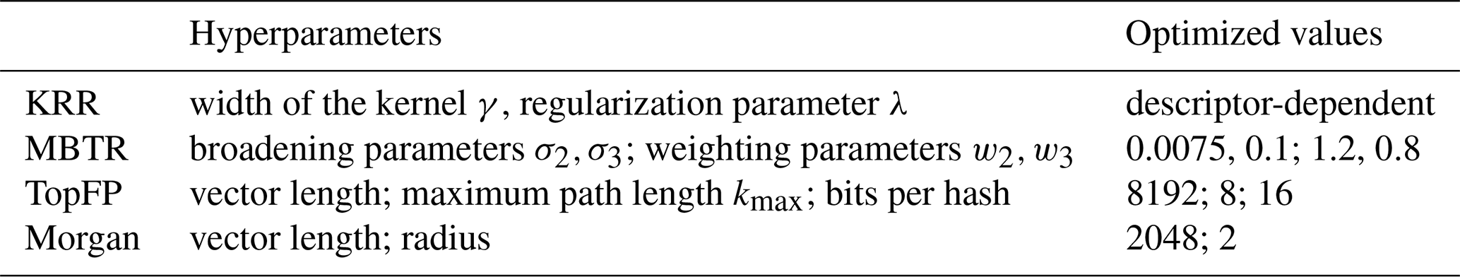
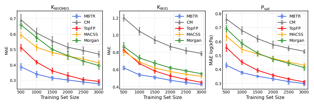
Figure 5The learning curves for equilibrium partitioning coefficients KWIOM/G, KW/G, and saturation vapour pressure Psat for predictions made with all five descriptors.
Table 1 summarizes all the hyperparameters optimized in this study, those for KRR and the molecular descriptors, and their optimal values. In the grid search, we varied both γ and λ by 10 values between 10−1 and 1010. In addition, we used two different kernels, Laplacian and Gaussian. We compared the performance of the two kernels for the average of five runs for each training size, and the most optimal kernel was chosen. In cases in which both kernels performed equally well, e.g. for the fingerprints, we chose the Gaussian kernel for its lower computational cost.
To compute the MBTR and CM descriptors we employed the Open Babel software to convert the SMILES strings provided in the Wang et al. dataset into three-dimensional molecular structures. We did not perform any conformer search. MBTR hyperparameters and TopFP hyperparameters were optimized by grid search for several training set sizes (MBTR for sizes 500, 1500, and 3000 and TopFP for sizes 1000 and 1500), and the average of two runs for each training size was taken. We did not extend the descriptor hyperparameter search to larger training set sizes, since we found that the hyperparameters were insensitive to the training set size. The MBTR weighting parameters were optimized in eighty steps between 0 (no weighting) and 1.4 and the broadening parameters in six steps between 10−1 and 10−6. The length of TopFP was varied between 1024 and 8192 (size can be varied by 2n). The range for the maximum path length extended from 5 to 11, and the bits per hash were varied between 3 and 16.
Table 2The mean average errors (MAEs) and the standard deviations for all the descriptors and target properties (equilibrium partitioning coefficients KWIOM/G, KW/G, and saturation vapour pressure Psat) with the largest possible training size of 3000.


Figure 6Scatter plots for predictions of the partitioning coefficients of a molecule between water-insoluble organic matter and the gas phase KWIOM/G, water and the gas phase KW/G, and the saturation vapour pressure Psat for the test set of 414 molecules using MBTR (top) and TopFP (bottom). The prediction with the lowest mean average error was chosen for each scatter plot.
In Fig. 5 we present the learning curves for our objectives KWIOM/G, KW/G, and Psat. Shown is the mean average error (MAE) as a function of the training set size for all three target properties and for all five molecular descriptors. As expected, the MAE decreases as the training size increases. For all target properties, the lowest errors are achieved with MBTR, and the worst-performing descriptor is CM. TopFP approaches the accuracy of MBTR as the training size increases and appears likely to outperform MBTR beyond the largest training size of 3000 molecules.
Table 2 summarizes the average MAEs and their standard deviations for the best-trained KRR model (training size of 3000 with MBTR descriptor). The highest accuracy is obtained for partitioning coefficient KWIOM/G, with a mean average error of 0.278, i.e. only 1.9 % of the entire KWIOM/G range. The second-best accuracy is obtained for saturation vapour pressure Psat with an MAE of 0.298 (or 2.0 % of the range of pressure values). The lowest accuracy is obtained for KW/G with an MAE of 0.428. However, the range for partitioning coefficient KW/G is also the largest, as seen in Fig. 3, so this amounts to only 2.7 % of the entire range of values. Our best machine learning MAEs are of the order of the COSMOtherm prediction accuracy, which lies at around a few tenths of log values (Stenzel et al., 2014; Schröder et al., 2016; van der Spoel et al., 2019).
Figure 6 shows the results for the best-performing descriptors MBTR and TopFP in more detail. The scatter plots illustrate how well the KRR predictions match the reference values. The match is further quantified by R2 values. For all three target values, the predictions hug the diagonal quite closely, and we observe only a few outliers that are further away from the diagonal. The predictions of the partitioning coefficient KWIOM/G are most accurate. This is expected because the MAE in Table 2 is lowest for this property. The largest scatter is observed for partitioning coefficient KW/G, which has the highest MAE in Table 2.
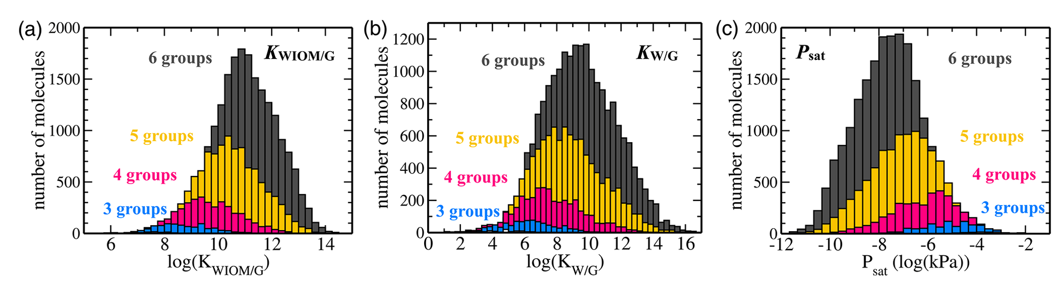
Figure 7Histograms of C10 TopFP–KRR predictions for (a) KWIOM/G, (b) KW/G, and (c) Psat. The histograms are divided into different numbers of functional groups. Molecules with two or fewer functional groups have been omitted from these histograms because their total number is very low in the C10 dataset.
Figure 8Box plot comparing C10 (in blue) with Wang's dataset (in red) for KWIOM/G, KW/G, and Psat for different numbers of functional groups. Shown are the minimum, maximum, median, and first and third quartile.
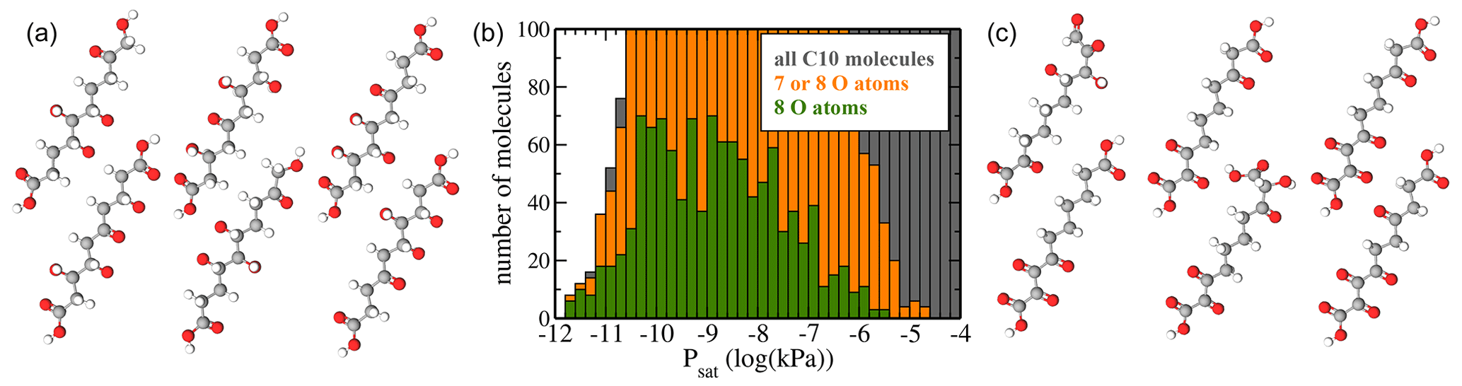
Figure 9(a) Atomic structure of the six molecules with the lowest predicted saturation vapour pressure Psat. (b) Psat histograms for molecules containing 7 or 8 O atoms (orange) or only 8 O atoms (green). For reference, the histogram of all molecules (grey) is also shown. (c) Atomic structure of the six molecules with 7 and 8 O atoms and the highest saturation vapour pressure Psat.
In the previous section we showed that our KRR model trained on the Wang et al. dataset produces low prediction errors for molecular partitioning coefficients and saturation vapour pressures and can now be employed as a fast predictor. When shown further molecular structures, it can make instant predictions for the molecular properties of interest. We demonstrate this application potential on an example dataset generated to imitate organic molecules typically found in the atmosphere.
Atmospheric oxidation reaction mechanisms can be generally classified into two main types: fragmentation and functionalization (Kroll et al., 2009; Seinfeld and Pandis, 2016). For SOA formation, functionalization is more relevant, as it leads to products with intact carbon backbones and added polar (and volatility-lowering) functional groups. Many of the most interesting molecules from an SOA-forming point of view, e.g. monoterpenes, have around 10 carbon atoms (Zhang et al., 2018). These compounds simultaneously have high enough emissions or concentrations to produce appreciable amounts of condensable products, while being large enough for those products to have low volatility.
We thus generated a dataset of molecules with a backbone of 10 carbon (C10) atoms. For simplicity, we used a linear alkane chain. In analogy to Wang's dataset, we then decorated this backbone with zero to six functional groups at different locations. We limited ourselves to the typical groups formed in “functionalizing” oxidation of VOCs by both of the main daytime oxidants OH and O3: carboxyl (-COOH), carbonyl (=O), and hydroxyl (-OH) (Seinfeld and Pandis, 2016). The (-COOH) group can only be added to the ends of the C10 molecule, while (=O) and (-OH) can be added to any carbon atom in the chain. We then generated all possible arrangements combinatorially and filtered out duplicates resulting from symmetric combinations of functional groups. In total we obtained 35 383 unique molecules. Example molecules are depicted in Fig. 9. While the functional group composition of our C10 dataset is atmospherically relevant, the particular molecules are not. The purpose of this dataset is to perform a relatively simple sanity check of the machine learning predictions on a set of compounds structurally different from those in the training dataset. We note that using e.g. more atmospherically relevant compounds such as α-pinene oxidation products for this purpose might be counterproductive, since Wang et al.'s dataset used for training contains several such compounds.
For each of the 35 383 molecules, we generated a SMILES string that serves as input for the TopFP fingerprint. We did not relax the geometry of the molecules with force fields or density functional theory. We chose TopFP as a descriptor because its accuracy is close to that of the best-performing MBTR KRR model, but it is significantly cheaper to evaluate. TopFP is also invariant to conformer choices, since the fingerprint is the same for all conformers of a molecule. We then predicted Psat, KWIOM/G, and KW/G with the TopFP–KRR model.
Figures 7 and 8 show the predictions of our TopFP–KRR model for the C10 dataset. For comparison with Wang's dataset, we broke the histograms and analysis down by the number of functional groups. For a given number of functional groups, the partitioning coefficients for our C10 dataset are somewhat higher, and the saturation vapour pressures correspondingly somewhat lower, than in Wang's dataset. This follows from the fact that our C10 molecules are on average larger4 than those contained in Wang's dataset (Fig. 2). However, as seen from Fig. 8, the averages of all three quantities (for a given number of functional groups) are not substantially different, illustrating the similarity of the two datasets. A certain degree of similarity is required to ensure predictive power, since machine learning models do not extrapolate well to data that lie outside the training range.
The variation in the studied parameters is larger in Wang's dataset for molecules with four or fewer functional groups but similar or smaller for molecules with five or six functional groups. This is likely the case because Wang's dataset contains relatively few compounds with more than four functional groups. The variation in the studied parameters (for each number of functional groups) predicted for the C10 dataset is in line with the individual group contributions predicted based on fits to experimental data, for example by the SIMPOL model (Pankow and Asher, 2008) for saturation vapour pressures. According to SIMPOL, a carboxylic acid group decreases the saturation vapour pressure at room temperature by almost a factor of 4000, while a ketone group reduces it by less than a factor of 9. Accordingly, if interactions between functional groups are ignored, a dicarboxylic acid, for example, should have a saturation vapour pressure more than 100 000 times lower than a diketone with the same carbon backbone. This is remarkably consistent with Fig. 8, where the variation of saturation vapour pressures for compounds with two functional groups in our C10 dataset is slightly more than 5 orders of magnitude.
Figure 7 illustrates the fact that the saturation vapour pressure Psat decreases with increasing number of functional groups as expected, whereas KWIOM/G and KW/G increase. This is consistent with Wang's dataset as shown in Fig. 8, where we compare averages between the two datasets. The magnitude of the decrease (increase) amounts to approximately 1 or 2 orders of magnitude per functional group and is, again, consistent with existing structure–activity relationships based on experimental data (e.g. Pankow and Asher, 2008; Compernolle et al., 2011; Nannoolal et al., 2008).
The region of low Psat is most relevant for atmospheric SOA formation. However, we caution that COSMOtherm predictions have not yet been properly validated against experiments for this pressure regime. As discussed above, we can hope for order-of-magnitude accuracy at best. Figure 9b shows histograms of only molecules with 7 or 8 oxygen atoms. These are compared to the full dataset. Since the “8 O atom set” is a subset of the “7 or 8 O atoms” set, which in turn is a subset of “all molecules”, the lengths of the bars in a given bin reflect the percentages of molecules with 7 or 8 O atoms. We observe that below 10−10 kPa, almost all C10 molecules contain 7 or 8 O atoms, as there is little grey visible in that part of the histogram. In the context of atmospheric chemistry, the least-volatile fraction of our C10 dataset corresponds to LVOCs (low-volatility organic compounds), which are capable of condensing onto small aerosol particles but not actually forming them. Our results are thus in qualitative agreement with recent experimental results by Peräkylä et al. (2020), who concluded that the highly oxidized C10 products of α-pinene oxidation are mostly LVOCs. However, we note that the compounds measured by Peräkylä et al. are likely to contain functional groups not included in our C10 dataset, as well as structural features such as branching and rings.
Figure 9a and c show the molecular structures of the lowest-volatility compounds and the highest-volatility compounds with 7 or 8 O atoms, respectively. The six shown highest-volatility compounds inevitably contain at least one carboxylic acid group, as we have restricted the number of functional groups to six or fewer, and only the acid groups contain two oxygen atoms. Comparing the two sets, we see that the lowest-volatility compounds contain more hydroxyl groups and fewer ketone groups, while the highest-volatility compounds with 7 or 8 oxygen atoms contain almost no hydroxyl groups. This is expected, since e.g. a hydroxyl group lowers the saturation vapour pressure by over a factor of 100 at 298 K, while the effect of a ketone group is, as previously noted, less than a factor of 9 according to the SIMPOL model (Pankow and Asher, 2008). However, even the lowest-volatility compounds (Fig. 9a) contain a few ketone groups such that the numbers of hydrogen-bond donor and acceptor groups are roughly similar. This result demonstrates that unlike the simplest group contribution models such as SIMPOL, which would invariably predict that the lowest-volatility compounds in our C10 dataset should be the tetrahydroxydicarboxylic acids, both the original COSMOtherm predictions and the machine learning model based on them are capable of accounting for hydrogen-bonding interactions between functional groups. As we did not include conformational information for our C10 molecules in the machine learning predictions, this is most likely due to structural similarities between the C10 compounds and hydrogen-bonding molecules in the training dataset.
Lastly, we consider the issue of non-unique descriptors. Although the cheminformatics descriptors are fast to compute and use, a duplicate check revealed that it is possible to obtain identical descriptors for different molecule structures, even for this relatively small pool of molecules. The MACCS fingerprint in particular produced over 500 duplicates (about 15 % of the dataset) because its query list is not sufficiently descriptive of this molecule class. Some duplicates were also observed for TopFP (<1.5 %), whereas physical descriptors were both entirely unique, as expected. The original dataset itself contained 11 identical molecular structures labelled with different SMILES strings, as mentioned in Sect. 2.1. Machine learning model checks revealed that the number of duplicates in this study was small enough to have a negligible effect on predictions (apart from the MACCS key models), so we did not purge them.
In this study, we set out to evaluate the potential of the KRR machine learning method to map molecular structures to its atmospheric partitioning behaviour and establish which molecular descriptor has the best predictive capability.
KRR is a relatively simple kernel-based machine learning technique that is straightforward to implement and fast to train. Given model simplicity, the quality of learning depends strongly on the information content of the molecular descriptor. More specifically, it hinges on how well each format encapsulates the structural features relevant to the atmospheric behaviour. The exhaustive approach of the MBTR descriptor to documenting molecular features has led to very good predictive accuracy in machine learning of molecular properties (Stuke et al., 2019; Langer et al., 2020; Rossi and Cumby, 2020; Himanen et al., 2020), and this work is no exception. The lightweight CM descriptor does not perform nearly as well, but these two representations from physical sciences provide us with an upper and lower limit on predictive accuracy.
Descriptors from cheminformatics that were developed specifically for molecules have variable performance. Between them, the topological fingerprint leads to the best learning quality that approaches MBTR accuracy in the limit of larger training set sizes. This is a notable finding, not least because the relatively small TopFP data structures in comparison to MBTR reduce the computational time and memory required for machine learning. MBTR encoding requires knowledge of the three-dimensional molecular structure, which raises the issue of conformer search. It is unclear which molecular conformers are relevant for atmospheric condensation behaviour, and COSMOtherm calculations on different conformers can produce values that are orders of magnitude apart. TopFP requires only connectivity information and can be built from SMILES strings, eliminating any conformer considerations (albeit at the cost of possibly losing some information on e.g. intramolecular hydrogen bonds). All this makes TopFP the most promising descriptor for future machine learning studies in atmospheric science that we have identified in this work.
Our results show that KRR can be used to train a model to predict COSMOtherm saturation vapour pressures, with error margins smaller than those of the original COSMOtherm predictions. In the future, we will extend our training set to especially encompass atmospheric autoxidation products (Bianchi et al., 2019), which are not included in existing saturation vapour pressure datasets and for which existing prediction methods are highly uncertain. We also intend to extend the machine learning model to predict a larger set of parameters computed by COSMOtherm, such as vaporization enthalpies, internal energies of phase transfer, and activity coefficients in representative phases. While COSMOtherm predictions for complex molecules such as autoxidation products also have large uncertainties, a fast and efficient “COSMOtherm-level” KRR predictor would still be immensely useful, for example, for assessing whether a given compound is likely to have extremely low volatility or not. Experimental volatility data for such compounds are also gradually becoming available, either through indirect inference methods such as Peräkylä et al. (2020) or, for example, from thermal desorption measurements (Li et al., 2020). These can then be used to constrain and anchor the model and also ultimately yield quantitatively reliable volatility predictions.
Table A1 Duplicates found in Wang et al.'s dataset: listed are the index in the dataset, the ID in the Master Chemical Mechanism (MCM_ID), the corresponding SMILES string, the chemical formula, and the three target properties (KWIOM/G, KW/G, and Psat).
In this Appendix we provide the mathematical structure of the MBTR as it is implemented in the DScribe library (Himanen et al., 2020). The many-body levels in the MBTR are denoted as k. For , and 3, geometry functions encode the different features: g1(Zl)=Zl (atomic number), (distance), or (inverse distance), and (cosine of angle).
The scalar values returned by the geometry functions gk are Gaussian-broadened into continuous representations 𝒟k.
The σk values are the feature widths for the different k levels, and x runs over a predefined range of possible values for the geometry functions gk.
Finally, a weighted sum of distributions 𝒟k is generated for each possible combination of chemical elements present in the dataset.
The sums for l, m, and n run over all atoms with atomic numbers Z1, Z2, and Z3. wk represents weighting functions that balance the relative importance of different k terms and/or limit the range of inter-atomic interactions. For k=1, usually no weighting is used (). For k=2 and k=3 the following exponential decay functions are implemented in DScribe.
The parameter sk effectively tunes the cutoff distance. The functions MBTRk(x) are then discretized with nk many points in the respective intervals .
Table B1 Values of the optimal KRR hyperparameter λ obtained by cross-validation as a function of descriptor type and training set size. The procedure was repeated 10 times with re-shuffled data. Average values () were used in further KRR models. We also report the statistical standard deviation Δλ.

Table B2 Values of the optimal KRR hyperparameter γ obtained by cross-validation as a function of descriptor type and training set size. The procedure was repeated 10 times with re-shuffled data. Average values () were used in further KRR models. We also report the statistical standard deviation Δγ.
The Wang dataset (Wang et al., 2017) and the novel C10 dataset of atmospheric molecules (https://doi.org/10.5281/zenodo.4291795, Lumiaro, 2020) are freely available online. The KRR code employed in this study can be found on GitLab (https://gitlab.com/cest-group/krr-and-atmospheric-molecules, Gitlab, 2020).
EL performed all computational work. MT advised on the computations. PR, HV, and TK conceived the study. All authors participated in drafting the paper.
The authors declare that they have no conflict of interest.
Publisher's note: Copernicus Publications remains neutral with regard to jurisdictional claims in published maps and institutional affiliations.
This work was supported by COST (European Cooperation in Science and Technology) Action 18234, the University of Helsinki Faculty of Science ATMATH project, and the Academy of Finland through their flagship programme: Finnish Center for Artificial Intelligence, FCAI. We thank CSC, the Finnish IT Center for Science, and Aalto Science IT for computational resources.
This research has been supported by the Academy of Finland (grant nos. 315600 and 316601) and the European Research Council, H2020 (grant no. DAMOCLES (692891)).
This paper was edited by Gordon McFiggans and reviewed by Frank Wania and two anonymous referees.
Arp, H. P. H. and Goss, K.-U.: Ambient Gas/Particle Partitioning. 3. Estimating Partition Coefficients of Apolar, Polar, and Ionizable Organic Compounds by Their Molecular Structure, Environ. Sci. Technol., 43, 1923–1929, 2009. a
Barnes, E. A., Hurrell, J. W., Ebert-Uphoff, I., Anderson, C., and Anderson, D.: Viewing Forced Climate Patterns Through an AI Lens, Geophys. Res. Lett., 46, 13389–13398, 2019. a, b
Bartók, A. P., De, S., Poelking, C., Bernstein, N., Kermode, J. R., Csányi, G., and Ceriotti, M.: Machine learning unifies the modeling of materials and molecules, Sci. Adv., 3, e1701816, https://doi.org/10.1126/sciadv.1701816, 2017. a
Bianchi, F., Kurtén, T., Riva, M., Mohr, C., Rissanen, M. P., Roldin, P., Berndt, T., Crounse, J. D., Wennberg, P. O., Mentel, T. F., Wildt, J., Junninen, H., Jokinen, T., Kulmala, M., Worsnop, D. R., Thornton, J. A., Donahue, N., Kjaergaard, H. G., and Ehn, M.: Highly Oxygenated Organic Molecules (HOM) from Gas-Phase Autoxidation Involving Peroxy Radicals: A Key Contributor to Atmospheric Aerosol, Chem. Rev., 119, 3472–3509, 2019. a, b
Bilde, M., Barsanti, K., Booth, M., Cappa, C. D., Donahue, N. M., Emanuelsson, E. U., McFiggans, G., Krieger, U. K., Marcolli, C., Topping, D., Ziemann, P., Barley, M., Clegg, S., Dennis-Smither, B., Hallquist, M., Hallquist, Å. M., Khlystov, A., Kulmala, M., Mogensen, D., Percival, C. J., Pope, F., Reid, J. P., Ribeiro da Silva, M. A. V., Rosenoern, T., Salo, K., Soonsin, V. P., Yli-Juuti, T., Prisle, N. L., Pagels, J., Rarey, J., Zardini, A. A., and Riipinen, I.: Saturation Vapor Pressures and Transition Enthalpies of Low-Volatility Organic Molecules of Atmospheric Relevance: From Dicarboxylic Acids to Complex Mixtures, Chem. Rev., 115, 4115–4156, 2015. a
Cervone, G., Franzese, P., Ezber, Y., and Boybeyi, Z.: Risk assessment of atmospheric emissions using machine learning, Nat. Hazards Earth Syst. Sci., 8, 991–1000, https://doi.org/10.5194/nhess-8-991-2008, 2008. a, b
Coley, C. W., Eyke, N. S., and Jensen, K. F.: Autonomous Discovery in the Chemical Sciences Part I: Progress, Angew. Chem. Int. Ed.. 59, 22858, https://doi.org/10.1002/anie.201909987, 2020a. a
Coley, C. W., Eyke, N. S., and Jensen, K. F.: Autonomous Discovery in the Chemical Sciences Part II: Outlook, Angew. Chem. Int. Ed., 59, 23414, https://doi.org/10.1002/anie.201909989, 2020b. a
Compernolle, S., Ceulemans, K., and Müller, J.-F.: EVAPORATION: a new vapour pressure estimation methodfor organic molecules including non-additivity and intramolecular interactions, Atmos. Chem. Phys., 11, 9431–9450, https://doi.org/10.5194/acp-11-9431-2011, 2011. a, b
Durant, J. L., Leland, B. A., Henry, D. R., and Nourse, J. G.: Reoptimization of MDL Keys for Use in Drug Discovery, J. Chem. Inf. Comp. Sci., 42, 1273–1280, 2002. a, b
Eckert, F. and Klamt, A.: Fast solvent screening via quantum chemistry: COSMO-RS approach, AIChE J., 48, 369–385, 2002. a, b
Elm, J., Kubečka, J., Besel, V., Jääskeläinen, M. J., Halonen, R., Kurtén, T., and Vehkamäki, H.: Modeling the formation and growth of atmospheric molecular clusters: A review, J. Aerosol Sci., 149, 105621, https://doi.org/10.1016/j.jaerosci.2020.105621, 2020. a
Faber, F., Lindmaa, A., Lilienfeld, O. A. v., and Armiento, R.: Crystal structure representations for machine learning models of formation energies, Int. J. Quantum Chem., 115, 1094–1101, 2015. a
Fang, L., Makkonen, E., Todorović, M., Rinke, P., and Chen, X.: Efficient Amino Acid Conformer Search with Bayesian Optimization, J. Chem. Theory Comput., 17, 1955–1966, 2021. a
Friedman, J., Hastie, T., and Tibshirani, R.: The elements of statistical learning, vol. 1, Springer Series in Statistics, New York, 2001. a
Ghosh, K., Stuke, A., Todorović, M., Jørgensen, P. B., Schmidt, M. N., Vehtari, A., and Rinke, P.: Deep Learning Spectroscopy: Neural Networks for Molecular Excitation Spectra, Adv. Sci., 6, 1801367, https://doi.org/10.1002/advs.201801367, 2019. a, b
Gitlab: KRR for Atmospheric molecules, available at: https://gitlab.com/cest-group/krr-and-atmospheric-molecules (last access: August 2021), 2020. a
Goldsmith, B. R., Esterhuizen, J., Liu, J.-X., Bartel, C. J., and Sutton, C.: Machine learning for heterogeneous catalyst design and discovery, AIChE J., 64, 2311–2323, 2018. a
Gómez-Bombarelli, R., Aguilera-Iparraguirre, J., Hirzel, T. D., Duvenaud, D., Maclaurin, D., Blood-Forsythe, M. A., Chae, H. S., Einzinger, M., Ha, D.-G., Wu, T. C.-C., Markopoulos, G., Jeon, S., Kang, H., Miyazaki, H., Numata, M., Kim, S., Huang, W., Hong, S. I., Baldo, M. A., Adams, R. P., and Aspuru-Guzik, A.: Design of efficient molecular organic light-emitting diodes by a high-throughput virtual screening and experimental approach, Nat. Mater., 15, 1120–1127, 2016. a
Goss, K.-U.: The Air/Surface Adsorption Equilibrium of Organic Compounds Under Ambient Conditions, Crit. Rev. Env. Sci. Tec., 34, 339–389, 2004. a
Goss, K.-U.: Prediction of the temperature dependency of Henry's law constant using poly-parameter linear free energy relationships, Chemosphere, 64, 1369–1374, 2006. a
Goss, K.-U. and Schwarzenbach, R. P.: Linear Free Energy Relationships Used To Evaluate Equilibrium Partitioning of Organic Compounds, Environ. Sci. Technol., 35, 1–9, 2001. a
Gu, G. H., Noh, J., Kim, I., and Jung, Y.: Machine learning for renewable energy materials, J. Mater. Chem. A, 7, 17096–17117, 2019. a
Hilal, S. H., Ayyampalayam, S. N., and Carreira, L. A.: Air-Liquid Partition Coefficient for a Diverse Set of Organic Compounds: Henry's Law Constant in Water and Hexadecane, Environ. Sci. Technol., 42, 9231–9236, 2008. a
Himanen, L., Geurts, A., Foster, A. S., and Rinke, P.: Data-Driven Materials Science: Status, Challenges, and Perspectives, Adv. Sci., 6, 1900808, https://doi.org/10.1002/advs.201900808, 2019. a
Himanen, L., Jäger, M. O. J., Morooka, E. V., Canova, F. F., Ranawat, Y. S., Gao, D. Z., Rinke, P., and Foster, A. S.: DScribe: Library of descriptors for machine learning in materials science, Comput. Phys. Commun., 247, 106949, https://doi.org/10.1016/j.cpc.2019.106949, 2020. a, b, c, d, e, f, g, h
Huntingford, C., Jeffers, E. S., Bonsall, M. B., Christensen, H. M., Lees, T., and Yang, H.: Machine learning and artificial intelligence to aid climate change research and preparedness, Environ. Res. Lett., 14, 124007, https://doi.org/10.1088/1748-9326/ab4e55, 2019. a, b
Huo, H. and Rupp, M.: Unified Representation for Machine Learning of Molecules and Crystals, arXiv: preprint: arXiv:1704.06439, 2017. a, b, c, d
Hyttinen, N., Elm, J., Malila, J., Calderón, S. M., and Prisle, N. L.: Thermodynamic properties of isoprene- and monoterpene-derived organosulfates estimated with COSMOtherm, Atmos. Chem. Phys., 20, 5679–5696, https://doi.org/10.5194/acp-20-5679-2020, 2020. a, b
Hyttinen, N., Wolf, M., Rissanen, M. P., Ehn, M., Peräkylä, O., Kurtén, T., and Prisle, N. L.: Gas-to-Particle Partitioning of Cyclohexene- and α-Pinene-Derived Highly Oxygenated Dimers Evaluated Using COSMOtherm, J. Phys. Chem. A, 125, 3726–3738, 2021. a
IPCC, Climate Change 2013: The Physical Science Basis. Contribution of Working Group I to the Fifth Assessment Report of the Intergovernmental Panel on Climate Change, edited by: Stocker, T. F., Qin, D., Plattner, G.-K., Tignor, M., Allen, S. K., Boschung, J., Nauels, A., Xia, Y. Bex, V., and Midgley, P. M., Cambridge University Press, Cambridge, UK and New York, NY, USA, 1535 pp., 2013. a
James, C., Weininger, D., and Delany, J.: Daylight Theory Manual. Daylight Chemical Information Systems, Inc., Irvine, CA, 1995. a, b, c, d
Jenkin, M. E., Saunders, S. M., and Pilling, M. J.: The tropospheric degradation of volatile organic compounds: a protocol for mechanism development, Atmos. Environ., 31, 81–104, 1997. a, b
Kalberer, M., Paulsen, D., Sax, M., Steinbacher, M., Dommen, J., Prevot, A. S. H., Fisseha, R., Weingartner, E., Frankevich, V., Zenobi, R., and Baltensperger, U.: Identification of Polymers as Major Components of Atmospheric Organic Aerosols, Science, 303, 1659–1662, 2004. a
Klamt, A.: The COSMO and COSMO-RS solvation models, WIREs Comput. Mol. Sci., 1, 699–709, 2011. a, b
Klamt, A. and Eckert, F.: COSMO-RS: a novel and efficient method for the a priori prediction of thermophysical data of liquids, Fluid Phase Equilibr., 172, 43–72, 2000. a, b, c, d
Klamt, A. and Eckert, F.: Erratum to COSMO-RS: a novel and efficient method for the a priori prediction of thermophysical data of liquids, [Fluid Phase Equilibr. 172, 43–72, 2000], Fluid Phase Equilibr., 205, 357, https://doi.org/10.1016/S0378-3812(00)00357-5, 2003. a
Kroll, J. H., Smith, J. D., Che, D. L., Kessler, S. H., Worsnop, D. R., and Wilson, K. R.: Measurement of fragmentation and functionalization pathways in the heterogeneous oxidation of oxidized organic aerosol, Phys. Chem. Chem. Phys., 11, 8005–8014, 2009. a
Landrum, G.: RDKit: Open-source cheminformatics, available at: http://www.rdkit.org/ (last access: 27 August 2021), 2006. a, b, c, d, e
Langer, M. F., Goeßmann, A., and Rupp, M.: Representations of molecules and materials for interpolation of quantum-mechanical simulations via machine learning, arXiv preprint, arXiv:2003.12081, 2020. a, b, c
Li, Z., D'Ambro, E. L., Schobesberger, S., Gaston, C. J., Lopez-Hilfiker, F. D., Liu, J., Shilling, J. E., Thornton, J. A., and Cappa, C. D.: A robust clustering algorithm for analysis of composition-dependent organic aerosol thermal desorption measurements, Atmos. Chem. Phys., 20, 2489–2512, https://doi.org/10.5194/acp-20-2489-2020, 2020. 2020. a
Lumiaro, E., Todorović, M., Rinke, P., Kurten, T., and Vehkamäki, H.: Atmospheric C10 dataset, Zenodo [data set], https://doi.org/10.5281/zenodo.4291795, 2020. a
Ma, J., Sheridan, R. P., Liaw, A., Dahl, G. E., and Svetnik, V.: Deep Neural Nets as a Method for Quantitative Structure–Activity Relationships, J. Chem. Inf. Model., 55, 263–274, 2015. a
Masuda, R., Iwabuchi, H., Schmidt, K. S., Damiani, A., and Kudo, R.: Retrieval of Cloud Optical Thickness from Sky-View Camera Images using a Deep Convolutional Neural Network based on Three-Dimensional Radiative Transfer, Remote Sens.-Basel, 11, 1962, https://doi.org/10.3390/rs11171962, 2019. a, b
Meyer, B., Sawatlon, B., Heinen, S., von Lilienfeld, O. A., and Corminboeuf, C.: Machine learning meets volcano plots: computational discovery of cross-coupling catalysts, Chem. Sci., 9, 7069–7077, 2018. a
Morgan, H. L.: The Generation of a Unique Machine Description for Chemical Structures-A Technique Developed at Chemical Abstracts Service, J. Chem. Doc., 5, 107–113, 1965. a
Müller, T., Kusne, A. G., and Ramprasad, R.: Machine Learning in Materials Science, chap. 4, pp. 186–273, John Wiley and Sons, Ltd, Hoboken, New Jersey, USA, 2016. a
Nannoolal, Y., Rarey, J., and Ramjugernath, D.: Estimation of pure component properties: Part 3. Estimation of the vapor pressure of non-electrolyte organic compounds via group contributions and group interactions, Fluid Phase Equilibr., 269, 117–133, 2008. a, b
Nourani, V., Uzelaltinbulat, S., Sadikoglu, F., and Behfar, N.: Artificial Intelligence Based Ensemble Modeling for Multi-Station Prediction of Precipitation, Atmosphere, 10, 80, https://doi.org/10.3390/atmos10020080, 2019. a, b
O'Boyle, N. M., Banck, M., James, C. A., Morley, C., Vandermeersch, T., and Hutchison, G. R.: Open Babel: An open chemical toolbox, J. Cheminformatics, 3, 33, 2011. a
Pankow, J. F. and Asher, W. E.: SIMPOL.1: a simple group contribution method for predicting vapor pressures and enthalpies of vaporization of multifunctional organic compounds, Atmos. Chem. Phys., 8, 2773–2796, https://doi.org/10.5194/acp-8-2773-2008, 2008. a, b, c, d
Pedregosa, F., Varoquaux, G., Gramfort, A., Michel, V., Thirion, B., Grisel, O., Blondel, M., Prettenhofer, P., Weiss, R., Dubourg, V., Vanderplas, J., Passos, A., Cournapeau, D., Brucher, M., Perrot, M., and Duchesnay, É.: Scikit-learn: Machine learning in Python, J. Mach. Learn. Res., 12, 2825–2830, 2011. a, b
Peräkylä, O., Riva, M., Heikkinen, L., Quéléver, L., Roldin, P., and Ehn, M.: Experimental investigation into the volatilities of highly oxygenated organic molecules (HOMs), Atmos. Chem. Phys., 20, 649–669, https://doi.org/10.5194/acp-20-649-2020, 2020. a, b
Pyzer-Knapp, E. O., Li, K., and Aspuru Guzik, A.: Learning from the Harvard Clean Energy Project: The Use of Neural Networks to Accelerate Materials Discovery, Adv. Funct. Mater, 25, 6495–6502, 2015. a
Raventos-Duran, T., Camredon, M., Valorso, R., Mouchel-Vallon, C., and Aumont, B.: Structure-activity relationships to estimate the effective Henry's law constants of organics of atmospheric interest, Atmos. Chem. Phys., 10, 7643–7654, https://doi.org/10.5194/acp-10-7643-2010, 2010. a
Rogers, D. and Hahn, M.: Extended-connectivity fingerprints, J. Chem. Inf. Model., 50, 742–754, 2010. a
Rossi, K. and Cumby, J.: Representations and descriptors unifying the study of molecular and bulk systems, Int. J. Quantum Chem., 120, e26151, https://doi.org/10.1002/qua.26151, 2020. a, b
Rupp, M.: Machine learning for quantum mechanics in a nutshell, Int. J. Quantum Chem., 115, 1058–1073, 2015. a
Rupp, M., Tkatchenko, A., Müller, K.-R., and von Lilienfeld, O. A.: Fast and Accurate Modeling of Molecular Atomization Energies with Machine Learning, Phys. Rev. Lett., 108, 058301, https://doi.org/10.1103/PhysRevLett.108.058301, 2012. a, b, c
Rupp, M., von Lilienfeld, O. A., and Burke, K.: Guest Editorial: Special Topic on Data-Enabled Theoretical Chemistry, J. Chem. Phys., 148, 241401, https://doi.org/10.1063/1.5043213, 2018. a
Sander, R.: Compilation of Henry's law constants (version 4.0) for water as solvent, Atmos. Chem. Phys., 15, 4399–4981, https://doi.org/10.5194/acp-15-4399-2015, 2015. a
Saunders, S. M., Jenkin, M. E., Derwent, R. G., and Pilling, M. J.: Protocol for the development of the Master Chemical Mechanism, MCM v3 (Part A): tropospheric degradation of non-aromatic volatile organic compounds, Atmos. Chem. Phys., 3, 161–180, https://doi.org/10.5194/acp-3-161-2003, 2003. a, b
Schmidt, J., Marques, M. R. G., Botti, S., and Marques, M. A. L.: Recent advances and applications of machine learning in solid-state materials science, npj Comput. Mater., 5, 83, https://doi.org/10.1038/s41524-019-0221-0, 2019. a
Schröder, B., Fulem, M., and M. A. R. Martins: Vapor pressure predictions of multi-functional oxygen-containing organic compounds with COSMO-RS, Atmos. Environ., 133, 135–144, 2016. a
Seinfeld, J. H. and Pandis, S. N.: Atmospheric Chemistry and Physics: From Air Pollution to Climate Change, 3rd Edn., Wiley, New Jersey, 2016. a, b
Shandiz, M. A. and Gauvin, R.: Application of machine learning methods for the prediction of crystal system of cathode materials in lithium-ion batteries, Comput. Mater. Sci., 117, 270–278, 2016. a
Shrivastava, M., Cappa, C. D., Fan, J., Goldstein, A. H., Guenther, A. B., Jimenez, J. L., Kuang, C., Laskin, A., Martin, S. T., Ng, N. L., Petaja, T., Pierce, J. R., Rasch, P. J., Roldin, P., Seinfeld, J. H., Shilling, J., Smith, J. N., Thornton, J. A., Volkamer, R., Wang, J., Worsnop, D. R., Zaveri, R. A., Zelenyuk, A., and Zhang, Q.: Recent advances in understanding secondary organic aerosol: Implications for global climate forcing, Rev. Geophys., 55, 509–559, https://doi.org/10.1002/2016RG000540, 2017. a
Shrivastava, M., Andreae, M. O., Artaxo, P., Barbosa, H. M. J., Berg, L. K., Brito, J., Ching, J., Easter, R. C., Fan, J., Fast, J. D., Feng, Z., Fuentes, J. D., Glasius, M., Goldstein, A. H., Alves, E. G., Gomes, H., Gu, D., Guenther, A., Jathar, S. H., Kim, S., Liu, Y., Lou, S., Martin, S. T., McNeill, V. F., Medeiros, A., de Sá, S. S., Shilling, J. E., Springston, S. R., Souza, R. A. F., Thornton, J. A., Isaacman-VanWertz, G., Yee, L. D., Ynoue, R., Zaveri, R. A., Zelenyuk, A., and Zhao, C.: Urban pollution greatly enhances formation of natural aerosols over the Amazon rainforest, Nat. Commun., 10, 1046, https://doi.org/10.1038/s41467-019-08909-4, 2019. a
Smith, J. S., Isayev, O., and Roitberg, A. E.: ANI-1: an extensible neural network potential with DFT accuracy at force field computational cost, Chem. Sci., 8, 3192–3203, 2017. a
Stenzel, A., Goss, K.-U., and Endo, S.: Prediction of partition coefficients for complex environmental contaminants: Validation of COSMOtherm, ABSOLV, and SPARC, Environ. Toxicol. Chem., 33, 1537–1543, 2014. a
Stuke, A., Todorović, M., Rupp, M., Kunkel, C., Ghosh, K., Himanen, L., and Rinke, P.: Chemical diversity in molecular orbital energy predictions with kernel ridge regression, J. Chem. Phys., 150, 204121, https://doi.org/10.1063/1.5086105, 2019. a, b, c, d, e
Stuke, A., Rinke, P., and Todorović, M.: Efficient hyperparameter tuning for kernel ridge regression with Bayesian optimization, arXiv: preprint, arXiv:2004.00675, 2020. a, b
Todorović, M., Gutmann, M. U., Corander, J., and Rinke, P.: Bayesian inference of atomistic structure in functional materials, npj Comput. Mater., 5, 35, https://doi.org/10.1038/s41524-019-0175-2, 2019. a
Toms, B. A., Kashinath, K., Prabhat, M., Mudigonda, M., and Yang, D.: Climate Science, Deep Learning, and Pattern Discovery: The Madden-Julian Oscillation as a Test Case, in: vol. 2018, AGU Fall Meeting Abstracts, 11 December 2018, Walter E Washington Convention Center, IN21D–0738, 2018. a, b
Topping, D., Barley, M., Bane, M. K., Higham, N., Aumont, B., Dingle, N., and McFiggans, G.: UManSysProp v1.0: an online and open-source facility for molecular property prediction and atmospheric aerosol calculations, Geosci. Model Dev., 9, 899–914, https://doi.org/10.5194/gmd-9-899-2016, 2016. a
Valorso, R., Aumont, B., Camredon, M., Raventos-Duran, T., Mouchel-Vallon, C., Ng, N. L., Seinfeld, J. H., Lee-Taylor, J., and Madronich, S.: Explicit modelling of SOA formation from α-pinene photooxidation: sensitivity to vapour pressure estimation, Atmos. Chem. Phys., 11, 68956910, https://doi.org/10.5194/acp-11-6895-2011, 2011. a
van der Spoel, D., Manzetti, S., Zhang, H., and Klamt, A.: Prediction of Partition Coefficients of Environmental Toxins Using Computational Chemistry Methods, ACS Omega, 4, 13772–13781, 2019. a
Wang, C., Yuan, T., Wood, S. A., Goss, K.-U., Li, J., Ying, Q., and Wania, F.: Uncertain Henry's law constants compromise equilibrium partitioning calculations of atmospheric oxidation products, Atmos. Chem. Phys., 17, 7529–7540, https://doi.org/10.5194/acp-17-7529-2017, 2017. a, b, c
Ye, Q., Robinson, E. S., Ding, X., Ye, P., Sullivan, R. C., and Donahue, N. M.: Mixing of secondary organic aerosols versus relative humidity, P. Natl. Acad. Sci. USA, 113, 12649–12654, 2016. a
Zhang, H., Yee, L. D., Lee, B. H., Curtis, M. P., Worton, D. R., Isaacman-VanWertz, G., Offenberg, J. H., Lewandowski, M., Kleindienst, T. E., Beaver, M. R., Holder, A. L., Lonneman, W. A., Docherty, K. S., Jaoui, M., Pye, H. O. T., Hu, W., Day, D. A., Campuzano-Jost, P., Jimenez, J. L., Guo, H., Weber, R. J., de Gouw, J., Koss, A. R., Edgerton, E. S., Brune, W., Mohr, C., Lopez-Hilfiker, F. D., Lutz, A., Kreisberg, N. M., Spielman, S. R., Hering, S. V., Wilson, K. R., Thornton, J. A., and Goldstein, A. H.: Monoterpenes are the largest source of summertime organic aerosol in the southeastern United States, P. Natl. Acad. Sci. USA, 115, 2038–2043, 2018. a
Zunger, A.: Inverse design in search of materials with target functionalities, Nat. Rev. Chem., 2, 0121, https://doi.org/10.1038/s41570-018-0121, 2018. a
The gas–octanol partitioning coefficient (KO/G) can then be obtained to good approximation from these by division.
We use the words “representation” and “features” interchangeably.
As a model WIOM phase Wang et al. used a compound originally suggested by Kalberer et al. (2004) as a representative secondary organic aerosol constituent. The IUPAC name for the compound in question, with elemental composition C14H16O5, is 1-(5-(3,5-dimethylphenyl)dihydro-[1,3]dioxolo[4,5-d][1,3]dioxol-2-yl)ethan-1-one.
Our C10 molecules range in size from 10 to 18 non-hydrogen atoms since the largest of our molecules contains two carboxylic acid and four ketone and/or hydroxyl groups.