Methane (CH₄) sources in Krakow, Poland: insights from isotope analysis

Methane (CH₄) emissions from human activities are a threat to the resilience of our current climate system. The stable isotopic composition of methane (δ¹³C and δ²H) allows us to distinguish between the different CH₄ origins. A significant part of the European CH₄ emissions, 3.6 % in 2018, comes from coal extraction in Poland, the Upper Silesian Coal Basin (USCB) being the main hotspot.
Measurements of CH₄ mole fraction (χ(CH₄)), δ¹³C, and δ²H in CH₄ in ambient air were performed continuously during 6 months in 2018 and 2019 at Krakow, Poland, in the east of the USCB. In addition, air samples were collected during parallel mobile campaigns, from multiple CH₄ sources in the footprint area of the continuous measurements. The resulting isotopic signatures from sampled plumes allowed us to distinguish between natural gas leaks, coal mine fugitive emissions, landfill and sewage, and ruminants. The use of δ²H in CH₄ is crucial to distinguish the fossil fuel emissions in the case of Krakow because their relatively depleted δ¹³C values overlap with the ones of microbial sources. The observed χ(CH₄) time series showed regular daily night-time accumulations, sometimes combined with irregular pollution events during the day. The isotopic signatures of each peak were obtained using the Keeling plot method and generally fall in the range of thermogenic CH₄ formation – with δ¹³C between −59.3 ‰ and −37.4 ‰ Vienna Pee Dee Belemnite (V-PDB) and δ²H between −291 ‰ and −137 ‰ Vienna Standard Mean Ocean Water (V-SMOW). They compare well with the signatures measured for gas leaks in Krakow and USCB mines.

The CHIMERE transport model was used to compute the CH₄ and isotopic composition time series in Krakow, based on two emission inventories. The magnitude of the pollution events is generally underestimated in the model, which suggests that emission rates in the inventories are too low. The simulated isotopic source signatures, obtained with Keeling plots on each simulated peak, indicate that a higher contribution from fuel combustion sources in the EDGAR v5.0 inventory would lead to a better agreement than when using CAMS-REG-GHG v4.2 (Copernicus Atmosphere Monitoring Service REGional inventory for Air Pollutants and GreenHouse Gases). The isotopic mismatches between model and observations are mainly caused by uncertainties in the assigned isotopic signatures for each source category and the way they are classified in the inventory. These uncertainties are larger for emissions close to the study site, which are more heterogenous than the ones advected from the USCB coal mines. Our isotope approach proves to be very sensitive in this region, thus helping to evaluate emission estimates.

1 Introduction

Atmospheric emissions of greenhouse gases, defined as gas compounds that absorb and emit thermal infrared radiations from human activities are the main cause of the current warming of our Earth's climate. It is urgent to decrease these emissions in order to minimise the negative consequences of climate change on people and societies (IPCC, 2018). The second most important greenhouse gas of anthropogenic origin after carbon dioxide (CO₂) is methane (CH₄; IPCC, 2018). CH₄ has a global warming potential (GWP; integrated radiative forcing relative to that of CO₂ per kilogram of emission) of 86 over a 20-year time horizon, including carbon cycle feedbacks (IPCC, 2013). On a global scale, 23 % of the additional radiative forcing since 1750 is attributed to CH₄, whereas total CH₄ anthropogenic emissions represent only 3 % of those of CO₂ in term of carbon mass flux (Etminan et al., 2016). In recent years, total CH₄ emissions have been rising: they increased by 5 % in the period 2008–2017 (and 9 % in 2017), compared to the period 2000–2006 (Saunois et al., 2020). It is not clear which sources caused these changes, but Saunois et al. (2020) estimated anthropogenic emissions to represent 60 % of the total emissions of the past 10 years. Nisbet et al. (2019) showed that the current levels of CH₄ emissions are a threat to the adherence of the Paris Agreement goals, but an effective reduction of CH₄ emissions requires knowledge of the locations and magnitudes of the different sources.

Atmospheric measurements of greenhouse gases at several locations have been used to investigate the rates, origins, and variations in emissions. However, for methane, these are not always in agreement with what is reported in the emissions inventories (Saunois et al., 2020). Isotopic measurements are used to better constrain the sources of methane at regional (e.g. Levin et al., 1993; Tarasova et al., 2006; Beck et al., 2012; Röckmann et al., 2016; Townsend-Small et al., 2016; Hoheisel et al., 2019; Menoud et al., 2020b) and global scales (e.g. Monteil et al., 2011; Rigby et al., 2012; Schwietzke et al., 2016; Schaefer et al., 2016; Nisbet et al., 2016; Worden et al., 2017; Turner et al., 2019). Indeed, the different CH₄ generation pathways lead to different isotopic signatures (Milkov and Etiope, 2018; Sherwood et al., 2017; Quay et al., 1999). Recently, instruments for continuous measurements of the isotopic composition of CH₄ have been developed (Eyer et al., 2016; Chen et al., 2016; Röckmann et al., 2016) and used to characterise the main sources of a specific region (Röckmann et al., 2016; Yacovitch et al., 2020; Menoud et al., 2020b). Using model simulations, the observations can be used to evaluate the partitioning of the different sources reported in the inventories (Rigby et al., 2012; Szénási, 2020).

Saunois et al. (2020) stated the need for more measurements in regions where very few observations have been available so far. In Europe, inventories report high CH₄ emissions from Poland (European Environment Agency, 2019). In 2018, they represented 10 % of total European Union (EU) emissions, with more than 48 Mt CO₂ eq. Half of these are from the energy sector, among which 72 % are due to the exploitation of underground coal mines (National Centre for Emission Management (KOBiZe) and Institute of Environmental Protection – National Research Institute 2020; Swolkień, 2020). The Upper Silesian Coal Basin (USCB), where most mining activity occurs in Poland, is certainly a CH₄ emission hotspot in Europe. Atmospheric measurements at the USCB have mostly been performed in recent years (Swolkień, 2020; Luther et al., 2019; Gałkowski et al., 2020; Fiehn et al., 2020) and focused on the coal extraction activities. The CH₄ emission rates were estimated at the regional scale (Luther et al., 2019; Fiehn et al., 2020), with a relatively good agreement with the inventories (Luther et al., 2019; Fiehn et al., 2020; Gałkowski et al., 2020). Swolkień (2020) performed direct measurements of CH₄ fluxes at individual shafts and emphasised the large variability of emission patterns between different sites. A general isotopic signature from USCB CH₄ sources was recently determined by Gałkowski et al. (2020), with values of $-\mathrm{50.9}\pm \mathrm{1.1}$ ‰ for δ¹³C and $-\mathrm{224.7}\pm \mathrm{6.6}$ ‰ for δ²H. These values, based on aircraft measurements, compare well with previous measurements at individual shafts for δ¹³C but are significantly lower for δ²H. The area covered by the USCB includes other sources of methane, such as ruminant farming and waste degradation. In this study we investigate whether we can use isotopic signals to distinguish the different sources from a densely populated area like Krakow. We wanted to establish the main CH₄ sources affecting the city. Finally, we investigate whether we can use this tool to put constraints on the emission inventories in order to improve them.

To this end, we carried out and investigated quasi-continuous measurement of the CH₄ mole fraction and ¹³C${/}^{\mathrm{12}}$C and ²H${/}^{\mathrm{1}}$H isotopic ratios of CH₄ in ambient air during 6 months at a fixed location in Krakow, Poland. Time series of these isotopic ratios were also simulated with an atmospheric transport model, based on two different emission inventories. The local CH₄ sources were sampled during several mobile measurement campaigns to determine their isotopic signatures and compare these with the ambient measurements.

Figure 1 Location of the long-time measurements, sampled sites, and potential anthropogenic methane sources. Note that this is not an exhaustive list: not all the sewage pumps are reported, and no official information on cattle farms was obtained. Other emissions from mining activities, coming from processing facilities or waste disposal, are not reported here. No χ(CH₄) enhancements were measured around stagnant water bodies, therefore they are not all reported here (TP denotes the treatment plant, and CNG denotes the compressed natural gas). © OpenStreetMap contributors 2021. Distributed under the Open Data Commons Open Database License (ODbL) v1.0.

2 Methods

2.1 Target region and time period

The region of study is characterised by the presence of a large coal mining region: the Upper Silesian Coal Basin (USCB). It has 20 active coal mines spread over an area of 1100 km² (Swolkień, 2020), and the closest shafts are located about 40 km west of Krakow (Fig. 1). Other potential CH₄ sources around Krakow are from waste management and wastewater treatment facilities, industrial activity, energy production, and the natural gas distribution network. Large-scale agriculture activities are not characteristic of this area, and only very few cattle farms could be located.

Ambient air measurements were performed from the Faculty of Physics and Applied Computer Science building, at AGH university in Krakow (50^∘04^′01.1^′′ N, 19^∘54^′46.9^′′ E; Fig. 1). We used a $\mathrm{1}/\mathrm{2}$ in. o.d. Synflex Dekabon air intake line that draws air from the top of a mast on top of the building (35 $\mathrm{m}\mathrm{a}.\mathrm{g}.\mathrm{l}.$, 255 $\mathrm{m}\mathrm{a}.\mathrm{s}.\mathrm{l}.$) down to the laboratory of the Environmental Physics Group. A fraction of the incoming air was directed via a T-split to the isotope ratio mass spectrometry (IRMS) system in the period from 14 September 2018 to 14 March 2019. To put the CH₄ enhancements in perspective, the data were compared with measurements of background CH₄ made by the KASLAB (high-altitude laboratory of greenhouse gas measurement) at the top of at Kasprowy Wierch, a mountain in southern Poland (49^∘13^′57^′′ N, 19^∘58^′55^′′ E; 1989 $\mathrm{m}\mathrm{a}.\mathrm{s}.\mathrm{l}.$; Necki et al., 2013).

Individual emission locations of methane were visited in and around the city of Krakow and in the USCB during mobile surveys. The surveys were performed in May 2018 (from 24th to 29th), February 2019 (from 5th to 7th), and March 2019 (from 20th to 22th). We visited the following areas, which are shown on the map in Fig. 1: the Silesian Coal Basin, Barycz landfill, the industrial park, the city centre and other residential areas, and rural areas west of the city.

2.2 Sampling

The mobile surveys were conducted with an integrated cavity output spectroscopy (ICOS) instrument (MGGA – 918, Microportable Greenhouse Gas Analyser, Los Gatos Research, ABB) onboard a car. An $\mathrm{1}/\mathrm{8}$ in. Parflex inlet line was placed on top of the vehicle's roof and connected to the analyser. Real-time CH₄ mole fractions were read on a tablet screen, so that an emission plume could be detected while driving. If the increase was higher than 200 ppb above background, we drove back to the plume and took one to three samples directly from the outflow of the CH₄ analyser, using sampling bags (Supel™-Inert Multi-Layer Foil, Sigma-Aldrich Co. LLC).

One or two samples were taken where we observed the lowest χ(CH₄) during each survey day, in order to obtain the background we can associate with the plumes sampled each day in a certain area.

The samples collected during the mobile surveys were analysed on the same IRMS instrument as the ambient air, partly when it was installed in Krakow and partly when it was installed back at the IMAU lab in Utrecht.

2.3 Isotopic measurements

The ¹³C${/}^{\mathrm{12}}$C and ²H${/}^{\mathrm{1}}$H isotope ratios in CH₄ are expressed as δ¹³C and δ²H (deuterium), respectively, in per mil (‰), relative to the international reference materials, Vienna Pee Dee Belemnite (V-PDB) for δ¹³C and Vienna Standard Mean Ocean Water (V-SMOW) for δ²H.

The isotopic composition measurements were performed using an isotope ratio mass spectrometry (IRMS) system, as described in Röckmann et al. (2016) and Menoud et al. (2020b). Ambient air or sample air measurements were interspersed with measurements of a reference cylinder filled with air with assigned composition of χ(CH₄) = 1950.3 ppb, δ¹³C–CH₄ = $-\mathrm{47.82}\pm \mathrm{0.09}$ ‰ V-PDB, and δ²H–CH₄ = $-\mathrm{92.2}\pm \mathrm{1.8}$ ‰ V-SMOW. The reference air bottle was previously calibrated against a reference gas measured at the Max Planck Institute in Jena, Germany (Sperlich et al., 2016).

The extraction and measurement steps are illustrated in Fig. S1 in the Supplement. Each measurement of either δ¹³C or δ²H returned a value of CH₄ mole fraction (χ(CH₄)), calculated from the area of the IRMS peak obtained for the sample, compared to the area of air from a reference gas cylinder filled with air with 1950.3 ppb CH₄. This cylinder was calibrated against a reference gas measured by the Max Planck Institute for Biogeochemistry, Jena, Germany. The reproducibility of our measurements is 16 ppb for χ(CH₄), 0.07 ‰ for δ¹³C and 1.7 ‰ for δ²H. A δ¹³C–CH₄ or δ²H–CH₄ value in ambient air was obtained on average every 27 min during the periods of normal operation. In addition to unexpected disturbances or failures, the scheduled replacement of several components (oven catalysts, chemical dryer, fittings, etc.) and the regular flushing and heating of the traps required to stop the measurements for a few hours up to a few days, several times during the study period.

The air was simultaneously measured by a cavity ring-down spectroscopy (CRDS) instrument (G2201-i isotopic analyser, Picarro) installed in the same lab as the IRMS system and drawing air from the same inlet tube. Time series of CH₄ mole fractions from both instruments were compared for quality control, but we did not evaluate the isotopic ratios from the CRDS. The instrument precision for the CH₄ mole fraction is of 6 ppb, as reported by the manufacturer.

2.4 Meteorological data

Data on the hourly wind direction, speed, and temperature were obtained from an automatic weather station (Vaisala WXT520, Vaisala Inc.) installed on the same building as the inlet line (220 $\mathrm{m}\mathrm{a}.\mathrm{s}.\mathrm{l}.$). The station is operated by the Environmental Physics Group, and the data are publicly available at http://meteo.ftj.agh.edu.pl/archivalCharts (last access: 21 October 2020) (registration required). Data on PM₁₀ concentrations are also available on the same platform at this location.

Table 1 Methane emission categories considered for this study, with the corresponding classification in the inventories, and the respective isotopic signature used to compute δ¹³C and δ²H time series with CHIMERE. If no references are specified, the assigned isotope values are derived from the sampling campaigns we carried out in the study area and described in this paper.

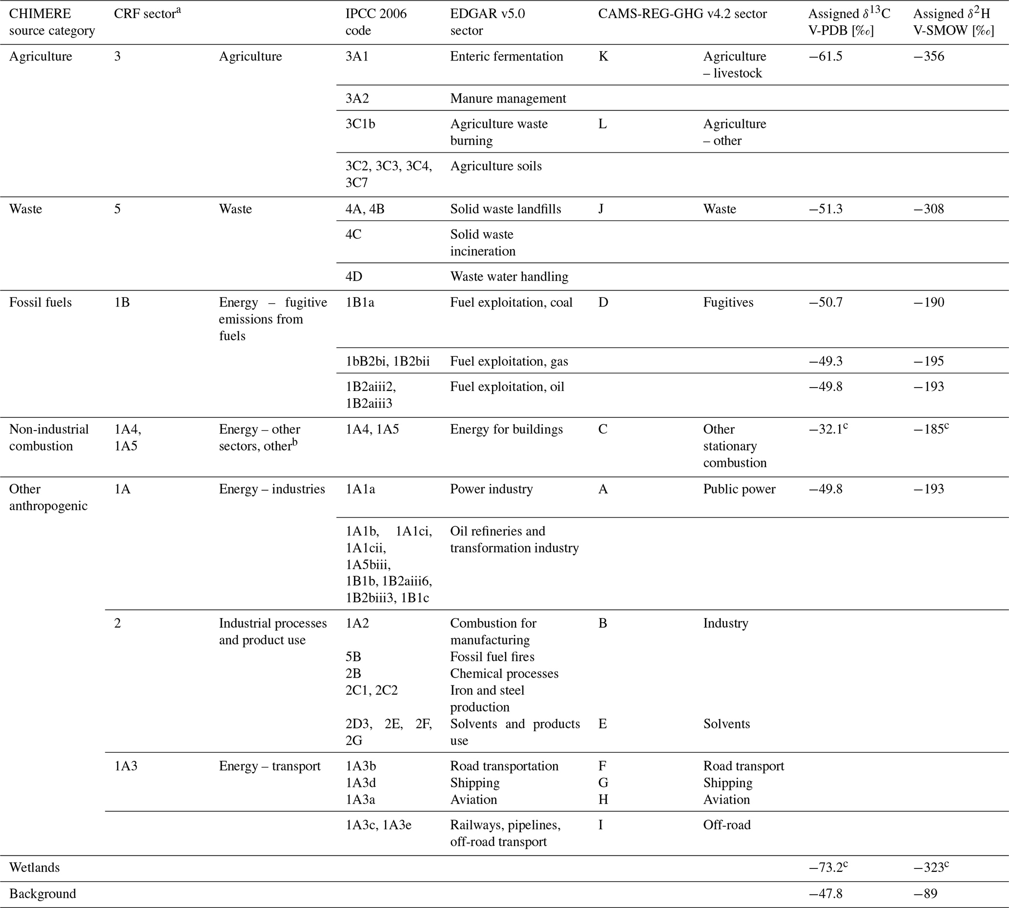
^a European Environment Agency (2019). ^b Mostly the use of coal for heating households (European Environment Agency, 2019). ^c Menoud et al. (2020a, b).

2.5 Modelling

Time series of δ¹³C–CH₄ and δ²H–CH₄ were generated from simulated CH₄ mole fractions using the CHIMERE atmospheric transport model (Menut et al., 2013; Mailler et al., 2017), driven by the PYVAR system (Fortems-Cheiney et al., 2019). CHIMERE is a three-dimensional Eulerian limited-area chemistry-transport model for the simulation of regional atmospheric concentrations of gas-phase and aerosol species.

The simulations were carried out at a horizontal resolution of $\mathrm{0.1}{}^{\circ }\times \mathrm{0.1}{}^{\circ }$ in a domain covering Poland and nearby countries, [46.0–55.9^∘] in latitude and [12.0–25.9^∘] in longitude. The meteorological data used to drive CHIMERE were obtained from the European Centre for Medium-Range Weather Forecast (ECMWF) operational forecast product. The boundary and initial concentrations of χ(CH₄) were taken from the analysis and forecasting system developed in the Monitoring Atmospheric Composition and Climate (MACC) project (Marécal, 2015). They were used to derive the background CH₄ mole fractions.

The CH₄ emission rates over the domain are reported in emission inventories, following a bottom-up approach. We used two anthropogenic emission inventories for this study: EDGAR v5.0 (Emission Database for Global Atmospheric Research; Crippa et al., 2019) and CAMS-REG-GHG v4.2 (Copernicus Atmosphere Monitoring Service REGional inventory for Air Pollutants and GreenHouse Gases; Granier et al., 2012). We classified the emissions in six anthropogenic source categories based on the European Environment Agency (EEA) greenhouse gas inventory common reporting format (CRF, European Environment Agency, 2019). We considered one additional category for natural wetland emissions, which are obtained from the ORCHIDEE-WET process model (Ringeval et al., 2011). The classifications used in CHIMERE and the corresponding categories in the inventories are summarised in Table 1.

The isotopic values at each time t were calculated using the following formula:

$${\mathit{\delta }}_t={\displaystyle \frac{\mathrm{1}}{c_t}}\sum _i^{n_S}(c_{S,i}\cdot {\mathit{\delta }}_{S,i}),$$

with c_t the total mole fraction from the model at time t, c_S the modelled mole fraction attributed to the source S, and δ_S the source signature of each specific source S. In this mass balance, the contribution of the background is treated as a source with assigned isotopic composition. All the assigned source signatures are defined in Table 1.

2.6 Isotopic signatures assigned to CH₄ enhancements

Periods of methane enhancement were identified from the χ(CH₄) time series using a peak extraction method, based on the detection of local maxima from comparison with the neighbouring points. The peaks were selected based on two criteria:

• The peak has a minimal amplitude of 100 ppb.

• The peak is composed of at least three data points, from the maximum to a relative height of 0.6 times the peak height.

In order to define the background more robustly, we included additional data from the 10th lower percentile of χ(CH₄) in a window of ±24 h around the maximum of each peak. The Keeling plot method was thus applied to the data points in the peak, together with the neighbouring background data.

The Keeling plot is a mass balance approach (Keeling, 1961; Pataki et al., 2003), considering the measured CH₄ (m) in ambient air as the sum of a contribution of CH₄ from an emission source (s) and a background (bg) CH₄, such that

$$c_m=c_{\text{bg}}+c_s$$

$$c_m{\mathit{\delta }}_m=c_{\text{bg}}{\mathit{\delta }}_{\text{bg}}+c_s{\mathit{\delta }}_s,$$

with c and δ referring to the mole fraction and isotopic signatures of either ¹³C or ²H, respectively. Rearranging the formula leads to

$${\mathit{\delta }}_m=c_{\text{bg}}\cdot ({\mathit{\delta }}_{\text{bg}}-{\mathit{\delta }}_s)(\mathrm{1}/c_m)+{\mathit{\delta }}_s.$$

We assumed the background mole fraction and isotopic composition to be stable over the time period of each peak. In this case, δ_s is given by the y intercept of the regression line, when plotting δ_m against $\mathrm{1}/c_m$.

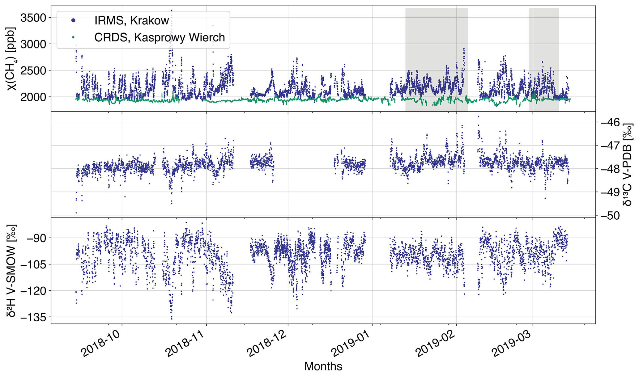
Figure 2 Time series of the observed χ(CH₄) (n=7886), δ¹³C (n=3477), and δ²H (n=4389), together with the χ(CH₄) time series observed at Kasprowy Wierch (green; n=21 028). The shaded areas show when there was a mismatch between the IRMS and CRDS instruments in the mole fractions.

To derive an average source signature for the entire dataset, the Miller–Tans approach was used (Miller and Tans, 2003) because the hypothesis of stable background is violated. This method is based on the following formula:

$$c_m{\mathit{\delta }}_m={\mathit{\delta }}_s{c}_m-c_{\text{bg}}({\mathit{\delta }}_{\text{bg}}-{\mathit{\delta }}_s),$$

where δ_s is now given by the slope of the regression line, when plotting c_m⋅δ_m against c_m.

An isotopic signature was obtained from the linear regressions, and the corresponding uncertainty was derived as 1 standard deviation of the estimated parameter (intercept for the Keeling plot or slope for the Miller–Tans plot). For all Keeling plots, the weighted orthogonal distance regression (ODR) fitting method (Boggs et al., 1992) was used.

The method was applied to both δ¹³C and δ²H measurement results. If two peaks were detected within a 6 h time window in the δ¹³C and δ²H time series, they were considered one single peak and the two signatures were allocated to it. The same method was also used for the modelled χ(CH₄) time series, to allow for the comparison of modelled and measured source signatures.

The Keeling plot method was also used to calculate source isotopic signatures for each location where we sampled CH₄ enhancements during the mobile surveys. The determined source signatures were accepted if they fulfilled at least two of the following criteria for both δ¹³C and δ²H: (i) χ(CH₄) above background >90 ppb, (ii) Pearson's coefficient r² of the linear fit >0.75, and (iii) the standard deviation of the y intercept lower than 5 ‰ for δ¹³C and 100 ‰ for δ²H respectively.

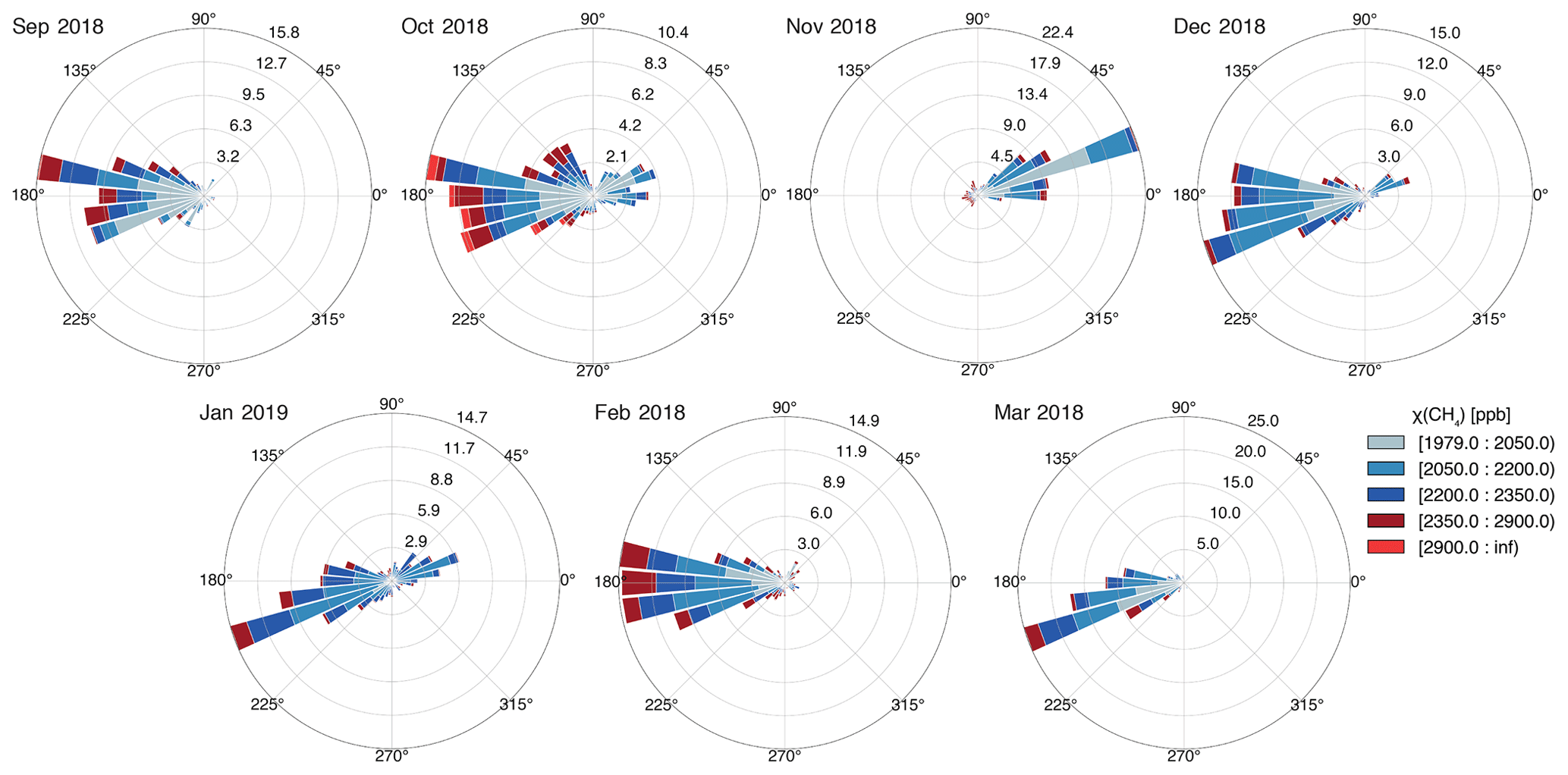
Figure 3 Monthly wind directions during the ambient air measurement period, at the same location. Bar lengths are percentages of records during the specified month (r axis); colours define the χ(CH₄) range (legend).

3 Results and discussion

3.1 Observed time series

The observed time series are shown in Fig. 2, together with measurements of CH₄ at Kasprowy Wierch. We note that in the period February–March 2019, we observed a mismatch of about 80 ppb between the IRMS-derived and simultaneous CRDS χ(CH₄) measurements in the same laboratory (shaded area in Fig. 2). A mismatch in mole fraction can potentially affect the Keeling plot intercepts, and we investigated possible artefacts using various attempts for correction. We realised that the effect of these corrections on the isotopic source signatures is small compared to the observed range (average peak δ¹³C and δ²H changed by 0.1 %; different peak source signatures are shown in Fig. S5b). As no obvious reason for a malfunction of the IRMS instrument could be detected, we decided to use the original data without correction. The peaks in χ(CH₄), compared to the background measured at Kasprowy Wierch, reflect pollution events in Krakow or advected to the measurement site. The maximum χ(CH₄) value was 3634 ppb, measured on 19 October 2018 at 05:30. Simultaneous changes are visible in the δ¹³C and δ²H time series. Increased χ(CH₄) values were always linked with a lower δ²H, but for δ¹³C the measured values could be higher or lower.

The general background threshold is 1986.0 ppb, which corresponds to the 10th lower percentile of the entire dataset. We have found that 70.5 % of the background values (χ(CH₄) <1986.0 ppb) occurred during daytime. The dominant feature in the CH₄ time series is indeed the presence of a diurnal cycle: χ(CH₄) enhancements regularly occurred during the night. This is due to a lowering of the boundary layer when the temperature gradient decreases in the evening. The morning and evening variations in χ(CH₄) were negatively correlated with the temperature data we obtained at the study site. In addition, there were isolated pollution events occurring on top of the night-time accumulation. Between peaks, χ(CH₄) generally went back to a local background level.

The night-time accumulation was particularly visible in the period 14 September to mid-November 2018 and is shown in the Supplement (Fig. S2). Similar night-time enhancements are also visible in the observations of other pollutants such as PM₁₀ at the study location. There was a clear difference in local temperature before and after 15 November 2018: the average air temperature decreased from 12±5.3 to 2.1±4.4 ^∘C and the dew point temperature from 5.3±3.4 to $-\mathrm{3.9}\pm \mathrm{3.4}$ ^∘C until the end of the measurements. The period before mid-November will be referred to as autumn throughout the paper.

The wind directions at the study site were combined with the CH₄ measurement data in Fig. 3 and with wind speeds in Fig. S3. The spread of the wind directions was similar for most of the months: mainly from the west (70 %), with a small contribution (27 %) from the east/north-east. An exception was November 2018, when most of the wind was from the east/north-east direction. March 2019 was characterised by winds from the west only and at particularly strong speeds (on average 3.1 m s⁻¹, compared to 1.8 m s⁻¹ for the other months; Fig. S3). The average CH₄ diurnal cycle, defined as the prominence of night peaks, was on average 334 ppb throughout the entire time period but only 195 ppb when the winds were >2.5 m s⁻¹. This decrease in amplitude with higher wind speeds was not influenced by the direction of the wind. During fall, 84 % of the peaks were observed at night and associated with low wind speeds, which suggests the influence of local pollution sources and a relatively low influence of the wind direction.

The average isotopic values of the background were ${\mathit{\delta }}^{\mathrm{13}}\mathrm{C}=-\mathrm{47.8}\pm \mathrm{0.1}$ ‰ and ${\mathit{\delta }}^{\mathrm{2}}\mathrm{H}=-\mathrm{89}\pm \mathrm{3}$ ‰. The CH₄ enhancements were associated with consistently more negative δ²H but varying δ¹³C. This indicates that the sources were sometimes higher in δ¹³C compared to the ambient CH₄ (i.e. ${\mathit{\delta }}^{\mathrm{13}}\mathrm{C}>-\mathrm{47.8}$ ‰). In contrast, all CH₄ enhancements were associated with lower δ²H during the entire time period.

Figure 4 Time series of the observed (blue circles) and modelled χ(CH₄), δ¹³C and δ²H, based on the EDGAR v5.0 (red) and CAMS-REG-GHG v4.2 (green) inventories.

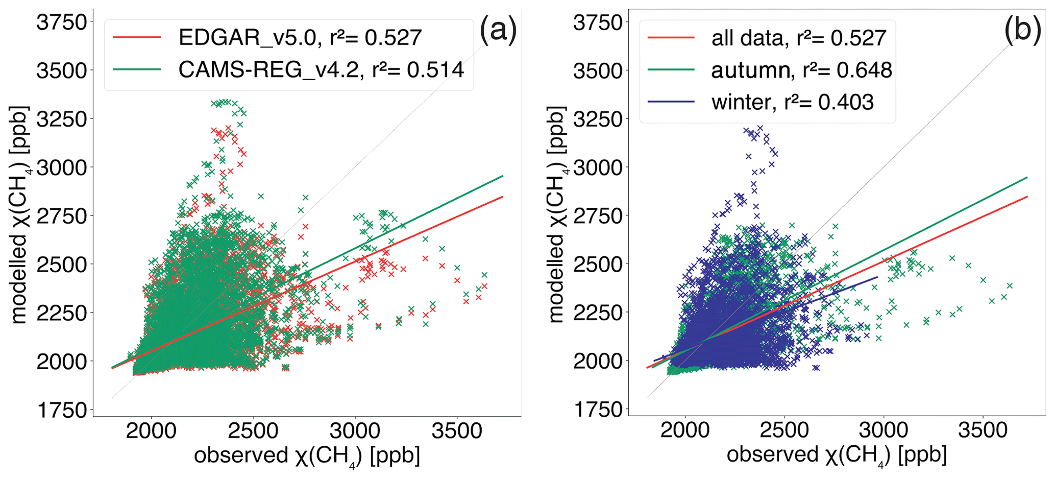
Figure 5 Correlation between observed and modelled χ(CH₄) values, using (a) the EDGAR v5.0 (red) or the CAMS-REG-GHG v4.2 (green) inventories and (b) different time periods: autumn (14 September to 15 November 2018; green) or winter (15 November 2018 to 15 March 2019; blue) computed using EDGAR v5.0.

3.2 Modelled time series

The CH₄ time series obtained with CHIMERE for the grid cell containing the observation site are shown in Fig. 4. We first compared the CH₄ mole fractions measured at Krakow and modelled by CHIMERE in Fig. 5. They show a poor correlation (Pearson's correlation coefficients r²=0.527 and r²=0.514, for model calculations using the EDGAR v5.0 and CAMS-REG-GHG v4.2 inventories, respectively; Fig. 5a). The model globally underestimates the measured χ(CH₄) significantly, with a root mean square error (RMSE) of 164.4 and 173.4 ppb for EDGAR and CAMS, respectively. Yet we see that modelled χ(CH₄) can sometimes be larger than the observations, which is usually due to a shift in the timing of a pollution event (Fig. 4). The wind data used in the model are generally in good agreement with the wind measurements at the study site, but small discrepancies can partly explain the differences in the timing of the peaks. The time series are best reproduced during autumn 2018, using EDGAR v5.0 (r²=0.648; Fig. 5b). As mentioned in Sect. 3.1, autumn 2018 shows a more regular pattern of night-time enhancements of relatively similar amplitudes compared to the winter period. This is better reproduced by the model (Fig. 4). However, the two highest χ(CH₄) measurements were observed in this period (18 October, and 3 November 2018) and were not modelled to the same level (points on the lower right, Fig. 5b). These events largely contribute to the general model underestimation when only considering the autumn data.

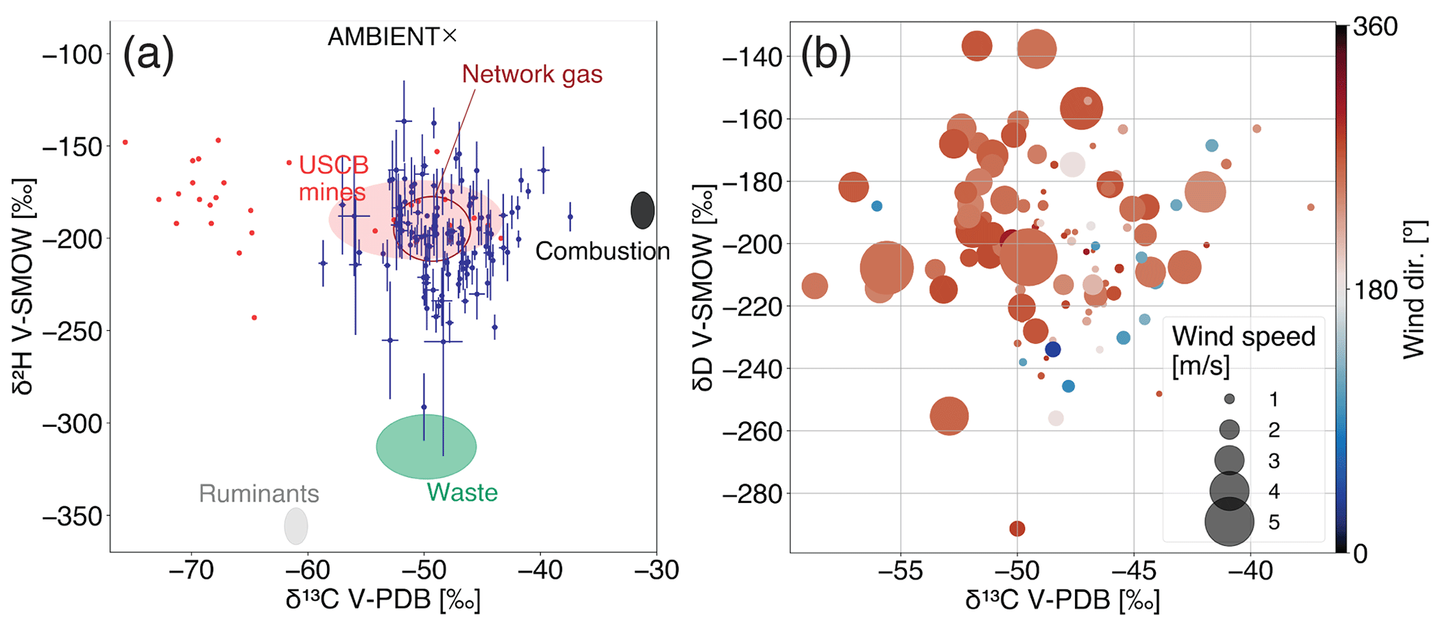
Figure 6 Dual isotope plots of the resulting source signatures from the CH₄ peaks identified in the time series. (a) Dark blue: source signatures with their associated 1σ uncertainties. Coloured areas: ranges of source signatures obtained from the collected samples. If based on one location (ruminants and combustion), the size of the ellipse is 1 order of magnitude of the precision of our isotopic measurements. Red dots: source signatures of USCB coal gas derived from Kotarba (2001), Kotarba and Pluta (2009), and Kedzior et al. (2013). The combustion source signature is from coal waste burning samples reported in Menoud et al. (2020a). (b) Source signatures labelled by the average wind direction (colour) and speed (size) measured during the pollution event.

In winter, the χ(CH₄) enhancements were less regular, with a less consistent diurnal cycle (Fig. S2). The mismatch in the timing of pollution events caused an overestimation by the model (points on the upper left, Fig. 5b). The general slope is still lower than 1, and the fit is worse than during fall. There is a general underestimation of the CH₄ mole fractions at Krakow by the model. This could be explained by the model time series being hourly averages, compared to the observations of sampled air. To account for this bias, we compared the model data with observations that are also averaged over a 1 h window and/or interpolated to the modelled times. This had no effect on the correlation coefficients, suggesting a minor impact of the temporal representation error. Another reason for the underestimation of χ(CH₄) in CHIMERE could be the presence of potential CH₄ sources in the close surroundings of the laboratory. Such emissions could affect the measurements but not the model, where they are diluted over the 11 km grid cell. The misfit between modelled and observed χ(CH₄) could also be due to some errors in the transport modelling or insufficient emissions in the inventories. Szénási (2020) identified the emission inventories as the main source of discrepancies between CHIMERE results and measured time series at two other European locations. The implications on the two inventories are discussed in detail in Sect. 3.4.

Time series of δ¹³C and δ²H in CH₄ show negative or positive excursions relative to the background and are linked to χ(CH₄) peaks (Fig. 4). When using CAMS-REG-GHG v4.2, δ¹³C and δ²H are always negatively correlated with χ(CH₄). But when using the EDGAR v5.0 inventory, δ¹³C values are closer to the background. The isotopic discrepancies will be analysed in detail in relation to the source partitioning in the inventories and the signatures we assigned to each source in Sect. 3.4.

Table 2 Isotope signatures of the different sources sampled in the region surrounding the study site. The values were used as input in the CHIMERE model.

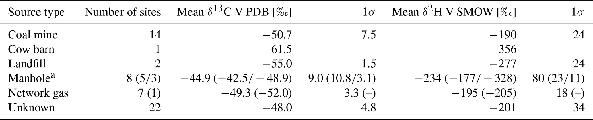
^a Any hole in a road covered by a metal plate that can usually be removed.

3.3 Isotopic source signatures

A total of 126 and 157 peaks were identified in the δ¹³C and δ²H time series, respectively, and 114 peaks were measured commonly by both isotope lines. From the Keeling plot applied to each of the peaks, we obtained the source signatures of the corresponding accumulation events. They can be compared with the determined isotope signatures of the sources sampled in the surrounding area (Fig. 6a).

3.3.1 Isotopic characterisation of the surrounding sources during mobile surveys

The results from 55 individual sites are presented in Table 2 and shown in detail in the Supplement (Table S1 in the Supplement and Fig. S5a). The maximal χ(CH₄) sampled at each location varied between 93 ppb above background and 95 % (pure gas), with a median of 1480 ppb above background. The derived isotopic signatures are in good agreement with the ranges defined for the different categories in the literature (Sherwood et al., 2017). Biogenic sources (a landfill, three manholes, and a cow barn) correspond to the acetate fermentation pathway, characterised by relatively depleted δ¹³C ($<-\mathrm{50}$ ‰) and δ²H ($<-$275 ‰; Milkov and Etiope, 2018). The landfill CH₄ is isotopically more enriched than the cow barn. This can be due to an isotope fractionation from diffusion and oxidation in the soil layers (De Visscher, 2004; Bakkaloglu et al., 2021). The fossil fuel CH₄ emissions we sampled were from coal exploitation and use of natural gas. The natural gas distribution network was sampled outside of compressor stations, close to gas stations and supply valves in residential areas. The results ranged between [−52.3, −44.4] ‰ for δ¹³C and [−225, −177] ‰ for δ²H. To check for temporal variations, four plumes were sampled at an interval of 6 weeks, on 5 February and 19 March 2019. The δ¹³C results were about 4.7 ‰ more depleted, and the δ²H results were 27 ‰ more depleted in March compared to February. One sample was directly taken from the gas supply pipe at the AGH lab in March 2019. The pure gas was 3.6 ‰ and 14 ‰ more depleted in δ¹³C and δ²H, respectively, than the average from accidental leaks (signature in brackets in Table 2), which indicates that the isotopic composition of the city gas in March is relatively depleted compared to February. The network gas composition can change in time because the proportions of gas from several origins vary. Gas migrating in the distribution network can undergo secondary processes. For example CH₄ oxidation into CO₂ influences the isotopic signatures, usually towards more enriched values. Isotopic variations among network gas leaks were also observed previously in other cities (Zazzeri et al., 2017; Maazallahi et al., 2020; Defratyka et al., 2021). The isotopic signature of the pure gas we sampled still falls in the same range as the sampled leaks.

CH₄ emissions from manholes were often observed in the Krakow urban area. The resulting isotopic signatures do not indicate one clear origin and were divided in two groups with distinct δ²H (Table 2). While the isotopically depleted signatures observed at three locations likely come from the sewage system, with a ${\mathit{\delta }}^{\mathrm{2}}\mathrm{H}<-\mathrm{300}$ ‰, the five others contain CH₄ with particularly enriched δ²H (between −202 ‰ and −146 ‰), not typical of microbial fermentation processes (Fig. S5a). We hypothesise that this indicates leakage of natural gas from the distribution pipes to the sewage network, which is sometimes further oxidised, leading to even more enriched isotope signatures.

For most emission plumes, we could not visually identify an obvious CH₄ source. The isotopic signatures of these “unknown” sources range from −58.2 ‰ to −34.9 ‰ V-PDB for δ¹³C and from −285 ‰ to −142 ‰ V-SMOW for δ²H. These large ranges in δ¹³C and δ²H indicated the presence of both fossil fuel and biogenic sources. The average δ²H is >200 ‰, suggesting a major influence from fossil fuel sources. The δ¹³C is in good agreement with the signature found for natural gas (Table 2 and Fig. S5a), and since most of these locations were close to roads and urban settlements, it is likely that they were natural gas leaks.

The isotope signatures from coal mine ventilation shafts and residential gas leaks sampled in this study fall in the same range (Table 2 and Fig. 6a): δ¹³C between −59.8 ‰ and −28.1 ‰ V-PDB and δ²H between −254 ‰ and −152 ‰ V-SMOW, although coal CH₄ has a wider isotopic range. Values of δ¹³C $<-$60 ‰ reported in the literature (Kotarba, 2001; Kotarba and Pluta, 2009; Kedzior et al., 2013; Fig. S5a) confirmed the presence of microbial gas in the USCB. Most δ¹³C values from coal mines in this study were between −58 ‰ and −45 ‰, which also indicates a contribution from microbial gas sources, although in our measurements all δ¹³C signatures from time series peaks and sampled shafts were $>-$60 ‰. Some of the locations sampled in by Kotarba (2001) were revisited in this study. However, their method used direct sampling of CH₄ from different coal layers, aiming at representing the variety in the origin of the gas reservoirs. Our approach was to sample outside the shafts, to obtain the isotopic signature of CH₄ emissions from these shafts to the atmosphere. The very depleted δ¹³C values obtained in these previous studies confirm the presence of purely microbial gas reservoirs in the USCB coal deposits, but our results show that thermogenic gas represents a larger part of the fugitive emissions from mining activities in this area than indicated by Kotarba (2001; Fig. 6a). The heterogeneity of isotopic signatures from coal mining activities in the USCB reflects the geological complexity of the area. Secondary processes (desorption, diffusion or oxidation) also influence the CH₄ isotopic composition and depend on external parameters such as physical characteristics of the coal reservoirs and the soil layers (Niemann and Whiticar, 2017). These represent additional difficulties which have to be taken into account in the isotopic characterisation of coal-associated CH₄ emissions.

The δ²H signatures allow us to identify the CH₄ emissions from microbial fermentation: values below −250 ‰ are indicative of the anaerobic fermentation pathway, such as in the rumen of cows or during waste degradation. Except for one shaft with ${\mathit{\delta }}^{\mathrm{2}}\mathrm{H}=-\mathrm{254}\pm \mathrm{1}$ ‰ (possibly very early mature thermogenic gas in deep formations or a late stage of biodegradation if close to the surface; Milkov and Etiope, 2018), both literature data and our sampled shafts have a δ²H $>-\mathrm{250}$ ‰. This is also true for emissions from the natural gas network, confirming their fossil fuel origin. In the USCB region, δ²H signatures seem to be more suitable than δ¹³C values for source apportionment, similar to recent studies made in European cities (in Hamburg by Maazallahi et al., 2020, and in Bucharest by Fernandez et al., 2021).

3.3.2 Isotopic characterisation of CH₄ in ambient air

The isotopic signatures of the CH₄ pollution events observed in Krakow during the study period are shown in Fig. 6. δ¹³C varied between −59.3 ‰ and −37.4 ‰ V-PDB and δ²H between −291 ‰ and −137 ‰ V-SMOW. As mentioned above, the observed δ¹³C either increased or decreased with higher χ(CH₄), indicating source signatures either lower or higher than the background value. Yet δ¹³C signatures stayed within ±8 ‰ from the background, thus never reaching extreme values. There was 40.5 % of CH₄ peaks with a δ¹³C more enriched than the background of −47.8 ‰. In contrast, the observed δ²H values were always more depleted than ambient. The overall source signatures resulting from the Miller–Tans analysis using all the data points were ${\mathit{\delta }}^{\mathrm{13}}\mathrm{C}=-\mathrm{48.7}\pm \mathrm{0.0}$ ‰ and ${\mathit{\delta }}^{\mathrm{2}}\mathrm{H}=-\mathrm{205}\pm \mathrm{0}$ ‰ (Fig. S4). The comparison with typical signatures of the different CH₄ formation processes indicates that most of these events were from thermogenic sources (Fig. S5b). When compared with isotope signatures of the surrounding sources (Fig. 6a), the source signatures from the long-term time series match the range of coal mine and natural gas emissions the best. Figure 6b shows that most pollution events associated with strong winds fall in the range of more depleted δ¹³C signatures. They were also all advected from west of Krakow, where the USCB is located (Fig. 1). In fact, the δ²H signatures exclude a large contribution from potential biogenic sources and point towards the emissions from coal mines in Silesia. CH₄ sources with the most enriched δ¹³C mostly originated from the east, where the city centre and industrial areas are (Fig. 6b). The Miller–Tans plots were also applied on the time series divided per wind sector (north-east, south-east, south-west, and north-west; Fig. S4). The δ¹³C source signature from north-east is more enriched compared to the other directions, with a value of $-\mathrm{46.3}\pm \mathrm{0.3}$ ‰, and confirms the relative enrichment in δ¹³C of CH₄ sources east of the study site.

In Röckmann et al. (2016) and Menoud et al. (2020b), CH₄ mole fractions, and δ¹³C and δ²H isotopic signatures in ambient air were measured at two locations in the Netherlands. The time series covered 5 months in 2014–2015 and 2016–2017, at Cabauw and Lutjewad, respectively. The average isotopic signatures were $-\mathrm{60.8}\pm \mathrm{0.2}$ ‰ and $-\mathrm{298}\pm \mathrm{1}$ ‰ at Cabauw and $-\mathrm{59.5}\pm \mathrm{0.1}$ ‰ and $-\mathrm{287}\pm \mathrm{1}$ ‰ at Lutjewad, for δ¹³C and δ²H respectively. The main sources contributing to the CH₄ emissions in the Netherlands are cattle farming and waste management. These are biogenic sources, with isotopic signatures representative of the microbial fermentation origin. CH₄ of fossil fuel origin had a minor contribution there, which contrasts a lot with the results from Krakow. Such drastic differences in the isotopic signals of the same trace gas show how a region-specific analysis is crucial to effectively constraining atmospheric emissions.

In Fig. 7, the results of CH₄ mole fraction, peak source signatures, and wind speed and direction are shown in more detail for 8 d in November 2018 and 7 d in February 2019, together with model results using EDGAR v5.0. As mentioned previously, eastern winds generally advected CH₄ with a relatively enriched δ¹³C: 60 % were higher than the background δ¹³C, and all but one were $>-\mathrm{50}$ ‰ V-PDB. In November, the wind was mostly coming from the east (Fig. 3), but enhancements were observed at low wind speed (Fig. 7a, peaks 4 to 7). These pollution events reflect the general signature of the CH₄ emitted in the Krakow urban area and are unlikely to come from coal mines. In Fig. 7a, the modelled peaks C, D, E, and G show a large contribution from the natural gas and from the “other anthropogenic” category. The latter represents mainly the power generation and transportation sectors, as well as the manufacture, chemical, and metal industries. The main contribution is the energy production from fossil fuels, and we assigned a δ¹³C signature corresponding to fossil fuel CH₄ to this category (Table 1). The modelled results for these peaks are generally similar to the measured ones. The magnitude of the χ(CH₄) enhancements also matches the observations relatively well: modelled peaks C, D, and E were 79, 23, and 14 ppb larger than the observed peaks 3, 4, and 5, respectively. Yet for peak C (observed peak 3), the model δ¹³C signature is 2.8 ‰ lower than the one from the measurements and showed a majority of emissions from “other anthropogenic” sources (37 %). Part of these emissions can be from the incomplete combustion of CH₄, and such combustion-related emissions have a more enriched δ¹³C signature than fossil fuel CH₄ (Fig. 6a). Results from mobile surveys in Paris identified fuel-based residential heating systems as urban CH₄ sources, with a slightly more enriched isotopic composition than the local gas leaks (Defratyka et al., 2021). Therefore, either the proportion of emissions in the “non-industrial combustion” category or the δ¹³C signature assigned to the “other anthropogenic” emission category was underestimated. We note that we could not characterise this source category by sampling. Uncertainties in the assigned signature are unavoidable when a given category is a combination of different sources; not only do the processes have different isotopic signatures, but the contribution from the different sources could change from one pollution event to another. For δ²H, the agreement between observed and modelled signatures for these November night peaks is good. All fossil fuel and pyrogenic δ²H signatures used in this study are relatively close to each other (Table 1) and to the average peak δ²H source signature. Thus, the δ²H signatures do not allow for a distinction between these two processes.

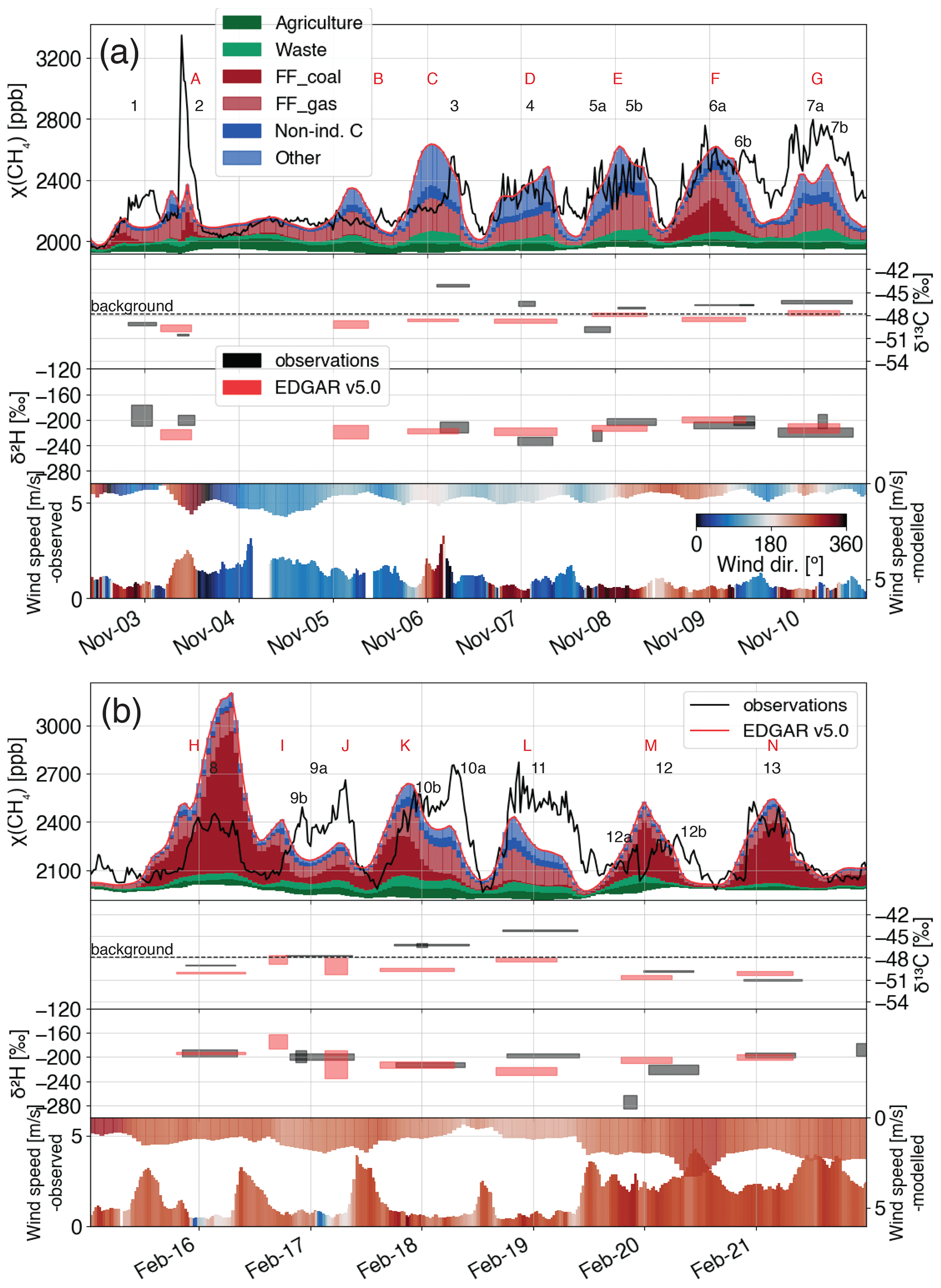
Figure 7 Detailed analysis of two subsets of the dataset: (a) from 2 to 10 November 2018 and (b) from 15 to 22 February 2019. Top panels: observed (grey) and modelled (red) mole fractions and relative source contributions from the EDGAR v5.0 inventory. FF denotes fossil fuel, and non-ind. C denotes non-industrial combustion. Middle panels: δ¹³C and δ²H source signatures of individual peaks of the observed (grey, from peak 1 to 13) and modelled (red, from peak A to N) time series. Box heights represent ±1σ of each peak isotopic signature. Bottom panels: wind speed and direction measured simultaneously at the study site (pointing up) and used for the CHIMERE simulations (pointing down).

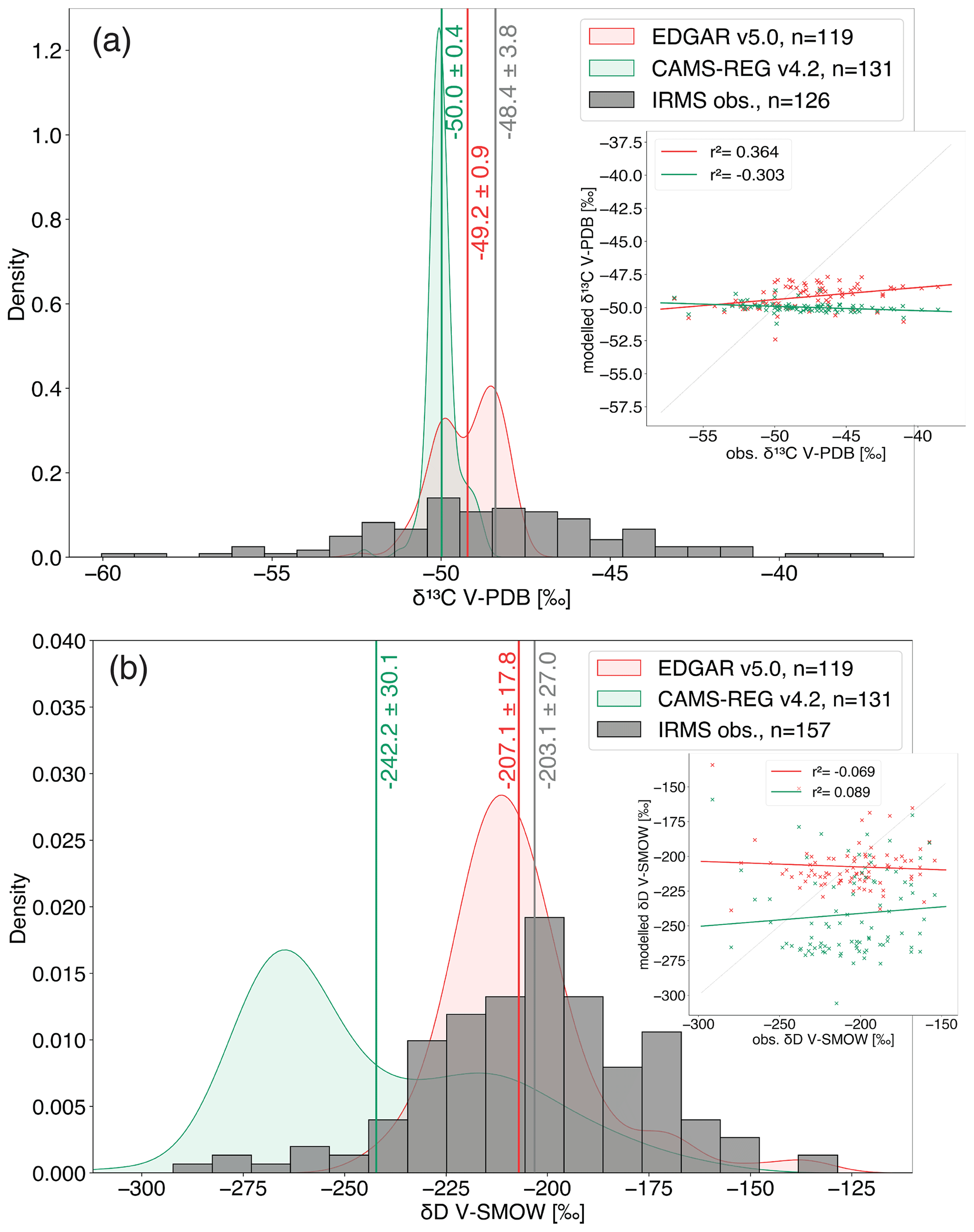
Figure 8 Distribution of source signatures of all peaks and in the inset the correlation between modelled and observed ones. The vertical lines show the average values of each distribution (±1σ). (a) δ¹³C signatures in the observed time series (grey, n=126), modelled using EDGAR v5.0 (red, n=119), and modelled using CAMS-REG-GHG v4.2 (green, n=131) time series. (b) δ²H signatures in the observed time series (grey, n=157), modelled using EDGAR v5.0 (red, n=119), and modelled using CAMS-REG-GHG v4.2 (green, n=131) time series.

Some peaks advected at low wind speeds during the night are also visible in Fig. 7b (peaks 9 to 11) and show similarly enriched δ¹³C signatures. The wind direction was different for these night peaks between February and November, but the low wind speeds again indicate that this represents the local emission mix. The model time series showed peaks that occurred simultaneously to the measured ones (K and L in Fig. 7b) although with different χ(CH₄) maxima than the measurements (−115, −339, and +203 ppb, respectively). For peaks K and L, the source partitioning from the inventory is similar to the other night peaks shown in Fig. 7a. The δ¹³C signatures of these urban emissions are however underestimated in the model and so are the CH₄ mole fractions, in particular for peak 11 (corresponding to peak L in the model time series). We suggest that at a close distance east of the study site, the share of emissions from the combustion sources is likely underestimated. These additional emissions could be from residential heating or the energy production sector. The δ²H signature of peak 11 (L) also differs significantly between the model and measurements. This further indicates that the missing CH₄ emissions must be mostly combustion-related because of the relatively enriched δ¹³C and δ²H we observed ($-\mathrm{44.2}\pm \mathrm{0.1}$ ‰ V-PDB and $-\mathrm{198}\pm \mathrm{3}$ ‰ V-SMOW, respectively, for peak 11).

Table 3 Methane absolute emissions and contributions of the different source categories used in CHIMERE to the total simulated χ(CH₄), for the EDGAR v5.0 and CAMS-REG-GHG v4.2 inventories.

The δ¹³C signatures shifted towards being more depleted in heavy isotopes values after 19 February. δ¹³C went from $-\mathrm{44.2}\pm \mathrm{0.1}$ ‰ for peak 11 to $-\mathrm{49.8}\pm \mathrm{0.1}$ ‰ for peak 13. Peaks 12 and 13 (respectively M and N in the model) were advected by strong westerly winds. The share of coal-related emissions reported in the inventory increased from peak M compared to peaks K and L and is supported by the decrease in δ¹³C, also in the modelled signatures. This confirms a source shift from urban to coal activities further west of Krakow from 19 February 2019. Whenever the EDGAR inventory reported large contributions from coal mine emissions, such as for peaks F, H, K, M, and N (corresponding to 6a, 8, 10a, 12, and 13, respectively), the model wind direction corresponds to the USCB. The associated isotopic signatures were in relatively good agreement for peaks H, M, and N, where coal emissions represented >50 % of the total. Small discrepancies (within 3 ‰ in δ¹³C) are explained by the heterogeneity of isotopic signatures from the different mine shafts. This confirms that the average isotopic signatures for this category are well characterised in this study. For peaks F and K, δ¹³C values are at least 2 ‰ lower than the observations (peaks 6a and 10a). The share of emissions from the USCB are therefore likely overestimated in these two cases.

Seven peaks in the entire dataset showed a ${\mathit{\delta }}^{\mathrm{2}}\mathrm{H}<-\mathrm{255}$ ‰ V-SMOW, suggesting a larger contribution from biogenic sources (Fig. 6a). They are associated with large uncertainties because the peak magnitudes were low. These peaks were not modelled by CHIMERE, using either inventory. They represent isolated pollution events, disconnected from the daily cycle and not particularly related to a certain wind direction. There could be occasionally larger biogenic emissions such as from a waste facility that are advected to the measurement site. In Fig. 7b, a depleted δ²H signature was derived from a small peak (12a). The χ(CH₄) enhancement was not significant in the time series of δ¹³C, which suggests a very short pollution event. It still correlated with a short-term change in wind direction towards a more north/north-west origin. Such abrupt changes are not visible in the model wind data because of its coarser temporal resolution. Based on its clearly biogenic isotopic signal, as well as the wind direction, this event might reflect the contribution from the two large waste treatment facilities located north-west of Krakow (Fig. 1). This needs to be confirmed by observations at higher mole fractions to reduce the uncertainty in the source signature and to be able to derive a signature for δ¹³C, as we are reaching our detection limit here. Further measurements at this location would be useful to specifically characterise this source.

In addition to the night-time accumulations of CH₄, we observed occasional χ(CH₄) peaks during the day, not linked to the night-time lowering of the boundary layer. CH₄ emissions coming from a specific location and advected by strong winds to the measurement site resulted in sharp peaks, such as peak 2 in Fig. 7a, that are separate from the daily cycle. An increase in wind speed (from 0.7 to 2.2 m s⁻¹) and constant wind direction of 251^∘ caused a sharp increase in χ(CH₄) by 1360 ppb, over only 3 h. The peak was reproduced by the model (peak A) but with a lower magnitude, which can be explained by the differences in the wind data. The observed source signatures were ${\mathit{\delta }}^{\mathrm{2}}\mathrm{H}=-\mathrm{190}\pm \mathrm{9}$ ‰, indicating fossil-fuel-related emissions, and ${\mathit{\delta }}^{\mathrm{13}}\mathrm{C}=-\mathrm{49.3}\pm \mathrm{0.5}$ ‰, corresponding to localised coal mine fugitive emissions. The isotope signatures from the model using the EDGAR inventory differ significantly from the observed ones, even though coal extraction is still indicated as the main source. The input source signatures in the model represent all coal-related emissions and therefore might fail in reproducing the signature of emissions at the scale of individual sites.

3.4 CH₄ source partitioning in the inventories linked to isotopic composition

The CH₄ emissions for each source category from the inventories over the studied domain and the simulated CH₄ mole fractions in the grid cell of the measurements' location are presented in Table 3.

The modelled isotopic signatures when using the CAMS-REG-GHG v4.2 inventory show that the CH₄ sources are always more isotopically depleted in δ¹³C than when using EDGAR v5.0 (Sect. 3.2, Fig. 4). When looking at the source partitioning between the two inventories, this can be explained by the much higher contribution from waste emissions when using the CAMS inventory (Table 3). These emissions have a particularly large influence at our study site (43.8 % of total added mole fraction), whereas the share in the emissions is not so large over the entire domain (26.2 % of total emissions). The emissions maps of both inventories are shown in Fig. S6. The higher waste emissions in CAMS-REG-GHG v4.2 are indeed coming from the Silesia region (Fig. S6). There is no evidence of particularly large amounts of domestic waste or waste collection facilities in this area. The Silesia and Krakow regions report comparable amounts of municipal waste per inhabitants and in the same range as other regions of Poland (Statistics Poland, 2018). However, there is 5 times more waste from mining activities reported in Silesia than the other Polish regions (Statistics Poland, 2018). The emissions reported by CAMS are therefore associated with coal mining activities, especially mineral washing in the coal preparation plants. In our approach of distinguishing sources based on their isotopic signature, these emissions should be considered as being fossil-fuel-related. However, in the CAMS inventory they are combined with waste emissions from the fermentation of organic substrate, which have a distinctly depleted isotope signature (Table 2, Fig. 6a). The emissions from on-site energy use for coal mining and for the manufacture of secondary and tertiary products from coal are included in the “other anthropogenic” category in both inventories (CRF sector 1.B.1.c, European Environment Agency, 2019). But in the EDGAR inventory, emissions categorised as being from coal mining include fugitive emissions from the extraction and all the processing steps prior to combustion (CRF sector 1.B.1.a, European Environment Agency, 2019). They were therefore associated with the same signature as the coal extraction itself, which results in a better match with the observations than when using CAMS-REG-GHG v4.2.

The isotopic signatures per peak obtained from the model are compared with the ones from the observations in Fig. 8. The histograms show the distribution of isotopic signatures from the Keeling plots applied to each peak we extracted from the measured and modelled time series. The correlation plots allow the CH₄ peaks detected simultaneously to be compared in the observed and modelled time series. When using the CAMS-REG-GHG v4.2 inventory, the δ¹³C source signatures varied between −52.3 ‰ and −48.7 ‰, a much more narrow range than from −59.3 ‰ to −37.4 ‰ for the observations. This reflects the over-representation of the waste category and its associated depleted δ¹³C signature. This bias towards depleted values is also visible in the δ²H signatures. The source signatures when using the EDGAR v5.0 inventory match the observations better: the average δ¹³C and δ²H of all enhancements agree within their uncertainties, and the δ¹³C signatures are slightly correlated (r²=0.36). The distribution of δ¹³C signatures with EDGAR has a bimodal shape that we also observe in the measured data, but it covers a smaller range of values. Some of the most enriched signatures in the observations are not reproduced by the model, for both δ¹³C and δ²H (Fig. 8). As shown in Fig. 6a, δ²H allows microbial fermentation to be distinguished from fossil fuel (or pyrogenic) sources, whereas the δ¹³C ranges for these two source types overlap. This suggests that the fossil fuel fugitive and combustion-related emissions in the inventories are underestimated. This mismatch is consistent with the lower χ(CH₄) in the model compared to the observations (Fig. 5) and is supported by our findings on the emission peak signatures (Fig. 7).

Finally, the absence of correlation between δ²H signatures from the model and observations (Fig. 8b) emphasises the need for more δ²H measurements in order to more precisely constrain the sources for this isotope signature. This limits the conclusions we could derive from measurements of δ²H, especially in the context where δ²H is particularly relevant for source attribution.

4 Conclusions

This study presents measurements of CH₄ mole fractions and δ¹³C and δ²H of CH₄ in ambient air, performed continuously during 6 months in 2018–2019 at Krakow, Poland. The results were combined with model simulations from a high-resolution regional transport model based on two different emission inventories.

The source signatures of the pollution events observed in Krakow were compared with signatures from sources sampled around the study area. This allows us to identify the fossil fuel-related sources as the main contributor to the CH₄ emissions. The wind directions pointed towards Silesian coal mines, but the use of natural gas in the urban area of Krakow is also an important source. Our results showed that despite the presence of microbial CH₄ reservoirs, CH₄ of thermogenic origin contributes the most to the atmospheric emissions from the USCB mine shafts. Despite their variability, the CH₄ isotopic signatures of Silesian coal mines are generally well constrained and the overall emissions well characterised. The δ¹³C source signature assigned to the USCB CH₄ emissions (−50.7 ‰ V-PDB) agreed with the most recent estimate of −50.9 ‰ V-PDB by Gałkowski et al. (2020) (2020). However, the δ²H source signatures were well reproduced when using a higher input δ²H for coal mining emissions (−190 ‰ instead of −225 ‰ V-SMOW). This study significantly helps to constrain the CH₄ isotopic signatures from the USCB coal mining activities. Our isotopic observations when the wind was from the west at relatively high speeds confirm the prominence of coal-related CH₄ emissions compared to biogenic ones (agriculture and waste). The main limitation of our approach in the context of Krakow is due to the overlap between the isotopic signatures from coal mines and natural gas but could partly be overcome by a detailed analysis of the wind data.

In comparison to measurements made in the Netherlands (Röckmann et al., 2016; Menoud et al., 2020b), the range of CH₄ isotopic signatures derived from the Krakow measurements was more enriched in δ¹³C and δ²H, by 10 ‰ and 100 ‰, respectively. These large differences are directly related to the heterogeneity in the human activities impacting our climate: from agriculture (especially cattle farming) in the central Netherlands to the exploitation of fossil fuels in south-western Poland. This provides additional evidence for the value that the analysis of isotopologues can have in constraining the local to regional methane budget. Emission inventories would generally benefit from similar measurements at other locations, mostly where several types of CH₄ sources are present. With the CH₄ isotopic composition measured continuously, we can identify under- or overestimated sources or detect new sources.

The χ(CH₄) computed using both inventories matched the measurements relatively well (r²=0.65 using EDGAR v5.0) during autumn 2018. However, the agreement is less during the winter months (r²=0.40), largely reflecting discrepancies in the timing of the pollution events. The model also underestimated the CH₄ levels by on average 170 ppb compared to the observations. The isotopic results suggest that increased emissions in the inventories must be of fossil fuel origin.

The average isotopic source signatures from the model using the EDGAR v5.0 inventory were in good agreement with the ones from the measurements, which confirms the predominance of fossil fuel emissions. Larger differences were observed on the level of individual peaks. Uncertainties remain because of the combination of different sources within one category in the EDGAR v5.0 inventory. Small discrepancies between observed and modelled signatures are also due to the inherent diversity of isotopic signatures, even within one source category, like we observed when sampling the USCB mines. When multiple CH₄ sources contribute to the total χ(CH₄), as was the case for the Krakow urban area, the uncertainties in the isotopic characterisation increase further. The CAMS-REG-GHG v4.2 inventory quantified waste emissions as the main contributor to the regional CH₄ emissions but does not distinguish residential waste from waste associated with the processing of coal, which resulted in a large bias towards isotopically depleted sources. Therefore, our method fails to assess in detail the performance of this inventory. Nevertheless we show the power of continuous isotope data for analysing CH₄ emission sources on monthly and daily scales, in a very detailed manner. Continuous measurements at fixed locations can be used in future work to improve and validate inventories and thus help target the mitigation of the right sources. It requires CH₄ sources to be characterised locally, and additional sampling campaigns in the city of Krakow would be required to better define the different sources and their isotopic composition, especially to target CH₄ emissions with enriched δ¹³C ($>-\mathrm{45}$ ‰).

Using δ²H measurements in the identification of the sources was essential in this region, compared to δ¹³C, as the δ¹³C from coal mine activities and the network gas overlaps with CH₄ emitted from microbial sources such as waste. Yet our conclusions using δ²H isotopes are restricted by the limited number of δ²H measurements available. We show that the use of δ²H data for CH₄ source appointment is not to be neglected and might help to characterise emissions at other locations, especially in the presence of fossil fuel CH₄ of microbial origin. In this case, the relatively depleted δ¹³C would overlap with the δ¹³C signatures from microbial fermentation sources (mainly ruminants, waste, wetlands), as for example in the case of the Surat Basin (Australian) coal deposits (Lu et al., 2021).

Our δ¹³C data generally support the recent re-evaluation of global δ¹³C–CH₄ from fossil fuel sources towards less enriched values (Schwietzke et al., 2016). The data presented here were collected in an area that has been under-investigated in the past, compared to its importance for the European CH₄ emissions. It is therefore an important contribution to studies on the global CH₄ budget. The high time resolution and temporal coverage of χ(CH₄), δ¹³C, and δ²H in CH₄ provided by these data are also particularly helpful to evaluate transport models on regional and global scales.