Assessing urban methane emissions using column-observing portable Fourier transform infrared (FTIR) spectrometers and a novel Bayesian inversion framework

Cities represent a large and concentrated portion of global greenhouse gas emissions, including methane. Quantifying methane emissions from urban areas is difficult, and inventories made using bottom-up accounting methods often differ greatly from top-down estimates generated from atmospheric observations. Emissions from leaks in natural gas infrastructure are difficult to predict and are therefore poorly constrained in bottom-up inventories. Natural gas infrastructure leaks and emissions from end uses can be spread throughout the city, and this diffuse source can represent a significant fraction of a city's total emissions.

We investigated diffuse methane emissions of the city of Indianapolis, USA, during a field campaign in May 2016. A network of five portable solar-tracking Fourier transform infrared (FTIR) spectrometers was deployed throughout the city. These instruments measure the mole fraction of methane in a total column of air, giving them sensitivity to larger areas of the city than in situ sensors at the surface.

We present an innovative inversion method to link these total column concentrations to surface fluxes. This method combines a Lagrangian transport model with a Bayesian inversion framework to estimate surface emissions and their uncertainties, together with determining the concentrations of methane in the air flowing into the city. Variations exceeding 10 ppb were observed in the inflowing air on a typical day, which is somewhat larger than the enhancements due to urban emissions (<5 ppb downwind of the city). We found diffuse methane emissions of 73(±22) mol s⁻¹, which is about 50 % of the urban total and 68 % higher than estimated from bottom-up methods, although it is somewhat smaller than estimates from studies using tower and aircraft observations. The measurement and model techniques developed here address many of the challenges present when quantifying urban greenhouse gas emissions and will help in the design of future measurement schemes in other cities.

1 Introduction

Methane (CH₄) is a powerful greenhouse gas that is emitted to the atmosphere from both anthropogenic and natural sources (Montzka et al., 2011). Urban areas, which represent the majority of global anthropogenic greenhouse gas emissions (Hopkins et al., 2016), contain a mix of sources of methane, including landfills, industrial facilities, and fugitive emissions associated with natural gas infrastructure and end use. These fugitive emissions are a significant source of methane in some cities (Townsend-Small et al., 2012; McKain et al., 2015; Chen et al., 2020), but their detection and quantification are difficult (Phillips et al., 2013; Brandt et al., 2014). Governments have established goals for mitigating these emissions (Rosenzweig et al., 2010), creating a need for long-term measurement systems to monitor progress and identify areas where action is needed (Gurney et al., 2015; Dietrich et al., 2021).

The relative contribution of these different types of sources can vary greatly from city to city. In the greater Boston region, one study concluded that 60 % to 100 % of methane emissions were due to leaks and inefficiencies in the natural gas sector. It was estimated that Boston's natural gas system had an overall emission rate of 2.1 % to 3.3 % of gas used in the region, which is much larger than a published national estimate of 1.1 %. It was thought that these large emissions were likely attributable to aging cast iron and bare steel pipelines (McKain et al., 2015). A contrasting example would be the emissions profile of Indianapolis, Indiana, where only 24 km out of 6521 km of pipelines are cast iron, with the vast majority being newer plastic and protected steel (Lamb et al., 2016; Von Fischer et al., 2017). Indianapolis also has large point sources in the city, such as landfills, which result in an estimated natural gas sector contribution ranging from 21 % to 69 % of total urban emissions (Cambaliza et al., 2015; Lamb et al., 2016; Maasakkers et al., 2016; Balashov et al., 2020). Even in cities with modern infrastructure, diffuse emissions can still be a large percentage of the total urban methane budget, and accurate information about their magnitude is critical for those interested in mitigating the problem.

There are two basic methods to quantify the emission rate of a trace gas (such as methane) from an urban area. The first is the bottom-up approach, which starts by taking an inventory of the major point sources (e.g., landfills, compressor stations) and density of diffuse sources in the domain and then applying emission factors to all of these sources to compute a total flux value. We consider any source with a known extent less than 1 km × 1 km (one grid cell in our model) to be a point source. Examples of bottom-up methane inventories available for the continental United States include EDGAR (European Commission, 2011) and the EPA gridded national inventory (Maasakkers et al., 2016).

The other approach to the quantification of emissions is the top-down method, whereby atmospheric measurements are made and the emission rate is derived from these observations. Top-down methods that have been successfully used to constrain urban methane emissions include aircraft mass-balance techniques (Cambaliza et al., 2015) and inverse modeling approaches using in situ sensors mounted on towers (McKain et al., 2015) and/or aircraft (Peischl et al., 2013; Wennberg et al., 2017; Lopez-Coto et al., 2020). Currently, anthropogenic methane emission estimates from bottom-up and top-down methods can differ greatly at national (Miller et al., 2013) and urban (Lamb et al., 2016) scales, and improved methods in both approaches are needed in order to provide urban planners and lawmakers with the information they need to enact effective carbon policies (Duren and Miller, 2012). The goal of this paper is to quantify diffuse methane emissions from an urban area with improved natural gas infrastructure (Indianapolis) on a city-wide scale using a small network of total column sensors. We focus on diffuse emissions here because these have been proven to be the most difficult to quantify, and the major point sources in Indianapolis are few and relatively well characterized. In order to accomplish this, solutions to several measurement and modeling challenges must be devised. These challenges include relatively low signal-to-noise levels and difficulty in determining the background concentration of methane in the air entering the city. A rigorous analysis of the errors involved is also critical to the success of the project.

Satellite observations of methane have been used in inverse modeling estimates of methane emissions (Bergamaschi et al., 2009); however, current generation satellites lack the resolution needed to resolve emissions on urban scales (Turner et al., 2018). Past and current spaceborne methane instruments include SCIAMACHY (Bovensmann et al., 2002) (2003–2012), which was resolved at 30 km × 60 km, and GOSAT (Kuze et al., 2009) (2009–present), which has 10 km diameter pixels. The latest major satellite with methane measurement capabilities, TROPOMI (Veefkind et al., 2012; Hu et al., 2018), is able to resolve 5.6 × 3.5 km pixels across the globe. Several methane-observing satellites with higher spatial resolution are currently being developed (Jacob et al., 2016), but their ability to resolve emissions from cities is unknown, and efforts to quantify urban emissions from space will require extensive calibration and validation with ground-based and aircraft-based measurements.

EM27/SUN spectrometers

The Bruker model EM27/SUN is a compact, solar-tracking total column Fourier transform infrared (FTIR) spectrometer (Gisi et al., 2012; Hase et al., 2016). These instruments record high-resolution solar spectra in a near-infrared window that includes strong absorption features for CO₂, CH₄, CO, H₂O, and O₂. Using retrieval algorithms developed for the Total Column Carbon Observing Network (TCCON, Wunch et al., 2011), the EM27/SUN can be used to compute the total column concentrations of these gases every 6 s during sunlit hours (Chen et al., 2016; Hedelius et al., 2016). The retrieval product is the total column dry-air mole fraction of methane (denoted XCH₄, units of parts per billion), which represents what the mole fraction of methane in the column would be if water vapor was removed. EM27/SUN sensors have been calibrated alongside TCCON instruments, which are themselves calibrated against WMO in situ standards.

Using a surface-based total column sensor offers some advantages over in situ (direct sampling) methods. Since they sample an entire column of air, they do not need to be mounted on towers or tall buildings in order to measure methane aloft, and they are sensitive to emissions from an extended area of the city (Wu et al., 2018). Hence, the EM27/SUN can be deployed and relocated quickly and inexpensively, while still adequately sampling the desired emission sources. Using multiple EM27/SUNs in an upwind–downwind configuration has been proven to be an effective way to measure methane emissions from dairy farms (Chen et al., 2016; Viatte et al., 2017) and coal-mining areas (Luther et al., 2019), and some work has explored their usefulness in cities (Hase et al., 2015; Chen et al., 2020; Dietrich et al., 2021). There is also a coordinated effort to build a worldwide network of these sensors (Frey et al., 2019). These spectrometers have also been used to make observations of carbon emissions from individual sources such as power plants (Toja-Silva et al., 2017) and volcanoes (Butz et al., 2017). Some work has even been done to take column measurements from moving platforms (Klappenbach et al., 2015; Kille et al., 2017). The sensitivity of these instruments enables them to detect small methane gradients across cities associated with fugitive emissions from natural gas infrastructure. In this paper, a network of sensors was temporarily installed in the city of Indianapolis in order to measure diffuse emissions identified in previous studies (Lamb et al., 2016). Total column sensors measure absorption spectra using the sun as a source and therefore cannot be used at night or in overcast situations, but they can operate well in partly cloudy conditions.

2 Methods

A field campaign in Indianapolis, Indiana, was carried out in May 2016. Methane emissions have already been characterized in Indianapolis by the INFLUX experiment (Lamb et al., 2016; Davis et al., 2017) using several years of in situ measurements from towers as well as aircraft observations. Indianapolis lacks complex terrain and has few large upwind methane point sources, which would make the transport modeling more difficult. Extensive work has also been done to characterize the methane concentrations of inflowing air entering Indianapolis (Balashov et al., 2020).

During the campaign, five EM27/SUN spectrometers (designated ha, hb, kf, ma, and pi) were deployed throughout the city for 5 d of measurement. Four of the sensors were set up in fixed locations throughout the campaign, while one unit (pi) was moved from day to day based on wind forecasts to maximize sensitivity to urban emissions.

2.1 Spatial distribution of fluxes

The largest single source of methane emissions in Indianapolis is the South Side Landfill (SSLF), which emits methane at a rate of 28 to 45 mol s⁻¹ (Cambaliza et al., 2015; Lamb et al., 2016; Maasakkers et al., 2016; Balashov et al., 2020). Three other landfills, which are outside the city limits but inside the domain of this study, are the Twinbridges Landfill (17.5 mol s⁻¹), the Caldwell Landfill (8.5 mol s⁻¹), and the Noblesville Landfill (0.1 mol s⁻¹). The city's main wastewater treatment facility, located near the SSLF, is also a notable methane source, with an estimated emission rate of 3 to 7 mol s⁻¹. Natural gas is supplied to the city via the Panhandle Eastern Pipeline, which runs from Oklahoma to Michigan. The connection point between this pipeline and the municipal pipeline grid is known as the city gate (CG) and is also a potential methane point source. Emissions from the CG are estimated at 1 mol s⁻¹ (Balashov et al., 2020).

Additional sources of methane emissions are leaks in the city's natural gas infrastructure, venting, and inefficiencies in natural gas combustion downstream. These sources are spread throughout the city and referred to as diffuse emissions; they have been estimated to account for an additional 20 to 64 mol s⁻¹, or 21 % to 69 %, of total methane emissions (Lamb et al., 2016). Lamb et al. (2016) modeled the diffuse source on a 1 × 1 km² grid spatially distributed based on HESTIA emissions of CO₂ from natural gas combustion (Gurney et al., 2012). This approach was taken because high-resolution methane inventories are not available and because the location of fugitive emissions could plausibly be correlated with sites of combustion. This distribution is also shown in Fig. 1.

The resulting gridded emissions product, F, is a function of longitude (x), latitude (y), and emissions sector (s). This spatial distribution was used in previous work constraining methane fluxes in Indianapolis using tower-based sensors (Lamb et al., 2016), as shown in Fig. 1 and described in Table 1. Emissions were ultimately grouped into four sectors. We have chosen to define sectors based on the Intergovernmental Panel on Climate Change (IPCC) guidelines (IPCC, 2006). The first three sectors of interest in Indianapolis and their corresponding IPCC abbreviations are diffuse fugitive emissions (1B) , landfills (6A), and wastewater treatment (6B). The fourth sector, the city gate, is abbreviated CG. The city gate also falls into IPCC category 1B but was treated separately for this study as it is a significant point source. Although some works have used EM27/SUN observations to constrain fluxes from point sources (Toja-Silva et al., 2017), the sensors in this experiment were spread across the city to maximize sensitivity to diffuse emissions. The locations of the point sources and sensors are given in Tables 1 and 2 and shown in Fig. 1, which also shows the extent of the study domain.

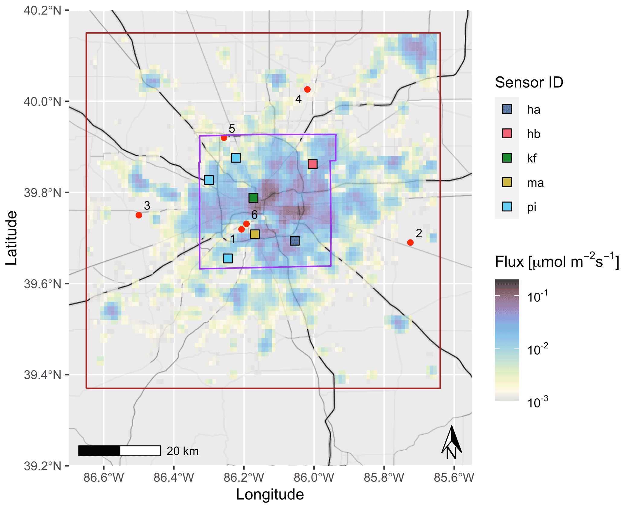
Figure 1 Prior estimate of emissions due to natural gas infrastructure. EM27/SUN deployment locations are shown with squares. Locations of known point sources are also shown (red circles, summarized in Table 1). The study domain is shown in brown, and the boundary of Marion County is shown in purple. Map tiles by Stamen Design under CC BY 3.0. Data by OpenStreetMap; © OpenStreetMap contributors 2020. Distributed under the Open Data Commons Open Database License (ODbL) v1.0.

Table 1 Location and estimated methane flux of major point sources in Indianapolis.

Fluxes are given in moles per second (mol s⁻¹). Adapted from (Lamb et al., 2016).

Table 2 Location of EM27/SUNs on each day of the campaign. All instruments were operated at ground level, except for hb, which was on top of a 20 m building.

2.2 EM27/SUN calibration

Absolute calibrations of EM27/SUN spectrometers have been performed by comparing measurements to co-located TCCON stations (Frey et al., 2019; Hedelius et al., 2016). However, when using a multiple-sensor network, relative calibrations between instruments have proven to be sufficiently precise and to have minimal drift over time (Chen et al., 2016; Frey et al., 2019). To obtain relative calibrations, 2 additional days of data were taken: 1 d before and 1 d after the field deployments. On these calibration days, all five sensors were placed next to each other to ensure that they all measured the same air mass. The relative offset between sensors is stable, and our studies have shown that this type of calibration results in a relative XCH₄ precision between instruments of 0.2 ppb when using an averaging time of 10 min (Chen et al., 2016). The offset calibration data are shown in Fig. 2.

Ahead of the campaign we noted increasing degradation of the solar-tracking mirrors for sensors ha and hb. Our calibration data showed slowly varying deviations in the derived XCO₂ and XCH₄ values of these two instruments relative to the remaining three sensors, and these deviations were correlated with the derived fractional variation in solar intensity, which quantifies the DC signal of the interferogram. The XCO₂ and XCH₄ variations were thus attributed to optical imperfections. This correlation enabled us to perform an empirical correction, which has been applied to all ha and hb data in this study. In August 2016 new optics were installed, drift in these sensors vanished, and no further calibration was required.

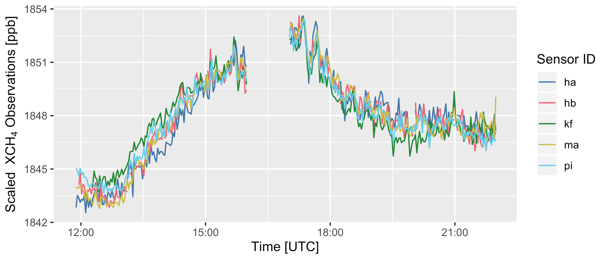
Figure 2 Total column dry mole fraction methane (XCH₄) for the five instruments on 1 of the 2 side-by-side intercomparison days. Calibration scaling factors have been applied to these data.

2.3 Aircraft and lidar observations

In addition to the total column measurements, four flights of Purdue University's Airborne Laboratory for Atmospheric Research (ALAR) aircraft were performed during the course of the campaign. These flights consisted of upwind and downwind transects of the city, as well as spirals in strategic locations. The ALAR was equipped with a Picarro model G2301-f cavity ring-down spectrometer (Crosson, 2008), which measured dry CO₂ and CH₄ concentrations in situ. High-frequency wind speed and direction data were also collected on the ALAR using the Best Air Turbulence (BAT) probe (Garman et al., 2006). Continuous wind measurements, as well as the height of the top planetary boundary layer (PBL), were monitored throughout the campaign using a wind Doppler lidar co-located with hb (Bonin et al., 2018). Although wind speeds and wind directions derived from the lidar data are less accurate than those from the aircraft, they still have utility in verifying the stability of the atmosphere and the accuracy of wind forecasts throughout the day. The ALAR wind data were used to compute daily wind error statistics, which were then used in the uncertainty calculations of our final results. ALAR and lidar data from throughout the campaign are shown in the Supplement.

2.4 Transport model

The Stochastic Time-Inverted Lagrangian Transport (STILT) model (Lin, 2003; Fasoli et al., 2018) was used to compute the sensitivity of the total column observations to surface emissions. The model simulates the movement of non-reactive trace gases by computing the trajectories of hypothetical massless particles released from the observation location and advected and diffused backwards in time according to a gridded meteorological product. For this work, the North American Mesoscale (NAM) 12 km product (Janjic and Gall, 2012) was used.

A linear model A can be created to relate emissions to our column observations.

$$\begin{array}{}\text{(1)}& \mathrm{\Delta }\mathit{y}=\mathbf{A}{\mathit{a}}_{\mathrm{s}}+{\mathit{\epsilon }}_a\end{array}$$

Here, the enhancement in the column due to emissions in the urban area is denoted Δy. The vector a_s consists of scaling factors for each sector. The matrix A contains the products of Lagrangian footprints, f, and a priori emissions fluxes, F. Error in the model due to uncertainties in the footprint values and observations is represented by the ε_a term.

The footprint as a function of location (x,y) and release time (t) can be expressed as

$$\begin{array}{}\text{(2)}& f(x,y,t)={\displaystyle \frac{m_{\mathrm{air}}}{h\left(t\right)\stackrel{\mathrm{‾}}{\mathit{\rho }}(x,y,t)}}{\displaystyle \frac{\mathrm{1}}{N_{\mathrm{p}}}}\sum _{i=\mathrm{1}}^{N_{\mathrm{p}}}\mathrm{\Delta }{t}_i(x,y),\end{array}$$

where m_air is the mean molar mass of air (29 g mol⁻¹), $\stackrel{\mathrm{‾}}{\mathit{\rho }}$ is the mean density of the air at coordinate ($x,y,t$), and N_p is the number of particles released. Δt_i is the amount of time particle i spent in coordinate (x,y), and h is the height of the mixing layer, which is typically defined as half the height of the PBL (Lin, 2003). The value of h is adjusted in the time steps immediately before the particle release to account for the time needed for these particles to vertically mix into the boundary layer (Fasoli et al., 2018).

In order to create slanted total column STILT footprints, model particles are released at altitudes of 25, 50, 75, 100, 150, 200, 300, 400, 600, 800, 1000, 1500, 2000, and 2500 m relative to the instrument location. These altitudes were chosen to be dense near the surface and more sparse nearer the top of the boundary layer. Particle releases at higher altitudes are not needed, as air significantly above the boundary layer does not interact with ground emissions on the scale of our domain.

Since the observed air mass is a slanted column with variable azimuth and solar elevation during the day (Hase et al., 2016), the latitude and longitude of the particle releases were adjusted based on the solar zenith and azimuth angles at the time of the release. We released 1000 particles from each level every 15 min. To create the total column footprint, f_c, footprints from the L=14 different altitudes are combined using a pressure weighting function, w(z). The weighting of the footprints can also be affected by the observing system's averaging kernel (A_k(z)), which is the relative sensitivity to concentrations at different altitudes. Since the averaging kernel of the EM27/SUN XCH₄ retrieval is ≈1 in the lower troposphere (Hedelius et al., 2016), this effect is minimal.

$$\begin{array}{}\text{(3)}& f_{\mathrm{c}}(x,y,t)=\sum _{i=\mathrm{1}}^{L}w\left(z_i\right)A_k\left(z_i\right)f_i(x,y,t)\end{array}$$

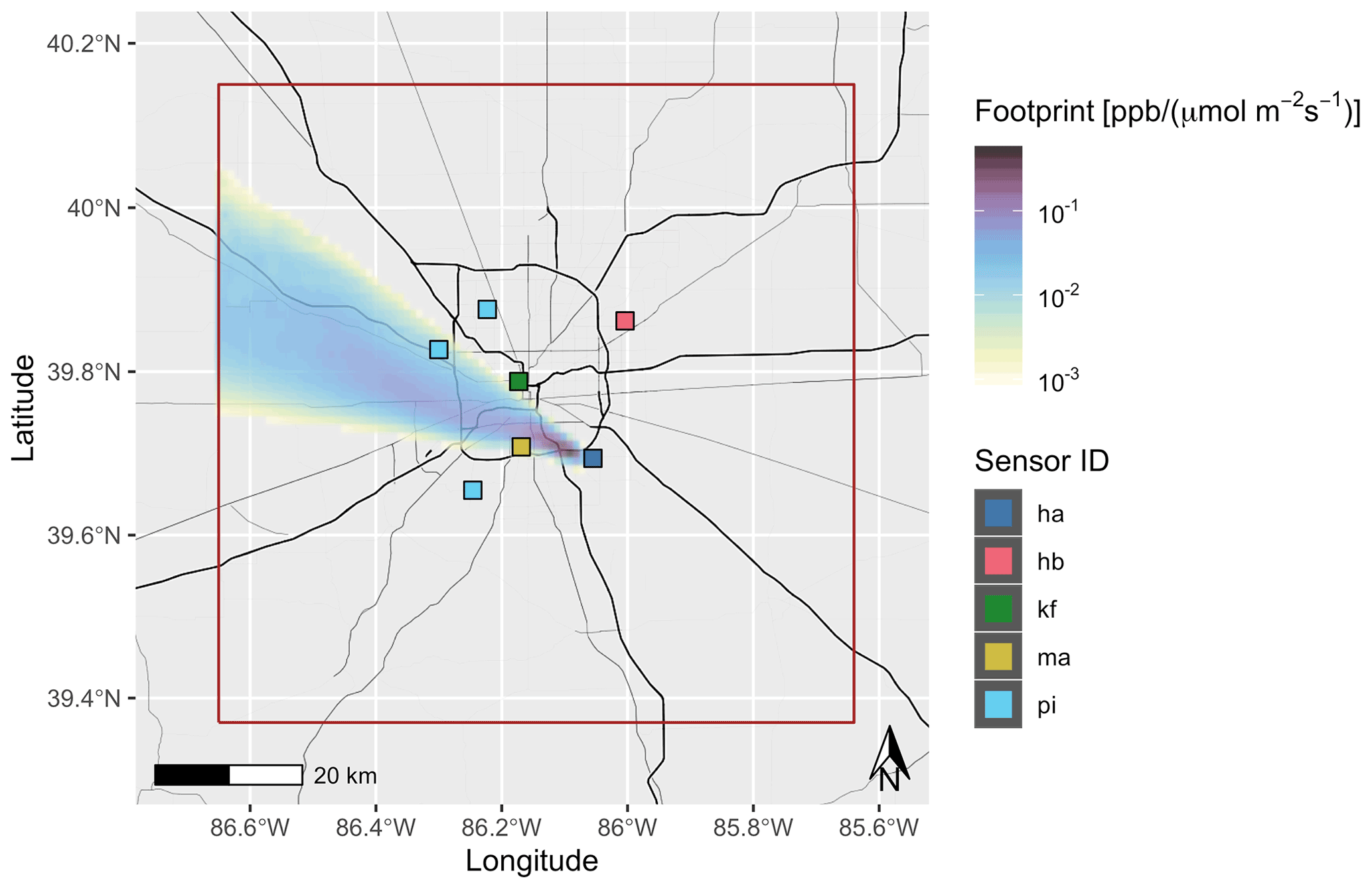
Figure 3 Total column footprint for sensor ha on 13 May 2016 at 12:30 UTC. The prevailing wind direction was from WNW, which resulted in ha being downwind of the city. Map tiles by Stamen Design under CC BY 3.0. Data by OpenStreetMap; © OpenStreetMap contributors 2020. Distributed under the Open Data Commons Open Database License (ODbL) v1.0.

This is similar to the “XSTILT” method for constructing STILT footprints for satellite observations (Wu et al., 2018). A more detailed description of this pressure weighting scheme is in the Supplement. An example total column footprint is shown in Fig. 3.

The column footprints are then multiplied by the a priori emissions field $F(x,y,s)$ and summed to produce a row n in the matrix A at the time step m. F is a function of latitude, x, longitude, y, and emissions sector, s, but is not temporally resolved. The resulting matrix A will have a number of columns equal to the number of observation time points being simulated and a number of rows equal to the number of emission sectors in the inventory.

$$\begin{array}{}\text{(4)}& {\mathbf{A}}_{m,n}=\sum _{i=\mathrm{1}}^{N_x}\sum _{j=\mathrm{1}}^{N_y}{f}_{\mathrm{c}}(x_i,y_j,t_m)F(x_i,y_j,s_n)\end{array}$$

Equation (4) represents the expected column-averaged methane enhancement at each measurement point in time due to urban methane emissions given an emissions field of dimension N_x×N_y. The values of A for the observations of 13 May are shown in Fig. 4. It is important to note that these prior expected enhancements are completely dependent on the prior emissions map and footprint values, and they are not influenced by any XCH₄ observations.

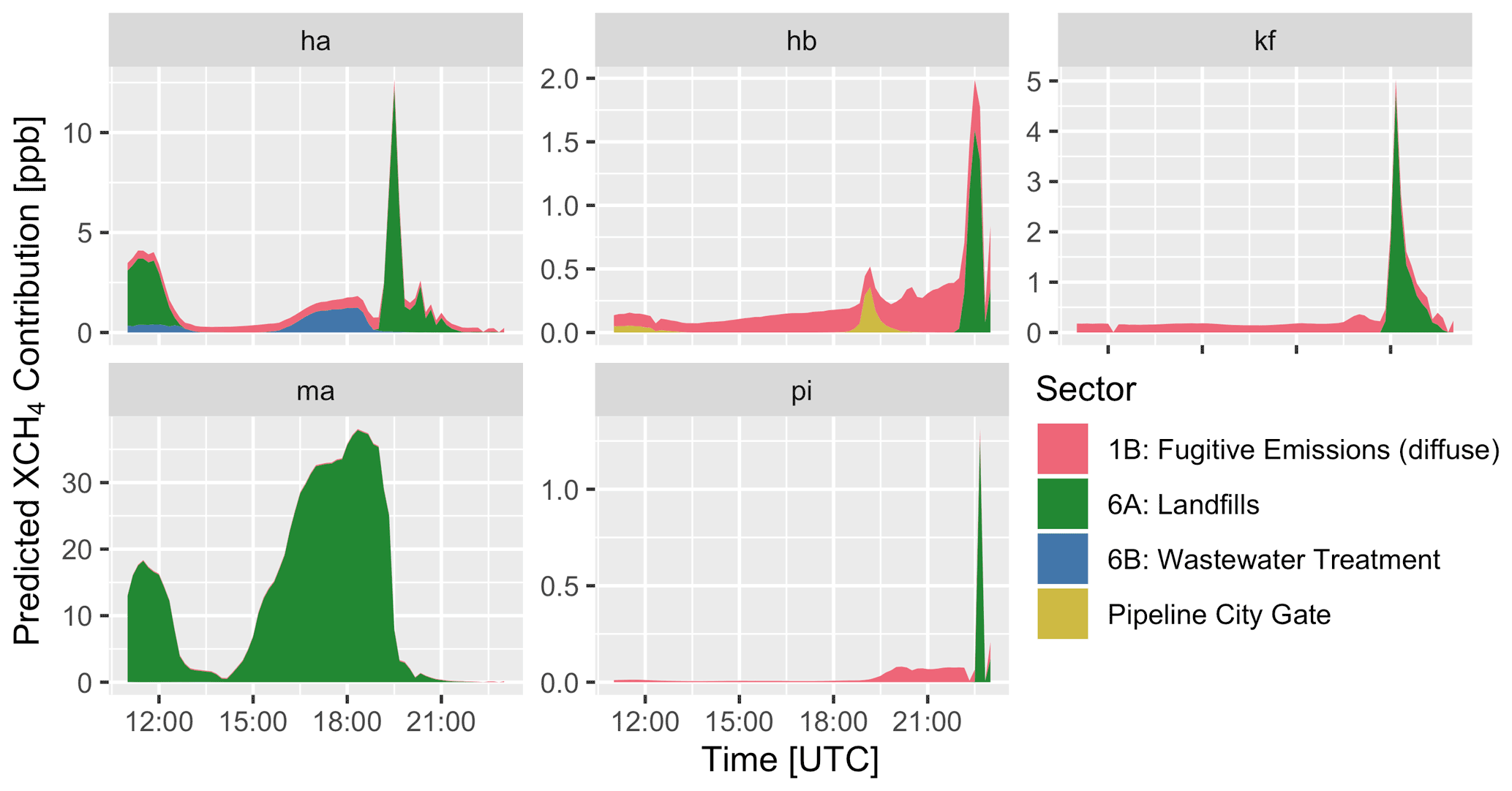
Figure 4 Predicted XCH₄ contribution to each measurement from each source for 13 May. These values are computed by multiplying the STILT footprints by the a priori inventory.

2.5 Background methane concentrations

Air entering the city has total column methane concentrations in excess of 1800 ppb, which can vary in time and space. The seasonal cycle is roughly ± 20 ppb, and latitude gradients across the Northern Hemisphere are roughly 50 ppb (Parker et al., 2011). Global mean XCH₄ is currently increasing at a rate of 7.6 (±0.4) ppb every year (Zhou et al., 2018), although the rate of increase of mean methane concentrations has not been consistent over the past few decades (Turner et al., 2019). As air moves over the continent, it can also entrain additional methane from emissions hundreds of kilometers upwind of the urban area of interest. The concentration of methane in the inflowing air (“background”) represents >99 % of the methane observed in the total column; therefore, variations in background concentrations during the experiment must be very accurately characterized.

Previous work that studied background methane concentrations in Indianapolis showed significant variations in the amount of methane in inflowing air and stressed the importance of carefully accounting for this effect (Balashov et al., 2020). Previous flux inversions of methane and other trace gases have dealt with the background in different ways. Many works have made an assumption that measurements from a sensor that is nominally upwind represent the inflowing air (McKain et al., 2015; Lamb et al., 2016; Chen et al., 2016; Sargent et al., 2018). In this work, however, a background time series is modeled using all of the network data. This additional step is required because of significant variations observed in the background over short timescales (<1 h). The background time series vector (b) represents the mean total column methane concentration along the domain boundary every 15 min, starting from the time when the first STILT particle enters the domain. The total column concentration is therefore modeled as the sum of the background entering the domain and the enhancement due to local emissions.

$$\begin{array}{}\text{(5)}& \mathit{y}=\mathbf{A}{\mathit{a}}_{\mathrm{s}}+\mathbf{B}\mathit{b}+{\mathit{\epsilon }}_{\mathrm{a}}+{\mathit{\epsilon }}_{\mathrm{b}}\end{array}$$

Here, B is the background influence matrix (BIM), which relates every observation to a distribution of influence from each background time point. Matrix B is unitless, as it merely transforms values from the boundary background (b, ppb) to background values at each observation point (also in parts per billion). An additional error term, ε_b, represents error (in ppb) in the background due to uncertainties in the BIM. It is important to note that because the values of the error terms ε_a and ε_b are unknown and can be quite large, a careful statistical inversion must be performed to retrieve valid estimates of emissions. The construction of B occurs during the computation of the STILT footprints. After defining the box that constitutes the edge of the domain, STILT particles are tracked backwards in time, and the time at which they cross the domain boundary is recorded. The relative influence of background air of different ages on observations at different sites is shown in Fig. 5, and the BIM of hb for the first measurement day (13 May) is shown in Fig. 6.

The particle releases used to create the BIM are the same as those used to create the footprints described earlier, so they are from 14 different altitudes up to 2500 m. Transport above this level is not modeled, which means there is a possibility that plumes present in the mid-troposphere will not be accounted for effectively.

Figure 5 Fraction of background influence for all sites on 13 May at 21:30 UTC. Although entries in the BIM are unitless, here they are shown divided by the background time step. These are therefore residence time probability density functions, with the integrals over the graphs each equal to 1.

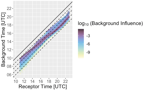
Figure 6 Background influence matrix (BIM) for instrument hb for the 13 May measurement day. The solid line is one-to-one and represents a residence time of 0 h within the modeling domain. The dashed lines represent residence times of 1, 2, 3, and 4 h within the modeling domain.

We can combine these linear operators into a single jacobian, K, which allows us to treat the entire measurement, emission, transport, and background model as a single linear system.

$$\begin{array}{}\text{(6)}& \mathbf{K}=\left[\mathbf{A}\mathbf{B}\right]\end{array}$$

The emissions scaling factors and domain background are then combined into a single state vector (x).

$$\begin{array}{}\text{(7)}& {\displaystyle }\mathit{x}=\left[\begin{array}{c}{\mathit{a}}_{\mathrm{s}}\\ \mathit{b}\end{array}\right]\text{(8)}& {\displaystyle }\mathit{y}=\mathbf{K}\mathit{x}\end{array}$$

2.6 Model uncertainty

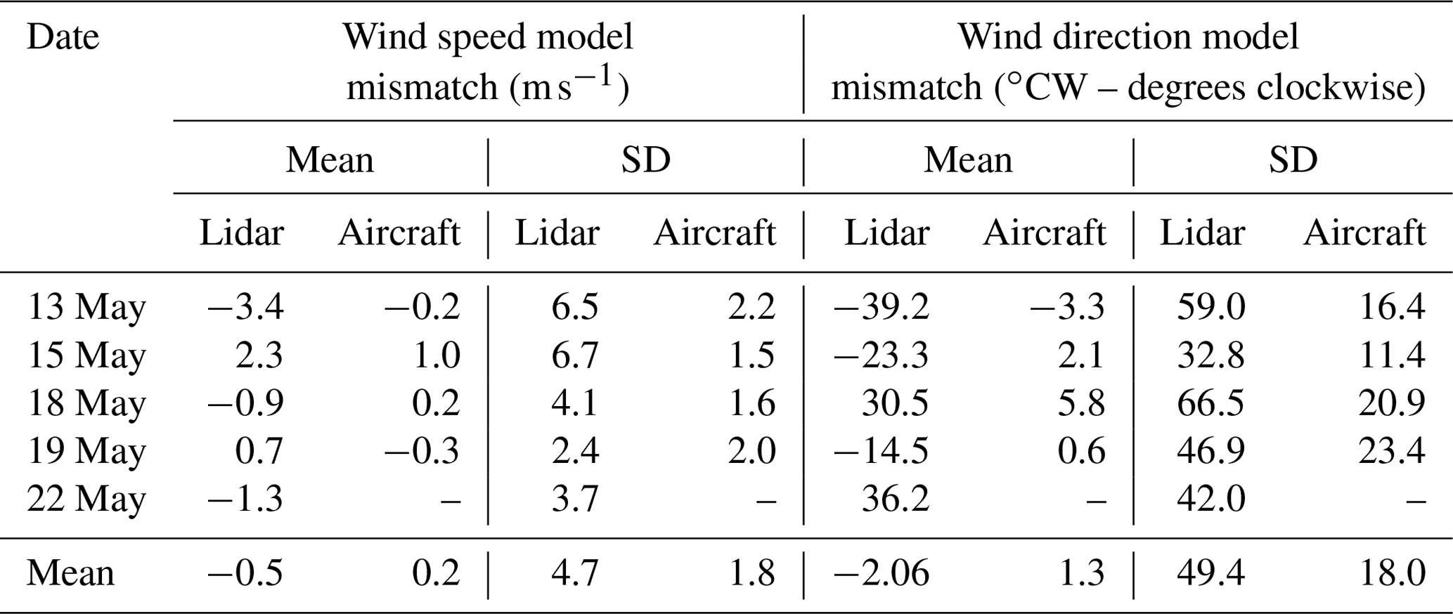
There are four main components to the uncertainty of the measurement–model system: background error (discussed previously), instrument measurement error, transport error, and source distribution error. The uncertainty of the EM27/SUN itself is taken from previous studies and assumed to be 0.2 ppb at 10 min integration times (Chen et al., 2016). The transport error is the uncertainty (in ppb) of a modeled total column observation due to uncertainties in the wind direction and wind speed used in the transport model. Using the ALAR observations, the relative wind errors could be computed. These calculations are shown in the Supplement. The results from the wind error analysis are shown in Table 3.

Table 3 Mean and standard deviations of wind speed and wind direction differences between the NAM model winds and observations from the ALAR aircraft and the wind lidar. Negative values indicate that the NAM model value is greater than the observation. The ALAR–NAM standard deviations for each day were used in the transport error analysis.

The method for determining the transport error associated with each observation is based on previous work addressing uncertainties in STILT (Lin and Gerbig, 2005; Fasoli et al., 2018); however, some major adjustments had to be made because of the nature of the domain in this study. A detailed description of this modified uncertainty calculation method can be found in the Supplement. The transport error analysis also allowed us to predict the likelihood that a given observation was influenced by any of the known point sources. If footprints with a point-source influence were not removed, it would be difficult to detect the diffuse source contribution. Methane enhancements due to concentrated emissions on the edge of a footprint are difficult to model accurately, so we developed a meticulous procedure to screen out footprints that could be influenced by our designated large point sources, as follows.

1. A STILT simulation (with 1000 particle releases at 14 altitudes) is performed.

2. Wind speed and direction statistics are established, and 500 transport error simulations are performed (see the Supplement).

3. Simulations in which at least 10 % of the expected methane enhancement are due to the known point sources (i.e., landfills, the wastewater treatment plant, or the city gate) are deemed to have a point-source contribution.

4. The likelihood of a point-source influence is then defined as the percentage of simulations that meet this criterion.

5. Observations that have a likelihood of point-source influence above a 50 % threshold are not included in the analysis of diffuse emissions.

The results of this threshold technique for the 5 d of the campaign are shown in Fig. 7. For example, more than 90 % of the observations from instrument ma were influenced by the nearby South Side Landfill on 3 d of the 5 d. The wind direction was different for the other 2 d: 18 and 19 May (see the Supplement). Some of the observations from site ha on 13 and 15 May also had to be discarded, as that sensor saw an occasional influence from both the landfill and the wastewater treatment plant.

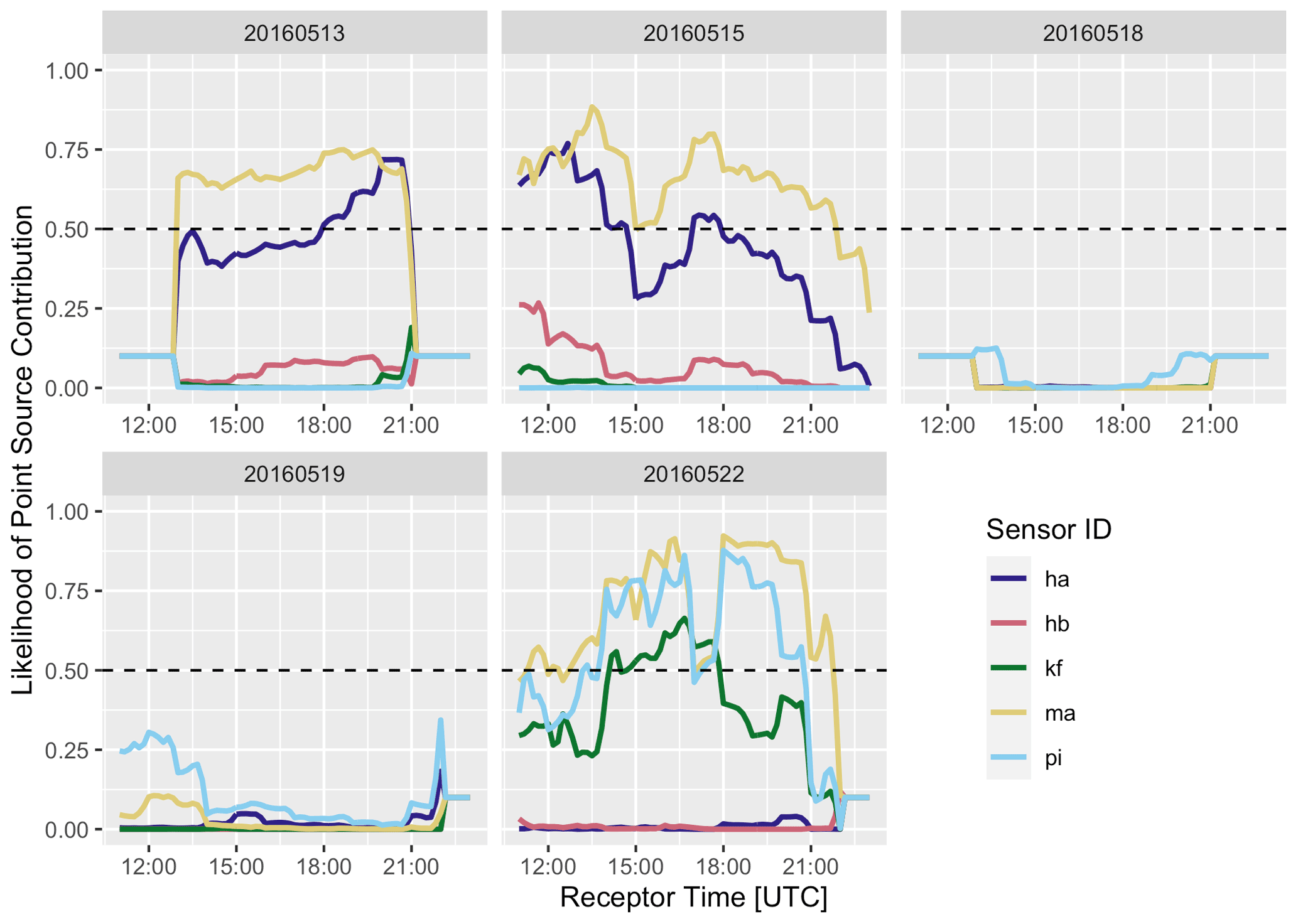
Figure 7 Likelihood of point-source contribution for each site throughout the campaign. The threshold level, 50 %, is shown by the dashed line.

The computed uncertainties in the total column methane concentration due to horizontal transport error are shown in Fig. 8. Locations upwind of the city, such as pi on 13 and 15 May, have a much lower value than downwind sites even though they experience the same amount of wind error. This is because the emissions upwind of pi (but still inside the domain) on these days are both weak and spread out, which means that shifts in the wind direction do not greatly affect the amount of methane observed at this location. This analysis gives us the ability to weight observations differently based on this error when computing the mean rate of urban emissions.

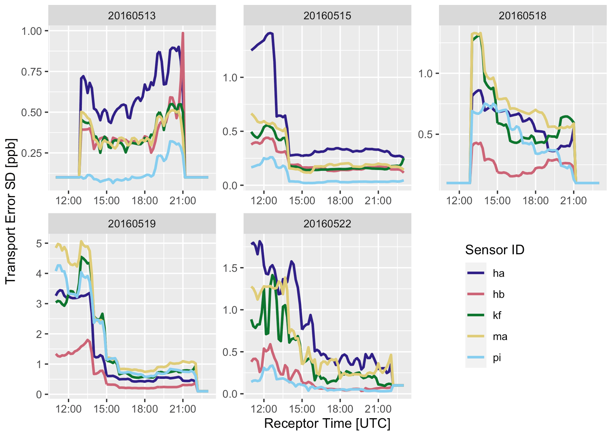
Figure 8 Standard deviations due to uncertainties in horizontal transport for the entire campaign.

2.7 Uncertainties in diffuse emission distribution

Diffuse emissions were assumed to be distributed around the urban area using a method based on the high-resolution HESTIA database. To test the sensitivity of the inversion to this distribution, two other distributions were also examined, as shown in Fig. 9. The first partitions emissions based on population density, which can be assumed to be a proxy for the density of residential natural gas usage. If incomplete combustion and leakage are issues in household gas appliances, such as stoves and water–air heating systems, this could be a reasonable prior distribution of diffuse emissions. The second partitions emissions based on road density. Since urban natural gas pipes run underneath and along roads, this could be a reasonable prior for the distribution of leaks in pipes (Phillips et al., 2013). Both of these new inventories were scaled so that the total emissions from all three methods were equal.

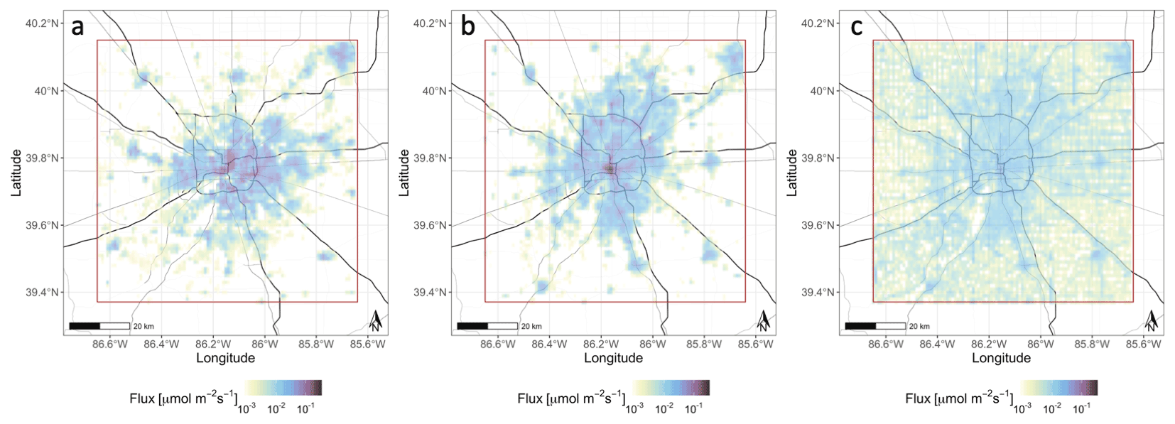
Figure 9 Diffuse emission spatial distributions based on (a) HESTIA, (b) population, and (c) road density. Map tiles by Stamen Design under CC BY 3.0. Data by OpenStreetMap; © OpenStreetMap contributors 2020. Distributed under the Open Data Commons Open Database License (ODbL) v1.0.

2.8 Bayesian framework

Uncertainties associated with the measurements, the prior estimate, and the transport model are all accounted for by using a linear Bayesian inversion framework (Rodgers, 2000). This method focuses on the reduction of a cost function, 𝒥(x), which weights the discrepancies between the model, observations, and prior estimates based on their uncertainties. If these uncertainties are assumed to be normally distributed, the log-likelihood cost function can be expressed as follows (Turner et al., 2018).

$$\begin{array}{}\text{(9)}& \begin{array}{rl}\mathcal{J}\left(\mathit{x}\right)& ={\displaystyle \frac{\mathrm{1}}{\mathrm{2}}}(\mathbf{K}\mathit{x}-\mathit{y}{)}^T{S}_{\mathit{\epsilon }}^{-\mathrm{1}}(\mathbf{K}\mathit{x}-\mathit{y})\\ & +{\displaystyle \frac{\mathrm{1}}{\mathrm{2}}}({\mathit{x}}_{\mathrm{a}}-\mathit{x}{)}^{\mathrm{T}}{S}_{\mathrm{a}}^{-\mathrm{1}}({\mathit{x}}_{\mathrm{a}}-\mathit{x})\end{array}\end{array}$$

The prior state vector (x_a) contains initial estimates of the scaling factors for the emissions from each sector, as well as initial estimates of the background methane concentration at every relevant point in time. The entries corresponding to emissions scaling factors are all equal to 1, as the magnitude of the emissions map is the best a priori estimate of emissions. A background value of 1.84 ppm was chosen after a cursory look at the data. These values are not critical, as the framework assumes uninformed priors for all of the scaling factors and background values.

$$\begin{array}{}\text{(10)}& {\mathit{x}}_{{\mathrm{a}}_i}=\left\{\begin{array}{ll}\mathrm{1},& \mathrm{1}\le i\le n_{\sec }\\ & \text{prior estimates of scaling factors}\\ \mathrm{1.84},& \mathrm{otherwise}\\ & \text{prior estimates of boundary}\\ & \text{background in ppm}\end{array}\right.\end{array}$$

Here, n_sec is the number of sectors. The first diagonal elements of the prior covariance structure S_a are the variances of the scaling factors of the emission sectors ${\mathit{\sigma }}_{\mathrm{s}}^{\mathrm{2}}$ and are chosen to be large (≫1). Having a weakly informative prior allows the inversion to produce emission values that are dependent on the observations, while still relying on the spatial distribution established by the prior. The remaining diagonal elements are the estimated uncertainties in the background estimate. These values are also chosen to be large, as the magnitude of the background signal is not known a priori.

$$\begin{array}{}\text{(11)}& {\mathbf{S}}_{{\mathrm{a}}_{i,j}}=\left\{\begin{array}{ll}{\mathit{\sigma }}_{\mathrm{s}}^{\mathrm{2}},& i,j\le n_{\sec }\mathrm{and}i=j\\ & \text{Variance of prior scaling}\\ & \text{factor estimates}\\ \mathrm{0},& i,j\le n_{\sec }\mathrm{and}i\ne j\\ & \text{Assumed zero covariance}\\ & \text{between sectors}\\ {\mathit{\sigma }}_{\mathrm{b}}^{\mathrm{2}}{e}^{-\left|\mathrm{\Delta }{t}_{i,j}\right|/T_{\mathrm{b}}},& i,j>n_{\sec }\\ & \text{Background values covary}\\ & \text{with dependence of time}\\ & \text{between points}\end{array}\right.\end{array}$$

In Eq. (11), the amount of time, in hours, between observations i and j is represented by Δt_i,j. Most of the off-diagonal elements represent the correlation in errors between background concentrations, which is a function of how smoothly the background is expected to change. A background covariance timescale (T_b) of 3 h was used. This value was chosen so that synoptic and mesoscale wind patterns (Van Der Hoven, 1957) would be accounted for. Higher-frequency (i.e., eddy-scale) variations in wind speed are not accounted for in the NAM model, so a shorter background covariance timescale could not be used.

The model–observation covariance structure S_ε represents the total uncertainties of the transport model and the observations. The values of S_ε are dependent on factors such as uncertainties in the wind and heterogeneity of the prior emissions field. A modified version of the framework first described in Lin and Gerbig (2005) is used to compute the values for each observation. This framework requires estimations of standard deviations of wind speed, wind direction, and PBL height errors of the meteorology model, as well as correlation length scales and timescales for these errors. The length scales for these types of errors are typically larger (>1 km) than the domain of interest in this study, so it is a reasonable assumption that the wind errors are completely correlated. The variance of the wind speed and wind direction errors was derived from the aircraft spiral observations as discussed in the Supplement.

There is an analytical solution for the cost function 𝒥(x), which is the maximum a posteriori (MAP) solution for the background time series and diffuse emissions scaling factor,

$$\begin{array}{}\text{(12)}& \widehat{\mathit{x}}={\mathit{x}}_{\mathrm{a}}+\mathbf{G}(\mathit{y}-\mathbf{K}{\mathit{x}}_{\mathrm{a}}),\end{array}$$

where G is the gain matrix:

$$\begin{array}{}\text{(13)}& \mathbf{G}={\mathbf{S}}_{\mathrm{a}}{\mathbf{K}}^{\mathrm{T}}({\mathbf{KS}}_{\mathrm{a}}{\mathbf{K}}^{\mathrm{T}}+{\mathbf{S}}_{\mathit{\epsilon }}{)}^{-\mathrm{1}}.\end{array}$$

The uncertainties of the values of $\widehat{\mathit{x}}$ are computed by the construction of a posterior covariance matrix, S_p, the diagonals of which describe the model framework's ability to reduce the uncertainties of the priors (Rodgers, 2000). It should be noted that this posterior will likely be dependent on the prior uncertainties chosen and that a rigorous inversion should have reasonable prior estimates of error.

$$\begin{array}{}\text{(14)}& {\mathbf{S}}_{\mathrm{p}}=({\mathbf{K}}^{\mathrm{T}}{\mathbf{S}}_{\mathit{\epsilon }}^{-\mathrm{1}}\mathbf{K}+{\mathbf{S}}_{\mathrm{a}}^{-\mathrm{1}}{)}^{-\mathrm{1}}\end{array}$$

This formulation, like the above formula for $\widehat{\mathit{x}}$, assumes that the prior has a Gaussian distribution (Turner et al., 2018).

3 Results

3.1 EM27/SUN observations

Measured XCH₄ values (Fig. 10) showed large variations throughout the day that are in excess of 10 ppb on some of the days. Some of these variations propagate across the city from upwind to downwind locations, suggesting that these result from spatial and temporal variations present in the inflowing air and not due to emissions within the city. The gradients between sites were much smaller: on the order of 1 ppb across the city. The influence of the South Side Landfill, particularly on instrument ma, was evident in the form of high-frequency variations of 10–20 ppb. As noted above, the observations affected by landfill emissions were screened out of the inversion using the STILT footprints.

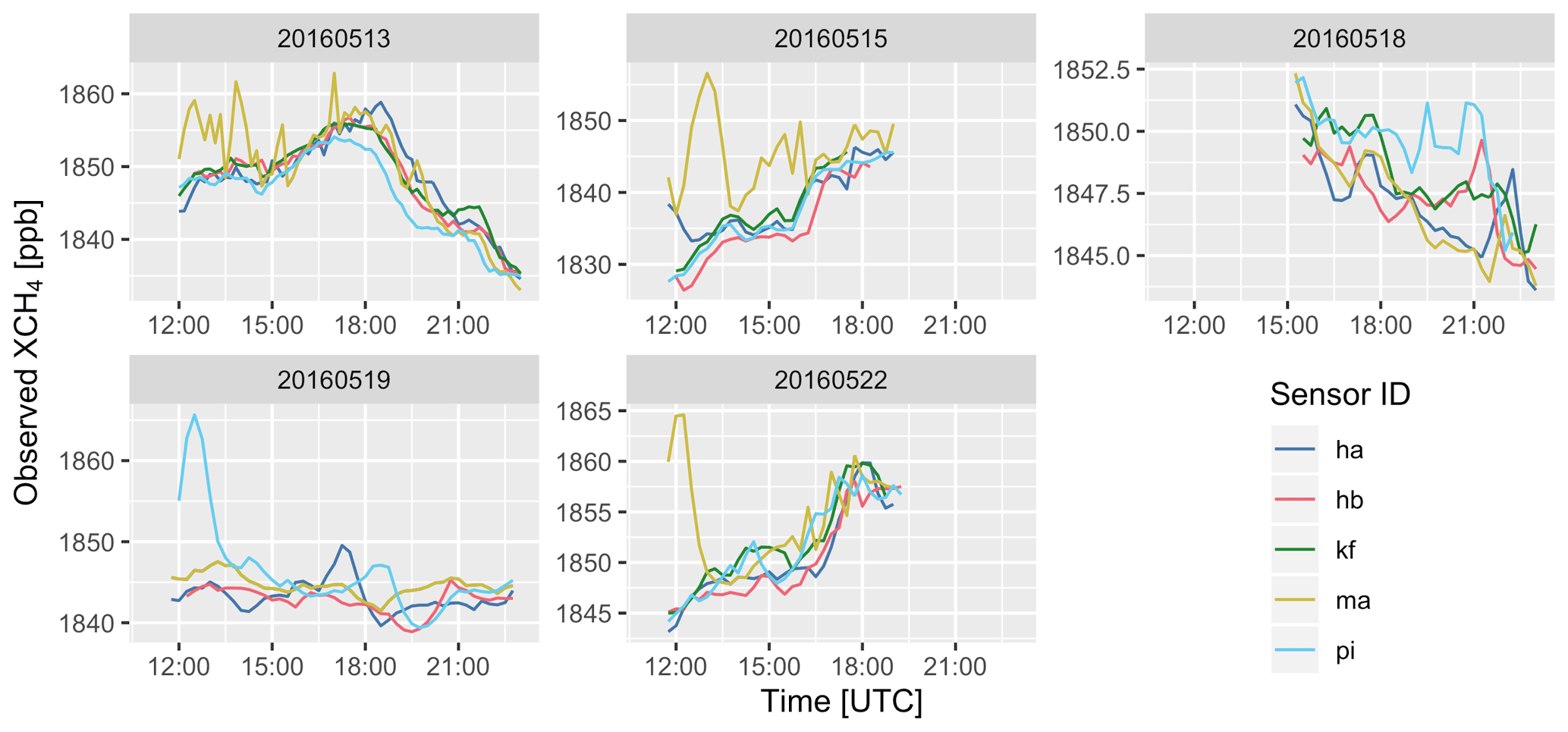
Figure 10 Total column dry mole fraction methane (XCH₄) for the five sensors on all 5 d of the campaign. The high-frequency signal for sensor ma is due to its close proximity to the South Side Landfill, the largest point source in the city.

3.2 Inversion results

The diffuse emissions scaling factors are summarized in Table 4. The model scaled the diffuse emissions from a prior value of 43.4 mol s⁻¹ to a value of 73.3 (±22) mol s⁻¹ with 95 % confidence. The daily Bayesian inversions were able to adequately model background concentration time series that captured the dynamics of the plumes observed, including on 13 May when the background variation was the highest of all measurement days (Fig. 11). The model was also able to fit the EM27/SUN observations very well (Fig. 12). However, since most of the variation in XCH₄ was due to variation in the background, this fit does not represent the ability of the model to constrain emissions. The observed and modeled enhancements (Fig. 13) give a clearer view of the emissions signal, which is small but clearly observable. In order to test the significance of the correlation between observed and modeled enhancements, points were binned into 0.5 ppb wide bins based on model enhancement values. The mean observed enhancement values for the 0–0.5 and 1–1.5 ppb bins were then tested to see if the were significantly distinct, resulting in a p value of 0.003. This result suggests that even with such a small signal level and in the presence of large background concentration variations, the model was able to detect and quantify enhancements in methane due to urban emissions.

Table 4 Inversion results for the diffuse sector for all 5 d of the campaign; 95 % confidence intervals are computed using the posterior error variances.

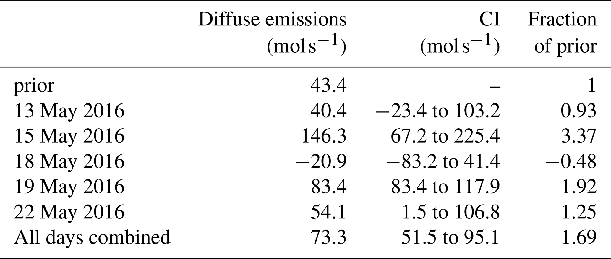
Although we are confident that the model framework was able to detect meaningful methane fluxes using all 5 d of data, the daily inversions yield emission numbers that vary greatly and are sometimes nonphysical, such as the negative emissions reported on 18 May. This shows that a single day of measurements is unlikely to produce a robust result; even the combination of all 5 d should be viewed as an experimental proof of concept, and continuous measurements for many months should be used to produce a more compelling final emission number.

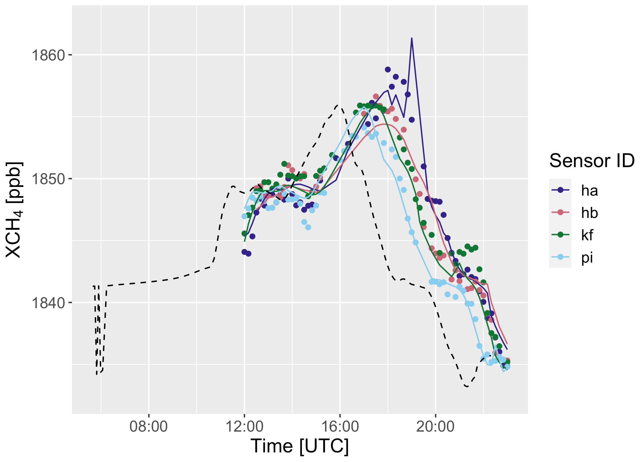
Figure 11 Observed XCH₄ values for 13 May (shown in points). Optimized domain boundary background values (gray, dashed) and optimized total column values, including urban emissions (colored lines), are also shown.

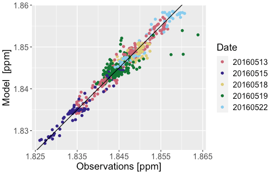
Figure 12 Optimized model correlation with the 5 d observations. The black curve is a 1–1 line. Each point represents a 15 min average from a single sensor. Observations with a significant point-source influence have been removed.

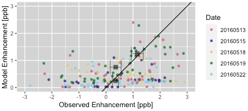
Figure 13 Optimized model correlation with the observations. The modeled background influence has been subtracted from both, showing just the enhancement in the total column due to local diffuse sources. The black line is a 1–1 line. These points represent 1 h averages. Gray squares represent the mean observation values when model values are divided into 0.5 ppb wide bins. The horizontal error bars represent the sample standard deviations for each bin. The means of the first (0.0–0.5 ppb) and third (1.0–1.5 ppb) bins are significantly distinct (p=0.003), demonstrating detection and quantification of the small enhancements in total column methane attributable specifically to diffuse emissions.

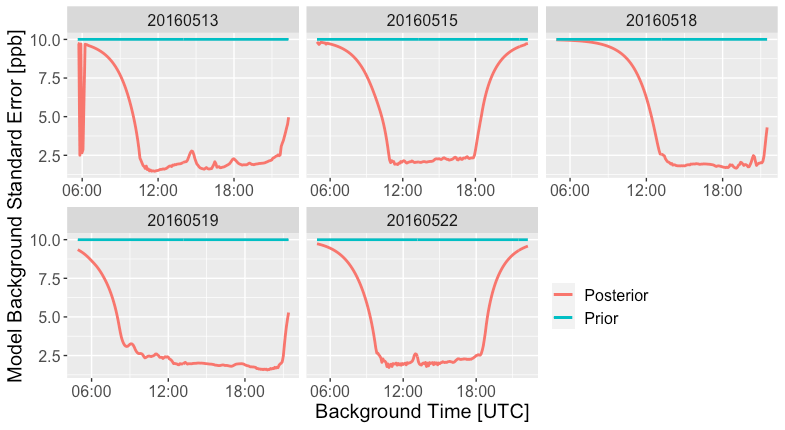
The background error, which was given an arbitrary large prior value of σ_bk=10 ppb, was reduced to less than 1 ppb in the posterior for background times in the middle of the day (see Fig. 14). This shows that the model was able to constrain this additional parameter in a meaningful way. Background values at the start and end of the day are less constrained, as their relative influence on the observations is smaller.

Figure 14 Posterior values for modeled background standard error.

The effect of using different flux spatial distributions is shown in Fig. 15. Using a distribution based on road density resulted in diffuse emissions being scaled up by more than 500 %, up to 301.4 (±70) mol s⁻¹. This is because the road-based distribution shifted a large portion of emissions to roadways outside the city center, lowering the prior emissions in the downtown area. The population-based distribution, while more similar to the HESTIA product, also shifted some of the emissions from downtown. The inversion using the population-based distribution increased diffuse emissions to 117.9 (±28) mol s⁻¹, which is higher than the HESTIA-based inversion (73.3 mol s⁻¹) and the prior (43.4 mol s⁻¹).

Figure 15 Total diffuse emissions from inversions using three different spatial distributions. The prior estimate of 43 mol s⁻¹ is shown with a dashed line.

The results of this analysis are compared with other published results and bottom-up inventories in Fig. 16. Not all of the inventories categorize emissions the same way, so the closest IPCC sector for each category was chosen for each inventory sector. Since this study is focused on diffuse emissions, the contributions from non-diffuse sources are taken directly from the prior.

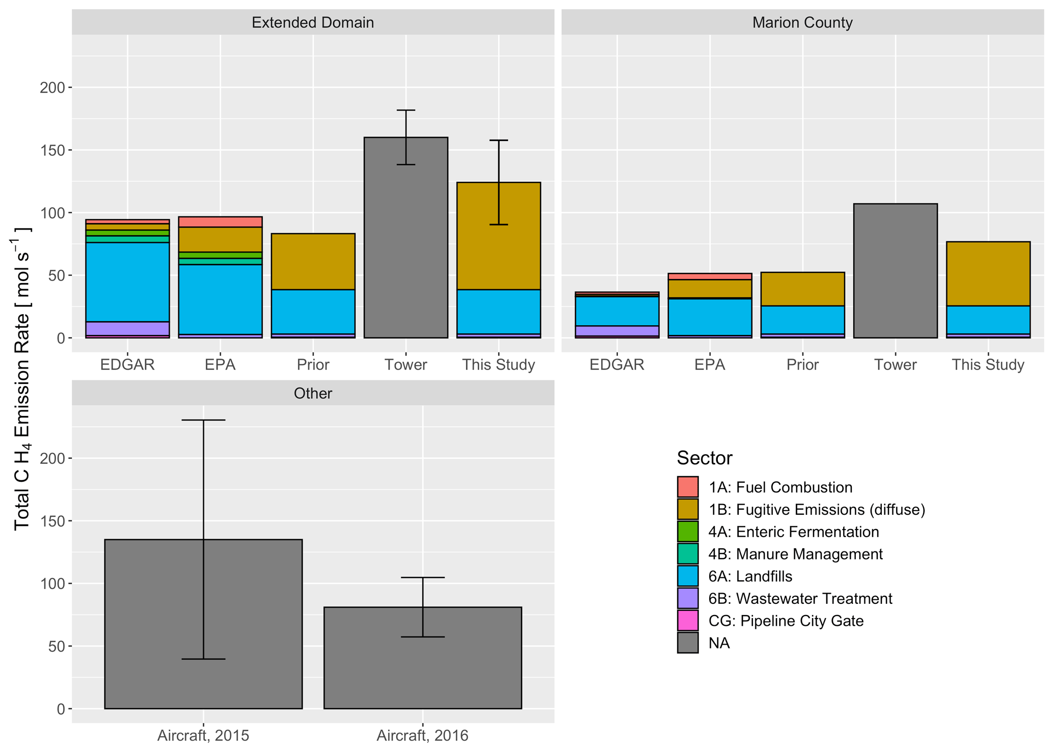
Figure 16 Comparison of total methane emission estimates for the domain. The EPA inventory (0.01^∘ resolution) (Maasakkers et al., 2016), and the EDGAR version 4.3 database (0.1^∘ resolution) (European Commission, 2011) were interpolated to the domain. The emission prior and tower inversion results are from a previous study (Lamb et al., 2016). These inventories were separated by IPCC emission sectors (IPCC, 2006). Emissions from a smaller subset of the domain (Marion County) were also computed by scaling the emissions in that area by the posterior scaling factor. Emissions computed by using aircraft mass balance techniques (Cambaliza et al., 2015), which do not necessarily conform to either spatial domain, are also shown for comparison. Error bars for the tower and aircraft studies represent the reported 95 % confidence intervals from their results. The error bars shown for this study represent the 95 % confidence interval based on the posterior error variances.

4 Conclusions

We created a network of EM27/SUN spectrometers to enable distributed, efficient sampling of total column methane at high spatial resolution from the ground in and around the city of Indianapolis. Enhanced methane concentrations due to diffuse emissions from the urban core, likely from leaks and inefficiencies in the natural gas distribution system, were detected and quantified as distinct from methane originating from large identified point sources. Our observations suggest that the magnitude of diffuse emissions in notably larger than the values presented in bottom-up inventories. Our results are consistent with the independent analysis of data from tower-based sensors as shown in Fig. 16. Although our measurement and data analysis techniques are newer and not as established as the other method shown in Fig. 16, we believe that our result supports the findings shown in these other studies. Since all of these methods have different drawbacks and make different sets of assumptions, any attempt to truly quantify emissions from such a complex source should consider as many independent methods as possible.

Variations in the inversions results (Fig. 15) between each day are quite large, but this is not surprising. Different days have significantly different wind patterns, which means different sections of the city are sampled on different days. If the inventory needs to be adjusted by different amounts for different sections of the domain, which is likely, the model will compute different scaling factors. By ingesting large amounts of data over a long time frame covering many wind patterns, this issue can be resolved. Ideally, significantly more data than the 5 d used in this experimental study would be used.

Another improvement would be to solve for different scaling factors in different parts of the city. Theoretically, the inversion can solve for each grid square independently, with correlations between squares expressed in the covariance matrices. However, in practice this requires significantly more observations because the results become less constrained as the state vector increases in length. We believe that our framework could easily be expanded to spatially resolve emissions if implemented with data from a permanent or semipermanent installation of sensors, such as MUCCNET (Dietrich et al., 2021).

Although this study uses only a few days of data, our results confirm the significance of diffuse methane emissions in urban areas. Even though the city of Indianapolis has relatively modern natural gas delivery systems, fugitive emissions represent more than half of all methane released into the atmosphere. This information is critical for those tasked with mitigating emissions and suggests that increased investment in leak detection and repair efforts would make a measurable impact on the overall emission rate of a city. In order to assess the magnitude of diffuse methane emissions and to measure the effect of mitigation efforts, more cities need to implement measurement networks like the one developed here and maintain them for long periods.

This work also highlights several factors that need to be carefully considered when designing a ground-based measurement network and accompanying model framework. For instance, an analysis of dominant wind conditions should be performed and sensor locations should be chosen so that there is minimal likelihood that sensors will observe intermittent point-source influence. Alternatively, if the objective of the network is to quantify a point source, that likelihood should be maximized, as intermittent influence would make that quantification more difficult. Furthermore, having portable sensors, like the EM27/SUN, allows different locations to be chosen on a daily basis to improve the quality of the measurement if siting logistics are predetermined.

The characteristics of the inflowing (i.e., background) air are also of great importance, as hourly variations in background concentrations can be larger than the signal from the city itself. We present a novel inversion framework that accounts for the temporal variation of the background and determines the influence of the background concentrations at the measurement points. We assume constant concentrations along the edge of the domain, which is reasonable in a city like Indianapolis but would not be practical in other locations with complicated terrain, heterogeneous wind patterns, and strong upwind point sources. When designing a network and model framework, a background quantification technique that fits the specific conditions of the area of study should be chosen.

The spatial distribution of diffuse sources must also be carefully considered, as this can have large impacts on the inversion results, as shown in Fig. 15. Although all three spatial distributions tested in this study suggest more emissions than present in the bottom-up inventory, the magnitudes differ significantly depending on how much weight is given to the core of the city. Distributing emissions based on road density resulted in a much larger posterior estimate than the other two methods because the road-based distribution shifts emissions from the center of the city to the suburbs, which are under-sampled by the network. The inversion using the population-based distribution also suggests somewhat larger emissions than the HESTIA-based distribution because the population distribution does not account for emissions from commercial and industrial facilities concentrated in the core of the city. It is important to note that the inversion framework described here does not have a mechanism for incorporating spatial uncertainty and cannot redistribute emissions around the domain. Testing multiple plausible distributions gives a sense of the sensitivity of the model, and we suggest that any comprehensive analysis include model inversions using several distributions.

When an inversion is performed using the road-based distribution and all of the days of data, the estimate of emissions is much higher than any of the individual days. This is because the road-based distribution pulls emissions from the center of the city and puts them in the outer ring roads, which have a significantly lower total footprint. This means that the product of the footprints and emissions grid is relatively low, and therefore the model gives more weight to the prior. Only when all of the days are used are there enough data to influence the model significantly. Because the road-based distribution has relatively low prior emissions in the city center, the result is a large scaling factor. This also highlights the importance of sensor placement. Sensors should be placed close to the bulk of the suspected emissions sources so that strong influence is detected in a variety of wind conditions. If the experiment was designed with the road-based distribution in mind, sensors would be placed further apart in order to adequately sample the ring roads. We also suggest that more sensors would be needed in this situation, as a greater portion of emissions would be spaced out over a larger area.

The size and shape of the domain must also be carefully chosen, as this will affect the ability of the model to correctly characterize inflowing air. The choice of domain can also affect the ability to compare the results to those of other studies, as shown in Fig. 16, and consideration should be given to policy-relevant domains, such as city limits and county and state boundaries.

Future studies utilizing these types of instruments should also explore the trade-offs involved when choosing the number of sensors needed and their placement. While some studies exploring this concept have been performed using similar footprint methods, they have mostly been done for in situ sensor networks (Turner et al., 2018; Lopez-Coto et al., 2020, and total column sensors require a different set of considerations. For instance, the footprints of total column sensors are larger, which means fewer sensors are needed to sample the same area. Also, although portable FTIR systems may not be cheaper than many in situ sensors, they do not require the presence of tall buildings or investment in tower infrastructure in order to be deployed, which makes finding suitable deployment sites easier. Data collection with total column systems is also dependent on direct sunlight, so any study exploring the utility of these types of networks in a specific region should also consider weather, solar angles, and shading.

As higher-resolution satellites are developed to measure greenhouse gas emissions from complex sources, it is important to understand the magnitude and variation of total column concentrations on these scales. This work shows that in order to detect methane emissions from a source like the city of Indianapolis, an observing system must be able to accurately measure concentration gradients of less than 1 ppb in the total column. Furthermore, any such system must also have a method for discerning the influence of background methane concentrations. Although satellite observations will benefit from having spatially dense observations, sensors in low-Earth orbit are not likely to have good temporal resolution. This makes the identification of passing plumes even more difficult. Sensors like the EM27/SUN will likely provide complementary information and play an increasing role in the development, validation, and calibration of aircraft and satellite trace gas remote sensing missions. Conventional validations, such as comparisons to the few TCCON stations scattered throughout the globe, will be insufficient as these new sensors attempt to quantify small signals in complex situations. Although there are certainly trade-offs compared to tower-based in situ sensors (such as being limited to clear-sky daylight hours), portable ground-based total column measurement systems have shown their usefulness as a component to a robust urban methane measurement network. As more and more cities seek to quantify their carbon emissions at policy-relevant scales, it will be essential to employ innovative transport models and a diverse set of instruments, including ground-based total column sensors.