Statistical properties of a stochastic model of eddy hopping

Statistical properties are investigated for the stochastic model of eddy hopping, which is a novel cloud microphysical model that accounts for the effect of the supersaturation fluctuation at unresolved scales on the growth of cloud droplets and on spectral broadening. Two versions of the model, the original version by Grabowski and Abade (2017) and the second version by Abade et al. (2018), are considered and validated against the reference data taken from direct numerical simulations and large-eddy simulations (LESs). It is shown that the original version fails to reproduce a proper scaling for a certain range of parameters, resulting in a deviation of the model prediction from the reference data, while the second version successfully reproduces the proper scaling. In addition, a possible simplification of the model is discussed, which reduces the number of model variables while keeping the statistical properties almost unchanged in the typical parameter range for the model implementation in the LES Lagrangian cloud model.

1 Introduction

The purpose of the present paper is to investigate the statistical properties of the stochastic model of eddy hopping proposed by Grabowski and Abade (2017). This stochastic model, referred to hereinafter as the eddy-hopping model, was developed in order to account for the effect of the supersaturation fluctuation at unresolved (subgrid) scales on the growth of cloud droplets by the condensation process. In a turbulent cloud, cloud droplets arriving at a given location follow different trajectories and thus experience different growth histories, which leads to significant spectral broadening. This mechanism, referred to as the stochastic condensation theory, has been investigated since the early 1960s by a number of researchers (mostly Russian; see Sedunov, 1974; Clark and Hall, 1979; Korolev and Mazin, 2003), but the importance of this mechanism was later reinforced by Cooper (1989) and Lasher-Trapp et al. (2005). For this mechanism, Grabowski and Wang (2013) emphasized the importance of large-scale eddies (turbulent eddies with scales not much smaller than the cloud itself) and proposed the concept of large-eddy hopping. Grabowski and Abade (2017) formulated this concept and developed the eddy-hopping model. Abade et al. (2018) extended the model by introducing a term accounting for the relaxation of supersaturation fluctuations due to turbulent mixing. For clarity, we hereinafter refer to the model by Grabowski and Abade (2017) as the original version, and the model by Abade et al. (2018) as the second version. For the following study using the eddy-hopping model, readers are referred to Thomas et al. (2020).

It should be noted that the turbulent entrainment mixing is another important mechanism for the supersaturation fluctuation generation other than the stochastic condensation and that the effects of the turbulent entrainment mixing are not included in the eddy-hopping model considered in the present study. Abade et al. (2018) investigated the effects of the turbulent entrainment mixing and entrained CCN activation by using the entraining parcel model.

In the present paper, we take a rather theoretical approach to obtain various statistical properties of the eddy-hopping model, such as the variance, covariance, and auto-correlation function of the supersaturation fluctuation. These statistical properties are used to validate the model against the reference data taken from direct numerical simulations (DNSs) and large-eddy simulations (LESs). We show that the original version of the eddy-hopping model fails to reproduce a proper scaling for a certain range of parameters, resulting in the deviation of the model prediction from the reference data, while the second version successfully reproduces the proper scaling. We show how the relaxation term introduced by Abade et al. (2018) leads to this improvement. We also discuss the possibility of simplification of the model, which reduces the number of model variables while keeping the statistical properties almost unchanged in the typical parameter range for the model implementation in the LES Lagrangian cloud model.

The remainder of the present paper is organized as follows. Section 2 describes the governing equations of the original version. Section 3 presents a theoretical analysis and numerical experiments and demonstrates the improper scaling in the model prediction by the original version. Section 4 describes the second version. Finally, Sect. 5 discusses the possibility of simplification of the model.

2 Governing equations

The original version of the eddy-hopping model proposed by Grabowski and Abade (2017) consists of the following two evolution equations. First, the fluctuation of the vertical velocity of turbulent flow at the droplet position, w^′(t), is modeled by the Ornstein–Uhlenbeck process:

$$\begin{array}{}\text{(1)}& {\displaystyle }{w}^{\prime }(t+\mathit{\delta }t)=w^{\prime }\left(t\right){\mathrm{e}}^{-\mathit{\delta }t/\mathit{\tau }}+\sqrt{\mathrm{1}-{\mathrm{e}}^{-\frac{\mathrm{2}\mathit{\delta }t}{\mathit{\tau }}}}{\mathit{\sigma }}_{w^{\prime }}\mathit{\psi },\end{array}$$

where δt is the time increment, ψ is a Gaussian random number with zero mean and unit variance drawn every time step, ${\mathit{\sigma }}_{w^{\prime }}$ is the standard deviation of w^′, and τ is the integral time, or the large-eddy turnover time of the turbulent flow. Here, ${\mathit{\sigma }}_{w^{\prime }}$ and τ are used as the model parameters. Second, the supersaturation fluctuation at the droplet position, S^′(t), is governed by

$$\begin{array}{}\text{(2)}& {\displaystyle \frac{\mathrm{d}{S}^{\prime }}{\mathrm{d}t}}=a_{\mathrm{1}}{w}^{\prime }-{\displaystyle \frac{S^{\prime }}{{\mathit{\tau }}_{\mathrm{relax}}}}.\end{array}$$

Here, the first term on the right-hand side represents the effect of adiabatic cooling and warming due to air parcel ascent and descent caused by the vertical velocity w^′(t). The parameter a₁ has the unit of a scalar gradient. The second term on the right-hand side represents the effect of condensation or evaporation of droplets. The timescale τ_relax is referred to as the phase relaxation time and is inversely proportional to the average of the number density and radius of the droplets (Politovich and Cooper, 1988; Korolev and Mazin, 2003; Kostinski, 2009; Devenish et al., 2012).

Equation (1) can also be written as the following derivative form (Pope, 2000):

$$\begin{array}{}\text{(3)}& {\displaystyle \frac{\mathrm{d}{w}^{\prime }}{\mathrm{d}t}}=-{\displaystyle \frac{\mathrm{1}}{\mathit{\tau }}}{w}^{\prime }\left(t\right)+F_{w^{\prime }}\left(t\right).\end{array}$$

Here, the term $F_{w^{\prime }}\left(t\right)$ is statistically independent of S^′ and obeys the Gaussian random process that has zero mean and two-time covariance defined by

$$\begin{array}{}\text{(4)}& {\displaystyle }〈F_{w^{\prime }}\left(t\right)F_{w^{\prime }}\left(s\right)〉=\left({\displaystyle \frac{\mathrm{2}{\mathit{\sigma }}_{w^{\prime }}^{\mathrm{2}}}{\mathit{\tau }}}\right)\mathit{\delta }(t-s),\end{array}$$

where the angle brackets indicate an ensemble average and δ( ) is the Dirac delta function. In the following theoretical analysis, Eqs. (3) and (2) are used as the governing equations of the original version.

3 Statistical properties of the original version

We now obtain the analytical expression for the standard deviation of the supersaturation fluctuation, ${\mathit{\sigma }}_{S^{\prime }}$, in a statistically steady state. Starting from Eqs. (3) and (2), the result is provided in Eq. (13).

First, multiplying Eq. (3) by S^′ and taking an ensemble average, we obtain

$$\begin{array}{}\text{(5)}& {\displaystyle }〈S^{\prime }{\displaystyle \frac{\mathrm{d}{w}^{\prime }}{\mathrm{d}t}}〉=-{\displaystyle \frac{\mathrm{1}}{\mathit{\tau }}}\langle w^{\prime }{S}^{\prime }\rangle \end{array}$$

because of statistical independence $\left(\langle S^{\prime }{F}_{w^{\prime }}\rangle =\mathrm{0}\right)$. Second, multiplying Eq. (2) by w^′ and taking an ensemble average, we obtain

$$\begin{array}{}\text{(6)}& {\displaystyle }〈w^{\prime }{\displaystyle \frac{\mathrm{d}{S}^{\prime }}{\mathrm{d}t}}〉=a_{\mathrm{1}}\langle {w^{\prime }}^{\mathrm{2}}\rangle -{\displaystyle \frac{\mathrm{1}}{{\mathit{\tau }}_{\mathrm{relax}}}}\langle w^{\prime }{S}^{\prime }\rangle .\end{array}$$

Summing Eqs. (5) and (6), we obtain

$$\begin{array}{}\text{(7)}& {\displaystyle \frac{\mathrm{d}}{\mathrm{d}t}}\langle w^{\prime }{S}^{\prime }\rangle =a_{\mathrm{1}}\langle {w^{\prime }}^{\mathrm{2}}\rangle -{\displaystyle \frac{\mathrm{1}}{{\mathit{\tau }}_{\mathrm{relax}}}}\langle w^{\prime }{S}^{\prime }\rangle -{\displaystyle \frac{\mathrm{1}}{\mathit{\tau }}}\langle w^{\prime }{S}^{\prime }\rangle .\end{array}$$

Next, we consider a statistically steady state. Since an ensemble-averaged variable does not change in time ($\mathrm{d}〈\circ 〉/\mathrm{d}t=\mathrm{0}$) and $\langle {w^{\prime }}^{\mathrm{2}}\rangle ={\mathit{\sigma }}_{w^{\prime }}^{\mathrm{2}}$ in the statistically steady state, we obtain the flux of the supersaturation in the vertical direction as follows:

$$\begin{array}{ll}{\displaystyle }\langle w^{\prime }{S}^{\prime }\rangle & {\displaystyle }=a_{\mathrm{1}}{\left({\displaystyle \frac{\mathrm{1}}{\mathit{\tau }}}+{\displaystyle \frac{\mathrm{1}}{{\mathit{\tau }}_{\mathrm{relax}}}}\right)}^{-\mathrm{1}}{\mathit{\sigma }}_{w^{\prime }}^{\mathrm{2}}\\ \text{(8)}& {\displaystyle }& {\displaystyle }=a_{\mathrm{1}}(\mathrm{1}+Da{)}^{-\mathrm{1}}\mathit{\tau }{\mathit{\sigma }}_{w^{\prime }}^{\mathrm{2}},\end{array}$$

where Da is the Damköhler number (Shaw, 2003) defined as

$$\begin{array}{}\text{(9)}& {\displaystyle }Da={\displaystyle \frac{\mathit{\tau }}{{\mathit{\tau }}_{\mathrm{relax}}}}.\end{array}$$

Next, multiplying Eq. (2) by S^′ and taking an ensemble average, we obtain

$$\begin{array}{}\text{(10)}& {\displaystyle \frac{\mathrm{1}}{\mathrm{2}}}{\displaystyle \frac{\mathrm{d}}{\mathrm{d}t}}\langle {S^{\prime }}^{\mathrm{2}}\rangle =a_{\mathrm{1}}\langle w^{\prime }{S}^{\prime }\rangle -{\displaystyle \frac{\mathrm{1}}{{\mathit{\tau }}_{\mathrm{relax}}}}\langle {S^{\prime }}^{\mathrm{2}}\rangle .\end{array}$$

In the statistically steady state, we have

$$\begin{array}{}\text{(11)}& {\displaystyle }{\mathit{\sigma }}_{S^{\prime }}^{\mathrm{2}}=\langle {S^{\prime }}^{\mathrm{2}}\rangle =a_{\mathrm{1}}{\mathit{\tau }}_{\mathrm{relax}}\langle w^{\prime }{S}^{\prime }\rangle .\end{array}$$

Combining Eqs. (8) and (11), we obtain

$$\begin{array}{ll}{\displaystyle }{\mathit{\sigma }}_{S^{\prime }}^{\mathrm{2}}& {\displaystyle }=a_{\mathrm{1}}{\mathit{\tau }}_{\mathrm{relax}}\left[a_{\mathrm{1}}(\mathrm{1}+Da{)}^{-\mathrm{1}}\mathit{\tau }{\mathit{\sigma }}_{w^{\prime }}^{\mathrm{2}}\right]\\ \text{(12)}& {\displaystyle }& {\displaystyle }=a_{\mathrm{1}}^{\mathrm{2}}(\mathrm{1}+Da{)}^{-\mathrm{1}}{\mathit{\tau }}_{\mathrm{relax}}\mathit{\tau }{\mathit{\sigma }}_{w^{\prime }}^{\mathrm{2}},\end{array}$$

or equivalently,

$$\begin{array}{}\text{(13)}& {\displaystyle }{\mathit{\sigma }}_{S^{\prime }}=(\mathrm{1}+Da{)}^{-\mathrm{1}/\mathrm{2}}D{a}^{-\mathrm{1}/\mathrm{2}}{a}_{\mathrm{1}}\mathit{\tau }{\mathit{\sigma }}_{w^{\prime }}.\end{array}$$

Here, ${\mathit{\sigma }}_{S^{\prime }}$ in Eq. (13) has two important asymptotic forms, as shown below:

1. Large scale limit.
   For τ→∞ (or equivalently, Da→∞, L→∞, where $L={\mathit{\sigma }}_{w^{\prime }}\mathit{\tau }$ is the integral scale), ${\mathit{\sigma }}_{S^{\prime }}$ in Eq. (13) is approximated as

   $$\begin{array}{ll}{\displaystyle }{\mathit{\sigma }}_{S^{\prime }}& {\displaystyle }\approx a_{\mathrm{1}}D{a}^{-\mathrm{1}/\mathrm{2}}{\mathit{\tau }}_{\mathrm{relax}}^{\mathrm{1}/\mathrm{2}}{\mathit{\tau }}^{\mathrm{1}/\mathrm{2}}{\mathit{\sigma }}_{w^{\prime }}\\ \text{(14)}& {\displaystyle }& {\displaystyle }=a_{\mathrm{1}}{\mathit{\tau }}_{\mathrm{relax}}{\mathit{\sigma }}_{w^{\prime }}.\end{array}$$

   For the case of a constant dissipation rate of turbulent kinetic energy ε, ${\mathit{\sigma }}_{w^{\prime }}\sim L^{\mathrm{1}/\mathrm{3}}$ (see Appendix B), and we have the following scaling:

   $$\begin{array}{}\text{(15)}& {\displaystyle }{\mathit{\sigma }}_{S^{\prime }}\sim L^{\mathrm{1}/\mathrm{3}}.\end{array}$$

2. Small scale limit.
   For τ→0 (or equivalently, Da→0, L→0), ${\mathit{\sigma }}_{S^{\prime }}$ in Eq. (13) is approximated as

   $$\begin{array}{}\text{(16)}& {\displaystyle }{\mathit{\sigma }}_{S^{\prime }}\approx a_{\mathrm{1}}{\mathit{\tau }}_{\mathrm{relax}}^{\mathrm{1}/\mathrm{2}}{\mathit{\tau }}^{\mathrm{1}/\mathrm{2}}{\mathit{\sigma }}_{w^{\prime }}.\end{array}$$

   For the case of a constant dissipation rate of turbulent kinetic energy ε, ${\mathit{\sigma }}_{w^{\prime }}\sim L^{\mathrm{1}/\mathrm{3}}$ and $\mathit{\tau }\sim L^{\mathrm{2}/\mathrm{3}}$ (see Appendix B), and we have the following scaling:

   $$\begin{array}{}\text{(17)}& {\displaystyle }{\mathit{\sigma }}_{S^{\prime }}\sim L^{\mathrm{2}/\mathrm{3}}.\end{array}$$

The above asymptotic forms of ${\mathit{\sigma }}_{S^{\prime }}$ in the two limits can be validated through comparison with the result of the scaling argument by Lanotte et al. (2009). From their argument, we should have ${\mathit{\sigma }}_{S^{\prime }}\sim a_{\mathrm{1}}{\mathit{\tau }}_{\mathrm{relax}}{\mathit{\sigma }}_{w^{\prime }}$ for the large scale limit, which is consistent with Eq. (14). On the other hand, we should have ${\mathit{\sigma }}_{S^{\prime }}\sim a_{\mathrm{1}}\mathit{\tau }{\mathit{\sigma }}_{w^{\prime }}$ for the small scale limit, which is inconsistent with Eq. (16). Therefore, the original version given by Eqs. (3) and (2) does not reproduce the proper scaling for the small scale limit.

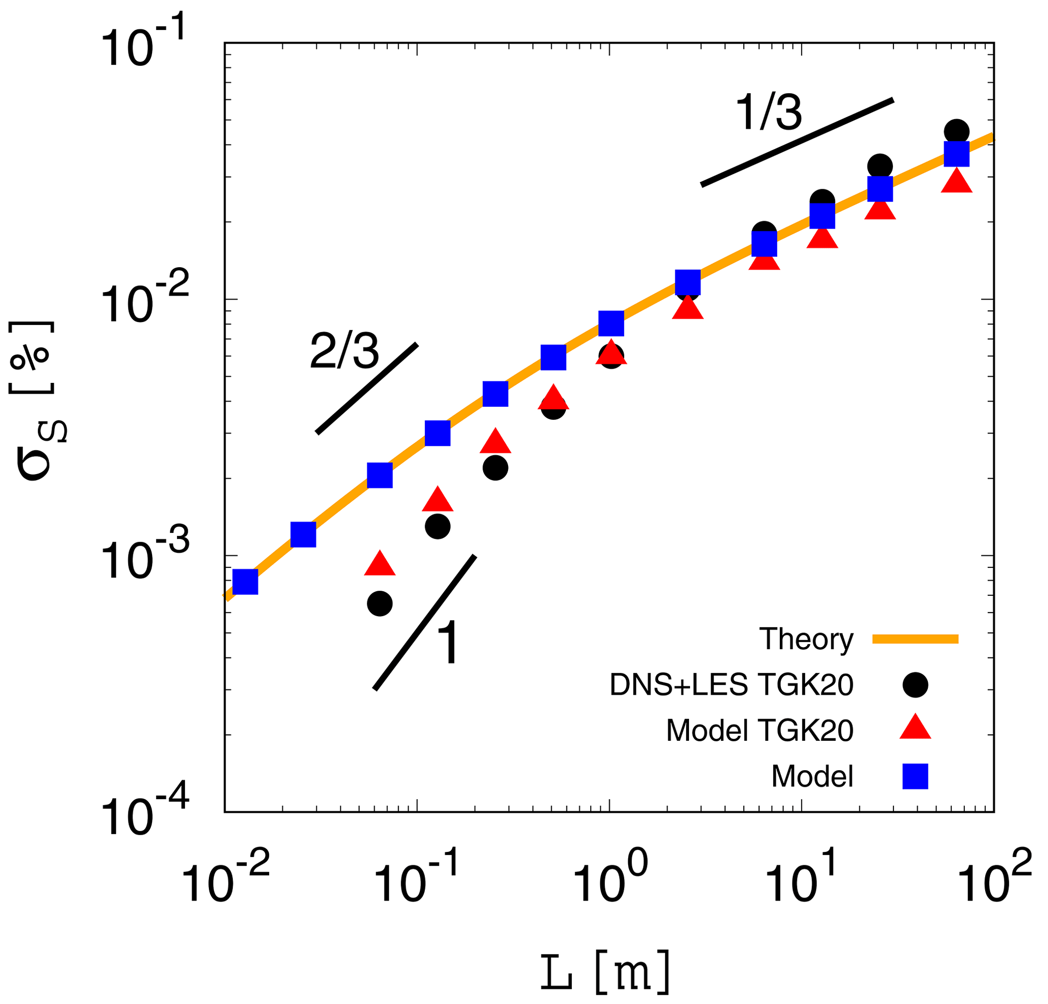
Figure 1 Standard deviation of the supersaturation fluctuation ${\mathit{\sigma }}_{S^{\prime }}$ in the statistically steady state obtained from the analytical expression given by Eq. (13) (orange curve) and the results of our numerical integration of the original version of the eddy-hopping model (blue squares). The horizontal axis is the integral length L. The black dots indicate the reference data taken from direct numerical simulations and large-eddy simulations by Thomas et al. (2020). The red triangles indicate the results of the numerical integration of the original version reported by Thomas et al. (2020). The range of L and ${\mathit{\sigma }}_{S^{\prime }}$ for the panel is the same as in Fig. 10 in Thomas et al. (2020). The three short black lines indicate slopes of 1, $\mathrm{2}/\mathrm{3}$, and $\mathrm{1}/\mathrm{3}$.

Figure 1 compares the scale dependence of ${\mathit{\sigma }}_{S^{\prime }}$ for the analytical expression given by Eq. (13) (orange curve) with the results of the numerical integration of the original version given by Eqs. (1) and (2) (blue squares). Here, numerical integration is conducted in the same manner as that by Thomas et al. (2020) (Sect. 5 of their study), except that the integration time is increased from 6τ to 10τ (see Appendix A for details). After the integration time of 10τ, all of the experimental results achieved a statistically steady state and agreed with the theoretical curve (compare the orange curve and the blue squares). As expected based on the analysis, the theoretical curve shows the scaling ${\mathit{\sigma }}_{S^{\prime }}\sim L^{\mathrm{1}/\mathrm{3}}$ for large scales (approximately L>10¹m) and the improper scaling ${\mathit{\sigma }}_{S^{\prime }}\sim L^{\mathrm{2}/\mathrm{3}}$ for small scales (approximately $L<{\mathrm{10}}^{-\mathrm{1}}$m). These results are contrary to the results of DNSs and LESs (scaled-up DNSs) conducted by Thomas et al. (2020) (black dots in Fig. 1), which show the proper scalings both for large and small scales (${\mathit{\sigma }}_{S^{\prime }}\sim L^{\mathrm{1}/\mathrm{3}}$ and ∼L¹, respectively).

Note that Fig. 1 also shows the results of the numerical integration of the original version reported by Thomas et al. (2020) (red triangles), and their results disagree with the results of the present study. A possible reason for this discrepancy might be that their results did not achieve a statistically steady state. For details, see Appendix C.

The original version of the eddy-hopping model given by Eqs. (1) and (2) shows the improper scaling for small scales because of the assumption made in the formulation of the model. Originally, Eq. (2) (corresponding to Eq. 8 in Grabowski and Abade, 2017) was formulated under the assumption of large scales (or Da≫1), since this assumption usually holds for typical situations in atmospheric clouds. Thus, it is reasonable that the original version does not reproduce the proper scaling for small scales.

4 Statistical properties of the second version

We next consider the second version of the eddy-hopping model by Abade et al. (2018), which is written as follows:

$$\begin{array}{}\text{(18)}& {\displaystyle }{w}^{\prime }(t+\mathit{\delta }t)& {\displaystyle }=w^{\prime }\left(t\right){\mathrm{e}}^{-\mathit{\delta }t/\left(c_{\mathrm{1}}\mathit{\tau }\right)}+\sqrt{\mathrm{1}-{\mathrm{e}}^{-\frac{\mathrm{2}\mathit{\delta }t}{\left(c_{\mathrm{1}}\mathit{\tau }\right)}}}{\mathit{\sigma }}_{w^{\prime }}\mathit{\psi },\text{(19)}& {\displaystyle \frac{\mathrm{d}{S}^{\prime }}{\mathrm{d}t}}& {\displaystyle }=a_{\mathrm{1}}{w}^{\prime }-{\displaystyle \frac{S^{\prime }}{\left(c_{\mathrm{2}}{\mathit{\tau }}_{\mathrm{relax}}\right)}}-{\displaystyle \frac{S^{\prime }}{\left(c_{\mathrm{1}}\mathit{\tau }\right)}}.\end{array}$$

Note that, for subsequent use, we write the governing equations in a slightly generalized form by introducing two parameters c₁ and c₂. The second version by Abade et al. (2018) has $c_{\mathrm{1}}=c_{\mathrm{2}}=\mathrm{1}$.

The important change introduced by Abade et al. (2018) into the original version is the term proportional to $-S^{\prime }/\mathit{\tau }$ in Eq. (19). Physically, this term represents the damping effect on S^′ due to turbulent mixing (eddy diffusivity). This type of term is commonly included in stochastic models used in cloud turbulence research (Sardina et al., 2015, 2018; Chandrakar et al., 2016; Siewert et al., 2017; Saito et al., 2019a). The timescale of the damping effect due to turbulent mixing is characterized by the integral time τ, whereas that due to condensation or evaporation of cloud droplets is characterized by the phase relaxation time τ_relax. The relative importance of these two effects is characterized by the Damköhler number ($Da=\mathit{\tau }/{\mathit{\tau }}_{\mathrm{relax}}$), where the damping effect due to turbulent mixing is dominant for Da≪1 (corresponding to small scales). Below we show that the term $-S^{\prime }/\mathit{\tau }$ plays an essential role in reproducing the proper scaling.

Note that it is possible to further extend the second version by additionally introducing the Wiener process term representing small-scale fluctuations or mixing into Eq. (19) for the supersaturation fluctuation. Readers are referred to Paoli and Shariff (2009) and Sardina et al. (2015) for the Langevin model including such terms, and also to Chandrakar et al. (2021), who implemented such a Langevin model into the LES Lagrangian cloud model and investigated the impact of entrainment mixing and turbulent fluctuations on droplet size distributions in a cumulus cloud. In the present study, however, we focus on statistical properties of the second version with Eqs. (18) and (19).

Applying the analytical procedure described in Sect. 3 to the second version given by Eqs. (18) and (19), we first obtain

$$\begin{array}{ll}{\displaystyle }\langle w^{\prime }{S}^{\prime }\rangle & {\displaystyle }=a_{\mathrm{1}}{\left({\displaystyle \frac{\mathrm{2}}{c_{\mathrm{1}}\mathit{\tau }}}+{\displaystyle \frac{\mathrm{1}}{c_{\mathrm{2}}{\mathit{\tau }}_{\mathrm{relax}}}}\right)}^{-\mathrm{1}}{\mathit{\sigma }}_{w^{\prime }}^{\mathrm{2}}\\ \text{(20)}& {\displaystyle }& {\displaystyle }=c_{\mathrm{1}}{a}_{\mathrm{1}}[\mathrm{2}+(c_{\mathrm{1}}/c_{\mathrm{2}})Da{]}^{-\mathrm{1}}\mathit{\tau }{\mathit{\sigma }}_{w^{\prime }}^{\mathrm{2}},\end{array}$$

instead of Eq. (8). Next, instead of Eq. (11), we have

$$\begin{array}{ll}{\displaystyle }{\mathit{\sigma }}_{S^{\prime }}^{\mathrm{2}}=\langle {S^{\prime }}^{\mathrm{2}}\rangle & {\displaystyle }=a_{\mathrm{1}}{\left({\displaystyle \frac{\mathrm{1}}{c_{\mathrm{1}}\mathit{\tau }}}+{\displaystyle \frac{\mathrm{1}}{c_{\mathrm{2}}{\mathit{\tau }}_{\mathrm{relax}}}}\right)}^{-\mathrm{1}}\langle w^{\prime }{S}^{\prime }\rangle \\ \text{(21)}& {\displaystyle }& {\displaystyle }=c_{\mathrm{1}}{a}_{\mathrm{1}}[\mathrm{1}+(c_{\mathrm{1}}/c_{\mathrm{2}})Da{]}^{-\mathrm{1}}\mathit{\tau }\langle w^{\prime }{S}^{\prime }\rangle .\end{array}$$

Finally, the analytical expression corresponding to Eq. (13) is

$$\begin{array}{}\text{(22)}& {\displaystyle }{\mathit{\sigma }}_{S^{\prime }}=[\mathrm{1}+(c_{\mathrm{1}}/c_{\mathrm{2}}\left)Da{]}^{-\mathrm{1}/\mathrm{2}}\right[\mathrm{2}+(c_{\mathrm{1}}/c_{\mathrm{2}})Da{]}^{-\mathrm{1}/\mathrm{2}}{c}_{\mathrm{1}}{a}_{\mathrm{1}}\mathit{\tau }{\mathit{\sigma }}_{w^{\prime }}.\end{array}$$

Asymptotic forms of ${\mathit{\sigma }}_{S^{\prime }}$ in Eq. (22) for the large and small scale limits are, respectively, given as follows:

1. Large scale limit.
   For τ→∞ (or equivalently, Da→∞, L→∞), ${\mathit{\sigma }}_{S^{\prime }}$ in Eq. (22) is approximated as

   $$\begin{array}{ll}{\displaystyle }{\mathit{\sigma }}_{S^{\prime }}& {\displaystyle }\approx c_{\mathrm{2}}{a}_{\mathrm{1}}D{a}^{-\mathrm{1}}\mathit{\tau }{\mathit{\sigma }}_{w^{\prime }}\\ \text{(23)}& {\displaystyle }& {\displaystyle }=c_{\mathrm{2}}{a}_{\mathrm{1}}{\mathit{\tau }}_{\mathrm{relax}}{\mathit{\sigma }}_{w^{\prime }}.\end{array}$$

   For the case of a constant dissipation rate of turbulent kinetic energy ε, we have

   $$\begin{array}{}\text{(24)}& {\displaystyle }{\mathit{\sigma }}_{S^{\prime }}\sim L^{\mathrm{1}/\mathrm{3}}.\end{array}$$

2. Small scale limit.
   For τ→0 (or equivalently, Da→0, L→0), ${\mathit{\sigma }}_{S^{\prime }}$ in Eq. (22) is approximated as

   $$\begin{array}{}\text{(25)}& {\displaystyle }{\mathit{\sigma }}_{S^{\prime }}\approx {\mathrm{2}}^{-\mathrm{1}/\mathrm{2}}{c}_{\mathrm{1}}{a}_{\mathrm{1}}\mathit{\tau }{\mathit{\sigma }}_{w^{\prime }},\end{array}$$

   which indicates that ${\mathit{\tau }}_{\mathrm{relax}}^{\mathrm{1}/\mathrm{2}}$ in Eq. (16) has been replaced by ${\mathit{\tau }}^{\mathrm{1}/\mathrm{2}}$ by introducing the term $-S^{\prime }/\mathit{\tau }$ in Eq. (19). For the case of a constant dissipation rate of turbulent kinetic energy ε, we have

   $$\begin{array}{}\text{(26)}& {\displaystyle }{\mathit{\sigma }}_{S^{\prime }}\sim L.\end{array}$$

Therefore, the second version successfully reproduces asymptotic forms ${\mathit{\sigma }}_{S^{\prime }}\sim a_{\mathrm{1}}{\mathit{\tau }}_{\mathrm{relax}}{\mathit{\sigma }}_{w^{\prime }}$ and $\sim a_{\mathrm{1}}\mathit{\tau }{\mathit{\sigma }}_{w^{\prime }}$ for the large and small scale limits, respectively, which are both consistent with the result of the scaling argument by Lanotte et al. (2009).

Figure 2 Standard deviation of the supersaturation fluctuation ${\mathit{\sigma }}_{S^{\prime }}$ in the statistically steady state obtained from the analytical expression given by Eq. (22) for the second version ($c_{\mathrm{1}}=c_{\mathrm{2}}=\mathrm{1}$, orange curve) and the results of our numerical integration using the second version given by Eqs. (18) and (19) ($c_{\mathrm{1}}=c_{\mathrm{2}}=\mathrm{1}$, green diamonds). The dashed line indicates the analytical expression given by Eq. (13) for the original version. The two short black lines indicate slopes of 1 and $\mathrm{1}/\mathrm{3}$. The black dots and the axes of the panel are the same as in Fig. 1.

Figure 2 (orange curve) shows the theoretical curve given by Eq. (22) for the second version ($c_{\mathrm{1}}=c_{\mathrm{2}}=\mathrm{1}$). The second version reproduces the proper scalings both for large and small scales (${\mathit{\sigma }}_{S^{\prime }}\sim L^{\mathrm{1}/\mathrm{3}}$ and ∼L¹, respectively) and demonstrates better agreement with the reference data (black dots) than the original version for L<10⁰ m. Figure 2 (green diamonds) also shows the results of the numerical integration of the second version, which agree with the theoretical curve (orange curve), as expected. Here, the numerical integration was conducted in the same manner as in the previous section (see Appendix A for details).

Figure 3 Standard deviation of the supersaturation fluctuation ${\mathit{\sigma }}_{S^{\prime }}$ in the statistically steady state from the analytical expression (22) for the second version. The dashed curve is for $c_{\mathrm{1}}=c_{\mathrm{2}}=\mathrm{1}$, and the solid curve is for c₁=0.746 and c₂=1.28. The black dots and the axes of the panel are the same as in Fig. 1.

Although improved, the second version still slightly over- and underestimates the supersaturation fluctuations for $L<\mathrm{3}\times {\mathrm{10}}^{-\mathrm{1}}$ and $L>\mathrm{2}\times {\mathrm{10}}^{\mathrm{0}}$ m, respectively, as shown in Fig. 2 (compare the orange curve with black dots). This deviation from the reference data can be further reduced by adjusting two parameters c₁ and c₂ in Eqs. (18) and (19). The analytical expression (22) and its asymptotic forms (23) and (25) show how c₁ and c₂ work. These types of parameters are not new. For example, a parameter corresponding to c₁ is commonly used in the Langevin stochastic equation in turbulence research (Sawford, 1991; Marcq and Naert, 1998). Formally, the inverse of c₁ is referred to as the drift coefficient, and the coefficients for the velocity and scalar equations should be distinguished. However, we treat these coefficients as the same parameter in Eqs. (18) and (19) for simplicity. On the other hand, the importance of a parameter corresponding to c₂ has been demonstrated in a recent study on turbulence modulation by particles (Saito et al., 2019b).

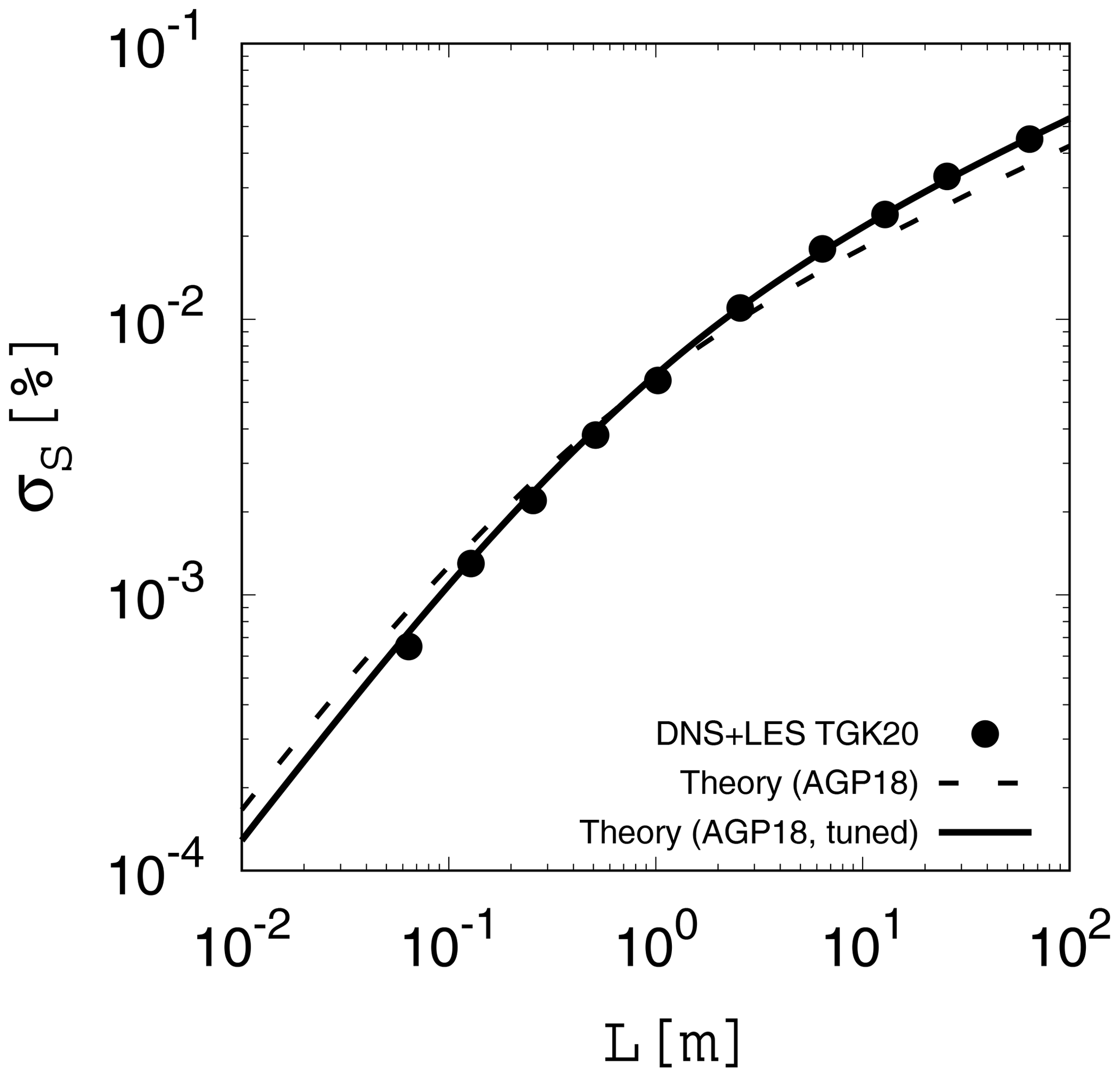
Here, we do not consider any physical meaning for c₁ and c₂ and use them just as tuning parameters. Two parameters c₁ and c₂ are determined by comparing the theoretical curve given by Eq. (22) with the reference data taken from DNSs and LESs in Thomas et al. (2020). The best fit is given by c₁=0.746 and c₂=1.28. Figure 3 (solid curve) shows the theoretical curve given by Eq. (22) with these values of c₁ and c₂, which agrees almost perfectly with the reference data (black dots). Although the improvement from the second version with $c_{\mathrm{1}}=c_{\mathrm{2}}=\mathrm{1}$ is slight, this result shows that the eddy-hopping model can be easily tuned to reproduce the reference data almost perfectly.

5 Possibility of simplification of the model

Finally, we discuss the possibility of simplification of the eddy-hopping model. Here, our discussion is based on the second version given by Eqs. (18) and (19), but the same argument also applies to the original version given by Eqs. (1) and (2).

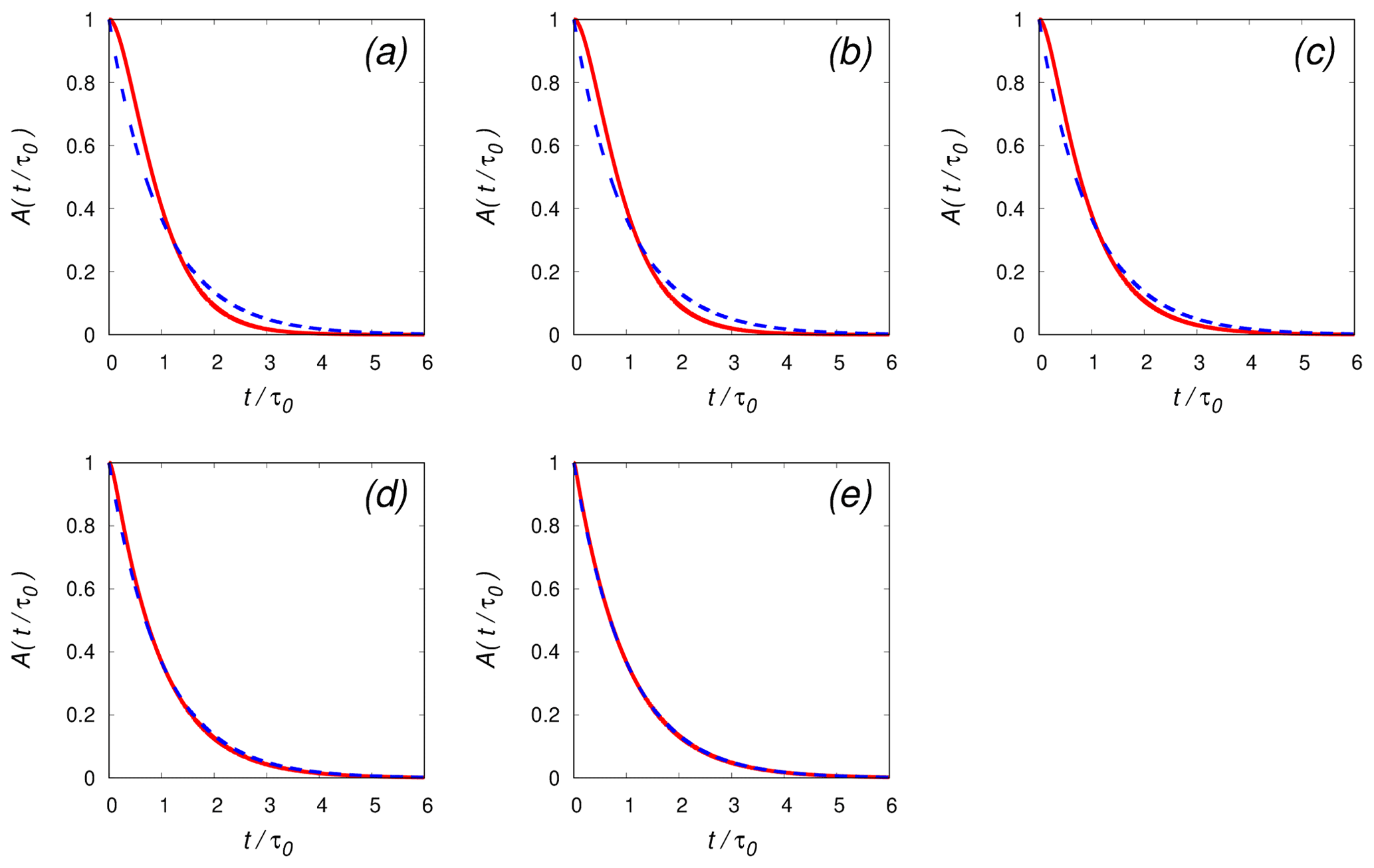
Figure 4 Auto-correlation functions in the statistically steady state for the simplified model (B(t) in Eq. 35: blue dashed curve) and the second version (A(t) in Eq. 28: red solid curve). Here, $c_{\mathrm{1}}=c_{\mathrm{2}}=\mathrm{1}$. The parameters for each panel are as follows: (a) $L={\mathrm{10}}^{-\mathrm{2}}$ m, τ=0.447 s, τ₀=0.844 s, Da=0.127; (b) $L={\mathrm{10}}^{-\mathrm{1}}$ m, τ=2.08 s, τ₀=3.38 s, Da=0.591; (c) L=10⁰ m, τ=9.63 s, τ₀=12.2 s, Da=2.74; (d) L=10¹ m, τ=44.7 s, τ₀=48.0 s, Da=12.7; and (e) L=10² m, τ=208 s, τ₀=211 s, Da=59.1. The phase relaxation time is fixed to τ_relax=3.513 s. The horizontal axis is the time t normalized by the auto-correlation time τ₀ for each case. The parameter τ is determined from the integral length L based on the setting for the numerical experiment described in Appendices A and B.

The eddy-hopping model consists of two evolution equations for the supersaturation and vertical velocity fluctuations, S^′ and w^′ respectively, and these two variables fluctuate randomly according to the Ornstein–Uhlenbeck process. However, if we have S^′ that fluctuates with a proper amplitude and auto-correlation function, then we do not need the evolution equation for w^′, because only S^′ is used in the growth equation of the droplet size. As described in Sect. 4, we obtained an analytical expression for ${\mathit{\sigma }}_{S^{\prime }}$, i.e., the standard deviation of the supersaturation fluctuation in the statistically steady state given by Eq. (22). On the other hand, the auto-correlation function for S^′ in a statistically steady state can also be obtained analytically. The derivation is described in Appendix D. The result is given in Eq. (D14) and is as follows:

$$\begin{array}{}\text{(27)}& {\displaystyle }A\left(t\right)& {\displaystyle }={\displaystyle \frac{〈S^{\prime }(t+t_{\mathrm{0}})S^{\prime }\left(t_{\mathrm{0}}\right)〉}{〈S^{\prime }\left(t_{\mathrm{0}}\right)S^{\prime }\left(t_{\mathrm{0}}\right)〉}}\text{(28)}& {\displaystyle }& {\displaystyle }=\left({\displaystyle \frac{{\mathit{\tau }}_{\mathrm{1}}}{{\mathit{\tau }}_{\mathrm{1}}-{\mathit{\tau }}_{\mathrm{2}}}}\right){\mathrm{e}}^{-t/{\mathit{\tau }}_{\mathrm{1}}}-\left({\displaystyle \frac{{\mathit{\tau }}_{\mathrm{2}}}{{\mathit{\tau }}_{\mathrm{1}}-{\mathit{\tau }}_{\mathrm{2}}}}\right){\mathrm{e}}^{-t/{\mathit{\tau }}_{\mathrm{2}}},\end{array}$$

where τ₁ and τ₂ are, respectively, defined as

$$\begin{array}{}\text{(29)}& \begin{array}{rl}{\mathit{\tau }}_{\mathrm{1}}& =c_{\mathrm{1}}\mathit{\tau },\mathrm{and}{\mathit{\tau }}_{\mathrm{2}}={\left({\displaystyle \frac{\mathrm{1}}{c_{\mathrm{1}}\mathit{\tau }}}+{\displaystyle \frac{\mathrm{1}}{c_{\mathrm{2}}{\mathit{\tau }}_{\mathrm{relax}}}}\right)}^{-\mathrm{1}}\\ & =c_{\mathrm{1}}\mathit{\tau }{\left(\mathrm{1}+{\displaystyle \frac{c_{\mathrm{1}}}{c_{\mathrm{2}}}}Da\right)}^{-\mathrm{1}}.\end{array}\end{array}$$

We can also obtain the auto-correlation time for S^′ by time integration of A(t) (see Eq. D16 in Appendix D), which is given as

$$\begin{array}{}\text{(30)}& {\displaystyle }{\mathit{\tau }}_{\mathrm{0}}={\mathit{\tau }}_{\mathrm{1}}+{\mathit{\tau }}_{\mathrm{2}}.\end{array}$$

The auto-correlation function A(t) in Eq. (28) and the auto-correlation time τ₀ in Eq. (30), with τ₁ and τ₂ defined by (29), have important asymptotic forms in two limits. First, for the large scale limit (Da→∞), the asymptotic forms of A(t) and τ₀ are given by

$$\begin{array}{}\text{(31)}& {\displaystyle }\underset{Da\to \mathrm{\infty }}{lim}A\left(t\right)={\mathrm{e}}^{-t/\left(c_{\mathrm{1}}\mathit{\tau }\right)}\mathrm{and}\underset{Da\to \mathrm{\infty }}{lim}{\mathit{\tau }}_{\mathrm{0}}=c_{\mathrm{1}}\mathit{\tau },\end{array}$$

respectively. Second, for the small scale limit (Da→0), the asymptotic forms of A(t) and τ₀ are given by

$$\begin{array}{}\text{(32)}& \begin{array}{rl}& \underset{Da\to \mathrm{0}}{lim}A\left(t\right)=\left[\mathrm{1}+{\displaystyle \frac{t}{\left(c_{\mathrm{1}}\mathit{\tau }\right)}}\right]{\mathrm{e}}^{-t/\left(c_{\mathrm{1}}\mathit{\tau }\right)}\mathrm{and}\\ & \underset{Da\to \mathrm{0}}{lim}{\mathit{\tau }}_{\mathrm{0}}=\mathrm{2}{c}_{\mathrm{1}}\mathit{\tau },\end{array}\end{array}$$

respectively.

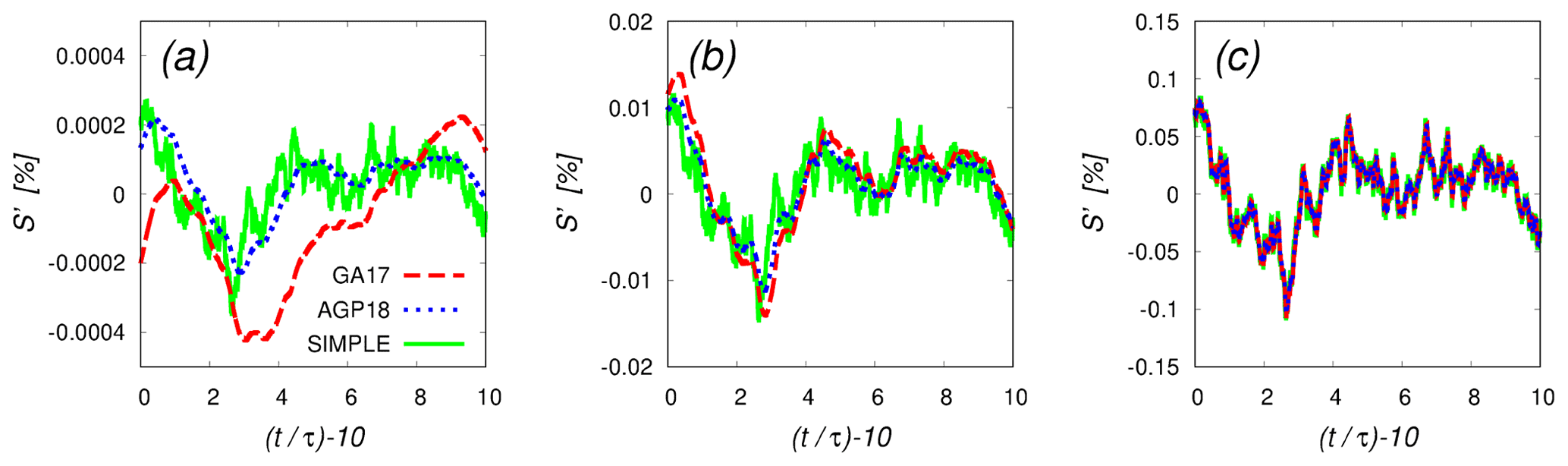
Figure 5 Time evolutions of the supersaturation fluctuations obtained from the numerical integration of the original version (Eqs. 1 and 2, dashed red curve), the second version (Eqs. 18 and 19, dotted blue curve), and the simplified model (Eq. 33, solid green curve). The parameters for each panel are as follows: (a) $L={\mathrm{10}}^{-\mathrm{2}}$ m, τ=0.447 s, Da=0.127; (b) L=10⁰ m, τ=9.63 s, Da=2.74; (c) L=10² m, τ=208 s, Da=59.1. The phase relaxation time is fixed to τ_relax=3.513 s. Results are shown for the time range $\mathrm{0}\le (t/\mathit{\tau }-\mathrm{10})\le \mathrm{10}$ (or equivalently, $\mathrm{10}\mathit{\tau }\le t\le \mathrm{20}\mathit{\tau }$), where all cases are already in a statistically steady state. The numerical integration was conducted in the same manner as described in Appendix A. All results were obtained by using the same random number series.

Based on analytical expressions for the fluctuation amplitude and the auto-correlation function for S^′ (Eqs. 22 and 30, respectively), a simplified version of the eddy-hopping model is defined as follows:

$$\begin{array}{}\text{(33)}& {\displaystyle }{S}^{\prime }(t+\mathit{\delta }t)=S^{\prime }\left(t\right){\mathrm{e}}^{-\mathit{\delta }t/{\mathit{\tau }}_{\mathrm{0}}}+\sqrt{\mathrm{1}-{\mathrm{e}}^{-\frac{\mathrm{2}\mathit{\delta }t}{{\mathit{\tau }}_{\mathrm{0}}}}}{\mathit{\sigma }}_{S^{\prime }}\mathit{\psi },\end{array}$$

where ${\mathit{\sigma }}_{S^{\prime }}$ and τ₀ are given by Eqs. (22) and (30), respectively. Note that the simplified model given by Eq. (33) is a single-equation model, as compared to the two-equation model given by Eqs. (18) and (19) before the simplification. The auto-correlation function for S^′ in the simplified model given by Eq. (33) is as follows:

$$\begin{array}{}\text{(34)}& {\displaystyle }B\left(t\right)& {\displaystyle }={\displaystyle \frac{〈S^{\prime }(t+t_{\mathrm{0}})S^{\prime }\left(t_{\mathrm{0}}\right)〉}{〈S^{\prime }\left(t_{\mathrm{0}}\right)S^{\prime }\left(t_{\mathrm{0}}\right)〉}}\text{(35)}& {\displaystyle }& {\displaystyle }={\mathrm{e}}^{-t/{\mathit{\tau }}_{\mathrm{0}}},\end{array}$$

which has the following two asymptotic forms. First, for the large scale limit (Da→∞),

$$\begin{array}{}\text{(36)}& {\displaystyle }\underset{Da\to \mathrm{\infty }}{lim}B\left(t\right)={\mathrm{e}}^{-t/\left(c_{\mathrm{1}}\mathit{\tau }\right)},\end{array}$$

which agrees with the corresponding asymptotic form given by Eq. (31) for the second version. Second, for the small scale limit (Da→0),

$$\begin{array}{}\text{(37)}& {\displaystyle }\underset{Da\to \mathrm{0}}{lim}B\left(t\right)={\mathrm{e}}^{-t/\left(\mathrm{2}{c}_{\mathrm{1}}\mathit{\tau }\right)},\end{array}$$

which disagrees with the corresponding asymptotic form given by Eq. (32) for the second version.

Figures 4a through e compare the auto-correlation function for the simplified model (B(t) in Eq. 35: blue dashed curve) and that for the second version (A(t) in Eq. 28: red solid curve) for five cases ranging from Da≪1 to Da≫1. Here, $c_{\mathrm{1}}=c_{\mathrm{2}}=\mathrm{1}$. Note that the time t is normalized by the auto-correlation time τ₀ for each case. Although B(t) and A(t) share the same auto-correlation time, B(t) deviates from A(t) for cases with Da of order unity or smaller, as shown in Fig. 4a through c. On the other hand, for Da≫1, B(t) agrees with A(t) very well, as shown in Fig. 4d and e.

The simplified model has the desirable convergence property. The auto-correlation function for the simplified model (B(t) in Eq. 35) converges to that for the second version in the large-scale limit (Da→∞), as shown in Eq. (36). As confirmed in Figs. 4d and e, the two auto-correlation functions are almost identical for an integral length L greater than 10 m (or Da≥10). In the implementation of the eddy-hopping model to the LES Lagrangian cloud model, the integral length L is supposed to roughly correspond to the grid size, which is often greater than several meters to several tens of meters. Therefore, the assumption of large scales (or Da≫1) usually holds, in which case the statistical properties of the simplified model are expected to be almost unchanged after the simplification.

Figure 5 compares the time evolutions of the supersaturation fluctuations obtained from the numerical integration of the original version (dashed red curve), the second version (dotted blue curve), and the simplified model (solid green curve). Here, the numerical integration was conducted in the same manner as described in Appendix A. All results were obtained by using the same random number series. The results are shown in the time range $\mathrm{10}\mathit{\tau }\le t\le \mathrm{20}\mathit{\tau }$, where all cases are already in a statistically steady state.

For small scales, the simplified model produces qualitatively different trajectories of S^′ from the second version, as shown in Fig. 5a ($L={\mathrm{10}}^{-\mathrm{2}}$ m; compare the solid green and dotted blue curves), even though these two models share the same fluctuation amplitude ${\mathit{\sigma }}_{S^{\prime }}$ and the auto-correlation time τ₀ in the statistically steady state. The difference is smaller for intermediate scales (Fig. 5b, L=10⁰ m). For sufficiently large scales (Fig. 5c, L=10² m), the simplified model and the second version produce almost identical results.

6 Summary and conclusions

The purpose of the present paper was to obtain various statistical properties of the eddy-hopping model, a novel cloud microphysical model, which accounts for the effect of the supersaturation fluctuation at unresolved scales on the growth of cloud droplets and on spectral broadening. Two versions of the model are considered: the original version by Grabowski and Abade (2017) and the second version by Abade et al. (2018). Based on derived statistical properties, we first showed in Sect. 3 that the original version fails to reproduce a proper scaling for smaller Damköhler numbers (corresponding to small scales), resulting in a deviation of the model prediction from the reference data taken from DNSs and LESs, as shown in Fig. 1. In Sect. 4, we showed that the second version successfully reproduces the proper scaling and agrees better with the reference data than the original version for small scales (L<10⁰ m in Fig. 2). We also showed that, by adjusting two parameters c₁ and c₂, the second version can almost perfectly reproduce the reference data. In Sect. 5, we discussed the possibility of simplification of the model. The simplified model consists of a single stochastic equation for the supersaturation fluctuation, as in Eq. (33), with amplitude and time parameters given by the corresponding analytical expressions for the model before the simplification. We showed that, for larger Damköhler numbers (corresponding to large scales), the auto-correlation function of the supersaturation fluctuation for the simplified model converges to that for the model before the simplification. This convergence property is desirable because the assumption of large scales usually holds in the typical parameter range for the model implementation in the LES Lagrangian cloud model.

Appendix A: Numerical integration of the eddy-hopping model

The results of the numerical integration of the original version (Eqs. 1 and 2) and the second version (Eqs. 18 and 19) are shown in Figs. 1 (blue squares) and 2 (green diamonds), respectively. For these experiments, we used the same setting as that in Sect. 5 in Thomas et al. (2020), except that the integration time was increased from 6τ to 10τ. We set $a_{\mathrm{1}}=\mathrm{4.753}\times {\mathrm{10}}^{-\mathrm{4}}$ m⁻¹, ε=10 cm² s⁻³, and τ_relax=3.513 s, and the integral time τ as

$$\begin{array}{}\text{(A1)}& {\displaystyle }\mathit{\tau }={\displaystyle \frac{\mathrm{1}}{(\mathrm{2}\mathit{\pi }{)}^{\mathrm{1}/\mathrm{3}}}}\left({\displaystyle \frac{L}{{\mathit{\sigma }}_{w^{\prime }}}}\right).\end{array}$$

As described in Appendix B, for the case of a constant dissipation rate of turbulent kinetic energy ε, ${\mathit{\sigma }}_{w^{\prime }}$ is given as a function of L. We time integrated the governing equations of the model using 12 values of L: L=0.0128, 0.0256, 0.064, 0.128, 0.256, 0.512, 1.024, 2.56, 6.4, 12.8, 25.6, and 64.0 m. The time step δt is set as $\mathrm{1}/\mathrm{1000}$ of τ, and the integration time is 10τ. The numerical scheme is the forward Euler method. The initial condition is such that $w^{\prime }\left(\mathrm{0}\right)={\mathit{\sigma }}_{w^{\prime }}\mathit{\psi }$ and $S^{\prime }\left(\mathrm{0}\right)=\mathrm{0}$. Each result in Figs. 1 (blue squares) and 2 (green diamonds) is obtained by averaging the results for 1000 ensembles with different seeds of random numbers.

Appendix B: Scalings for the case of a constant dissipation rate of turbulent kinetic energy

We consider classical homogeneous isotropic turbulence, in which energy is mainly injected into the system at large scales, cascaded to smaller scales by nonlinear interaction, and finally dissipated by the molecular viscosity in the smallest scales. In a statistically steady state, the dissipation rate of turbulent kinetic energy is defined as ε. If ε is fixed and the integral scale L is changed, then the kinetic energy E scales as follows (Thomas et al., 2020):

$$\begin{array}{}\text{(B1)}& E\sim (L\mathit{\epsilon }{)}^{\mathrm{2}/\mathrm{3}}.\end{array}$$

The black dots in Fig. B1 show the relation between L and E in the reference data taken from DNSs and LESs by Thomas et al. (2020) (Table 2 of their study). In their simulation, the dissipation rate was fixed to ε=10 cm²s⁻³. The orange curve in Fig. B1 indicates the function $E=\mathit{\alpha }{\mathit{\epsilon }}^{\mathrm{2}/\mathrm{3}}{L}^{\mathrm{2}/\mathrm{3}}$, where α is the fitting parameter. The best fit is given by α=0.475. The root-mean-square turbulent velocity is calculated as a function of L by $u_{\mathrm{rms}}={\mathit{\sigma }}_{w^{\prime }}=\sqrt{(\mathrm{2}E/\mathrm{3})}$, and ${\mathit{\sigma }}_{w^{\prime }}$ is used as the parameter in the eddy-hopping model. Note that Thomas et al. (2020) used the same type of large-scale forcing as that used by Kumar et al. (2012), where the integral length L is set to be equal to the box length L_box.

Figure B1 Relationship between the integral scale L and the turbulent kinetic energy E. The black dots are taken from the reference data in Thomas et al. (2020). The orange curve indicates the fitting function $E=\mathit{\alpha }{\mathit{\epsilon }}^{\mathrm{2}/\mathrm{3}}{L}^{\mathrm{2}/\mathrm{3}}$ with α=0.475.

Appendix C: Achievement of a statistically steady state

We confirm that all of the results of the numerical integration of the eddy-hopping model in the present study achieved statistically steady states. For this purpose, we first derive the analytical expression for the time evolutions of the variance and covariance of the variables in the model and then compare these analytical expressions with the results of the numerical integration.

The governing equations given by Eqs. (3) and (2) can be rewritten in generalized forms as

$$\begin{array}{}\text{(C1)}& {\displaystyle \frac{\mathrm{d}{w}^{\prime }}{\mathrm{d}t}}& {\displaystyle }=-{\displaystyle \frac{\mathrm{1}}{{\mathit{\tau }}_{\mathrm{1}}}}{w}^{\prime }\left(t\right)+F_{w^{\prime }}\left(t\right),\text{(C2)}& {\displaystyle \frac{\mathrm{d}{S}^{\prime }}{\mathrm{d}t}}& {\displaystyle }=a_{\mathrm{1}}{w}^{\prime }\left(t\right)-{\displaystyle \frac{S^{\prime }\left(t\right)}{{\mathit{\tau }}_{\mathrm{2}}}},\end{array}$$

where τ₁ and τ₂ are the relaxation times for w^′ and S^′, respectively, and the forcing term $F_{w^{\prime }}\left(t\right)$ satisfies Eq. (4). Evolution equations for the variance and covariance of the variables are derived as follows:

$$\begin{array}{}\text{(C3)}& {\displaystyle \frac{\mathrm{d}{V}_{w^{\prime }}\left(t\right)}{\mathrm{d}t}}& {\displaystyle }=-{\displaystyle \frac{\mathrm{2}}{{\mathit{\tau }}_{\mathrm{1}}}}{V}_{w^{\prime }}\left(t\right)+\left({\displaystyle \frac{\mathrm{2}{\mathit{\sigma }}_{w^{\prime }}^{\mathrm{2}}}{{\mathit{\tau }}_{\mathrm{1}}}}\right),\text{(C4)}& {\displaystyle \frac{\mathrm{d}C\left(t\right)}{\mathrm{d}t}}& {\displaystyle }=a_{\mathrm{1}}{V}_{w^{\prime }}\left(t\right)-\left({\displaystyle \frac{\mathrm{1}}{{\mathit{\tau }}_{\mathrm{1}}}}+{\displaystyle \frac{\mathrm{1}}{{\mathit{\tau }}_{\mathrm{2}}}}\right)C\left(t\right),\text{(C5)}& {\displaystyle \frac{\mathrm{d}{V}_{S^{\prime }}\left(t\right)}{\mathrm{d}t}}& {\displaystyle }=-{\displaystyle \frac{\mathrm{2}}{{\mathit{\tau }}_{\mathrm{2}}}}{V}_{S^{\prime }}\left(t\right)+\mathrm{2}{a}_{\mathrm{1}}C\left(t\right),\end{array}$$

where $V_{w^{\prime }}\left(t\right)$, C(t), and $V_{S^{\prime }}\left(t\right)$ are, respectively, defined as

$$\begin{array}{}\text{(C6)}& {\displaystyle }{V}_{w^{\prime }}\left(t\right)& {\displaystyle }=〈w^{\prime }\left(t\right)w^{\prime }\left(t\right)〉,\text{(C7)}& {\displaystyle }C\left(t\right)& {\displaystyle }=〈w^{\prime }\left(t\right)S^{\prime }\left(t\right)〉,\text{(C8)}& {\displaystyle }{V}_{S^{\prime }}\left(t\right)& {\displaystyle }=〈S^{\prime }\left(t\right)S^{\prime }\left(t\right)〉.\end{array}$$

For the numerical integration of the eddy-hopping model by Thomas et al. (2020), τ₁=τ and τ₂=τ_relax. Since the initial conditions for w^′(t) and S^′(t) are set to $w^{\prime }\left(\mathrm{0}\right)={\mathit{\sigma }}_{w^{\prime }}\mathit{\psi }$ and $S^{\prime }\left(\mathrm{0}\right)=\mathrm{0}$ in Thomas et al. (2020), the corresponding initial conditions for the variance and covariance are given by

$$\begin{array}{}\text{(C9)}& {\displaystyle }{V}_{w^{\prime }}\left(\mathrm{0}\right)& {\displaystyle }={\mathit{\sigma }}_{w^{\prime }}^{\mathrm{2}},\text{(C10)}& {\displaystyle }C\left(\mathrm{0}\right)& {\displaystyle }=\mathrm{0},\text{(C11)}& {\displaystyle }{V}_{S^{\prime }}\left(\mathrm{0}\right)& {\displaystyle }=\mathrm{0}.\end{array}$$

Solving Eqs. (C3) through (C5) with the initial conditions given by Eqs. (C9) through (C11), we obtain

$$\begin{array}{}\text{(C12)}& {\displaystyle }{V}_{w^{\prime }}\left(t\right)={\mathit{\sigma }}_{w^{\prime }}^{\mathrm{2}},\text{(C13)}& {\displaystyle }C\left(t\right)=a_{\mathrm{1}}{\mathit{\sigma }}_{w^{\prime }}^{\mathrm{2}}{\mathit{\tau }}_{\mathrm{3}}\left(\mathrm{1}-{\mathrm{e}}^{-t/{\mathit{\tau }}_{\mathrm{3}}}\right),\text{(C14)}& {\displaystyle }\begin{array}{rl}{V}_{S^{\prime }}\left(t\right)& =a_{\mathrm{1}}^{\mathrm{2}}{\mathit{\sigma }}_{w^{\prime }}^{\mathrm{2}}{\mathit{\tau }}_{\mathrm{3}}{\mathit{\tau }}_{\mathrm{2}}\left(\mathrm{1}-{\mathrm{e}}^{-\mathrm{2}t/{\mathit{\tau }}_{\mathrm{2}}}\right)\\ & +\mathrm{2}{a}_{\mathrm{1}}^{\mathrm{2}}{\mathit{\sigma }}_{w^{\prime }}^{\mathrm{2}}{\mathit{\tau }}_{\mathrm{3}}{\mathit{\tau }}_{\mathrm{4}}\left({\mathrm{e}}^{-t/{\mathit{\tau }}_{\mathrm{3}}}-{\mathrm{e}}^{-\mathrm{2}t/{\mathit{\tau }}_{\mathrm{2}}}\right),\end{array}\end{array}$$

where τ₃ and τ₄ are, respectively, defined as

$$\begin{array}{}\text{(C15)}& {\displaystyle }{\mathit{\tau }}_{\mathrm{3}}={\displaystyle \frac{{\mathit{\tau }}_{\mathrm{1}}{\mathit{\tau }}_{\mathrm{2}}}{{\mathit{\tau }}_{\mathrm{1}}+{\mathit{\tau }}_{\mathrm{2}}}},\mathrm{and}{\mathit{\tau }}_{\mathrm{4}}={\displaystyle \frac{{\mathit{\tau }}_{\mathrm{1}}{\mathit{\tau }}_{\mathrm{2}}}{{\mathit{\tau }}_{\mathrm{2}}-{\mathit{\tau }}_{\mathrm{1}}}}.\end{array}$$

Figure C1 Standard deviation of the supersaturation fluctuation ${\mathit{\sigma }}_{S^{\prime }}$ at times t=0.6τ (a) and t=6τ (b) obtained from the analytical expression given by Eq. (C14) (cyan dots) and the results of the numerical integration of the original version given by Eqs. (1) and (2) (black crosses). The orange curve, red triangles, and axes of the panel are the same as in Fig. 1. The two short black lines indicate slopes of $\mathrm{2}/\mathrm{3}$ and $\mathrm{1}/\mathrm{3}$. The setting for the numerical integration is the same as that used in Sect. 3, except that the integration times are 0.6τ and 6τ in (a) and (b), respectively.

Figure C1 compares the analytical expression given by Eq. (C14) (cyan dots) with the results of the numerical integration of the original version given by Eqs. (1) and (2) (black crosses). The setting for the numerical experiment is the same as that used in Fig. 1, except that the integration time is 0.6τ in Fig. C1a and 6τ in Fig. C1b. The results of the numerical integration (black crosses) agree well with the analytical expression (cyan dots), and both approach the theoretical curve for the statistically steady state (orange curve in each panel) as the integration time increases. Figure C1a also indicates that the results of the numerical integration of the eddy-hopping model by Thomas et al. (2020) (red triangles) are fairly close to our results at 0.6τ. Thus, it might be possible that the integration time of their numerical experiment was not long enough to achieve a statistically steady state.

Appendix D: Derivation of auto-correlation function

We derive the analytical expression for the auto-correlation function of the supersaturation fluctuation S^′(t) in the eddy-hopping model. As in Appendix C, we start from the generalized form of the eddy-hopping model as follows:

$$\begin{array}{}\text{(D1)}& {\displaystyle \frac{\mathrm{d}{w}^{\prime }}{\mathrm{d}t}}& {\displaystyle }=-{\displaystyle \frac{\mathrm{1}}{{\mathit{\tau }}_{\mathrm{1}}}}{w}^{\prime }\left(t\right)+F_{w^{\prime }}\left(t\right),\text{(D2)}& {\displaystyle \frac{\mathrm{d}{S}^{\prime }}{\mathrm{d}t}}& {\displaystyle }=a_{\mathrm{1}}{w}^{\prime }\left(t\right)-{\displaystyle \frac{S^{\prime }\left(t\right)}{{\mathit{\tau }}_{\mathrm{2}}}},\end{array}$$

where τ₁ and τ₂ are the relaxation times for w^′ and S^′, respectively, and the forcing term $F_{w^{\prime }}\left(t\right)$ satisfies Eq. (4). We consider that the system is in a statistically steady state.

First, multiplying Eq. (D2) by ${\mathrm{e}}^{t/{\mathit{\tau }}_{\mathrm{2}}}$ and applying the product rule of differentiation, we obtain

$$\begin{array}{}\text{(D3)}& {\displaystyle \frac{\mathrm{d}}{\mathrm{d}t}}\left(S^{\prime }\left(t\right){\mathrm{e}}^{t/{\mathit{\tau }}_{\mathrm{2}}}\right)=a_{\mathrm{1}}{w}^{\prime }\left(t\right){\mathrm{e}}^{t/{\mathit{\tau }}_{\mathrm{2}}}.\end{array}$$

Integrating Eq. (D3) from t=0 to t, we obtain

$$\begin{array}{}\text{(D4)}& {\displaystyle }{S}^{\prime }\left(t\right)=S^{\prime }\left(\mathrm{0}\right){\mathrm{e}}^{-t/{\mathit{\tau }}_{\mathrm{2}}}+\underset{\mathrm{0}}{\overset{t}{\int }}{a}_{\mathrm{1}}{w}^{\prime }\left(\mathit{\xi }\right){\mathrm{e}}^{(\mathit{\xi }-t)/{\mathit{\tau }}_{\mathrm{2}}}\mathrm{d}\mathit{\xi }.\end{array}$$

(Note that we chose the integration range [0,t] for simplicity of notation. Since we consider a statistically steady state, the following discussion is unchanged if the integration range is $[t_{\mathrm{0}},t_{\mathrm{0}}+t]$.) Applying a similar procedure to that above to Eq. (D1) with the integration range $t:\mathrm{0}\to \mathit{\xi }$, we obtain

$$\begin{array}{}\text{(D5)}& {\displaystyle }{w}^{\prime }\left(\mathit{\xi }\right)=w^{\prime }\left(\mathrm{0}\right){\mathrm{e}}^{-\mathit{\xi }/{\mathit{\tau }}_{\mathrm{1}}}+\underset{\mathrm{0}}{\overset{\mathit{\xi }}{\int }}{F}_{w^{\prime }}\left(\mathit{\zeta }\right){\mathrm{e}}^{(\mathit{\zeta }-\mathit{\xi })/{\mathit{\tau }}_{\mathrm{1}}}\mathrm{d}\mathit{\zeta }.\end{array}$$

Substituting Eq. (D5) into (D4) and calculating some of the integrations, we obtain

$$\begin{array}{}\text{(D6)}& {\displaystyle }\begin{array}{rl}& S^{\prime }\left(t\right)=S^{\prime }\left(\mathrm{0}\right){\mathrm{e}}^{-t/{\mathit{\tau }}_{\mathrm{2}}}+\underset{\mathrm{0}}{\overset{t}{\int }}{a}_{\mathrm{1}}\left(w^{\prime }\right(\mathrm{0}){\mathrm{e}}^{-\mathit{\xi }/{\mathit{\tau }}_{\mathrm{1}}}\\ & +\underset{\mathrm{0}}{\overset{\mathit{\xi }}{\int }}{F}_{w^{\prime }}\left(\mathit{\zeta }\right){\mathrm{e}}^{(\mathit{\zeta }-\mathit{\xi })/{\mathit{\tau }}_{\mathrm{1}}}\mathrm{d}\mathit{\zeta }){\mathrm{e}}^{(\mathit{\xi }-t)/{\mathit{\tau }}_{\mathrm{2}}}\mathrm{d}\mathit{\xi }\end{array}\text{(D7)}& {\displaystyle }\begin{array}{rl}& =S^{\prime }\left(\mathrm{0}\right){\mathrm{e}}^{-t/{\mathit{\tau }}_{\mathrm{2}}}+a_{\mathrm{1}}{w}^{\prime }\left(\mathrm{0}\right){\mathrm{e}}^{-t/{\mathit{\tau }}_{\mathrm{2}}}\underset{\mathrm{0}}{\overset{t}{\int }}{\mathrm{e}}^{({\mathit{\tau }}_{\mathrm{2}}^{-\mathrm{1}}-{\mathit{\tau }}_{\mathrm{1}}^{-\mathrm{1}})\mathit{\xi }}\mathrm{d}\mathit{\xi }\\ & +a_{\mathrm{1}}{\mathrm{e}}^{-t/{\mathit{\tau }}_{\mathrm{2}}}\underset{\mathrm{0}}{\overset{t}{\int }}\underset{\mathrm{0}}{\overset{\mathit{\xi }}{\int }}{F}_{w^{\prime }}\left(\mathit{\zeta }\right){\mathrm{e}}^{\mathit{\zeta }/{\mathit{\tau }}_{\mathrm{1}}}{\mathrm{e}}^{({\mathit{\tau }}_{\mathrm{2}}^{-\mathrm{1}}-{\mathit{\tau }}_{\mathrm{1}}^{-\mathrm{1}})\mathit{\xi }}\mathrm{d}\mathit{\zeta }\mathrm{d}\mathit{\xi }\end{array}\text{(D8)}& {\displaystyle }\begin{array}{rl}& =S^{\prime }\left(\mathrm{0}\right){\mathrm{e}}^{-t/{\mathit{\tau }}_{\mathrm{2}}}+a_{\mathrm{1}}{w}^{\prime }\left(\mathrm{0}\right){\left({\mathit{\tau }}_{\mathrm{2}}^{-\mathrm{1}}-{\mathit{\tau }}_{\mathrm{1}}^{-\mathrm{1}}\right)}^{-\mathrm{1}}\left({\mathrm{e}}^{-t/{\mathit{\tau }}_{\mathrm{1}}}-{\mathrm{e}}^{-t/{\mathit{\tau }}_{\mathrm{2}}}\right)\\ & +a_{\mathrm{1}}{\mathrm{e}}^{-t/{\mathit{\tau }}_{\mathrm{2}}}\underset{\mathrm{0}}{\overset{t}{\int }}\underset{\mathrm{0}}{\overset{\mathit{\xi }}{\int }}{F}_{w^{\prime }}\left(\mathit{\zeta }\right){\mathrm{e}}^{\mathit{\zeta }/{\mathit{\tau }}_{\mathrm{1}}}{\mathrm{e}}^{({\mathit{\tau }}_{\mathrm{2}}^{-\mathrm{1}}-{\mathit{\tau }}_{\mathrm{1}}^{-\mathrm{1}})\mathit{\xi }}\mathrm{d}\mathit{\zeta }\mathrm{d}\mathit{\xi }.\end{array}\end{array}$$

Multiplying Eq. (D8) by S^′(0) and taking an ensemble average, we obtain

$$\begin{array}{}\text{(D9)}& {\displaystyle }\begin{array}{rl}& \langle S^{\prime }\left(t\right)S^{\prime }\left(\mathrm{0}\right)\rangle =\langle S^{\prime }\left(\mathrm{0}\right)S^{\prime }\left(\mathrm{0}\right)\rangle {\mathrm{e}}^{-t/{\mathit{\tau }}_{\mathrm{2}}}+a_{\mathrm{1}}\langle w^{\prime }\left(\mathrm{0}\right)S^{\prime }\left(\mathrm{0}\right)\rangle \\ & {\left({\mathit{\tau }}_{\mathrm{2}}^{-\mathrm{1}}-{\mathit{\tau }}_{\mathrm{1}}^{-\mathrm{1}}\right)}^{-\mathrm{1}}\left({\mathrm{e}}^{-t/{\mathit{\tau }}_{\mathrm{1}}}-{\mathrm{e}}^{-t/{\mathit{\tau }}_{\mathrm{2}}}\right),\end{array}\end{array}$$

because of the statistical independence $\left(〈F_{w^{\prime }}\left(\mathit{\zeta }\right)S^{\prime }\left(\mathrm{0}\right)〉=\mathrm{0}\right)$. Next, as in the derivation of Eq. (11), we multiply Eq. (D2) by S^′ and consider the statistically steady state. We obtain

$$\begin{array}{}\text{(D10)}& {\displaystyle }\langle S^{\prime }\left(\mathrm{0}\right)S^{\prime }\left(\mathrm{0}\right)\rangle =a_{\mathrm{1}}{\mathit{\tau }}_{\mathrm{2}}\langle w^{\prime }\left(\mathrm{0}\right)S^{\prime }\left(\mathrm{0}\right)\rangle .\end{array}$$

Substituting Eq. (D10) into (D9), we have

$$\begin{array}{}\text{(D11)}& \begin{array}{rl}\langle S^{\prime }\left(t\right)S^{\prime }\left(\mathrm{0}\right)\rangle & =\langle S^{\prime }\left(\mathrm{0}\right)S^{\prime }\left(\mathrm{0}\right)\rangle {\mathrm{e}}^{-t/{\mathit{\tau }}_{\mathrm{2}}}\\ & +\langle S^{\prime }\left(\mathrm{0}\right)S^{\prime }\left(\mathrm{0}\right)\rangle {\mathit{\tau }}_{\mathrm{2}}^{-\mathrm{1}}\left({\mathit{\tau }}_{\mathrm{2}}^{-\mathrm{1}}\right.\\ & {\left.-{\mathit{\tau }}_{\mathrm{1}}^{-\mathrm{1}}\right)}^{-\mathrm{1}}\left({\mathrm{e}}^{-t/{\mathit{\tau }}_{\mathrm{1}}}-{\mathrm{e}}^{-t/{\mathit{\tau }}_{\mathrm{2}}}\right).\end{array}\end{array}$$

Therefore, the auto-correlation function of the supersaturation fluctuation S^′(t) for the eddy-hopping model given by Eqs. (D1) and (D2) in the statistically steady state is written as follows:

$$\begin{array}{}\text{(D12)}& {\displaystyle }A\left(t\right)& {\displaystyle }={\displaystyle \frac{\langle S^{\prime }\left(t\right)S^{\prime }\left(\mathrm{0}\right)\rangle }{\langle S^{\prime }\left(\mathrm{0}\right)S^{\prime }\left(\mathrm{0}\right)\rangle }}\text{(D13)}& {\displaystyle }& {\displaystyle }={\mathrm{e}}^{-t/{\mathit{\tau }}_{\mathrm{2}}}+{\displaystyle \frac{{\mathit{\tau }}_{\mathrm{1}}}{{\mathit{\tau }}_{\mathrm{1}}-{\mathit{\tau }}_{\mathrm{2}}}}\left({\mathrm{e}}^{-t/{\mathit{\tau }}_{\mathrm{1}}}-{\mathrm{e}}^{-t/{\mathit{\tau }}_{\mathrm{2}}}\right)\text{(D14)}& {\displaystyle }& {\displaystyle }=\left({\displaystyle \frac{{\mathit{\tau }}_{\mathrm{1}}}{{\mathit{\tau }}_{\mathrm{1}}-{\mathit{\tau }}_{\mathrm{2}}}}\right){\mathrm{e}}^{-t/{\mathit{\tau }}_{\mathrm{1}}}-\left({\displaystyle \frac{{\mathit{\tau }}_{\mathrm{2}}}{{\mathit{\tau }}_{\mathrm{1}}-{\mathit{\tau }}_{\mathrm{2}}}}\right){\mathrm{e}}^{-t/{\mathit{\tau }}_{\mathrm{2}}}.\end{array}$$

The auto-correlation time τ₀ is obtained by time-integrating A(t) as

$$\begin{array}{}\text{(D15)}& {\displaystyle }{\mathit{\tau }}_{\mathrm{0}}& {\displaystyle }=\underset{\mathrm{0}}{\overset{\mathrm{\infty }}{\int }}A\left(t\right)\mathrm{d}t={\displaystyle \frac{{\mathit{\tau }}_{\mathrm{1}}^{\mathrm{2}}-{\mathit{\tau }}_{\mathrm{2}}^{\mathrm{2}}}{{\mathit{\tau }}_{\mathrm{1}}-{\mathit{\tau }}_{\mathrm{2}}}}\text{(D16)}& {\displaystyle }& {\displaystyle }={\mathit{\tau }}_{\mathrm{1}}+{\mathit{\tau }}_{\mathrm{2}}.\end{array}$$

For the original version of the eddy-hopping model given by Eqs. (1) and (2), we have

$$\begin{array}{}\text{(D17)}& {\displaystyle }{\mathit{\tau }}_{\mathrm{1}}=\mathit{\tau },\mathrm{and}{\mathit{\tau }}_{\mathrm{2}}={\mathit{\tau }}_{\mathrm{relax}}.\end{array}$$

For the second version given by Eqs. (18) and (19), we have

$$\begin{array}{}\text{(D18)}& {\displaystyle }{\mathit{\tau }}_{\mathrm{1}}=c_{\mathrm{1}}\mathit{\tau },\mathrm{and}{\mathit{\tau }}_{\mathrm{2}}={\left({\displaystyle \frac{\mathrm{1}}{c_{\mathrm{1}}\mathit{\tau }}}+{\displaystyle \frac{\mathrm{1}}{c_{\mathrm{2}}{\mathit{\tau }}_{\mathrm{relax}}}}\right)}^{-\mathrm{1}}.\end{array}$$