the Creative Commons Attribution 4.0 License.
the Creative Commons Attribution 4.0 License.
 | 03 Sep 2021
A new conceptual model for adiabatic fog
Felipe Toledo
Martial Haeffelin
Eivind Wærsted
Jean-Charles Dupont
Visibility reduction caused by fog can be hazardous for human activities, especially for the transport sector. Previous studies show that this problem could be mitigated by improving nowcasting of fog dissipation. To address this issue, we propose a new paradigm which could potentially improve our understanding of the life cycle of adiabatic continental fogs and of the conditions that must take place for fog dissipation.
For this purpose, adiabatic fog is defined as a layer filled with suspended liquid water droplets, extending from an upper boundary all the way down to the surface, with a saturated adiabatic temperature profile. In this layer, the liquid water path (LWP) must exceed a critical value: the critical liquid water path (CLWP). When the LWP is less than the CLWP, the amount of fog liquid water is not sufficient to extend all the way down to the surface, leading to a surface horizontal visibility greater than 1 km. Conversely, when the LWP exceeds the CLWP, the amount of cloud water is enough to reach the surface, inducing a horizontal visibility of less than 1 km. The excess water with respect to the critical value is defined as the reservoir liquid water path (RLWP).
The new fog paradigm is formulated as a conceptual model that relates the liquid water path of adiabatic fog with its thickness and surface liquid water content and allows the critical and reservoir liquid water paths to be computed. Both variables can be tracked in real time using vertical profiling measurements, enabling a real-time diagnostic of fog status.
The conceptual model is tested using data from 7 years of measurements performed at the SIRTA observatory, combining cloud radar, microwave radiometer, ceilometer, scatterometer, and weather station measurements. In this time period we found 80 fog events with reliable measurements, with 56 of these lasting more than 3 h.
The paper presents the conceptual model and its capability to derive the LWP from the fog top height and surface horizontal visibility with an uncertainty of 10.5 g m−2. The impact of fog liquid water path and fog top height variations on fog life cycle (formation to dissipation) is presented based on four case studies and statistics derived from 56 fog events. Our results, based on measurements and an empirical parametrization for the adiabaticity, validate the applicability of the model. The calculated reservoir liquid water path is consistently positive during the mature phase of fog and starts to decrease quasi-monotonously about 1 h before dissipation, reaching a near-zero value at the time of dissipation. Hence, the reservoir liquid water path and its time derivative could be used as indicators of the life cycle stage, to support nowcasting of fog dissipation.
- Article
(4209 KB) - Full-text XML
-
Supplement
(106502 KB) - BibTeX
- EndNote


Fog occurs due to multiple processes that lead to water vapor saturation in the air close to the surface. Water vapor saturation can be caused by a reduction in air temperature, due to radiative cooling, turbulent heat exchange, diffusion, adiabatic cooling through lifting, and advection. It can also occur by air moistening, due to water evaporation from the surface, evaporation of drizzle, advection of moist air, and vertical mixing (Brown and Roach, 1976; Gultepe et al., 2007; Dupont et al., 2012). By contrast, fog dissipates as a result of warming and drying of the air near the surface, and also through the removal of droplets by precipitation (Brown and Roach, 1976; Haeffelin et al., 2010; Wærsted et al., 2017, 2019).
Stable fog and adiabatic fog should be distinguished because radiative, thermodynamic, dynamic, and microphysical processes are significantly contrasted in the two types of fog. In a stable fog layer, the equivalent potential temperature increases with height, which inhibits vertical mixing. The surface is therefore weakly coupled with the fog top. Stable fog remains shallow and contains small amounts of liquid water, limiting the radiative cooling of the fog layer. In contrast, in an adiabatic fog the stability is close to neutral, enabling rapid vertical mixing, so that the surface and fog top are strongly coupled (Price, 2011; Porson et al., 2011). An adiabatic fog behaves similarly to stratocumulus clouds on top of convective boundary layers (Cermak and Bendix, 2011). The processes of adiabatic fogs have been studied extensively in the past with large-eddy simulation (LES) and numerical weather prediction (NWP) models (Nakanishi, 2000; Porson et al., 2011; Bergot, 2013; Price et al., 2015; Bergot, 2016; Román-Cascón et al., 2016; Mazoyer et al., 2017; Wærsted et al., 2019).
An adiabatic fog or stratiform cloud cools at its top from the emission of long-wave radiation, which destabilizes the cloud and leads to convective mixing. When the cloud is coupled with the land surface, the destabilizing process can be further strengthened by heat fluxes from below due to soil heat (Price, 2011). A thermal inversion develops right above the cooling cloud fog top and limits the coupling between the cloud and free atmosphere above. The thermal inversion defines the upper boundary of the adiabatic fog. The lower boundary of the stratiform cloud layer varies in time and space, depending on the amount of liquid water present in the cloud. For the adiabatic fog, the lower boundary is defined by the surface and is therefore fixed. Hence, a fog layer may not grow geometrically deeper when the amount of liquid water increases.
Cermak and Bendix (2011) define fog and stratiform clouds based on cloud layer top altitude and liquid water content that follows a sub-adiabatic profile. A fog adiabatic layer is thus defined as a stratiform cloud that contains sufficient liquid water to reach down to the surface.
Using a large eddy-simulation model and remote-sensing measurements, Wærsted et al. (2019) showed that dissipation of fog can occur due to both reduction in liquid water content of the fog layer and increase in fog top height. Dissipation is defined here as the removal of fog droplets leading to visibility increasing above 1 km at screen-level height. The simulations reveal a similar behavior as proposed by Cermak and Bendix (2011). For a given fog top height, if the liquid water path contained in the fog layer becomes insufficient, the fog base lifts from the ground, which can be interpreted as fog dissipation through lifting into a stratiform cloud.
In adiabatic clouds, the thickness can be approximated from liquid water path. Brenguier et al. (2000) state that the liquid water path is proportional to the square of cloud thickness. A precise quantification of the relationship between fog thickness and fog liquid water path is lacking in the literature.
In this article we present a conceptual model that relates the liquid water path of adiabatic fog to its geometrical thickness and surface liquid water content. The conceptual model enables an estimation of the minimum amount of column liquid water that is necessary to reach a visibility of less than 1000 m at the surface, defined as the critical liquid water path, and a calculation of the excess water that enhances fog persistence, defined as the reservoir liquid water path. The model also enables a quantification of the impact of liquid water path and geometrical thickness variations on the reservoir, a characteristic that could be later used to improve fog forecasting tools.
The conceptual model theory is explained in Sect. 2. In Sect. 3, we present all measurements used to construct and evaluate the conceptual model. In Sect. 4 we derive a parametrization for fog adiabaticity using historical data, and we compare the conceptual model predictions with fog thickness, liquid water path, and surface liquid water content observations. In Sect. 5 we present case studies to exemplify how conceptual model variables enable us to understand fog evolution and statistical results of fog behavior during its formation, middle life, and dissipation phases.
2.1 Fog liquid water path conceptual model
The hypothesis of this work is that when a fog layer is well-mixed, the persistence or not of fog at the surface level will be determined by vertically integrated quantities of the whole fog layer and in particular the integrated liquid water content. To test this hypothesis we develop a unidimensional model for a fog column, based on previous models for stratus clouds.
For stratus clouds, cloud liquid water content (LWC) increases with height can be modeled using Eq. (1) (Betts, 1982; Albrecht et al., 1990; Cermak and Bendix, 2011). In this equation, z is the vertical distance above the cloud base height (CBH), which increases until reaching the cloud top height (CTH). Γad(T,P) is the negative of the change in saturation mixing ratio with height for an ideal adiabatic cloud, and α(z) is the local adiabaticity, defined as the ratio between the real and the ideal adiabatic liquid water content change with height. Γad(T,P) is a quantity that depends on the local temperature T and pressure P. The equation used for its calculation can be found in Appendix A.
This model can also be applied for well-mixed fog layers, where the adiabatic profile assumption is valid. Fog layers that are radiatively opaque will cool almost exclusively at the fog top and therefore tend towards static instability, which causes mixing through convective turbulence. During daytime, convection is reinforced by sensible heat release from the surface. This mixing induces the formation of a saturated adiabatic temperature profile in fog layers (Roach et al., 1976; Boutle et al., 2018; Wærsted et al., 2019).
However, there is one key difference in fog layers that must be considered when integrating Eq. (1). In stratus clouds, it is assumed that the LWC at the cloud base is zero because condensation starts gradually from unsaturated air, and therefore there is a smooth transition between dry and moist air.
This smooth transition does not occur in fog layers. In this case, the cloud base is fixed by the surface height and has a positive LWC. These characteristics are the reason for the visibility reduction at the surface. It is worth noting that for adiabatic fog, the surface presence could produce a larger accumulation of LWC with respect to other clouds of the same thickness. This could happen because in this fog type, water vapor condensation can occur rapidly at the fog top, due to radiative cooling (e.g., Wærsted et al., 2017), and this LWC would be redistributed in a layer of a fixed vertical extent. Vertical redistribution would happen because in adiabatic fog, the stability is close to neutral and therefore vertical circulation caused by surface heating, or cloud top radiative cooling, are possible (Smith et al., 2018).
Thus, when integrating Eq. (1) it is necessary to account for a non-zero surface liquid water content (LWC0). Since fog (and stratus clouds) are shallow, their LWC increases with height, and Γad(T,P) can be assumed to be constant for the whole layer (Albrecht et al., 1990; Braun et al., 2018). This leads to the LWC formulation of Eq. (2).
The blue curve of Fig. 1a illustrates how LWC behaves in well-mixed fog. For most of the fog layer thickness, LWC increases with height due to upward motions of moisture from the surface and within the cloud (Oliver et al., 1978; Manton, 1983; Walker, 2003; Cermak and Bendix, 2011). Then, when approaching fog top from below, the LWC change with height decreases until becoming a net reduction in LWC near the top. This decrease is due to entrainment of dry-air at the top, which leads to a quick decline in droplet size and LWC (Brown and Roach, 1976; Roach et al., 1982; Driedonks and Duynkerke, 1989; Hoffmann and Roth, 1989; Boers and Mitchell, 1994; Cermak and Bendix, 2011).
The fog liquid water path (LWP) is defined as the integral of LWC(z) in the fog column (Eq. 3a). Its formulation as a function of adiabaticity is presented in Eq. (3b), where z is the height above the surface. Since in fog the CBH is always at the surface, fog thickness is completely defined by its CTH.
To simplify the calculation of the integral in Eq. (3b), which requires the knowledge of the adiabaticity profile α(z), we introduce the equivalent adiabaticity αeq term. The equivalent adiabaticity is defined as the constant adiabaticity value that would give the same LWP value when replacing α(z′) in Eq. (3b). The equivalent adiabaticity enables the definition of the fog conceptual model LWP, in Eq. (3c).
The conceptual model LWP has the same value as fog LWP, but its LWC(z) profile is different because it uses a constant adiabaticity value. This difference is illustrated in Fig. 1a. Fog LWP is the light blue surface, bounded by the fog LWC curve with varying adiabaticity with height, whereas the conceptual model LWP corresponds to the dashed area. Its LWC increases linearly with height because of the constant adiabaticity value. This figure shows that both fog and the conceptual model have the same surface LWC for a given LWP value. Considering that surface LWC can be linked to visibility, this implies that for a given fog LWP value, the conceptual model should predict realistic visibility values at the surface.
In our study, αeq is estimated using a parametrization derived from 7 years of fog observations at the SIRTA observatory (see Sect. 4.2). It is worth mentioning that this parameter is also defined in the literature as the in-cloud mixing parameter β (e.g., Betts, 1982; Cermak and Bendix, 2011), which is equivalent to αeq and can be easily transformed using the rule .

Figure 1(a) Illustration of the relationship between fog, conceptual model, and adiabatic LWC vs. height. In all cases LWC changes with height from its surface value until reaching the fog top (CTH). Fog and conceptual model LWP have the same value. (b) Representation of the critical LWP (CLWP) and reservoir LWP (RLWP) with respect to fog LWP. CLWP is the predicted LWP value that fog should have when visibility equals 1000 m at the surface (with an associated surface LWC defined as LWCc). RLWP is the difference between fog and the CLWP and represents the excess water that enables fog persistence.
2.2 Critical and reservoir LWP
Wærsted (2018) found that fog dissipation by the lifting of its base is explained by a deficit in LWP considering a given fog thickness. This motivated the definition of a critical liquid water path (CLWP), which is the minimum amount of LWP needed for a cloud to reach the surface and reduce horizontal visibility below 1000 m.
CLWP is formulated from Eq. (3c), assuming a critical liquid water content LWCc at the surface. LWCc is the LWC that would cause a 1000 m visibility, calculated using the parametrization derived by Gultepe et al. (2006) (Appendix B). This parametrization indicates that the LWCc has a value of ≈0.02 g m−3.
When fog is present, its LWP value must be always larger than the CLWP. This property motivates the definition of an additional parameter: the reservoir liquid water path (RLWP). RLWP is a quantitative metric on how far fog is from dissipation and is calculated using Eq. (5).
The relationship between CLWP and RLWP is illustrated in Fig. 1b. In this case, we have a fog with a given cloud top height CTH and a liquid water content LWP, which are associated with a liquid water content LWC0 at the surface. This LWC is greater than the critical value LWCc because visibility is less than 1000 m. The CLWP of this fog, indicated by the red surface to the left, is calculated using Eq. (4). Its value indicates the minimum LWP that fog can have before reducing surface LWC below its critical value, which could cause an increase in visibility above 1000 m. All excess liquid water above the CLWP value creates the RLWP, indicated by the green surface to the right, and corresponds to all the excess LWP that must be removed before fog can dissipate at the surface.
The dataset used to study the conceptual model formulation consists of 7 years of fog observations made at the SIRTA atmospheric observatory, from July 2013 to March 2020 (Haeffelin et al., 2005). This observatory is located 156 m above sea level, approximately 20 km south of Paris (48∘43′ N, 2∘12′ E) in a location with a relatively high fog incidence (about 30 fog events per year).
The observatory data must be treated to transform raw measurements into conceptual model variables. Section 3.1 indicates which instruments are used in this study, Sect. 3.2 describes how fog events are detected and how their formation and dissipation time is identified, and Sect. 3.3 explains the processing of raw observations into conceptual model variables.
After data treatment, an additional data quality control stage is performed to remove from the data pool the fog cases with measurements taken under non-optimal conditions. The criteria used are explained in Sect. 3.4. A summary of the complete data processing is shown in Fig. 2.

Figure 2Summary of the data treatment and calculation methodology. The procedure can be separated into three main stages: first, data preparation consists of identifying fog periods from historical visibility measurements and of gathering raw instrumental information for these periods. Second, data are re-sampled and homogenized into 5 min time blocks. First-order products such as fog CTH and LWP, among others, are calculated. Third, the data treated in the second stage is used to calculate conceptual model variables. An additional data quality control stage is included, to check if the variables of each identified period were retrieved under reliable operating conditions of the instruments.
3.1 Observations
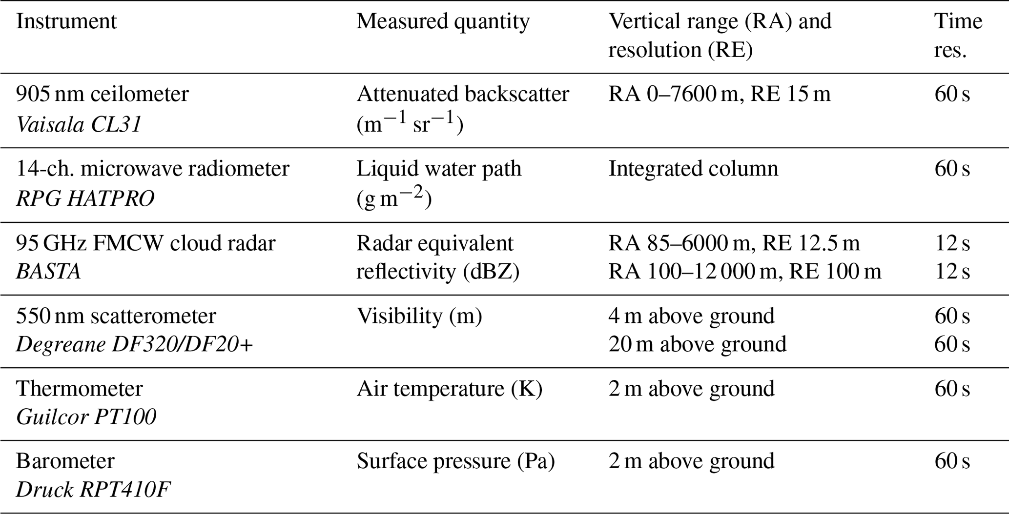
The SIRTA observatory is equipped with a large array of instruments, tailored for observing fog and fog processes (Haeffelin et al., 2010; Wærsted, 2018). A subset of these instruments is selected for studying the proposed conceptual model, based on the required inputs. These instruments are listed in Table 1.
Data from three remote-sensing instruments are used: a CL31 ceilometer, a BASTA cloud radar, and a HATPRO microwave radiometer. The CL31 is a widely used instrument for cloud base height (CBH) detection, with a vertical resolution of 15 m (Kotthaus et al., 2016). In this study it is used to retrieve the CBH of low stratus clouds preceding fog events and to track CBH lifting during temporary or definitive dissipation of the fog layer.
The cloud radar BASTA is a 95 GHz FMCW radar used to retrieve vertical profiles of cloud reflectivity, up to 12 km of height (Delanoë et al., 2016). It operates continuously alternating between 12.5, 25, and 100 m resolution modes every 12 s. The 12.5 m mode has the highest vertical resolution, and therefore it is used to retrieve fog CTH. Meanwhile, the 100 m mode is the most sensitive and reaches the highest altitude of 12 km and therefore is used to detect the presence of clouds above the fog layer.
The multi-wavelength microwave radiometer (MWR) HATPRO measures the integrated LWP of the atmospheric column. The manufacturer-specified uncertainty of the LWP product is ± 20 g m−2, but for a relatively small LWP (< 40 g m−2), investigations indicate that the uncertainty is within ± 5–10 g m−2, at least when the fog forms in clear sky so that a possible time-independent bias can be corrected for (Marke et al., 2016; Wærsted et al., 2017). When no other cloud is present above the fog layer, LWP measured by the MWR will correspond to fog LWP. Thus, MWR and cloud radar data can be combined to perform reliable fog LWP retrievals.
These remote-sensing instruments are complemented by a weather station 2 m above the surface and two scatterometers, at 4 and 20 m above the surface. The weather station provides the thermodynamic data necessary to calculate the saturated adiabatic lapse rate Γad(T,P), and the 4 m scatterometer provides the visibility data used to detect fog events and to calculate fog LWC at the surface. Visibility data are also used to complement the CL31 CBH estimation for very low cloud layers.
Table 1List of instruments and measurements used in this study (italics indicate the brand and model of the instrument).
3.2 Fog event detection
Fog periods are identified using a scheme based on previous work done by Tardif and Rasmussen (2007) and Wærsted et al. (2019). This method requires the re-sampling of the surface visibility time series to 5 min blocks. Each 5 min block is assigned a “fog” or “clear” value, depending on the distribution of visibility in its time period. A block is assigned the fog value when more than half of the visibility measurements are less than 1000 m, and it is assigned the clear value otherwise.
After assigning values to each block of the complete visibility time series, we analyze groups of five consecutive blocks in a sliding manner. These five contiguous blocks are defined as a construct, and its value is positive when the central and at least two others are fog blocks, and it is negative otherwise.
A fog event forms when a positive construct is encountered, with a formation time defined as the central time of the first fog block in the construct. Conversely, a fog event dissipates when the last positive construct is followed by either a negative construct or three consecutive clear blocks. Fog dissipation time is set as the central time of the block immediately after the last fog block in the last positive construct. Fog events separated by less than 1 h are merged, and all fog events lasting less than 1 h are discarded. This algorithm provides the formation and dissipation time of 217 fog events between July 2013 and March 2020. It is worth noting that this method, based on visibility measurements only, does not classify the fog type. Hence, all fog types are considered in this study.
3.3 Data processing
After identifying the fog events, it is necessary to process raw measurements from the instruments into information that can be used by the conceptual model. To study the conceptual model variables during fog events and the time period surrounding them, observational data are automatically processed and re-sampled to 5 min time blocks, covering the period from 3 h before fog formation to 3 h after fog dissipation.
CBH is retrieved using a threshold value of m−1 sr−1 on the CL31 attenuated backscatter measurements, following the method of Haeffelin et al. (2016). When the liquid layer is closer than 15 m to the ground, the CL31 cannot identify the CBH anymore, and therefore the scatterometer measurements are checked, setting the CBH as 0 m when visibility drops below 1000 m. Both CBH and visibility measurements are averaged to 5 min time blocks, matching the blocks used by the fog detection algorithm.
The cloud radar is used to retrieve fog CTH and to detect the presence of higher clouds above the fog layer, based on its vertical reflectivity profile (Wærsted et al., 2019). To retrieve CTH, reflectivity signals in each radar gate are analyzed, starting from the gate closest to the CBH and checking one gate at a time, going upwards. CTH is estimated as the height of the gate under the first gate where no cloud signal is detected. A gate is considered to have a valid cloud signal if more than half of the reflectivity samples in a 5 min time block are not removed by the automatic noise filtering algorithm of the radar (Delanoë et al., 2016). As with CBH, time blocks used in CTH retrievals match those defined for fog detection.
A limitation of this method is that the minimum detectable CTH is 85 m. Under this height, radar interference becomes very significant, making the differentiation between a valid cloud signal and noise very difficult. In this situation the CTH retrieval is not possible, and therefore the associated time block would not have a valid CTH value.
Radar data are also used to create a flag indicating the possible presence of liquid clouds above the fog layer when another valid signal is observed above fog CTH, within the first kilometer for the 12.5 m resolution mode or within the first 6000 m for the 100 m resolution mode. This flag is used in LWP retrievals, as explained below.
The HATPRO microwave radiometer performs LWP retrievals of fog every 60 s, which are then averaged and re-sampled to the 5 min time block grid. Additionally, when a given time block has an associated flag indicating the possible presence of higher liquid clouds, the LWP sample is declared not valid. This is done to ensure that the LWP samples are reliable, by avoiding a possible fog LWP overestimation when liquid clouds are present.
Time series of surface temperature and pressure are all averaged to match the 5 min time blocks. The saturated adiabatic lapse rate Γad(T,P) is calculated for each of these time blocks using these measurements and the equations in Appendix A.
In this scheme, it is important to note that to have a valid sample of conceptual model variables in a given 5 min time block, the block must have valid measurements of fog CTH, LWP, surface visibility, and surface temperature and pressure. Therefore, it is possible to have fog cases without valid samples of conceptual model variables for some time periods. We decided to use these cases (if they comply with the data quality control of Sect. 3.4) and to consider all the samples with valid conceptual model calculations for the statistical analyses.
3.4 Data quality control
After data treatment is complete for all automatically detected fog events, a manual check is done to remove cases where data are unreliable. This happens when instruments operate under non-optimal conditions or when the upper liquid cloud flagging algorithm did not work correctly.
This control consist of accepting or removing complete fog cases and their associated dataset. A fog case is removed from the data pool if measurements taken when the fog takes place comply with at least one of the following criteria:
-
Data are taken during or after strong precipitation: strong precipitation wets the microwave radiometer radome, leading to unreliable LWP retrievals for an unpredictable period of time that can last up to hours, even when following all maintenance instructions (Görsdorf et al., 2020). Additionally, strong rain leads to difficulties in identifying the fog CTH because the strong reflectivity from rain hides the weaker returns from suspended fog droplets.
-
There are no valid data blocks: no CTH or LWP retrievals could be made for the given fog event. This can happen when fog is thinner than 85 m or when liquid clouds are present above fog for the complete event duration.
-
Fog and cloud borders are not well identified: in some cases the automatic cloud border detection algorithm fails, leading to unfiltered LWP retrievals with liquid clouds above or to a bad estimation of fog CTH when upper clouds are too close to the fog layer. The latter can be seen in the radar data as multilayer fog formed by the union of two previously independent cloud layers. This situation departs from the single well-mixed layer assumption, and therefore the conceptual model is not applicable.
The quick looks for the accepted and rejected fog cases are available in the article Supplement. After this stage we end with 80 valid fog cases and 137 rejected cases, where 50 were removed because of criterion 1, 69 because of criterion 2, and 18 because of criterion 3. These 80 valid fog cases have at least one valid sample of conceptual model variables (see Sect. 3.3), which are then used in the next stages of data analysis and results.
4.1 Fog adiabaticity
A key parameter in the calculation of the CLWP is the equivalent fog adiabaticity αeq (Eq. 4). This parameter has been previously studied in the literature for boundary layer stratocumulus and stratus clouds, where typically observed values of αeq range between 0.6 and 0.9 (Slingo et al., 1982; Boers et al., 1990; Boers and Mitchell, 1994; Braun et al., 2018). In this situation, clouds have an adiabatic profile and are buoyant (Betts, 1982). Buoyancy is important because it is necessary to have dissipation by lifting of the fog base.
Hence, it is interesting to study whether these adiabaticity values also apply to fog, which is a special cloud case with a solid lower boundary at the surface. Therefore, we use the complete database to calculate αeq by closure, with Eq. (6). This equation is an inversion of the conceptual model formulation of Eq. (3c) and enables an estimation of the adiabaticity while correcting the impact of the LWC accumulation at the fog base. We only perform αeq retrievals when visibility is below 2000 m, in order to remain close to fog conditions.
Figure 3a shows the resulting equivalent adiabaticity versus CTH and LWP. The results indicate that increases for greater values of LWP and CTH. In addition, negative adiabaticity values are found for lower LWP values, especially below 30 g m−2.
To study this behavior in more detail, Fig. 3b shows a boxplot with the statistics of for different LWP ranges. Here we observe that negative adiabaticity values become frequent when the LWP is below the 30–40 g m−2 range, until occurring for more than half of the samples when the LWP is below 20 g m−2.
This can be explained by considering that fog with an LWP of less than ∼ 30 g m−2 is not optically thick (Wærsted et al., 2017). Under this condition, the liquid water condensation happens everywhere in the liquid layer, but it is mostly driven by surface cooling. This process is associated with stable atmospheric conditions, where vertical mixing is almost negligible (Zhou and Ferrier, 2008). Under this regime, the LWC will be distributed according to the cooling and condensation rate at each height, and therefore it is possible to have situations where surface LWC is greater than LWC values above, especially during radiation fog formation. This situation would lead to the observed negative αeq values.
When fog LWP surpasses the 30–40 g m−2 range, its adiabaticity converges to ∼ 0.7, which, as stated in the previous lines, is a value consistent with typical observations of boundary layer stratocumulus (Slingo et al., 1982; Boers et al., 1990; Boers and Mitchell, 1994; Cermak and Bendix, 2011; Braun et al., 2018). This can be explained because fog gradually becomes opaque to infrared radiation when its LWP surpasses ∼ 30 g m−2 (Wærsted et al., 2017). In this scenario, LWC generation is mostly driven by radiative cooling at the fog top. This radiative cooling induces a temperature gradient between the fog top and the surface, leading to convective motions. An increase in the intensity of convection will be correlated with an increase in fog CTH because the additional energy would enhance boundary layer development. Then, as fog becomes deeper, it is expected that the relatively stronger convective motions associated would drive the vertical liquid water mixing closer to what is observed in boundary layer clouds. This result and theory also indicate that dissipation by base lifting should happen when the LWP is at or above the 30–40 g m−2 range, when the layer is adiabatic and buoyant.
Finally, we can also observe that adiabaticity sometimes reaches values slightly greater than 1, which can be associated with periods when fog is superadiabatic. This is possibly caused by an excess of liquid water with respect to the extent of the fog column, which may be caused by the surface presence, as introduced in Sect. 2.
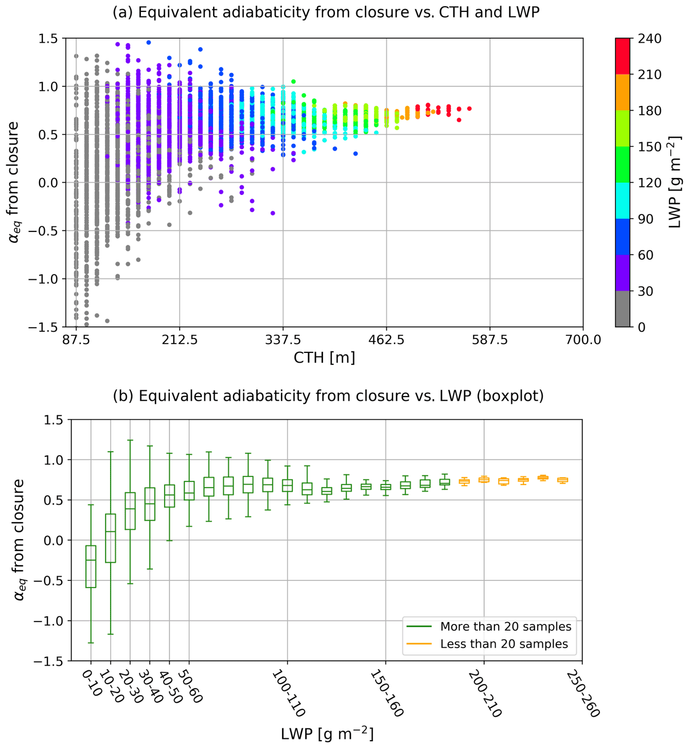
Figure 3(a) Equivalent adiabaticity versus fog CTH and LWP. The equivalent adiabaticity is calculated by closure, using Eq. (6). (b) Boxplot of the equivalent adiabaticity, calculated by closure, for different LWP ranges. In both figures only samples with visibility below 2000 m are considered.
4.2 Adiabaticity parametrization as a function of CTH
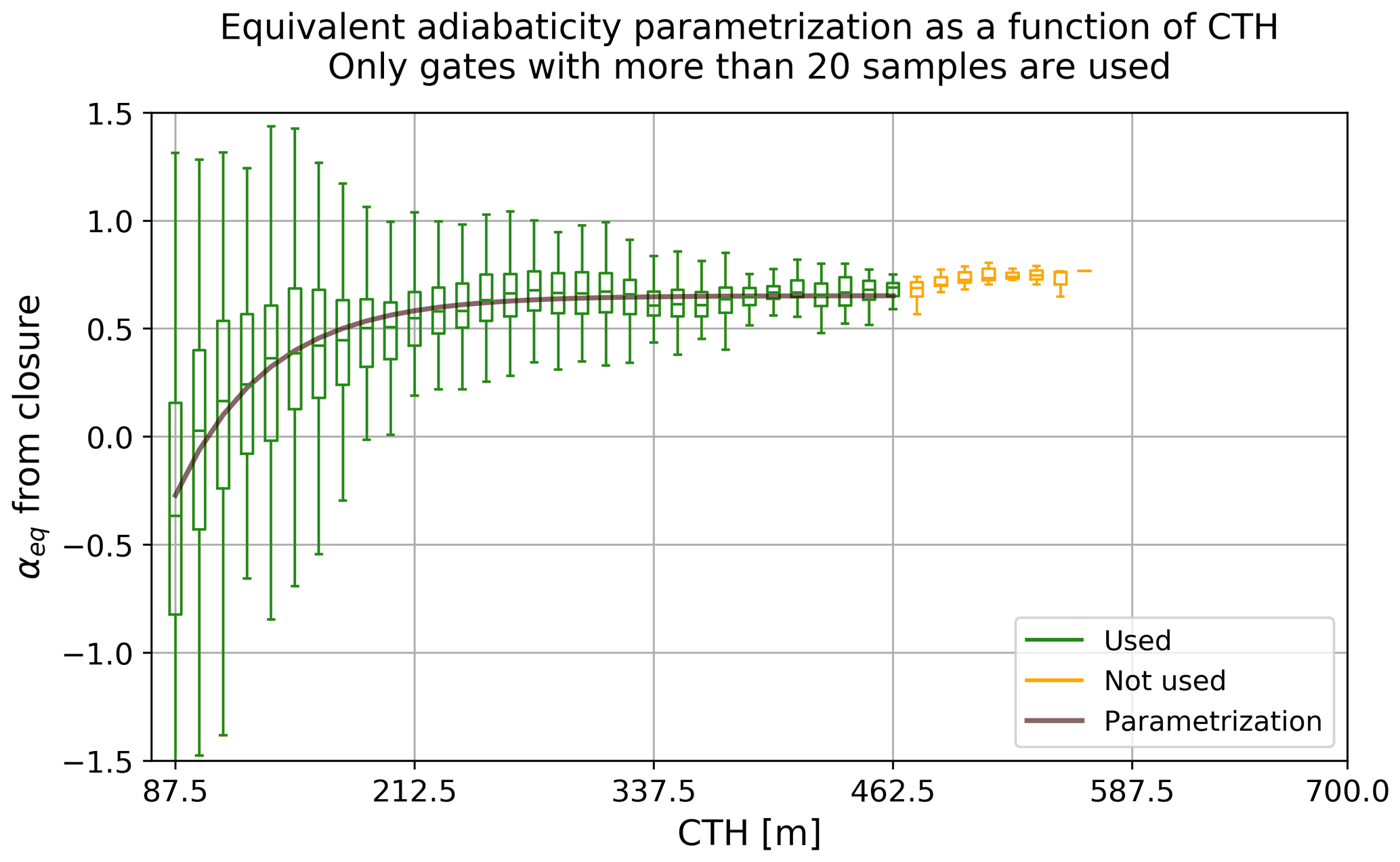
The strong correlation between adiabaticity and CTH observed in Fig. 3a suggests that αeq can be parametrized as a function of CTH. The parametrization curve is calculated by minimizing the error of the model presented in Eq. (7) with respect to the median αeq value at each radar range bin (see Fig. 4). To reduce uncertainty due to lack of data, only bins with more than 20 valid samples are used.
The retrieved values for each coefficient are α0=0.65, H0=104.3 m, and L=48.3 m. These parameters come from fog statistical behavior and can be interpreted as follows: α0 is the equivalent adiabaticity value that fog reaches when it has completely transitioned into an adiabatic regime. H0 is the usual height at which LWC starts to increase with height. Based on adiabaticity, L indicates that the transition from stable to adiabatic fog is possible when CTH reaches 150 m and very likely when CTH is above 250 m (H0+L and H0+3L, respectively).
In principle, the adiabaticity parametrization is valid for CTH values below 462.5 m, where the parametrization is derived. Beyond this height there are not enough data to guarantee its reliability; however, it is likely that adiabaticity should remain close to the convergence value of 0.66 based on our observations and on what has been previously published in the literature (Slingo et al., 1982; Boers et al., 1990; Boers and Mitchell, 1994; Cermak and Bendix, 2011; Braun et al., 2018).
4.3 Conceptual model validation
In this section we study fog statistical data to study how they behave with respect to the conceptual model. Figure 5a shows all CTH, LWP, and surface LWC measurements taken when fog is present (visibility less than 1000 m). Data are separated into different temperature ranges. Modeled LWP and CLWP curves are shown. LWP and CLWP theoretical curves are calculated using Eqs. (3c) and (4), respectively, with the αeq(CTH) parametrization derived in Sect. 4.2. Each hexagon color is given by the mean LWC0, calculated using all the data in their respective CTH + LWP space. Hexagons with less than five samples within their surface are removed, since they are likely to be associated with non-replicable, noisy data.
This figure shows good agreement between the theoretical curves and observed results. Most LWP samples are higher than the critical value, as the model predicts when visibility is less than 1000 m. Additionally, it can be seen that for a fixed CTH, LWP increases with LWC0. This behavior seems to be well captured in the current conceptual model formulation, as the difference between the three lines shows (each theoretical LWP line has a different LWC0 value, indicated in the legend).
Figure 5b shows data samples taken when visibility is between 1000 and 2000 m, as a scatterplot. As in Sect. 4.1, the 2000 m superior limit to visibility is selected, to remain close to fog conditions where the conceptual model is valid. LWP of these data samples should be less than the CLWP line for these visibility values; however, we observe that sometimes they can also be larger. This can be explained by two main factors: CLWP is calculated for a single temperature, while data temperature varies within a range, and there are instrumental uncertainties. HATPRO LWP uncertainty is around 10 g m−2, while radar CTH retrieval has a resolution of 12.5 m. This uncertainty is present in this retrieved data and is also likely to be propagated inside the αeq(CTH) parametrization, introducing some variability in the results. However this is not deemed critical, since variability around the CLWP line is smaller than 10 g m−2 and because the fog life cycle studies of Sect. 5) verifies that the LWP is lower than the critical value before fog formation and after fog dissipation.
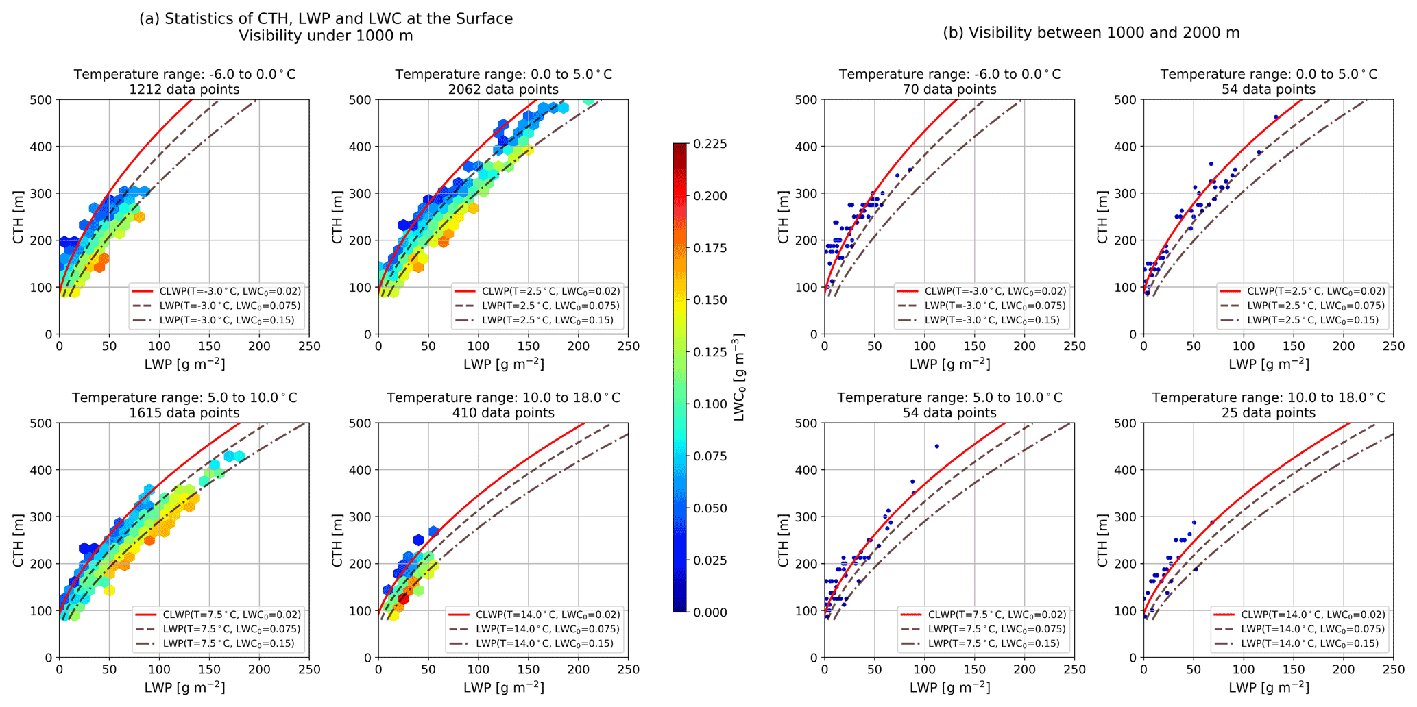
Figure 5Observations of CTH, LWP, and LWC at the surface for different temperature and visibility ranges. Data associated with visibility values below 1000 m are on the left (a), while data measured with visibility values between 1000 and 2000 m are on the right (b). Conceptual model theoretical LWP and CLWP lines for different conditions, indicated in the legend, are superimposed. The adiabaticity values used in the conceptual model calculation are calculated using the adiabaticity parametrization of Sect. 4.2.
Finally, we perform an evaluation of how well the conceptual model predicts fog LWP, based on CTH, temperature, pressure, and surface LWC inputs. These variables are used to calculate the conceptual model LWP with Eq. (3c), with the αeq(CTH) parametrization of Sect. 4.2 and compared against HATPRO LWP retrievals. Results are shown in Fig. 6. Here we can see that most samples are close to the 1 : 1 line for LWP values less than approximately 190 g m−2. Beyond this LWP value some deviation appears; however, there are not enough data available to verify if this is a systematic error in the model or in how data were taken. Despite this deviation, the good agreement between modeled and observed LWP can be seen in the linear fit, with a slope equal to 1, and in the RMSE of just 10.5 g m−2, which is very close to the LWP retrieval uncertainty.
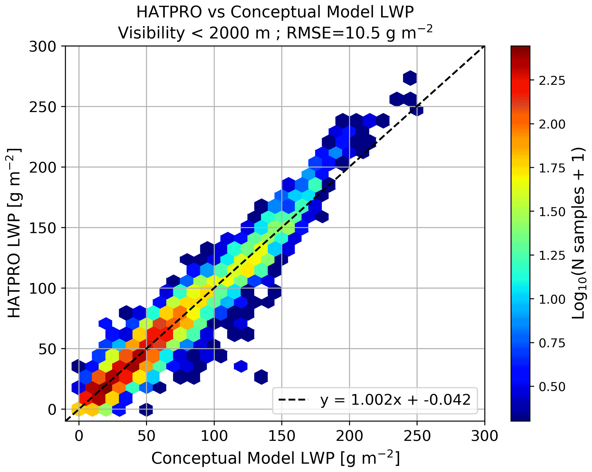
Figure 6Two-dimensional histogram comparing HATPRO and conceptual model LWP values, for data retrieved when visibility is less than 2000 m. Conceptual model LWP is calculated using fog CTH, fog LWC at the surface derived from visibility, surface temperature, surface pressure, and the adiabaticity parametrization of Eq. (7). Under these conditions, the conceptual model predicts LWP with an RMSE of 10.5 g m−2 and an almost perfect linear relationship.
4.4 Drivers of RLWP temporal variations
Equation (5) indicates that changes in both LWP and CTH can contribute to RLWP depletion and therefore to fog dissipation. To quantify the relative impact of LWP and CTH changes in RLWP, we calculate the time derivative of Eq. (5). By assuming constant temperature and pressure and using the α(CTH) parametrization of Sect. 4.2, we obtain Eq. (8).
This equation shows that RLWP changes are proportional to LWP variations and to CTH variations weighted by the function . This function, written explicitly in Eqs. (9a) and (9b), converts CTH variations into units of grams per square meter and thus enables a comparison between both effects.
Equation (8) implies that RLWP depletion, and thus fog dissipation, can occur by LWP reduction and/or by CTH growth. It also indicates that it is possible to have compensating effects enhancing fog persistence; for example, fog that is reducing its LWP could persist if its CTH is also decreasing (which can happen under strong subsidence). Another implication is that it is possible to have fog dissipation even if LWP is increasing quickly, through a fast increase in CTH. The case studies of Sect. 5.1 show how useful this separation between LWP and CTH effects can be, by analyzing some examples of the previously mentioned scenarios. Section 5.2.3 shows statistical results of fog RLWP, LWP, and CTH time derivatives just before dissipation.
5.1 Case studies
We present three case studies to illustrate the behavior and role of changes in LWP and CTH in the presence of fog at the surface during the fog life cycle (Figs. 7, 8, and 9). For each case we provide a five-panel figure that illustrates the time series of fog–stratus layer boundaries, reflectivity profile, 4 and 20 m horizontal visibilities, the fog–stratus layer measured LWP and computed RLWP, temperature and closure adiabaticity, and the change rate of RLWP, with the individual contributions from LWP and CTH variations.
In all three cases, we observe that fog is present at the ground (4 m height visibility < 1 km) when the RLWP is greater than 0 g m−2. RLWP changes at a rate of ± 10 g m−2 h−1, with values reaching ± 30 g m−2 h−1 at times. The LWP estimation of all case studies is done directly using the HATPRO, verifying that the radar does not detect signals from liquid clouds below 6 km of height.
Case study 1 (Fig. 7). Radiative fog occurring during fall season (31 October 2015) that forms 6 h before sunrise and dissipates about 3 h after sunrise at 10:25 UTC. The fog layer is about 200 m thick during the entire fog life cycle with a water content of 30–60 g m−2. This LWP range and the adiabaticity values close to 0.6 indicate that fog is optically thick and can be regarded as a well-mixed layer for most of its duration. The RLWP is not large, mostly near +10 g m−2, with a maximum value of 30 g m−2 observed 2–3 h before sunrise. CTH changes are relatively slow during the entire fog life cycle, with values less than 50 m h−1. From 03:00 to 05:00 UTC, the CTH increases, which acts as RLWP depletion of nearly −20 g m−2 h−1, while at the same time the LWP increases with a rate reaching +50 g m−2 h−1 resulting in a net increase in RLWP. After 05:00 UTC, the trends in CTH and LWP reverse. The CTH subsides slowly (about −20 m h−1) contributing positively to the RLWP at a rate of nearly +5–10 g m−2 h−1, while the LWP initiates a progressive and nearly monotonous decrease of −10 g m−2 h−1 that brings the RLWP to 0 g m−2 at 09:00 UTC. The progressive drying of the fog layer is also identifiable in the closure adiabaticity value, which starts to decrease just after sunrise. After 09:00 UTC, the near-surface visibility initiates a rapid increase, exceeding 1 km at 10:25 UTC, a time at which the entire fog layer is dissipated. The complete layer dissipation and the increasing temperature makes it highly unlikely that fog will re-form in the coming hours. Note on Fig. 7f that LWP and CTH contributions to RLWP are nearly always of opposite signs but not equal in magnitude.
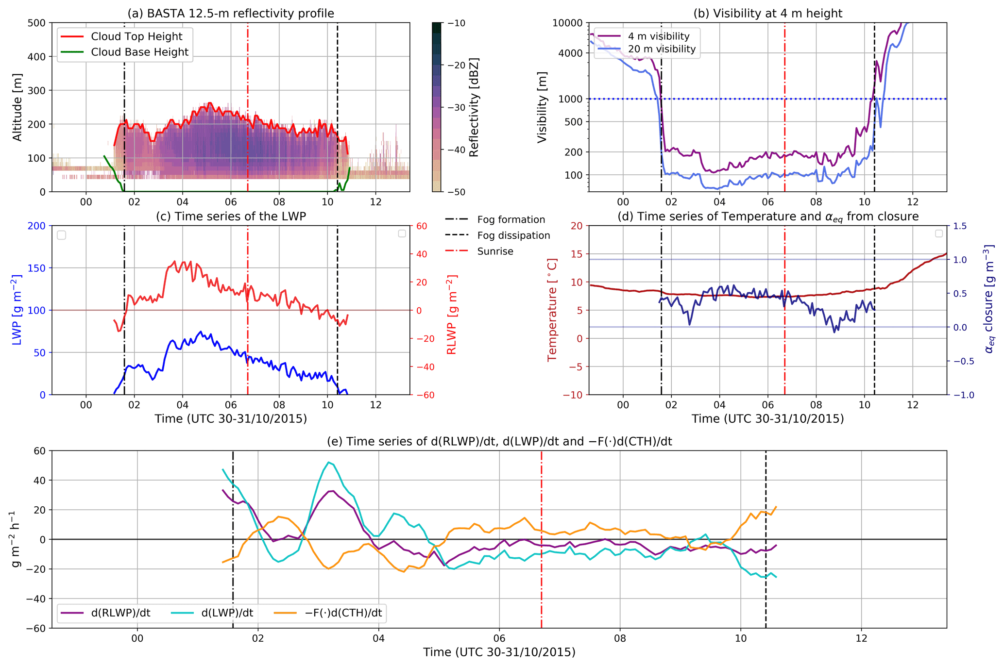
Figure 7Case study 1. (a) Cloud base height (CBH), cloud top height (CTH), and the cloud radar 12.5 m resolution reflectivity profile for the first 1000 m of height. (b) Horizontal visibilities at 4 and 20 m of height. (c) Fog–stratus layer measured LWP and computed RLWP. (d) Temperature and closure adiabaticity (calculated only when visibility is less than 2000 m). (e) Change rate of RLWP, with the individual contributions from LWP and CTH variations. In each panel, the time of fog formation and fog dissipation are clearly marked as is the time of sunrise.
Case study 2 (Fig. 8). Another radiative fog that occurs in the fall season, just a few days apart from case study 1 (26 October 2015). It forms just 3 h before sunrise and dissipates about 3.5 h after sunrise at 10:55 UTC. The fog layer is about 200 m thick during the mature phase of the fog life cycle and nearly doubles between sunrise and the time of dissipation, while the water content remains above 50 g m−2. After fog formation, RLWP reaches 30 g m−2 in about 1 h and remains at this level for about 2 h. Fog adiabaticity indicates that after the first hour from formation fog remains in a well-mixed state. Around sunrise, RLWP initiates a nearly monotonous decreasing trend of −10 g m−2 h−1 that will last until fog dissipation. The negative RLWP rate is driven by the rise in CTH that contributes negatively on RLWP with a rate that exceeds −20 g m−2 h−1, only partially compensated for by +20 g m−2 h−1 LWP increase rates. Oscillations in LWP and CTH contributions to RLWP are clearly visible in Fig. 8f. When there is strong cooling at the fog layer top, LWP and vertical circulation increase. This in turn increases the mixing with the layer above fog, resulting in a CTH increase. By contrast, processes associated with CTH subsidence tend to decrease LWP rates (Wærsted, 2018). In this case study, the depletion of RLWP is clearly driven by the CTH increase, and the fog LWP still exceeds 75 g m−2 at the time of dissipation.
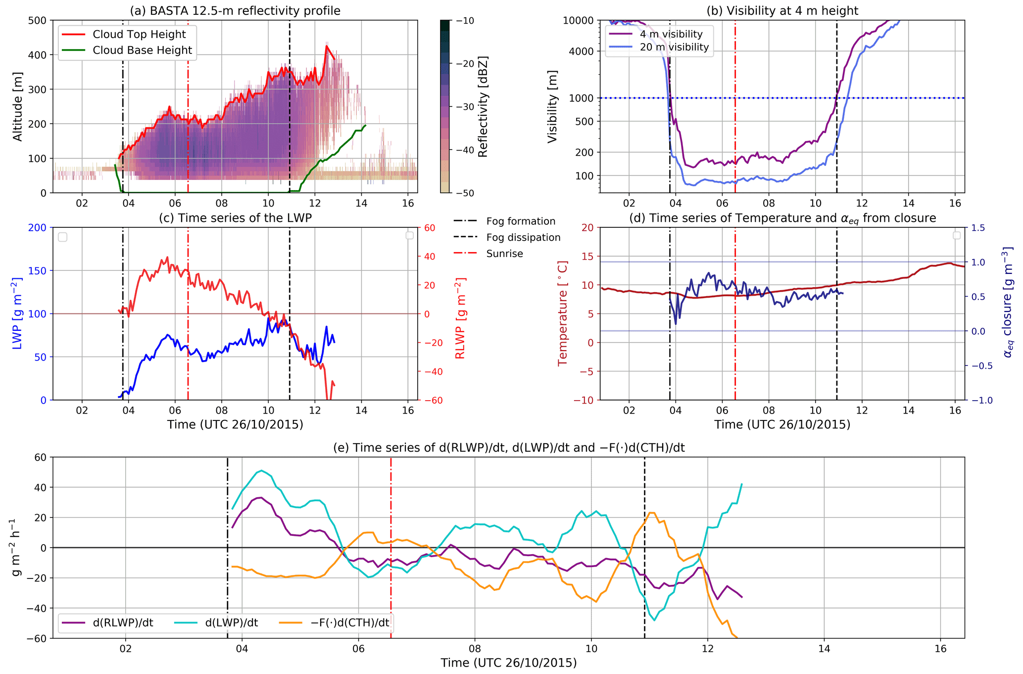
Figure 8Case study 2. (a) Cloud base height (CBH), cloud top height (CTH), and the cloud radar 12.5 m resolution reflectivity profile for the first 1000 m of height. (b) Horizontal visibilities at 4 and 20 m. (c) Fog–stratus layer measured LWP and computed RLWP. (d) Temperature and closure adiabaticity (calculated only when visibility is less than 2000 m). (e) Change rate of RLWP, with the individual contributions from LWP and CTH variations. In each panel, the time of fog formation and fog dissipation are clearly marked as is the time of sunrise.
Case study 3 (Fig. 9). Here we have a typical case of a very low stratus cloud layer with CTH near 250 m a.g.l. and an LWP that ranges from 25 to 50 g m−2. This combination leads to a negative RLWP that is insufficient for the stratus to deepen all the way to the surface. As expected for low stratus clouds, the value of closure adiabaticity is close to 0.6 for all valid samples (when visibility is less than 2000 m, to have valid conceptual model conditions with positive LWC at the surface). The stratus is present from 18:00 UTC onwards during 12 h with a near-surface visibility of about 2–3 km. From 18:00 until 23:00 UTC, RLWP is clearly negative, changing frequently from negative to positive rates of change (about ± 5 g m−2 h−1) as the contributions of LWP and CTH changes oscillate from positive to negative values (as also seen in Case 3). At 01:00 UTC, the stratus reaches a new equilibrium with an LWP hovering around 50 g m−2, which brings the RLWP very close to 0 g m−2. The fog CBH is then below 20 m a.g.l., as evidenced by the visibility values measured at 20 m a.g.l. (Fig. 9c). Between 04:30 and 06:30 UTC, the RLWP again becomes negative and the stratus base lifts. A strong increase in LWP (+40 g m−2 h−1) starting after 06:00 UTC leads to a positive RLWP after 06:30 UTC and the stratus layers deepen all the way to the surface. The trend in LWP reverses around 08:00 UTC (−20 g m−2 h−1), while the CTH remains mostly constant, hence reducing the RLWP towards 0 g m−2 before 10:00 UTC. This case study shows that the RLWP is also a good indicator of the possibility for a very low stratus layer to deepen into fog and then reversely for the fog to lift into a low stratus.
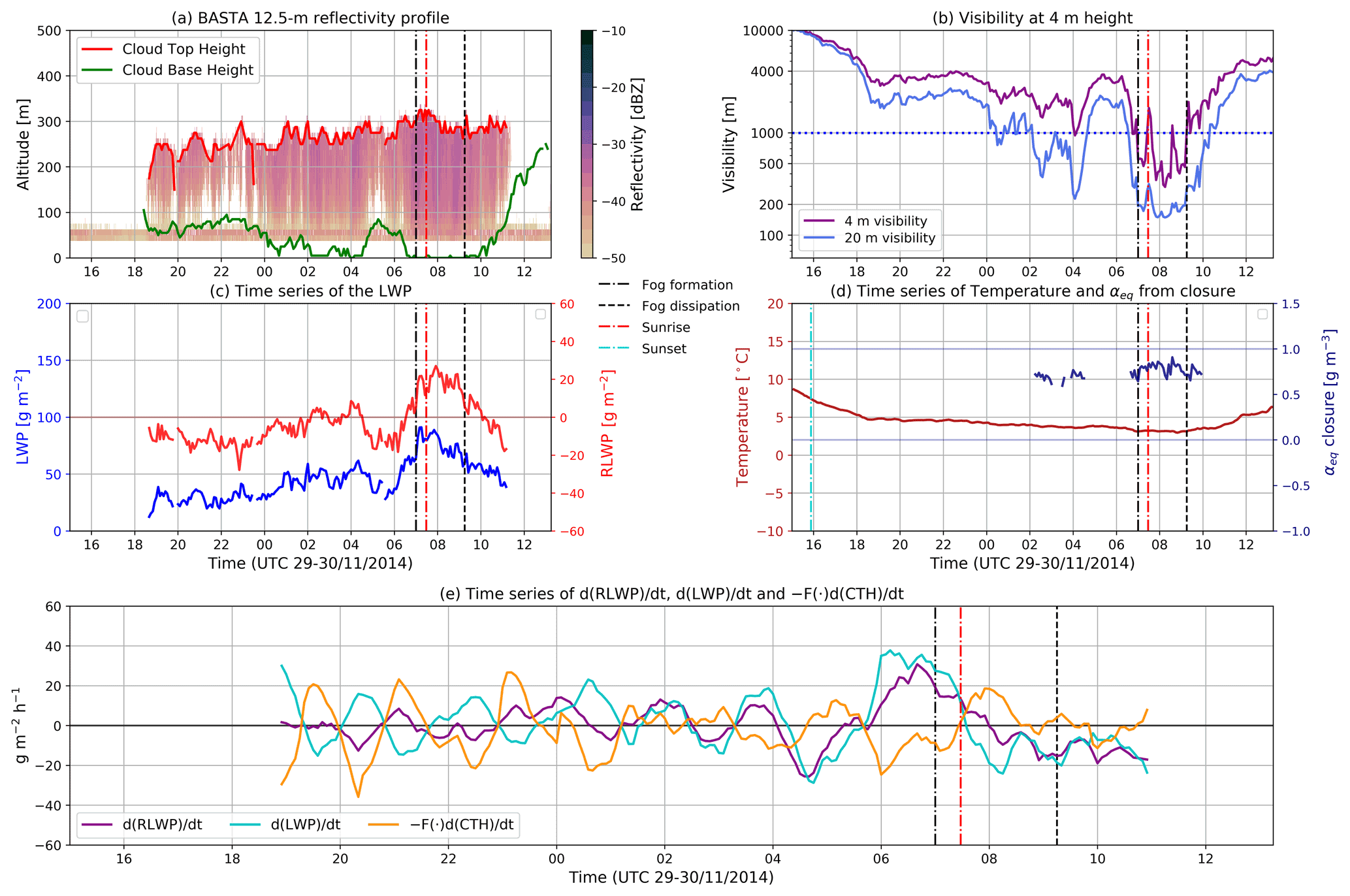
Figure 9Case study 3. (a) Cloud base height (CBH), cloud top height (CTH), and the cloud radar 12.5 m resolution reflectivity profile for the first 1000 m of height. (b) Horizontal visibilities at 4 and 20 m. (c) Fog–stratus layer measured LWP and computed RLWP. (d) Temperature and closure adiabaticity (calculated only when visibility is less than 2000 m). (e) Change rate of RLWP, with the individual contributions from LWP and CTH variations. In each panel, the time of fog formation and fog dissipation are clearly marked as is the time of sunrise.
5.2 Fog life cycle statistics
Taking advantage of our large database, we study the behavior of fog RLWP and its time derivative statistically, for three different periods: fog formation, mature stage, and dissipation. The objective is to identify patterns that these fog variables follow at each stage. This could lead to the development of new indicators to enhance the capabilities of fog forecasting models.
Fog formation statistics are taken between 90 min before and 90 min after the time block when fog formation is identified from visibility measurements (Sect. 3.2). Likewise, for the dissipation period the analyzed data are taken from 90 min before to 90 min after the dissipation time block. All remaining blocks between 90 min after fog formation and 90 min before fog dissipation are considered to be fog middle life data. Because of how the fog stages are defined, the cases included in this statistical analysis must have a duration of at least 3 h. This is valid for 56 cases, which are used for statistical analysis in the following sections.
The time derivative of the RLWP (and the sliding mean used in Fig. 10b.2) is estimated by calculating the slope of a linear fit on RLWP data within ±30 min of a given time block. The retrieved slope value is declared valid only if at least 75 % of the RLWP samples used in its calculation are valid.
5.2.1 Fog formation
Figure 10a.1 shows the statistical behavior of RLWP between 90 min before and 90 min after formation. It can be seen that at fog formation there is a transition from negative to positive RLWP values. The relatively lower amount of samples earlier than 35 min before fog formation happens because there are fewer fog cases were the cloud has formed that early or that have an identifiable CTH above 85 m. Yet, we can see that RLWP cannot be significantly lower than −10 g m−2 if fog forms within 30 min.
Additionally, in Fig. 10a.2 we can see that becomes positive about 1 h before formation and remains consistently positive for another hour after formation. This first hour after fog formation is when the fog reservoir grows the most, reaching a change rate of 10 to 25 g m−2 h−1, and it may be critical in establishing fog persistence for the coming hours. After this first hour, fog RLWP stabilizes around 10 to 20 g m−2 and the increase per hour is reduced until entering the mature stage.
All 56 fog cases lasting more than 3 h are considered for the statistics. However, since radiation fog is formed from a shallow layer close to the surface, these cases usually do not provide valid data points because their CTH cannot be retrieved with the radar (it can only observe CTH values above 85 m). Therefore, most of the data points before and around formation time are contributed by stratus-lowering fog events.
5.2.2 Fog mature stage
A histogram with RLWP values is shown in Fig. 10b.1. We can see that approximately 90 % of the time fog has a positive RLWP value, with a median value of 20.1 g m−2 and reaching up to ∼60 g m−2. Negative RLWP values in the fog mature stage are explained by short-term temporary lifting of fog from the surface, most likely caused by RLWP oscillations.
Figure 10b.2 shows the statistics of versus the sliding mean value of RLWP. This figure shows that RLWP and its time derivative are not correlated and that most of the time remains within ±20 g m−2 h−1. The very low median value of g m−2 h−1 shows that fog does not have a clear tendency of RLWP increase or decrease in the long term. Thus, during this stage of the fog life cycle, RLWP remains positive most of the time, with variations driven by oscillations in the value of .
The statistics for this period defined as the fog mature stage are derived using the 56 fog events lasting more than 3 h. In the fog mature stage several radiation fog cases will be developed beyond 85 m of CTH, and therefore both stratus lowering and radiation fog cases contribute to the statistics.
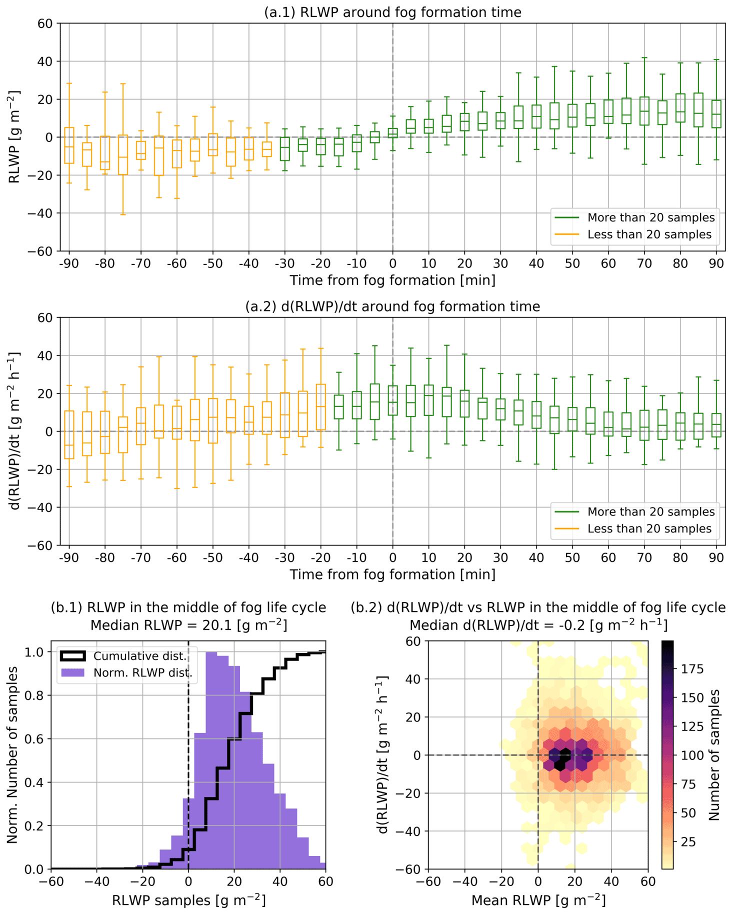
Figure 10The boxplots of (a.1) and (a.2) represent RLWP and statistics for each time block 90 min before and after fog formation. The boxplot shows the 25th, 50th, and 75th percentiles and the maximum and minimum values. The number of samples per bin is shown in Fig. S2 of the Supplement. Panels (b.1) and (b.2) show RLWP and statistics during fog middle life, between 90 min after fog formation and 90 min before dissipation, calculated using 4064 and 3952 samples, respectively. The ordinate axis of (b.1) is associated with the cumulative and normalized distributions.
5.2.3 Fog dissipation
In the latter stage of the fog life cycle, shown in Fig. 11a.1, RLWP decreases consistently from positive values associated with the middle of the life cycle until reaching negative values after fog dissipation. Additionally, there are almost no RLWP samples above ∼30 g m−2 observed in the last 30 min before dissipation. Hence, an RLWP value above ∼30 g m−2 may be interpreted as an indicator of fog persistence.
Figure 11a.2 shows that the monotonous decrease in RLWP begins about 60 min before fog dissipation and can commonly reach values of about −10 to −30 g m−2 h−1. These negative values in the time derivative continue after fog dissipation and can be explained by further lifting or drying of the remaining low stratus cloud (Wærsted et al., 2019).
To study what the main driver of fog dissipation is, Fig. 11b shows the calculated , , and trends, defined in Sect. 4.4, using the last 60 min of data before dissipation. Theoretically, dissipation can only happen when the RLWP decreases, which only happens when the sum of the LWP and CTH time derivative terms is negative (Eq. 8). This matches the results of Fig. 11, which has most points in the quadrants leading to the aforementioned condition. The few points that show an RLWP increase before dissipation, to the right of the dashed line, are associated with uncertain retrievals due to low absolute RLWP values or fast RLWP depletion in the few minutes just before dissipation (time trends are calculated using 1 h linear fits). Additionally, observations confirm that fog dissipates under the same scenarios predicted in Sect. 4.4. Here the conceptual model predicts that fog could dissipate, even when the LWP is increasing, if the RLWP reduction from layer thickening is larger (strong CTH increase). Conversely, fog can also dissipate when the LWP decreases, even when the CTH subsides. Finally, some cases dissipate with the contribution of both effects: LWP decrease and layer thickening.
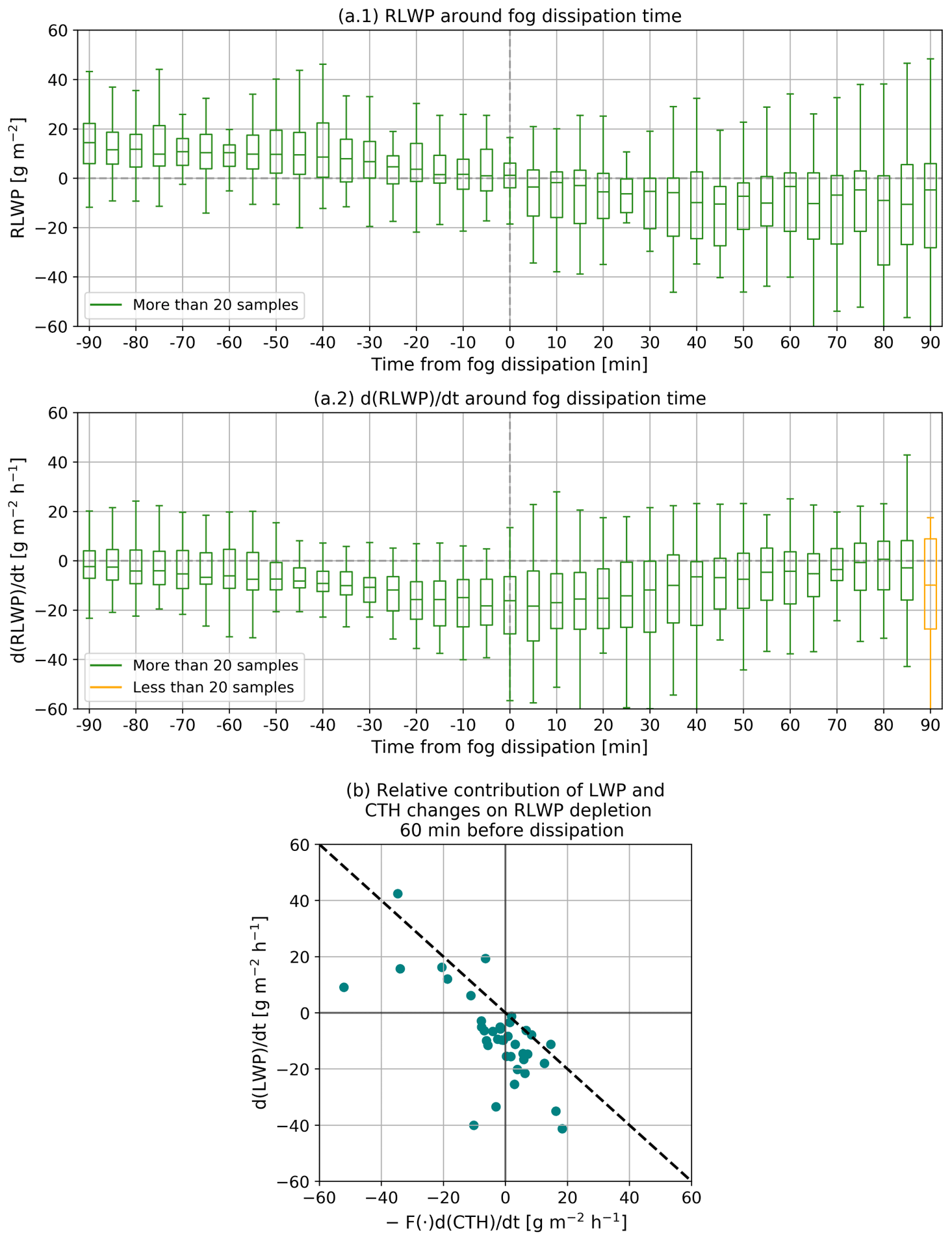
Figure 11The boxplots of (a.1) and (a.2) show RLWP and statistics for each time block, 90 min before and after fog dissipation. These statistics are derived using 56 fog events; however, there may be less than this amount of valid samples for each bin. The number of valid samples per bin is shown in Fig. S3 of the Supplement. Panel (b) shows the impact of LWP and CTH variations in RLWP depletion, using data from the last 60 min before dissipation. The dashed line indicates the theoretical limit where fog dissipation is possible (only to the left of this line). In quadrants II and III cloud base lifting contributes to RLWP decrease, while in quadrants III and IV the LWP decrease contributes to RLWP depletion. This panel contains 40 valid samples from 56 fog cases, calculated using the method explained at the beginning of Sect. 5.2.
This work presents a conceptual model for adiabatic fog that relates fog liquid water path to its thickness, surface liquid water content, and adiabaticity. The model predicts that LWP can be split into two contributions: the first is proportional to the adiabaticity and the square of CTH and the second is the product of surface LWC and CTH. The latter dependency is due to an excessive accumulation of water with respect to an equally thick cloud, which appears in fog because the surface presence limits vertical development.
This excess accumulation of water motivates the definition of two diagnostic parameters, which later will prove to be key in understanding fog evolution: the critical LWP and the reservoir LWP. The critical LWP (CLWP) is the minimum amount of column water that would fill the fog layer and cause a visibility reduction down to 1000 m at the surface. The critical LWP can be calculated using the conceptual model, by imposing a surface LWC equivalent to 1000 m visibility. Meanwhile, the reservoir LWP (RLWP) is the difference between fog LWP and the critical value and represents the excess of water that enables fog persistence. Case studies and statistical results show that the reservoir LWP is positive when fog is present and reaches 0 g m−2 at about the same time as fog dissipation.
The model is used to statistically study fog adiabaticity. Important conclusions are that thinner fog, with an LWP of less than 20 g m−2, has adiabaticity values below 0.6 and can even reach negative values. This happens when the fog layer is not yet opaque during the fog formation stage, when LWC distribution is not even and may be larger closer to the surface. In this situation fog is not buoyant, and therefore it may not lift when the RLWP reaches 0 g m−2. Conversely, when fog is developed, its adiabaticity value gets closer to previously observed values for boundary layer fog, converging at approximately 0.66 for fog with an LWP greater than ∼ 30–40 g m−2. Here the fog layer is adiabatic, and therefore the fog base should lift when the RLWP depletes down to 0 g m−2. Adiabaticity results are highly variable for LWP values between 20–30 g m−2, and therefore it may be necessary to include additional observations to discern the adiabaticity of the fog layer in this LWP range.
Another result from the study of adiabaticity is an adiabaticity parametrization as a function of fog thickness, which can be used to estimate fog LWP and to perform conceptual model calculations. The estimation of fog LWP has an RMSE of 10.5 g m−2, which is close to the uncertainty in LWP measurement of 10 g m−2, validating the modeled dependency of the LWP on surface LWC, temperature, pressure, and CTH.
The temporal derivative of the RLWP is studied, obtaining an analytic formulation that enables the quantification of the contribution of LWP and CTH variations to the depletion of the reservoir and therefore leading to fog dissipation. This formulation, which is validated by observations, indicates that fog dissipation will depend on the ratio between LWP and CTH variations and that fog can dissipate by lifting as long as the net RLWP trend is negative, even if (1) LWP and CTH are both increasing, (2) LWP is decreasing and CTH increasing, and (3) LWP and CTH are both decreasing.
Statistical observations of the fog life cycle indicate that the RLWP increases, in general, about 60 min before and after fog formation. This is followed by positive RLWP values, during fog middle life, that may oscillate or vary depending on the LWP and CTH evolution. Then, about 60 min before dissipation, the RLWP starts to decrease consistently until reaching 0 g m−2 at dissipation time.
The aforementioned conclusions and the paper results indicate that the RLWP and its time derivative can be used as indicators of the fog life cycle stage, at the local scale. This enables its potential use as an additional diagnostic variable, to quantify how close fog is from dissipation. This may complement visibility measurements at key sites affected by fog, such as airports and land roads, and help improve their logistics to reduce costs and the probability of accidents (Tardif and Rasmussen, 2007).
At present, the RLWP provides an estimation, in real time, of the excess of water of fog that enables the fog layer to remain at the surface. This can already be used as a diagnostic to estimate how likely fog persistence is for the coming minutes, based on the instant RLWP value and its trend (fog dissipation nowcasting). For example, results indicate that fog will not dissipate in the next 30 min if its RLWP is greater than ∼ 30 g m−2. Additionally, the RLWP must have a decreasing trend before dissipation, and therefore a positive trend would indicate fog persistence. This result could be improved by introducing forecasting tools to the conceptual model scheme. Forecasting when the RLWP will become 0 g m−2 would provide a proxy to predict fog dissipation by base lifting. This forecasting could be done, for example, by considering physical processes. They provide information on fog evolution and could be used to estimate how the LWP and CTH, and thus the RLWP, will evolve in the near future (e.g., Wærsted et al., 2019).
Another interesting perspective would be to test conceptual model calculations using the output of fog large-eddy simulations (LES). If the conceptual model variables behave as theoretically expected in these simulations, they could be used to further study the impact of microphysics or surface properties on fog adiabaticity.
Another area of interest would be to study the conceptual model at other sites with frequent fog events. When fog is adiabatic (LWP > 30–40 g m−2), the observed equivalent adiabaticity results are consistent with values observed at other sites. This suggests that the conceptual model could be applicable at other sites with similar fog types (continental midlatitude fogs), with possible variations in the adiabaticity parametrization due to local conditions. This remains to be verified using real observations.
It would also be of interest to study how the direct retrieval of adiabaticity profiles from cloud radar reflectivity profiles could be used to improve the accuracy of the RLWP estimation, compared to the use of a single equivalent value.
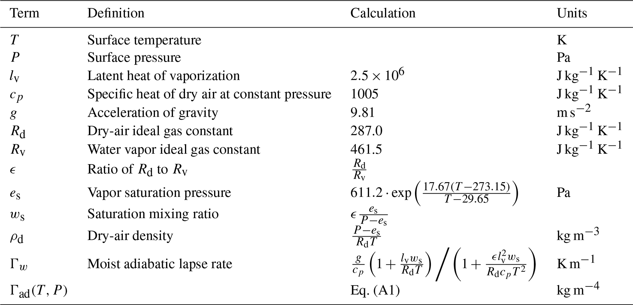
The inverse of the saturation mixing ratio change with height Γad(T,P) is calculated using the formulation published by Albrecht et al. (1990) and Braun et al. (2018), shown in Eq. (A1).
A description and the equations necessary to calculate each term used in the calculation of Γad(T,P) are given in Table A1.
Surface LWC estimation from visibility measurements is done by inverting Eq. (6) in Gultepe et al. (2006). This results in Eq. (B1), where LWC is liquid water content in kilograms per cubic meter and VIS is the visibility in meters.
All data used in this study are hosted by the SIRTA observatory. Data access can be requested for free following the conditions indicated in the SIRTA data policy (https://sirta.ipsl.fr/data_policy.html, last access: 27 August 2021; SIRTA observatory website: https://sirta.ipsl.fr/, last access: 27 August 2021; data request form: https://sirta.ipsl.fr/data_form.html, last access: 27 August 2021).
The supplement related to this article is available online at: https://doi.org/10.5194/acp-21-13099-2021-supplement.
FT and MH developed the conceptual model and its formulation, based on initial work by EW and MH. FT and EW developed the code used for data analysis. FT and MH defined the paper structure and content. MH and JCD manage the SIRTA observatory, which provided the dataset used. All authors reviewed the paper.
The authors declare that they have no conflict of interest.
Publisher’s note: Copernicus Publications remains neutral with regard to jurisdictional claims in published maps and institutional affiliations.
We acknowledge all the SIRTA observatory technical team for their extraordinary work on retrieving long-term and high-quality datasets. SIRTA measurements were performed in the framework of ACTRIS, supported by the European Commission under the Horizon 2020 – Research and Innovation Framework Programme, H2020-INFRADEV-2019-2. We also acknowledge Marc-Antoine Drouin and Cristophe Boitel of the SIRTA observatory for their help on data access. Finally, this publication is based upon work from COST Action PROBE, supported by COST (European Cooperation in Science and Technology).
This research has been supported by the École Polytechnique, Université Paris-Saclay (grant no. LMD2829). It has also been funded by the French Association Nationale Recherche Technologie (ANRT) and the company Meteomodem.
This paper was edited by Barbara Ervens and reviewed by two anonymous referees.
Albrecht, B. A., Fairall, C. W., Thomson, D. W., White, A. B., Snider, J. B., and Schubert, W. H.: Surface-based remote sensing of the observed and the Adiabatic liquid water content of stratocumulus clouds, Geophys. Res. Lett., 17, 89–92, https://doi.org/10.1029/GL017i001p00089, 1990. a, b, c
Bergot, T.: Small-scale structure of radiation fog: a large-eddy simulation study, Q. J. Roy. Meteor. Soc., 139, 1099–1112, 2013. a
Bergot, T.: Large-eddy simulation study of the dissipation of radiation fog, Q. J. Roy. Meteor. Soc., 142, 1029–1040, 2016. a
Betts, A. K.: Cloud Thermodynamic Models in Saturation Point Coordinates, J. Atmos. Sci., 39, 2182–2191, https://doi.org/10.1175/1520-0469(1982)039<2182:CTMISP>2.0.CO;2, 1982. a, b, c
Boers, R. and Mitchell, R. M.: Absorption feedback in stratocumulus clouds influence on cloud top albedo, Tellus A, 46, 229–241, 1994. a, b, c, d
Boers, R., Melfi, S. H., and Palm, S. P.: Cold-Air Outbreak during GALE: Lidar Observations and Modeling of Boundary Layer Dynamics, Mon. Weather Rev., 119, 1132–1150, 1990. a, b, c
Boutle, I., Price, J., Kudzotsa, I., Kokkola, H., and Romakkaniemi, S.: Aerosol–fog interaction and the transition to well-mixed radiation fog, Atmos. Chem. Phys., 18, 7827–7840, https://doi.org/10.5194/acp-18-7827-2018, 2018. a
Braun, R. A., Dadashazar, H., MacDonald, A. B., Crosbie, E., Jonsson, H. H., Woods, R. K., Flagan, R. C., Seinfeld, J. H., and Sorooshian, A.: Cloud Adiabaticity and Its Relationship to Marine Stratocumulus Characteristics Over the Northeast Pacific Ocean, J. Geophys. Res.-Atmos., 123, 13790–13806, https://doi.org/10.1029/2018JD029287, 2018. a, b, c, d, e
Brenguier, J.-L., Pawlowska, H., Schüller, L., Preusker, R., Fischer, J., and Fouquart, Y.: Radiative properties of boundary layer clouds: Droplet effective radius versus number concentration, J. Atmos. Sci., 57, 803–821, 2000. a
Brown, R. and Roach, W.: The physics of radiation fog: II–a numerical study, Q. J. Roy. Meteor. Soc., 102, 335–354, 1976. a, b, c
Cermak, J. and Bendix, J.: Detecting ground fog from space – a microphysics-based approach, Int. J. Remote Sens., 32, 3345–3371, https://doi.org/10.1080/01431161003747505, 2011. a, b, c, d, e, f, g, h, i
Delanoë, J., Protat, A., Vinson, J., Brett, W., Caudoux, C., Bertrand, F., Parent du Chatelet, J., Hallali, R., Barthes, L., Haeffelin, M., and Dupont, J.: Basta: a 95-GHz fmcw doppler radar for cloud and fog studies, J. Atmos. Ocean. Tech., 33, 1023–1038, 2016. a, b
Driedonks, A. and Duynkerke, P.: Current problems in the stratocumulus-topped atmospheric boundary layer, Bound.-Lay. Meteorol., 46, 275–303, 1989. a
Dupont, J.-C., Haeffelin, M., Protat, A., Bouniol, D., Boyouk, N., and Morille, Y.: Stratus–fog formation and dissipation: a 6-day case study, Bound.-Lay. Meteorol., 143, 207–225, 2012. a
Gultepe, I., Müller, M. D., and Boybeyi, Z.: A New Visibility Parameterization for Warm-Fog Applications in Numerical Weather Prediction Models, J. Appl. Meteorol. Climatol., 45, 1469–1480, https://doi.org/10.1175/JAM2423.1, 2006. a, b
Gultepe, I., Tardif, R., Michaelides, S., Cermak, J., Bott, A., Bendix, J., Müller, M. D., Pagowski, M., Hansen, B., Ellrod, G., Jacobs, W., Toth, G., and Cober, S. G.: Fog research: A review of past achievements and future perspectives, Pure Appl. Geophys., 164, 1121–1159, 2007. a
Görsdorf, U., Knist, C., and Lochmann, M.: First results of the cloud radar and microwave radiometer comparison campaign at Lindenberg, ACTRIS Week 2020, available at: https://www.actris.eu/news-events/events/actris-week (last access: 27 August 2021), 2020. a
Haeffelin, M., Barthès, L., Bock, O., Boitel, C., Bony, S., Bouniol, D., Chepfer, H., Chiriaco, M., Cuesta, J., Delanoë, J., Drobinski, P., Dufresne, J.-L., Flamant, C., Grall, M., Hodzic, A., Hourdin, F., Lapouge, F., Lemaître, Y., Mathieu, A., Morille, Y., Naud, C., Noël, V., O'Hirok, W., Pelon, J., Pietras, C., Protat, A., Romand, B., Scialom, G., and Vautard, R.: SIRTA, a ground-based atmospheric observatory for cloud and aerosol research, Ann. Geophys., 23, 253–275, https://doi.org/10.5194/angeo-23-253-2005, 2005. a
Haeffelin, M., Bergot, T., Elias, T., Tardif, R., Carrer, D., Chazette, P., Colomb, M., Drobinski, P., Dupont, E., Dupont, J.-C., Gomes, L., Musson-Genon, L., Pietras, C., Plana-Fattori, A., Protat, A., Rangognio, J., Raut, J.-C., Rémy, S., Richard, D., Sciare, J., and Zhang, X.: PARISFOG: Shedding new light on fog physical processes, B. Am. Meteorol. Soc., 91, 767–783, 2010. a, b
Haeffelin, M., Laffineur, Q., Bravo-Aranda, J.-A., Drouin, M.-A., Casquero-Vera, J.-A., Dupont, J.-C., and De Backer, H.: Radiation fog formation alerts using attenuated backscatter power from automatic lidars and ceilometers, Atmos. Meas. Tech., 9, 5347–5365, https://doi.org/10.5194/amt-9-5347-2016, 2016. a
Hoffmann, H.-E. and Roth, R.: Cloudphysical parameters in dependence on height above cloud base in different clouds, Meteorol. Atmos. Phys., 41, 247–254, 1989. a
Kotthaus, S., O'Connor, E., Münkel, C., Charlton-Perez, C., Haeffelin, M., Gabey, A. M., and Grimmond, C. S. B.: Recommendations for processing atmospheric attenuated backscatter profiles from Vaisala CL31 ceilometers, Atmos. Meas. Tech., 9, 3769–3791, https://doi.org/10.5194/amt-9-3769-2016, 2016. a
Manton, M.: The physics of clouds in the atmosphere, Rep. Prog. Phys., 46, 1393–1444, 1983. a
Marke, T., Ebell, K., Löhnert, U., and Turner, D. D.: Statistical retrieval of thin liquid cloud microphysical properties using ground-based infrared and microwave observations, J. Geophys. Res.-Atmos., 121, 14558–14573, https://doi.org/10.1002/2016JD025667, 2016. a
Mazoyer, M., Lac, C., Thouron, O., Bergot, T., Masson, V., and Musson-Genon, L.: Large eddy simulation of radiation fog: impact of dynamics on the fog life cycle, Atmos. Chem. Phys., 17, 13017–13035, https://doi.org/10.5194/acp-17-13017-2017, 2017. a
Nakanishi, M.: Large-eddy simulation of radiation fog, Bound.-Lay. Meteorol., 94, 461–493, 2000. a
Oliver, D., Lewellen, W., and Williamson, G.: The interaction between turbulent and radiative transport in the development of fog and low-level stratus, J. Atmos. Sci., 35, 301–316, 1978. a
Porson, A., Price, J., Lock, A., and Clark, P.: Radiation fog. Part II: Large-eddy simulations in very stable conditions, Bound.-Lay. Meteorol., 139, 193–224, 2011. a, b
Price, J.: Radiation fog. Part I: observations of stability and drop size distributions, Bound.-Lay. Meteorol., 139, 167–191, 2011. a, b
Price, J., Porson, A., and Lock, A.: An observational case study of persistent fog and comparison with an ensemble forecast model, Bound.-Lay. Meteorol., 155, 301–327, 2015. a
Roach, W., Brown, R., Caughey, S., Crease, B., and Slingo, A.: A field study of nocturnal stratocumulus: I. Mean structure and budgets, Q. J. Roy. Meteor. Soc., 108, 103–123, 1982. a
Roach, W. T., Brown, R., Caughey, S. J., Garland, J. A., and Readings, C. J.: The physics of radiation fog: I – a field study, Q. J. Roy. Meteor. Soc., 102, 313–333, https://doi.org/10.1002/qj.49710243204, 1976. a
Román-Cascón, C., Steeneveld, G. J., Yagüe, C., Sastre, M., Arrillaga, J. A., and Maqueda, G.: Forecasting radiation fog at climatologically contrasting sites: evaluation of statistical methods and WRF, Q. J. Roy. Meteor. Soc., 142, 1048–1063, https://doi.org/10.1002/qj.2708, 2016. a
Slingo, A., Brown, R., and Wrench, C.: A field study of nocturnal stratocumulus; III. High resolution radiative and microphysical observations, Q. J. Roy. Meteor. Soc., 108, 145–165, 1982. a, b, c
Smith, D. K. E., Renfrew, I. A., Price, J. D., and Dorling, S. R.: Numerical modelling of the evolution of the boundary layer during a radiation fog event, Weather, 73, 310–316, https://doi.org/10.1002/wea.3305, 2018. a
Tardif, R. and Rasmussen, R. M.: Event-based climatology and typology of fog in the New York City region, J. Appl. Meteorol. Clim., 46, 1141–1168, 2007. a, b
Wærsted, E.: Description of physical processes driving the life cycle of radiation fog and fog–stratus transitions based on conceptual models, PhD thesis, Paris Saclay, 2018. a, b, c
Wærsted, E. G., Haeffelin, M., Dupont, J.-C., Delanoë, J., and Dubuisson, P.: Radiation in fog: quantification of the impact on fog liquid water based on ground-based remote sensing, Atmos. Chem. Phys., 17, 10811–10835, https://doi.org/10.5194/acp-17-10811-2017, 2017. a, b, c, d, e
Wærsted, E. G., Haeffelin, M., Steeneveld, G.-J., and Dupont, J.-C.: Understanding the dissipation of continental fog by analysing the LWP budget using idealized LES and in situ observations, Q. J. Roy. Meteor. Soc., 145, 784–804, https://doi.org/10.1002/qj.3465, 2019. a, b, c, d, e, f, g, h
Walker, M.: The science of weather: Radiation fog and steam fog, Weather, 58, 196–197, 2003. a
Zhou, B. and Ferrier, B. S.: Asymptotic analysis of equilibrium in radiation fog, J. Appl. Meteorol. Clim., 47, 1704–1722, 2008. a
- Abstract
- Introduction
- Fog conceptual model
- Dataset and data treatment methodology
- Data analysis and results
- Fog life cycle
- Conclusions
- Appendix A: Calculation of Γad(T,P)
- Appendix B: Visibility–LWC parametrization
- Data availability
- Author contributions
- Competing interests
- Disclaimer
- Acknowledgements
- Financial support
- Review statement
- References
- Supplement