Evidence of a recent decline in UK emissions of hydrofluorocarbons determined by the InTEM inverse model and atmospheric measurements

National greenhouse gas inventories (GHGIs) are submitted annually to the United Nations Framework Convention on Climate Change (UNFCCC). They are estimated in compliance with Intergovernmental Panel on Climate Change (IPCC) methodological guidance using activity data, emission factors and facility-level measurements. For some sources, the outputs from these calculations are very uncertain. Inverse modelling techniques that use high-quality, long-term measurements of atmospheric gases have been developed to provide independent verification of national GHGIs. This is considered good practice by the IPCC as it helps national inventory compilers to verify reported emissions and to reduce emission uncertainty. Emission estimates from the InTEM (Inversion Technique for Emission Modelling) model are presented for the UK for the hydrofluorocarbons (HFCs) reported to the UNFCCC (HFC-125, HFC-134a, HFC-143a, HFC-152a, HFC-23, HFC-32, HFC-227ea, HFC-245fa, HFC-43-10mee and HFC-365mfc). These HFCs have high global warming potentials (GWPs), and the global background mole fractions of all but two are increasing, thus highlighting their relevance to the climate and a need for increasing the accuracy of emission estimation for regulatory purposes. This study presents evidence that the long-term annual increase in growth of HFC-134a has stopped and is now decreasing. For HFC-32 there is an early indication, its rapid global growth period has ended, and there is evidence that the annual increase in global growth for HFC-125 has slowed from 2018. The inverse modelling results indicate that the UK implementation of European Union regulation of HFC emissions has been successful in initiating a decline in UK emissions from 2018. Comparison of the total InTEM UK HFC emissions in 2020 with the average from 2009–2012 shows a drop of 35 %, indicating progress toward the target of a 79 % decrease in sales by 2030. The total InTEM HFC emission estimates (2008–2018) are on average 73 (62–83) % of, or 4.3 (2.7–5.9) Tg CO₂-eq yr⁻¹ lower than, the total HFC emission estimates from the UK GHGI. There are also significant discrepancies between the two estimates for the individual HFCs.

1 Introduction

Global emissions of hydrofluorocarbons (HFCs) have been growing rapidly over the last 3 decades as they replace ozone-depleting chlorofluorocarbons (CFCs) and hydrochlorofluorocarbons (HCFCs) in air conditioning, refrigeration, foam-blowing, aerosol propellants and fire retardant applications. CFCs have been phased out globally, and HCFCs are currently being phased out under the Montreal Protocol on Substances that Deplete the Ozone Layer (UNEP, 1987). The Montreal Protocol (MP) is a landmark multilateral environmental agreement that regulates the production and consumption of nearly 100 human-made ozone-depleting substances (ODSs). It has been very successful in preventing further damage to the stratospheric ozone layer, hence protecting humans and the environment from harmful levels of solar ultraviolet radiation. HFCs were introduced as non-ozone-depleting alternatives to support the timely phasing out of CFCs and HCFCs and are now in widespread use. While HFCs do not destroy stratospheric ozone, they are, however, potent greenhouse gases with large global warming potentials (GWPs). Global emissions of HFCs are 0.88 Gt CO₂-eq yr⁻¹ and are comparable to both CFCs, 0.8 Gt CO₂-eq yr⁻¹, and HCFCs, 0.76 Gt CO₂-eq yr⁻¹ (where total global emissions are derived from a budget analysis of measured mole fractions at remote sites based on 2016 data; Montzka et al., 2018b). HFC emissions in recent years represent approximately 1.5 % of the sum of all emissions of long-lived greenhouse gases.

Internationally, HFCs are included in the Kyoto Protocol (KP) (Breidenich et al., 1998) to the United Nations Framework Convention on Climate Change (UNFCCC) as part of a nation's overall greenhouse gas emissions. However the KP was not ratified by all countries, and even where it was, there were no mandatory controls under the KP on HFCs specifically.

The UNFCCC places requirements on developed countries to provide detailed annual inventory reports of their emissions. The 42 countries that make up this group are referred to as Annex-I countries. The UNFCCC requirement is for so-called “bottom-up” reporting, with countries providing estimates of emissions from production, in-use and end-of-life phases. Each element has an emission factor and information on the amount of in-country activity. Due to the significant GWPs of HFCs, uncontrolled growth in emissions poses a challenge to efforts to minimize global temperature rise. With their shorter atmospheric lifetimes compared with carbon dioxide, rapid reductions in HFCs could be advantageous in slowing the rate of climate change in the first half of this century, before CO₂ reduction measures take effect (Xu et al., 2013).

The phasing out of ODSs by the MP has led to more of a reduction of GHG emissions than the KP, but the increased use of HFCs threatens to erode this climate benefit. Therefore, HFCs were added under the Kigali Amendment to the MP in 2016 with most developed countries approving timelines to achieve an 85 % reduction in their production and consumption between 2019 and 2036. Most developing countries will follow with a freeze of HFC consumption levels in 2024 and a final phase-down step of 80 % to 85 % in 2047. HFC-23, emitted predominately as a waste product of HCFC-22 production, is discussed separately in the Supplement. Slightly modified schedules exist for several countries. The Kigali Amendment came into force on 1 January 2019 for those countries that have ratified the amendment. By December 2020, 112 countries had ratified the amendment.

In addition, the European Union (EU) has focused its efforts on reducing emissions of HFCs, along with the other F gases, perfluorocarbons (PFCs) and sulfur hexafluoride (SF₆), through two regulations which pre-date the Kigali Amendment: the 2006 Mobile Air Conditioning (MAC) directive (EU, 2006) and the 2014 F-gas Regulation (EU, 2014). The 2006 EU MAC directive introduced a phased approach to ultimately ban the use of HFCs with global warming potentials on a 100-year time frame (GWP₁₀₀) of over 150 in passenger cars and light commercial vehicles. The most common refrigerant used for this application was HFC-134a with a GWP₁₀₀ of 1360 (Montzka et al., 2018b). Since the implementation of phase three of this directive, on 1 January 2017, the use of fluorinated greenhouse gases with a GWP₁₀₀ of greater than 150 has been banned in all new models of cars and light vans sold in the EU. The 2014 F-gas Regulation, which came into effect in January 2015, aims to cut EU F-gas emissions by two-thirds by 2030, using a progressive quota-based system. A market-driven approach, based on a GWP-weighted phase-down of the quantity of HFCs that can be placed on the EU market, is designed to increase the usage of lower GWP alternatives. In the UK this regulation came into force in March 2015 with the Fluorinated Greenhouse Gases Regulations (UK, 2015).

Understanding the impact and effectiveness of policies on the atmospheric abundance of these gases is vitally important to policy makers to demonstrate the effectiveness of their policies. “Top-down” approaches to estimate emissions have been demonstrated for many different gases (Nisbet and Weiss, 2010; Weiss and Prinn, 2011; Lunt et al., 2015; Bergamaschi et al., 2015; Say et al., 2021) using high-quality, high-frequency atmospheric measurement data and inverse modelling to provide an alternative and complementary method to the traditional bottom-up method. This type of independent emissions verification is considered good practice by the Intergovernmental Panel on Climate Change (IPCC, 2006, 2019), as it assists inventory compilers by identifying inconsistencies between the two approaches (Say et al., 2016) and thereby has the potential to improve the accuracy and reduce the uncertainty of the nationally reported inventories. The atmospheric top-down approach can also give policy makers a more up-to-date assessment of emissions as the bottom-up, inventory-based approach has a built-in publishing time lag of 1 to 2 years.

There is a gap between the total HFC emissions reported by the UNFCCC and the total global emissions derived from atmospheric measurements as reported by Rigby et al. (2014) and Montzka et al. (2018b). Evidence from atmospheric observations has suggested that this gap is largely due to emissions from non-reporting (non-Annex-1) countries, although discrepancies have been found at a gas-specific level between top-down and bottom-up reports for Annex-1 countries (Lunt et al., 2015). A recent study of European emissions covering the period 2008–2014 (Graziosi et al., 2017) reports the status of HFC emissions at a European scale, preceding phase-down, and finds consistency between inventory reported and top-down emissions estimates when the HFCs are aggregated; however, when they considered individual compounds at a country level discrepancies existed between the bottom-up and top-down estimates. A regional study in the USA (covering 2008–2014) also found that aggregated emissions of six HFCs agreed well (within estimated uncertainties) with reported USA inventory estimates (Hu et al., 2017).

The UK is committed to phasing down the sales of HFCs to 21 % by 2030 (Annex V, EU, 2014), based on the average use between 2009–2012. This initiative requires accurate and complete estimates of past and current emissions, which previous studies (Lunt et al., 2015) have shown contain significant uncertainties. Brunner et al. (2017) report a study of four inverse modelling systems (including the system presented here) over Europe in 2011, presenting results for the highest two emitting HFCs by CO₂-eq, HFC-134a and HFC-125, and for SF₆. They compared the top-down estimates for a range of different countries to those reported to the UNFCCC. They concluded that the European network of data available at that time, Mace Head, Jungfraujoch and Monte Cimone, had the potential to identify significant shortcomings in nationally reported emissions but that a denser network would be needed for more reliable modelling across Europe, as the top-down estimates and their uncertainties varied considerably across the four models for some countries.

The aim of this current work is to report, and apply, an updated version of the InTEM (Inversion Technique for Emission Modelling) (Manning et al., 2011) model to estimate both the emissions and the uncertainties of the emissions for 10 HFCs over the UK to enable comparison with the bottom-up estimates submitted by the UK to the UNFCCC. In addition to the atmospheric data used by Brunner et al. (2017), this study uses atmospheric data from three further rural stations (Carnsore Point in Ireland, Taunus in Germany and Tacolneston in the east of the UK) which enhance (see Supplement) the ability to estimate UK emissions and allow for an insight into the spatial distribution of those emissions within the UK. This work is focused purely on reporting emissions from the UK; future work will expand the emission estimates to a wider European region.

2 Methods

2.1 Atmospheric measurements

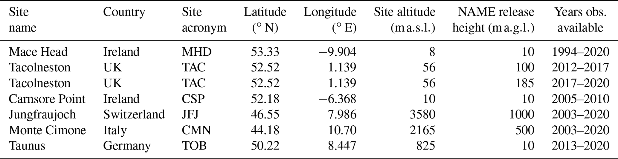
The inverse modelling technique relies on high-quality, long-term measurements of atmospheric gases. In this study, data from six different measuring stations have been used. Four of the measurement stations, Mace Head (MHD; located on the west coast of Ireland), Tacolneston (TAC; East Anglia, England, UK), Jungfraujoch (JFJ; Swiss Alps, Switzerland) and Monte Cimone (CMN; Northern Apennines, Italy), are part of the Advanced Global Atmospheric Gases Experiment (AGAGE) (Prinn et al., 2018). MHD and TAC are also part of a group of observation stations called the UK Deriving Emissions linked to Climate Change (DECC) network (Stanley et al., 2018). Much of the time the MHD measurement station monitors clean westerly air that has travelled across the North Atlantic Ocean. However, when the winds are easterly, it receives substantial regional-scale pollution in air that has travelled from the populated and industrial regions of Europe. The site is therefore uniquely situated to record trace gas concentrations associated with both the Northern Hemisphere background levels and with the more polluted air arising from European emissions. Additionally data have been used from Taunus (TOB) in south-west Germany (Schuck et al., 2018) and Carnsore Point (CSP) on the east coast of Ireland (Dwyer, 2013; Saikawa et al., 2012). Table 2 and the Supplement detail the data availability and measurement information from each site. The measurements of each gas are reported on the same, gas-specific, AGAGE calibration scale irrespective of station.

Table 1 Resolutions of the meteorological models used by NAME. The high-resolution model over the UK and Ireland is nested within the available global model both horizontally and vertically.

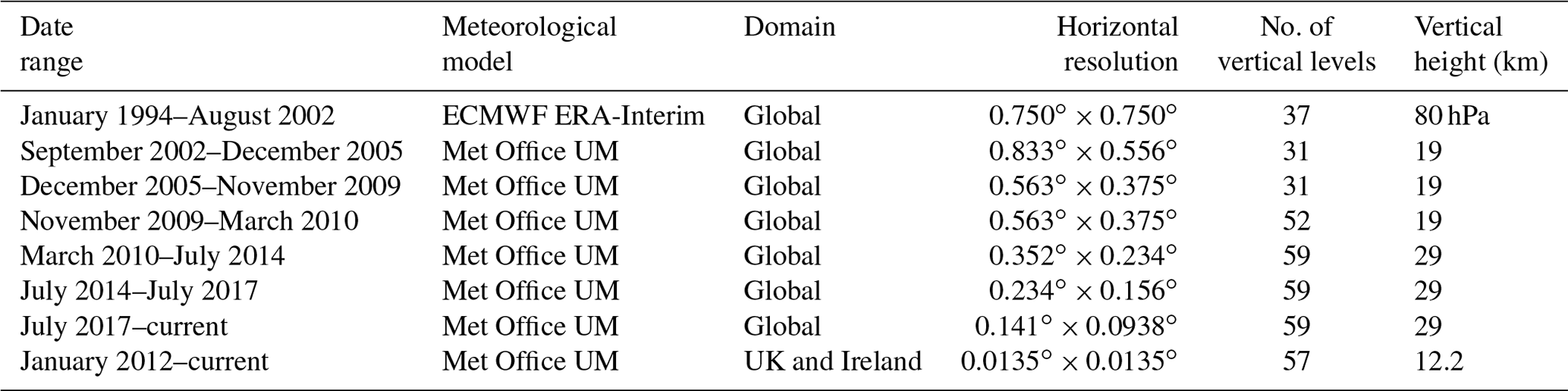
Table 2 Observation site information. Note that the NAME release heights are dependent on the height of the observation inlet above ground, and site altitude is given in metres above sea level ($\mathrm{m}\mathrm{a}.\mathrm{s}.\mathrm{l}.$).

2.2 Atmospheric model

The inversion model InTEM requires calculations of how gases disperse in the atmosphere. In this work the Numerical Atmospheric dispersion Modelling Environment (NAME) (Jones et al., 2007), a Lagrangian atmospheric transport model developed by the UK Met Office, was used to describe the dilution of emissions from source to measurement location. NAME has been used for this type of work in many studies (Manning et al., 2011; Say et al., 2016; Lunt et al., 2018; Montzka et al., 2018a; White et al., 2019; Ganesan et al., 2020; Say et al., 2021; Fraser et al., 2020) and comprehensive details can be found in Arnold et al. (2018). NAME uses a three-dimensional description of the atmosphere as calculated by meteorological models. The meteorological data were obtained from different sources depending on the year, and over the years, the resolutions, both horizontal and vertical, have improved. Table 1 details the evolution of the models used. From 2012, the high-resolution meteorological model over the UK and Ireland has been nested within the available global model. The NAME particle release details for each observation station are given in Table 2. The two high-altitude stations, JFJ and CMN, pose an additional challenge for atmospheric modelling because of the more complex mountain meteorology surrounding each site. In order to compensate for this, the NAME particles were released away from the model surface to reflect that the surface altitudes of the stations in the meteorological models are considerably lower than reality. This is a pragmatic approximation until the resolution of the meteorological models more accurately describe the flow around these stations. The release heights chosen, 1000 m above ground level (a.g.l.) for JFJ and 500 $\mathrm{m}\mathrm{a}.\mathrm{g}.\mathrm{l}.$ for CMN, are arbitrary but are similar to the values used in other research (Brunner et al., 2017; Say et al., 2021). NAME follows 20 000 inert, theoretical particles per hour, with a unit release rate of 1 g s⁻¹, backwards in time for 30 d or until they leave the computational domain (98.1^∘ W to 39.6^∘ E, 10.6 to 79.2^∘ N). The time and position of the exit location is recorded and used later to help describe the concentration of the air entering the modelled domain. Thus, NAME generates the modelled mole fraction contribution over 30 d from each grid cell within the computational domain at each station for each 4 h period. The grid is defined as 0.352^∘ longitude by 0.234^∘ latitude by 0–40 $\mathrm{m}\mathrm{a}.\mathrm{g}.\mathrm{l}.$ The horizontal resolution is ∼25 km over the UK, thus matching the resolution of the global meteorology 2010–2014. NAME particles are considered inert, allowing no chemistry or deposition, which is consistent with the long atmospheric lifetimes of the gases under consideration here. HFC-152a has the shortest lifetime of 1.6 years; the other HFCs have lifetimes between 5.4 and 228 years (Montzka et al., 2018b). Travel time from the UK to the observation stations is less than 5 d for the vast majority of times for all of the stations; therefore, there will be negligible impact due to lifetime on the UK emission estimates even for HFC-152a.

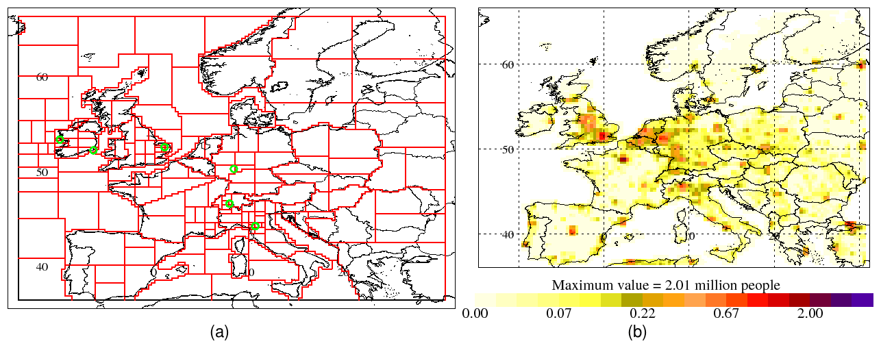
Figure 1 (a) Example grid structure used in InTEM. Green circles denote the locations of the measurement stations. (b) Population per 25 km grid box in units 10⁶ people.

2.3 Inversion framework

Each atmospheric measurement is comprised of two parts: a time-varying background concentration and a perturbation above the background. The perturbations above the background, observed across the network, are driven by emissions on regional scales that have yet to be fully mixed on the hemispheric scale and are the principle information used to estimate surface emissions across north-west Europe. The time-varying Northern Hemisphere background concentration is estimated separately for the three background stations: MHD, JFJ and CMN. For the non-background rural stations, TAC, CSP and TOB, the background time-series estimate for MHD is used as the starting point background concentration (referred to as the “prior”). The method for estimating the background levels used as prior information is described later in this section.

InTEM (Manning et al., 2011; Arnold et al., 2018) has been developed over many years and has been applied to many gases and regions, e.g. Bergamaschi et al. (2018); Park et al. (2021); Mühle et al. (2019); Simmonds et al. (2020); and Fraser et al. (2020). InTEM is used here to estimate UK emissions using the observations described in Table 2. A summary of InTEM model changes from Arnold et al. (2018) to the current InTEM model is provided in the Supplement.

InTEM links the observation time series with each 4 h NAME air history estimate of how surface emissions dilute as they travel to the observation stations. An estimated emission distribution, when combined with the NAME output, can be transformed into a modelled time series of observations at each of the measurement stations. The modelled and the observed time series are compared using statistics to produce a skill score for that particular emission distribution. InTEM uses a Bayesian statistical technique with a non-negative least squares solver (Arnold et al., 2018, and references therein) to find the emission distribution that produces a modelled time series at each observation station that has the best overall statistical match to the observations without allowing the emissions to be negative. The Bayesian method requires the use of a prior emission distribution with associated uncertainties as the starting point for the inversion. The prior information can influence and inform the inversion (posterior) solution. In this work the prior emission information has been distributed over the land area by population density; see Fig. 1 using data from CIESIN (2018). The exception to this is HFC-23, where a uniform land-based prior was used, because HFC-23 emissions are only linked to fugitive releases from industrial processes. The lack of detailed prior spatial and magnitude information is reflected through the use of large prior uncertainties (UK prior uncertainties were set to 100 %; see Sect. 3 for prior emission details for each gas), thus ensuring the inversion results are dominated by the observations and not the prior.

In order for InTEM to be able to provide robust solutions for every area within the modelled domain, each area needs to be identifiable for a sufficient number of times within the inversion period (either 1 or 2 years). If air masses from an area rarely impact the network, then the effect of that area on the statistics is minimal, and the inversion method will have little skill at determining the true emission from there. The contributions different grid cells make to the air concentration at each station varies across the inversion domain; grid boxes that are distant from the observation sites contribute little to the observations, whereas those that are close have a large impact. To balance the contributions from different grid boxes, areas that are more distant are solved for as large regions. Within InTEM the initial grid groupings (regions) are defined using the country boundaries. For each group, the impact of the prior emissions is determined using the NAME dilution matrix. If the number of significant impacts from this region exceeds an arbitrary number (16 times) within the InTEM inversion period (1 or 2 years), then the region is divided in two either vertically or horizontally, determined by maintaining the most equal balance between the two new regions. This process is repeated for both new regions separately until neither satisfies the condition for further splitting or until a region is a single core grid box. The six outermost regions denoting northern Africa, far-eastern Europe, NE Arctic, NW Arctic, Atlantic and the Americas are never split into smaller regions.

Within the inversion process the regions are further refined 24 times, the posterior solution of the previous step is used to estimate the impact of each region, and a single region with the greatest impact is split into two. This secondary process allows a high-magnitude emission area to be identified and ultimately solved as a separate region. After 24 iterations of this process, the regions are fixed and the final InTEM inversion performed. Only the results from the final inversion step are used. Each inversion will potentially have a unique grid of regions because of the availability of different observations in each inversion. An example of the final grid regions used within InTEM is shown in Fig. 1.

For each gas, two sets of inversions are performed, with the inversion time frame being either 1 or 2 calendar years. The 2-year inversions started in the year MHD started observing the gas, the 1-year inversions started in 2013 to coincide with the start of observations from the UK DECC network site TAC. The 2-year inversion periods are necessary pre-2013 to increase the amount of data that the inversion system has to constrain UK posterior emission estimates. The 1-year inversion UK estimates with TAC data give a more realistic, and thus smoother, year-to-year variability in the UK emissions; see Supplement for further information and Table 2 for details of data availability. Every inversion period is repeated 24 times, each time having eight randomly chosen blocks of 5 d of observations per year removed from the data set (equivalent to approximately 10 % of each year). The repeating of each inversion multiple times improves the estimates of uncertainty. Annual emission estimates were made from the 2-year inversions by averaging the inversion results covering each individual year.

Uncertainty in the emissions arises from many factors: errors in the background time-series estimate, emissions that vary over timescales shorter than the inversion time window (diurnal, seasonal or intermittent), heterogeneous emissions within a region, errors in the transport model (NAME) or the underpinning three-dimensional meteorology, or errors in the observations themselves. The potential magnitudes of these uncertainties have been estimated and are incorporated within InTEM to inform the uncertainty of the modelled results and are discussed in more detail in Sect. 2.4.

Time-varying background levels of each gas, as a mole fraction, are estimated as prior information for InTEM for three stations: MHD, JFJ and CMN. In the context of this paper, the background is defined as the mole fraction of the gas as it enters into the defined computational domain, this will be representative of the well-mixed Northern Hemisphere mole fraction adjusted based on the direction and height of the air entering the domain. The prior background mole fractions from MHD are used at CSP, TAC and TOB. However, it is important to note that as the air reaching these stations enters the computational domain from different directions, the prior and posterior background mole fractions at each station will be different from MHD and each other.

For MHD, “background” times are identified when the 30 d air history from NAME is dominated (>80 % of particles) by air from the Atlantic that entered the NAME domain from the western or northern edges. In addition, the amount of population under the entire surface footprint needs to be low, and the amount of land crossed in the local vicinity (within 62.5 km) of the MHD station needs to be small. Using these background times, a polynomial is fitted to the mole fractions; the order of the polynomial is dependent on the number of background times within each moving 6-month window. Considering the resulting background for all (>40) of the gases observed at MHD, background times that have mole fractions that are significantly different to the fitted background for that gas are identified and removed from the set of background times, and then the fitting is completed a second time for all of the gases with this new set of background times. For JFJ and CMN, the background times are defined as times when >80 % of particles are not from the southern border, because of the potential impact of any latitudinal gradient on the background mole fraction, and, like MHD, when the population under the surface footprint is small. The background fitting procedure is otherwise identical to that for MHD. This process generates a time-varying Northern Hemisphere background mole fraction for each gas; see Sect. 3.1. A similar process was used to estimate a northern tropical background using the observations from Ragged Point, Barbados (RPB), and a mid-latitude Southern Hemisphere background using observations from Cape Grim, Australia (CGO) (Prinn et al., 2018).

The accuracy of the meteorology and transport modelling varies with time; therefore, times when either of these are most likely to be poor are excluded from InTEM. This selection process is based on different criteria at the six stations depending on what other information is available. For MHD, CSP, TAC and TOB, the low-altitude stations, times of poorly modelled atmospheric mixing are excluded, such as when the model boundary layer height (BLH) is lower than 300 m, the model BLH and wind speed are strongly varying over the 4 h period, or the modelled atmosphere is strongly stable as determined by the vertical potential temperature gradient. At TAC, where there are CH₄ observations at multiple heights (54, 100 and 185 m), 4 h periods are also removed when the difference between the CH₄ observations at the different heights is greater than a given value (arbitrarily chosen to be 20 ppb). For JFJ and CMN, the two high-altitude stations where the NAME particles are released above the ground, 4 h periods when the modelled BLH is within 100 m of the NAME release point (1000 and 500 $\mathrm{m}\mathrm{a}.\mathrm{g}.\mathrm{l}.$, respectively), are excluded. This process removes between 5 % and 40 % of data depending on site and year.

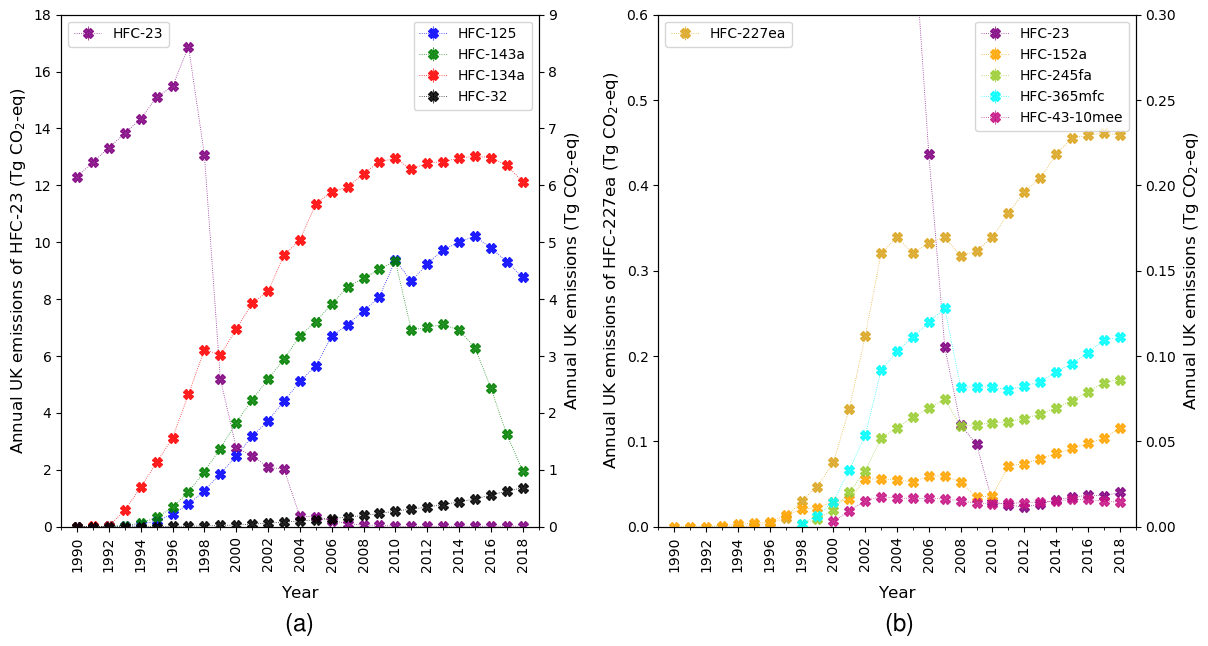
Figure 2 UK HFC inventory emissions (1990–2018) in the 2020 submission to the UNFCCC in Gg yr⁻¹ CO₂-eq. Note the change of scales.

Table 3 Prior multiplying factors for each boundary and their associated uncertainties. See Table 4 for the estimated Tropics Ratios for each gas.

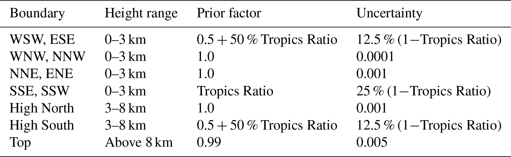
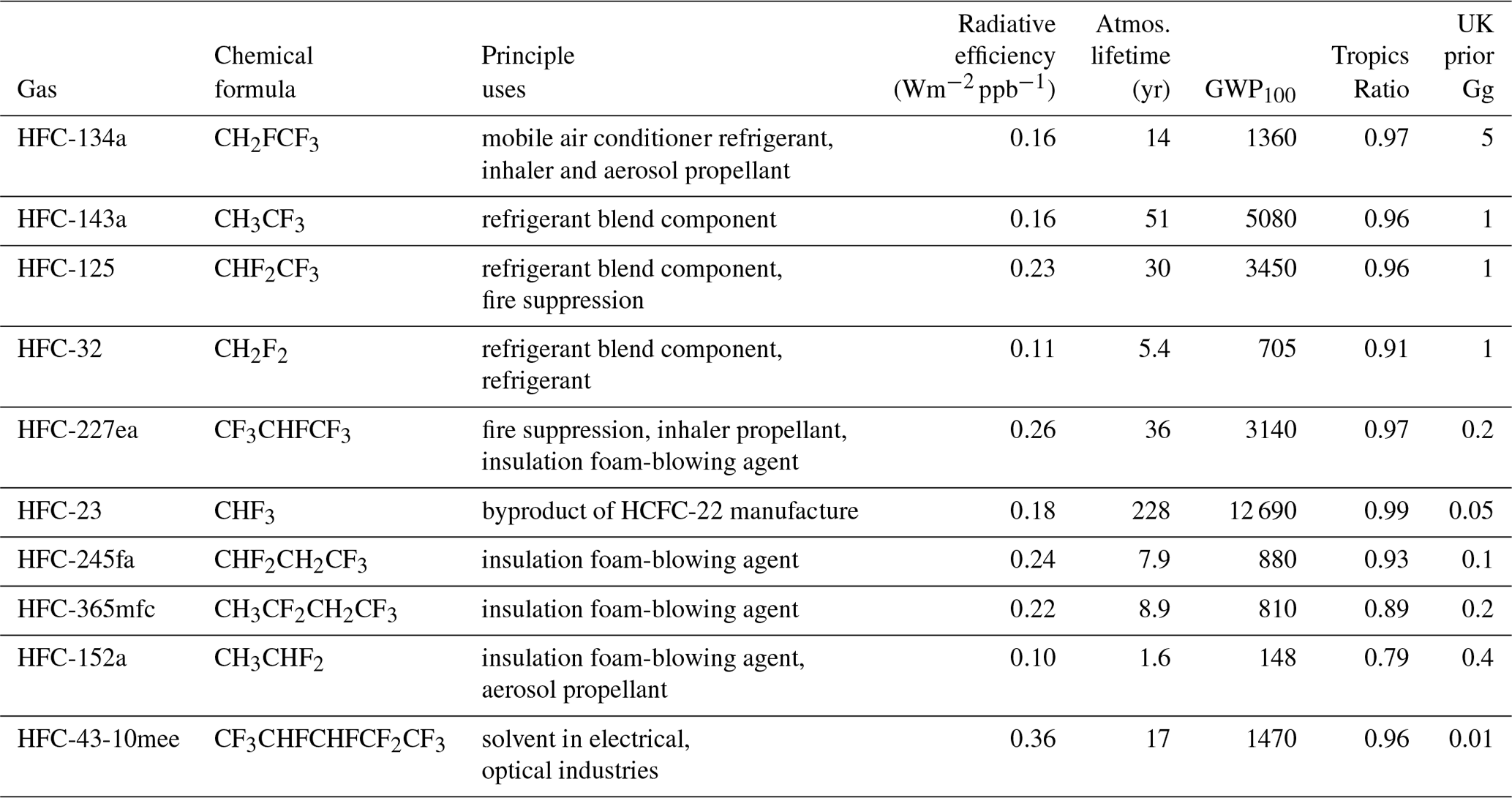
Table 4 Principle uses of each of the HFCs, their radiative efficiency, atmospheric lifetime, global warming potential in a 100-year framework (GWP₁₀₀) (Montzka et al., 2018b), average ratio of mole fraction between the northern tropics (RPB, Barbados) and the northern mid-latitudes (MHD, Ireland) and InTEM prior UK emissions.

There are 11 boundaries encompassing the computational domain which are adjusted independently. They are described in detail in Fig. 2 of Arnold et al. (2018); however, note that the lower boundary in the current study is now 3 km above ground and the upper boundary is now 3–8 km. The fraction of air entering from each boundary is calculated from NAME and multiplied by the solved-for adjustment factor and the prior background mole fraction. This means that each station has a unique solved-for background mole fraction. The prior multiplying factors for each direction are described in Table 3. The air entering from the southern boundary is strongly influenced by tropical and southern hemispheric air masses. The mole fractions of such air masses are lower due to smaller emission rates in the Southern Hemisphere and slow interhemispheric mixing. The average annual ratio of the background mole fraction between the northern tropics and the northern mid-latitudes is used to estimate a “Tropics Ratio” value in Table 3. The northern tropics background is estimated from the observations at RPB (Barbados), and the northern mid-latitude background is estimated from the observations at MHD (Ireland). The estimated Tropics Ratio values vary per gas and are given in Table 4. Each station is also given the freedom to have a small bias compared to the other stations. This bias can be either positive or negative; the prior value is zero and the standard deviation is defined, through consideration, as 0.5 % of the average background mole fraction estimated at MHD; e.g. for HFC-134a this equates to ∼0.38 ppt.

2.4 Uncertainties

Estimating prior, model and observation uncertainties is an important part of InTEM and the most challenging. The prior uncertainties for each of the different elements have been discussed above. The daily precision of the observations is estimated by repeatedly measuring the HFCs in the same tank of air. The standard deviation of these measurements is defined as the observation precision uncertainty (σ_o) for that day's observations for that gas at that station. The model uncertainty is defined as having three components: a background uncertainty (σ_b), a meteorological uncertainty (σ_m) and an atmospheric variability uncertainty (σ_v). The background uncertainty is estimated during the fitting of a continuous line of background mole fraction to the selected background observations. The meteorological uncertainty of each 4 h window is proportional (10 %) to the magnitude of the pollution event in that window, with an imposed minimum uncertainty set to the median pollution event for that gas for that year at that station. The atmospheric variability of the observations within a 12 h window, centred on each 4 h InTEM sample period, makes up the third element. An accurate assessment of the overall model and observation uncertainty is not possible; therefore, judgement was necessary to derive these arbitrary components, at all times attempting to ensure that the uncertainty is sufficiently large to prevent a level of certainty being implied that is unjustified. The overall model and observation uncertainty for each 4 h period (σ_t) is given by Eq. (1).

$$\begin{array}{}\text{(1)}& {\displaystyle }{\displaystyle }{\mathit{\sigma }}_t=\sqrt{{{\mathit{\sigma }}_{\mathrm{o}}}^{\mathrm{2}}+{{\mathit{\sigma }}_{\mathrm{b}}}^{\mathrm{2}}+{{\mathit{\sigma }}_{\mathrm{m}}}^{\mathrm{2}}+{{\mathit{\sigma }}_{\mathrm{v}}}^{\mathrm{2}}}\end{array}$$

3 Results and discussion

A summary of the HFCs observed in the network that are reported to the UNFCCC is given in Table 4, together with their principle uses, radiative efficiency, atmospheric lifetime and GWP₁₀₀. The UK's 2020 submission of HFC emissions to the UNFCCC (which provide values up to and including 2018) have been scaled by their respective GWP₁₀₀ values (Table 4) and are shown in Fig. 2. Note the change in scales of the y axis between the two panels, which reflects the huge difference in global warming impact from these gases. HFC-23 had the greatest impact of the HFCs until its rapid decline after 1997. From the year 2000 to the most recent submission for 2018, the gases having the biggest effect are HFC-134a, HFC-143a and HFC-125, although as can be seen in Fig. 2, emissions of HFC-143a have rapidly decreased since 2014. In this paper InTEM modelled data are presented for the top five HFCs (HFC-134a, HFC-125, HFC-143a, HFC-32 and HFC-227ea), ranked by annual emission multiplied by GWP₁₀₀, together with the total HFC data for the UK. The InTEM modelled data for the remaining five HFCs are detailed individually in the Supplement.

Figure 3 Northern Hemisphere atmospheric background mole fractions (ppt) of HFCs at the MHD (Ireland) observing station (thick lines) and Southern Hemisphere values at the CGO (Australia) (thin lines). A 1-year smoothing has been applied to the monthly background estimates. The left y axis for plot (a) relates to HFC-134a, and the right axis relates to the other gases shown. The right y axis for plot (b) relates to HFC-43-10mee, and the left axis relates to the other gases shown. Note the change in y scales.

3.1 Background mole fractions

For each of the HFCs, the background analysis, as described in Sect. 2.3, using observations from MHD gives an estimate of the annual mid-latitude Northern Hemisphere background mole fraction as shown in Fig. 3. A similar analysis, using observations from the remote station at CGO in Tasmania, Australia, gives the estimates of the annual mid-latitude Southern Hemisphere background mole fractions. Figure 4 shows the corresponding, 2-year smoothed, annual growth for each gas at both stations. The background mole fractions of all of the HFCs are increasing in both hemispheres, with a time lag of 1–2 years in the Southern Hemisphere. The atmospheric mixing ratios of some of the gases are growing very rapidly, most notably HFC-134a, HFC-125 and HFC-32. The mixing ratios of HFC-43-10mee are growing much more slowly, while HFC-152a has shown little overall growth since 2012 and has even recorded a few years of decline (Fig. 4). The growth of HFC-365mfc in the Northern Hemisphere has fallen steadily since 2015, which is reflected in the mixing ratio (Fig. 3) plateauing in the Northern Hemisphere in 2020. The overall growth of HFC-32, HFC-125, HFC-143a and HFC-227ea has continued to increase over the measurement period, although HFC-143a and HFC-227ea have had periods where the annual growth reduced briefly before then increasing in subsequent years. HFC-32 has shown the most rapid increase in growth of all the HFCs, but in 2020, for the first time, the Northern Hemisphere annual growth is less than that for the previous year, which could be the first indication of a slowdown. HFC-23 and HFC-245fa have, on average, an increasing growth rate but they are not uniformly rising. Figure 4 shows that the growth of HFC-134a, since reaching a peak in 2017 in the Northern Hemisphere and 2018 in the Southern Hemisphere, has undergone a reduction in annual growth in both hemispheres, implying that the global emissions of this gas are currently falling. The Southern Hemisphere annual growth is generally smaller than in the Northern Hemisphere and the trend lags behind by 1–2 years.

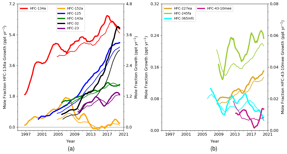
Figure 4 Northern Hemisphere atmospheric background mole fraction growth rates (ppt yr⁻¹) of HFCs at the MHD (Ireland) observing station are shown as thick lines, corresponding Southern Hemisphere values from CGO (Australia) are shown as thin lines. A 2-year smoothing has been applied to the growths that are calculated by subtracting last year's mole fraction from this year's value on a monthly basis. The left y axis for plot (a) relates to HFC-134a, and the right axis relates to the other gases shown. The right y axis for plot (b) relates to HFC-43-10mee, and the left axis relates to the other gases shown. Note the change in y scales.

3.2 HFC-134a

The main uses of HFC-134a are as a refrigerant in mobile air conditioning systems, in metered-dose inhalers and as an aerosol propellant. Globally, the atmospheric abundance of HFC-134a continues to grow; however, the growth in the Northern Hemisphere appears to have peaked in 2017 at 6.5 ppt yr⁻¹ (Fig. 4), dropping to 5.7 ppt yr⁻¹ in 2020. It should be noted, as Fig. 4 shows, there is evidence of previous interannual variability in the growth of HFC-134a, so further years of data will be required to confirm this. In 1997 the northern hemispheric background mole fraction grew at a rate of ∼2 ppt yr⁻¹. Figure 5 presents InTEM emission estimates for HFC-134a up to 2020 for the two model inversion set-ups, as described in Sect. 2.3, here referred to as InTEM-2yr and InTEM-1yr, plotted alongside the UK 2020 inventory submission to the UNFCCC. The InTEM-2yr results show good agreement initially in 1995 and 1996 but thereafter estimate significantly lower emissions than the inventory, though there is good trend agreement with the steady rise in emissions and subsequent levelling off from 2011 onward. The model, however, then diverges again with an increase in 2017 for both InTEM-2yr and InTEM-1yr. The InTEM-1yr results continue to increase in 2018 before a fall of 1.8 Tg CO₂-eq in 2019 which continues to a lesser extent into 2020. The InTEM-2yr result appears to drop sooner, in 2018, but less sharply due to averaging over a longer time frame, which, as previously described, encompasses data from model inversions for 2017–2018 and 2018–2019 to estimate the 2018 result. The InTEM-1yr model result is estimating a drop of 2.0 Tg CO₂-eq from the last reported year in 2018 to 2020. Overall, a significant discrepancy exists between InTEM and the UK inventory estimates, with the inventory higher in all reporting years. Over the last 10 reported years (2009–2018) the inventory is, on average, 2.2 Tg CO₂-eq (54 %) higher than the InTEM estimate (or InTEM is 34 % lower than the inventory). It is possible that there was a change in UK HFC-134a emissions due to the Covid-19 pandemic in 2020; however, the most significant drop in UK emissions occurred in 2019, before the pandemic arrived in the UK. It is probable, therefore, that the Covid-19 impact on UK HFC-134a emissions, if any, was small but ultimately cannot be ascertained yet.

Other inverse studies of HFC-134a have also found that their estimates are lower than the inventory values they were comparing with. Lunt et al. (2015) found that the 2010–2012 average of their HFC-134a estimates for Annex-1 countries was 21 % lower than the UNFCCC inventory, with significant variability across the different countries arising from their different assessments of emission factors and activity data. Say et al. (2016) found a significant discrepancy between UK emissions of HFC-134a when comparing InTEM and the UK inventory as reported in 2014 (with inventory data up to and including 2012). This led to a re-evaluation of the inventory model used for the estimation of emissions from the UK refrigeration and air conditioning sectors. The inventory team adjusted a number of conservative assumptions that had, most likely, contributed to an overestimation of UK HFC-134a inventory emissions. The UK inventory values for HFC-134a shown in Say et al. (2016) were subsequently revised downwards; for example, the 2012 estimate fell by ∼1 Gg yr⁻¹ (∼1.4 Tg CO₂-eq) in the 2016 UK submission and a further ∼0.2 Gg yr⁻¹ (∼0.25 Tg CO₂-eq) in the 2017 submission to the values plotted in Fig. 5. Graziosi et al. (2017) compared emission estimates for HFC-134a, derived using the FLEXPART (FLEXible PARTicle) model combined with a Bayesian inversion method, with the UNFCCC inventories submitted in 2016 (including data up to 2014) for European countries including the UK. They found that their UK emission estimate, averaged over the period 2008–2014, was lower than the inventory by approximately one-third.

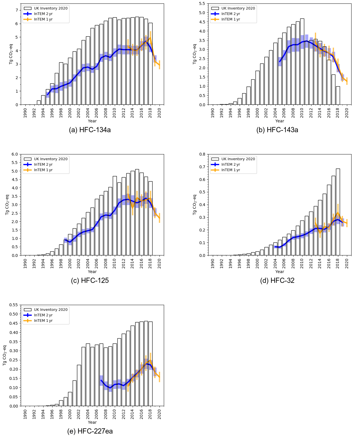
Figure 5 Annual UK emission estimates (Tg CO₂-eq) from the UK 2020 inventory (black), InTEM annualized 2-year inversion (blue) and InTEM 1-year inversion (orange) (a) HFC-134a, (b) HFC-143a, (c) HFC-125, (d) HFC-32 and (e) HFC-227ea. The uncertainty bars represent 1σ.

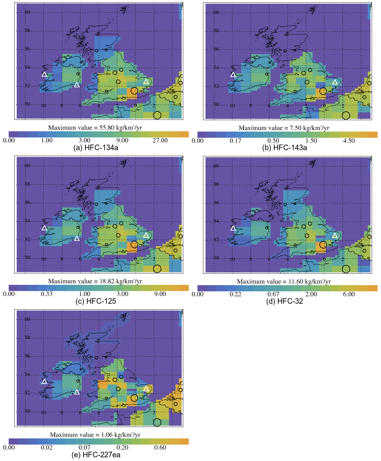
Figure 6 Two-year average InTEM emission estimate 2019–2020 ($\mathrm{kg}{\mathrm{km}}^{-\mathrm{2}}{\mathrm{yr}}^{-\mathrm{1}}$) (a) HFC-134a, (b) HFC-143a, (c) HFC-125, (d) HFC-32 and (e) HFC-227ea. Black circles represent major cities, and white triangles show the locations of the observation sites.

Spatial emission estimates for HFC-134a from the InTEM-1yr model inversions are presented in Fig. 6 for the period 2019–2020. Some major cities are indicated with black circles to allow for orientation, with the area of each circle approximately proportional to the population within the metropolitan area of that city. The variable grid resolution of InTEM, dependant on source signal, produces a patchwork of different resolutions. The highest emissions are generally focused on the more populated areas, with the highest emission region appearing in the south of the UK near to London.

As a sensitivity test, the HFC-134a 1-year inversions were also performed using a uniform land-based (flat) prior. The InTEM 2013–2020 average UK emissions were similar when using the flat prior (4.1 ± 0.45 Tg CO₂-eq) compared to when using the population prior (4.1 ± 0.54 Tg CO₂-eq), showing that there is little dependence on the prior.

3.3 HFC-143a

HFC-143a is used as a component of several refrigerant blends, mainly R-404A. The atmospheric concentration of HFC-143a is increasing globally; however, since 2016 the rate of increase has levelled off (Fig. 4). InTEM modelled UK emissions (Fig. 5) increase rapidly between 2005–2007 (2.3 to 3.2 Tg CO₂-eq) followed by a period of slower growth until 2011 (peaking at 3.5 Tg CO₂-eq), after which emissions begin to decline steadily until 2017 (2.7 Tg CO₂-eq) and then more rapidly until 2020 (1.3 Tg CO₂-eq). The model is ∼28 % below the inventory from 2005 until 2010, when a step change in the inventory brings it into good agreement with InTEM until 2015. The step change in the inventory from 2010–2011 (fall of 1.2 Tg CO₂-eq) can be partly attributed to how the UK inventory team modelled the implementation of an EU law that regulated technicians dealing with specific types of refrigeration systems. In the UK this was modelled as a drop in lifetime leak rates from 2010 onward. From 2016 onwards the inventory decreases more rapidly year-on-year than the InTEM estimates, although both drop sharply. By 2018 the InTEM estimate (2.1 Tg CO₂-eq) is double the inventory value (1.0 Tg CO₂-eq).

The largest UK sources of HFC-143a are associated with populated regions, particularly in the south-east. Figure 6 shows the emission map for the average of 2019 and 2020, when the InTEM annual UK totals have decreased significantly compared with the InTEM modelled peak emission in 2011.

3.4 HFC-125

The atmospheric concentration of HFC-125 is increasing globally. It is used in refrigerant blends for air conditioning (e.g. R-410A and R-407C) and refrigeration (e.g. R-404A) and also as a fire suppressant. Figure 5 shows that UK emission estimates from both the UK inventory and the InTEM model increase steadily over time, with the inventory peaking in 2015 (5.1 Tg CO₂-eq) and the InTEM emissions plateauing 2012–2017 ($\text{average}=\mathrm{3.3}\pm \mathrm{0.4}$ Tg CO₂-eq). The InTEM model estimate is on average 35 % lower than the inventory throughout. The inventory declines slowly from 2015 to 2018, whereas the InTEM estimate remains fairly flat, only starting a rapid decline after 2017 in the InTEM-2yr model and 2018 in the InTEM-1yr model. Figure 6 shows the average InTEM spatial emission map for 2019–2020. Similar to HFC-134a, populated areas are the most significant sources.

3.5 HFC-32

The global atmospheric concentration of HFC-32 is increasing at an accelerating rate, and the interhemispheric gradient is growing (Fig. 3); however, at the very end of the data record there is a slowing of the growth. Future data will show whether this is just a temporary slowdown, possibly as a result of the Covid-19 pandemic, or whether it is indicating a more permanent change. HFC-32 is used both as a pure refrigerant and as a component of refrigerant blends. The UK inventory (Fig. 5) shows an annual accelerating increase in emissions over the reported period, reaching just under 0.7 Tg CO₂-eq in 2018. In contrast, InTEM shows a roughly linear increase from 2005 until 2018, reaching a maximum in the 1-year data in 2018 that is ∼50 % lower than the inventory. The InTEM estimates then decrease in 2019 and 2020. The UK inventory is considerably greater than (on average 1.8 times) InTEM in all reporting years. Figure 6 shows the average emissions for 2019–2020 and indicates that the spatial distribution of HFC-32 emissions largely follows population density.

3.6 HFC-227ea

HFC-227ea is used for fire suppression, as a propellant in metered-dose inhalers and as a foam-blowing agent for insulation. The atmospheric mole fraction is increasing globally and the growth is accelerating, with a widening hemispheric gradient. Figure 5 shows that the UK InTEM emission estimates are on average 0.25 Tg CO₂-eq, or approximately two-thirds (63 %), lower than those reported in the inventory, although the correlation between the trends of the two estimates is reasonable. Similar to the other HFCs reported, InTEM UK emission estimates of HFC-227ea decline markedly from 2018 (0.25 Tg CO₂-eq) to 2020 (0.16 Tg CO₂-eq). The spatial pattern of the InTEM emission estimates are shown in Fig. 6, and they largely follow population, though with more variation in the spatial distribution than is seen in the other HFCs. This effect continues across the years, with high emissions in NE Wales (low population) and NW England (high population) appearing from 2015; high emissions are also observed from the near continent. It is also notable that the statistical fit between the observed and modelled time series in all years, principally at TAC (see Supplement for more details), is significantly worse than for the other gases. The uses of HFC-227ea, e.g. as the UK's dominant HFC fire-suppression gas, means that its emission is potentially much more intermittent, thus making it harder to model. It is also likely to be less tied to population distribution because of its specialist uses. Similar to HFC-134a, a uniform land-based (flat) prior was tested, the results show remarkable similarity (average 2013–2020 UK emissions: 0.19±0.04 Tg CO₂-eq) to the results using the population prior (average 2013–2020 UK emissions: 0.18±0.03 Tg CO₂-eq).

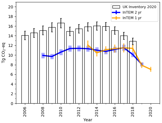
Figure 7 Total UK HFC emission estimates (HFC-125, HFC-134a, HFC-143a, HFC-152a, HFC-23, HFC-32, HFC-227ea, HFC-245fa, HFC-365mfc and HFC-43-10mee) in Tg CO₂-eq yr⁻¹ from the UK inventory submitted to the UNFCCC in 2020 (black), InTEM annualized 2-year inversion (blue) and InTEM 1-year inversion (orange). Note that HFC-43-10mee (<0.02 Tg CO₂-eq yr⁻¹) is included in the InTEM data from 2011 when the observations start. The uncertainty bars represent 1σ.

3.7 Aggregated UK HFCs

All of the HFCs modelled in this study (HFC-23, HFC-245fa, HFC-365mfc, HFC-152a and HFC-43-10mee are shown in the Supplement) have been weighted by their GWP₁₀₀ value and combined to estimate a total UK HFC emission estimate in Tg CO₂-eq yr⁻¹ (Fig. 7). Note that due to the start date of the measurement of HFC-43-10mee, it is only included in the InTEM value from 2011 onwards; however, its contribution (∼0.01 Tg CO₂-eq yr⁻¹) is close to negligible. The total inventory HFC emission for the UK is 14.1 Tg CO₂-eq in 2006 and increases to a maximum of 16.6 Tg CO₂-eq in 2010. The drop in inventory emissions seen from 2010 to 2011 is attributable to the drop in the HFC-143a inventory estimate between those 2 years. From 2011 the inventory then rises gradually, peaking in 2014 (16.0 Tg CO₂-eq), before falling steadily to 12.9 Tg CO₂-eq yr⁻¹ in 2018. The atmospheric measurement data available allow InTEM total UK HFC emissions to be estimated from 2008 onwards. The InTEM-1yr estimates are used in preference to the InTEM-2yr values from 2013. The InTEM estimates are consistently lower, on average by 4.3 (2.7–5.9) Tg CO₂-eq, or 73 (62–83) % of the reported inventory 2008–2018. The InTEM estimates rise gradually until 2011, after which the emissions stay relatively constant (average of 11.3 Tg CO₂-eq) until 2018, apart from a slight dip in 2014–2015. The InTEM estimates then start to decline, dropping to 7.0 Tg CO₂-eq in 2020. The closest agreement between InTEM and the inventory is in 2018. The InTEM estimated drop in total HFC from 2018 to 2020 is 4.3 (3.1–5.6) Tg CO₂-eq. Graziosi et al. (2017) reported ∼11 Tg CO₂-eq total HFC (excluding HFC-23) for the UK as an average from 2008–2014, which is similar to the comparable InTEM estimate of 10.5 (9.8–11.2) Tg CO₂-eq. Lunt et al. (2015) found that whilst overall total HFC emission estimates (averaged across 2010–2012 and Annex-1 countries) were in good agreement with UNFCCC inventory reports, the emissions of individual HFCs were not in good agreement. In line with the conclusions of Lunt et al. (2015), this work shows that it is the cancellation of discrepancies between the InTEM and inventory estimates for the individual gases that generates a better agreement for the total HFC values (Fig. 7) than estimated for the individual gases.

4 Conclusions

This study has shown that the background atmospheric mixing ratios of some HFCs are increasing very rapidly, most notably HFC-134a, HFC-125 and HFC-32, whilst others, HFC-43-10mee, HFC-152a and HFC-365mfc, have shown limited or no recent increase. The overall growth of HFC-32, HFC-125, HFC-143a, HFC-227ea, HFC-23 and HFC-245fa have continued to increase during the measurement period, although most gases have had periods of reduced growth. HFC-32 has shown the most rapid increase in growth of all the HFCs, but for the first time, the growth in 2020 in the Northern Hemisphere is less than that for the previous year. HFC-134a has shown, since reaching a growth peak in 2017 in the Northern Hemisphere and 2018 in the Southern Hemisphere, a reduction in annual growth in both hemispheres, implying that the global emissions of this gas have been falling since 2017.

This study has reported annual emission estimates for the UK for 10 individual HFCs, modelled using the UK Met Office's InTEM model, up to and including 2020, as well as annual estimates of total UK HFC emissions. The five less significant HFCs, based on their impact on the climate after 2003 (UK emissions multiplied by GWP₁₀₀), are detailed in the Supplement. The InTEM estimates show a clear change from flat or increasing UK emissions up to 2018 to a fall in UK emissions in 2019 and 2020 in all of the top five HFCs. There are significant discrepancies between the UK inventory and InTEM estimates in 2018 (currently the latest reported year) for all HFCs, with the InTEM estimates lower in all except HFC-143a and HFC-23. The total InTEM HFC emission estimates (2008–2018) are on average 73 (62–83) % of, or 4.3 (2.7–5.9) Tg CO₂-eq yr⁻¹ lower than, the total HFC emission estimates from the UK GHGI. However, even though the InTEM total is consistently lower, it masks a strong variability in the comparisons of the individual gases with the inventory.

The InTEM results to 2020 are giving a strong indication that the phase-down measures that have been implemented in the UK are having a positive impact. Quantitatively this can be measured by progress towards the target set out in Annex V EU (2014). The total InTEM UK HFC emission in 2020 (7.0 Tg CO₂-eq yr⁻¹) compared with the average InTEM estimate from 2009–2012 (10.8 Tg CO₂-eq yr⁻¹) shows a drop of 35 % in emissions, indicating progress toward the target of a 79 % decrease in sales by 2030. Future work should extend the scope of this study to other European countries which have sufficient sensitivity to the atmospheric measurement sites, to allow for a Europe-wide assessment of the progress towards phasing down HFCs.