the Creative Commons Attribution 4.0 License.
the Creative Commons Attribution 4.0 License.
 | 29 Jan 2021
Technical note: A high-resolution inverse modelling technique for estimating surface CO2 fluxes based on the NIES-TM–FLEXPART coupled transport model and its adjoint
Tomohiro Oda
Makoto Saito
Rajesh Janardanan
Dmitry Belikov
Johannes W. Kaiser
Ruslan Zhuravlev
Alexander Ganshin
Vinu K. Valsala
Arlyn Andrews
Lukasz Chmura
Edward Dlugokencky
László Haszpra
Ray L. Langenfelds
Toshinobu Machida
Takakiyo Nakazawa
Michel Ramonet
Colm Sweeney
Douglas Worthy
We developed a high-resolution surface flux inversion system based on the global Eulerian–Lagrangian coupled tracer transport model composed of the National Institute for Environmental Studies (NIES) transport model (TM; collectively NIES-TM) and the FLEXible PARTicle dispersion model (FLEXPART). The inversion system is named NTFVAR (NIES-TM–FLEXPART-variational) as it applies a variational optimization to estimate surface fluxes. We tested the system by estimating optimized corrections to natural surface CO2 fluxes to achieve the best fit to atmospheric CO2 data collected by the global in situ network as a necessary step towards the capability of estimating anthropogenic CO2 emissions. We employed the Lagrangian particle dispersion model (LPDM) FLEXPART to calculate surface flux footprints of CO2 observations at a spatial resolution of . The LPDM is coupled with a global atmospheric tracer transport model (NIES-TM). Our inversion technique uses an adjoint of the coupled transport model in an iterative optimization procedure. The flux error covariance operator was implemented via implicit diffusion. Biweekly flux corrections to prior flux fields were estimated for the years 2010–2012 from in situ CO2 data included in the Observation Package (ObsPack) data set. High-resolution prior flux fields were prepared using the Open-Data Inventory for Anthropogenic Carbon dioxide (ODIAC) for fossil fuel combustion, the Global Fire Assimilation System (GFAS) for biomass burning, the Vegetation Integrative SImulator for Trace gases (VISIT) model for terrestrial biosphere exchange, and the Ocean Tracer Transport Model (OTTM) for oceanic exchange. The terrestrial biospheric flux field was constructed using a vegetation mosaic map and a separate simulation of CO2 fluxes at a daily time step by the VISIT model for each vegetation type. The prior flux uncertainty for the terrestrial biosphere was scaled proportionally to the monthly mean gross primary production (GPP) by the Moderate Resolution Imaging Spectroradiometer (MODIS) MOD17 product. The inverse system calculates flux corrections to the prior fluxes in the form of a relatively smooth field multiplied by high-resolution patterns of the prior flux uncertainties for land and ocean, following the coastlines and fine-scale vegetation productivity gradients. The resulting flux estimates improved the fit to the observations taken at continuous observation sites, reproducing both the seasonal and short-term concentration variabilities including high CO2 concentration events associated with anthropogenic emissions. The use of a high-resolution atmospheric transport in global CO2 flux inversions has the advantage of better resolving the transported mixed signals from the anthropogenic and biospheric sources in densely populated continental regions. Thus, it has the potential to achieve better separation between fluxes from terrestrial ecosystems and strong localized sources, such as anthropogenic emissions and forest fires. Further improvements in the modelling system are needed as our posterior fit was better than that of the National Oceanic and Atmospheric Administration (NOAA)'s CarbonTracker for only a fraction of the monitoring sites, i.e. mostly at coastal and island locations where background and local flux signals are mixed.
- Article
(4570 KB) - Full-text XML
-
Supplement
(3097 KB) - BibTeX
- EndNote


Inverse modelling of the surface fluxes is implemented by using chemical transport model simulations to match atmospheric observations of greenhouse gases (GHGs). CO2 flux inversion studies started from addressing large-scale flux distributions (Enting and Mansbridge, 1989; Tans et al., 1990; Gurney et al., 2002; Peylin et al., 2013, and others) using background monitoring site data and global transport models at low and medium spatial resolutions, targeting the extraction of the information on large and highly variable fluxes of CO2 from terrestrial ecosystems and oceans. The merits of improving the spatial resolutions of global transport simulations to 9–25 km, which this study aims to demonstrate, have been also discussed by previous studies, such as Agusti-Panareda et al. (2019) and Maksyutov et al. (2008). However, global inverse modelling studies have never been conducted at these spatial resolutions. On the other hand, regional-scale fluxes, such as national emissions of non-CO2 GHGs, have been estimated using inverse modelling tools that rely on regional (mostly Lagrangian) transport algorithms which are capable of resolving surface flux contributions to atmospheric concentrations at resolutions from 1 to 100 km (Vermeulen et al., 1999; Manning et al., 2011; Stohl et al., 2009; Rödenbeck et al., 2009; Henne et al., 2016; He et al., 2018; Schuh et al., 2013; Lauvaux et al., 2016 and others). Extension of the regional Lagrangian inverse modelling to the global scale, based on the combination of the three-dimensional (3-D) global Eulerian model and Lagrangian model, has been implemented in several studies (Rugby et al., 2011; Zhuravlev et al., 2013; Shirai et al., 2017). They have demonstrated an enhanced capability to resolve the regional and local concentration variabilities driven by fine-scale surface emission patterns, while the inverse modelling schemes rely on regional and global basis functions that yield concentration responses of regional fluxes at observational sites. A disadvantage of using the regional basis functions in inverse modelling is the flux aggregation errors, as noted by Kaminski et al. (2001). This has been addressed by developing grid-based inversion schemes based on variational assimilation algorithms that yield flux corrections that are not tied to aggregated flux regions (Rödenbeck et al., 2003; Chevallier et al., 2005; Baker et al., 2006, and others). In order to implement a grid-based inversion scheme that is suitable for optimizing surface fluxes using the high-resolution atmospheric transport capability of the Lagrangian model, an adjoint of a coupled Eulerian–Lagrangian model is needed, as reported by Belikov et al. (2016).
In this study, we applied an adjoint of the coupled Eulerian–Lagrangian transport model, which is a revised version of Belikov et al. (2016), to the problem of surface flux inversion, based on a coupled transport model with a spatial resolution of the Lagrangian model at 0.1∘ longitude–latitude. While global higher-resolution transport simulations can be implemented with coupled Eulerian–Lagrangian models (e.g. Ganshin et al., 2012), the choice of the model resolution in our inversion system was dictated mostly by the availability of the prior surface CO2 fluxes.
The practical need for running high-resolution atmospheric transport simulations at the global scale is currently driven by expanding the GHG-observing capabilities towards quantifying anthropogenic emissions by observing GHGs at the vicinity of emission sources (Nassar et al., 2017; Lauvaux et al., 2020). These include observations in both background and urban sites with tall towers, commercial aeroplanes, and satellites. At the same time, the focus of inverse modelling is evolving towards studies of the anthropogenic emissions, with a target of making better estimates of regional and national emissions in support of national and regional GHG emission reporting and control measures (Manning et al., 2011; Henne et al., 2016; Lauvaux et al., 2020). In that context, global-scale, high-resolution inverse modelling approaches have the advantage of closing global budgets, while regional- and national-scale inverse modelling approaches with limited area models require boundary conditions normally provided by global model simulations with optimized fluxes. Often there is an additional degree of freedom introduced by allowing corrections to the boundary concentration distribution to improve a fit at the observation sites (Manning et al., 2011). As a result, the global total of regional emission estimates does not necessarily match the balance constrained by global mean concentration trends. A global coupled Eulerian–Lagrangian model, such as Ganshin et al. (2012), has the potential to address both the objectives; that is, closing the global balance and operating at the range of scales from a single city (Lauvaux et al., 2016) to a large country or continental scale. Here we report the development of a high-resolution inverse modelling technique that is suitable for application at a broad range of spatial scales. We applied it to the problem of estimating the distribution of CO2 fluxes over the globe that provides the best model fit to the observations. In separate studies, the same inversion system was applied to the inverse modelling of methane emissions (Wang et al., 2019; Janardanan et al., 2020).
The objective of this study is to optimize the natural CO2 fluxes in order to provide background CO2 concentration fields for estimating fossil CO2 emissions where the advantage of the high-resolution approach is more evident. The paper is organized as follows: Sect. 1 provides an introduction, Sect. 2 contains the transport model and its adjoint, Sect. 3 introduces the prior fluxes, observational data set, and gridded flux uncertainties, Sect. 4 gives the formulation of the inverse modelling problem and numerical solution, and Sect. 5 presents the simulation results and discussion, followed by the summary and conclusions.
For the simulation of the CO2 transport in the atmosphere, we used the coupled Eulerian–Lagrangian model NIES-TM–FLEXPART (defined as the National Institute for Environmental Studies transport model coupled with the FLEXible PARTicle dispersion model), which is a modified version of the model described by Belikov et al. (2016). The coupled transport model is computationally more efficient in comparison to the Eulerian model if both models are run on the same spatial resolution. Belikov et al. (2016) confirmed that the coupled model with a Lagrangian model resolution of performs similarly when coupled with Eulerian model at either a or resolution, and performance degradation was only seen when using a resolution Eulerian model. The coupled model consists of NIES-TM v08.1i, with a horizontal resolution of and 32 hybrid–isentropic vertical levels (Belikov et al., 2013), and the FLEXPART model v.8.0 (Stohl et al., 2005), run in backward mode with a surface flux resolution of . Both models use the Japan 25-year reanalysis (JRA-25) and/or Japan Meteorological Agency (JMA) Climate Data Assimilation System (JCDAS) meteorology (Onogi et al., 2007), with 40 vertical levels interpolated to a grid. The use of low-resolution wind fields for high-resolution transport is better justified for cases of nearly geostrophic flow over flat terrain, as discussed by Ganshin et al. (2012). It should be useful in the future to adapt this modelling framework to using reanalyses recently made available at 0.25–0.3∘ resolution, even if the tests with higher resolution winds by Ware et al. (2019) did not show a large improvement over a lower resolution.
The coupled transport model was derived from the Global Eulerian–Lagrangian Coupled Atmospheric transport model (GELCA; Ganshin et al., 2012; Zhuravlev et al., 2013; Shirai et al., 2017). To facilitate model application in our iterative inversion algorithm, all the components of the model, i.e. the Eulerian model and the coupler, are integrated into one executable (online coupling), as described in Belikov et al. (2016), while the original GELCA model implements Eulerian and Lagrangian components sequentially and then applies the coupler (offline coupling). The changes in the current version with respect to the version presented by Belikov et al. (2016) include an adjoint code derivation for model components, using the adjoint code compiler Tapenade (Hascoet and Pascual, 2013) instead of using the TAF (transformation of algorithms in Fortran) compiler (Giering and Kaminski, 2003). Additionally, the indexing and sorting algorithms for the transport matrix were revised to allow efficient memory use for processing large matrices of Lagrangian particle dispersion model (LPDM)-driven responses to surface fluxes arising in the case of high-resolution surface fluxes and a large number of observations, especially when using satellite data. A manually derived adjoint of the NIES-TM v08.1i is used, as in Belikov et al. (2016), due to its computational efficiency. In the version of the model that includes the manually coded adjoint, only the second-order van Leer algorithm (van Leer, 1977) is implemented, as opposed to the third-order algorithm typically used in forward models (Belikov et al., 2013).
Prior CO2 fluxes were prepared as a combination of monthly varying fossil fuel emissions by the Open-Data Inventory for Anthropogenic Carbon dioxide (ODIAC), available at a global 30 arcsec resolution (e.g. Oda et al., 2018); ocean–atmosphere exchanges by the Ocean Tracer Transport Model (OTTM) 4-D variational assimilation system, available at a 1∘ resolution (Valsala and Maksyutov, 2010); daily CO2 emissions by biomass burning from the Global Fire Assimilation System (GFAS) data set, provided by the Copernicus services at a 0.1∘ resolution (Kaiser et al., 2012); and the daily varying climatology of terrestrial biospheric CO2 exchange, simulated by the optimized Vegetation Integrative SImulator for Trace gases (VISIT) model (Ito, 2010; Saito et al., 2014). Figure 1 presents samples of the four prior flux components (fossil, vegetation, biomass burning, and ocean) used in the forward simulation.
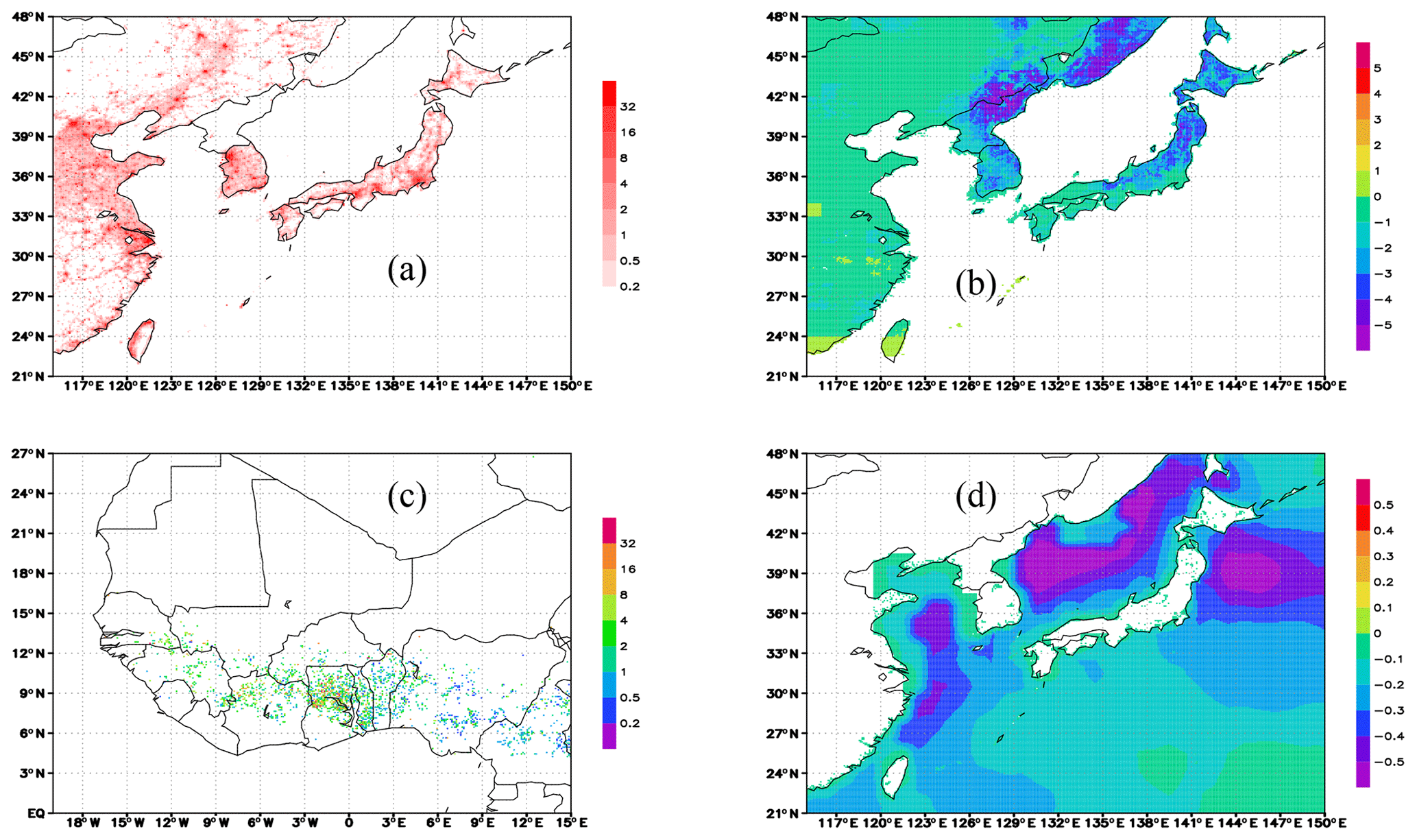
Figure 1Examples of prior CO2 fluxes (units gC m−2 d−1). (a) Emissions from fossil fuel burning by ODIAC (January 2011). (b) Fluxes from the terrestrial biosphere by the optimized VISIT model (day 160; 9 June 2011). (c) Emissions from biomass burning by GFAS in Africa (10 January 2011). (d) Fluxes due to the ocean–atmosphere exchange by the OTTM assimilation model (January 2011).
3.1 Emissions from fossil fuel
For the fossil fuel CO2 emissions (emissions due to fossil fuel combustion and cement manufacturing), we used the ODIAC data product (Oda and Maksyutov, 2011, 2015; Oda et al., 2018) at a resolution on monthly basis. The 2016 version of the ODIAC data product (ODIAC2016; Oda et al., 2018) is based on global and national emission estimates and monthly estimates made by the Carbon Dioxide Information Analysis Center (CDIAC; Boden et al., 2016; Andres et al., 2011). For spatial disaggregation, it uses the emission data for power plant emissions by the CARbon Monitoring for Action (CARMA) database (Wheeler and Ummel, 2008), while the rest of the national total emissions on land were distributed using spatial patterns provided by nighttime lights data collected by the Defence Meteorological Satellite Program (DMSP) satellites (Elvidge et al., 1999). The ODIAC fluxes were aggregated to a 0.1∘ resolution from the high-resolution ODIAC data (1×1 km). The ODIAC emission product is suitable for this kind of study because the global total emission is constrained by updated estimates, while providing a high-resolution emission estimate. Thus, it can be applied to carbon budget problems across different scales.
3.2 Terrestrial biosphere fluxes
CO2 fluxes by the terrestrial biosphere at a resolution of 0.1∘ were constructed using a vegetation mosaic approach, combining the vegetation map data by the Synergetic Land Cover Product (SYNMAP) data set (Jung et al., 2006), available at a 30 arcsec resolution, with terrestrial biospheric CO2 exchanges simulated by the optimized VISIT model (Saito et al., 2014) for each vegetation type in every 0.5∘ grid at a daily time step. The area fraction of each vegetation type is derived from SYNMAP data for each 0.1∘ grid. The CO2 net ecosystem exchange (NEE) fluxes on a 0.1∘ grid were prepared by combining the vegetation-type-specific fluxes with vegetation area fraction data on a 0.1∘ grid. By averaging the daily flux data for the period of 2000–2005, the flux climatology was derived for use in the recent years (after 2010) when the VISIT model simulation based on JRA-25–JCDAS reanalysis data was not available. Although the use of climatology in the place of original fluxes degrades the prior, the posterior fluxes show significant departures from prior, thus reducing the impact of missing the prior variations. The diurnal cycle was not resolved, as it requires one to also produce the gross primary production and ecosystem respiration. To estimate the effect of excluding the diurnal cycle in the prior fluxes for our selected time of sampling the observations, we compared CO2 concentrations simulated with diurnally varying fluxes at an hourly time step with those made with daily mean fluxes produced by the Simple Biosphere (SiB) model for 2002–2003 (Denning et al, 1996), as used in the Transcom continuous intercomparison (Law et al, 2008). The results show that, for background monitoring sites, the difference is not significant (below 0.1 parts per million – ppm), similar to the result by Denning et al. (1996). For continental sites, the difference between the two simulations was combined into four seasonal values, and the data for the season with the largest difference are shown in Fig. A1. Positive bias by simulation with daily constant flux, with respect to diurnally varying fluxes, is of the order of 0.5 to 1 ppm, and it is larger during the middle of the growing season. Inclusion of the diurnally varying fluxes in the place of the daily mean has the potential to change the seasonality of posterior fluxes by inversion in a favourable direction, as there are regions where flux seasonality is somewhat stronger than expected (Sect. 5.2).
3.3 Emissions from biomass burning
Daily biomass burning CO2 emissions by the Global Fire Assimilation System (GFAS) data set rely on assimilating fire radiative power (FRP) observations from the Moderate Resolution Imaging Spectroradiometer (MODIS) instruments on board the Terra and Aqua satellites (Kaiser et al., 2012). The fire emissions at a 0.1∘ resolution are calculated from FRP with land-cover-specific conversion factors compiled from a literature survey. The GFAS system adds corrections for observation gaps in the observations and filters spurious FRP observations of volcanoes, gas flares, and other sources. The fluxes are inputted to the model at the surface, which may lead to an underestimation of the injection height for strong burning events and the occasional overestimation of biomass burning signals simulated at surface stations.
3.4 Oceanic exchange flux
The air–sea CO2 flux component for the flux inversion used an optimized estimate of oceanic CO2 fluxes by Valsala and Maksyutov (2010). The data set was constructed with a variational assimilation of the observed partial pressure of surface ocean CO2 (pCO2), available in Takahashi et al. (2017) database, into the OTTM (Valsala et al., 2008), coupled with a simple one-component ecosystem model. The assimilation consists of a variational optimization method that minimizes the model observation differences of the surface ocean dissolved inorganic carbon (DIC or pCO2) within the 2-month time window. The OTTM model fluxes produced on a grid at monthly time step were interpolated to a grid, taking into account the land fraction map derived from the 1 km resolution MODIS land cover product.
3.5 Flux uncertainties for land and ocean
CO2 flux uncertainties are needed for both land and ocean regions. Climatological, monthly varying flux uncertainties for land were set to 20 % of the MODIS gross primary productivity (GPP) product (MOD17A2), available on a 0.05∘ grid at a monthly resolution (Running et al., 2004). Oceanic flux uncertainties were based on the sum of the standard deviation of the OTTM assimilated flux from the climatology by Takahashi et al. (2009) and the monthly variance of the interannually varying OTTM fluxes (Valsala and Maksyutov, 2010), with a minimum value of 0.02 gC m−2 d−1, in the same way as in the lower spatial resolution inverse model by Maksyutov et al. (2013). Oceanic flux uncertainties were first estimated on a resolution at a monthly time step and then interpolated to a grid, with the same procedure as for the oceanic fluxes.
3.6 Atmospheric CO2 observations
We used CO2 observation data distributed as the Observation Package–CO2 (ObsPack–CO2) GLOBALVIEWplus v2.1 (Cooperative Global Atmospheric Data Integration Project, 2016). The data from the flask sites were used as an average concentration for a pair of flasks. Afternoon (15:00 to 16:00 LT – local time) average concentrations were used for continuous observations over land and for remote background observation sites. For the continuous mountain top observations, we used early morning observations (05:00 to 06:00 LT). The geographical local time was used, as defined by the universal coordinated time (UTC), with a longitude-dependent offset. The list of the observation locations with the ObsPack site ID, site names, data providers, and data references appears in Table A1, accompanied by a site map in Fig. A2. The aircraft observational data collected by the NOAA aircraft programme at Briggsdale, Colorado (CAR), Cape May, New Jersey (CMA), Dahlen, North Dakota (DND), Homer, Illinois (HIL), Portsmouth, New Hampshire (NHA), Poker Flats, Alaska (PFA), Rarotonga, Cook Islands (RTA), Charleston, South Carolina (SCA), Sinton, Texas (TGC; Sweeney et al., 2015), and also by the Comprehensive Observation Network for TRace gases by AIrLiner (CONTRAIL) project over the western Pacific (CON; Machida et al., 2008) were grouped into averages for each 1 km altitude bin, with the altitude counted from sea level. Within the 1 km altitude range, the average value of both concentration and the altitude was taken. Aircraft observations were not assimilated, as they were only intended for use in the validation of the results.
4.1 Flux optimization problem
The inverse problem of atmospheric transport is formulated by Enting (2002) as finding the surface fluxes that minimize the misfit between the transport model simulation and the vector of observations y, where yf is the forward simulation without the surface fluxes, xp is the known prior flux, x is the unknown flux correction, and H represents the transport model. The equation has to be solved for the unknown flux correction x, and x is solved for at the transport model grid scale (Kaminski et al., 2001). By introducing the residual misfit vector , the problem can be formulated as minimizing a norm of difference () weighted by the data uncertainties. As the observation data alone are not sufficient to uniquely define the solution x, an additional regularization is required. By introducing additional constraints on the amplitude and smoothness of the solution, the inverse modelling problem is formulated (Tarantola, 2005) as solving for the optimal value of the vector x at the minimum of a cost function J(x) as follows:
where x is the optimized flux, R is the covariance matrix for observations, and B is the covariance matrix for surface fluxes. By introducing a decomposition of B as (construction of matrix L explained in detail in Sect. 4.2) and a variable substitution , the second term in Eq. (1) is simplified. At the same time, by assuming that R can be decomposed into , where σ is a vector of data uncertainties, and introducing expressions and , the new form of Eq. (1) is introduced as follows:
The solution minimizing J(z) can be obtained by forcing the derivative to be zero, which results in the following:
An optimal solution z at the minimum of the cost function J(z) is found iteratively with the Broyden–Fletcher–Goldfarb–Shanno (BFGS) algorithm (Broyden, 1969; Nocedal, 1980), as implemented by Gilbert and Lemarechal (1989). The method requires the ability to accurately estimate the cost function J(z) and its gradient and has modest memory storage demands. Given the solution z, the flux correction vector x is then found by reversing the variable substitution as .
The convergence of the solution may be affected by the accuracy of the adjoint. The result of the duality test, defined as the norm of the difference between the NIES-TM–FLEXPART forward and adjoint modes estimated as (), was found to be of the order of 10−9, while for the Lagrangian component based on the receptor sensitivity matrices prepared with FLEXPART, it is about 10−15 when calculated in double precision (same as in Belikov et al., 2016). The formulation of the minimization problem, as presented by Eq. (2), is convenient for the derivation of the flux uncertainties, as it is possible to solve Eq. (3) via the truncated singular value decomposition (SVD) and estimate the regional flux uncertainties based on the derived singular vectors (Meirink et al., 2008). Alternatively, as mentioned by Fisher and Courtier (1995), it is also possible to use the flux increments derived at each iteration of the BFGS algorithm in the place of the singular vectors. Although we did not use SVD to construct the posterior covariances in this study, we tested the solving of the optimization problem with SVD. We derived the SVD of ATA using a computer code by Wu and Simon (2000), which implements an algorithm proposed by Lanczos (1950), and confirmed that this approach yields practically the same solution as the one obtained with the BFGS algorithm. The Lanczos (1950) algorithm is a commonly used SVD technique, applied in the case of a large, sparse matrix or a linear operator, when it is impractical to make direct use of the SVD of A. A truncated SVD of A is given by the expression A≈UΣVT, where Σ is the diagonal matrix of n singular values, while U and V are the matrices of left and right singular vectors. Variable substitutions, including the following:
transform z into a space of singular vectors s and reduce Eq. (3) to , resulting in the following solution:
which is evaluated directly, as Σ is diagonal. In case of having only n largest singular values, the elements of the solution s are given by for all i≤n. Once the solution (Eq. 5) is found, it is taken back to the space of the dimensional fluxes z by applying variable substitutions (Eq. 4). For fluxes, we have , z=VTs, and d=UTb; thus, the solution is provided by the following:
Another variant of the SVD approach may be more memory efficient in the case of a very large dimension of a flux vector. Then, applying SVD to AAT instead of ATA can save some memory, as in a representer method (Bennett, 1992). It gives the same solution as the SVD of ATA and uses less intermediate memory storage when the dimension of the observation vector y is lower compared to that of the flux vector x.
The forward and adjoint mode simulations with the transport model needed to implement the iterative optimization are composed of several steps, as follows:
-
Running the Lagrangian model FLEXPART to produce the source–receptor sensitivity matrices. For each observation event, a backward transport simulation with the FLEXPART model is implemented to produce the surface flux footprints, at a latitude–longitude resolution, and the 3-D concentration field footprint, taken at the end of the backward simulation run (ending at the coupling time of 00:00 Greenwich mean time – GMT). The coupling time is set to be within 2 to 3 d before the observation event. The surface flux sensitivity data are recorded in the unit of ppm (gC m−2 d. The flux footprints are saved at a daily or hourly time step, depending on available surface fluxes.
-
Running the coupled transport model forward, which includes the following:
- a.
Running the 3-D Eulerian model NIES-TM from the 3-D initial concentration field, with the prescribed surface fluxes. This includes sampling the 3-D field at model coupling times for each observation, according to 3-D concentration field footprints calculated at the first step by FLEXPART. NIES-TM reads the same 0.1∘ fluxes as the Lagrangian transport model and remaps them onto its grid before including them in the simulation. For each observation event, the fluxes used in Eulerian and Lagrangian components are separated by the coupling time, so that there is no double counting of fluxes for the same date in the coupled model simulation.
- b.
Using the two-dimensional (2-D) surface flux footprints prepared with the Lagrangian model to calculate the surface flux contribution to the simulated concentrations for the last 3 d.
- c.
Combining the concentration contributions produced by Eulerian (a) and Lagrangian (b) components to give the total simulated concentration.
- a.
-
In the inverse modelling, the transport model is run in the following three modes:
- a.
The forward model is first run with prescribed prior fluxes, starting from the 3-D initial CO2 concentration field, to calculate the residual misfit (difference between the observation and the model simulation).
- b.
At the inverse modelling/optimization step, only the flux corrections are propagated in the forward model runs, which are optimized to minimize the observation–model misfit. The prescribed prior fluxes are not used (switched off) at this step. The model starts from a zero 3-D initial concentration field and runs forward, with flux corrections updated by the optimization algorithm at every iteration, to produce simulated concentrations. Corrections to the 3-D initial concentration field are not estimated and, thus, not included in the control vector. Instead, the model is given a spin-up period of 3 months before the target flux estimation period to adjust the simulated concentration to the observations.
- c.
In the adjoint mode, the adjoint mode atmospheric transport is simulated backward in time, starting from the vector of residuals to produce a gradient of the cost function (defined as Eq. 1) with respect to the surface fluxes. Given the gradient, the optimization algorithm provides the new flux corrections field. For convenience, the transport model and its adjoint are implemented as procedures suitable for direct communication mode.
- a.
Step 1 is carried out in the same way as in other versions of the coupled transport model (Zhuravlev et al., 2013; Shirai et al., 2017). In steps 2 and 3, the procedure of running the forward and adjoint model is organized differently. At the beginning of the transport model runs, all the data prepared by the Lagrangian model are stored in the computer memory in order to save on the time required for reading and re-sorting the data at each iteration. The fraction of the CPU time spent on running the Eulerian component of the coupled transport model is 82 %, with 1 % used on the Lagrangian component and 17 % used for covariance.
To create the initial concentration field, we used a 3-D snapshot of the CO2 concentration for the same day from a simulation of the previous year, which is already optimized (usually 1 October or 1 January). When such a simulation was not available, we took a snapshot from an available year and corrected it globally for the concentration difference between these years, using the NOAA monthly mean data for the South Pole as representative for the global mean concentration. When the optimized fields are not available, the output of the multiyear spin-up simulation is used, with the same adjustment to the South Pole observations.
4.2 Implementation of covariance matrices L and B
We optimized surface flux fields separately for two sets of fluxes in every grid globally, for land and ocean regions, following the approaches by Meirink et al. (2008) and Basu et al. (2013), who suggested optimizing for global surface flux fields separately for each optimized flux category. Separating the total flux into independent flux categories, each with its own flux uncertainty pattern, results in using homogenous spatial covariance matrices, significantly simplifying the coding of the matrix B. The matrix B can be given as the product of a diagonal matrix of flux uncertainties and a matrix with 1.0 as diagonal elements, while non-diagonal elements are exponentially declining with the squared distance between grid points (Meirink et al., 2008). In practice, an extra scaling of the uncertainty is needed to balance the constraint on fluxes with the data uncertainty, which also impacts the regional flux uncertainties. Several empirical methods are in use, where the tuning parameters are a horizontal scale (Meirink et al., 2008) and an uncertainty multiplier (Chevallier et al., 2005; Rödenbeck, 2005). In our B matrix design, we follow Meirink et al. (2008) in representing B matrix as the multiple of the non-dimensional covariance matrix C and the diagonal matrix of the flux uncertainty D as . C matrix is commonly implemented as a band matrix, with non-diagonal elements declining as , with the distance x between the grid cells as in 2-D spline algorithms (Wahba and Wendelberger, 1980). Multiplication by the matrix C becomes computationally costly at a high spatial resolution in cases where the correlation distance l is much larger than the size of the model grid. The correlation distance used here is 500 km for land and ocean and 2 weeks in time. The rationale of applying a correlation distance of 500 km in the case of a regional inversion over the continental USA with a model grid size of 40 km was discussed by Schuh et al. (2010). In that case, the use of an implicit diffusion with a directional splitting to approximate the Gaussian shape appears to be computationally more efficient than the direct application of the Gaussian-shaped smoothing function, as the number of floating-point operations per grid point does not grow with the ratio of the correlation distance l to the grid size. The covariance matrix based on the diffusion operator is popular in many ocean data assimilation systems, as it is a convenient way to deal with coastlines (e.g. Derber and Rosati, 1989; Weaver and Courtier, 2001).
The idea of using the solution of the diffusion equation instead of multiplying a vector by the covariance matrix can be presented briefly in a 1-D case. Consider a discrete problem of multiplying a vector representing a function g(λ) on a grid with spacing Δλ by a symmetric matrix which has diagonal elements equal to one, and non-diagonal ones declining as , with a distance of i points from the diagonal, where d is covariance length. Its continuous analogue is an application of a Gaussian-shaped smoother in the form to a function g(λ) as follows:
where the smoothing window size l should be several times larger than d. The expression in Eq. (7) looks exactly like the solution of a 1-D diffusion equation, as follows:
where D is the diffusivity. The solution of Eq. (8) is given by , where p2=2DΔt, g(λ) is the initial distribution, and Δt is the time step (Crank, 1975). Based on this equivalence, instead of multiplying a vector by the covariance matrix, we solve the discrete form of Eq. (8) by the backward-in-time, central-in-space implicit method.
Applying the diffusion operator for the covariance matrix helps to achieve the spatial homogeneity between polar and equatorial regions, as diffusion produces a theoretically uniform effect on flux fields – regardless of the polar singularity. The diffusion operator works as a low-pass filter, selectively suppressing all the wavelengths shorter than the covariance length scale. As we need to construct the covariance matrix B in the form , we choose to construct L first and then derive its transpose LT. The factorization of L is given by , where Lt is the 1-D covariance matrix for the time dimension, and ⊗ is a Kronecker product. We approximate the 2-D covariance Lxy by splitting it into two dimensions, namely latitude and longitude as in Chua and Bennett (2001), and apply several iterations of this process. The horizontal covariance Lxy is implemented in N=3 iterations of 1-D diffusion so that , where Lx and Ly are the covariance operators for longitude and latitude directions, respectively, while uF is the diagonal matrix of flux uncertainty for each grid cell and each flux category (land and ocean), and m is the diagonal matrix of a map factor, which is introduced to scale the contributions to the cost function by model grid area, with diagonal elements given by (where θ is latitude).
This design of the covariance operator helps to preserve the high-resolution structure of the resultant flux corrections, given by , as it can be factored into a multiple of uncertainty uF and a scaling factor as . While the scaling factor S is smoothed with a covariance length of 500 km, the original structure of the spatial heterogeneity of surface flux uncertainty uF is still preserved at the original high resolution in the optimized flux corrections x.
The adjoint operators and are derived by applying the adjoint code compiler Tapenade (Hascoet and Pascual, 2013) to the Fortran code of modules that approximate the operators Lx and Ly by implicit diffusion. Lt and its transpose are of lower dimensions and are designed, as in Meirink et al. (2008), by deriving the square root of the Gaussian-shaped time covariance matrix with direct SVD (Press et al., 1992).
A notable merit of the algorithm is that it minimizes the use of the computer's memory, avoiding allocations of the memory space that are larger than several times the dimension of the observation and flux vectors, making it suitable for ingesting large amounts of surface and space-based observations. It should be mentioned that the computer memory demand for accommodating the surface flux sensitivity matrices for massive space-based observations can be a limiting factor, as discussed by Miller et al. (2020).
4.3 Inversion set-up
The combination of the coupled transport model NIES-TM–FLEXPART (as described in Sect. 2) with the variational optimization algorithm (Sect. 4.1 and 4.2) constitutes the inverse modelling system NIES-TM–FLEXPART-VAR (NTFVAR or NIES-TM–FLEXPART-variational). We tested the inversion algorithm presented in previous sections with the problem of finding the best fit to the CO2 observations provided by the ObsPack data set by optimizing the corrections to the land and ocean fluxes. By design, our inverse modelling system produced smoothed fields of scaling factors that are multiplied by the fine-resolution flux uncertainty fields to give flux corrections. We derived the surface CO2 flux corrections at a 0.1∘ resolution and biweekly time step. Our purpose is to demonstrate that we can optimize fluxes to improve the fit to the observations, using an iterative optimization procedure based on a high-resolution coupled transport model and its adjoint. Our report is limited to the technical development towards achieving the capability of estimating anthropogenic CO2 emissions based on atmospheric observations, and we do not elaborate on the impact of simulating the tracer transport at a high resolution on the quality of the optimized natural fluxes, which requires an additional study. The flux optimization was applied to a short time window of 18 months for each optimized year, and the simulation starts on 1 October, 3 months ahead of the target year. A spin-up period of 3 months is given to let the inversion adjust the modelled concentration to the observations so that a balance is achieved between fluxes, concentrations, and concentration trends. The simulation is continued until reaching the limit of 45 cost function gradient calls, and by that time, the M1QN3 procedure by Gilbert and Lamarechal (1989) is able to complete 30 iterations. Figure A3 presents the cost function reduction in the case of optimizing fluxes for 2011 and completing 61 gradient calls. The cost function reduction declines nearly exponentially, by almost 3 times, for each 10 gradient calls completed. The relative improvement between 41 and 61 gradient calls is 1.5 % of the total reduction from the first to the 61 gradient calls. We optimized fluxes for 3 years from 2010 to 2012 and analysed the simulated concentration fit at the observation sites. The average root mean squared misfits (RMSE) between the optimized concentrations and the observations are compared with a forward simulation with prior fluxes and optimized simulation. For evaluation, we used statistics of the optimized simulations by the operational NOAA's CarbonTracker inverse modelling system (ObsPack_co2_1_CARBONTRACKER_CT2017_2018-05-02; Peters et al., 2007).
5.1 Analysis of the posterior model fit to the observations
We compared the results of the forward simulation with prior and optimized fluxes with the processed observations for ground observation sites, as shown in Table A1, and airborne vertical profiles were used for an independent validation (Table A2). Figure 2 shows the observations with forward (prior) and optimized simulations at Barrow (BRW), Jungfraujoch (JFJ), Wisconsin (LEF), Pallas (PAL), Yonagunijima (YON), and Syowa (SYO). The optimization yielded improved seasonal variations in the simulated concentration, including the phase and the amplitude at most sites. At SYO, we found synoptic scale variations with an amplitude of the order of few tenths of a part per million that were, to a large extent, captured by the model. Plots for BRW and JFJ show the ability of the inversion to correct the seasonal cycle, while the difference between model and observations in the Southern Hemisphere (SYO) is contributed by the interannual variations in the carbon cycle. The model–observation mismatch (RMSE) for surface sites included in the ObsPack is presented in Fig. 3 for forward and optimized simulation and mean bias for optimized data. The model was able to reduce the model to observation mismatch for most background sites where the seasonal cycle is affected mostly by natural terrestrial and oceanic fluxes, while the average reduction in the mismatch from forward to optimized simulation is 14 %, which is defined as the mean ratio of the optimized mismatch to the forward mismatch taken for each site. The reason for the relatively small reduction is the addition of climatological flux corrections to the prior simulation, estimated by inverse modelling of 2 years of data, namely 2009 and 2010. As a result, the inversion starts from the initial flux distributions already adjusted to fit the seasonal cycle of the observed concentration. The correction for the difference in the global concentration trend between years is not made; thus, there are visible differences between prior and optimized simulations in the southern hemispheric background sites. At most of the Antarctic sites, the mean posterior (after optimization) mismatch (reported as RMSE) is of the order of 0.2 ppm. Over the land, closer to anthropogenic sources, there is a less relative reduction in the mismatch on an annual mean scale. One of the reasons for seeing little improvement is that fossil CO2 emissions are kept fixed and only the natural fluxes are optimized (while the strong signal from fossil emission is not affected by flux corrections). Another possible contributor to the large mismatch over land is the neglect of the diurnal cycle, under the assumption of using only observations at well-mixed conditions, and also the limited ability of the low-resolution reanalysis data set to capture frontal processes in the extratropical continental atmosphere, as discussed by Parazzoo et al. (2011). The mean mismatch was reduced from 2.60 to 2.42 ppm by the flux optimization, while the mean mismatch to the uncertainty ratio decreases after optimization by 19 % from 0.94 to 0.78. The mean correlation between modelled and observed data improves from r2=0.43 (r2 – coefficient of determination) for the simulation driven by prior fluxes to r2=0.59 for the optimized simulation. To remove the effect of the interannual CO2 growth on CO2 variabilities, the mean growth trend was subtracted from the data before estimating the r2.
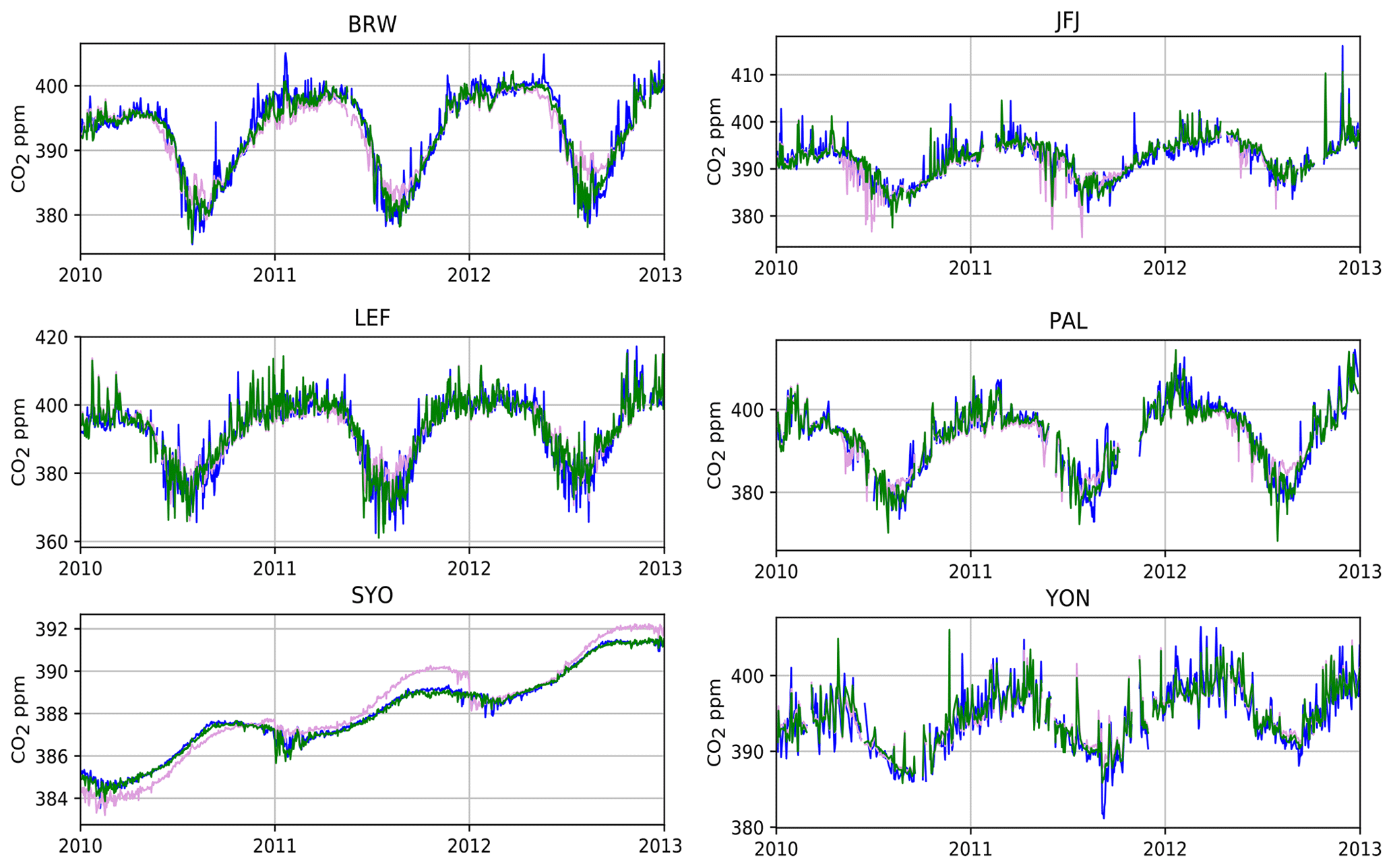
Figure 2Time series of simulated and observed concentrations (blue – observed; plum – forward (unoptimized); green – optimized) at Barrow (BRW), Jungfraujoch (JFJ), Wisconsin (LEF), Pallas (PAL), Syowa (SYO), and Yonagunijima (YON).
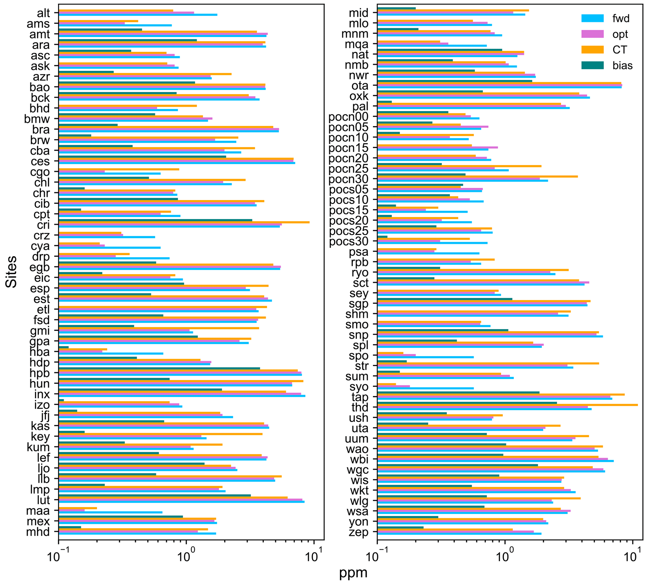
Figure 3Root mean square difference between model and observations and absolute bias in 2010–2012 for (surface) sites included in inversion (blue – prior; pink – optimized; orange – CT 2017; green – absolute value of mean difference (bias) for optimized).
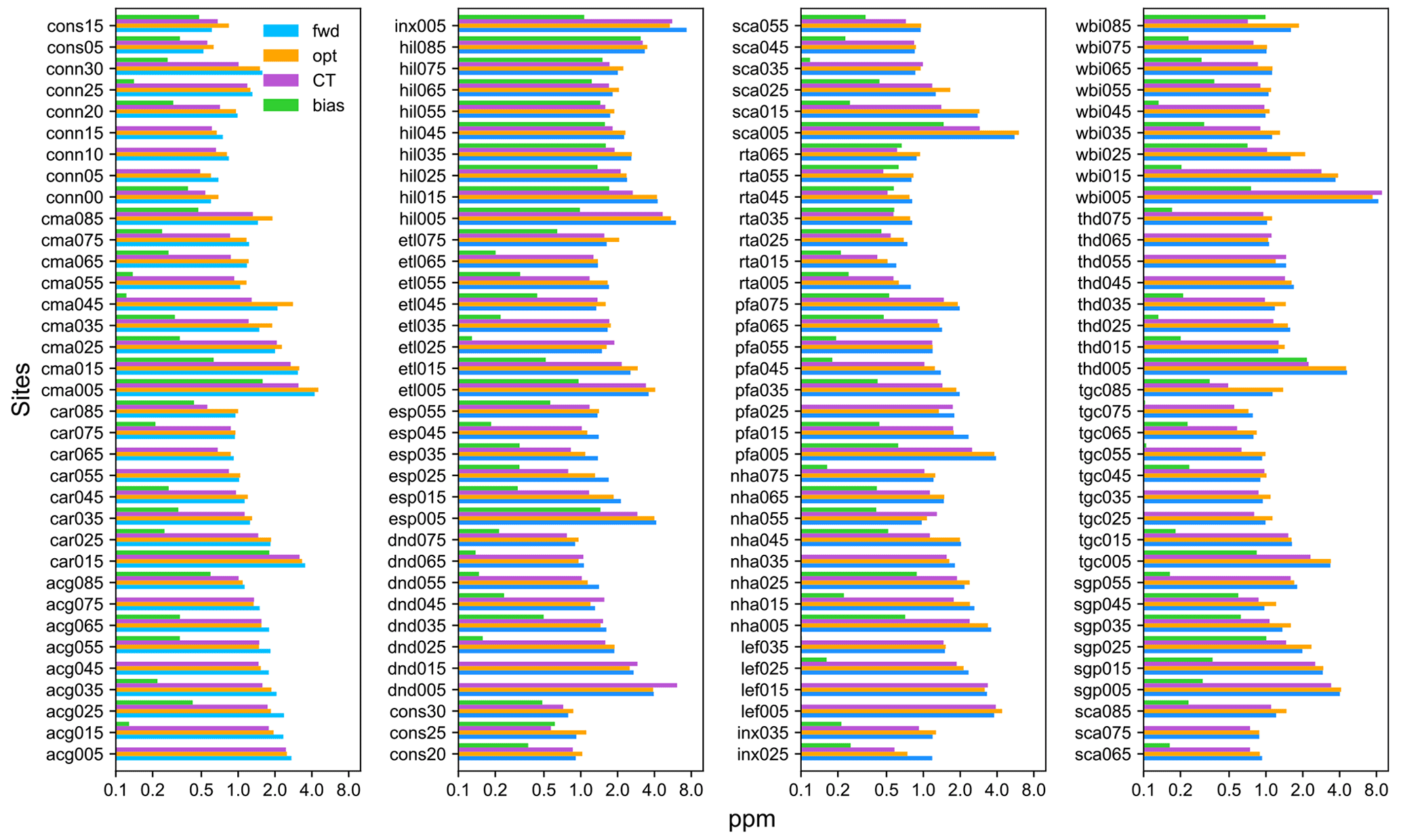
Figure 4Root mean square difference between model and observations and absolute bias in 2010–2012 for aircraft sites not included in inversion (blue – prior; orange – optimized; magenta – CT 2017; green – absolute value of mean difference (bias) for optimized).
Figure 3 also shows, for the purpose of comparison, the statistics of the average misfit for the optimized simulation by CarbonTracker for the same period and same monitoring stations. The comparison is useful for understanding the strengths and weaknesses of the inversion system presented here. Over the background monitoring sites, the high-resolution model does not show any advantage over CarbonTracker in terms of the fit between the optimized model simulation and observations, which may indicate a better performance by the Eulerian model, TM5, used in CarbonTracker. On the other hand, several sites where the high-resolution model shows better fits to observations over CarbonTracker are located inland or near the coast, closer to anthropogenic and biogenic sources. A smaller misfit was achieved by the high-resolution model at Key Biscayne (KEY), Baring Head (BHD), Mariana Islands (GMI), and Cape Kumukahi (KUM), among others, which can be attributed to coastal/island locations, while there is little or no advantage at mountain sites like Mauna Loa (MLO) or Jungfraujoch (JFJ). This result may be influenced by differences in the model physics between NIES-TM–FLEXPART and TM5 in the lower troposphere, near the top of the boundary layer, and in shallow cumuli. The mismatch (RMSE) between our optimized model and observations for the 102 sites used in the inversion is only 4 % lower on average than that by CarbonTracker. It is not yet clear if there is a systematic advantage of one or the other system in any particular site category, other than for coastal/island sites mentioned above. For the average misfit comparison, all data, both assimilated and not assimilated, are included for sites shown in Fig. 3. The results for Cape Grim (CGO) were not counted due to the use of different data sets, as our system used only the NOAA flask data, which underwent background selection (by wind direction) at the time of sampling.
As an independent validation, a comparison of the unoptimized and optimized simulation to the vertical profile data is shown in Fig. 4. For each vertical profile site, the observations were grouped by altitude, at a 1 km interval. The altitude code (e.g. 005, 015, 025, 035, …) to be added to the site identifier was constructed as the altitude of the midlevel multiplied by 10. The observations at PFA (Poker Flat, Alaska) between the surface and 1 km were grouped as PFA005 (mid-altitude 0.5 km), while those in the 5 to 6 km range were designated as PFA055 (mid-altitude 5.5 km). As for the optimized surface data in Fig. 3, we show the RMSE for forward simulation with prior fluxes, optimized simulation, and CarbonTracker and mean bias for optimized data. CarbonTracker shows a better fit at most of the altitude ranges, except for the lowest 1 km where the results shown by the two systems were similar. Concurrently, the mean correlation between modelled and observed data did not improve from the prior (r2=0.70) to the optimized simulation (r2=0.63), while the mean RMSE declined a little from 1.86 to 1.85 ppm. The comparison to CarbonTracker (CT 2017), with a mean RMSE of 1.53 ppm, suggests that the free tropospheric performance of our system can be improved by implementing a more detailed vertical mixing processes in the Lagrangian and Eulerian component models.
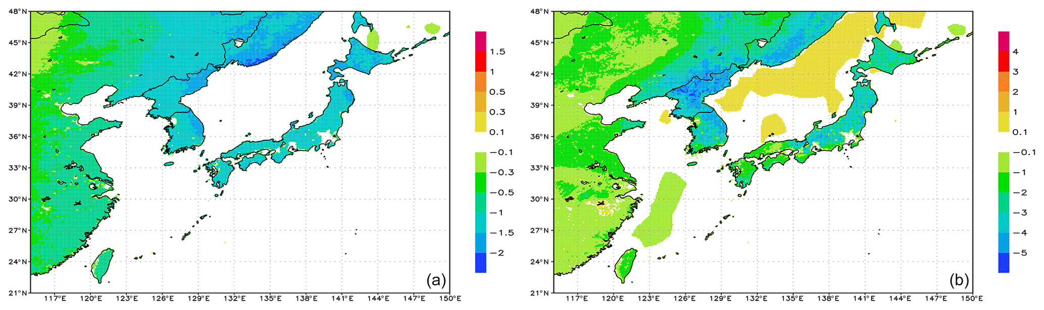
Figure 5Optimized flux correction (a) and posterior flux (b) maps for August 2011 (units gC m−2 d−1; fossil emissions excluded).
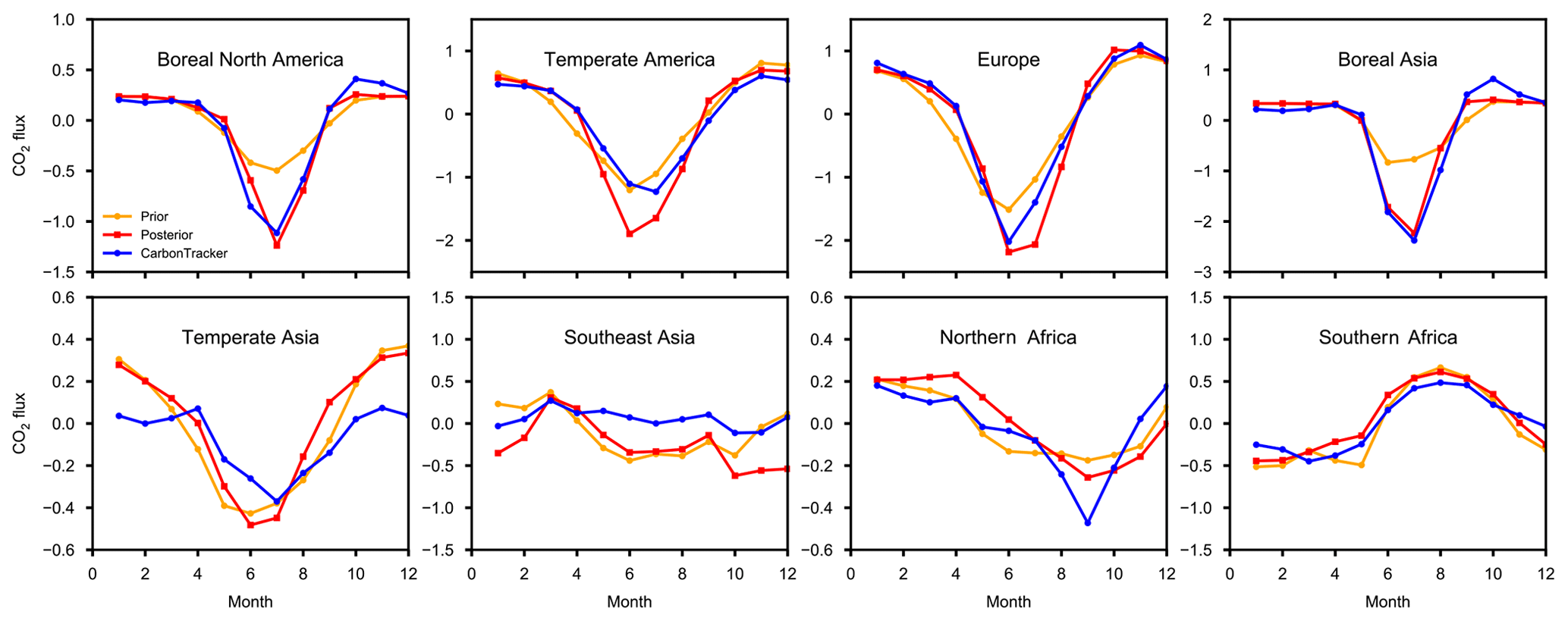
Figure 6Monthly mean prior, optimized, and CarbonTracker fluxes (fossil emissions excluded) averaged for 2010–2012 for selected Transcom-3 regions (units gC m−2 d−1).
5.2 Comparison of prior and posterior fluxes
As mentioned in Sect. 4.2, the flux corrections estimated by the inverse model showed fine-scale features, despite using large covariance lengths, because those were made of the high-resolution data uncertainty multiplied by the smooth fields of scaling factor and estimated separately for each of the optimized flux categories, namely land biosphere and ocean. Examples of the flux corrections and posterior fluxes (excluding fossil emissions) are presented in Fig. 5. The flux corrections and fluxes are shown in Fig. 5 for 1 month (August 2011) as an illustration, and they are not representative of a seasonal or climatological mean. The sign of the flux corrections changed from positive (source) in the eastern side (continental China) to negative (sink) over the Russian coast and Japanese islands, while the posterior fluxes appeared as a terrestrial sink all over the area. The flux adjustment was driven by the fit to nearby observations made over South Korea and Japan.
To illustrate the change in fluxes from prior to posterior estimates by the inversion at the scale of large aggregated regions, the monthly mean fluxes (excluding fossil emissions) averaged for 3 years (2010–2012) are plotted in Fig. 6 for eight selected Transcom regions (as defined by Gurney et al., 2002; see the map in Fig. A2). The plots include prior, optimized, and, for reference, optimized fluxes by CarbonTracker (CT 2017). For some regions, the posterior is close to the prior, which is often the case when there are too few observations in the region to drive the corrections to prior fluxes. Boreal North America (region 1), temperate North America (region 2), and Europe (region 11) are better constrained by observations, while Northern Africa (region 5), Southern Africa (region 6), temperate Asia (region 8), tropical Asia (region 9), and boreal Asia (region 7) are less constrained. The optimized flux is similar to the prior for Africa (regions 5 and 6), tropical Asia (region 9), and temperate Asia (region 8), while there is a substantial adjustment for boreal Asia (region 7), which seems to be adjusted to fit the observations outside the region. For both boreal regions, the prior flux seasonality appears weaker than in both posterior and CarbonTracker fluxes, which could indicate a problem with vegetation-type mapping in a higher resolution version of the prior flux model. For regions 1, 6, 7, and 11, the corrected fluxes are closer to CarbonTracker, and for temperate North America, temperate Asia, and Northern Africa, the amplitude of flux seasonality is estimated to be stronger, which can be caused by stronger vertical/horizontal mixing in the transport model as compared to the transport in CarbonTracker. A more detailed comparison with other inverse model results and independent estimates (e.g. by Jung et al., 2020) should be made after improving the inversion set-up, notably by improving the transport model meteorology, seasonality, and diurnal cycle in prior fluxes and the seasonality in prior flux uncertainties.
A grid-based CO2 flux inversion system that is suitable for the inverse estimation of the surface fluxes at a biweekly time step and a 0.1∘ spatial resolution was developed. To implement the high-resolution simulation capability, several developments were completed. High-resolution prior fluxes were prepared for the following three surface flux categories: fossil emissions by the ODIAC data set were based on the point source database and night lights, biomass burning emissions (GFAS) were based on MODIS observations of fire radiative power, and biosphere exchange was based on the mosaic representation of land cover and the process-based VISIT model simulation. A high-resolution atmospheric transport for a global set of observations was achieved by combining short-term simulations with the high-resolution Lagrangian model, FLEXPART, with a global 3-D simulation with the medium-resolution Eulerian model, NIES-TM. The use of variational optimization with a gradient-based method in the inversion helps to avoid the need for inverting large matrices with dimensions dictated by the number of optimized flux grids or the number of observations. Accordingly, the adjoint of the coupled transport model was developed to apply the variational optimization. A computationally efficient implementation of the flux error covariance operator is achieved by using an implicit diffusion algorithm. Overall, the presented algorithm demonstrated the feasibility of the high-resolution inverse modelling at the global scale, extending the capabilities achieved by regional high-resolution modelling approaches used for estimating the national greenhouse gas emissions for a comparison with the national greenhouse gas inventories. A comparison of the optimized simulation to the observations showed some improvements over the lower-resolution CarbonTracker model for some continental and coastal observation sites located closer to anthropogenic emissions and strong biospheric fluxes, but it also demonstrates the need for further improvement of the inverse modelling system components. Transport model errors can be reduced by improving the transport modelling algorithms in the Eulerian and Lagrangian models and using a combination of recent higher-resolution reanalysis data with high-resolution wind data simulations by regional models in the regions of interest. Our inverse modelling algorithm can be further improved by tuning the uncertainty scaling and spatial and temporal covariance distances. Prior fluxes can be improved by developing high-resolution, diurnally varying biospheric fluxes, developing a more detailed fossil emission inventory and updating the estimates of biomass burning and oceanic fluxes.
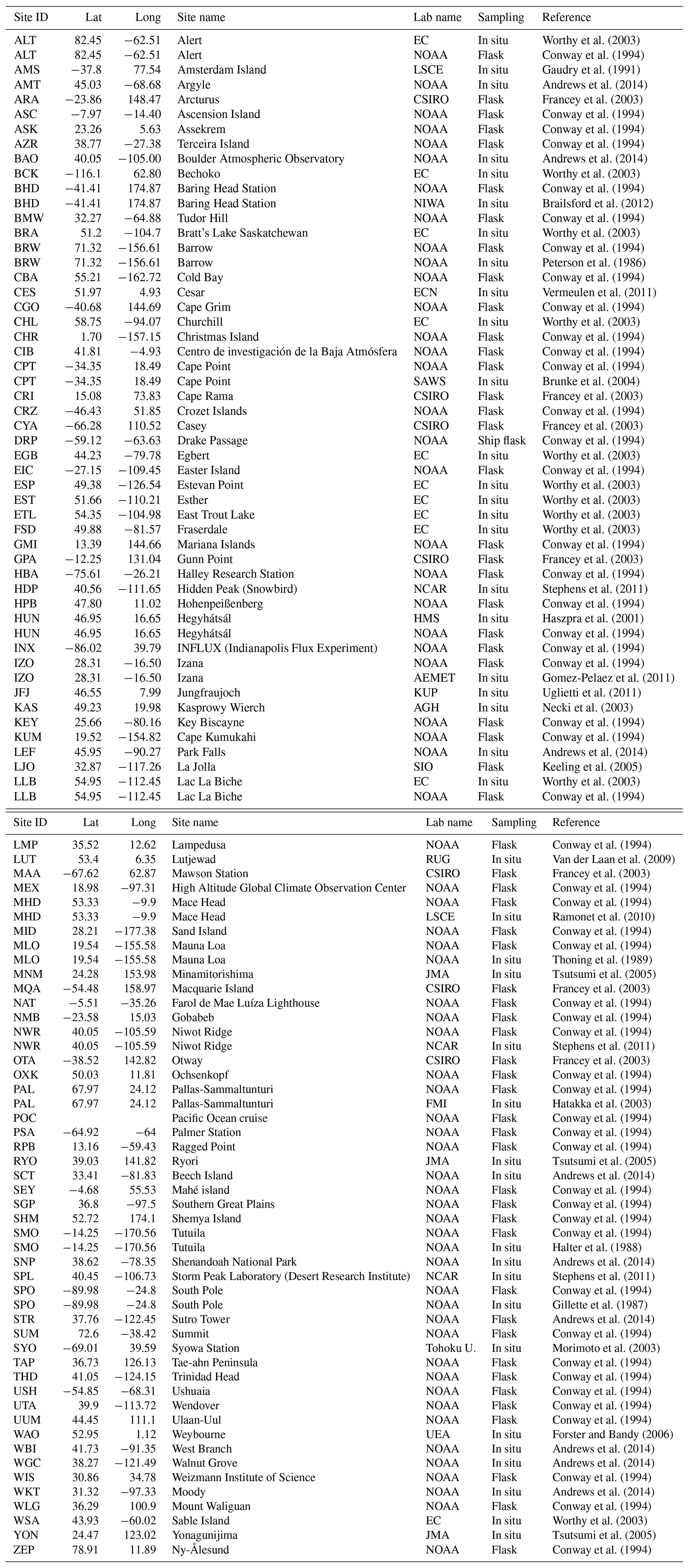
Table A2Validation sites. Aircraft data collected by NOAA and the Earth System Research Laboratory (ESRL; Sweeney et al., 2015) and NIES (Machida et al., 2008).
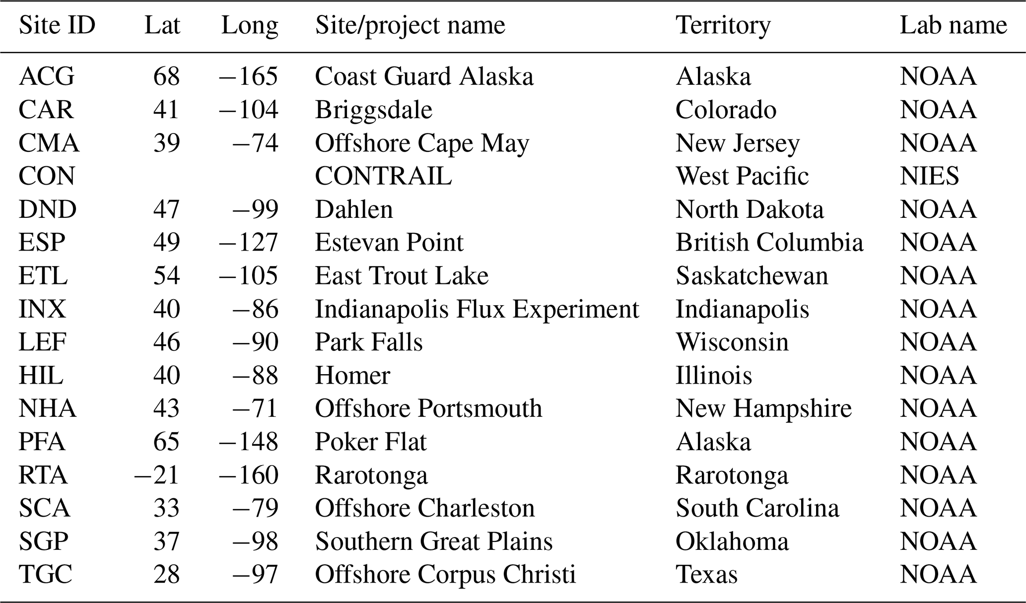
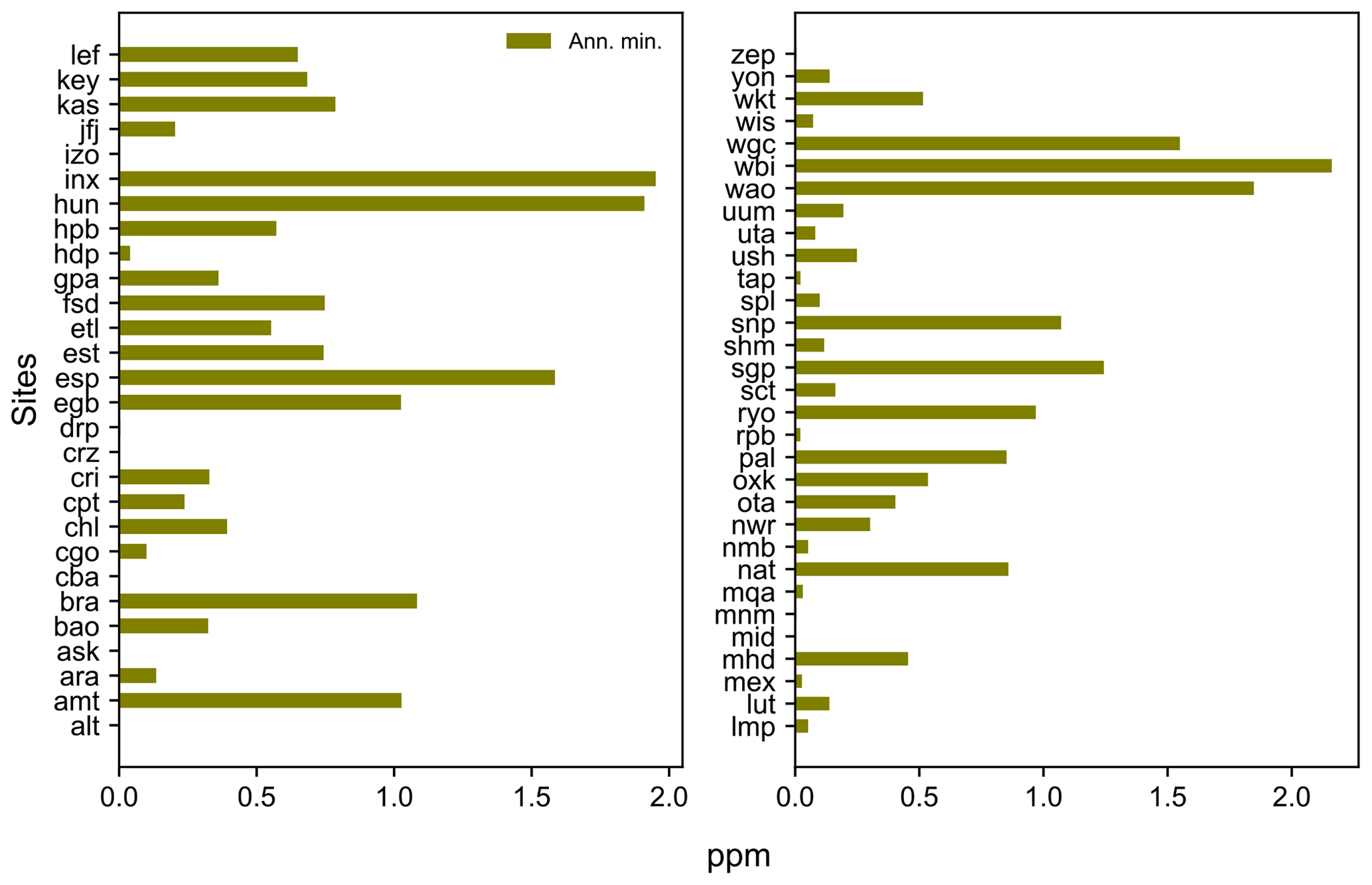
Figure A1Simulated diurnal cycle bias, showing the 3-month mean in the growing season (units in ppm).
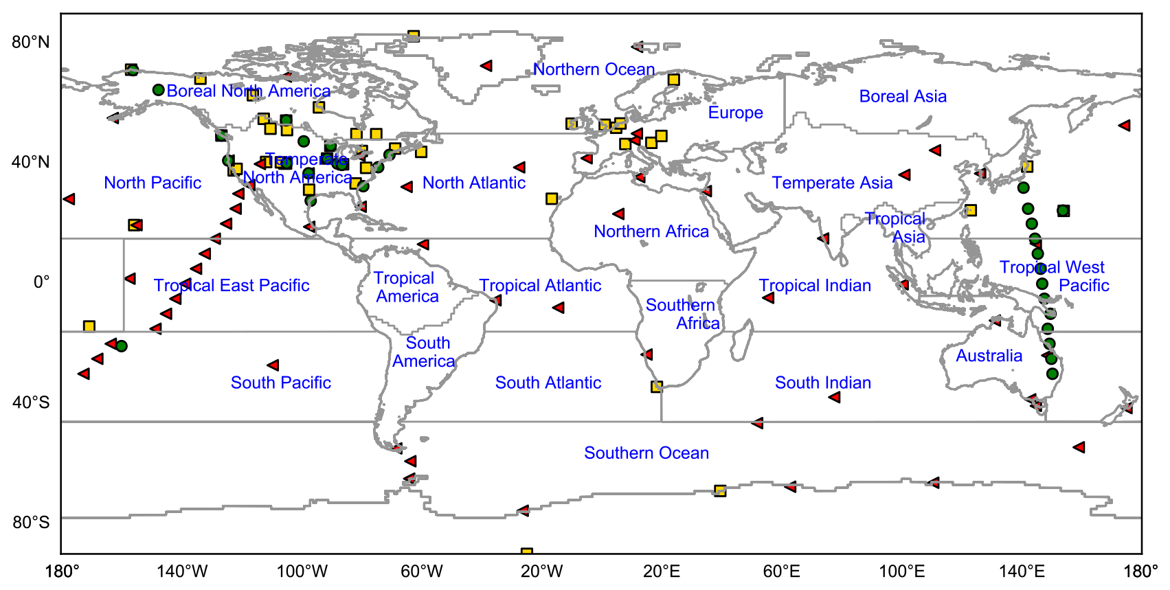
Figure A2A map of observation sites and Transcom regions (triangles – surface flask sites; squares – continuous; circles – aircraft) used in this study.

Figure A3Rate of cost function decline, with gradient calls for the extended year 2011 inversion, and reduction relative to 61 gradient calls.
The inverse model and forward transport model code can be made available to potential research collaborators upon reasonable request. The ObsPack data set is available from NOAA/ESRL (https://doi.org/10.15138/g3059z; Cooperative Global Atmospheric Data Integration Project, 2016). The ODIAC fossil fuel emission data set is available from the Global Environmental Database hosted by CGER/NIES (https://doi.org/10.17595/20170411.001; Oda and Maksyutov, 2015).
The supplement related to this article is available online at: https://doi.org/10.5194/acp-21-1245-2021-supplement.
SM developed the inverse and forward transport model algorithms and model codes, ran the model, analysed the results, and wrote the paper. TO developed the anthropogenic emission inventory, MS developed the biospheric flux data set, JK provided the biomass burning emission fluxes, and VV prepared the oceanic CO2 fluxes. RJ contributed to model testing and data preparation. DB contributed to the development of the NIES transport model, coupled model, and coupled adjoint. RZ and AG developed the Lagrangian response simulation system based on the FLEXPART model. AA, LC, ED, LH, TM, TN, MR, RL, CS, and DR contributed the observational data. All authors contributed to the development of the paper.
The authors declare that they have no conflict of interest.
The authors acknowledge the use of the computing resources at the National Institute for Environmental Studies (NIES) supercomputer facility and support from the GOSAT project, with project leaders Tatsuya Yokota and Tsuneo Matsunaga, the Ministry of the Environment (MOE) of Japan, an MRV grant to NIES, and grants from the Ministry of Education, Culture, Sports, Science and Technology (MEXT) of Japan for the GRENE and ArCS projects. The model development benefitted from fruitful discussions with Frederic Chevallier, David Baker, Peter Rayner, Aki Tsuruta, Fenjuan Wang, Prabir Patra, John Miller, Misa Ishizawa, Tomoko Shirai, and the members of the TRANSCOM project. Lorna Nayagam provided technical assistance to our model testing and data set developments. The authors appreciate the contribution of the NOAA CarbonTracker data provided by Andy Jacobson and colleagues. The ObsPack was compiled and distributed by NOAA/ESRL. The authors are grateful to the ObsPack data contributors at NOAA GMD, Environment and Climate Change Canada, and other institutions worldwide, including Tuula Aalto, Shuji Aoki, Gordon Brailsford, Marc L. Fischer, Grant Forster, Angel J. Gomez-Pelaez, Juha Hatakka, Arjan Hensen, Casper Labuschagne, Ralph Keeling, Paul Krummel, Markus Leuenberger, Andrew Manning, Kathryn McKain, Frank Meinhardt, Harro Meijer, Shinji Morimoto, Jaroslaw Necki, Paul Steele, Britton Stephens, Atsushi Takizawa, Pieter Tans, Kirk Thoning, and their colleagues.
This research has been supported by the GOSAT project at the National Institute for Environmental Studies.
This paper was edited by Christoph Gerbig and reviewed by two anonymous referees.
Agustí-Panareda, A., Diamantakis, M., Massart, S., Chevallier, F., Muñoz-Sabater, J., Barré, J., Curcoll, R., Engelen, R., Langerock, B., Law, R. M., Loh, Z., Morguí, J. A., Parrington, M., Peuch, V. H., Ramonet, M., Roehl, C., Vermeulen, A. T., Warneke, T., and Wunch, D.: Modelling CO2 weather – why horizontal resolution matters, Atmos. Chem. Phys., 19, 7347–7376, https://doi.org/10.5194/acp-19-7347-2019, 2019.
Andres, R., Gregg, J., Losey, L., Marland, G., and Boden, T.: Monthly, global emissions of carbon dioxide from fossil fuel consumption, Tellus B, 63, 309–327, https://doi.org/10.1111/j.1600-0889.2011.00530.x, 2011.
Andrews, A. E., Kofler, J. D., Trudeau, M. E., Williams, J. C., Neff, D. H., Masarie, K. A., Chao, D. Y., Kitzis, D. R., Novelli, P. C., Zhao, C. L., Dlugokencky, E. J., Lang, P. M., Crotwell, M. J., Fischer, M. L., Parker, M. J., Lee, J. T., Baumann, D. D., Desai, A. R., Stanier, C. O., De Wekker, S. F. J., Wolfe, D. E., Munger, J. W., and Tans, P. P.: CO2, CO, and CH4 measurements from tall towers in the NOAA Earth System Research Laboratory's Global Greenhouse Gas Reference Network: instrumentation, uncertainty analysis, and recommendations for future high-accuracy greenhouse gas monitoring efforts, Atmos. Meas. Tech., 7, 647–687, https://doi.org/10.5194/amt-7-647-2014, 2014.
Baker, D., Doney, S., and Schimel, D.: Variational data assimilation for atmospheric CO2, Tellus B, 58, 359–365, https://doi.org/10.1111/j.1600-0889.2006.00218.x, 2006.
Basu, S., Guerlet, S., Butz, A., Houweling, S., Hasekamp, O., Aben, I., Krummel, P., Steele, P., Langenfelds, R., Torn, M., Biraud, S., Stephens, B., Andrews, A., and Worthy, D.: Global CO2 fluxes estimated from GOSAT retrievals of total column CO2, Atmos. Chem. Phys., 13, 8695–8717, https://doi.org/10.5194/acp-13-8695-2013, 2013.
Belikov, D. A., Maksyutov, S., Sherlock, V., Aoki, S., Deutscher, N. M., Dohe, S., Griffith, D., Kyro, E., Morino, I., Nakazawa, T., Notholt, J., Rettinger, M., Schneider, M., Sussmann, R., Toon, G. C., Wennberg, P. O., and Wunch, D.: Simulations of column-averaged CO2 and CH4 using the NIES TM with a hybrid sigma-isentropic (σ-θ) vertical coordinate, Atmos. Chem. Phys., 13, 1713–1732, https://doi.org/10.5194/acp-13-1713-2013, 2013.
Belikov, D. A., Maksyutov, S., Yaremchuk, A., Ganshin, A., Kaminski, T., Blessing, S., Sasakawa, M., Gomez-Pelaez, A. J., and Starchenko, A.: Adjoint of the global Eulerian-Lagrangian coupled atmospheric transport model (A-GELCA v1.0): development and validation, Geosci. Model Dev., 9, 749–764, https://doi.org/10.5194/gmd-9-749-2016, 2016.
Bennett, A. F.: Inverse Methods in Physical Oceanography, Cambridge Monographs on Mechanics, Cambridge University Press, Cambridge, 1992.
Boden, T. A., Andres, R. J., and Marland, G.: Global, Regional, and National Fossil-Fuel CO2 Emissions, Carbon Dioxide Information Analysis Center, Oak Ridge National Laboratory, US Department of Energy, Oak Ridge, Tennessee, USA, https://doi.org/10.3334/CDIAC/00001_V2016, 2016.
Brailsford, G., Stephens, B., Gomez, A., Riedel, K., Fletcher, S., Nichol, S., and Manning, M.: Long-term continuous atmospheric CO2 measurements at Baring Head, New Zealand, Atmos. Meas. Tech., 5, 3109–3117, https://doi.org/10.5194/amt-5-3109-2012, 2012.
Broyden, C.: A New Double-Rank Minimisation Algorithm, Preliminary Report, Notices of the American Mathematical Society, 16, American Mathematical Society, Rhode Island, 670–670, 1969.
Brunke, E., Labuschagne, C., Parker, B., Scheel, H., and Whittlestone, S.: Baseline air mass selection at Cape Point, South Africa: application of Rn-222 and other filter criteria to CO2, Atmos. Environ., 38, 5693–5702, https://doi.org/10.1016/j.atmosenv.2004.04.024, 2004.
Chevallier, F., Fisher, M., Peylin, P., Serrar, S., Bousquet, P., Breon, F., Chedin, A., and Ciais, P.: Inferring CO2 sources and sinks from satellite observations: Method and application to TOVS data, J. Geophys. Res.-Atmos., 110, D24309, https://doi.org/10.1029/2005JD006390, 2005.
Chua, B. and Bennett, A.: An inverse ocean modeling system, Ocean Model., 3, 137–165, https://doi.org/10.1016/S1463-5003(01)00006-3, 2001.
Conway, T. J., Tans, P. P., Waterman, L. S., Thoning, K. W., Kitzis, D. R., Masarie, K. A., and Zhang, N.: Evidence for interannual variability of the carbon cycle from the National Oceanic and Atmospheric Administration/Climate Monitoring and Diagnostics Laboratory Global Air Sampling Network, J. Geophys. Res.-Atmos., 99, 22831–22855, https://doi.org/10.1029/94jd01951, 1994.
Cooperative Global Atmospheric Data Integration Project: Multi-laboratory compilation of atmospheric carbon dioxide data for the period 1957–2015; ObsPack_co2_1_GLOBALVIEWplus_v2.1_2016-09-02, NOAA Earth System Research Laboratory, Global Monitoring Division, https://doi.org/10.15138/g3059z, 2016.
Crank, J.: The Mathematics of Diffusion, 2nd Edn., Oxford University Press, Oxford, 11–12, 1975.
Denning, A. S., Randall, D. A., Collatz, G. J., and Sellers, P. J.: Simulations of terrestrial carbon metabolism and atmospheric CO2 in a general circulation model, Tellus B, 48, 543–567, https://doi.org/10.3402/tellusb.v48i4.15931, 1996.
Derber, J. and Rosati, A.: A Global Oceanic Data Assimilation System, J. Phys. Oceanogr., 19, 1333–1347, https://doi.org/10.1175/1520-0485(1989)019<1333:AGODAS>2.0.CO;2, 1989.
Elvidge, C., Baugh, K., Dietz, J., Bland, T., Sutton, P., and Kroehl, H.: Radiance calibration of DMSP-OLS low-light imaging data of human settlements, Remote Sens. Environ., 68, 77-88, https://doi.org/10.1016/S0034-4257(98)00098-4, 1999.
Enting, I. G.: Inverse Problems in Atmospheric Constituent Transport, in: Cambridge Atmospheric and Space Science Series, Cambridge University Press, Cambridge, 2002.
Enting, I. G. and Mansbridge, J. V.: Seasonal sources and sinks of atmospheric CO2 Direct inversion of filtered data, Tellus B, 41, 111–126, https://doi.org/10.3402/tellusb.v41i2.15056, 1989.
Fisher, M. and Courtier, P.: Estimating the covariance matrices of analysis and forecast error in variational data assimilation, ECMWF Tech. Memo. 220, ECMWF, Shinfield Park, Reading, 3–1, https://doi.org/10.21957/1dxrasjit, 1995.
Forster, G. and Bandy, B.: Weybourne Atmospheric Observatory (WAO): surface meteorology and atmospheric chemistry data, NCAS British Atmospheric Data Centre, available at: http://catalogue.ceda.ac.uk/uuid/36517548500e1e4e85c97d99457e268a (last access: 3 October 2020), 2006.
Ganshin, A., Oda, T., Saito, M., Maksyutov, S., Valsala, V., Andres, R. J., Fisher, R. E., Lowry, D., Lukyanov, A., Matsueda, H., Nisbet, E. G., Rigby, M., Sawa, Y., Toumi, R., Tsuboi, K., Varlagin, A., and Zhuravlev, R.: A global coupled Eulerian-Lagrangian model and 1×1 km CO2 surface flux dataset for high-resolution atmospheric CO2 transport simulations, Geosci. Model Dev., 5, 231–243, https://doi.org/10.5194/gmd-5-231-2012, 2012.
Gaudry, A., Monfray, P., Polian, G., Bonsang, G., Ardouin, B., Jegou, A., and Lambert, G.: Non-seasonal variations of atmospheric CO2 concentrations at Amsterdam Island, Tellus B, 43, 136–143, https://doi.org/10.3402/tellusb.v43i2.15258, 1991.
Giering, R. and Kaminski, T.: Applying TAF to generate efficient derivative code of Fortran 77-95 programs, Proc. Appl. Math. Mech., 2, 54–57, https://doi.org/10.1002/pamm.200310014, 2003.
Gilbert, J. and Lemarechal, C.: Some numerical experiments with variable-storage quasi-newton algorithms, Math. Program., 45, 407–435, https://doi.org/10.1007/BF01589113, 1989.
Gillette, D. A., Komhyr, W. D., Waterman, L. S., Steele, L. P., and Gammon, R. H.: The NOAA/GMCC continuous CO2 record at the South Pole, 1975–1982, J. Geophys. Res.-Atmos., 92, 4231–4240, https://doi.org/10.1029/JD092iD04p04231, 1987.
Gurney, K., Law, R., Denning, A., Rayner, P., Baker, D., Bousquet, P., Bruhwiler, L., Chen, Y., Ciais, P., Fan, S., Fung, I., Gloor, M., Heimann, M., Higuchi, K., John, J., Maki, T., Maksyutov, S., Masarie, K., Peylin, P., Prather, M., Pak, B., Randerson, J., Sarmiento, J., Taguchi, S., Takahashi, T., and Yuen, C.: Towards robust regional estimates of CO2 sources and sinks using atmospheric transport models, Nature, 415, 626–630, https://doi.org/10.1038/415626a, 2002.
Halter, B. C., Harris, J. M., and Conway, T. J.: Component signals in the record of atmospheric carbon dioxide concentration at American Samoa, J. Geophys. Res.-Atmos., 93, 15914–15918, https://doi.org/10.1029/JD093iD12p15914, 1988.
Hascoet, L. and Pascual, V.: The Tapenade Automatic Differentiation Tool: Principles, Model, and Specification, ACM T. Math. Softw., 39, 3, https://doi.org/10.1145/2450153.2450158, 2013.
Haszpra, L., Barcza, Z., Bakwin, P. S., Berger, B. W., Davis, K. J., and Weidinger, T.: Measuring system for the long-term monitoring of biosphere/atmosphere exchange of carbon dioxide, J. Geophys. Res.-Atmos., 106, 3057–3069, https://doi.org/10.1029/2000jd900600, 2001.
He, W., van der Velde, I. R., Andrews, A. E., Sweeney, C., Miller, J., Tans, P., van der Laan-Luijkx, I. T., Nehrkorn, T., Mountain, M., Ju, W., Peters, W., and Chen, H.: CTDAS-Lagrange v1.0: a high-resolution data assimilation system for regional carbon dioxide observations, Geosci. Model Dev., 11, 3515–3536, https://doi.org/10.5194/gmd-11-3515-2018, 2018.
Henne, S., Brunner, D., Oney, B., Leuenberger, M., Eugster, W., Bamberger, I., Meinhardt, F., Steinbacher, M., and Emmenegger, L.: Validation of the Swiss methane emission inventory by atmospheric observations and inverse modelling, Atmos. Chem. Phys., 16, 3683–3710, https://doi.org/10.5194/acp-16-3683-2016, 2016.
Ito, A.: Changing ecophysiological processes and carbon budget in East Asian ecosystems under near-future changes in climate: implications for long-term monitoring from a process-based model, J. Plant Res., 123, 577–588, https://doi.org/10.1007/s10265-009-0305-x, 2010.
Janardanan, R., Maksyutov, S., Tsuruta, A., Wang, F., Tiwari, Y. K., Valsala, V., Ito, A., Yoshida, Y., Kaiser, J. W., Janssens-Maenhout, G., Arshinov, M., Sasakawa, M., Tohjima, Y., Worthy, D. E. J., Dlugokencky, E. J., Ramonet, M., Arduini, J., Lavric, J. V., Piacentino, S., Krummel, P. B., Langenfelds, R. L., Mammarella, I., and Matsunaga, T.: Country-Scale Analysis of Methane Emissions with a High-Resolution Inverse Model Using GOSAT and Surface Observations, Remote Sens., 12, 375, https://doi.org/10.3390/rs12030375, 2020.
Jung, M., Henkel, K., Herold, M., and Churkina, G.: Exploiting synergies of global land cover products for carbon cycle modeling, Remote Sens. Environ., 101, 534–553, https://doi.org/10.1016/j.rse.2006.01.020, 2006.
Jung, M., Schwalm, C., Migliavacca, M., Walther, S., Camps-Valls, G., Koirala, S., Anthoni, P., Besnard, S., Bodesheim, P., Carvalhais, N., Chevallier, F., Gans, F., Goll, D. S., Haverd, V., Köhler, P., Ichii, K., Jain, A. K., Liu, J., Lombardozzi, D., Nabel, J. E. M. S., Nelson, J. A., O'Sullivan, M., Pallandt, M., Papale, D., Peters, W., Pongratz, J., Rödenbeck, C., Sitch, S., Tramontana, G., Walker, A., Weber, U., and Reichstein, M.: Scaling carbon fluxes from eddy covariance sites to globe: synthesis and evaluation of the FLUXCOM approach, Biogeosciences, 17, 1343–1365, https://doi.org/10.5194/bg-17-1343-2020, 2020.
Kaiser, J. W., Heil, A., Andreae, M. O., Benedetti, A., Chubarova, N., Jones, L., Morcrette, J. J., Razinger, M., Schultz, M. G., Suttie, M., and van der Werf, G. R.: Biomass burning emissions estimated with a global fire assimilation system based on observed fire radiative power, Biogeosciences, 9, 527–554, https://doi.org/10.5194/bg-9-527-2012, 2012.
Kaminski, T., Rayner, P., Heimann, M., and Enting, I.: On aggregation errors in atmospheric transport inversions, J. Geophys. Res.-Atmos., 106, 4703–4715, https://doi.org/10.1029/2000JD900581, 2001.
Keeling, C. D., Piper, S. C., Bacastow, R. B., Wahlen, M., Whorf, T. P., Heimann, M., and Meijer, H. A.: Atmospheric CO2 and 13CO2 Exchange with the Terrestrial Biosphere and Oceans from 1978 to 2000: Observations and Carbon Cycle Implications, in: A History of Atmospheric CO2 and Its Effects on Plants, Animals, and Ecosystems, edited by: Baldwin, I. T., Caldwell, M. M., Heldmaier, G., Jackson, R. B., Lange, O. L., Mooney, H. A., Schulze, E. D., Sommer, U., Ehleringer, J. R., Denise Dearing, M., and Cerling, T. E., Springer, New York, NY, 83–113, 2005.
Lanczos, C.: An Iteration Method For The Solution Of The Eigenvalue Problem Of Linear Differential And Integral Operators, J. Res. Natl. Bur. Standard., 45, 255–282, https://doi.org/10.6028/jres.045.026, 1950.
Lauvaux, T., Miles, N., Deng, A., Richardson, S., Cambaliza, M., Davis, K., Gaudet, B., Gurney, K., Huang, J., O'Keefe, D., Song, Y., Karion, A., Oda, T., Patarasuk, R., Razlivanov, I., Sarmiento, D., Shepson, P., Sweeney, C., Turnbull, J., and Wu, K.: High-resolution atmospheric inversion of urban CO2 emissions during the dormant season of the Indianapolis Flux Experiment (INFLUX), J. Geophys. Res.-Atmos., 121, 5213–5236, https://doi.org/10.1002/2015JD024473, 2016.
Lauvaux, T., Gurney, K. R., Miles, N. L., Davis, K. J., Richardson, S. J., Deng, A., Nathan, B. J., Oda, T., Wang, J. A., Hutyra, L., and Turnbull, J.: Policy-Relevant Assessment of Urban CO2 Emissions, Environ. Sci. Technol., 54, 10237–10245, https://doi.org/10.1021/acs.est.0c00343, 2020.
Law, R. M., Peters, W., Roedenbeck, C., Aulagnier, C., Baker, I., Bergmann, D. J., Bousquet, P., Brandt, J., Bruhwiler, L., Cameron-Smith, P. J., Christensen, J. H., Delage, F., Denning, A. S., Fan, S., Geels, C., Houweling, S., Imasu, R., Karstens, U., Kawa, S. R., Kleist, J., Krol, M. C., Lin, S.-J., Lokupitiya, R., Maki, T., Maksyutov, S., Niwa, Y., Onishi, R., Parazoo, N., Patra, P. K., Pieterse, G., Rivier, L., Satoh, M., Serrar, S., Taguchi, S., Takigawa, M., Vautard, R., Vermeulen, A. T., and Zhu, Z.: TransCom model simulations of hourly atmospheric CO2: Experimental overview and diurnal cycle results for 2002, Global Biogeochem. Cy., 22, GB3009, https://doi.org/10.1029/2007GB003050, 2008.
Machida, T., Matsueda, H., Sawa, Y., Nakagawa, Y., Hirotani, K., Kondo, N., Goto, K., Nakazawa, T., Ishikawa, K., and Ogawa, T.: Worldwide Measurements of Atmospheric CO2 and Other Trace Gas Species Using Commercial Airlines, J. Atmos. Ocean. Tech., 25, 1744–1754, https://doi.org/10.1175/2008JTECHA1082.1, 2008.
Maksyutov, S., Patra, P. K., Onishi, R., Saeki, T., and Nakazawa, T.: NIES/FRCGC global atmospheric tracer transport model: description, validation, and surface sources and sinks inversion, J. Earth Simul., 9, 3–18, 2008.
Maksyutov, S., Takagi, H., Valsala, V. K., Saito, M., Oda, T., Saeki, T., Belikov, D. A., Saito, R., Ito, A., Yoshida, Y., Morino, I., Uchino, O., Andres, R. J., and Yokota, T.: Regional CO2 flux estimates for 2009–2010 based on GOSAT and ground-based CO2 observations, Atmos. Chem. Phys., 13, 9351–9373, https://doi.org/10.5194/acp-13-9351-2013, 2013.
Manning, A., O'Doherty, S., Jones, A., Simmonds, P., and Derwent, R.: Estimating UK methane and nitrous oxide emissions from 1990 to 2007 using an inversion modeling approach, J. Geophys. Res.-Atmos., 116, D02305, https://doi.org/10.1029/2010JD014763, 2011.
Meirink, J., Bergamaschi, P., and Krol, M.: Four-dimensional variational data assimilation for inverse modelling of atmospheric methane emissions: method and comparison with synthesis inversion, Atmos. Chem. Phys., 8, 6341–6353, https://doi.org/10.5194/acp-8-6341-2008, 2008.
Miller, S. M., Saibaba, A. K., Trudeau, M. E., Mountain, M. E., and Andrews, A. E.: Geostatistical inverse modeling with very large datasets: an example from the Orbiting Carbon Observatory 2 (OCO-2) satellite, Geosci. Model Dev., 13, 1771–1785, https://doi.org/10.5194/gmd-13-1771-2020, 2020.
Morimoto, S., Nakazawa, T., Aoki, S., Hashida, G., and Yamanouchi, T.: Concentration variations of atmospheric CO2 observed at Syowa Station, Antarctica from 1984 to 2000, Tellus B, 55, 170–177, https://doi.org/10.1034/j.1600-0889.2003.01471.x, 2003.
Nassar, R., Hill, T., McLinden, C., Wunch, D., Jones, D., and Crisp, D.: Quantifying CO2 Emissions From Individual Power Plants From Space, Geophys. Res. Lett., 44, 10045–10053, https://doi.org/10.1002/2017GL074702, 2017.
Necki, J., Schmidt, M., Rozanski, K., Zimnoch, M., Korus, A., Lasa, J., Graul, R., and Levin, I.: Six-year record of atmospheric carbon dioxide and methane at a high-altitude mountain site in Poland, Tellus B, 55, 94–104, https://doi.org/10.1034/j.1600-0889.2003.01446.x, 2003.
Nocedal, J.: Updating Quasi-Newton Matrices With Limited Storage, Math. Comput., 35, 773–782, https://doi.org/10.2307/2006193, 1980.
Oda, T. and Maksyutov, S.: A very high-resolution (1 km × 1 km) global fossil fuel CO2 emission inventory derived using a point source database and satellite observations of nighttime lights, Atmos. Chem. Phys., 11, 543–556, https://doi.org/10.5194/acp-11-543-2011, 2011.
Oda, T. and Maksyutov, S.: ODIAC Fossil Fuel CO2 Emissions Dataset (version ODIAC2016), Center for Global Environmental Research, National Institute for Environmental Studies, https://doi.org/10.17595/20170411.001, 2015.
Oda, T., Maksyutov, S., and Andres, R.: The Open-source Data Inventory for Anthropogenic CO2, version 2016 (ODIAC2016): a global monthly fossil fuel CO2 gridded emissions data product for tracer transport simulations and surface flux inversions, Earth Syst. Sci. Data, 10, 87–107, https://doi.org/10.5194/essd-10-87-2018, 2018.
Onogi, K., Tsutsui, J., Koide, H., Sakamoto, M., Kobayashi, S., Hatsushika, H., Matsumoto, T., Yamazaki, N., Kamahori, H., Takahashi, K., Kadokura, S., Wada, K., Kato, K., Oyama, R., Ose, T., Mannoji, N., and Taira, R.: The JRA-25 reanalysis, J. Meteorol. Soc. Jpn., 85, 369–432, https://doi.org/10.2151/jmsj.85.369, 2007.
Parazoo, N. C., Denning, A. S., Berry, J. A., Wolf, A., Randall, D. A., Kawa, S. R., Pauluis, O., and Doney, S. C.: Moist synoptic transport of CO2 along the mid-latitude storm track, Geophys. Res. Lett., 38, L09804, https://doi.org/10.1029/2011gl047238, 2011.
Peters, W., Jacobson, A., Sweeney, C., Andrews, A., Conway, T., Masarie, K., Miller, J., Bruhwiler, L., Petron, G., Hirsch, A., Worthy, D., van der Werf, G., Randerson, J., Wennberg, P., Krol, M., and Tans, P.: An atmospheric perspective on North American carbon dioxide exchange: CarbonTracker, P. Natl. Acad. Sci. USA, 104, 18925–18930, https://doi.org/10.1073/pnas.0708986104, 2007.
Peterson, J. T., Komhyr, W. D., Waterman, L. S., Gammon, R. H., Thoning, K. W., and Conway, T. J.: Atmospheric CO2 variations at Barrow, Alaska, 1973–1982, J. Atmos. Chem., 4, 491–510, https://doi.org/10.1007/bf00053848, 1986.
Peylin, P., Law, R., Gurney, K., Chevallier, F., Jacobson, A., Maki, T., Niwa, Y., Patra, P., Peters, W., Rayner, P., Rodenbeck, C., van der Laan-Luijkx, I., and Zhang, X.: Global atmospheric carbon budget: results from an ensemble of atmospheric CO2 inversions, Biogeosciences, 10, 6699–6720, https://doi.org/10.5194/bg-10-6699-2013, 2013.
Press, W. H., Teukolsky, S. A., Vetterling, W. T., and Flannery, B. P.: Numerical Recipes in FORTRAN: The Art of Scientific Computing, Cambridge University Press, Cambridge, USA, 993 pp., 1992.
Ramonet, M., Ciais, P., Aalto, T., Aulagnier, C., Chevallier, F., Cipriano, D., Conway, T. J., Haszpra, L., Kazan, V., Meinhardt, F., Paris, J.-D., Schmidt, M., Simmonds, P., Xueref-Rémy, I., and Necki, J. N.: A recent build-up of atmospheric CO2 over Europe. Part 1: observed signals and possible explanations, Tellus B, 62, 1–13, https://doi.org/10.1111/j.1600-0889.2009.00442.x, 2010.
Rigby, M., Manning, A., and Prinn, R.: Inversion of long-lived trace gas emissions using combined Eulerian and Lagrangian chemical transport models, Atmos. Chem. Phys., 11, 9887–9898, https://doi.org/10.5194/acp-11-9887-2011, 2011.
Rödenbeck, C.: Estimating CO2 sources and sinks from atmospheric concentration measurements using a global inversion of atmospheric transport, Technical Reports – MPI Biogeochemistry 6, Max-Planck-Institut für Biogeochemie, Jena, 53 pp., 2005.
Rödenbeck, C., Houweling, S., Gloor, M., and Heimann, M.: Time-dependent atmospheric CO2 inversions based on interannually varying tracer transport, Tellus B, 55, 488–497, https://doi.org/10.1034/j.1600-0889.2003.00033.x, 2003.
Rödenbeck, C., Gerbig, C., Trusilova, K., and Heimann, M.: A two-step scheme for high-resolution regional atmospheric trace gas inversions based on independent models, Atmos. Chem. Phys., 9, 5331–5342, https://doi.org/10.5194/acp-9-5331-2009, 2009.
Running, S., Nemani, R., Heinsch, F., Zhao, M., Reeves, M., and Hashimoto, H.: A continuous satellite-derived measure of global terrestrial primary production, Bioscience, 54, 547–560, https://doi.org/10.1641/0006-3568(2004)054[0547:ACSMOG]2.0.CO;2, 2004.
Saito, M., Ito, A., and Maksyutov, S.: Optimization of a prognostic biosphere model for terrestrial biomass and atmospheric CO2 variability, Geosci. Model Dev., 7, 1829–1840, https://doi.org/10.5194/gmd-7-1829-2014, 2014.
Schuh, A., Lauvaux, T., West, T., Denning, A., Davis, K., Miles, N., Richardson, S., Uliasz, M., Lokupitiya, E., Cooley, D., Andrews, A., and Ogle, S.: Evaluating atmospheric CO2 inversions at multiple scales over a highly inventoried agricultural landscape, Global Change Biol., 19, 1424–1439, https://doi.org/10.1111/gcb.12141, 2013.
Schuh, A. E., Denning, A. S., Corbin, K. D., Baker, I. T., Uliasz, M., Parazoo, N., Andrews, A. E., and Worthy, D. E. J.: A regional high-resolution carbon flux inversion of North America for 2004, Biogeosciences, 7, 1625–1644, https://doi.org/10.5194/bg-7-1625-2010, 2010.
Shirai, T., Ishizawa, M., Zhuravlev, R., Ganshin, A., Belikov, D., Saito, M., Oda, T., Valsala, V., Gomez-Pelaez, A. J., Langenfelds, R., and Maksyutov, S.: A decadal inversion of CO2 using the Global Eulerian-Lagrangian Coupled Atmospheric model (GELCA): sensitivity to the ground-based observation network, Tellus B, 69, 1291158, https://doi.org/10.1080/16000889.2017.1291158, 2017.
Stephens, B. B., Miles, N. L., Richardson, S. J., Watt, A. S., and Davis, K. J.: Atmospheric CO2 monitoring with single-cell NDIR-based analyzers, Atmos. Meas. Tech., 4, 2737–2748, https://doi.org/10.5194/amt-4-2737-2011, 2011.
Stohl, A., Forster, C., Frank, A., Seibert, P., and Wotawa, G.: Technical note: The Lagrangian particle dispersion model FLEXPART version 6.2, Atmos. Chem. Phys., 5, 2461–2474, https://doi.org/10.5194/acp-5-2461-2005, 2005.
Stohl, A., Seibert, P., Arduini, J., Eckhardt, S., Fraser, P., Greally, B. R., Lunder, C., Maione, M., Mühle, J., O'Doherty, S., Prinn, R. G., Reimann, S., Saito, T., Schmidbauer, N., Simmonds, P. G., Vollmer, M. K., Weiss, R. F., and Yokouchi, Y.: An analytical inversion method for determining regional and global emissions of greenhouse gases: Sensitivity studies and application to halocarbons, Atmos. Chem. Phys., 9, 1597–1620, https://doi.org/10.5194/acp-9-1597-2009, 2009.
Sweeney, C., Karion, A., Wolter, S., Newberger, T., Guenther, D., Higgs, J. A., Andrews, A. E., Lang, P. M., Neff, D., Dlugokencky, E., Miller, J. B., Montzka, S. A., Miller, B. R., Masarie, K. A., Biraud, S. C., Novelli, P. C., Crotwell, M., Crotwell, A. M., Thoning, K., and Tans, P. P.: Seasonal climatology of CO2 across North America from aircraft measurements in the NOAA/ESRL Global Greenhouse Gas Reference Network, J. Geophys. Res.-Atmos., 120, 5155–5190, https://doi.org/10.1002/2014JD022591, 2015.
Takahashi, T., Sutherland, S., Wanninkhof, R., Sweeney, C., Feely, R., Chipman, D., Hales, B., Friederich, G., Chavez, F., Sabine, C., Watson, A., Bakker, D., Schuster, U., Metzl, N., Yoshikawa-Inoue, H., Ishii, M., Midorikawa, T., Nojiri, Y., Kortzinger, A., Steinhoff, T., Hoppema, M., Olafsson, J., Arnarson, T., Tilbrook, B., Johannessen, T., Olsen, A., Bellerby, R., Wong, C., Delille, B., Bates, N., and de Baar, H.: Climatological mean and decadal change in surface ocean pCO2, and net sea-air CO2 flux over the global oceans, Deep-Sea Res. Pt. II, 56, 554–577, https://doi.org/10.1016/j.dsr2.2008.12.009, 2009.
Takahashi, T., Sutherland, S. C., and Kozyr, A.: Global Ocean Surface Water Partial Pressure of CO2 Database: Measurements Performed During 1957–2016 (LDEO Database Version 2016) (NCEI Accession 0160492) Version 3.3, NOAA National Centers for Environmental Information, USA, 2017.
Tans, P. P., Fung, I. Y., and Takahashi, T.: Observational constraints on the global atmospheric CO2 budget, Science, 247, 1431–1438, https://doi.org/10.1126/science.247.4949.1431, 1990.
Tarantola, A.: Inverse Problem Theory and Methods for Model Parameter Estimation, SIAM, Philadelphia, 2005.
Thoning, K. W., Tans, P. P., and Komhyr, W. D.: Atmospheric carbon dioxide at Mauna Loa Observatory: 2. Analysis of the NOAA GMCC data, 1974–1985, J. Geophys. Res.-Atmos., 94, 8549–8565, https://doi.org/10.1029/JD094iD06p08549, 1989.
Uglietti, C., Leuenberger, M., and Brunner, D.: European source and sink areas of CO2 retrieved from Lagrangian transport model interpretation of combined O2 and CO2 measurements at the high alpine research station Jungfraujoch, Atmos. Chem. Phys., 11, 8017–8036, https://doi.org/10.5194/acp-11-8017-2011, 2011.
Valsala, V. and Maksyutov, S.: Simulation and assimilation of global ocean pCO2 and air-sea CO2 fluxes using ship observations of surface ocean pCO2 in a simplified biogeochemical offline model, Tellus B, 62, 821–840, https://doi.org/10.1111/j.1600-0889.2010.00495.x, 2010.
Valsala, V., Maksyutov, S., and Ikeda, M.: Design and validation of an offline Oceanic Tracer Transport Model for Carbon Cycle Study, J. Climate, 21, 2752–2769, https://doi.org/10.1175/2007JCLI2018.1, 2008.
van der Laan, S., Neubert, R. E. M., and Meijer, H. A. J.: A single gas chromatograph for accurate atmospheric mixing ratio measurements of CO2, CH4, N2O, SF6 and CO, Atmos. Meas. Tech., 2, 549–559, https://doi.org/10.5194/amt-2-549-2009, 2009.
van Leer, B.: Towards the ultimate conservative difference scheme. IV. A new approach to numerical convection, J. Comput. Phys., 23, 276–299, https://doi.org/10.1016/0021-9991(77)90095-X, 1977.
Vermeulen, A. T., Eisma, R., Hensen, A., and Slanina, J.: Transport model calculations of NW-European methane emissions, Environ. Sci. Policy, 2, 315–324, https://doi.org/10.1016/S1462-9011(99)00021-0, 1999.
Vermeulen, A. T., Hensen, A., Popa, M. E., van den Bulk, W. C. M., and Jongejan, P. A. C.: Greenhouse gas observations from Cabauw Tall Tower (1992–2010), Atmos. Meas. Tech., 4, 617–644, https://doi.org/10.5194/amt-4-617-2011, 2011.
Wahba, G. and Wendelberger, J.: Some New Mathematical-Methods For Variational Objective Analysis Using Splines And Cross Validation, Mon. Weather Rev., 108, 1122–1143, https://doi.org/10.1175/1520-0493(1980)108<1122:SNMMFV>2.0.CO;2, 1980.
Wang, F., Maksyutov, S., Tsuruta, A., Janardanan, R., Ito, A., Sasakawa, M., Machida, T., Morino, I., Yoshida, Y., Kaiser, J. W., Janssens-Maenhout, G., Dlugokencky, E. J., Mammarella, I., Lavric, J. V., and Matsunaga, T.: Methane Emission Estimates by the Global High-Resolution Inverse Model Using National Inventories, Remote Sensing, 11, 2489, https://doi.org/10.3390/rs11212489, 2019.
Ware, J., Kort, E. A., Duren, R., Mueller, K. L., Verhulst, K., and Yadav, V.: Detecting Urban Emissions Changes and Events With a Near-Real-Time-Capable Inversion System, J. Geophys. Res.-Atmos., 124, 5117–5130, https://doi.org/10.1029/2018jd029224, 2019.
Weaver, A. and Courtier, P.: Correlation modelling on the sphere using a generalized diffusion equation, Q. J. Roy. Meteorol. Soc., 127, 1815–1846, https://doi.org/10.1002/qj.49712757518, 2001.
Wheeler, D. and Ummel, K.: Calculating CARMA: Global Estimation of CO2 Emissions From the Power Sector, Center for Global Development, USA, 39 pp., 2008.
Worthy, D. E. J., Higuchi, K., and Chan, D.: North American influence on atmospheric carbon dioxide data collected at Sable Island, Canada, Tellus B, 55, 105–114, https://doi.org/10.3402/tellusb.v55i2.16731, 2003.
Wu, K. and Simon, H.: Thick-restart Lanczos method for large symmetric eigenvalue problems, SIAM J. Matr. Anal. Appl., 22, 602–616, https://doi.org/10.1137/S0895479898334605, 2000.
Zhuravlev, R. V., Ganshin, A. V., Maksyutov, S. S., Oshchepkov, S. L., and Khattatov, B. V.: Estimation of global CO2 fluxes using ground-based and satellite (GOSAT) observation data with empirical orthogonal functions, Atmos. Ocean. Opt., 26, 507–516, https://doi.org/10.1134/S1024856013060158, 2013.
- Abstract
- Introduction
- The coupled tracer transport model, its adjoint, and the implementation
- Prior fluxes, flux uncertainties, and observations
- Inverse modelling algorithm
- Results and discussion
- Summary and conclusions
- Appendix A
- Code and data availability
- Author contributions
- Competing interests
- Acknowledgements
- Financial support
- Review statement
- References
- Supplement