the Creative Commons Attribution 4.0 License.
the Creative Commons Attribution 4.0 License.
 | 17 Aug 2021
Vehicle-induced turbulence and atmospheric pollution
Paul A. Makar
Craig Stroud
Ayodeji Akingunola
Junhua Zhang
Shuzhan Ren
Philip Cheung
Qiong Zheng
Theoretical models of the Earth's atmosphere adhere to an underlying concept of flow driven by radiative transfer and the nature of the surface over which the flow is taking place: heat from the sun and/or anthropogenic sources are the sole sources of energy driving atmospheric constituent transport. However, another source of energy is prevalent in the human environment at the very local scale – the transfer of kinetic energy from moving vehicles to the atmosphere. We show that this source of energy, due to being co-located with combustion emissions, can influence their vertical distribution to the extent of having a significant influence on lower-troposphere pollutant concentrations throughout North America. The effect of vehicle-induced turbulence on freshly emitted chemicals remains notable even when taking into account more complex urban radiative transfer-driven turbulence theories at high resolution. We have designed a parameterization to account for the at-source vertical transport of freshly emitted pollutants from mobile emissions resulting from vehicle-induced turbulence, in analogy to sub-grid-scale parameterizations for plume rise emissions from large stacks. This parameterization allows vehicle-induced turbulence to be represented at the scales inherent in 3D chemical transport models, allowing this process to be represented over larger regions than is currently feasible with large eddy simulation models. Including this sub-grid-scale parameterization for the vertical transport of emitted pollutants due to vehicle-induced turbulence in a 3D chemical transport model of the atmosphere reduces pre-existing North American nitrogen dioxide biases by a factor of 8 and improves most model performance scores for nitrogen dioxide, particulate matter, and ozone (for example, reductions in root mean square errors of 20 %, 9 %, and 0.5 %, respectively).
- Article
(41062 KB) - Full-text XML
-
Supplement
(6967 KB) - BibTeX
- EndNote


A common and ongoing problem with theoretical descriptions of the Earth's atmosphere is a dichotomy in the representation of turbulent transport, between the turbulence estimated in weather forecast models, and the turbulence required for accurate simulations in air-quality forecast models. Representations of atmospheric turbulence used in weather forecast and climate models have focused on parameterizations of “sub-grid-scale turbulence”: descriptions of the storage and release of energy derived from incoming solar radiation and anthropogenic heat release, physical factors in the built environment, and the transfer of sensible and latent heat between the built environment and the atmosphere. These efforts adhere to an underlying concept of radiatively driven flow: heat transfer from the sun and/or anthropogenic sources being the source of energy behind atmospheric motions. There has been considerable research focused on improving the understanding of radiatively driven flow in urban areas (e.g., the advection and diffusion associated with buildings and street canyons, Mensink et al., 2014; urban heat island radiative transfer theory, Mason, 2000; efforts to increase 3D model vertical and horizontal resolution in order to better capture the physical environment, Leroyer et al., 2014). However, when these physical models of turbulence are applied to problems involving the emissions, transport, and chemistry of atmospheric pollutants, predicted surface concentrations of emitted pollutants may be biased high and concentrations aloft biased low, indicating the presence of missing additional sources of atmospheric dispersion (Makar et al., 2014; Kim et al., 2015). Despite ongoing work to improve the turbulence schemes in meteorological models (Makar et al., 2014; Hu et al., 2013; Klein et al., 2014), computational predictive models of atmospheric pollution typically make use of a constant “floor” or “cut-off” in the thermal turbulent transfer coefficients provided by weather forecast models, sometimes with higher values of this cut-off over urban compared to rural areas (Makar et al., 2014), in an attempt to compensate for apparent insufficient vertical mixing of chemical tracers. The turbulent mixing in these physical descriptions, while capable of reproducing observed meteorological conditions, does not explain lower concentration observations of emitted atmospheric pollutants.
Large stack sources of pollutants provide a useful analogy in investigating a potential cause of this discrepancy. Emissions from these sources occur at high temperatures, lofting their emitted mass high into the atmosphere as a result of buoyancy effects. However, the physical size of the stacks (<10 m diameter) is much smaller than the grid cell size used in regional models (kilometers to tens of kilometers). In order to capture the rapid vertical redistribution of emissions from large stacks, sub-grid-scale parameterizations are used, in which buoyancy calculations are performed to determine plume heights, which are then used to determine the distribution of freshly emitted pollutants (Briggs, 1982, 1984; Gordon et al., 2018; Akingunola et al., 2018). For large stack emissions, these parameterizations account for the effect of the addition of energy (the hot exhaust gas) on the local distribution of pollutants and are essential in estimating initial vertical distribution of those pollutants.
In this work, we investigate the potential for another type of at-source energy to influence the vertical distribution of freshly emitted pollutant concentrations: the addition of kinetic energy due to the displacement of air during the passage of vehicles on roadways. Roadway observations in the 1970s showed that this transferred energy has a significant influence on the transport of primary pollutants released from vehicle exhaust, with vehicle passage being associated with “a distinct bulge in the high frequency range of the wind spectrum”, “corresponding to eddy sizes on the order of a few metres” (Rao et al., 1979). The same work found that the variation in the concentration of non-reactive tracers could be attributed to wakes behind moving vehicles. Subsequent theoretical development led to the creation of the roadway-scale models describing turbulence within a few tens of meters around and above roadways, in turn used to estimate the very local-level impact of vehicles on emitted pollutant concentrations (Eskridge and Catalano, 1987). These models showed that near-roadway concentrations of emitted pollutants were highly dependent on vehicle speed, with over a factor of 2 reduction in emission-normalized pollutant concentrations being associated with an increase in vehicle speed from 20 to 100 km h−1 (Eskridge et al., 1991). With the advent of portable, very high time resolution 3D sonic anemometers, the turbulent kinetic energy of individual vehicles could be measured directly, either aboard an instrumented trailer towed behind a vehicle (Rao et al., 2002) or through instrumentation mounted aboard a laboratory following other vehicles in traffic (Gordon et al., 2012; Miller et al., 2018). However, the application of this information has been limited up to now to theoretical and computational models of the near-roadway environment and large eddy simulation models with horizontal domains of a few kilometers in extent.
Regional air-quality models also have vertical resolution in the tens of meters near the surface, suggesting the potential for vehicle-induced turbulence (VIT) to influence turbulent mixing out of the lowest model layer(s). Here we demonstrate that this sub-grid-scale vertical transport process, due to its highly localized spatial nature (over roadways), has a disproportionate impact on the vertical distribution and transport of freshly emitted chemical tracers. A comparable sub-grid-scale process which has a similar influence on pollutants are the emissions from large stacks noted above (Gordon et al., 2018; Akingunola et al., 2018). Accurate estimation of pollutant concentrations from the latter sources must take into account the at-source buoyancy and exit velocity of high-temperature exhaust to determine the vertical distribution of fresh emissions. Similarly, our work focuses on determining the local lofting of pollutants from and due to moving vehicles, in order to adequately represent the at-source vertical distribution of their emissions, on the larger scale.
The extent of the vertical influence of VIT varies depending on the configuration of vehicles on the roadway. From observations taken from a trailer following an isolated passenger van (Rao et al., 2002) and large eddy simulation (LES) and other computational fluid dynamics (CFD) models of individual vehicles (Kim, 2011; Y. Kim et al., 2016), the vertical distance over which VIT can be distinguished from the background for isolated, individual vehicles (i.e., the mixing length) is on the order of 2.5 to 5.13 m. However, as we show in the Methodology and the Results sections, for observations of ensembles of vehicles in traffic (Gordon et al., 2012; Miller et al., 2018) and large eddy and other computational fluid dynamics simulations of ensembles of vehicles (Y. Kim et al., 2016; Woodward et al., 2019; Zhang et al., 2017), the mixing lengths associated with VIT are larger and on the order of tens of meters, to as much as 41 m. The vertical extent of the impacts of alternating low and high areas of surface roughness have been shown to create downwind internal boundary layers to even more significant heights in the atmosphere (e.g., 300 m, Bou-Zeid et al., 2004, their Fig. 12), suggesting that impacts on the lower boundary layer due to the alternating roughness elements (in our case, vehicles versus roadways) is not unreasonable. We also show in the Methodology section that the impact of VIT within the context of an air-quality model is via changes to the vertical gradient of the thermal turbulent transfer coefficients; the gradient of the sum of the natural turbulence and VIT terms allows VIT to influence vertical mixing, even when model vertical resolution is relatively coarse.
LES and other CFD models have shown the importance of VIT towards modifying local values of turbulent kinetic energy, as noted in the references above. However, these models require relatively small grid cell sizes compared to regional chemistry models (centimeters to tens of meters) and time steps to allow forward time-stepping predictions of future meteorology and chemistry. These constraints in turn severely limit the size of the domain in which they can be applied, and the processing time for simulations for these reduced domains can be very high. For example, the FLUENT model was used by Y. Kim et al. (2016) with an adaptive mesh with a minimum cell size of 1 cm, with a domain, while Woodward et al.'s (2019) implementation of FLUENT had a cell size of 50 cm, operating in a domain of 600 000 nodes (a volume of 75 000 m3), and an adaptive time step limited by a Courant number of 5. The latter criterion implies a computation time step of less than 0.09 s for a 100 km h−1 vehicle (or wind) speed, while a 1 cm grid cell size implies a computation time step of less than s time step. Similarly, the LES model employed by Zhang et al. (2017) utilized a cell size and a computation time step of 0.03 s. Other LES models have larger horizontal resolution but are limited in horizontal domain extent relative to regional chemical transport models (example LES models incorporating gas-phase chemistry include Vinuesa and Vilà-Guerau de Arellano (2005), with a 50 m horizontal resolution and a 3.2 km×3.2 km domain; Ouwersloot et al. (2011), with a 50 m horizontal resolution and a 12.8 km×12.8 km domain; Li et al. (2016), with a 150 m horizontal resolution and a 14.4 km×14.4 km horizontal domain; and S. W. Kim et al. (2016), with a 66.6 m horizontal resolution and a 6.4 km×6.4 km domain). In contrast, a 3D regional chemical transport model typically operates over a domain with may be continental in extent (the simulations described here have a 10 km×10 km and 2.5 km×2.5 km horizontal resolutions with 7680 km×6380 km and 1300 km×1050 km domains, respectively). The limiting horizontal resolution for regional chemical transport models is on the order of kilometers, with a limiting vertical resolution on the order of tens of meters and time steps on the order of 1 min. These limits for regional chemical transport models are a function of the need to provide chemical forecasts over a relatively large region, within a reasonable amount of current supercomputer processing time (the chemical calculations typically taking up the bulk of the processing time). LES models are capable of capturing VIT effects (Y. Kim et al., 2016; Zhang et al., 2017; Woodward et al., 2019), and their results have been used here in developing our parameterization but are constrained by current computer capacity from being applied for the larger-scale domains required in regional- to continental-scale air pollution simulations. A “scale gap” exists between LES and regional chemical transport models – for regional chemical transport models, parameterizations of the physical processes such as VIT, resolvable at the high resolution of LES models, are therefore required. In return, these parameterizations allow the relative impact of the parameterized processes on the larger domain sizes of regional chemical transport models to be determined.
2.1 Theoretical development
In contrast to the very local-resolution “roadway” models used to examine the impact of vehicle motion on pollutant concentration (Eskridge and Catalano, 1987; Eskridge et al., 1991) and computational fluid dynamics modeling of vehicle turbulence (Kim, 2011; Y. Kim et al., 2016; Woodward et al., 2019; Zhang et al., 2017), 3D models of atmospheric pollution (Galmarini et al., 2015) have horizontal grid cell sizes of 1 km to tens of kilometers, and thus emissions and vertical transport associated with roadways must be approached from the standpoint of sub-grid-scale parameterizations. Measurements of the turbulent kinetic energy (TKE) associated with vehicles are usually available on a “per-vehicle” or “per vehicle within an ensemble” basis. These observations provide the average on-road TKE per vehicle passing a point per unit time (Gordon et al., 2012; Miller et al., 2018) and/or the shape of the enhanced TKE cross section in the plane perpendicular to the vehicle's motion (Rao et al., 2002). A sub-grid-scale parameterization linking these scales is therefore necessary in order to study the impacts of VIT on the vertical redistribution of freshly emitted pollutants and hence on large-scale atmospheric chemistry and transport. Sub-grid-scale parameterizations are commonly used in atmospheric models of weather forecasting to provide the rates of change in processes which occur at scales smaller than the model's horizontal and/or vertical resolution, cloud formation, and buoyant plume rise from large stacks being a common example for model grid cell sizes of 10 km or more (Kain, 2004; Briggs, 1982, 1984; Gordon et al., 2018; Akingunola et al., 2018).
Three separate problems must be addressed in the construction of such a VIT parameterization for atmospheric chemical transport models, specifically the following:
-
What is the relationship governing the decrease in VIT with increasing distance (height) from the vehicles?
-
How can observation data, in units of vehicles per unit time, be related to variables more commonly available for regional chemical transport models?
-
How can VIT be incorporated into a regional model in a manner that only the emissions due to vehicles are affected, given that the vehicle-induced turbulence will have the most significant impact on emissions from moving vehicles due to the relatively low area fraction of roadway area within a given grid cell?
We address each of these issues in the sub-sections that follow.
2.2 Changes in VIT with height
Measurements of TKE behind a passenger van (Rao et al., 2002) typically show a smooth distribution, with TKE decreasing both above and below the height of the upper trailing edge of the moving vehicle. Similar results have been seen from very high-resolution computational fluid dynamics modeling of the flow around individual vehicles, although the shape of the vehicle and the arrangement of vehicles on the roadway can have a strong influence on the location of the maximum and shape of the vertical profile in TKE (Kim, 2011; Y. Kim et al., 2016). We examined four data sets (the observations of Rao et al., 2002, and the LES modeling of Y. Kim et al., 2016; Woodward et al., 2019; Zhang et al., 2017) to evaluate the extent to which a Gaussian distribution may be used to represent the decrease in VIT with height above moving vehicles, as well as examining the expected range of mixing lengths which may result from VIT. A Gaussian distribution of TKE with height is given by Eq. (1), where Iq(z) is the time-integrated added TKE value for vehicle type q with height z (m2 s−1), hq is the height of the vehicle, and Aq and σq are numerical constants:
Equation (1) may be rewritten as
Equation (2) shows that values of versus , with the values of z taken from vertical profiles of Iq(z) in the literature, will yield a slope of and an intercept of , and the correlation coefficient for this relationship may be used to judge the accuracy of the use of a Gaussian distribution to describe the decrease in TKE with height above moving vehicles. The resulting relationships may also be used to describe the vertical mixing length, defined “as the diameter of the masses of fluid moving as a whole in each individual case; or again, as the distance traversed by a mass of this type before it becomes blended in with neighbouring masses” (Prandtl, 1925; Bradshaw, 1974). Here we assume that this blending has occurred at the height at which the Gaussian has dropped to 0.01 of the value at z=hq (i.e., the value of z at which VIT has reached 1 % of its maximum value (i.e., ).
Table 1Gaussian distribution fits of VIT TKE drop-off with height, from observation and CFD studies.
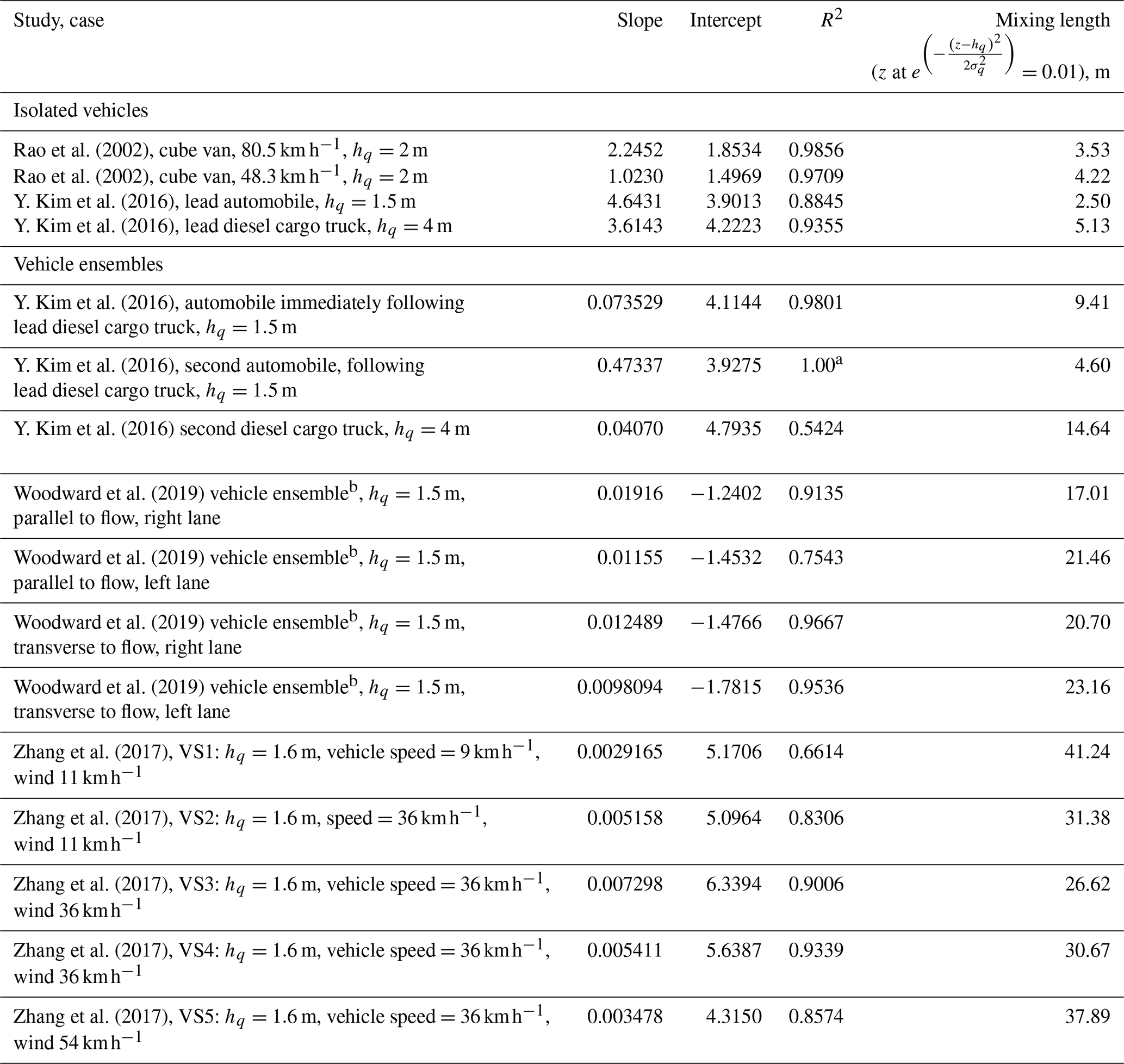
a Note that only two contour lines were available for retrieving TKE and height values from this vehicle within Fig. 14 of Y. Kim et al. (2016); while the correlation coefficient is formally unity, this is a two-point line.
b Woodward et al. (2019) Fig. 21 turbulent velocity components in the parallel and transverse directions were squared, and distances were scaled to give equivalent distances from wind-tunnel to ambient environment.

Figure 1Example of length scales associated with an ensemble of vehicles (after Y. Kim et al., 2016; Fig. 14). TKE contours along dashed lines were extracted and fit to Eqs. (1) and (2) for Table 1. Note that the length scale of turbulence immediately behind the leading vehicle, a large transport truck, is only 5.13 m, while the length scale immediately behind the trailing vehicle in the ensemble (an identical transport truck) is 14.73 m.
An example of the analysis used to construct Table 1 appears in Fig. 1 for a CFD example for an ensemble of vehicles, taken from the literature (Y. Kim et al., 2016). In this figure, contours of TKE are shown as solid lines. TKE values as a function of height at three locations behind the trucks were used to determine σq and hence estimate the length scale via Eqs. (1) and (2). A notable feature of this example is the substantial increase in length scale which occurs between the initial vehicle (a transport truck) and subsequent downwind vehicles (compare the height of TKE contours, and the resulting length scales in Fig. 1, between the left and right sides of the figure). Increases in downwind turbulent length scales associated with vehicles moving in close ensembles are a common feature in the literature.
This analysis (see Table 1) shows that a Gaussian distribution accounts for much of the variability in TKE with height (correlation coefficients of 0.54 to 0.99), and under realistic traffic conditions, the mixing lengths increase in size and may be considerably larger than those of isolated vehicles.
Two VIT mobile laboratory studies (Gordon et al., 2012; Miller et al., 2018) observed vehicle-per-second TKE for vehicles moving in ensembles along multilane roadways, aggregated by vehicle classes using the same methodology, to derive formulae for the net TKE added by VIT at 4 and 2 m (the height of the instrumentation used in these studies). We combine these data here to determine the change in VIT with height. Setting E as the TKE added due to the vehicles, two formulae result as follows:
where E(4 m) and E(2 m) are the TKE added driving within the ensemble at 4 and 2 m elevation from these two studies (m2 s−2) and Fc, Fm, and Ft are the number of passenger cars and mid-sized (vans, flatbed pickup trucks, and SUVs) and large vehicles (10 to 18 wheel heavy-duty vehicles) traveling past a given point on the highway per second. The numerical coefficients are the time-integrated TKE values (Iq) at the two heights (m2 s−1). An alternative approach would be to make use of vehicle speed data within each grid cell and parameterizations utilizing vehicle speed (Di Sabatino et al., 2003; Kastner-Klein et al., 2003) to construct TKE additions due to the sub-grid-scale roadways. However, vehicle speed information is not currently readily available on a gridded hourly basis, while estimates of vehicle kilometer traveled are available in gridded form due to their use in emissions processing, and making the simple scaling assumption that the vehicles travel across one dimension of a grid cell allows us to generate the Fc values required to estimate TKE. Note that vehicle speed is implicit in this methodology utilizing vehicle kilometer traveled (VKT) – higher speeds will result in a greater number of vehicle kilometers traveled per unit time and hence higher TKE values. As in the above discussion, we assume a Gaussian distribution of the coefficients of the TKE equations of Eq. (3) with height for each vehicle, where hq=1.5, 1.9, and 4.11 m for cars, mid-sized vehicles, and trucks, respectively, with each of the 2 and 4 m values of the coefficients of Eq. (3) being used to determine the corresponding values of Aq and σq of Eq. (1), (i.e., q= c, m, t). The resulting height-dependent formulae may be used to replace the coefficients of Eq. (3), leading to the following formula for the net turbulent kinetic energy associated with the number of vehicles in transit along a given stretch of roadway at a given time:
Most 3D chemical transport models make use of some variation in “K-theory” diffusion to link turbulent kinetic energy to mixing, with the vertical mixing of a transported variable c due to turbulence at heights z being related to the thermal turbulent transfer coefficient K via
Finite differences and tridiagonal matrix solvers are usually used to forward integrate Eq. (5). For example, the solver used in the Global Environmental Multiscale – Modelling Air-quality and CHemistry (GEM-MACH) model uses the following finite difference for the spatial derivatives (both spatial derivatives are O(Δσ2), the derivatives are carried out in, and the K values are transformed into, coordinates as , where P is the pressure and P0 is the surface pressure):
Note in Eq. (6) that the prognostic values of K calculated by the weather forecast model are on the same vertical levels as concentration; values of the additional component of K associated with VIT must therefore be calculated for model layers as opposed to layer interfaces.
K and E may be linked through the relationship of Prandtl, where l is a characteristic length scale:
As was done for Table 1, we have chosen this value on a per-vehicle basis as the vertical location at which the Gaussian profiles derived above reach 0.01 (i.e., 1 %) of their maximum value. Using each of the coefficient values of Eq. (3) at the two heights, in conjunction with Eq. (1) treated as a two variable in two unknowns (Aq, σq) problem we find values of lc, lm, and lt of 13.56, 6.25, and 11.28 m, respectively. These values are based on observed traffic conditions and fall well within the range of mixing lengths provided for vehicle ensembles in Table 1; however, we note that they are a source of uncertainty, with the percent uncertainties (Gordon et al., 2012) associated with the 4 m values at ±52 %, ±157 %, and ±12 % for cars, mid-sized vehicles, and trucks, respectively. The relatively low values of lm and high uncertainties in the corresponding mid-sized vehicle per-vehicle estimates of TKE relative to the other vehicle types are likely the result of a combination of small sample size (Gordon et al., 2012, noted the relative proportion of the three vehicle classes as 89.9 % cars, 4.8 % mid-sized vehicles, and 5.3 % trucks) and the variety of ensemble versus isolated vehicles sampled (noting the variation in Table 1 for vehicles within the smaller vehicle size classes). Additional observations of vehicle turbulence are clearly needed, particularly in the region above the largest vehicles on the road (4.1 m), using remote-sensing techniques such as Doppler lidar, in order to improve mixing length estimates. However, the values used here are reasonable with respect to the available data, and while they likely overestimate the mixing length associated with isolated vehicles (Rao et al., 2002; Y. Kim et al., 2016), they likely underestimate the mixing length of ensembles of vehicles (Y. Kim et al., 2016), particularly for ensembles moving within street canyons (Woodward et al., 2019; Zhang et al., 2017). The latter represent the some of the specific regions where vehicle emissions are likely to dominate.
We derive the following formula for the addition to the thermal turbulent transfer coefficient associated with vehicle passage as a function of height:
The use of Eq. (8) must be undertaken with care. Like most regional air-quality models, the vertical resolution of GEM-MACH used here is relatively coarse (the first four model layer midpoints are located approximately 24.9, 99.8, 205.0, and 327.0 m above the surface). Layer midpoint values must be representative of the layer resolution in order to describe the impact of VIT on the layer. A simple linear interpolation between the peak values of KVIT and the first model interface will overestimate the impact of VIT within the lowest model layer, while the use of Eq. (8) for the midpoint value alone will underestimate the influence of VIT within the lowest part of the first model layer. The best representation of a sub-grid-scale scalar quantity within a discrete model layer is its vertical average within that layer. Here, we calculate the vertically integrated average of Eq. (8) within each model layer, to provide the best estimate of the impact of VIT, to within the vertical resolution of the model.
2.3 VIT and model vertical resolution
The issue of the vertical extent of the impact of VIT is worth considering in the context of model layer thickness. Given that the vertical length scale of added VIT is on the order of tens of meters, as denoted in the studies quoted herein, it is reasonable to question whether the added turbulence should be expected to have an impact on the dispersion of pollutants. This apparent contradiction is easily resolved by noting (1) that the turbulence due to VIT is added as an addition to the pre-existing “meteorological” thermal turbulent transfer coefficient (with the net turbulence profile, not the VIT alone, determining its impact on vertical mixing) and (2) that the impact of this net turbulence does not depend just on the magnitude of the net coefficients of thermal turbulent transfer, but also on their vertical gradient. This second point can be illustrated by expanding the diffusion equation using the chain run of calculus (i.e., ) and the aid of an example, shown in Fig. 2. Figure 2 displays examples of cases where the concentration gradient and natural thermal turbulent transfer coefficient both decrease linearly with height (Fig. 2a and b) and where the concentration gradient decreases with height while the natural thermal turbulent transfer coefficients increase with height (Fig. 2c and d). The added KVIT is shown as a blue dashed line, and the net vertical thermal turbulent transfer is shown as a red line. Figure 2a and c depict these curves at a high vertical resolution, while Fig. 2b and d depict them at a low (regional model) resolution. Note that in the latter, the vehicle-induced addition to the net thermal turbulent transfer coefficient depicted in Fig. 2a and c lies entirely within the lowest model layer of Fig. 2b and d. In both Fig. 2a and b, the impact of KVIT is to slow the build-up of near-surface concentrations. In both Fig. 2c and d, the impact of KVIT is to more rapidly vent near-surface concentrations further up into the atmosphere. That is, at both high and low resolution, KVIT affects near-surface concentrations, due to the vertical gradient of . Centered difference calculations for the low-resolution case are shown in Fig. 2b and d to illustrate the point that gradients in low vertical-resolution net diffusivity result in reductions in the lowest model layer trapping and increases in venting from this lowest layer. In both of these cases, the addition of vehicle turbulence to the lowest model layer changes the gradient of the net thermal turbulent transfer coefficient, in turn leading to reduced surface concentrations. The above example illustrates the manner in which VIT may have an impact even on relatively low vertical model resolution.

Figure 2Illustration of the impact of VIT on the local vertical gradient of the thermal turbulent transfer coefficients, at high (a, c) and low (b, d) resolution. Purple, green, dashed blue, and red lines illustrate the height variation in concentration, meteorological, or natural coefficient of thermal turbulent transfer, VIT coefficient of thermal turbulent transfer, and net coefficient of thermal turbulent transfer, respectively. (a, b) High- and low-resolution profiles and gradients, for the case where both concentration and meteorological thermal turbulent transfer coefficients decrease with height. (c, d) High- and low-resolution profiles and gradients, for the case where concentration decreases and meteorological thermal turbulent transfer coefficients increases with height.
2.4 Relating VIT to available gridded data – vehicle kilometer traveled
Along individual roadways, Eq. (8) makes use of Fc, Fm, and Ft observations at points along roadways within a grid cell, hence deriving local estimates of VIT. These data are currently difficult to obtain for large-scale applications, and hence we have turned to secondary sources of information to estimate these three terms. VKT is used for estimating on-road vehicle emissions at jurisdiction level (e.g., county level for the US and province level for Canada) for national emissions inventories. Emissions processing systems used for air-quality models make use of spatial surrogates to help determine the spatial allocation of the mass emitted from different types of vehicles on different roadways (Adelman et al., 2017). The same set of surrogates is used for calculating VKT (km s−1) for each grid cell of the model domain (varying by hour of day and day of week, for each of the three vehicle categories listed (see Fig. 3), in turn providing diurnal variations in VIT matching traffic flow. The data shown are derived from 2006 Canadian (Brett Taylor, National Pollution Release Inventory, Environment and Climate Change Canada, personal communication, 2019) and 2011-based projected 2017 US VKT (EPA, 2017). Note that for the 10 km grid cell size used here, values of Fc, Fm, and Ft may be derived by dividing these numbers by 10. The largest contribution to total vehicle kilometer traveled is by the “cars” class (Fig. 3a) due to their greater numbers (the originating study (Miller et al., 2018) found that 89.9 % of vehicles measured were cars), followed by trucks (Fig. 3c; 5.3 % of vehicles measured) and mid-sized vehicles (Fig. 3b; 4.8 % of vehicles measured).
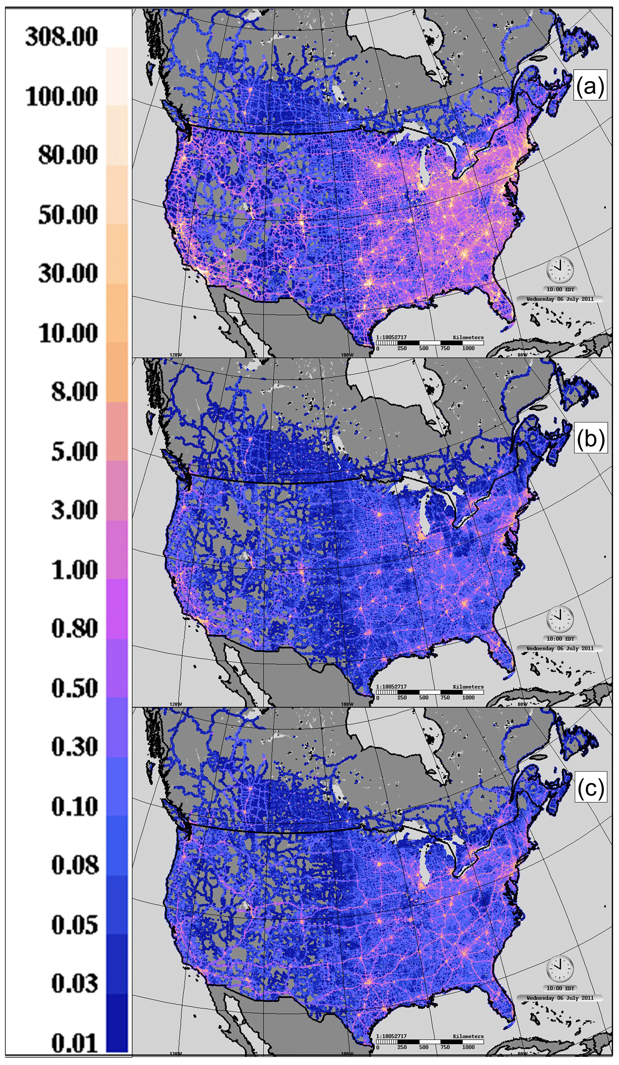
Figure 3Vehicle kilometer traveled per 10 km grid cell (km s−1) for (a) cars, (b) mid-size vehicles, and (c) trucks, July 2015.
These VKT data may be linked to the above VIT formula in Eq. (8), provided the distance each vehicle is traveling within that grid cell is known. Here, we have made two additional assumptions. The first assumption is that each vehicle carries out a simple transit of the cell – the distance traveled is the cell size. While this may be a reasonable first-order approximation, we note that it has limitations: for example, when the number of vehicles on the roads overwhelm the capacity of the roads (rush-hour traffic jams), the distance traveled decreases. However, under these circumstances the VKT values will also decrease; the impact of rush-hour conditions should to some extent be included within the VKT estimates available for emissions processing systems. The second assumption is that the VKT contributions within a grid cell are additive – i.e., that their numbers may be added via the “F” terms in Eq. (8) (Gordon et al., 2012; Miller et al., 2018), an assumption found to be accurate in CFD modeling (Y. Kim et al., 2016). Note that this assumption may result in overestimates of the net TKE – a better methodology for future work would be to collect and make use of statistics of vehicle density by roadway type within each grid cell. However, we note that assuming that vehicles are evenly distributed over roadways in a grid cell would result in a net underestimate of the TKE contributed over the larger roadways and main arteries of urban areas.
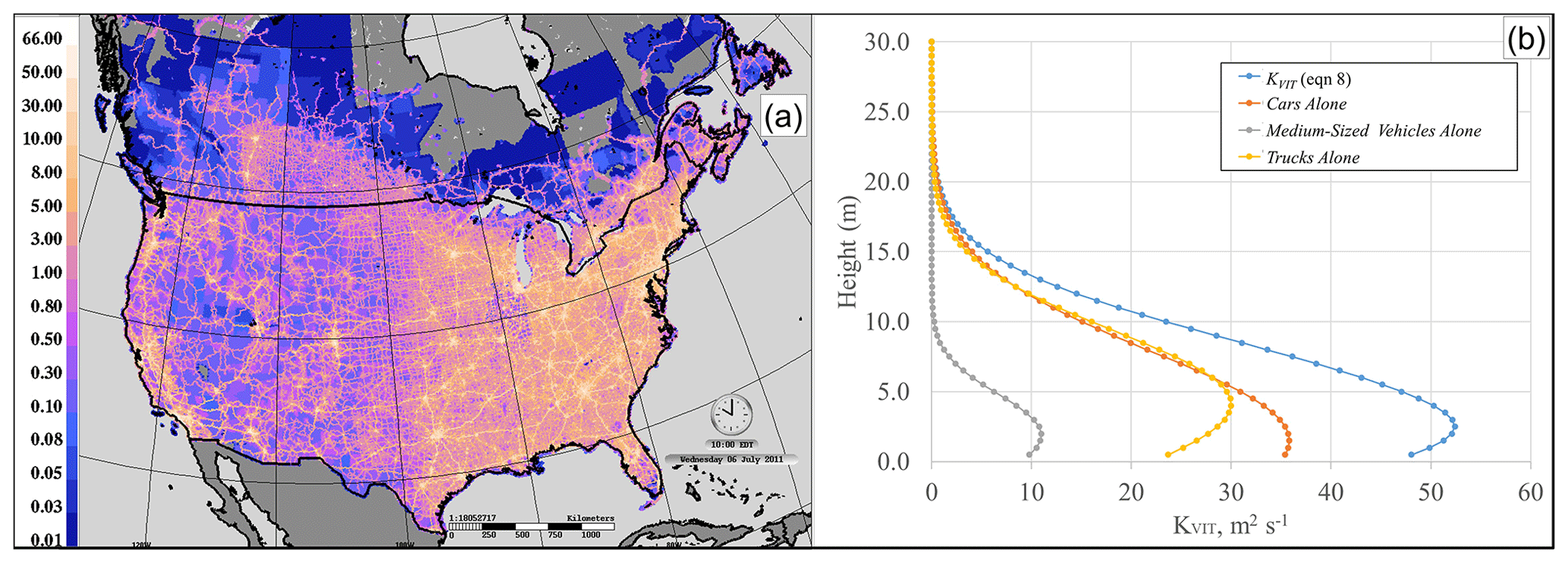
Figure 4(a) Example estimated thermal turbulent transfer coefficients from VIT at 2 m elevation during a weekday at 10:00 in July (m2 s−1), using the VKT data of Fig. 3. (b) Vertical profile of VIT thermal turbulent transfer coefficients at 1 m resolution in central Manhattan Island and individual values for the TKE associated with cars, mid-sized vehicles, and trucks considered separately, generated using Eq. (8). Note that the profiles of (b) would be added to the ambient thermal diffusivity coefficients (see Sect. 2.5 and Eq. 12).
An example of the gridded vehicle-induced thermal turbulent transfer coefficient values (KVIT, Eq. 8) created using these assumptions, at 10:00 EDT, for our North American 10 km resolution domain, is shown in Fig. 4a. An an example vertical profile of KVIT for central Manhattan Island at 0.5 m vertical resolution is shown in Fig. 4b. The resulting enhancements to “natural” K values at the vertical resolution of the version of the GEM-MACH air-quality model at 2.5 km horizontal resolution are shown in Fig. S1 in the Supplement as dashed lines. The enhancements are confined to the lowest model layer, as might be expected from the vertical resolution employed in this version of GEM-MACH. Nevertheless, the values are sufficient to significantly change simulated vertical transport due to modifications to the resolved gradient in thermal turbulent transfer coefficients, as discussed above. Both the magnitude and gradient of may contribute to the concentration changes: breaking the vertical diffusion equation down using the chain rule, Eq. (5) may be rewritten as
Both terms on the right-hand-side of Eq. (9) may contribute to decreases in concentration c at the surface and increases in concentrations aloft. If the near-surface concentration profile () is negative (concentrations decrease with height), then increases in K will result in surface concentration decreases). If this results in sufficient lofting that the concentration profile maximizes above the ground (i.e., becomes positive near the surface), then decreasing values of K with height (i.e., negative values of ) will also result in a shift towards negative rates of change, through the second term in the right-hand-side of Eq. (9). All six panels of Fig. S1 show increased Kvalues, i.e., increases in the first term in Eq. (9). All six panels also show a trend of becoming more negative (that is, near-surface positive slopes become less positive and negative slopes become more negative), decreasing the magnitude of the second term in Eq. (9) in Fig. S1b–d and f and switching to a negative rate of change in Fig. S1a and e. Both changes in the magnitude and gradient of K resulting from VIT contribute to the resulting changes in surface concentration.
The thermal turbulent transfer coefficient values of Fig. S1 may also be compared to the minima on natural K values imposed in air pollution models in an attempt to account for missing subgrid-scale mixing (Makar et al., 2014; these are typically on the order of 0.1 to 2.0 m2 s−1). Aside from Fig. S1a, the vertical profiles here would not be modified by these lower limits. We also note that these VIT-induced changes in total thermal turbulent transfer coefficients only impact the species emitted at the roadway level, as discussed below.
2.5 Construction of a sub-grid-scale parameterization for on-road vehicle-induced turbulence
We note that the portion of the area of a grid cell which is roadway-covered will be relatively small for most air pollution model resolutions, such as those considered here. For example, satellite imagery of the largest freeways show these to have a width of less than 400 m. Hence, the largest roads make up less than of the total area of a 2.5 km grid cell, and less than of a 10 km grid cell). The largest impact of VIT is thus likely to be for the chemical species being emitted by the mobile sources, in terms of the grid cell average concentration. Furthermore, the grid cell approach common to these models results in horizontal numerical diffusion from the roadway scale to the grid cell scale: sub-grid-cell-scale emissions are automatically mixed across the extent of the grid cell. The key impact of VIT will thus be in the vertical dispersion of the pollutants emitted from mobile sources. We must therefore devise a numerical means to ensure this additional source of diffusion is added to the model, bearing these constraints in mind.
Two examples of similar sub-grid-scale processes appear in the literature. The first example is the cloud convection parameterizations used in numerical weather forecast models (Kain, 2004), wherein the formation and vertical transport associated with convective clouds, known to occur at smaller scales than the grid cell size employed in a numerical weather prediction model, are treated using sub-grid-scale parameterizations. In these parameterizations, cloud formation and transport are calculated within the grid cell on a statistical basis, using formulae linking the local processes to the resolvable scale of the model. The second example is found in the treatment of emissions from large stacks within air-quality forecast models (Gordon et al., 2018; Akingunola et al., 2018). These sources usually have stack diameters on the order less than 10 m, and these sources emit large amounts of pollutant mass at high temperatures and velocities. In order to represent these sources, the most common approach is to calculate the height of the buoyant plume using the predicted ambient meteorology (vertical temperature profile, etc.) as well as the stack parameters (exit velocity, exit temperature, stack diameter). The emitted mass during the model time step from the stack is then distributed over a defined vertical region within the grid cell in which the source resides. Note that the mass is also automatically distributed immediately in the horizontal dimension within the grid cell – the key issue is to ensure that the emitted mass is properly distributed in the vertical dimension. Our aim in the VIT parameterization that follows is identical in intent to that of the existing major point source treatments in air-quality models: to redistribute the mass emitted by vehicle sources in the vertical dimension, taking the very local physics influencing that vertical transport of fresh emissions into account. We therefore focus on determining the at-source vertical transport of emitted mass associated with VIT.
We start with the formulae for the transport of chemical species by vertical diffusion:
where ci is the emitted chemical species, K represents the sum of all forms of thermal turbulent transfer in the grid cell, and Ei is the emissions source term for the species emitted at the surface (applied as a lower boundary condition on the diffusion equation). For grid cells containing roadways and hence mobile emissions, we split K into meteorological and vehicle-induced components (KT and KVIT, respectively) and the emissions into those from mobile sources and those from all other sources (Ei,mob and Ei,oth, respectively):
The terms in Eq. (11) may be rearranged:
The first bracketed term in Eq. (12) describes the rate of change of the chemical's concentration due to its emission by non-mobile area sources and vertical diffusion due to meteorological sources of turbulence within the grid cell but outside of the sub-grid-scale roadway. The second term describes the rate of change in the vertical diffusion of the mobile-source-emitted pollutants over the sub-grid cell roadway, which experiences both meteorological and roadway turbulence, and the final term prevents double-counting of the meteorological component in Eq. (11), which is equivalent to Eq. (12). Note that turbulent mixing for non-emitted chemicals is determined by solving Eq. (5), and for chemicals which are not emitted from mobile on-road sources, Eq. (10) is solved with . This form of the diffusion Eq. (12) allows the net change in concentration to be calculated from three successive calls of the diffusion solver, starting from the same initial concentration field. One advantage of this approach is that existing code modules for the solution of the vertical diffusion equation may be used – rather than being used once, they are used three times, with different values for the input coefficients of thermal turbulent transfer coefficient (K) and for the lower boundary conditions (E). The solution, once a suitable means of estimating KVIT is available, is thus relatively easy to implement in existing numerical air pollution model frameworks.
2.6 Comparison of energy densities: VIT, solar, and urban perturbations in sensible and latent heat
The relative contribution of TKE from VIT towards energy density can be compared to the daytime solar maximum energy input to illustrate why VKT has relatively little impact during daylight hours, particularly in the summer. The maximum TKE from VIT can be determined easily from Fig. 3 and the use of our formulae; Fig. 3a shows vehicle kilometer traveled values ranging from a maximum of 308 in the highest density 10 km grid cell in North America (New York City) down through 4 orders of magnitude in background grid cells with few vehicles. A typical urban value would be 30.8 VKT: this gives an Fc value from our formulae of 3.08 vehicles s−1 for a 10 km grid cell size. Assuming that the vehicles are all cars, from our formulae we have a corresponding total TKE added at the point crossed by the vehicles, at height m, of 7.48 m2 s−2. We can combine this and the Fc value along with the area and volume of a lane of a roadway to estimate the energy density (EVIT) on dimensional grounds:
Assuming each vehicle has a length of 4.5 m, width of 2.0 m, height of 1.5 m, a lane length of 10 km, and an air density of 1.225 kg m−3, one arrives at 84.8 kg s−3 and values ranging from a North American grid maximum of 848 kg s−3 to a background value 4 orders of magnitude smaller ( kg s−3). These energy densities may be compared to the typical solar energy density reaching the surface at midlatitudes of 1300 W m−2, or in SI units, 1300 kg s−3, and the typical range of perturbations in latent and sensible heat fluxes associated with the use of a more complex urban radiative transfer scheme (the town energy balance module; Mason, 2000) in our 2.5 km grid cell size simulations (typical diurnal ranges in the perturbations associated with versus without the use of the town energy balance (TEB): latent, −200 to +3 W m−2; sensible, −100 to +100 W m−2, respectively). That is, under most daylight conditions, the energy densities associated with VIT will be relatively small compared to the solar energy density at midday, with a typical urban value of 6.5 % and a range from 65 % in the cell with the highest VKT values down to 0.0065 % in background conditions where the vehicle numbers are relatively small. Urban traffic however may contribute similar energy levels as the changes in net latent and sensible heat fluxes associated with the use of an urban canopy radiative transfer model. We also note that at night, during the low sun angle conditions of early dawn and late evening and during the lower sun angles of winter, the relative importance of VIT to solar radiative input will be larger. Consequently, the impact of VIT will be higher at night and in the early morning rush hours and at other times when the sun is down or sun angles are low, as is demonstrated below.
2.7 GEM-MACH simulations
A research version of the Global Environmental Multiscale – Modelling Air-quality and CHemistry (GEM-MACH) numerical air-quality model, based on version 2.0.3 of the GEM-MACH platform, was used for the simulations carried out here (Makar et al., 2017; Moran et al., 2010, 2018; Chen et al., 2020). GEM-MACH is a comprehensive 3D deterministic predictive numerical transport model, with process modules for gas and aqueous phase chemistry, inorganic particle thermodynamics, secondary organic aerosol formation, vertical diffusion (in which area sources such as vehicle emissions are treated as lower boundary conditions on the vertical diffusion equation), advective transport, and particle microphysics and deposition. The model makes use of a sectional approach for the aerosol size distribution, here employing 12 aerosol bins. The version used here also follows the “fully coupled” paradigm – the aerosols formed in the model's chemical modules in turn may modify the model's meteorology via the direct and indirect effects (Makar et al., 2015a, b, 2017). The meteorological model forming the basis of the simulations carried out here is version 4.9.8 of the Global Environmental Multiscale weather forecast model (Cote et al., 1998a, b; Caron et al., 2015; Milbrandt et al., 2016). Emissions for the simulations conducted here were created from the most recent available inventories at the time the simulations were carried out – the 2015 Canadian area and point source emissions inventory, 2013 Canadian transportation (on-road and off-road) emissions inventory, and 2011-based projected 2017 US emissions inventory. As noted above, the model simulations were carried out on two separate model domains shown in Fig. 5: a 10 km horizontal grid cell size North American domain (768×638 grid cells; 7680×6380 km) and a 2.5 km horizontal grid cell size Pan Am Games domain (520×420 grid cells; 1300 km×1050 km). For the 10 km domain, simulations were for the month of July 2016, while for the higher-resolution model, month-long summer (July 2015) and winter (January 2016) simulations were carried out with and without the VIT parameterization. These periods were based on the availability of emissions data, previous model simulations for the same time periods appearing in the literature (Makar et al., 2017; Stroud et al., 2020), and the timing of a prior field study (Stroud et al., 2020).

Figure 5GEM-MACH test domains: (a) 10 km grid cell size North American domain; (b) 2.5 km grid cell size Pan Am domain.
2.8 VIT as a sub-grid-scale phenomena
It should be noted that the VIT enhancements to turbulent exchange coefficients are used to determine the vertical distribution of freshly emitted pollutants at each model time step – they are not applied for all species within a model grid cell. Similar sub-grid-scale approaches are used for the vertical redistribution of mass from large stack sources of pollutants, where buoyancy calculations are applied to determine the rise and vertical distribution of pollutants from large industrial sources. Both stacks and roadways are treated as sub-grid-scale sources of pollutants which are influenced by very local sources of energy (stacks: high emission temperatures and exit velocities; roadways: vehicle-induced turbulence) resulting in an enhanced vertical redistribution of newly emitted chemical species. In both cases, the vertical transport results from an interplay between the energy associated with the emission process (stacks: high temperature emissions with the ambient vertical temperature profile; VIT: kinetic energy imparted to the atmosphere in which emissions have been injected with the ambient turbulent kinetic energy). This interaction precludes a treatment solely from the standpoint of model input emissions, since the extent of the mixing will depend on the local atmospheric conditions as well as the energy added due to the manner in which the emissions occur. Both processes have been addressed by large eddy simulation modeling on a very local scale, but parameterizations are required in both cases for regional-scale simulations. In both cases, the parameterized vertical redistribution of pollutants is applied to freshly emitted species – the horizontal spatial extent of the emitting region is sufficiently small that although present, the enhanced mixing will have a minor effect on the redistribution of pre-existing chemicals and on other atmospheric constituents affected by vertical transport. VIT in the context of regional chemical transport models is thus best treated as a sub-grid-scale phenomenon applied to fresh emissions, in direct analogy to the approach taken for large stack emissions.
3.1 VIT height dependence as a Gaussian distribution
In the Methodology section, we describe the potential for the use of a Gaussian distribution to describe the fall-off in TKE with height above vehicles. Using the equations presented there, we have analyzed VIT studies appearing in the literature, determining the decrease in TKE as a function of height from published figures and then fitting these data to a Gaussian distribution to the height above ground. The result of this analysis for several data sets is shown in Table 1, generated by extracting vehicle centerline TKE values from contour plots of published data, and is subdivided into isolated vehicle and vehicle ensemble studies and cases.
The inferred mixing length shows a marked variation between that of isolated vehicles or the lead vehicle in an ensemble and that of other vehicles appearing further back in the ensemble. Both directly observed and CFD modeled values of the inferred mixing length for isolated vehicles or the lead vehicles of an ensemble vary from 2.5 to 5.13 m. For subsequent vehicles in an ensemble, the mixing lengths increase to range from 4.6 to 41 m. The difference in mixing length between the lead vehicle in an ensemble and subsequent identical vehicles appearing later in the ensemble also increases. For example note that diesel truck mixing lengths inferred from the CFD modeling examining different vehicle configurations (Y. Kim et al., 2016) increase from 5.13 to 14.64 m, and the mixing lengths for automobiles increase from 2.50 (isolated automobile) to 4.6 (automobile two vehicles back from a lead diesel truck) to 9.41 m (automobile immediately behind a leading diesel truck). The mixing length associated with VIT may also be significantly influenced by the ambient wind and local built environment – the mixing length associated with the component of TKE due to VIT within street canyons (Woodward et al., 2019; Zhang et al., 2017) ranges from to greater than the street canyon height, with maximum mixing lengths of 41 m. It is important to note that these mixing lengths are driven by the vehicle passage within the canyon; they result from the additional TKE added due to the presence of vehicles in the CFD simulations. The above data show that a Gaussian distribution provides a reasonable description of the decrease in TKE from vehicles with height, and, under realistic traffic conditions, the mixing lengths increase in size and are considerably larger than those of isolated vehicles and are comparable to or greater than the near-surface vertical discretization of air-quality models.
The length scales associated with VIT range from 2.50 m in the case of isolated vehicles (Y. Kim et al., 2016), through ∼10 m for vehicles moving in ensembles (Woodward et al., 2019; Zhang et al., 2017) up to 41 m, with the larger values being typical for urban street canyons. The latter describe the specific regions in which VIT is expected to have the greatest impact, given the high vehicle density within the urban core. However, our parameterization makes use of length scales derived from observations on open (non-street canyon) freeways (Gordon et al. 2012; Miller et al., 2018) and thus may underestimate the length scales in the urban core. The impact of multiple vehicles traveling in an ensemble on open roadways was specifically depicted in the open roadway simulations of Y. Kim et al. (2016) reproduced in Fig. 1, where the vertical extent of turbulent mixing was shown to grow with increasing number of vehicles traveling in an ensemble. Furthermore, as was discussed and demonstrated in the Methodology section using the diffusivity equation, the length scale of the turbulence need not be greater than the model lowest layer resolution in order to capture the impacts of VIT on mixing, being due in part to the gradient in turbulence with height.
3.2 Model domains and evaluation data
Our 3D air-quality model (GEM-MACH) and our VIT parameterization, including its diurnal variation, are described in the Methodology section. Two air-quality model grid cell size and domain configurations were used for our simulations. The first employs a 10 km grid cell size with a North American domain and is used for the current operational GEM-MACH air-quality forecast (Moran et al., 2010, 2018; Fig. 5a). The second was a 2.5 km grid cell resolution domain focused on the region between southern Ontario, Quebec, and the northeastern USA (Joe et al., 2018; Ren et al., 2020; Stroud et al., 2020; Fig. 5b).
The impact of VIT was determined through paired model simulations, with and without the VIT parameterization, evaluated against the surface monitoring network data. The latter include hourly model output for ozone (O3), nitrogen dioxide (NO2), and particulate matter with diameters less than 2.5 µm (PM2.5), across North America and in our high-resolution eastern North America domain, evaluated at observation station locations with data from the Air Quality System (AQS, US EPA, 2021) and National Air Pollution Surveillance (NAPS, Government of Canada, 2021) networks. Observation station locations used in simulation evaluation for these species are shown in Fig. 6 for the two model configurations. The juxtaposition of observation stations with urban populations (where the highest vehicle density may be found) may be seen by comparing Fig. 6 with Fig. S2.
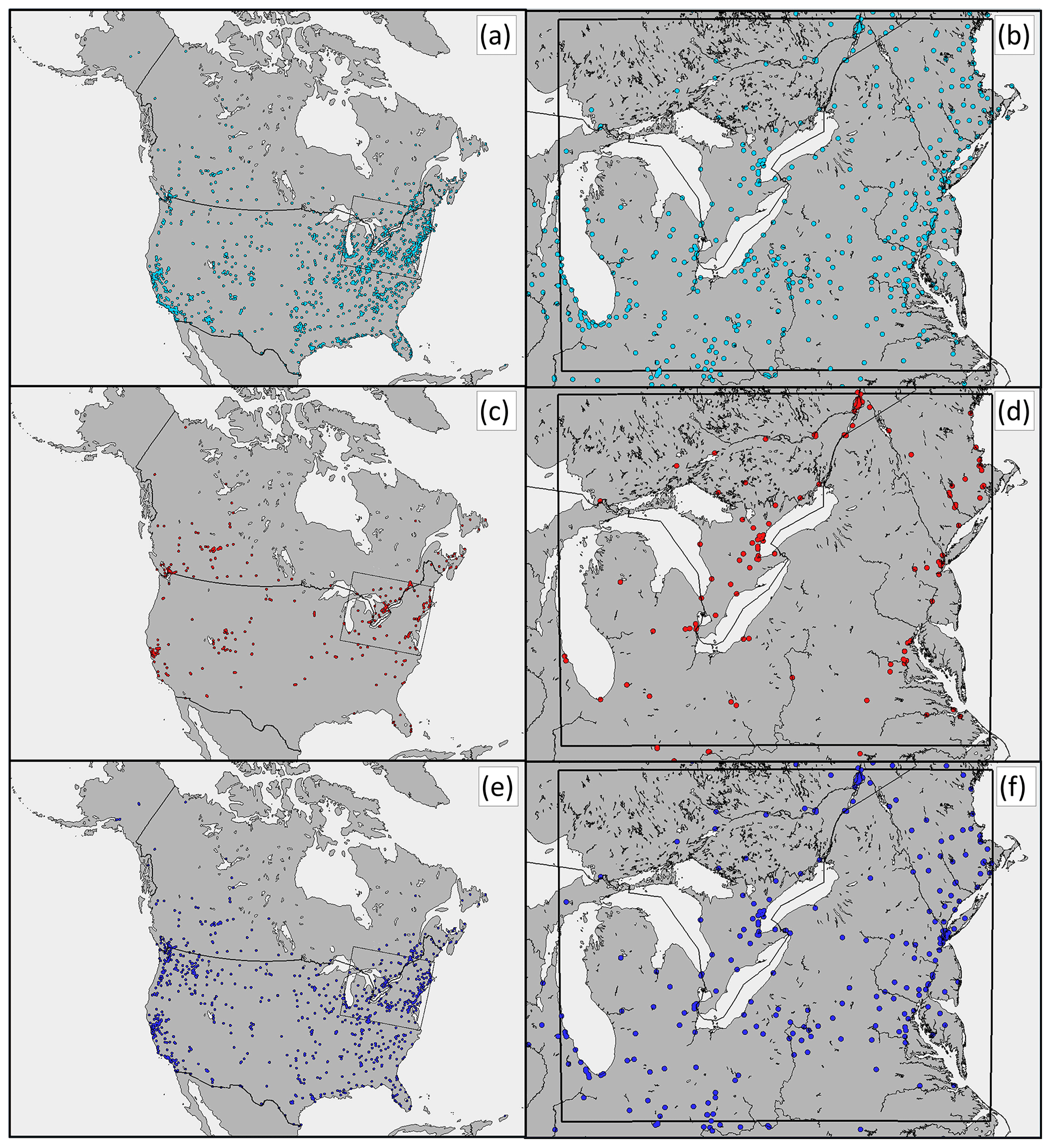
Figure 6AQS and NAPS hourly observation station locations for ozone (a, b), nitrogen dioxide (c, d), and particulate matter with diameters less than 2.5 µm (e, f). (a, c, e) Stations used for the 10 km grid cell size domain evaluation. (b, d, f) Stations used for the 2.5 km grid cell size domain evaluation (all stations located within central box).
3.3 Continental 10 km grid cell size domain evaluation
Simulations were carried out for the month of July 2016 for the 10 km grid cell size North American domain. Model performance metrics used to here are described in Table S1 in the Supplement and provided for the 10 km resolution “VIT” and “No VIT” simulations relative to the hourly observation data for PM2.5, NO2, and O3 in Table 2. These three chemicals were chosen due to their well-known link to human-health impacts of air pollution (Steib et al., 2008; Abelsohn and Steib, 2011).
Table 2Model performance for NO2, PM2.5, and O3 in the 10 km grid cell size North American domain. No VIT refers to simulations without vehicle-induced turbulence, and VIT refers to the simulation incorporating vehicle-induced turbulence. Bold-face print identifies the better score, italics the worse score, and regular font indicates similar performance between the two simulations for each metric and chemical species compared.
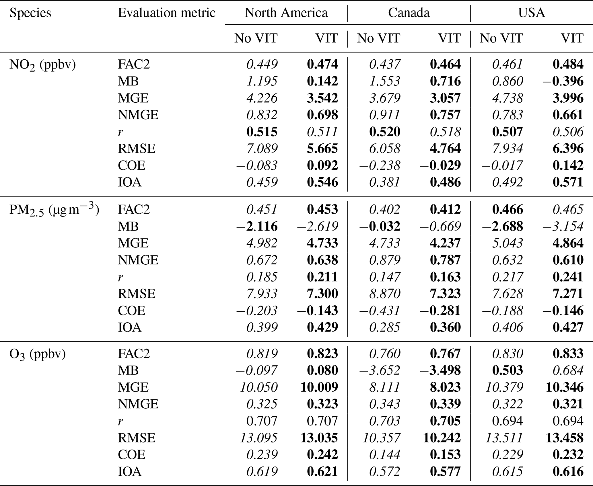
FAC2: number of model values within a factor of 2 of observations; MB: mean bias; MGE: mean gross error; NMGE: normalized mean gross error; r: Pearson correlation coefficient; RMSE: root mean square error; COE: coefficient of error; IOA: index of agreement. Formulae defining all terms appear in Table S1.
The addition of VIT improved the scores for most performance metrics (bold-face print in Table 2). For NO2, the addition of VIT improved all scores with the exception of the correlation coefficient, which was degraded in the third digit. All PM2.5 scores improved, with the exception of the mean bias, which became more negative by 0.5 µg m−3 across North America. All ozone scores improved, the exceptions being the correlation coefficient (which was the same for both simulations or improved in the third digit depending on the domain or country) and the ozone mean bias for the USA (which increased by +0.18 ppbv). Some of the improvements were substantial, when considered in a relative sense: this was most noticeable for the NO2 scores, with the North American mean bias for NO2 improving by a factor of 8.4, the mean gross error and index of agreement by 19 %, the root mean square error by 25 %, and the FAC2 score by 6 %. Relative improvements for PM2.5 across North America were more modest (ranging from 0.3 % for FAC2 to 14 % for the correlation coefficient). The corresponding relative changes for O3 ranged from a 22 % reduction in the mean bias magnitude to a fraction of a percent improvement for FAC2, mean gross error, root mean square error, and index of agreement. Overall, the model performance for the continental 10 km domain July 2016 simulations improved across different metrics, indicating that the increased vertical turbulent mixing resulting from the incorporation of VIT results in a more accurate representation of atmospheric mixing and chemistry.
Following the above comparison using all available surface monitoring network data (Table 2), we carried out a further evaluation where the stations were selected based on human population within grid cells (Fig. S2a), with only those stations in which the population exceeded 800 km−2 used for analysis. The results of this evaluation are shown in Table S2, which may be compared to Table 2 to show the relative influence of VIT on high-population areas. We note that the magnitude of the improvement in model performance associated with VIT has increased for many statistics when high-population (i.e., high vehicle traffic) areas are examined separately in this manner; for example the incremental improvement in North American NO2 mean bias changes from 1.053 ppbv for all stations versus 1.782 for population >800 km−2 stations, and the incremental improvement in PM2.5 MGE for North America changes from 0.249 to 0.665 µg m−3 (both numbers are differences between No VIT and VIT values in Tables 2 and S2 in each case). The number of model performance improvements with the use of VIT has increased when grid cells with populations greater than 800 km−2 are evaluated (62 out of 72 metrics improved with the use of VIT in Table 2, while 66 out of 72 metrics improved for stations corresponding to grid cells with populations greater than 800 km−2). Most of these additional improvements were associated with better ozone prediction performance in urban regions.
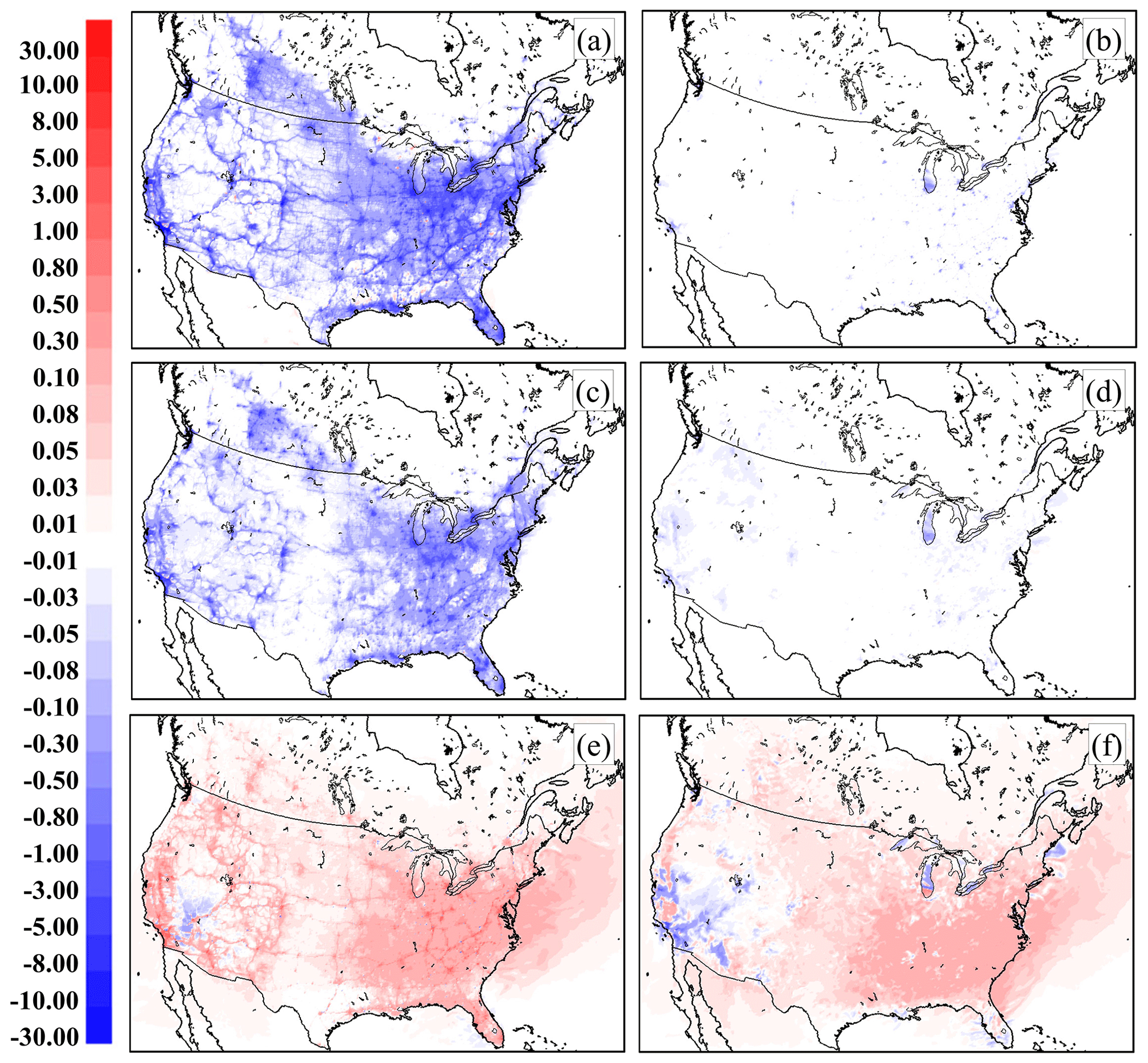
Figure 7Difference in 29 d average NO2, PM2.5, and O3, July 2016 continental 10 km domain simulations (VIT simulation–No VIT simulation). Averages are paired at (a, c, e) 10:00 UTC and (b, d, f) 22:00 UTC according to species: (a, b) ΔNO2 (ppbv); (c, d) ΔPM2.5 (µg m−3); (e, f) ΔO3 (ppbv).
The timing and spatial distribution of the differences in the 29 d mean values of NO2, PM2.5, and O3 at 10:00 and 22:00 UTC (06:00 and 18:00 EDT) are shown in Fig. 7. NO2 and PM2.5 have decreased in the urban areas and along the major road networks in the early morning (Fig. 7a and c), while the ozone (Fig. 7e) increases in the urban areas and along the roadways, with a minor increase in the surrounding countryside. The VIT effect occurs at night and in the early morning: the average differences are minimal by 18:00 EDT (Fig. 7b, d, and f). This diurnal cycle of the average impact of VIT is expected: at night and during the early morning the radiative-transfer-driven atmosphere is relatively stable, natural background turbulence is low in magnitude, and the relative contribution of VIT is therefore large. The reverse is true during the later morning to late afternoon, as the solar radiative balance causes near-surface turbulence to rise several orders of magnitude relative to nighttime values, and the relative contribution of VIT at those times becomes minimal. The strongest contribution of VIT thus occurs under more stable atmospheric conditions: at night and in the early morning.
The significance of the differences between VIT and no-VIT simulations was estimated using 90 % confidence levels, expressed here as confidence ratios. The difference between the mean values of the two simulations (MVIT, MNoVIT) becomes significant at a confidence level c if the regions defined by and do not overlap (where N is the number of grid point values averaged, the σ values are the standard deviations of the means, and z* is the value of the percentile point for the fractional confidence interval c of the normal distribution, where at c=0.90). Grid cell values where the mean values differ at or above the 90 % confidence level are thus defined as the confidence ratio:
where, when and the other terms are as described above, a CR value greater than unity defines the difference between the model simulations at that grid point as being significantly different at greater than the 90 % confidence level. The mean values at each grid point and their standard deviations may thus be used to determine the confidence ratio at each grid point – these values for each of the mean differences of Fig. 7 are shown in Fig. 8, where the color scaling in Fig. 8 and other confidence ratio figures which follow use red colors to indicate differences which are significant at greater than 90 % confidence. Grid point differences which exceed the 90 % confidence level requirement to progressively higher degrees are shown as progressively darker red colors, while differences falling progressively further below the 90 % confidence level requirement are shown as progressively lighter blue colors in these figures.

Figure 8The 90 % confidence ratio values (see Eq. 14) for the 29 d NO2, PM2.5, and O3 July 2016 continental 10 km domain simulations. Panels arranged as in Fig. 7: (a, c, e) 10:00 UTC, (b, d, f) 22:00 UTC; (a, b) NO2, (c, d) PM2.5, (e, f) O3. Values>1.0 indicate that the simulations differ at greater than 90 % confidence.
From Fig. 8, it can be seen that the continental-scale model means for the VIT versus No VIT simulations for surface NO2, surface PM2.5, and surface O3 at night differ at 90 % confidence over much of the domain for NO2 and PM2.5, and in urban core areas for O3. The spatial extent of 90 % confidence is much greater under the stable conditions of night (Fig. 8a, c, and e) than the less stable conditions of daytime (Fig. 8b, d, and f), as would be expected from the relative magnitude of KT versus KVIT during the day and night. While the nighttime influence of VIT on NO2 extends over much of the continent, for O3, the impact is primarily within the cities, where the increased mixing of NOx results in higher nighttime O3 concentrations due to decreased NOx titration.
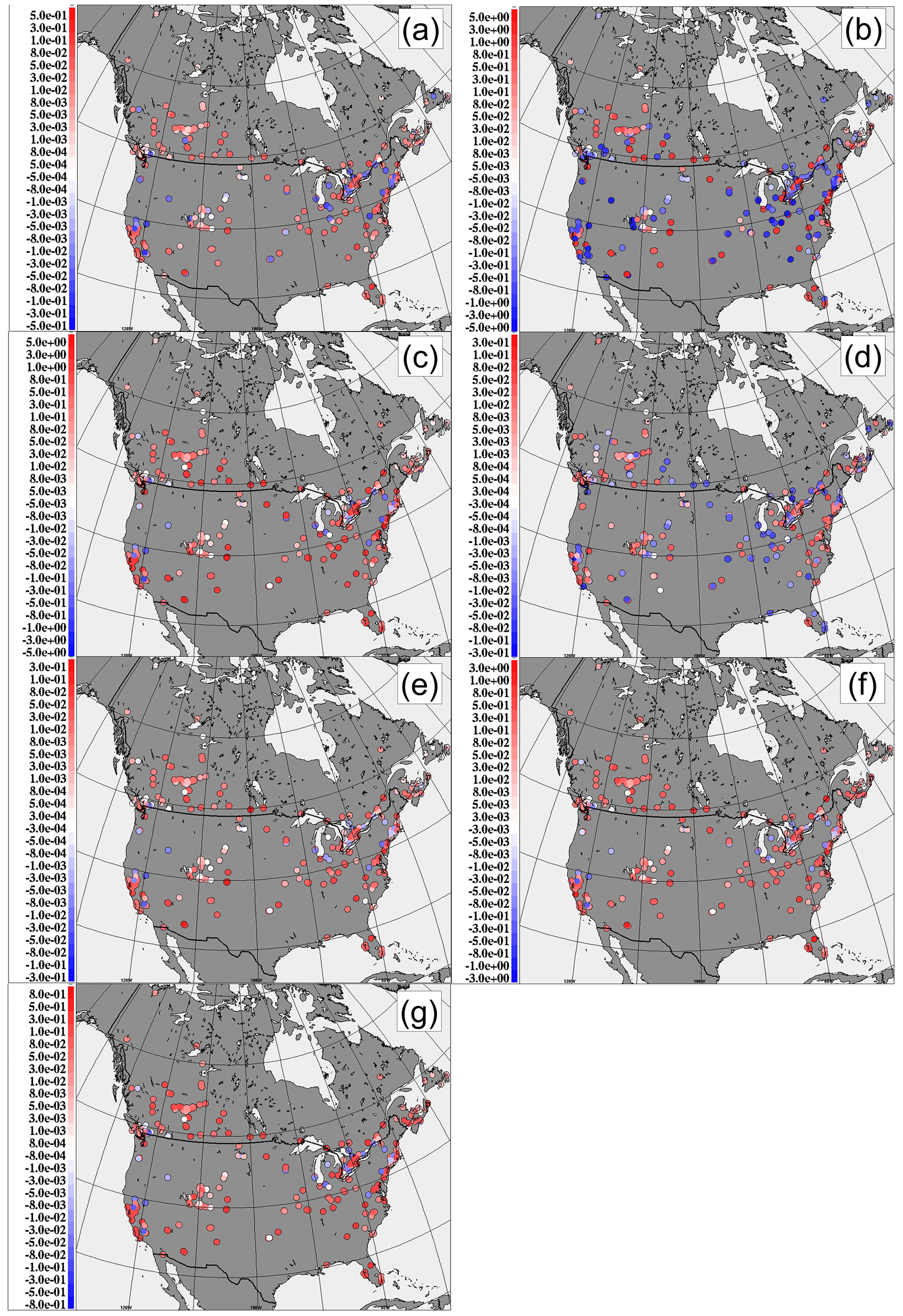
Figure 9Change in model NO2 performance at 358 North American surface monitoring sites, July 2016 (ppbv). Red colors indicate stations where the addition of the VIT parameterization improved model performance; blue colors indicate stations where the addition of the VIT parameterization degraded model performance. (a) ΔFAC2VIT–No VIT; (b) Δ|MB|No VIT–VIT; (c) ΔMGENo VIT–VIT; (d) ΔrVIT–No VIT; (e) ΔRMSENo VIT–VIT; (f) ΔCOEVIT–No VIT; (g) ΔIOAVIT–No VIT.
The all-domain model performance metrics of Table 2 were also calculated for each measurement station, and the appropriate differences in the metrics or their absolute values were used to determine location-specific impacts of the VIT parameterization for NO2, PM2.5, and O3 (Figs. 9, S3, and S4). Differences in the values of the metrics between the two simulations are shown, with the sign of the differences arranged so that red (blue) colors indicate better performance for the VIT (No VIT) simulations, respectively, red indicating better scores for the VIT simulation. The color scales in these figures are arranged to include 3 orders of magnitude between the lowest and highest difference scores and zero and to encompass the maximum value of the differences observed across all stations. The values vary between metrics and the chemical species, with the largest changes occurring for NO2, followed by PM2.5, and the smallest changes for O3, relative to typical concentrations of these species, and in accordance with Table 2. NO2 performance improvements with the VIT simulation (red colors) occur across most stations for the FAC2, MGE, RMSE, COE, and IOA scores (Fig. 9a, c, e, f, and g), while r and scores are more variable, with some stations having better performance for the No VIT simulation. PM2.5 performance improvements are more mixed, with large improvements for correlation coefficient (Fig. S3d) and IOA (Fig. S3g, a mild but overall positive effect of VIT for MGE, RMSE, and COE (Fig. S3c, e, and f), and more stations showing a degradation of performance for FAC2 and , echoing the net effect for these last two metrics seen in Table 2. O3 performance shows a strong regional variation (Fig. S4): most scores improve with the use of the VIT parameterization in the western and northeastern parts of the continent and degrade in the southeastern USA. The degradation in the southeast (e.g., increases in O3 concentrations in a region which already experiences a positive O3 bias) are associated with the transport of urban O3 precursors into forested areas in the region, with additional O3 production occurring there. These effects may be removed through the introduction of an additional parameterization for the reduced turbulence and shading within forested canopies (Makar et al., 2017; Fig. S5), with the combined parameterizations resulting in improvements in both NO2 and O3 performance. While the use of VIT degrades O3 performance in this region, this degradation is thus very small relative to the large improvements noted with the canopy effect (see Makar et al., 2017; Fig. S5 and its associated discussion). Another significant feature is the improvement (red colors) in most O3 station scores in urban regions (Fig. S4). These improved scores largely result from increases in ozone in the early morning hours (Fig. 7e), where VIT has resulted in increased vertical mixing and reducing surface level NOx and hence NOx titration of ozone, and also from mixing higher ozone levels aloft down into the lowest model layer.
Overall, the impact of the VIT parameterization was to improve North American simulation accuracy, across multiple statistical metrics, with the most significant improvements in the model performance for simulated NO2. Spatially, model performance was generally greatest in urban regions and western and northeastern North America, although this depends on the chemical species and the performance metric chosen.
3.4 Eastern North America 2.5 km grid cell size domain evaluation
With the use of a smaller grid cell size (i.e., “higher resolution”), meteorological models and on-line air-quality models such as GEM-MACH have the option of employing theoretical approaches which better simulate the more complex radiative transfer and physical environment-induced turbulence of urban areas. Urban heat islands are known to have a significant effect on turbulence, for example (Mason, 2000; Makar et al., 2006). In these simulations, we make use of the TEB (Mason, 2000; Leroyer et al., 2014; Lemonsu et al., 2010), a single-layer urban canopy module which solves the equations for urban atmosphere's surface and energy budgets for a variety of urban elements (roads, walls, roofs) and then aggregates the results for the net urban canopy. Such parameterizations are inappropriate for use in larger grid cell size models due to the latter's inability to resolve individual surface types and spatial gradients at the city scale. An important consideration in determining the relative importance of vehicle-induced turbulence is whether improvements in performance still occur, when these other sources of turbulent kinetic energy are included explicitly. We address this issue in our 2.5 km grid cell size modeling by employing the TEB parameterization for both VIT and No VIT simulations and evaluating both simulations against surface monitoring network observations as before. Both summer and winter simulations were carried out on the blue domain of Fig. 5b, and the same performance metrics were calculated as for the larger North American simulations (Table 3).
Table 3Model performance for NO2, PM2.5, and O3 in the 2.5 km grid cell size Pan Am domain. No VIT refers to simulations without vehicle-induced turbulence, and VIT refers to the simulation incorporating vehicle-induced turbulence. Bold-face print identifies the better score, italics the worse score, and regular font indicates similar performance between the two simulations for each metric and chemical species compared.

A similar pattern of performance improvement can be seen between 10 and 2.5 km grid cell size domains, comparing Tables 2 and 3, with improvements due to the use of VIT predominating in both summer and winter: despite the addition of a more explicit urban radiative balance approach, better scores were achieved with the addition of the VIT parameterization. Note that comparisons between the 2.5 and 10 km simulations for similar emissions inputs appear elsewhere in the literature (Stroud et al., 2020). The number of improved scores increases from summer to winter. Stable atmospheric conditions and low meteorological turbulence levels are more common in winter than summer, during both day and night, and the impact of the additional source of turbulence is thus proportionally stronger in the winter season. The VIT effects at the urban scale are the strongest for NO2 and PM2.5 and less noticeable for simulated O3, similar to the North American domain simulation. The largest improvements for the three species and across seasons occur for winter PM2.5, with the improved performance taking place in the first or second digit of the given metric. Metric differences for NO2 aside from mean bias occur in the second to third digit in the winter, with summer differences occurring in the first to second digit. Changes to O3 are relatively minor, with some improvements and degradation in performance in the third digits across the different metrics.
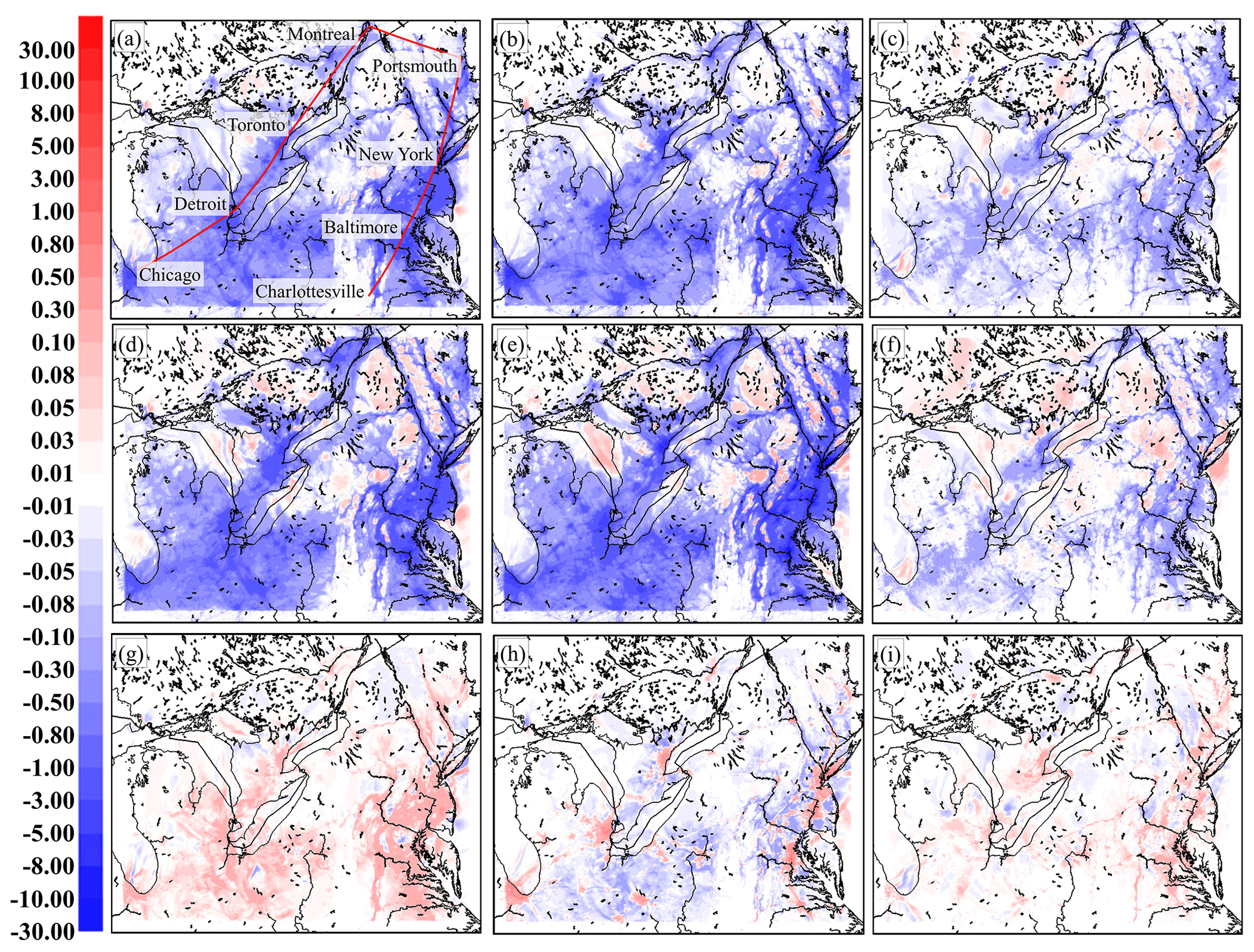
Figure 10Difference in 30 d average surface NO2, PM2.5, and O3, January 2016, in the Pan Am 2.5 km grid cell size domain simulation. Averages are paired at 10:00, 14:00, and 22:00 UTC according to species; (a–c): ΔNO2; (ppbv) (d–f) ΔPM2.5 (µg m−3); (g–i) ΔO3 (ppbv). Red line in (a) indicates the position of the vertical cross section shown in Fig. 11.
UTC hour average differences between the two 2.5 km grid cell size simulations, for the three species evaluated for the summer and winter simulations, appear in Figs. S6 and S8 and 10 and 12, respectively. The summer differences in surface concentration (Fig. S6) are the largest at 06:00 local time (10:00 UTC; first column of panels) and have largely decreased to near zero by 18:00 (22:00 UTC; last column). Corresponding concentration vertical distribution differences along a cross section linking the major cities show the early morning depletion (increase) of NO2; PM2.5 (O3) is coupled to increases (decreases) aloft (Fig. S7, first column of panels). NO2 and PM2.5 reductions extend to altitudes of up to 2 km with the increase in radiatively driven turbulence during the day, while the change in NOx to volatile organic compound (VOC) ratio regime aloft leads to increases in lower-troposphere O3 (Fig. S7, second column). Daytime mixing increases lead to a reduction in the effect by nightfall (Fig. S7, third column). VIT-enhanced transport of NO2 from urban to rural areas can also be seen (Fig. S6, first row, compare panels a, b, c; note increases in NO2 on the periphery of the urban areas, pink to red colors). This additional NOx added to NOx-limited regions leads to low-level (mostly sub-ppbv) increases in daytime O3 at 10:00 which persist through to 18:00. Over the Great Lakes, the change in vertical transport on land, coupled with daytime lake breeze circulation (Makar et al., 2010; Joe et al., 2018; Stroud et al., 2020), results in a decrease in daytime NO2 and PM2.5 over the lakes and corresponding late-afternoon O3 increases (Fig. S6, blue colors in center column of panels over the lakes for NO2 and PM2.5, red colors in the final panel of the sequence for O3). The changes in the near-roadway environment thus have larger regional effects, changing the pathway and reaction chemistry of transported chemicals on a regional scale.
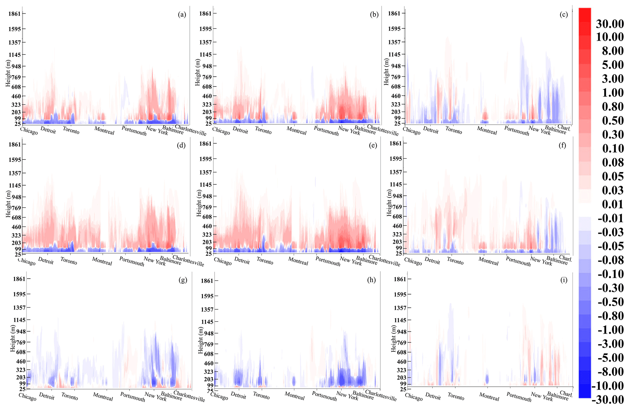
Figure 11Vertical cross sections of concentration differences between major eastern North American cities, January 2016; panels arranged as in Fig. 10. Vertical coordinate: unitless hybrid, the top of the scale is approximately 2 km. Units: ΔNO2, ΔO3 – ppbv; ΔPM2.5 – µg m−3.
The stronger impact of VIT under winter conditions is illustrated in Figs. 10 and 11; NO2 decreases (Figs. 10 and 11a–c) persist throughout the day, although to a lower degree by 18:00 (contrast Figs. S6 and S7a–c to Figs. 10 and 11a–c). The vertical influence of VIT reaches an altitude of approximately 2 km in the winter (1 km in the summer); contrast Figs. S7 and 11. The absence of winter biogenic hydrocarbon production during the day has likely limited the daytime increase in O3 to the cities (compare Fig. S6h with Fig. 10h). The large effect of VIT along major roadways can be seen in both Figs. S6 and 10, particularly in the 06:00 column of panels a, d, and g in both figures, with the greatest reductions aside from urban regions occurring along major roadways (e.g., Chicago to Detroit area).
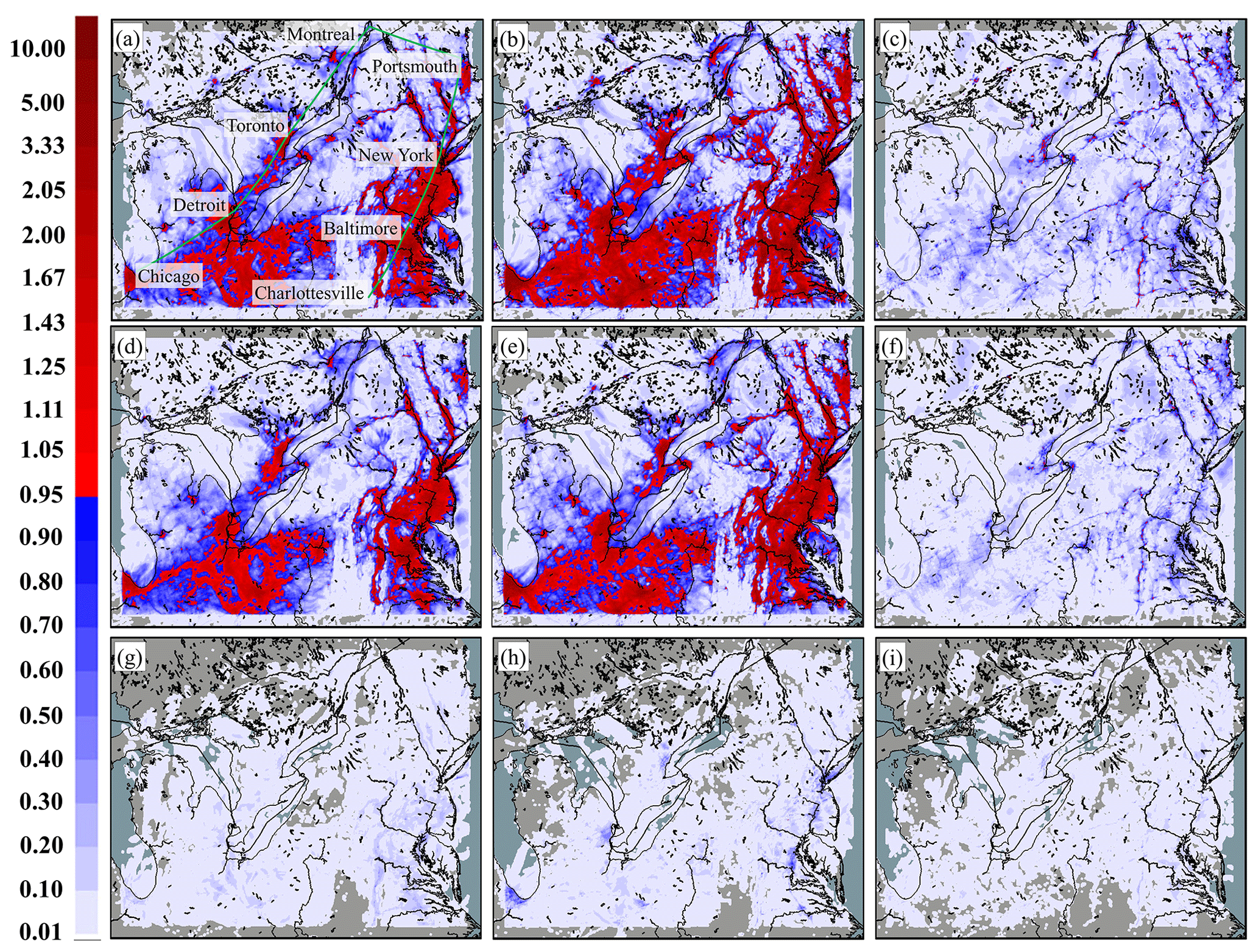
Figure 12The 90 % confidence ratio values (see Eq. 14) for the 30 d average surface NO2, PM2.5, and O3, January 2016, in the Pan Am 2.5 km grid cell size domain simulation. Panels arranged as in Fig. 10: (10:00, 14:00, and 22:00 UTC) according to species: (a–c) NO2; (d–f) PM2.5; (g–i) O3 (ppbv). Green line in (a) indicates the position of the vertical cross section shown in Fig. 13. Values>1.0 (red colors) indicate that the simulations differ at greater than 90 % confidence.

Figure 13Vertical cross sections of 90 % confidence ratio values (see Eq. 14) between major eastern North American cities, January 2016; panels arranged as in Fig. 10. Values>1.0 (red colors) indicate that the simulations differ at greater than 90 % confidence.
The spatial extent of the region where the wintertime mean values for the Pan Am domain differ at greater than 90 % confidence are shown in Figs. 12 and 13 for the model's surface concentrations and the corresponding vertical cross section, respectively. The corresponding summertime differences for this domain are shown in Figs. S8 and S9. For the wintertime Pan Am domain simulations, surface NO2 and PM2.5 >90 % confidence ratio regions are similar to those of the continental 10 km domain and can be seen to extend into the late morning hours (14:00 UTC; 10:00 local time; Fig. 12b and e). The mean values of NO2 and to a lesser extent PM2.5 also differ at greater than 90 % confidence later in the day in the urban core regions (Fig. 12c and f). In contrast to the continental-scale results (Fig. 8) the influence of VIT on surface O3 approaches but remains below the 90 % confidence level at 14:00 UTC in the urban regions (Fig. 12h) and remains below 90 % confidence at the other times shown. The vertical influence of wintertime VIT results in mean values differing at greater than 90 % confidence up to ∼700 m altitude for NO2 and PM2.5, and the above-ground O3 mean values differ at greater than 90 % confidence for regions between 25 and 200 m altitude over specific large urban areas (e.g., New York City at 14:00 UTC, Fig. 13h). Regions of greater than 90 % confidence in the vertical at 22:00 UTC for NO2 and PM2.5 are confined to the urban core regions near the surface (Fig. 13c and f). For the summertime high-resolution Pan Am domain simulations, differences at greater than 90 % confidence occur for surface NO2 and PM2.5 at night and in the early morning (Figs. S8 and S9a and d) and persist until the later morning over parts of the Great Lakes (Fig. S8b and e) and isolated locations over cities (Fig. S9b and e). Differences in the mean ozone aloft occur at night at greater than 90 % confidence over the largest cities (e.g., New York, Fig. S9a).
Taken together, Figs. 8, 12, 13, S8, and S9 show that the incorporation of VIT into the model results in mean values which are statistically different at greater than 90 % confidence (red areas, for these figures) for NO2 and PM2.5 over large regions and to a lesser degree for O3 over urban areas, with a greater influence at night, in the early morning, and under the more stable conditions of winter compared to summer.
Differences in station-specific performance scores for the two simulations for the 2.5 km grid cell size domain, constructed as for the 10 km domain, are shown in Figs. S10–S12 (summer) and S13–S15 (winter) for NO2, PM2.5, and O3.
The summer scores (Figs. S10–S12) show the most significant improvements in the urban areas across all performance metrics, with the largest relative magnitude differences for NO2 and PM2.5 and lower magnitude changes for O3. As for the North American simulations, O3 performance improvements occur in the cities, due to increased vertical mixing, and O3 scores in rural regions have degraded but may be improved with the use of a forest canopy parameterization, as discussed further in the Supplement (Figs. S5 and related text, S12, and S15). The overall impact of the incorporation of the VIT parameterization is clearly a positive one, particularly in urban areas: VIT has been shown to have a significant impact on summertime urban and suburban-scale photochemistry.
The metrics of the winter 2.5 km station-specific evaluation for NO2 (Fig. S13) show both local improvements and degradation in performance, depending on location. Wintertime PM2.5 performance improves substantially across most metrics and most locations (Fig. S14). Wintertime ozone performance is variable, although improvements can be seen for most metrics within the largest urban areas (Fig. S15).
Our work implies that the turbulence associated with vehicle motion is capable of having a significant effect on the concentrations of key pollutants in the lower atmosphere, using a parameterization which allows these effects to be incorporated at the relatively coarse horizontal resolutions of regional chemical transport models. Incorporating that effect into both continental-scale and higher-resolution regional-/urban-scale air implementations of a pollution model resulted in an overall improvement in model performance, across several different performance metrics. The improvement at higher resolution (when the TEB urban parameterization was included in the model setup) implies that the mixing associated with urban radiative transfer and roughness is not sufficient to account for the observed pollutant concentrations; the effect of VIT is robust despite differences in radiative transfer schemes and across different horizontal resolutions.
However, we also acknowledge several limitations of our VIT formulation and have recommendations for future work which would allow it to be improved and the uncertainties in our analysis reduced.
First, we have assumed that single-vehicle-induced turbulence accounts for all of the turbulent kinetic energy contributed by vehicles (Gordon et al., 2012; Miller et al., 2018). The passage of multiple vehicles also induces a “wake flow” in their direction of motion. While this effect has been recognized in very high-resolution roadway-scale models (Eskridge and Catalano, 1987; Eskridge et al., 1991), the breakdown of opposing wake flows into turbulence (arising from two-way traffic and/or multiple lanes of traffic traveling at different speeds) has not been examined, to the best of our knowledge. However, these wake flows are of sufficiently high energy that their residual power is being harnessed via vertical-turbine wind power generation systems in both Turkey (Devecitech, 2020) and Scotland (Shell, 2020). The single-vehicle additive parameterization we have created here may thus underestimate the net turbulent effect of vehicle passage. At the same time, our assumption that individual VIT within a grid cell is simply additive may also be incorrect, resulting in overestimates of that portion of the net VIT. With the advent of Doppler lidar systems with sufficient time resolution to capture turbulence, we advocate for and are currently embarking on new observation studies employing these systems in scan mode across highways, to fully characterize all vehicle-induced contributions to turbulence as a function of the number and type of vehicles crossing below a lidar scan path perpendicular to the highway.
Second, our assumption that each vehicle's pathway crosses the grid cell is a considerable source of uncertainty. There we are limited by the lack of availability of simultaneous vehicle speed and number data. However, recent developments in satellite-based radar technology have been shown to provide accurate estimates of the speed of individual vehicles along major highways (Meyer et al., 2006; Bethke et al., 2006), and binning and collection of these data may improve the linkage between the more commonly available vehicle-kilometer-traveled data and VIT beyond that used here. Other sources of gridded vehicle and/or road density data (World Bank, 2018) should also be explored.
Third, one consideration for our parameterization is the issue of “traffic jams”; a large number of vehicles being present on the road without much motion in such conditions. However, we note that in this case, the number of vehicles crossing a point in space will drop – that is, if the underlying traffic data (vehicle kilometer traveled) are of sufficient quality that traffic jams are included, the existing parameterization should adequately handle these effects. Both our second and this third consideration argue for the creation of more accurate vehicle travel data for use in air-quality models.
Last, we note that the ambient concentrations of pollutants such as NO2, O3, and PM2.5 are influenced by a host of factors included in other parameterizations of air-quality models and in the quality of the available emissions data. However, we have shown here that improvements in the forecast quality of three different species with human-health impacts may be achieved through the same process improvement. An examination of all of the other possible sources of error in air-quality models is beyond the scope of this work. This work is not intended to be taken as a review or critique of existing boundary layer parameterizations within meteorological or regional air-quality models. There has been excellent work in recent years on improving these parameterizations, and there are several reviews discussing this topic in the literature (e.g., Edwards et al., 2020). Rather, we focus here on an ancillary problem specific to regional air-quality models: whether the turbulent kinetic energy associated with vehicle motion could account for sufficient sub-grid-scale vertical mixing to influence the concentrations of fresh surface-emitted pollutants at and above roadways and further downwind, that is, on the extent to which the at-source vertical transport of fresh pollutants from the mobile sector needs to take into account local sources of energy for transport at the point of emission (whether in large stacks – Gordon et al., 2018, Akingunola et al., 2018 – or over roadways, as examined here).
Despite the uncertainties identified above, our analysis has shown the following:
-
The drop-off of VIT with height above moving vehicles is well-represented by a Gaussian distribution, from multiple measurement and computational fluid dynamics modeling studies.
-
The mixing lengths inferred from these studies ranges from 2.50 m (for individual isolated cars) through ∼10 m (vehicle ensembles) to 41 m (vehicle ensembles in a street canyon environment). We also note that the gradient in the net thermal turbulent transfer coefficients drives concentration changes due to VIT. The expectation that VIT is capable of vertical transport out of the lowest layers of a regional model is therefore a reasonable one.
-
The magnitude of the localized energy input from VIT, while smaller than the input of solar energy during daylight hours, is equivalent in magnitude to the energy perturbations resulting from the use of a state-of-the-art urban radiative balance model (TEB; see Methodology section). That is, locally, VIT has sufficient energy to be equivalent to the impact of an improved urban radiative transfer scheme – underlining its importance for vertical transport of pollutants.
-
The impact of VIT depends on both local traffic conditions and the background meteorological conditions, with the maximum effect occurring when turbulence in the ambient atmosphere is relatively weak (night through early morning) and traffic levels are relatively high (morning rush hour).
-
The use of the VIT parameterization has been demonstrated to result in decreases in air-quality model error across three different key pollutants, with the most striking results for mean biases, without resorting to the use of imposed minima in the thermal turbulent exchange coefficients frequently used in air-quality models. These differences occur at greater than 90 % confidence over much of the model domains for NO2 and PM2.5 and in urban core regions for O3 at 10 km resolution as well as up to hundreds of meters above the surface.
-
VIT has a significant impact on the rapid vertical distribution of freshly emitted pollutants on the very localized scale of roadways where the enhanced mixing occurs, in analogy to the rapid vertical transport used in parameterizations of plume rise from large stacks. Its impact on mixing of pre-existing meteorological and chemical variables on the grid cell scale is expected to be small.
Based on these findings, we conclude that VIT has a significant impact on pollutant transport and dispersion out of the lowest layer of the atmosphere and recommend its inclusion in regional air-quality models. Further improvements to the parameterizations found herein would result from additional observations of TKE using Doppler lidar techniques of vehicle ensembles under realistic driving conditions.
The data sets used here for model evaluation are available from the publicly accessible websites of the AQS network at https://www.epa.gov/aqs (last access: 21 July 2021, US EPA, 2021) and the NAPS network at http://maps-cartes.ec.gc.ca/ rnspa-naps/data.aspx (last access: 21 July 2021, Government of Canada, 2021).
The supplement related to this article is available online at: https://doi.org/10.5194/acp-21-12291-2021-supplement.
PAM was responsible for the theoretical development of the VIT parameterization, initial coding, study design, and writing of paper drafts. CS, SR, and PC provided assistance with Pan Am domain simulations and analysis. AA was responsible for final code versions and assistance with North American domain simulations and analysis. JZ and QZ provided emissions processing assistance and the generation of vehicle-kilometer-traveled fields for both North American and Pan Am domains. CS, AA, and JZ also provided comments and advice on subsequent paper drafts and responses to reviewers.
The authors declare that they have no conflict of interest.
Publisher's note: Copernicus Publications remains neutral with regard to jurisdictional claims in published maps and institutional affiliations.
The authors would like to acknowledge the contract assistance of Elisa Boutzis under the direction of Junhua Zhang in the generation of VKT gridded fields.
This paper was edited by Ronald Cohen and reviewed by two anonymous referees.
Abelsohn, A. and Steib, D. M.: Health effects of outdoor air pollution: approach to counseling patients using the Air Quality Health Index, Can. Fam. Physician, 57, 881–887, 2011.
Adelman, Z., Baek, B. H., Brandmeyer, J., Seppanen, C., Naess, B., and Yang, D.: Spatial Surrogate Development for 2014 Emissions Modeling Platforms, 2017 International Emissions Inventory Conference, 14–18 August, Baltimore, MD, USA, available at: https://www.epa.gov/sites/production/files/2017-11/documents/surrogate_developement.pdf (last access: 21 July 2021), 2017.
Akingunola, A., Makar, P. A., Zhang, J., Darlington, A., Li, S.-M., Gordon, M., Moran, M. D., and Zheng, Q.: A chemical transport model study of plume-rise and particle size distribution for the Athabasca oil sands, Atmos. Chem. Phys., 18, 8667–8688, https://doi.org/10.5194/acp-18-8667-2018, 2018.
Bethke, K.-H., Baumgartner, S., Gabele, M., Hounam, D., Kemptner, E., Klement, E., Krieger, G., and Erxleben, R.: Air- and spaceborne monitoring of road traffic using SAR moving target indication – Project TRAMRAD, ISPRS J. Photogramm., 61, 243–259, 2006.
Bou-Zeid, E., Meneveau, C., and Parlange, M. B.: Large-eddy simulation of neutral atmospheric boundary layer flow over heterogeneous surfaces: Blending height and effective surface roughness, Water Resour. Res., 40, W02505, https://doi.org/10.1029/2003WR002475, 2004.
Bradshaw, P.: Possible origin of Prandt's mixing-length theory, Nature, 249, 135–136, https://doi.org/10.1038/249135b0, 1974.
Briggs, G. A.: Plume Rise Predictions, Chapter 3, in: Lectures on Air Pollution and Environmental Impact Analysis, edited by: Huagen, D. A., American Meteorological Society, Boston, MA, USA, 59–111, https://doi.org/10.1007/978-1-935704-23-2, 1982.
Briggs, G. A.: Plume rise and buoyancy effects, atmospheric sciences and power production, in: DOE/TIC-27601 (DE84005177), edited by: Randerson, D., TN. Technical Information Center, US Dept. of Energy, Oak Ridge, USA, 327–366, 1984.
Caron, J-F., Milewski, T., Buehner, M., Fillion, L., Reszka, M., Macpherson, S., and St-James, J.: Implementation of deterministic weather forecasting systems based on ensemble-variational data assimilation at Environment Canada. Part II: The regional system, Mon. Weather Rev., 143, 2560–2580, https://doi.org/10.1175/MWR-D-14-00353.1, 2015.
Chen, J. and GEM-MACH development team: GEM-MACH atmospheric chemistry module for the GEM numerical weather pre-diction model, Environment and Climate Change Canada, Zenodo, https://doi.org/10.5281/zenodo.2579386 (last access: 3 March 2020), 2019.
Cote, J. C., Desmarais, J.-G., Gravel, G., Methot, A., and Patoine, A.: The operational CMC- MRB Global Environmental Multiscale (GEM) Model. Part II: results, Mon. Weather Rev., 126, 1397–1418, 1998a.
Cote, J. C., Gravel, S., Methot, A., Patoine, A., Roch, M., and Staniforth, A.: The operational CMC-MRB Global Environmental Multiscale (GEM) Model. Part I: design considerations and formulation, Mon. Weather Rev., 126, 1373–1395, 1998b.
Devecitech: Devecitech: Tech of the future, available at: https://devecitech.com/?page_id=5, last access: 21 February 2020.
Di Sabatino, S., Kastner-Klein, P., Berkowicz, R., Britter, R. E., and Fedorovich, E.: The modeling of turbulence from traffic in urban dispersion models – Part I: Theoretical considerations, Environ. Fluid Mech., 3, 129–143, 2003.
Edwards, J. M., Meljaars, A. C. M., Holtslag, A. A. M., and Lock, A. P.: Representation of boundary-layer processes in numerical weather prediction and climate models, Bound.-Lay. Meteorol., 177, 511–539, https://doi.org/10.007/s10546-020-00530-z, 2020.
EPA: Data from US EPA, available at: ftp://newftp.epa.gov/air/emismod/2011/v3platform/2017emissions/2017ek_cb6v2_v6_11g_inputs_onroad.zip (last access: 3 March 2020), 2017.
Eskridge, R. E. and Catalano, J. A.: ROADWAY – a numerical model for predicting air pollutants near highways, Users Guide, US EPA, 134 pp., available at: https://nepis.epa.gov/Exe/ZyPDF.cgi/20015RHA.PDF?Dockey=20015RHA.PDF (last access: 25 February 2020), 1987.
Eskridge, R. E., Petersen, W. B., and Rao, S. T.: Turbulent diffusion behind vehicles: effect of traffic speed on pollutant concentrations, JAPCA J. Air Waste Ma., 41, 312–317, https://doi.org/10.1080/10473289.1991.10466848, 1991.
Galmarini, S., Hogrefe, C., Brunner, D., Makar, P. A., Baklanov, A.: Preface, Atmos. Environ., 115, 340–344, 2015.
Gordon, M., Staebler, R. M., Liggio, J., Makar, P. A., Li, S.-M., Wentzell, J., Lu, G., Lee, P., and Brook, J. R.: Measurements of enhanced turbulent mixing near highways, J. Appl. Meteorol. Clim., 51, 1618–1632, 2012.
Gordon, M., Makar, P. A., Staebler, R. M., Zhang, J., Akingunola, A., Gong, W., and Li, S.-M.: A comparison of plume rise algorithms to stack plume measurements in the Athabasca oil sands, Atmos. Chem. Phys., 18, 14695–14714, https://doi.org/10.5194/acp-18-14695-2018, 2018.
Government of Canada: National Air Pollution Surveillance (NAPS) Program, Government of Canada Open Data Portal [data set], available at: http://maps-cartes.ec.gc.ca/ rnspa-naps/data.aspx, last access: 21 July 2021.
Hu, X.-M., Klein, P. M., and Xue, M.: Evaluation of the updated YSU Planetary Boundary Layer Scheme within WRF for Wind Resource and Air Quality Assessments, J. Geophys. Res.-Atmos., 118, 10490–10505, https://doi.org/10.1002/jgrd.50823, 2013.
Joe, P., Belair, S., Ber Nier, N. B., Bouchet, V., Brook, J. R., Brunet, D., Burrows, W., Charland, J.-P., Dehghan, A., Driedger, N., Duhamie, C., Evans, G., Filion, A.-B., Frenette, R., DeGrandpre, J., Gultepe, I., Henderson, D., Herdt, A., Hilker, N., Huang, L., Hung, E., Isaac, G., Jeong, C.-H., Johnston, D., Klassen, J., Leroyer, S., Lin, H., MacDonald, M., MacPhee, J., Mariani, Z., Munoz, T., Ried, J., Robichaud, A., Rochon, Y., Shairsing, K., Sills, D., Spacek, L., Stroud, C., Su, Y., Taylor, N., Vanos, J., Voogt, J., Wang, J. M., Wiechers, T., Wren, S., Yang, H., and Yip, T.: The Environment Canada Pan and ParaPan American science showcase project, B. Am. Meteorol. Soc., 99, 921–953, https://doi.org/10.1175/BAMS-D-16-0162.1, 2018.
Kain, J. S.: The Kain–Fritsch convective parameterization: an update, J. Appl. Meteorol., 43, 170–181, 2004.
Kastner-Klein, P., Fedorovich, E., Ketzel, M., Berkowicz, R., and Britter, R.: The modelling of turbulence from traffic in urban dispersion models – Part II: Evaluation against laboratory and fullscale concentration measurements in street canyons, Environ. Fluid Mech., 3, 145–172, 2003.
Kim, S.-W., Barth, M. C., and Trainer, M., Impact of turbulent mixing on isoprene chemistry, Geophys. Res. Lett., 43, 7701–7708, 2016.
Kim, Y.: Quantification of vehicle-induced turbulence on roadways using computational fluid dynamics simulation, M.Sc. Thesis, Department of Chemical Engineering and Applied Chemistry, University of Toronto, Toronto, Ontario, Canada, 93 pp., 2011.
Kim, Y., Sartelet, K., Raut, J-C., and Chazette, P.: Influence of an urban canopy model and PBL schemes on vertical mixing for air quality modeling over Greater Paris, Atmos. Environ., 107, 289–306, 2015.
Kim, Y., Huang, L., Gong, S., Jia, C. Q.: A new approach to quantifying vehicle induced turbulence for complex traffic scenarios, Can. J. Chem. Eng., 24, 71–78, 2016.
Klein, P. M., Hu, X.-M., and Xue, M.: Impacts of mixing processes in the nocturnal atmospheric boundary layer on urban ozone concentrations, Bound.-Lay. Meteorol., 150, 107–130, 2014.
Lemonsu, A., Belair, S., Mailhot, J., and Leroyer, S.: Evaluation of the Town Energy Balance model in cold and snowy conditions during the Montreal urban snow experiment, 2005, J. Appl. Meteorol. Clim., 49, 346–362, 2010.
Leroyer, S., Belair, S., Husain, S. Z., and Mailhot, J.: Subkilometer numerical weather prediction in an urban coastal area: a case study over the Vancouver metropolitan area, J. Appl. Meteorol. Clim., 53, 1433–1453, 2014.
Li, Y., Barth, M. C., Chen, G., Patton, E. G., Kim, S.-W., Wisthaler, A., Mikoviny, T., Fried, A., Clark, R., and Steiner, A. L.: Large-eddy simulation of biogenic VOC chemistry during the DISCOVER-AQ 2011 campaign, J. Geophys. Res.-Atmos., 121, 8083–8105, 2016.
Makar, P. A., Gravel, S., Chirkov, V., Strawbridge, K. B., Froude, F., Arnold, J., and Brook, J.: Heat flux, urban properties, and regional weather, Atmos. Environ., 40, 2750–2766, https://doi.org/10.1016/j.atmosenv.2005.11.061, 2006.
Makar, P. A., Zhang, J., Gong, W., Stroud, C., Sills, D., Hayden, K. L., Brook, J., Levy, I., Mihele, C., Moran, M. D., Tarasick, D. W., He, H., and Plummer, D.: Mass tracking for chemical analysis: the causes of ozone formation in southern Ontario during BAQS-Met 2007, Atmos. Chem. Phys., 10, 11151–11173, https://doi.org/10.5194/acp-10-11151-2010, 2010.
Makar, P. A., Nissen, R., Teakles, A., Zhang, J., Zheng, Q., Moran, M. D., Yau, H., and diCenzo, C.: Turbulent transport, emissions and the role of compensating errors in chemical transport models, Geosci. Model Dev., 7, 1001–1024, https://doi.org/10.5194/gmd-7-1001-2014, 2014.
Makar, P. A., Gong, W., Hogrefe, C., Zhang, Y., Curci, G., Zabkar, R., Milbrandt, J., Im, U., Balzarini, A., Baro, R., Bianconi, R., Cheung, P., Forkel, R., Gravel, S., Hirtl, H., Honzak, L., Hou, A., Jimenz-Guerrero, P., Langer, M., Moran, M. D., Pabla, B., Perez, J. L., Pirovano, G., San Jose, R., Tuccella, P., Werhahn, J., Zhang, J., and Galmarini, S.: Feedbacks between air pollution and weather, part 2: Effects on chemistry, Atmos. Environ., 115, 499–526, 2015a.
Makar, P. A., Gong, W., Milbrandt, J., Hogrefe, C., Zhang, Y., Curci, G., Zabkar, R., Im, U., Balzarini, A., Baro, R., Bianconi, R., Cheung, P., Forkel, R., Gravel, S., Hirtl, H., Honzak, L., Hou, A., Jimenz-Guerrero, P., Langer, M., Moran, M. D., Pabla, B., Perez, J. L., Pirovano, G., San Jose, R., Tuccella, P., Werhahn, J., Zhang, J., and Galmarini, S.: Feedbacks between air pollution and weather, part 1: Effects on weather, Atmos. Environ., 115, 442–469, 2015b.
Makar, P. A., Staebler, R. M., Akingunola, A., Zhang, J., McLinden, C., Kharol, S. K., Pabla, B., Cheung, P., and Zheng, Q.: The effects of forest canopy shading and turbulence on boundary layer ozone, Nat. Commun., 8, 15243, https://doi.org/10.1038/ncomms15243, 2017.
Mason, V.: A physically-based scheme for the urban energy balance in atmospheric models, Bound.-Lay. Meteorol., 94, 357–397, 2000.
Mensink, C., Lefebre, F., Janssen, L., and Cornelis, J.: A comparison of three street canyon models with measurements at an urban station in Antwerp, Belgium, Environ. Modell. Softw., 21, 514–516, 2014.
Meyer, F., Hinz, S., Laika, A., Weihing, D., and Bamler, R.: Performance analysis of the TerraSAR-X Traffic monitoring concept, ISPRS J. Photogramm., 61, 225–242, 2006.
Milbrandt, J. A., Bélair, S., Faucher, M., Vallée, M., Carrera, M. L., and Glazer, A.: The pan-Canadian High Resolution (2.5 km) Deterministic Prediction System, Weather Forecast., 31, 1791–1816, 2016.
Miller, S. J., Gordon, M., Staebler, R. M., and Taylor, P. A.: A study of the spatial variation of vehicle-induced turbulence on highways using measurements from a mobile platform, Bound.-Lay. Meteorol., 171, 1–29, https://doi.org/10.1007/s10546-018-0416-9, 2018.
Moran M. D., Ménard, S., Talbot, D., Huang, P., Makar, P. A., Gong, W., Landry, H., Gravel, S., Gong, S., Crevier, L.-P., Kallaur, A., and Sassi, M.: Particulate-matter forecasting with GEM-MACH15, a new Canadian air-quality forecast model, in: Air Pollution Modelling and Its Application XX, edited by: Steyn, D. G. and Rao, S. T., Springer, Dordrecht, 289–292, 2010.
Moran, M. D., Lupu, A., Zhang, J., Savic-Jovcic, V., and Gravel, S.: A comprehensive performance evaluation of the next generation of the Canadian operational regional air quality deterministic prediction system, Springer Proceedings in Complexity, Cham, Switzerland, Cham, Switzerland, 75–81, 2018.
Ouwersloot, H. G., Vilà-Guerau de Arellano, J., van Heerwaarden, C. C., Ganzeveld, L. N., Krol, M. C., and Lelieveld, J.: On the segregation of chemical species in a clear boundary layer over heterogeneous land surfaces, Atmos. Chem. Phys., 11, 10681–10704, https://doi.org/10.5194/acp-11-10681-2011, 2011.
Prandtl, L.Z., Bericht über Untersuchungen zur ausgebildeten Turbulenz, J. Appl. Math. Mech., 5, 136–139, https://doi.org/10.1002/zamm.19250050212, 1925.
Rao, K. S., Gunter, R. L., White, J. R., and Hosker, R. P.: Turbulence and dispersion modeling near highways, Atmos. Environ., 36, 4337–4346, 2002.
Rao, S. T., Sedefian, L., and Czapksi, U. H.: Characteristics of turbulence and dispersion of pollutants near major highways, J. Appl. Meteorol., 18, 286–293, 1979.
Ren, S., Stroud, C., Belair, S., Leroyer, S., Moran, M., Zhang, J., Akingunola, A., and Makar, P.: Impact of Urban Land Use and Anthropogenic Heat on Air Quality in Urban Environments, in: Air Pollution Modeling and its Application XXVI, ITM 2018, edited by: Mensink, C., Gong, W., and Hakami, A., Springer Proceedings in Complexity, Springer, Cham, Switzerland, 153–158, https://doi.org/10.1007/978-3-030-22055-6_24, 2020.
Shell: Winds of Change: Turbine Turns Traffic Into Energy, available at: https://www.shell.com/inside-energy/turbine-turns-traffic-into-energy.html, last access: 21 February 2020.
Stieb, D. M., Burnett, R. T., Smith-Doiron, M., Brion, O., Hwashin, H. S., and Economou, V.: A new multipollutant, no-threshold air quality health index based on short-term associations observed in daily time-series analyses, JAPCA J. Air Waste Ma., 58, 435–450, 2008.
Stroud, C., Ren, S., Zhang, J., Moran, M., Akingunola, A., Makar, P. A., Munoz-Alpizar, R., Leroyer, S., Bélair, S., Sills, D., and Brook, J. R.: Chemical analysis of surface-level ozone exceedances during the 2015 pan American games, Atmosphere, 11, 572, https://doi.org/10.3390/atmos11060572, 2020.
US EPA: Air Quality System (AQS), available at: https://www.epa.gov/aqs, last access: 21 July 2021.
Woodward, H., Stettler, M., Pavlidis, D., Aristodemou, E., ApSimon, H., and Pain, C.: A large eddy simulation of the dispersion of traffic emissions by moving vehicles at an intersection, Atmos. Environ., 215, 116891, https://doi.org/10.1016/j.atmosenv.2019.116891, 2019.
World Bank: GRIP (Global Roads Inventory Dataset) – 2018: Road Density, available at: https://datacatalog.worldbank.org/dataset/grip-global-roads-inventory-dataset-2018-road-density (last access: 21 February 2020), 2018.
Vinuesa, J.-F. and Vilà-Guerau de Arellano, J.: Introducing effective reaction rates to account for inefficient mixing of the convective boundary layer, Atmos. Environ., 39, 445–461, 2005.
Zhang, Y., Gu, Z., and Yu, C. W.: Large eddy simulation of vehicle induced turbulence in an urban street canyon with a new dynamically vehicle-tracking scheme, Aerosol Air Qual. Res., 17, 865–874, https://doi.org/10.4209/aaqr.2016.05.0204, 2017.