the Creative Commons Attribution 4.0 License.
the Creative Commons Attribution 4.0 License.
 | 09 Aug 2021
Towards kilometer-scale ocean–atmosphere–wave coupled forecast: a case study on a Mediterranean heavy precipitation event
Cindy Lebeaupin Brossier
Marie-Noëlle Bouin
The western Mediterranean Sea area is frequently affected in autumn by heavy precipitation events (HPEs). These severe meteorological episodes, characterized by strong offshore low-level winds and heavy rain in a short period of time, can lead to severe flooding and wave-submersion events. This study aims to progress towards an integrated short-range forecast system via coupled modeling for a better representation of the processes at the air–sea interface. In order to identify and quantify the coupling impacts, coupled ocean–atmosphere–wave simulations were performed for a HPE that occurred between 12 and 14 October 2016 in the south of France. The experiment using the coupled AROME-NEMO-WaveWatchIII system was notably compared to atmosphere-only, coupled atmosphere–wave and ocean–atmosphere simulations. The results showed that the HPE fine-scale forecast is sensitive to both couplings: the interactive coupling with the ocean leads to significant changes in the heat and moisture supply of the HPE that intensify the convective systems, while coupling with a wave model mainly leads to changes in the low-level dynamics, affecting the location of the convergence that triggers convection over the sea.
Result analysis of this first case study with the AROME-NEMO-WaveWatchIII system does not clearly show major changes in the forecasts with coupling and highlights some attention points to follow (ocean initialization notably). Nonetheless, it illustrates the higher realism and potential benefits of kilometer-scale coupled numerical weather prediction systems, in particular in the case of severe weather events over the sea and/or in coastal areas, and shows their affordability to confidently progress towards operational coupled forecasts.
- Article
(14909 KB) - Full-text XML
- BibTeX
- EndNote


In the last decade, improving the forecast of intense weather events involving air–sea interactions has motivated operational forecast centers to develop and operate ocean–atmosphere–wave coupled modeling platforms for short- and medium-range weather predictions (see, for instance, the Geophysical Fluid Dynamics Laboratory (GFDL) model used at the National Weather Service, Bender et al., 2007, the Coupled Ocean/Atmosphere Mesoscale Prediction System for Tropical Cyclones (COAMPS-TC) operated at the Naval Research Laboratory for hurricane prediction, Doyle et al., 2014, the global ocean–ice–atmosphere coupled prediction system run at Environment and Climate Change Canada, Smith et al., 2018, and the recent developments at the European Centre for Medium-Range Weather Forecasts, Magnusson et al., 2019).
Tropical cyclones (TCs) above all have been known for long to be impacted by the surface cooling of the ocean they generate (e.g., Bender et al., 1993; Bender and Ginis, 2000; Bao et al., 2000). Realistic simulations have shown that the initial state of the ocean, namely, the sea surface temperature (SST) and stratification, may significantly reduce the TC intensity (e.g., Chan et al., 2001). Several large-scale studies have shown that using ocean–atmosphere coupling improves in a statistical way the prediction of TCs with respect to atmosphere-only simulations in every cyclonic basin (e.g., Bender et al., 2007; Samson et al., 2014; Mogensen et al., 2017; Lengaigne et al., 2018). Using 3D ocean models in coupled configurations is mandatory to accurately represent the complex subsurface processes (e.g., upwelling) responsible for the SST cooling (Yablonsky and Ginis, 2009). As TC development is known to be sensitive to both enthalpy and momentum transfer coefficients (Emanuel, 1986), taking into account the wave impact on the sea surface roughness can also influence the TC representation in numerical models. Case studies using ocean–atmosphere–wave coupled configurations showed an influence of wave growth on the TC intensity and development (e.g., Olabarrieta et al., 2012; Lee and Chen, 2012; Doyle et al., 2014; Pianezze et al., 2018). Sensitivity tests using representation of the surface fluxes including the impact of sea spray showed more contrasted results, depending on the parameterization used and on the case studied (e.g., Wang et al., 2001; Gall et al., 2008; Green and Zhang, 2013; Zweers et al., 2015). Most of the coupled configurations used for improving the TC forecast have horizontal resolutions of 10–25 km, enabling them to cover large oceanic basins and fine enough to properly represent relatively large-scale events like TCs. Only recent case studies make use of kilometric horizontal resolutions permitting us to simulate more accurately the fine-scale processes within the TC structure (e.g., Lee and Chen, 2012; Green and Zhang, 2013; Pianezze et al., 2018).
Extreme events also often occur in the Mediterranean Sea. For instance, medicanes are severe storms looking like TCs in their developed phase, although smaller in size and weaker (e.g., Lionello et al., 2003; Renault et al., 2012; Ricchi et al., 2017; Varlas et al., 2018, 2020; Bouin and Lebeaupin Brossier, 2020b). In medicanes as in tropical cyclones, ocean surface cooling is observed, primarily affecting the heat and moisture exchanges. Case studies based on coupled simulations gave contrasting results on the impact of the feedback from the waves or the ocean on medicanes. For instance, Ricchi et al. (2017) investigating the medicane of November 2011 using COAWST (Coupled Ocean Atmosphere–Wave Sediment Transport, Warner et al., 2010) at 5 km resolution and Bouin and Lebeaupin Brossier (2020b) studying the one occurring in November 2014 through high-resolution coupling (1.3 km for the atmosphere using MESO-NH Mesoscale Non-Hydrostatic Model – Lac et al., 2018 and 136∘ for the ocean using NEMO Nucleus for European Modelling of the Ocean – Madec and the NEMO system team, 2008) showed that the direct impact of the ocean coupling did not significantly change the track and intensity of the medicanes. Ricchi et al. (2017) suggested nevertheless that the way to calculate the sea surface roughness, and more generally the air–sea processes, can affect significantly the results by notably playing on the intensification of the near-surface wind. Also, Varlas et al. (2020) showed an overall improvement of the forecast skill over the sea using a two-way coupling between the atmosphere and waves, respectively, the WRF (Weather Research Forecasting – Skamarock et al., 2008) and WAM (the ocean WAve Model – The Wamdi Group, 1988) models.
Generally related to cyclogenesis, the Mediterranean Sea is also prone to high and local wind of continental origin, channelled and accelerated in the steep surrounding valleys, such as mistral or bora, which usually last several days and generate very rough sea states and sometimes result in strong damages (e.g., Ardhuin et al., 2007). Several case studies investigated the impact of mistral or bora wind on the ocean and the impact of using ocean–atmosphere or atmosphere–wave coupled models (e.g., Loglisci et al., 2004; Pullen et al., 2007; Small et al., 2012; Ricchi et al., 2016; Ličer et al., 2016; Seyfried et al., 2019). They showed a quick evolution of the SST and currents during this type of event, with a significant feedback on the surface heat and momentum fluxes but no significant change in the low-level atmospheric flow.
In the present study, we investigate the impact of ocean–atmosphere–wave coupling on a different kind of Mediterranean extreme weather event, namely, a heavy precipitation event (HPE, Ducrocq et al., 2014, 2016). Such events generally occur in autumn and are characterized by a large amount of precipitation over a small area in a very short time, causing huge flash floods leading to considerable damages and numerous casualties (e.g., Petrucci et al., 2019). These events are usually generated by quasi-stationary mesoscale convective systems (MCSs) fed by strong offshore low-level winds over the warm Mediterranean Sea. Air–sea processes are thus key elements in the development of those HPEs (e.g., Duffourg and Ducrocq, 2011). Rainaud et al. (2017), using the coupling between the WMED (Western Mediterranean Sea) configurations of the AROME (Application of Research to Operations at MEsoscale – Seity et al., 2011; Fourrié et al., 2015) atmosphere model at 2.5 km resolution and NEMO at a 136∘ resolution (Lebeaupin Brossier et al., 2014), reasserted the importance of an interactive ocean and its impact on the surface evaporation water supply for HPEs. In addition to this, Thévenot et al. (2016), Bouin et al. (2017), and Sauvage et al. (2020) showed the importance of taking the sea state into account in the calculation of air–sea fluxes during Mediterranean HPEs, with a significant impact on the location of the heavy precipitation. Indeed, the parameterization of sea surface turbulent fluxes is key in representing the exchanges between the different compartments. Generally implemented as bulk parameterizations (e.g., Coupled Ocean–Atmosphere Response Experiment (COARE) 3.0, Fairall et al., 2003), several formulations enable us to represent the sea state impact on the momentum and heat fluxes (Oost et al., 2002; Taylor and Yelland, 2001; Sauvage et al., 2020).

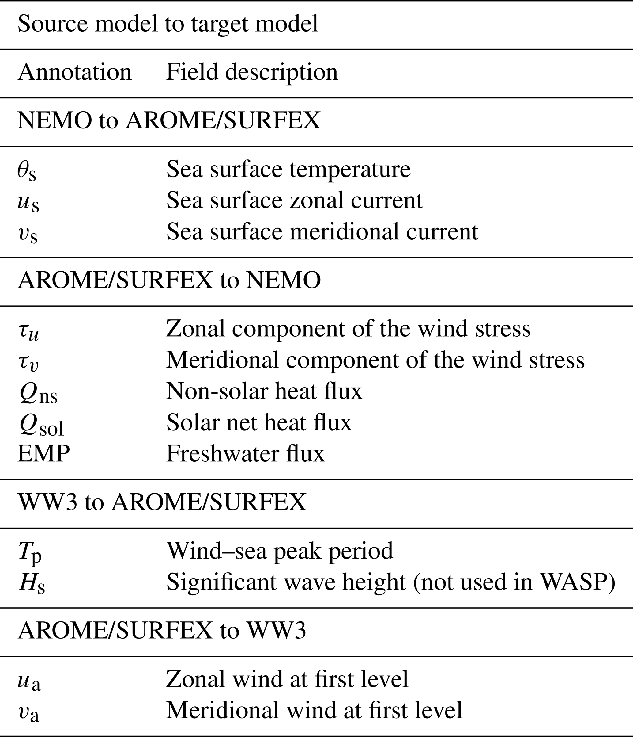
Figure 1The NEMO-AROME-WW3 coupled architecture and domains illustrated by orography (of the AROME-France domain in the SURFEX “area”) and the NWMED72 bathymetry (in the NEMO box). The SURFEX-OASIS interface (red arrows) is detailed in Voldoire et al. (2017), and the AROME-SURFEX links (green arrows) are described in Masson et al. (2013) and Seity et al. (2011). See text and Table 1 for the exchanges involving NEMO and WW3.
The studies listed above demonstrate the interest of more complete regional simulating systems in better predicting high-impact events involving air–sea interactions and combining the capabilities of fine-scale (1 to 2 km in horizontal resolution) models with ocean–atmosphere–wave coupling. Also, the continuous increase in high-performance computing capabilities fosters the development of such coupled modeling systems with kilometric resolution and makes them usable for operational forecasting (e.g., Pullen et al., 2017; Lewis et al., 2018, 2019a, b, c).
In this context, the present study describes a new kilometric regional coupled system involving the Météo-France high-resolution operational numerical weather prediction (NWP) model AROME-France, the WaveWatch III wave model (hereafter WW3, Tolman, 1992) and the NEMO ocean model, which paves the way to the future coupled regional convection-resolving NWP system of Météo-France. This system will be used here to assess the coupling impacts during an HPE which occurred from 12 to 14 October 2016.
A detailed description of the coupled system is given in Sect. 2. The main characteristics of the studied HPE and the numerical set-up are presented in Sect. 3. Then the contribution of the two-way coupled atmosphere–wave and atmosphere–ocean is analyzed in Sect. 4. In Sect. 5 the results obtained using the ocean–atmosphere–wave system are discussed. Finally, conclusions are given in Sect. 6.
This section presents the tri-coupled system that combines the ocean–atmosphere coupling previously developed between AROME and NEMO by Rainaud et al. (2017) and the wave–atmosphere interactive exchanges with the AROME-WW3 coupling as fully described by Sauvage et al. (2020). The details of the model configurations and the exchange management are given in the following for clarity purposes.
2.1 The component models
2.1.1 The atmospheric model
The non-hydrostatic AROME NWP model is used in this study, with the same forecast configuration as the one operationally used at Météo-France in 2016 (AROME-France, cy41t1, Seity et al., 2011; Brousseau et al., 2016) with a 1.3 km horizontal resolution and a domain centered over France (Fig. 1), which notably covers the northwestern Mediterranean Sea. The AROME orography is extracted from the Global 30 Arc-Second Elevation Data Set (GTOPO30) database (Gesch et al., 1999). The vertical grid has 90 hybrid η levels with a first-level thickness of almost 5 m. The time step is 50 s.
In AROME, the advection scheme is semi-Lagrangian, and the temporal scheme is semi-implicit. The 1.5-order turbulent kinetic energy scheme from Cuxart et al. (2000) is used. Due to its high resolution, the deep convection is explicitly solved in AROME, whereas the shallow convection is solved with the eddy diffusivity Kain–Fritsch (EDKF, Kain and Fritsch, 1990) parameterization. The ICE3 one-moment microphysical scheme (Pinty and Jabouille, 1998) is used to compute the evolution of five hydrometeor species (rain, snow, graupel, cloud ice and cloud liquid water). Radiative fluxes are computed with the Fouquart and Bonnel (1980) scheme for short-wave radiation and the RRTM (Rapid Radiative Transfer Model, Mlawer et al., 1997) scheme for long-wave radiation.
The surface exchanges are computed by the SURFace EXternalisé (SURFEX) surface model (Masson et al., 2013) considering four different surface types: land, towns, sea and inland waters (lakes and rivers). Output fluxes are weight-averaged inside each grid box according to the fraction of each respective tile defined with physiographic data from the ECOCLIMAP database (Masson et al., 2003) before being provided to the atmospheric model at every time step. Exchanges over land are computed using the ISBA (Interactions between Soil, Biosphere and Atmosphere) parameterization (Noilhan and Planton, 1989). The formulation from Charnock (1955) is used for inland waters, whereas the Town Energy Balance (TEB) scheme is activated over urban surfaces (Masson, 2000). The treatment of the sea surface exchanges in AROME-SURFEX is done here with the WASP (Wave-Age-dependent Stress Parameterization) scheme, detailed in Sauvage et al. (2020) and below, and the albedo is computed following the Taylor et al. (1996) scheme.
2.1.2 The ocean model
The NWMED72 configuration of the NEMO ocean model (version 3_6; Madec and the NEMO team, 2016) presented in (Sauvage et al., 2018) is used here. It covers the northwestern Mediterranean basin (Fig. 1) with a 172∘ horizontal resolution (from 1 to 1.3 km resolution) and uses 50 stretched z levels in the vertical, with a first-level thickness of 0.5 m. This configuration has two open boundaries: a southern open boundary near 38∘ N south of the Balearic Islands and Sardinia and an eastern open boundary across the Tyrrhenian Sea (12.5∘ E).
In NWMED72, the Total Variance Dissipation (TVD) scheme is used for tracer advection in order to conserve energy and enstrophy (Barnier et al., 2006). The vertical diffusion follows the standard turbulent kinetic energy formulation of NEMO (Blanke and Delecluse, 1993). In case of unstable conditions, a higher diffusivity coefficient of 10 m2 s−1 is applied (Lazar et al., 1999). The sea surface height is a prognostic variable solved thanks to the filtered free-surface scheme of Roullet and Madec (2000). A no-slip lateral boundary condition is applied, and the bottom friction is parameterized by a quadratic function with a coefficient depending on the 2D mean tidal energy (Lyard et al., 2006; Beuvier et al., 2012). The diffusion is applied along isoneutral surfaces for the tracers using a Laplacian operator with the horizontal eddy diffusivity value νh fixed at 15 m2 s−1. For the dynamics (velocity), a bi-Laplacian operator is used with the horizontal viscosity coefficient ηh fixed at 1.108 m4 s−1. The time step is 120 s.
The runoff forcing consists of daily observations for 25 French rivers around the northwestern Mediterranean Sea (see Sauvage et al., 2018, for the complete list) collected from the Banque Hydro database (hydro.eaufrance.fr) and in the monthly climatology of Ludwig et al. (2009) for the Ebro, Júcar and Tiber rivers temporally interpolated to give daily values. Each river inflow is injected in one grid point in the surface (as precipitation).
2.1.3 The wave model
The wave model is WW3 (Tolman, 1992) in version 5.16 (The WAVEWATCH III Development Group, 2016). The WW3 domain and bathymetry correspond to the NEMO-NWMED72 grid (at a 172∘ horizontal resolution), as previously presented in Sauvage et al. (2020). The time step is 60 s.
The set of parameterizations from Ardhuin et al. (2010) is used, as for most of the wave forecasting centers (Ardhuin et al., 2019). Thus, the swell dissipation is computed with the Ardhuin et al. (2009) scheme, and the wind input parameterization is from Janssen (1991). Nonlinear wave–wave interactions are computed using the discrete interaction approximation (Hasselmann et al., 1985). The parameterization of the reflection by shorelines is described in Ardhuin and Roland (2012). Moreover, the computation of the depth-induced breaking is based on the algorithm from Battjes and Janssen (1978), and the bottom friction formulation follows Ardhuin et al. (2003).
2.2 Air–sea exchanges and coupling
The coupled system AROME-NEMO-WW3 is implemented using the SURFEX-OASIS coupling interface developed by Voldoire et al. (2017). This interface permits the field exchanges between the atmospheric and ocean models on the one hand and between the atmospheric and wave models on the other hand (Fig. 1 and Table 1).
NEMO provides to the OASIS3-MCT coupler (OASIS hereafter, Craig et al., 2017) the mean SST and horizontal surface current components (us and vs) at the coupling frequency of 1 h. At the same coupling frequency, WW3 provides the peak period of the wind sea (Tp) to OASIS. These fields, after interpolation onto the AROME (SURFEX) grid, are used to compute surface fluxes at each subsequent atmospheric time step. The wind components of the first atmospheric level (ua, va) and the air–sea fluxes at the interface – namely, the solar heat flux Qsol, the non-solar heat flux Qns, the two components of the horizontal wind stress τu and τv and the atmospheric freshwater flux EMP – are computed by SURFEX and provided to OASIS, which then averages them over 1 h and interpolates and sends them to WW3 (for ua and va) or NEMO (for Qsol, Qnet, τu, τv, and EMP) at the coupling frequency. Detailed information on the different coupling namelists for each model is given in Appendix A.
The air–sea fluxes are computed taking into account near-surface atmospheric and oceanic parameters, following the radiative schemes (Fouquart and Bonnel, 1980; Mlawer et al., 1997) and the WASP turbulent flux parameterization:
where SWdown and LWdown are the incoming components of the solar and infrared radiations, respectively. θs is the SST, α is the albedo, ϵ is the emissivity and σ is the Stefan–Boltzman constant. Turbulent heat fluxes (H for sensible and LE for latent) are calculated with WASP (see the following) and thus depend on the wind speed and on the air–sea gradients of temperature and humidity, respectively, and on transfer coefficients CH and CE, respectively, which themselves depend on air stability and wave age (see the following).
The atmospheric freshwater flux is given by
where E is the evaporation, corresponding to with ℒv the vaporization heat constant. Pl and Ps are the liquid and solid surface precipitation rates (given by AROME).
The wind stress takes into account the ocean surface current (given by NEMO), as follows:
with ρa the air density, the wind at the lowest atmospheric model level (around 5 m here), the ocean surface current and u* the friction velocity. CD is the drag coefficient given by the turbulent flux parameterization.
The turbulent heat fluxes are also expressed as functions of the air–sea gradients:
with cpa the air heat capacity. Δθ and Δq represent the air–sea gradients of potential temperature (θs−θa) and specific humidity (qs−qa), respectively.
Each transfer coefficient (CX) can be expressed as
where is for wind stress, for sensible heat and for latent heat. The coefficients are a function of ψx(ζ) that describes empirically the stability, ζ is the ratio with L the Obukhov length, and z0 is the sea surface roughness length. Therefore,
and
with the subscript n referring to neutral (ζ=0) stability, z to the reference height and κ to von Karman's constant. The sea surface roughness length z0 is defined by two terms, Charnock's relation (Charnock, 1955) and a viscous contribution (Beljaars, 1994):
with ν the kinematic viscosity of dry air and the Charnock coefficient αch. In WASP, z0 depends on the wave age (χ) through the Charnock coefficient (αch), which is a power function of χ (; see Eq. (8) and Appendix A in Sauvage et al., 2020), and χ is defined as
where g is the acceleration of gravity and Tp is the peak period of waves corresponding to the wind sea, i.e., the waves generated by the local wind that are growing (χ<0.8) or in equilibrium with the wind () and that are aligned with the local wind. The reader can refer to Sauvage et al. (2020) for an enlarged description of WASP.
The AROME-France domain is more extended than the NWMED72 domain of NEMO and WW3, and as the Atlantic Ocean and the Adriatic Sea are not represented, there is no air–sea coupling in these areas: the SST comes from the AROME-France initial analysis and is constant during the run, horizontal current is considered null, and the peak period is computed inside WASP as a function of the wind speed ().
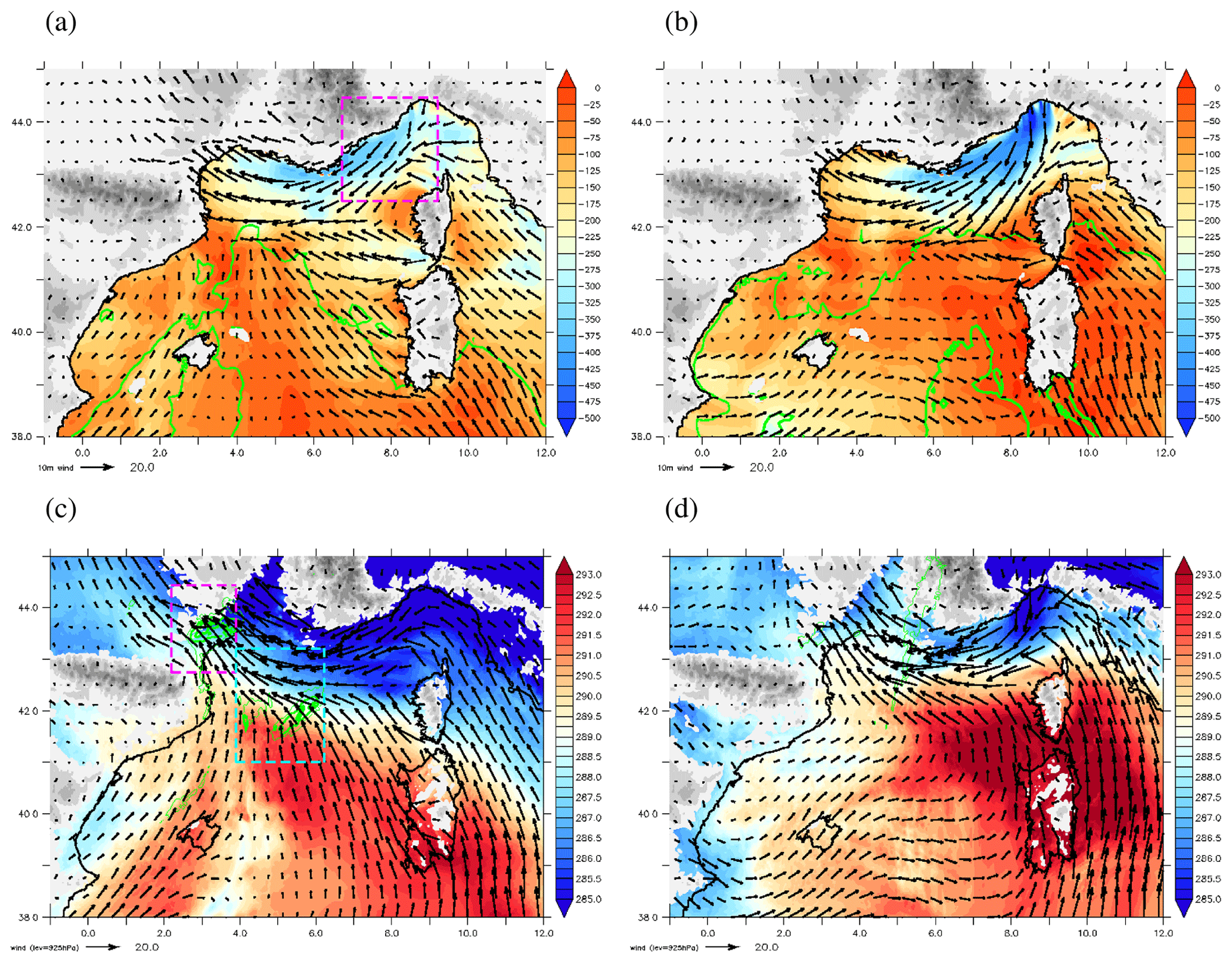
Figure 2Mean surface and atmospheric low-level conditions: (a, b) enthalpy flux over the sea (H+LE, colors, W m−2), convective available potential energy (CAPE, green contours every 750 J kg−1) and 10 m wind (arrows, m s−1) and (c, d) θw' (colors, K) and wind (arrows, m s−1) at 925 hPa and total rainfall amounts (green contours every 50 mm) from the AW forecast during (a, c) the initiation phase (Phase I, between 13 October 2016 03:00 UTC and 18:00 UTC) and (b, d) the mature phase (Phase II, between 13 October 2016 19:00 UTC and 14 October 2016 03:00 UTC). See text and Sauvage et al. (2020) for more details. The dashed purple box in (a) indicates the Azur zone. The dashed boxes in (c) indicate the Hérault (purple) and offshore (cyan) areas for precipitation analyses.
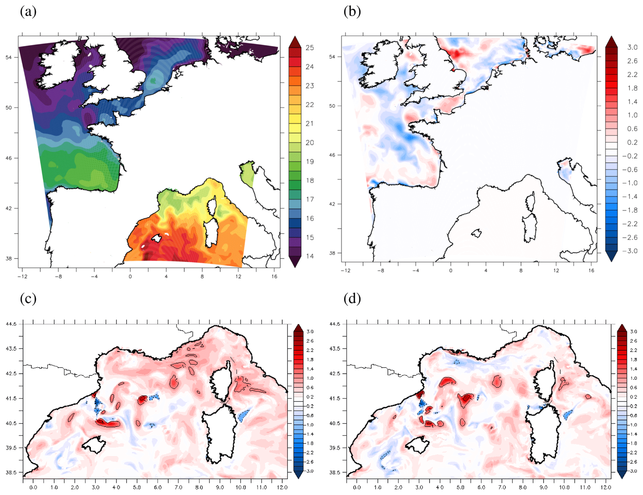
Figure 3(a) SST (∘C) forecast in AOW at 14:00 UTC on 13 October (forecast basis: 13 October 00:00 UTC) and (b) differences in initial SST fields (∘C, 13 October 00:00 UTC) between AY and AYSSTatl (AROME forecasts with persistent SST; see text and Table 2). Comparison of the AOW SST forecast (basis: 13 October 00:00 UTC) over NWM (c) at 01:00 UTC on 13 October and (d) at 00:00 UTC on 14 October, with the PSY4 daily analysis of 13 October (used in AY/AYSSTatl/AW experiments).
3.1 Case study
The HPE studied here is described in detail in Sauvage et al. (2020). Its main characteristics are briefly given in the following.
The synoptic situation of the event has been defined as a “cyclonic southerly” kind (Nuissier et al., 2011), characterized by a slow moving trough extending from the British Isles to Spain that induced at upper level a southwesterly flow over southeastern France. At low level, a cyclonic circulation established and induced a southeasterly flow across the western Mediterranean Sea that originated from southeastern Tunisia. The event is also marked by a strong easterly flow that originated from the southern Alps and intensified during the two first phases of the event (Fig. 2). This easterly flow triggered large sea surface heat exchanges over the Ligurian Sea and along the French Riviera (Fig. 2a, b) due to strong wind (up to 20 m s−1 observed at the Azur buoy at 7.8∘ E −43.4∘ N) and to large air–sea gradients. These large fluxes gradually warmed and moistened the low-level air mass along its path towards the Gulf of Lion. The Gulf of Lion was initially affected by the rapid easterly flow, producing a young sea with significant wave height (Hs) up to 6 m and strong air–sea fluxes. As the system moved eastwards with the highest wind intensity, the sea state evolved in time from a well-developed sea to swell in this region. Throughout the event, the French Riviera was affected by strong easterly wind generating wind sea. The convergence zone between the warm and moist southerly flow and the dry and cold easterly flow was found to trigger convection over the sea. A second convective system, south of France, was initiated by an orographic uplift and was fed by the easterly flow. Both systems produced large amounts of precipitation (Fig. 2c, d).
Four periods of the event were finally distinguished using observations and the atmosphere–wave coupled simulation (hereafter AW; see Sect. 3.2) for the marine low-level conditions and the convective systems' life cycle: (I) initiation stage, (II) mature systems, (III) northeastward propagation and (IV) tramontane wind onset. In the following, we evaluate the coupling effects during Phases I and II.
3.2 Numerical set-up
In order to be able to evaluate the contribution of coupling between the different compartments, we set up and compare different numerical experiments. Each experiment is composed of three forecasts of 42 h range, starting at 00:00 UTC, on 12, 13, and 14 October 2016.
AOW is the ocean–atmosphere–wave coupled simulation using the AROME, NEMO and WW3 models. In AOW, no ocean–wave interaction is considered, but the surface fluxes computed with WASP and considered by the three models are perfectly identical and take into account the interactive evolution of wind, near-surface air temperature and humidity, SST, surface current and wave peak period. The coupling frequency is hourly, and the interpolation method is bi-linear (as in the other coupled experiments). The atmospheric initial conditions come from the AROME-France analysis, and in particular the SST field seen by AROME-France outside the northwestern Mediterranean area (NWM hereafter, Fig. 3a). The boundary conditions are provided by the hourly forecast from the Météo-France global model, ARPEGE (Action de Recherche Petite Echelle Grande Echelle, Courtier et al., 1991). For NEMO-NWMED72, the open boundary conditions come from the global PSY4 daily analyses of Mercator Océan International at 112∘ resolution (Lellouche et al., 2018). The initial conditions come from a spin-up of NEMO-NWMED72 driven by AROME-France hourly flux forecasts (from 0 to +24 h each day starting on 5 October 2016) for the forecast starting at 00:00 UTC on 12 October. For the subsequent forecasts, the ocean initial conditions at 00:00 UTC (day D) are provided by the AOW (ocean) forecast based on the previous day (D − 1; range +24 h) through a restart. The WW3-NWMED72 boundary conditions consist of eight spectral points distributed along the domain and provided by a WW3 global 12∘ resolution simulation (Rascle and Ardhuin, 2013) run at Ifremer. Wave initial conditions are restart files, first from a former WW3 simulation for the forecast starting at 00:00 UTC on 12 October and then from the previous AOW forecast (D−1; range +24 h) for the following days (see Sauvage et al., 2020, for a more detailed description of the wave initial and boundary conditions). Outside the NWM domain, the wave peak period field is estimated as a function of the surface wind, and surface current is considered to be null.
An atmosphere–wave coupled simulation (AW) was carried out using AROME and WW3. The initial and boundary conditions for waves and atmosphere are treated as in AOW. The initial SST field comes from the PSY4 daily analysis of the starting day of the forecast and is kept constant throughout the 42 h of forecast. Surface currents are considered null. Coupling only takes place in the NWM domain. Elsewhere, Tp is computed as a function of the surface wind.
The AO experiment is the coupled ocean–atmosphere simulation between AROME and NEMO. The initial and boundary conditions for ocean and atmosphere are treated as in AOW. Outside the NWM domain, the SST is given by the AROME-France analyses, and the surface current is considered null. Everywhere, Tp is computed as a function of the surface wind.
Table 2Summary of the simulations. Outside the northwestern Mediterranean (NWM) area, surface current is always null and Tp is a function of the wind (Ua) only.
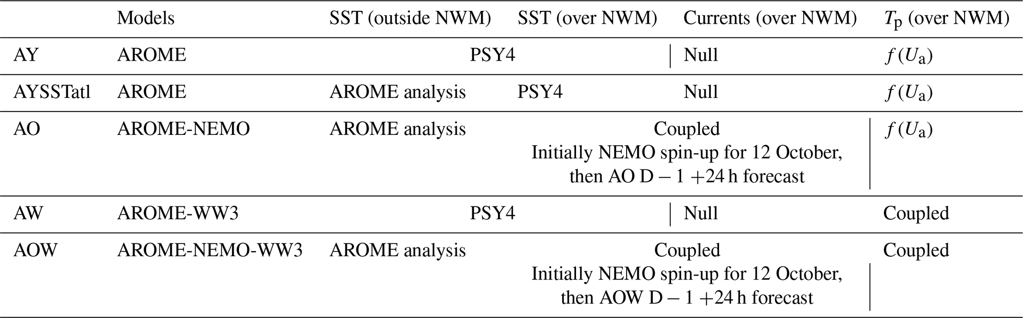
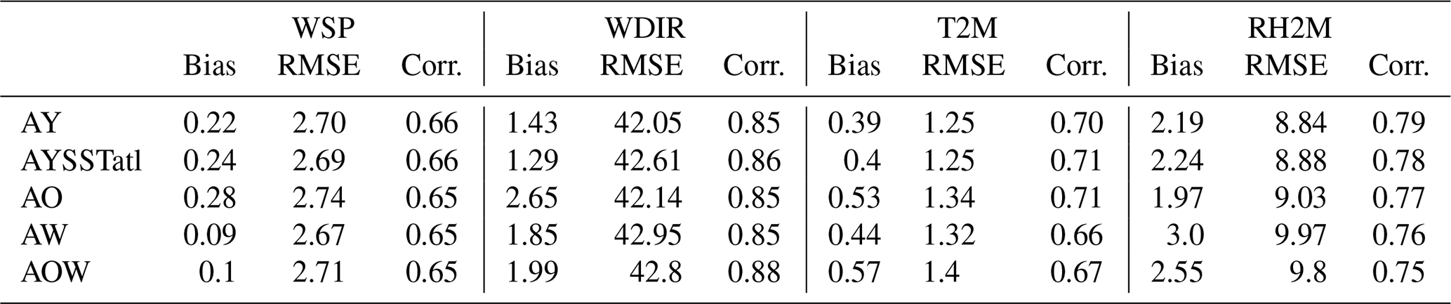
Table 3Scores against observations from moored buoys and surface weather stations for the 10 m wind speed (WSP, m s−1), the 10 m wind direction (WDIR, ∘), the air temperature at 2 m (T2M ∘C) and the relative humidity at 2 m (RH2M, %).
Two atmosphere-only experiments with AROME-France are also examined using the same atmospheric boundary and initial conditions as AOW but different SSTs. In the AY experiment, the SST initial field is taken from the PSY4 daily analyses for the whole marine domain of AROME-France, whereas in AYSSTatl, the SST forcing comes from the PSY4 analyses only on the NWM domain and from the AROME-France analyses elsewhere. Both AY and AYSSTalt use WASP as turbulent flux parameterization with the peak period estimated as a function of the surface wind, a constant SST field during the forecast and null current. Figure 3b shows the differences in SST between the AY and AYSSTatl simulations. The PSY4 SST from an ocean model at 112∘ resolution enables us to represent finer structures in the Atlantic Ocean (Fig. 3) compared to the AROME analysis, which only represents an average structure of the SST field. Differences in the Atlantic Ocean can be as high as 2 ∘C (3 ∘C locally). This simulation is in fact an intermediate simulation justified by the fact that the coupling with NEMO-NWMED72 leads to changes in SST only in the Mediterranean Sea. The comparison between AY and AYSSTatl thus allows for an assessment of the impact of the Atlantic Ocean surface temperature on the HPE forecast.
A summary of the sea surface conditions for each experiment is given in Table 2. The simulations AY and AW have already been used and validated in Sauvage et al. (2020) and serve here as references to evaluate the coupling impact.
Note that the insertion of ocean coupling here induces not only a prognostic evolution of the sea surface, but also modifications of the initial SST conditions seen by AROME-France over the NWM domain (Fig. 3c). These differences are induced by both the spin-up strategy and the restart mode of NEMO for each forecast run. Indeed, the spin-up (without assimilation) makes NEMO-NWMED72 slowly diverging from PSY4 but also allows it to produce its own fine-scale structures permitted by its resolution (172∘) and in response to the AROME-France high-resolution atmospheric forcing, whereas directly using the PSY4 3D fields would have let the ocean model adjustment affect the short-range forecast. The choice to restart NEMO for coupled forecasts from the spin-up first and then from a previous forecast was also made to be close to the cycling done in an operational context, i.e., using a previous forecast as initial conditions for the surface scheme (and as a background for the AROME 3D-Var data assimilation scheme, not done here). This way, the ocean model is initialized with adjusted, fine-scale, and instantaneous fields, which are representative of ocean conditions in the Mediterranean Sea before the event, while larger-scale daily-mean SST conditions are applied in fact in AY, AYSSTatl and AW with the PSY4 SST analyses.
Thus, regarding the study of Sauvage et al. (2020), the tri-coupling presented here adds new sea surface conditions, with the interactive evolution of the SST and of the currents simulated by NEMO at a kilometric resolution taken into account in the turbulent fluxes during the HPE forecast. This permits us (1) to verify the robustness of the results obtained on wave coupling impact, when an interactive ocean is included, and (2) to investigate and compare the coupling contributions to HPE forecast.
In order to quantify the impacts of coupling, a sensitivity analysis is conducted by finely analyzing the differences obtained. In particular, the contribution of the tri-coupled system (ocean–atmosphere–wave) will be compared to the impacts of the bi-coupled simulations (i.e., ocean–atmosphere and wave–atmosphere). The method thus consists in comparing the simulations two by two by estimating the impacts of the coupling (interactive evolution and changes in the initial conditions brought by coupling) on the dynamics (wind) and the low-level environment (temperature, humidity), the turbulent surface fluxes (momentum flux (or wind stress), sensible heat flux H and latent heat flux LE), evaporation and precipitation. When available, observations of the air–sea interface are also used to qualify the different simulations. The impacts of tri-coupling on the representation of the surface ocean layer and the sea state (Hs and Tp) are also examined.
4.1 Atmosphere–wave coupling
The analysis of the atmosphere–wave coupling is described in detail in Sauvage et al. (2020) with comparison of AW (AWC in Sauvage et al., 2020) to AY. Here are some highlights of the main conclusions.
The main result is a significant increase in the wind stress found along the French Riviera where the low-level wind is the strongest, as taking into account the sea state with the generation of a wind sea leads to an increase in surface roughness. The increase in stress in this region represents +10 % during Phase I (between 13 October 03:00 and 18:00 UTC) and +8.6 % during Phase II (between 13 October 19:00 UTC and 14 October 03:00 UTC) when compared to AY. The wave coupling has the effect of significantly reducing the wind speed along the French Riviera, up to 3 m s−1 and by 7 % in average with notably a decrease in bias at the Azur buoy. This is reflected in the overall wind speed bias in Table 3 presenting the bias, RMSE (root mean square error) and correlation coefficient calculated for each experiment with respect to weather surface stations. A spatial shift of about 15 km eastward of the convergence line and of heavy precipitation at sea is found, linked to the slowdown of the easterly wind upstream (along the French Riviera). In AW, a decrease in latent and sensible heat fluxes was noticed compared to AY. However, this decrease was only ∼2 % on the total turbulent heat flux, despite a priori favorable conditions for a larger response (i.e., strong winds, a large air–sea thermal gradient, and a young sea). Wave coupling also leads to significant differences in the Gulf of Lion, downstream of the convective system over the sea, related to internal modifications of the convective system. Finally, the convective system over the Hérault area appears not sensitive to wave coupling (or forcing). This can be explained by the fact that orographic uplift is the triggering factor of this system.
Adding the coupling with waves to an atmosphere–ocean coupled configuration can impact the heat extraction from the ocean in several manners (e.g., Renault et al., 2012; Varlas et al., 2020). First, taking into account waves can increase the surface roughness, leading to larger wind stress and weaker surface wind. This decrease in the wind can directly decrease the heat fluxes (see Eq. 5). Then, the increase in the surface roughness can result in larger transfer coefficients for heat (Eq. 8) that can lead to slightly larger heat fluxes. Finally, even though the ocean and wave models are not directly coupled in the present study, stronger wind stress can result in more mixing and cooling in the oceanic surface layer and thus colder SSTs. These colder SSTs can dampen the turbulent heat fluxes directly and also increase the atmospheric stability at a low level, further decreasing the surface wind and eventually the turbulent heat fluxes. In the present case, coupling with waves has almost no impact on SST (differences of less than 0.2 ∘C, not shown). The impact of the z0 increase on the heat transfer coefficients is also negligible (not shown). Conversely, the decrease in the simulated wind between AO and AOW is comparable to what was obtained between AY and AW and significant during Phases I and II, with differences of more than 1 m s−1 over a large area along the French Riviera (Figs. 4c and 2a for the location). As a result, latent and sensible heat fluxes are reduced in AOW by 3 % over Phases I and II (Figs. 5b and 6c, d), i.e., a slightly larger decrease than in AW/AY because of the nonlinear response of the heat fluxes to more unstable conditions in AOW/AO, and are mainly due to the slowdown of the wind. This result is in contrast with what was obtained in other case studies (e.g., Varlas et al., 2020), probably because the surface wind and the mixing in the oceanic mixed layer were much stronger than here.
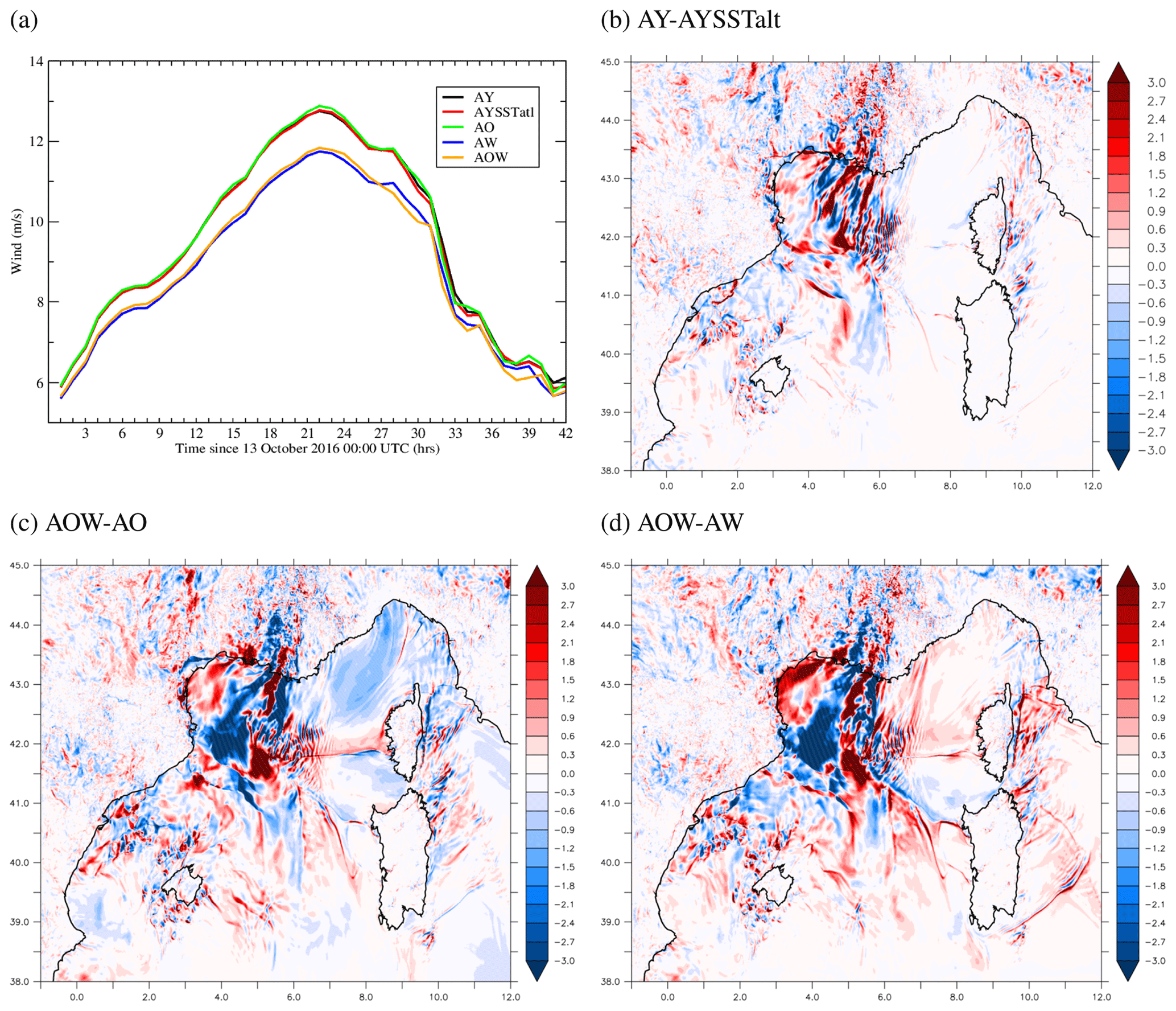
Figure 4(a) Time series of the surface wind (m s−1) forecasts on average over the Azur area and differences in surface wind at 00:00 UTC on 14 October between (b) AY and AYSSTatl, (c) AOW and AO and (d) AOW and AW (forecast basis: 13 October 00:00 UTC).
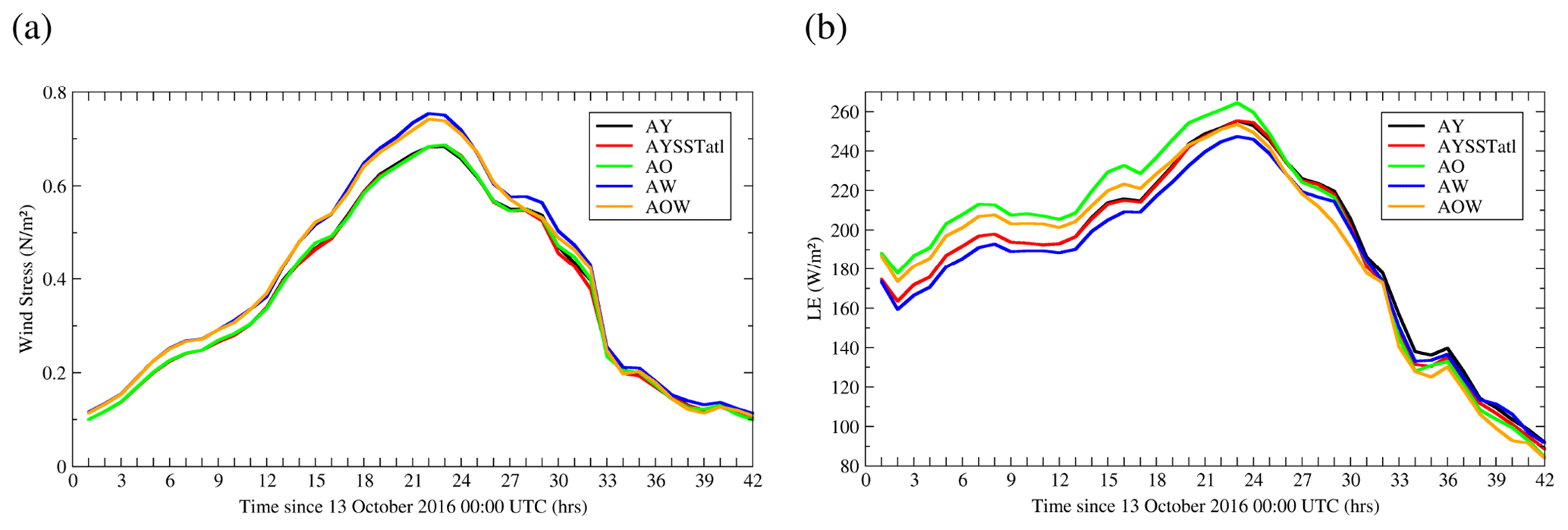
Figure 5Time series of (a) wind stress (N m−2) and (b) latent heat flux (LE, W m−2) on average over the Azur area for forecasts starting at 00:00 UTC on 13 October.
Figure 6LE differences (W m−2) (a, c) at 14:00 UTC on 13 October and (b, d) at 00:00 UTC on 14 October between AOW and AW experiments (a, b) and between AOW and AO experiments (c, d).
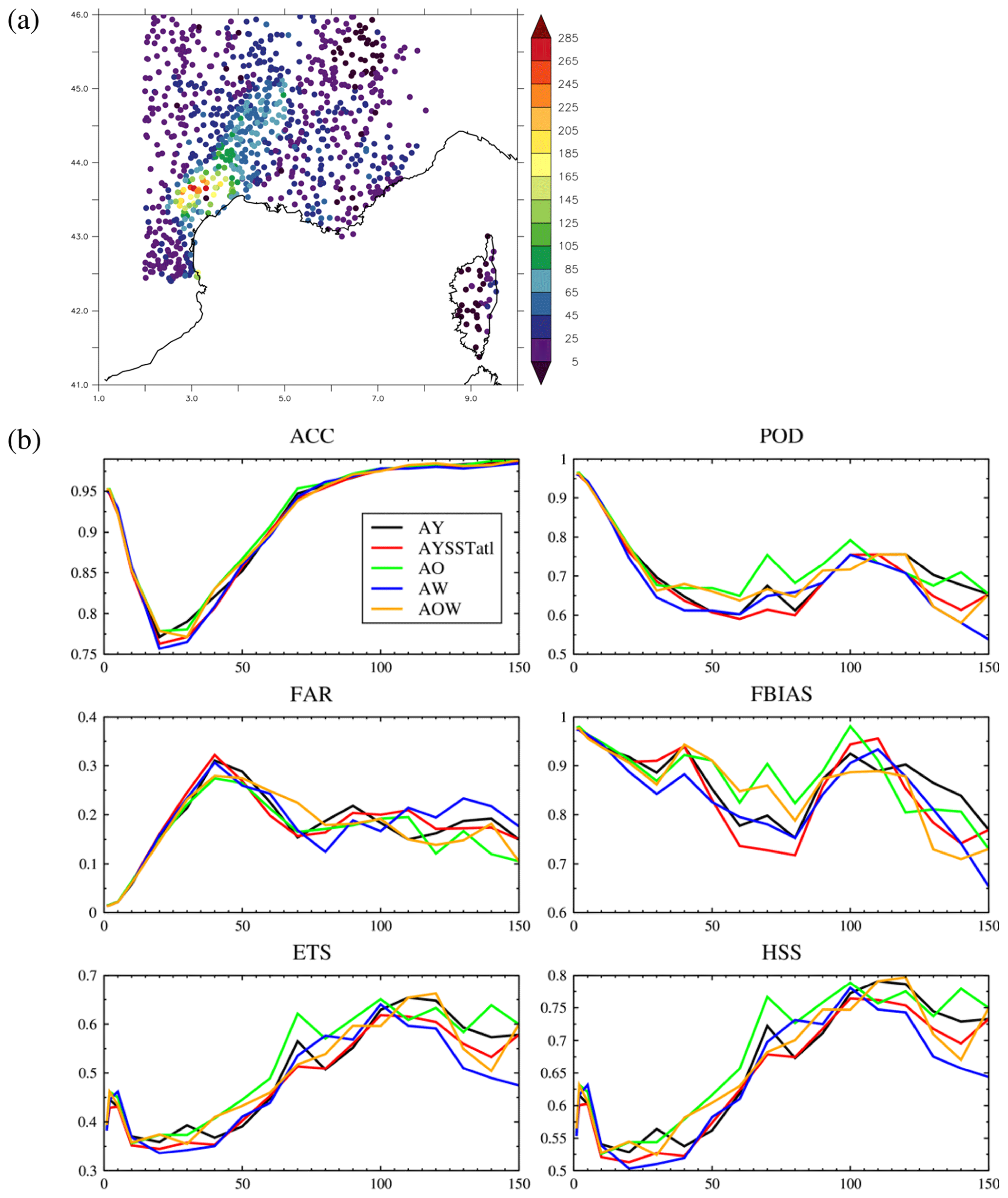
Figure 7(a) Locations and measurements of 24 h cumulative precipitation (mm) at 00:00 UTC on 14 October of the Météo-France rain gauges over the southeastern quarter of France. (b) Forecast skill scores against rain-gauge observations calculated for cumulative rainfall in 24 h at 00:00 UTC on 14 October. The x axis indicates the rainfall threshold considered, in millimeters.
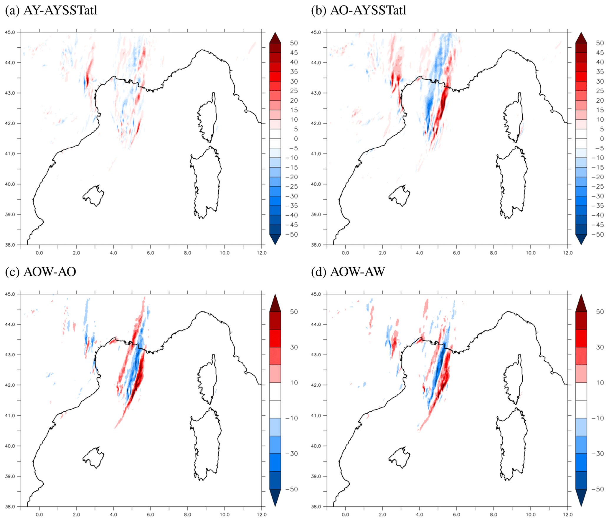
Figure 8Differences in 6 h cumulative precipitation (mm) at 00:00 UTC on 14 October (a) between AOW and AO and (b) between AOW and AW.
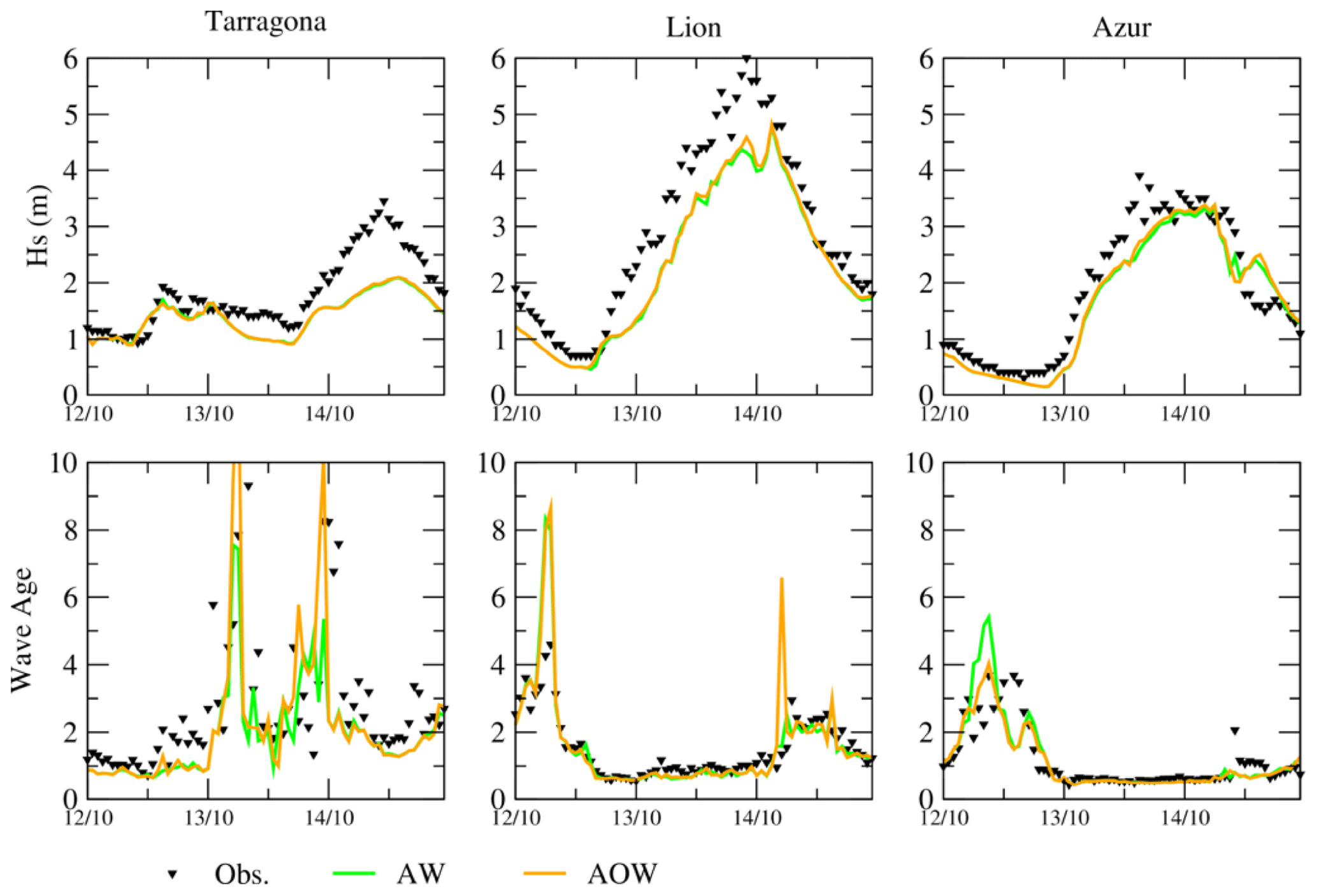
Figure 9Time series of simulated significant wave height Hs and wave age at the three moored buoys Tarragona, Lion and Azur at 00:00 UTC on 12 October to 00:00 UTC on 15 October, using successive forecasts of each experiment including WW3 (+1–+24 h forecast ranges each day).
Figure 7a presents different probability scores according to 24 h precipitation accumulation (between 13 October 00:00 UTC and 14 October 00:00 UTC) thresholds (Ducrocq et al., 2002): ACC (accuracy), POD (probability of detection), FAR (probability of false alarm), FBIAS (frequency bias), ETS (equitable threat score) and HSS (Heidke skill score) are calculated by comparison to rain-gauge observations shown in Fig. 7b. The FAR score is better when it is close to 0; for the others, a score of 1 is relative to a perfect prediction. Precipitation scores between AOW and AO are close for cumulative thresholds between 0 and 50 mm. More variability appears for higher thresholds, but overall AO performs better than AOW. The addition of wave coupling slightly reduces the intensity of precipitation over the Hérault area on average and with a maximum 24 h amount in AOW of 264 mm compared to AO with 306 mm (Table 4). Except for this punctual decrease in the maximum, the heavy rainfall event over Hérault in AOW is very similar to the one in AO (chronology, area and mean amount, Fig. 8c; see Fig. 2c for the location), and so there is no degradation due to the inclusion of the wave coupling from a NWP and/or early warning perspective.
For precipitation related to the MCS over the sea, the wave coupling induces larger mean values when comparing AOW with AO (Table 4). Figure 8c shows the differences in the 6 h accumulation of precipitation at 00:00 UTC on 14 October between AOW and AO, i.e., during Phase II. A slight eastward shift of a few kilometers in the location of the precipitation is seen. Since the near-surface wind in AOW decreases (compared to AO) in the same way as in AW (compared to AY), this shift in the location of the convergence and heavy precipitation at sea is likely due to the same process, i.e., a higher roughness in the Ligurian Sea and a slowdown of the easterly low-level atmospheric flow.
Table 4Simulated maximum and mean values of rainfall amounts (mm) in 24 h at 00:00 UTC on 14 October over the Hérault zone and the offshore zone around MCSs for the different experiments (forecast starting at 00:00 UTC on 13 October).
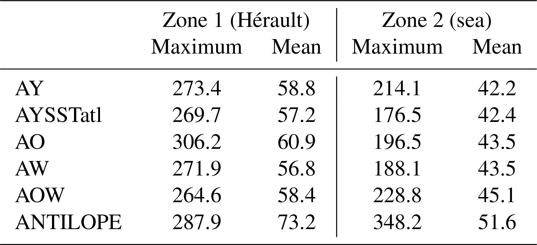
Table 5Scores against wave observations from moored buoys and satellites for Hs (m) and Tp (s).
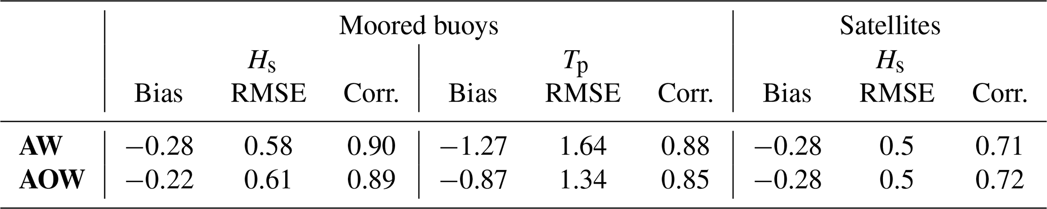
Comparisons with sea state recorded by moored buoys are additionally used to assess the quality of the wave forecast in AOW and AW simulations. The scores calculated for the sea state parameters are summarized in Table 5. Few differences in Hs and Tp scores are obtained when comparing AOW to AW, with a reduction in bias for moored buoys, a reduction in RMSE for Tp, and a slight decrease in correlation in AOW. The evolution of the sea state during the event is described for three moored buoys – Tarragona, Lion and Azur – in Fig. 9. The Hs time series simulated by AOW and AW are very close. Nevertheless, we observe a trend of increasing values of Hs and Tp in AOW, with for example for Hs+20–40 cm locally in the Gulf of Lion and along the French Riviera that represents an increase on the order of 1 %–2 % on average in these areas.
The differences in Hs are larger around 00:00 UTC on 14 October, particularly under the convective system. A difference dipole of ±1 m corresponds in fact to a shift of the maximum Hs values due to the different positioning of the MCS at sea at that time between AOW and AW. The time series of the wave age during this period show small changes between the simulations (Fig. 9), and we conclude that the characteristics of the sea state forecast remain the same in AW and AOW, with a wind sea (corresponding to wave age <1) well represented at Lion and Azur.
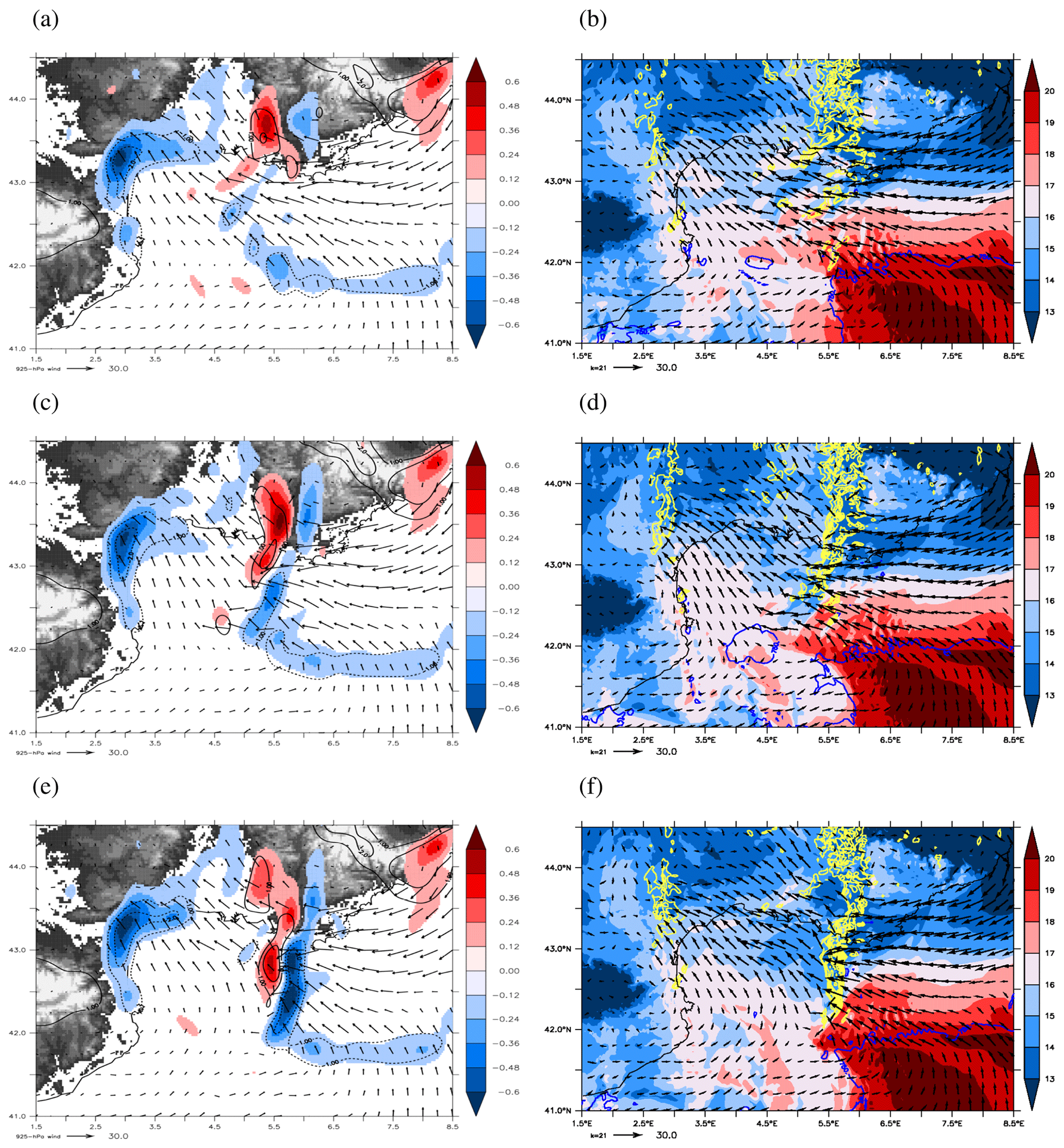
Figure 10(a, c, e) Wind divergence (10−3s−1) at 950 hPa, vertical velocity (Pa s−1, black contours) at 950 hPa and surface wind at 925 hPa (m s−1, arrows). (b, d, f) at 925 hPa (∘C), CAPE (>750 J kg−1, dark blue line), and surface wind at 925 hPa (m s−1, arrows) and reflectivities at 2000 m (dBz, yellow line) at 00:00 UTC on 14 October for (a, b) AYSSTatl, (c, d) AO and (e, f) AOW.
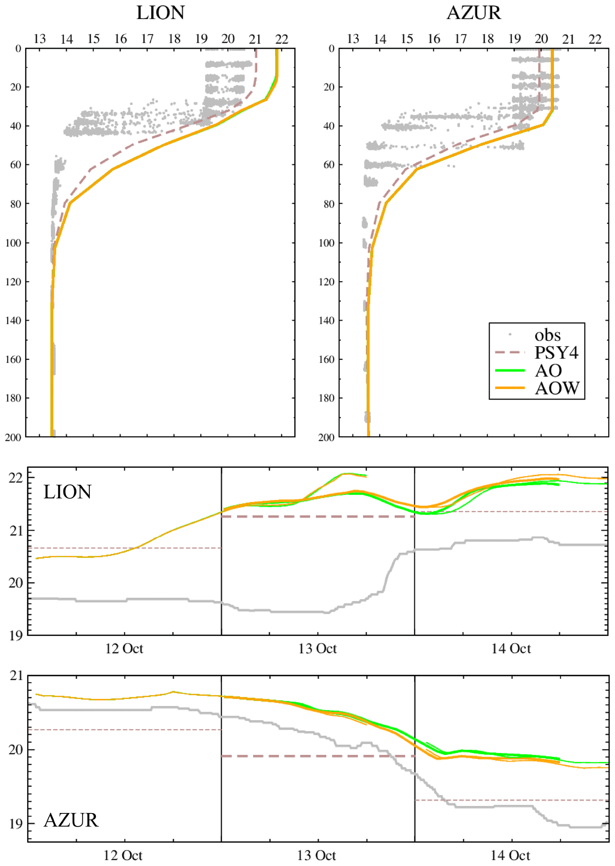
Figure 11Upper panels: ocean temperature profiles (∘C) observed by the chains of thermistors at the Lion (left) and Azur (right) buoys between 12 and 14 October (grey dots) and simulated by AO and AOW on average for the day of 13 October. Temperature profiles in the PSY4 operational system analysis of 13 October are shown in dashed lines. Lower panels: 6 m depth ocean temperature time series (∘C) observed at Lion and Azur and simulated by AO and AOW (successive forecasts). The dashed lines correspond to the values in PSY4.
4.2 Atmosphere–ocean coupling
As stated in Sect. 3.2, introducing the ocean coupling consists of an interactive ocean model and a change in the initial SST condition. Figure 3c represents the difference in initial SST in the Mediterranean at 00:00 UTC on 13 October between AOW and AW (i.e., the PSY4 analysis). The initial SST is warmer in AOW, especially in the Gulf of Lion, along the French Riviera and in the Tyrrhenian Sea (up to 1.5 ∘C). At 00:00 UTC on 14 October, after 24 h of forecast, the SST in AOW cooled down (Fig. 3d), especially in the Gulf of Lion and along the French Riviera where winds and heat fluxes are strongest (Fig. 2a, b). In these areas, larger evaporation and latent heat flux are found in AOW compared to AW (+7 % in the Azur zone during Phase I, Figs. 5b and 6a, b) due to a warmer SST at the beginning of the event. The sensible heat flux in AOW is also increased by 11 % during Phases I and II compared to AW (not shown). This allows more heat and moisture extraction from the ocean mixed layer to the atmospheric low levels and therefore more favorable low-level conditions for convective systems. In the last part of the event, coupling with the ocean results in slightly colder SSTs in AOW than in AW and slightly lower enthalpy fluxes. Ocean coupling appears to have a small impact on wind stress and surface wind speed: both simulated parameters in AOW are on average identical to those of AW along the French Riviera and in the Gulf of Lion, with differences of less than 0.3 m s−1 (Figs. 5a and 4a, d). The largest differences are found in the Gulf of Lion in the form of dipoles that are not homogeneous in time. These patches of differences are mainly due to modifications in the evolution of convective cells and small displacements of the MCS over the sea in the different simulations, with consequences for the low-level flow downstream. The same results are observed when comparing heat fluxes and surface dynamics between AO and AYSSTatl. In view of these results, it confirms that ocean coupling including change in the initial SST and taking into account the interactive SST and surface currents in the wind stress computation has a very low impact on the near-surface wind for such a strong wind regime largely controlled by the synoptic circulation.
For temperature (T2M) and relative humidity (RH2M) at 2 m, small differences are obtained on average between the simulations. T2M varies from 1 % to 3 % on average with a tendency to increase for T2M when the atmosphere is coupled with the ocean (and/or waves). For RH2M, coupling with the ocean has a small impact (<1 %) that in fact corresponds to an increase in the specific humidity at 2 m (not shown) associated with the low-level warming. Although these differences are, on average, not significant, larger differences can be observed at any given time along the French Riviera and under the convective system in the Gulf of Lion (not shown).
Coupling with the ocean results in more intense precipitation for the system on the Hérault with a larger mean rainfall amount (Table 4 and Fig. 8b) and a maximum 24 h rainfall amount at 00:00 UTC on 14 October of 306 mm in AO versus 269 mm in AYSSTatl. This is due to a slightly moister and warmer air mass at low levels over the Gulf of Lion leading to a more intense convection. At sea, an increase in the maximum 24 h rainfall amount is obtained in AOW (228 mm) compared to AW (188 mm) (and in AO (196 mm) compared to AYSSTatl – 176 mm), but the mean value remains close. Overall, rainfall scores are better in AO (and AOW) compared to AYSSTatl (and AW) (Fig. 7b). The differences in the 6 h accumulation of precipitation at 00:00 UTC on 14 October between AOW and AW appear quite similar to those between AOW and AO, especially for the offshore system (Fig. 8c, d), because of a slight eastward shift of a few kilometers in the location of the precipitation. The effect of ocean coupling on precipitation, however, involves a different mechanism than wave coupling. Indeed, the addition of the ocean coupling with a warmer initial SST allows for a larger input of heat and moisture due to higher evaporation and heat fluxes during the initiation phase. This leads to an intensification of the system at sea with formation of a cold pool, which reinforces and tends to push eastwards the convergence during the mature phase (Fig. 10).
The strong sensitivity of the convergence at sea to changes in initial SST and to the oceanic feedback was already highlighted by Rainaud et al. (2017) with the AROME-NEMO coupling for another Mediterranean HPE. The present study permits us to identify more clearly the large impact of ocean initialization and coupling on heat and water supply, which controls the intensity of convection which itself modifies the MCS motion and location through internal mechanisms acting for this case to a convergence reinforcement.
Concerning ocean forecasts, AOW and AO simulations show very similar results, with a positive bias in temperature (0.57 ∘C) and almost null in salinity (−0.02 psu) when compared to moored and drifting buoy observations between 12 October 00:00 UTC and 15 October 00:00 UTC (using the +1 to +24 h forecast ranges for each day). The thermohaline characteristics of intermediate and deep waters are very well represented. If we consider only the upper-ocean layer (0–100 m), the biases are larger (about −1 ∘C and −0.05 psu, respectively). The most important errors are located between about 15 and 60 m, with biases up to 6 ∘C and −0.9 psu. These large differences actually reflect an issue in the representation of the thermocline and halocline, which are deeper but also smoother in the model. Figure 11, comparing the simulated temperature profiles at the Lion and Azur buoys, shows indeed that the mixed layer is thicker and especially that the thermocline is less marked than observed. The same defect of a less marked thermocline (halocline) is found in the analyses of the ocean operational system PSY4 when compared to the same observations, which shows that the biases of AOW and AO are in fact largely inherited from the ocean initial state used. Also, Fig. 11 shows the cooling at the Azur buoy under the strong easterly wind observed all along the event (−0.75 ∘C in 24 h and −1.4 ∘C in 42 h observed since 00:00 UTC on 13 October). This ocean response appears quite large considering other HPE studies (e.g., Lebeaupin Brossier et al., 2009, 2014; Rainaud et al., 2017) and is comparable to other high-wind or medicane events (e.g., Renault et al., 2012; Bouin and Lebeaupin Brossier, 2020a). Even though it is significant, it appears to be underestimated by the model (−0.6 ∘C in 24 h and −0.85 ∘C in 42 h simulated by AOW). Overall, this default in representing the cooling can be explained by the initial ocean state with a too smooth thermocline that limits the mixed-layer cooling by entrainment, by physical parameters and/or schemes in NEMO and by the absence of ocean–wave coupling.
The comparison of the AOW tri-coupled experiment with the AY atmosphere-only experiment highlights that the combined effect of couplings is an increase in wind stress and enthalpy flux during the initiation and mature phases in the Azur area (Figs. 5 and 6). Here and all along the two phases, the low-level wind is reduced upstream of the offshore MCS (Fig. 4). As a consequence of larger heat and moisture supplies, both convective systems over Hérault and over the sea are more intense and lead to larger precipitation amount forecast (Fig. 8 and Table 4). In AOW, the more intense MCS over the sea tends to reinforce the convergence (Fig. 10), which is displaced by nearly 100 km eastwards compared to AY.
In fact, the analysis of the coupled simulations AW, AOW, and AO shows the high sensitivity of the location of the heavy precipitating MCS at sea, as an eastward shift of several kilometers of the system is seen with any coupling (Fig. 8). However, the mechanisms identified for this response appear different between wave coupling and ocean coupling. On the one hand, the dominant process with wave coupling is the slowing down of the easterly flow due to more roughness that shifts the location of the convergence line, whatever the surface heat flux values are (related to SST or low-level wind variations). On the other hand, ocean coupling and its initialization strongly control the heat and moisture supply that indirectly impacts the convergence through internal modifications of the convective system (more intense if a higher SST is used during the initiation and mature stages). Thus, these results prove the importance and complementarity of both couplings to well represent the complex interactions of the ocean upper and surface layers with the marine atmospheric boundary layer, in particular for such severe weather conditions with large exchanges.
The clear splitting between the two coupling impacts on the atmospheric event here has been done thanks to bi-coupled experiments and confirmed in AOW, where there is no direct interaction between ocean and waves. However, it has been shown that surface waves enhanced vertical mixing in the ocean surface layer. In the case of tropical cyclones, Aijaz et al. (2017) for example showed that wave-induced mixing caused significant cooling and a deepening of the mixing layer, which can then impact the intensity of the cyclone. Staneva et al. (2016) and Wu et al. (2019) also showed with sensitivity studies in the North Sea and Baltic Sea that taking into account the effect of waves on the ocean improved surface temperature, ocean surface circulation and sea level height. So, it would be interesting to conduct other experiments by adding the interactive coupling between ocean and waves, as it would likely modify the turbulence and the exchanges at the air–sea interface. The use of the SURFEX-OASIS coupling interface enables us to quickly consider the insertion of the full coupling between NEMO and WW3, as recently developed by Couvelard et al. (2020) with updates in the physics of NEMO (v3.6) and validated through a global coupled modeling study. As mentioned in Sect. 4.2, the SST initial field is of great importance for short-term forecast of extreme events involving large air–sea fluxes (e.g., Lebeaupin Brossier et al., 2009; Rainaud et al., 2017). The spin-up strategy used to start NEMO in the AO- and AOW-coupled simulations induced large discrepancies when compared to the PSY4 daily analysis (Fig. 3) as in AROME-only simulations (AY or AYSSTatl). On the other hand, the use of the PSY4 SST daily analysis to start the forecast means that initial conditions (i.e., at 00:00 UTC) are actually a 24 h average of the SST, including changes in SST due to the studied event. To better illustrate this initialization issue, the comparison of the 6 m-depth temperature at Azur in Fig. 11 shows that starting with the PSY4 analysis on 13 October leads to a significant initial cold bias compared to observations (−0.5 ∘C, similarly for SST) as PSY4 already accounts for the cooling during that day. For atmosphere-only or atmosphere–wave forecasts, the SST bias reduces with time, while this error would have persisted then if it had been used to initiate NEMO in the AO- and AOW-coupled experiments. So, for coupled forecast of HPEs or other severe weather events happening over a short period of time (<24 h), an ocean initial state corresponding to an hourly average for example or to an instantaneous state is preferable to avoid this potential bias prolongation.
Moreover, we investigated the influence of the Atlantic Ocean surface conditions on the AROME forecast by comparing AY and AYSSTatl. As expected, the Atlantic Ocean SST differences between AY and AYSSTatl have a small impact on low-level conditions in the Mediterranean area, as the latent heat flux and the wind stress are on average identical, especially along the French Riviera (Fig. 5). The scores in Table 3 confirm that AY and AYSSTatl are similar for precipitation forecast. The scores of AY and AYSSTatl are also close for thresholds between 0 and 50 mm. We note more variations for larger rainfall amounts, with overall a slight improvement in AY (when SST from PSY4 is used in the Atlantic rather than the AROME analysis). Thus, the difference in SST over the Atlantic Ocean has a very small impact. Indeed, for this event driven mainly by eastern and southern flows that supply MCS in heat and moisture extracted from the Mediterranean Sea, the change in SST in the Atlantic has a small influence on these low-level flows. However, the change in SST may have had an impact on the position of the cold front and disturbed the convergence affecting, in particular, the formation and movement of the MCS at sea, which may explain the slightly larger differences found in the Gulf of Lion.
Regarding the ocean surface current coupling, recent studies highlighted the importance of the representation of the current–wind interactions and the atmosphere feedback for the ocean mesoscale structures (e.g., Seo et al., 2016; Seo, 2017; Renault et al., 2016; Jullien et al., 2020). Renault et al. (2017, 2019) showed a damping of the eddy kinetic energy due to the current feedback modulation of the energy transfer between the ocean and the atmosphere leading to more realistic simulations. These current–wind interactions need to be further investigated in our coupled system with the insertion of the current terms in the AROME turbulence scheme. However, in this particular HPE case, as the near-surface wind speed is largely superior (>20 m s−1) to the surface current velocity (<1 m s−1), we hypothesize that the feedback of the surface current on the atmosphere might be small (as in Bouin and Lebeaupin Brossier, 2020b, for instance).
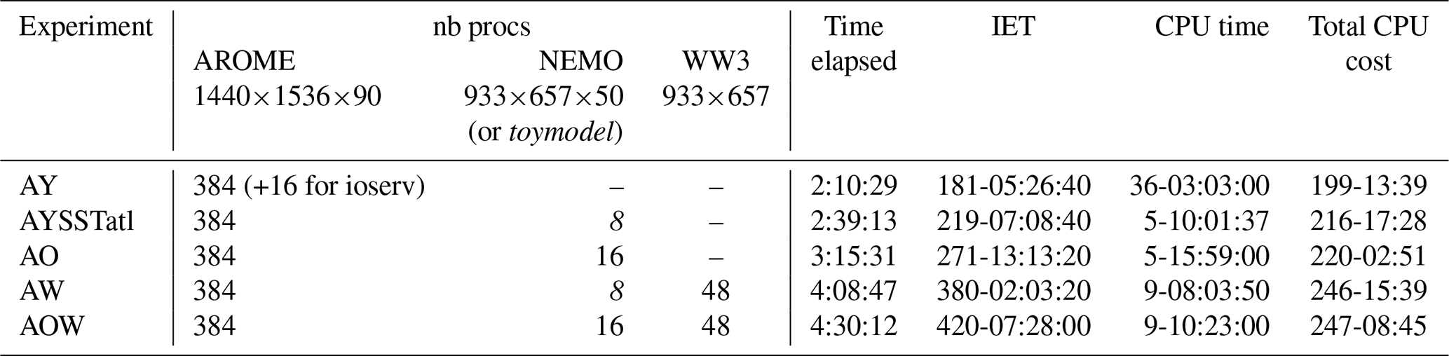
The numerical performances of the various simulations are finally briefly summarized here and described in more detail in Appendix B. Compared to AYSSTatl, the ocean coupling in AO increases the total CPU cost by 1.6 % and, thus, the ocean coupling can be considered very light in terms of computing cost. The wave coupling in AW increases the total CPU time by 13.8 % with respect to AYSSTatl. The elapsed times are also increased with coupling, by 22 % for ocean and 57 % for wave. Considering the delivery constraint in an operational forecasting system, this represents a significant increase. However, it must be said here that no specific efforts have been made in input/output (I/O) management for the various models and to balance the various computation times, although possible using a higher number of processes notably for WW3, and to optimize the calculation time on the Météo-France High Performance Computing system (HPC), and thus improvement in this matter needs to be done, in particular concerning WW3 compilation options. Finally, AOW shows increases in computation cost and time consistent with the addition of the two couplings.
This study presents the ocean–atmosphere–wave coupled system, developed using the NWP model AROME, the NEMO ocean circulation model and the wave model WW3, all at a kilometric resolution. This system is designed to better understand and represent the exchanges at the air–sea interface and to evaluate the impact on the weather forecast using a case study corresponding to a Mediterranean HPE that occurred in mid-October 2016. In order to quantify the contributions of the different couplings, a set of bi-coupled and tri-coupled simulations was carried out. Sensitivity analysis highlighted the importance of coupling with waves on the dynamics of the lower levels of the atmosphere. Indeed, the slowdown of the near-surface wind along the French Riviera occurring in AW is preserved in the same proportions in the AOW tri-coupled experiment. Compared to these results, the coupling with an interactive ocean appears to have a small impact on the momentum flux and on the surface wind. Nevertheless, the coupling with the ocean plays an important role in air–sea heat exchanges. Due to the ocean initialization with better and more timely solved and instantaneous fields, the warmer ocean in AO increases heat and moisture extraction during the initiation and mature stages of the event and therefore changes the development of the convective systems. This also affects the convergence line at sea with the establishment of a better-organized system. Regarding the heavy precipitation over the Hérault region, we observe a weak variability through the different simulations, which can be explained by its triggering mechanism that is mainly controlled by orographic uplifting. The offshore system shows a greater sensitivity to coupling with, in particular, displacements of the convergence line inducing differences in intensity and location of the heavy precipitation.
The validation of the ocean compartment with in situ observations showed a good representation of the near-surface ocean layer and showed no significant impact due to wave coupling in AOW. The validation of the wave compartment, when comparing AW and AOW, also showed little differences despite a decrease in the bias (and RMSE) for Tp in the AOW simulation. These results permit us to be confident in the numerical and scientific benefits of coupling ocean and wave forecasts to the atmosphere even for short-range forecast and in the feasibility of integrated forecasts.
More generally, the current development of high-resolution coupled models allows us to resolve phenomena at a kilometric scale. The recent deployments of new airborne or spaceborne observing capabilities enable us to detect very fine structures at the sea surface (sharp SST fronts, filaments, strong contrasts of currents for instance) thanks to their signature on the surface roughness (e.g., Rascle et al., 2017; Wang et al., 2019). These surface sub-kilometric features of oceanic or meteorological origin are likely present as small-scale modulations of a larger-scale gradient of SST, surface current or wave field. Oceanic modeling is now able to accurately represent such structures and their time evolution, provided the resolution of the simulation is fine enough (e.g., Gula et al., 2014). SST fronts for instance can significantly impact the atmospheric conditions (Small et al., 2008), low-level flow (Redelsperger et al., 2019) and convergence (Meroni et al., 2020) independently of strong-impact weather events. The feasibility of using tri-coupled configurations like the one developed in the present study for a reasonable computing cost opens the way to a more explicit representation of the surface heterogeneities at sea, of their time evolution, and of their impact on the atmosphere for high-resolution deterministic operational NWP. If coupling allows more realism, the quality of coupled forecasts remains however still constrained by the resolution of computations, by the approximations in some physical process parameterizations and by the shortcomings of the observing systems initializing the different numerical models involved. So, to carefully separate a predictive value from the noise related to coupled forecast errors, further studies need also to be conducted to examine the propagation of uncertainties in a coupled system through ensemble coupled experiments, which are now within our reach, for a larger number of cases covering a larger range of weather situations.
Tables A1, A2, A3 and A4 specify the parts inserted into the various namelists for the AOW-coupled simulation. The reader can also refer to the user documentations of SURFEX, WaveWatchIII, NEMO and OASIS.
Table A1SURFEX namelist (EXSEG1.nam) parameters used for coupling (AOW experiment).
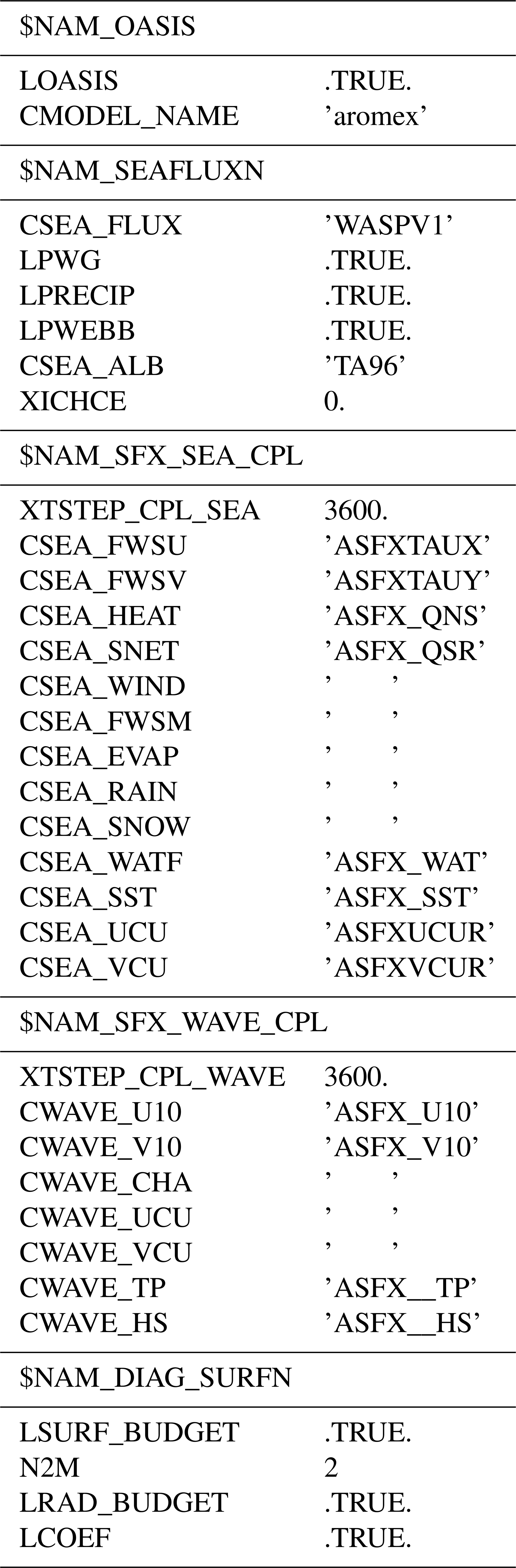
Table A2Part dedicated to coupling in the WaveWatch3 namelist (ww3_shel.inp) for the forecast starting on 13 October 2016 00:00 UTC (AOW experiment).
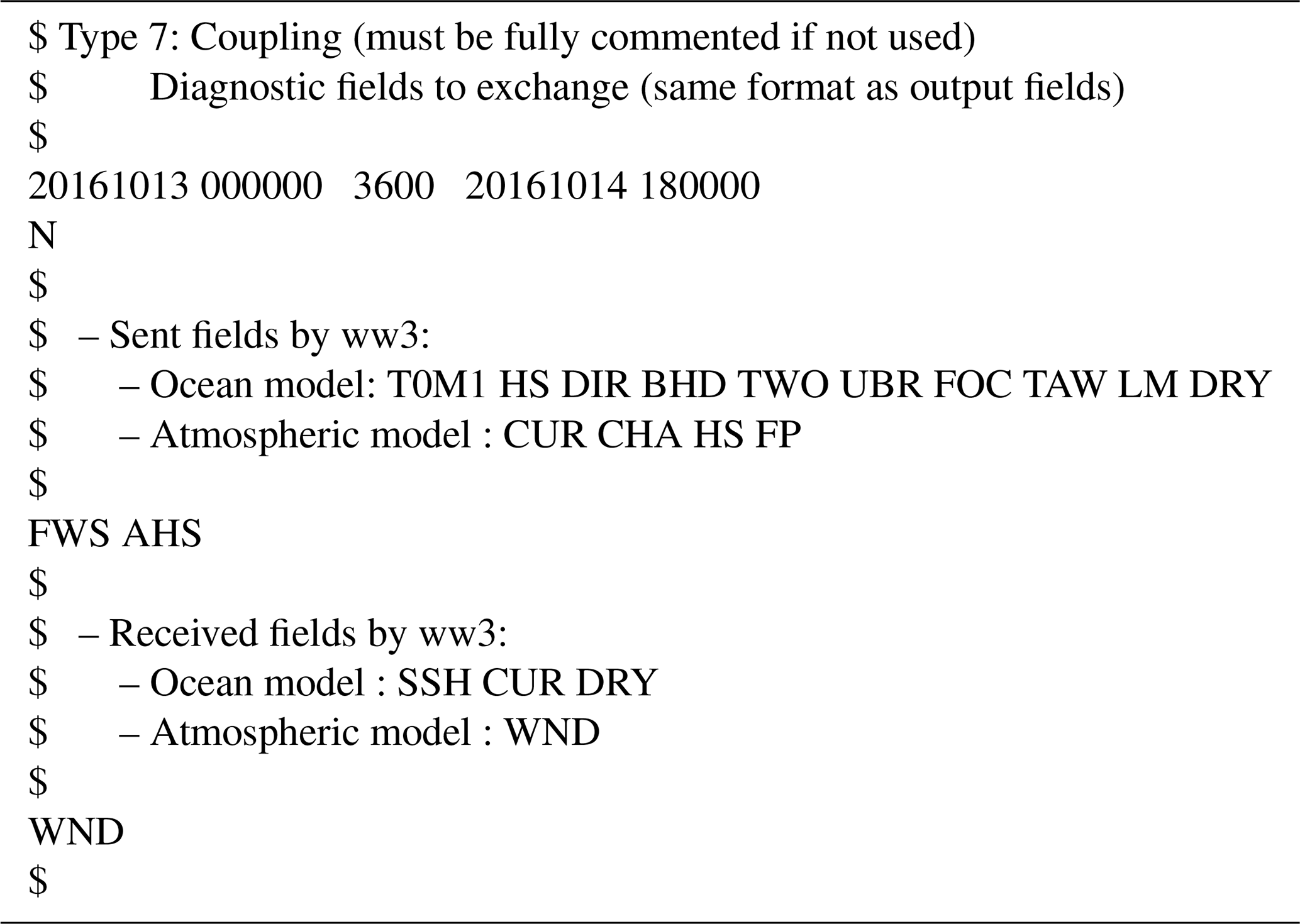
Table A3NEMO namelist (namelist_cfg) parameters used for coupling (AOW experiment).
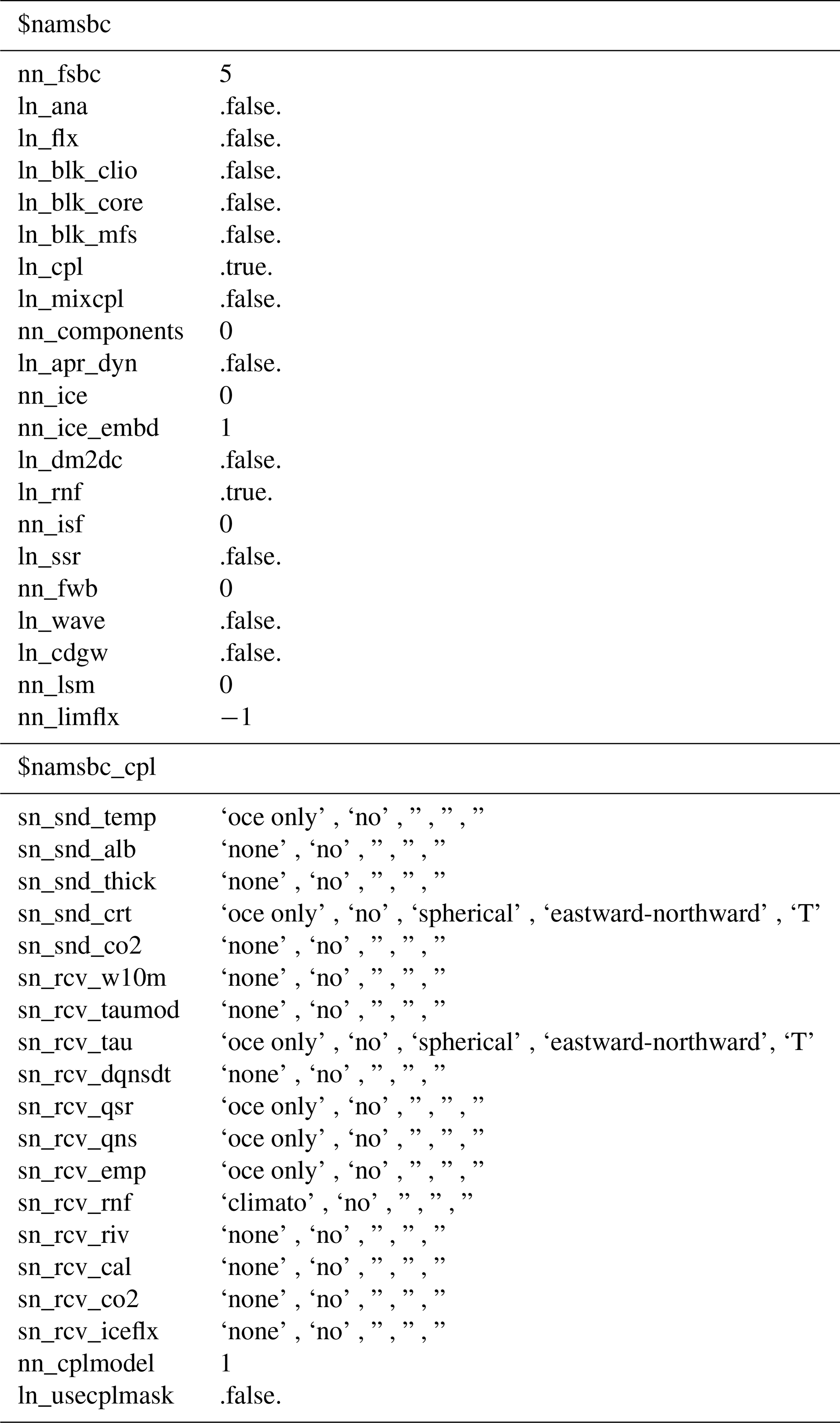
Table A4OASIS namelist (namcouple) details for the AOW experiment: torc or tww3 is the NWMED72 grid name, taro is the full AROME-France grid name, and tame is the AROME-France grid name masked (to land) outside the northwestern Mediterranean sea domain.
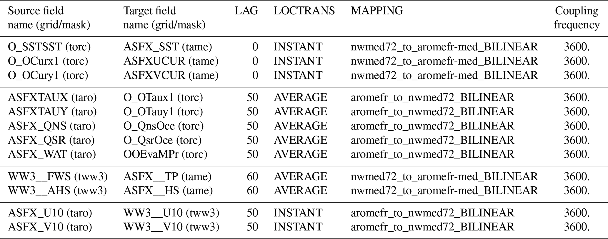
$NFIELDS is set to 12 and $RUNTIME to 151200, and the line for $NBMODEL is `3 aromex oceanx wwatch 99 99'
Table B1 describes the numerical performances of the simulations for 42 h range forecasts. First, it is important to note that only AY uses the AROME uncoupled binary and AROME I/O server, with a distribution of 8 processes by core (i.e., 48 cores of 8 processes for AROME and 2 cores of 8 processes for its I/O server). The AYSSTatl simulation is an atmosphere-only simulation but is related to a toy model through the SURFEX-OASIS interface in order to initiate SST from two various sources (AROME and PSY4 analyses) as imitating an ocean model. Also, the AROME I/O server is switched off in AYSSTatl (as for all simulations using OASIS) because the MPI (message-passing interface) link between OASIS and the AROME I/O server is not inserted yet. The choice was made to always keep the distribution of 8 processes by core, and thus the toy model allocates one core of 8 processes, while AROME keeps 48 cores of 8 processes (i.e., 384 processes in total). The comparison of AYSSTatl with AY shows an increase in the time elapsed (+22 %) and in the total central processing unit (CPU) cost (+8.5 %) and a large loss of efficiency (shown by the CPU time values) due to the fact that the toy model processes are “sluggish” all forecast long and also due to the cost of an undistributed I/O task.
Hereafter, the coupled forecasts are compared to AYSSTatl. The ocean coupling in AO increases the total CPU cost by 1.6 %, with only two cores of eight processes allocated for NEMO, and the time elapsed by 22 %. This latter increase is in fact related to the rebuild task that reassociates the NEMO output files of each process in a single file containing the whole NWMED72 domain. For future versions of the coupled system, this will be completely avoided with the use of the XIOS library (XML-IO-Server, Meurdesoif, 2013) to manage the NEMO outputs. The wave coupling in AW is done with six cores of eight processes for WW3 and one core to manage the SST field with a toy model. It increases the total CPU time by 13.8 % and the time elapsed by 57 % with respect to AYSSTatl. Finally, AOW shows both increases in elapsed time (and integrated elapsed time – IET) and in total a CPU cost consistent with the addition of the two couplings.
Table B1Computation scaling on Météo-France HPC for a 42 h-range forecast.
Although the operational AROME code cannot be obtained, the modified sources for cy41 are available on demand to the authors for the partners of the ACCORD consortium and will be included in the cycle 48 Météo-France official release. The source codes of the other components are available online.
-
WaveWatchIII was used in version 5.16, which is distributed under an open-source style license through a password-protected distribution site at https://polar.ncep.noaa.gov/waves/wavewatch/ (last access: 5 August 2021) (NOAA/NCEP, 2021a). Since version 6.07, WaveWatchIII is distributed using GitHub (https://github.com/NOAA-EMC/WW3, last access: 5 August 2021) (NOAA/NCEP, 2021b) without any username and password required to access the software package.
-
NEMO is available at https://www.nemo-ocean.eu/ (last access: 5 August 2021) (NEMO, 2021) after user registration on the NEMO website. The version used is NEMO_v3.6_STABLE for Mediterranean configurations (see https://sourcesup.renater.fr/wiki/morcemed/nemconfig, last access: 5 August 2021, Institut Pierre Simon Laplace, 2021 and Appendix).
-
OASIS3-MCT was used in version OASIS3-MCT_3.0. It can be downloaded at https://portal.enes.org/oasis (last access: 5 August 2021) (CERFACS, 2021). The public may copy, distribute, use, and prepare derivative works and publicly display OASIS3-MCT under the terms of the Lesser GNU General Public License (LGPL) as published by the Free Software Foundation, provided that this notice and any statement of authorship are reproduced in all copies.
-
The SURFEX open-source version (Open-SURFEX), including the interface with OASIS from v8_0, is available at http://www.umr-cnrm.fr/surfex/ (last access: 5 August 2021) (CNRM, 2021) using a CECILL-C Licence, a French equivalent of the L-GPL licence (https://www.umr-cnrm.fr/surfex/IMG/txt/licence_cecill_c_v1_en.txt (last access: 5 August 2021) (UMR-CNRM, 2021) but with the exception of the Gaussian grid projection, the LFI and FA I/O formats, and the dr HOOK tool. The sources for wave–atmosphere coupling within the SURFEX-OASIS interface and the WASP parameterization will be included in the next release (v9) of SURFEX but can be provided on demand by the authors for older SURFEX versions (back to v7_3).
Outputs from all simulations discussed here are available upon request to the authors.
The Antilope product can be made available for research purposes upon request (contact: olivier.laurantin@meteo.fr). The surface weather station data and the chains of thermistors on the Lion and Azur Météo-France moored buoys are available in the MISTRALS/HyMeX database (https://mistrals.sedoo.fr/, last access: 5 August 2021) (MISTRALS, 2021) after subscription. Oceanographic buoy data and the PSY4V3R1 daily analyses of Mercator Ocean International are available through the Copernicus Marine Environment Monitoring Service (CMEMS) portal (https://marine.copernicus.eu/, last access: 5 August 2021) (CMEMS, 2021) after user registration.
All the authors (CS, CLB, and MNB) contributed to the conceptualization and methodology of the study as well as drafting, reviewing and editing the article. MNB developed the WASP parameterization and managed its integration into the SURFEX code. The configuration NWMED72 of both the NEMO and WaveWatchIII models was developed and coupled to AROME by CS and CLB. Simulations were run by CS. CS, CLB and MNB carried out the validation and analysis of the results.
The authors declare that they have no conflict of interest.
Publisher's note: Copernicus Publications remains neutral with regard to jurisdictional claims in published maps and institutional affiliations.
This article is part of the special issue “Hydrological cycle in the Mediterranean (ACP/AMT/GMD/HESS/NHESS/OS inter-journal SI)”. It is not associated with a conference.
This work is a contribution to the HyMeX program (Hydrological cycle in the Mediterranean EXperiment – https://hymex.org, last access: 5 August 2021) through INSU-MISTRALS support. The authors acknowledge the Occitanie French region for its contribution to César Sauvage's PhD at CNRM. The authors gratefully acknowledge Véronique Ducrocq (Department of Operations for Prediction (DirOP) of Météo-France & CNRM) for motivating, carefully following and promoting this work and for her encouragements during the redaction process. The authors acknowledge the MISTRALS/HyMeX database teams (ESPRI/IPSL and SEDOO/OMP) for their help in accessing the surface weather station data and the chains of thermistors on the Lion and Azur Météo-France moored buoys. The authors finally thank Olivier Laurantin from the Observing System Department (DSO) of Météo-France, who provided the Antilope product.
This research has been supported by the Institut national des sciences de l'Univers (grant no. MISTRALS/HyMeX/ST-TIP) and the Région Occitanie Pyrénées-Méditerranée (grant no. n∘LS 149109).
This paper was edited by Heini Wernli and reviewed by two anonymous referees.
Aijaz, S., Ghantous, M., Babanin, A. V., Ginis, I., Thomas, B., and Wake, G.: Nonbreaking wave-induced mixing in upper ocean during tropical cyclones using coupled hurricane-ocean-wave modeling, J. Geophys. Res.-Oceans, 122, 3939–3963, https://doi.org/10.1002/2016jc012219, 2017. a
Ardhuin, F. and Roland, A.: Coastal wave reflection, directional spread, and seismoacoustic noise sources, J. Geophys. Res.-Oceans, 117, C00J20, https://doi.org/10.1029/2011JC007832, 2012. a
Ardhuin, F., O'Reilly, W. C., Herbers, T. H. C., and Jessen, P. F.: Swell Transformation across the Continental Shelf. Part I: Attenuation and Directional Broadening, J. Phys. Oceanogr., 33, 1921–1939, https://doi.org/10.1175/1520-0485(2003)033<1921:STATCS>2.0.CO;2, 2003. a
Ardhuin, F., Bertotti, L., Bidlot, J.-R., Cavaleri, L., Filipetto, V., Lefevre, J.-M., and Wittmann, P.: Comparison of wind and wave measurements and models in the Western Mediterranean Sea, Ocean Eng., 34, 526–541, https://doi.org/10.1016/j.oceaneng.2006.02.008, 2007. a
Ardhuin, F., Chapron, B., and Collard, F.: Observation of swell dissipation across oceans, Geosci. Res. Lett., 36, L06607, https://doi.org/10.1029/2008GL037030, 2009. a
Ardhuin, F., Rogers, E., Babanin, A. V., Filipot, J.-F., Magne, R., Roland, A., van der Westhuysen, A., Queffeulou, P., Lefevre, J.-M., Aouf, L., and Collard, F.: Semiempirical Dissipation Source Functions for Ocean Waves. Part I: Definition, Calibration, and Validation, J. Phys. Oceanogr., 40, 1917–1941, https://doi.org/10.1175/2010JPO4324.1, 2010. a
Ardhuin, F., Stopa, J. E., Chapron, B., Collard, F., Husson, R., Jensen, R. E., Johannessen, J., Mouche, A., Passaro, M., Quartly, G. D., Swail, V., and Young, I.: Observing Sea States, Frontiers in Marine Science, 6, 124, https://doi.org/10.3389/fmars.2019.00124, 2019. a
Bao, J.-W., Wilczak, J. M., Choi, J.-K., and Kantha, L. H.: Numerical simulations of air-sea interaction under high wind conditions using a coupled model: a study of hurricane developpement, Mon. Weather Rev., 128, 2190–2210, 2000. a
Barnier, B., Madec, G., Penduff, T., Molines, J.-M., Treguier, A.-M., Le Sommer, J., Beckmann, A., Biastoch, A., Böning, C., Dengg, J., Derval, C., Durand, E., Gulev, S., Rémy, E., Talandier, C., Theetten, S., Maltrud, M. E., McClean, J., and De Cuevas, B.: Impact of partial steps and momentum advection schemes in a global ocean circulation model at eddy-permitting resolution, Ocean Dynam., 56, 543–567, https://doi.org/10.1007/s10236-006-0082-1, 2006. a
Battjes, J. and Janssen, J.: Energy loss and set-up due to breaking of random waves, Coast. Eng. Proc., 1, 32, https://doi.org/10.9753/icce.v16.32, 1978. a
Beljaars, A. C. M.: The parametrization of surface fluxes in large-scale models under free convection, Q. J. Roy. Meteor. Soc., 121, 255–270, https://doi.org/10.1002/qj.49712152203, 1994. a
Bender, M. A. and Ginis, I.: Real-case simulations of hurricane-ocean interaction using a high-resolution coupled model: Effects on Hurricane intensity, Mon. Weather Rev., 128, 917–946, 2000. a
Bender, M. A., Ginis, I., and Kurihara, Y.: Numerical simulations of tropical cyclone-ocean interaction with a high-resolution coupled model, J. Geophys. Res., 98, 23245–23263, 1993. a
Bender, M. A., Ginis, I., Tuleya, R., Thomas, B., and Marchok, T.: The operational GFDL coupled hurricane-ocean prediction system and a summary of its performance, Mon. Weather Rev., 135, 3965–3989, https://doi.org/10.1175/2007MWR2032.1, 2007. a, b
Beuvier, J., Béranger, K., Lebeaupin Brossier, C., Somot, S., Sevault, F., Drillet, Y., Bourdallé-Badie, R., Ferry, N., and Lyard, F.: Spreading of the Western Mediterranean Deep Water after winter 2005: Time scales and deep cyclone transport, J. Geophys. Res.-Oceans, 117, C07022, https://doi.org/10.1029/2011JC007679, 2012. a
Blanke, B. and Delecluse, P.: Variability of the tropical Atlantic ocean simulated by a general circulation model with two different mixed layer physics, J. Phys. Oceanogr., 23, 1363–1388, 1993. a
Bouin, M.-N. and Lebeaupin Brossier, C.: Impact of a medicane on the oceanic surface layer from a coupled, kilometre-scale simulation, Ocean Sci., 16, 1125–1142, https://doi.org/10.5194/os-16-1125-2020, 2020a. a
Bouin, M.-N. and Lebeaupin Brossier, C.: Surface processes in the 7 November 2014 medicane from air–sea coupled high-resolution numerical modelling, Atmos. Chem. Phys., 20, 6861–6881, https://doi.org/10.5194/acp-20-6861-2020, 2020b. a, b, c
Bouin, M.-N., Redelsperger, J.-L., and Lebeaupin Brossier, C.: Processes leading to deep convection and sensitivity to sea-state representation during HyMeX IOP8 heavy precipitation event, Q. J. Roy. Meteorol. Soc., 143, 2600–2615, https://doi.org/10.1002/qj.3111, 2017. a
Brousseau, P., Seity, Y., Ricard, D., and Léger, J.: Improvement of the forecast of convective activity from the AROME-France system, Q. J. Roy. Meteor. Soc., 142, 2231–2243, https://doi.org/10.1002/qj.2822, 2016. a
CERFACS: The OASIS Coupler, available at: https://portal.enes.org/oasis, last access: 5 August 2021. a
Chan, J. C., Duan, Y., and Shay, L. K.: Tropical cyclone intensity change from a simple ocean–atmosphere coupled model, J. Atmos. Sci., 58, 154–172, https://doi.org/10.1175/1520-0469(2001)058<0154:TCICFA>2.0.CO;2, 2001. a
Charnock, H.: Wind stress on a water surface, Q. J. Roy. Meteor. Soc., 81, 639–640, https://doi.org/10.1002/qj.49708135027, 1955. a, b
CMEMS: The Copernicus Marine Service in a nutshell, available at: https://marine.copernicus.eu/, last access: 5 August 2021. a
CNRM: Welcome to the SURFEX Home Page, available at: http://www.umr-cnrm.fr/surfex/, last access: 5 August 2021. a
Courtier, P., Freydier, C., Geleyn, J.-F., Rabier, F., and Rochas, M.: The ARPEGE project at Météo-France, in: ECMWF workshop on numerical methods in atmospheric modeling, 2, pp. 193–231, ECMWF, Reading, UK, 1991. a
Couvelard, X., Lemarié, F., Samson, G., Redelsperger, J.-L., Ardhuin, F., Benshila, R., and Madec, G.: Development of a two-way-coupled ocean–wave model: assessment on a global NEMO(v3.6)–WW3(v6.02) coupled configuration, Geosci. Model Dev., 13, 3067–3090, https://doi.org/10.5194/gmd-13-3067-2020, 2020. a
Craig, A., Valcke, S., and Coquart, L.: Development and performance of a new version of the OASIS coupler, OASIS3-MCT_3.0, Geosci. Model Dev., 10, 3297–3308, https://doi.org/10.5194/gmd-10-3297-2017, 2017. a
Cuxart, J., Bougeault, P., and Redelsperger, J.-L.: A turbulence scheme allowing for mesoscale and large-eddy simulation, Q. J. Roy. Meteor. Soc., 126, 1–30, 2000. a
Doyle, J. D., Hodur, R. M., Chen, S., Jin, Y., Moskaitis, J. R., Wang, S., Hendricks, E. A., Jin, H., and Smith, T. A.: Tropical cyclone prediction using COAMPS-TC, Oceanography, 27, 104–115, https://doi.org/10.5670/oceanog.2014.72, 2014. a, b
Ducrocq, V., Ricard, D., Lafore, J.-P., and Orain, F.: Storm-Scale Numerical Rainfall Prediction for Five Precipitating Events over France: On the Importance of the Initial Humidity Field, Weather Forecast., 17, 1236–1256, https://doi.org/10.1175/1520-0434(2002)017<1236:SSNRPF>2.0.CO;2, 2002. a
Ducrocq, V., Braud, I., Davolio, S., Ferretti, R., Flamant, C., Jansa, A., Kalthoff, N., Richard, E., Taupier-Letage, I., Ayral, P., Belamari, S., Berne, A., Borga, M., Boudevillain, B., Bock, O., Boichard, J.-L., Bouin, M.-N., Bousquet, O., Bouvier, C., Chiggiato, J., Cimini, D., Corsmeier, U., Coppola, L., Cocquerez, P., Defer, E., Delanoë, J., Di Girolamo, P., Doerenbecher, A., Drobinski, P., Dufournet, Y., Fourrié, N., Gourley, J. J., Labatut, L., Lambert, D., Le Coz, J., Marzano, F. S., Molinié, G., Montani, A., Nord, G., Nuret, M., Ramage, K., Rison, B., Roussot, O., Saïd, F., Schwarzenboeck, A., Testor, P., Van Baelen, J., Vincendon, B., Aran, M., and Tamayo, J.: HyMeX-SOP1, the field campaign dedicated to heavy precipitation and flash flooding in the Northwestern Mediterranean, B. Am. Meteorol. Soc., 95, 1083–1100, https://doi.org/10.1175/BAMS-D-12-00244.1, 2014. a
Ducrocq, V., Davolio, S., Ferretti, R., Flamant, C., Homar Santaner, V., Kalthoff, N., Richard, E., and Wernli, H.: Advances in understanding and forecasting of heavy precipitation in Mediterranean through the HyMeX SOP1 field campaign, Q. J. Roy. Meteor. Soc., 142, 1–6, https://doi.org/10.1002/qj.2856, 2016. a
Duffourg, F. and Ducrocq, V.: Origin of the moisture feeding the Heavy Precipitating Systems over Southeastern France, Nat. Hazards Earth Syst. Sci., 11, 1163–1178, https://doi.org/10.5194/nhess-11-1163-2011, 2011. a
Emanuel, K. A.: An air-sea interaction theory for tropical cyclones. Part I: Steady-state maintenance, J. Atmos. Sci., 43, 585–605, 1986. a
Fairall, C. W., Bradley, E. F., Hare, J. E., Grachev, A. A., and Edson, J. B.: Bulk parameterization of air-sea fluxes : Updates and verification for the COARE algorithm, J. Climate, 16, 571–591, 2003. a
Fouquart, Y. and Bonnel, B.: Computations of solar heating of the earth's atmosphere: A new parameterization, Beitr. Phys. Atmos., 53, 35–62, 1980. a, b
Fourrié, N., Bresson, É., Nuret, M., Jany, C., Brousseau, P., Doerenbecher, A., Kreitz, M., Nuissier, O., Sevault, E., Bénichou, H., Amodei, M., and Pouponneau, F.: AROME-WMED, a real-time mesoscale model designed for the HyMeX special observation periods, Geosci. Model Dev., 8, 1919–1941, https://doi.org/10.5194/gmd-8-1919-2015, 2015. a
Gall, J. S., Frank, W. M., and Kwon, Y.: Effects of sea spray on tropical cyclones simulated under idealized conditions, Mon. Weather Rev., 136, 1686–1705, 2008. a
Gesch, D. B., Verdin, K. L., and Greenlee, S. K.: New land surface digital elevation model covers the Earth, Eos, Transactions American Geophysical Union, 80, 69–70, https://doi.org/10.1029/99EO00050, 1999. a
Green, B. W. and Zhang, F.: Impacts of air–sea flux parameterizations on the intensity and structure of tropical cyclones, Mon. Weather Rev., 141, 2308–2324, https://doi.org/10.1175/MWR-D-12-00274.1, 2013. a, b
Gula, J., Molemaker, M. J., and McWilliams, J. C.: Submesoscale cold filaments in the Gulf Stream, J. Phys. Oceanogr., 44, 2617–2643, https://doi.org/10.1175/JPO-D-14-0029.1, 2014. a
Hasselmann, S., Hasselmann, K., Allender, J. H., and Barnett, T. P.: Computations and Parameterizations of the Nonlinear Energy Transfer in a Gravity-Wave Specturm. Part II: Parameterizations of the Nonlinear Energy Transfer for Application in Wave Models, J. Phys. Oceanogr., 15, 1378–1391, https://doi.org/10.1175/1520-0485(1985)015<1378:CAPOTN>2.0.CO;2, 1985. a
Institut Pierre Simon Laplace: Configuration of NEMO, [code], available at: https://sourcesup.renater.fr/wiki/morcemed/nemconfig, last access: 5 August 2021. a
Janssen, P. A. E. M.: Quasi-linear theory of wind-wave generation applied to wave forecasting, J. Phys. Oceanogr., 21, 1631–1642, 1991. a
Jullien, S., Masson, S., Oerder, V., Samson, G., Colas, F., and Renault, L.: Impact of Ocean–Atmosphere Current Feedback on Ocean Mesoscale Activity: Regional Variations and Sensitivity to Model Resolution, J. Climate, 33, 2585–2602, https://doi.org/10.1175/JCLI-D-19-0484.1, 2020. a
Kain, J. S. and Fritsch, J. M.: A one-dimensional entraining.detraining plume model and application in convective parameterization, J. Atmos. Sci., 47, 2784–2802, 1990. a
Lac, C., Chaboureau, J.-P., Masson, V., Pinty, J.-P., Tulet, P., Escobar, J., Leriche, M., Barthe, C., Aouizerats, B., Augros, C., Aumond, P., Auguste, F., Bechtold, P., Berthet, S., Bielli, S., Bosseur, F., Caumont, O., Cohard, J.-M., Colin, J., Couvreux, F., Cuxart, J., Delautier, G., Dauhut, T., Ducrocq, V., Filippi, J.-B., Gazen, D., Geoffroy, O., Gheusi, F., Honnert, R., Lafore, J.-P., Lebeaupin Brossier, C., Libois, Q., Lunet, T., Mari, C., Maric, T., Mascart, P., Mogé, M., Molinié, G., Nuissier, O., Pantillon, F., Peyrillé, P., Pergaud, J., Perraud, E., Pianezze, J., Redelsperger, J.-L., Ricard, D., Richard, E., Riette, S., Rodier, Q., Schoetter, R., Seyfried, L., Stein, J., Suhre, K., Taufour, M., Thouron, O., Turner, S., Verrelle, A., Vié, B., Visentin, F., Vionnet, V., and Wautelet, P.: Overview of the Meso-NH model version 5.4 and its applications, Geosci. Model Dev., 11, 1929–1969, https://doi.org/10.5194/gmd-11-1929-2018, 2018. a
Lazar, A., Madec, G., and Delecluse, P.: The Deep Interior Downwelling, the Veronis Effect, and Mesoscale Tracer Transport Parameterizations in an OGCM, J. Phys. Oceanogr., 29, 2945–2961, https://doi.org/10.1175/1520-0485(1999)029<2945:TDIDTV>2.0.CO;2, 1999. a
Lebeaupin Brossier, C., Ducrocq, V., and Giordani, H.: Two-way one-dimensional high-resolution air-sea coupled modelling applied to Mediterranean heavy rain events, Q. J. Roy. Meteor. Soc., 135, 187–207, https://doi.org/10.1002/qj.338, 2009. a, b
Lebeaupin Brossier, C., Arsouze, T., Béranger, K., Bouin, M.-N., Bresson, E., Ducrocq, V., Giordani, H., Nuret, M., Rainaud, R., and Taupier-Letage, I.: Ocean Mixed Layer responses to intense meteorological events during HyMeX-SOP1 from a high-resolution ocean simulation, Ocean Model., 84, 84–103, https://doi.org/10.1016/j.ocemod.2014.09.009, 2014. a, b
Lee, C.-Y. and Chen, S. S.: Symmetric and asymmetric structures of hurricane boundary layer in coupled atmosphere–wave–ocean models and observations, J. Atmos. Sci., 69, 3576–3594, https://doi.org/10.1175/JAS-D-12-046.1, 2012. a, b
Lellouche, J.-M., Greiner, E., Le Galloudec, O., Garric, G., Regnier, C., Drevillon, M., Benkiran, M., Testut, C.-E., Bourdalle-Badie, R., Gasparin, F., Hernandez, O., Levier, B., Drillet, Y., Remy, E., and Le Traon, P.-Y.: Recent updates to the Copernicus Marine Service global ocean monitoring and forecasting real-time ∘ high-resolution system, Ocean Sci., 14, 1093–1126, https://doi.org/10.5194/os-14-1093-2018, 2018. a
Lengaigne, M., Neetu, S., Samson, G., Vialard, J., Krishnamohan, K. S., Masson, S., Jullien, S., Suresh, I., and Menkes, C. E.: Influence of air–sea coupling on Indian Ocean tropical cyclones, Clim. Dynam., 52, 577–598, https://doi.org/10.1007/s00382-018-4152-0, 2018. a
Lewis, H. W., Castillo Sanchez, J. M., Graham, J., Saulter, A., Bornemann, J., Arnold, A., Fallmann, J., Harris, C., Pearson, D., Ramsdale, S., Martínez-de la Torre, A., Bricheno, L., Blyth, E., Bell, V. A., Davies, H., Marthews, T. R., O'Neill, C., Rumbold, H., O'Dea, E., Brereton, A., Guihou, K., Hines, A., Butenschon, M., Dadson, S. J., Palmer, T., Holt, J., Reynard, N., Best, M., Edwards, J., and Siddorn, J.: The UKC2 regional coupled environmental prediction system, Geosci. Model Dev., 11, 1–42, https://doi.org/10.5194/gmd-11-1-2018, 2018. a
Lewis, H. W., Castillo Sanchez, J. M., Arnold, A., Fallmann, J., Saulter, A., Graham, J., Bush, M., Siddorn, J., Palmer, T., Lock, A., Edwards, J., Bricheno, L., Martínez-de la Torre, A., and Clark, J.: The UKC3 regional coupled environmental prediction system, Geosci. Model Dev., 12, 2357–2400, https://doi.org/10.5194/gmd-12-2357-2019, 2019a. a
Lewis, H. W., Castillo Sanchez, J. M., Siddorn, J., King, R. R., Tonani, M., Saulter, A., Sykes, P., Pequignet, A.-C., Weedon, G. P., Palmer, T., Staneva, J., and Bricheno, L.: Can wave coupling improve operational regional ocean forecasts for the north-west European Shelf?, Ocean Sci., 15, 669–690, https://doi.org/10.5194/os-15-669-2019, 2019b. a
Lewis, H. W., Siddorn, J., Castillo Sanchez, J. M., Petch, J., Edwards, J. M., and Smyth, T.: Evaluating the impact of atmospheric forcing and air–sea coupling on near-coastal regional ocean prediction, Ocean Sci., 15, 761–778, https://doi.org/10.5194/os-15-761-2019, 2019c. a
Ličer, M., Smerkol, P., Fettich, A., Ravdas, M., Papapostolou, A., Mantziafou, A., Strajnar, B., Cedilnik, J., Jeromel, M., Jerman, J., Petan, S., Malačič, V., and Sofianos, S.: Modeling the ocean and atmosphere during an extreme bora event in northern Adriatic using one-way and two-way atmosphere–ocean coupling, Ocean Sci., 12, 71–86, https://doi.org/10.5194/os-12-71-2016, 2016. a
Lionello, P., Martucci, G., and Zampieri, M.: Implementation of a coupled atmosphere-wave-ocean model in the Mediterranean Sea: sensitivity of the short time scale evolution to the air-sea coupling mechanisms, The Global atmosphere and ocean system, 9, 65–95, 2003. a
Loglisci, N., Qian, M. W., Rachev, N., Cassardo, C., Longhetto, A., Purini, R., Trivero, P., Ferrarese, S., and Giraud, C.: Development of an atmosphere-ocean coupled model and its application over the Adriatic Sea during a severe weather event of Bora wind, J. Geophys. Res.-Atmos., 109, D01102, https://doi.org/10.1029/2003JD003956, 2004. a
Ludwig, W., Dumont, E., Meybeck, M., and Heussner, S.: River discharges of water and nutrients to the Mediterranean and Black Sea: Major drivers for ecosystem changes during past and future decades?, Progr. Oceanogr., 80, 199–217, https://doi.org/10.1016/j.pocean.2009.02.001, 2009. a
Lyard, F., Lefevre, F., Letellier, T., and Francis, O.: Modelling the global ocean tides: modern insights from FES2004, Ocean Dynam., 56, 394–415, 2006. a
Madec, G. and the NEMO system team: NEMO ocean engine, Tech. Rep. 27, Pole de modélisation, Institut Pierre-Simon Laplace (IPSL), France, 2008. a
Madec, G. and the NEMO team: NEMO ocean engine, Tech. Rep. 27, Pole de modélisation, Institut Pierre-Simon Laplace (IPSL), France, 2016. a
Magnusson, L., Bidlot, J.-R., Bonavita, M., Brown, A., Browne, P., De Chiara, G., Dahoui, M., Lang, S., McNally, T., Mogensen, K., Pappenberger, F., Prates, F., Rabier, F., Richardson, D., Vitart, F., and Malardel, S.: ECMWF activities for improved hurricane forecasts, B. Am. Meteorol. Soc., 100, 445–458, https://doi.org/10.1175/BAMS-D-18-0044.1, 2019. a
Masson, V.: A physically-based scheme for urban energy balance in atmospheric models, Bound.-Lay. Meteorol., 94, 357–397, 2000. a
Masson, V., Champeaux, J.-L., Chauvin, F., Meriguet, C., and Lacaze, R.: A Global Database of Land Surface Parameters at 1-km Resolution in Meteorological and Climate Models, J. Climate, 16, 1261–1282, https://doi.org/10.1175/1520-0442(2003)16<1261:AGDOLS>2.0.CO;2, 2003. a
Masson, V., Le Moigne, P., Martin, E., Faroux, S., Alias, A., Alkama, R., Belamari, S., Barbu, A., Boone, A., Bouyssel, F., Brousseau, P., Brun, E., Calvet, J.-C., Carrer, D., Decharme, B., Delire, C., Donier, S., Essaouini, K., Gibelin, A.-L., Giordani, H., Habets, F., Jidane, M., Kerdraon, G., Kourzeneva, E., Lafaysse, M., Lafont, S., Lebeaupin Brossier, C., Lemonsu, A., Mahfouf, J.-F., Marguinaud, P., Mokhtari, M., Morin, S., Pigeon, G., Salgado, R., Seity, Y., Taillefer, F., Tanguy, G., Tulet, P., Vincendon, B., Vionnet, V., and Voldoire, A.: The SURFEXv7.2 land and ocean surface platform for coupled or offline simulation of earth surface variables and fluxes, Geosci. Model Dev., 6, 929–960, https://doi.org/10.5194/gmd-6-929-2013, 2013. a, b
Meroni, A. N., Giurato, M., Ragone, F., and Pasquero, C.: Observational evidence of the preferential occurrence of wind convergence over sea surface temperature fronts in the Mediterranean, Q. J. Roy. Meteor. Soc., 146, 1443–1458, https://doi.org/10.1002/qj.3745, 2020. a
Meurdesoif, Y.: XIOS, in: Second Workshop on Coupling Technologies for Earth System Models (CW2013), NCAR, Boulder, CO, USA, available at: http://forge.ipsl.jussieu.fr/ioserver/raw-attachment/wiki/WikiStart/XIOS-BOULDER.pdf (last access: 5 August 2021), 2013. a
MISTRALS: MISTRALS database, available at: https://mistrals.sedoo.fr/, last access: 5 August 2021. a
Mlawer, E. J., Taubnam, S. J., Brown, P. D., Iacono, M. J., and Clough, S. A.: A validated correlated-k model for the longwave, J. Geophys. Res., 102, 16663–16682, 1997. a, b
Mogensen, K., Magnusson, L., and Bidlot, J.-R.: Tropical Cyclone Sensitivity to Ocean Coupling, ECMWF Technical Memorandum, ECMWF, https://doi.org/10.21957/dha6hjg4f, 2017. a
NEMO: About NEMO, available at: https://www.nemo-ocean.eu/, last access: 5 August 2021. a
NOAA/NCEP: WAVEWATCH III® Model, [code], available at: https://polar.ncep.noaa.gov/waves/wavewatch/ (last access: 5 August 2021), 2021a. a
NOAA/NCEP: NOAA-EMC/WW3, [code], available at: https://github.com/NOAA-EMC/WW3 (last access: 5 August 2021), 2021b. a
Noilhan, J. and Planton, S.: A simple parameterization of Land surface processes for Meteorological models, Mon. Weather Rev., 117, 536–549, 1989. a
Nuissier, O., Joly, B., Joly, A., Ducrocq, V., and Arbogast, P.: A statistical downscaling to identify the large-scale circulation patterns associated with heavy precipitation events over southern France, Q. J. Roy. Meteor. Soc., 137, 1812–1827, https://doi.org/10.1002/qj.866, 2011. a
Olabarrieta, M., Warner, J. C., Armstrong, B., Zambon, J. B., and He, R.: Ocean-atmosphere dynamics during Hurricane Ida and Nor'Ida: An application of the coupled ocean-atmosphere-wave-sediment transport (COAWST) modeling system, Ocean Model., 43–44, 112–137, 2012. a
Oost, W., Komen, G., Jacobs, C., and Van Oort, C.: New evidence for a relation between wind stress and wave age from measurements during ASGAMAGE, Bound.-Lay. Meteorol., 103, 409–438, https://doi.org/10.1023/A:1014913624535, 2002. a
Petrucci, O., Papagiannaki, K., Aceto, L., Boissier, L., Kotroni, V., Grimalt, M., Llasat, M., Llasat-Botija, M., Rosselló, J., Pasqua, A., and Vinet, F.: MEFF: The database of MEditerranean Flood Fatalities (1980 to 2015), J. Flood Risk Manag., 12, e12461, https://doi.org/10.1111/jfr3.12461, 2019. a
Pianezze, J., Barthe, C., Bielli, S., Tulet, P., Jullien, S., Cambon, G., Bousquet, O., Claeys, M., and Cordier, E.: A new coupled ocean-waves-atmosphere model designed for tropical storm studies: Example of tropical cyclone Bejisa (2013-2014) in the South-West Indian Ocean, J. Adv. Model. Earth Sy., 10, 801–825, https://doi.org/10.1002/2017MS001177, 2018. a, b
Pinty, J.-P. and Jabouille, P.: A mixed-phase cloud parameterization for use in a mesoscale non-hydrostatic model: Simulations of a squall line of orographic precipitation, in: Preprints of Conf. on Cloud Physics, pp. 217–220, Amer. Meteor. Soc., Everett, WA, 1998. a
Pullen, J., Doyle, J. D., Haack, T., Dorman, C., Signell, R. P., and Lee, C. M.: Bora event variability and the role of air-sea feedback, J. Geophys. Res., 112, 1–17, https://doi.org/10.1029/2006JC003726, 2007. a
Pullen, J., Allard, R., Seo, H., Miller, A. J., Chen, S., Pezzi, L. P., Smith, T., Chu, P., Alves, J., and Caldeira, R.: Coupled ocean-atmosphere forecasting at short and medium time scales, J. Mar. Res., 75, 877–921, https://doi.org/10.1357/002224017823523991, 2017. a
Rainaud, R., Lebeaupin Brossier, C., Ducrocq, V., and Giordani, H.: High-resolution air-sea coupling impact on two heavy precipitation events in the Western Mediterranean, Q. J. Roy. Meteor. Soc., 143, 2448–2462, https://doi.org/10.1002/qj.3098, 2017. a, b, c, d, e
Rascle, N. and Ardhuin, F.: A global wave parameter database for geophysical applications. Part 2: Model validation with improved source term parameterization, Ocean Model., 70, 174–188, https://doi.org/10.1016/j.ocemod.2012.12.001, ocean Surface Waves, 2013. a
Rascle, N., Molemaker, J., Marié, L., Nouguier, F., Chapron, B., Lund, B., and Mouche, A.: Intense deformation field at oceanic front inferred from directional sea surface roughness observations, Geophys. Res. Lett., 44, 5599–5608, https://doi.org/10.1002/2017GL073473, 2017. a
Redelsperger, J.-L., Bouin, M.-N., Pianezze, J., Garnier, V., and Marié, L.: Impact of a sharp, small-scale SST front on the marine atmospheric boundary layer on the Iroise Sea: Analysis from a hectometric simulation, Q. J. Roy. Meteor. Soc., 145, 3692–3714, https://doi.org/10.1002/qj.3650, 2019. a
Renault, L., Chiggiato, J., Warner, J. C., Gomez, M., Vizoso, G., and Tintore, J.: Coupled atmosphere-ocean-wave simulations of a storm event over the Gulf of Lion and Balearic Sea, J. Geophys. Res., 117, C09019, https://doi.org/10.1029/2012JC007924, 2012. a, b, c
Renault, L., Molemaker, M. J., Gula, J., Masson, S., and Mcwilliams, J. C.: Control and Stabilization of the Gulf Stream by Oceanic Current Interaction with the Atmosphere, J. Phys. Oceanogr., 46, 3439–3453, https://doi.org/10.1175/jpo-d-16-0115.1, 2016. a
Renault, L., McWilliams, J. C., and Penven, P.: Modulation of the Agulhas Current Retroflection and Leakage by Oceanic Current Interaction with the Atmosphere in Coupled Simulations, J. Phys. Oceanogr., 47, 2077–2100, 2017. a
Renault, L., Lemarié, F., and Arsouze, T.: On the implementation and consequences of the oceanic currents feedback in ocean-atmosphere coupled models, Ocean Model., 141, 101423, https://doi.org/10.1016/j.ocemod.2019.101423, 2019. a
Ricchi, A., Miglietta, M. M., Falco, P. P., Benetazzo, A., Bonaldo, D., Bergamasco, A., Sclavo, M., and Carniel, S.: On the use of a coupled ocean-atmosphere-wave model during an extreme cold air outbrerak over the Adriatic Sea, Atmos. Res., 172–173, 48–65, https://doi.org/10.1016/j.atmosres.2015.12.023, 2016. a
Ricchi, A., Miglietta, M., Barbariol, F., Benetazzo, A., Bergamasco, A., Bonaldo, D., Cassardo, C., Falcieri, F., Modugno, G., Russo, A., Sclavo, M., and Carniel, S.: Sensitivity of a Mediterranean Tropical-Like Cyclone to Different Model Configurations and Coupling Strategies, Atmosphere, 8, 1, https://doi.org/10.3390/atmos8050092, 2017. a, b, c
Roullet, G. and Madec, G.: Salt conservation, free surface, and varying levels: A new formulation for ocean general circulation models, J. Geophys. Res., 105, 23927–23942, https://doi.org/10.1029/2000JC900089, 2000. a
Samson, G., Masson, S., Lengaigne, M., Keerthi, M. G., Vialard, J., Pous, S., Madec, G., Jourdain, N. C., Jullien, S., Menkès, C., and Marchesiello, P.: The NOW regional coupled model: Application to the tropical Indian Ocean climate and tropical cyclone activity, J. Adv. Model. Earth Sy., 6, 700–722, https://doi.org/10.1002/2014MS000324, 2014. a
Sauvage, C., Lebeaupin Brossier, C., Ducrocq, V., Bouin, M.-N., Vincendon, B., Verdecchia, M., Taupier-Letage, I., and Orain, F.: Impact of the representation of the freshwater river input in the Western Mediterranean Sea, Ocean Model., 131, 115–131, https://doi.org/10.1016/j.ocemod.2018.09.005, 2018. a, b
Sauvage, C., Lebeaupin Brossier, C., Bouin, M.-N., and Ducrocq, V.: Characterization of the air–sea exchange mechanisms during a Mediterranean heavy precipitation event using realistic sea state modelling, Atmos. Chem. Phys., 20, 1675–1699, https://doi.org/10.5194/acp-20-1675-2020, 2020. a, b, c, d, e, f, g, h, i, j, k, l, m, n
Seity, Y., Brousseau, P., Malardel, S., Hello, G., Bénard, P., Bouttier, F., Lac, C., and Masson, V.: The AROME-France Convective-Scale Operational Model, Mon. Weather Rev., 139, 976–991, 2011. a, b, c
Seo, H.: Distinct Influence of Air–Sea Interactions Mediated by Mesoscale Sea Surface Temperature and Surface Current in the Arabian Sea, J. Climate, 30, 8061–8080, https://doi.org/10.1175/jcli-d-16-0834.1, 2017. a
Seo, H., Miller, A., and Norris, J.: Eddy-wind interaction in the California Current System: Dynamics and impacts, J. Phys. Oceanogr., 46, 151130150615002, https://doi.org/10.1175/JPO-D-15-0086.1, 2016. a
Seyfried, L., Estournel, C., Marsaleix, P., and Richard, E.: Dynamics of the North Balearic Front during an autumn tramontane and mistral storm: air–sea coupling processes and stratification budget diagnostic, Ocean Sci., 15, 179–198, https://doi.org/10.5194/os-15-179-2019, 2019. a
Skamarock, W. C., Klemp, J. B., Dudhia, J., Gill, D. O., Barker, D., Duda, M. G., and Powers, J. G.: A Description of the Advanced Research WRF Version 3, Tech. Rep., NCAR/TN-475+STR, University Corporation for Atmospheric Research, https://doi.org/10.5065/D68S4MVH, 2008. a
Small, R., deSzoeke, S., Xie, S., O'Neill, L., Seo, H., Song, Q., Cornillon, P., Spall, M., and Minobe, S.: Air-sea interaction over ocean fronts and eddies, Dynam. Atmos. Oceans, 45, 274–319, https://doi.org/10.1016/j.dynatmoce.2008.01.001, 2008. a
Small, R., Carniel, S., Campbell, T., Teixeira, J., and Allard, R.: The response of the Ligurian and Tyrrhenian Seas to a summer Mistral event: A coupled atmosphere-ocean approach, Ocean Model., 48, 30–44, https://doi.org/10.1016/j.ocemod.2012.02.003, 2012. a
Smith, G. C., Bélanger, J.-M., Roy, F., Pellerin, P., Ritchie, H., Onu, K., Roch, M., Zadra, A., Colan, D. S., Winter, B., Fontecilla, J.-S., and Deacu, D.: Impact of Coupling with an Ice–Ocean Model on Global Medium-Range NWP Forecast Skill, Mon. Weather Rev., 146, 1157–1180, https://doi.org/10.1175/MWR-D-17-0157.1, 2018. a
Staneva, J., Alari, V., Breivik, Ø., Bidlot, J.-R., and Mogensen, K.: Effects of wave-induced forcing on a circulation model of the North Sea, Ocean Dynam., 67, 81–101, https://doi.org/10.1007/s10236-016-1009-0, 2016. a
Taylor, J. P., Edwards, J. M., Glew, M. D., Hignett, P., and Slingo, A.: Studies with a flexible new radiation code. II: Comparisons with aircraft short-wave observations, Q. J. Roy. Meteor. Soc., 122, 839–861, https://doi.org/10.1002/qj.49712253204, 1996. a
Taylor, P. K. and Yelland, M. J.: The Dependence of Sea Surface Roughness on the Height and Steepness of the Waves, J. Phys. Oceanogr., 31, 572–590, https://doi.org/10.1175/1520-0485(2001)031<0572:TDOSSR>2.0.CO;2, 2001. a
Thévenot, O., Bouin, M.-N., Ducrocq, V., Lebeaupin Brossier, C., Nuissier, O., Pianezze, J., and Duffourg, F.: Influence of the sea state on Mediterranean heavy precipitation: a case study from HyMeX SOP1, Q. J. Roy. Meteor. Soc., 142, 377–389, https://doi.org/10.1002/qj.2660, 2016. a
The Wamdi Group: The WAM Model – A Third Generation Ocean Wave Prediction Model, J. Phys. Oceanogr., 18, 1775–1810, https://doi.org/10.1175/1520-0485(1988)018<1775:TWMTGO>2.0.CO;2, 1988. a
The WAVEWATCH III Development Group: User manual and system documentation of WAVEWATCH III version 5.16, Tech. Rep. 329, NOAA/NWS/NCEP/MMAB, College Park, MD, USA, available at: https://polar.ncep.noaa.gov/waves/wavewatch/manual.v5.16.pdf (last access: 5 August 2021), 2016. a
Tolman, H. L.: Effects of Numerics on the Physics in a Third-Generation Wind-Wave Model, J. Phys. Oceanogr., 22, 1095–1111, https://doi.org/10.1175/1520-0485(1992)022<1095:EONOTP>2.0.CO;2, 1992. a, b
UMR-CNRM: CeCILL-C Free Softwoare License Agreement, available at: https://www.umr-cnrm.fr/surfex/IMG/txt/licence_cecill_c_v1_en.txt, last access: 5 August 2021. a
Varlas, G., Katsafados, P., Papadopoulos, A., and Korres, G.: Implementation of a two-way coupled atmosphere-ocean wave modeling system for assessing air-sea interaction over the Mediterranean Sea, Atmos. Res., 208, 201–217, https://doi.org/10.1016/j.atmosres.2017.08.019, 2018. a
Varlas, G., Vervatis, V., Spyrou, C., Papadopoulou, E., Papadopoulos, A., and Katsafados, P.: Investigating the impact of atmosphere–wave–ocean interactions on a Mediterranean tropical-like cyclone, Ocean Model., 153, 101675, https://doi.org/10.1016/j.ocemod.2020.101675, 2020. a, b, c, d
Voldoire, A., Decharme, B., Pianezze, J., Lebeaupin Brossier, C., Sevault, F., Seyfried, L., Garnier, V., Bielli, S., Valcke, S., Alias, A., Accensi, M., Ardhuin, F., Bouin, M.-N., Ducrocq, V., Faroux, S., Giordani, H., Léger, F., Marsaleix, P., Rainaud, R., Redelsperger, J.-L., Richard, E., and Riette, S.: SURFEX v8.0 interface with OASIS3-MCT to couple atmosphere with hydrology, ocean, waves and sea-ice models, from coastal to global scales, Geosci. Model Dev., 10, 4207–4227, https://doi.org/10.5194/gmd-10-4207-2017, 2017. a, b
Wang, C., Mouche, A., Tandeo, P., Stopa, J. E., Longépé, N., Erhard, G., Foster, R. C., Vandemark, D., and Chapron, B.: A labelled ocean SAR imagery dataset of ten geophysical phenomena from Sentinel-1 wave mode, Geosci. Data J., 6, 105–115, https://doi.org/10.1002/gdj3.73, 2019. a
Wang, Y., Kepert, J. D., and Holland, G. J.: The effect of sea spray evaporation on tropical cyclone boundary layer structure and intensity, Mon. Weather Rev., 129, 2481–2500, https://doi.org/10.1175/1520-0493(2001)129<2481:TEOSSE>2.0.CO;2, 2001. a
Warner, J. C., Armstrong, B., He, R., and Zambon, J. B.: Development of a coupled ocean-atmosphere-wave-sediment transport (COAWST) modeling system, Ocean Model., 35, 230–244, 2010. a
Wu, L., Staneva, J., Breivik, Ø., Rutgersson, A., Nurser, A. G., Clementi, E., and Madec, G.: Wave effects on coastal upwelling and water level, Ocean Model., 140, 101405, https://doi.org/10.1016/j.ocemod.2019.101405, 2019. a
Yablonsky, R. M. and Ginis, I.: Limitation of one-dimensional ocean models for coupled hurricane–ocean model forecasts, Mon. Weather Rev., 137, 4410–4419, https://doi.org/10.1175/2009MWR2863.1, 2009. a
Zweers, N., Makin, V., de Vries, J., and Kudryavtsev, V.: The impact of spray-mediated enhanced enthalpy and reduced drag coefficients in the modelling of tropical cyclones, Bound.-Lay. Meteorol., 155, 501–514, https://doi.org/10.1007/s10546-014-9996-1, 2015. a
- Abstract
- Introduction
- The ocean–atmosphere–wave coupled system
- Evaluation
- Coupling impact on forecast
- Discussion
- Conclusions
- Appendix A: Namelist summary for coupling
- Appendix B: Numerical performance and cost
- Code and data availability
- Author contributions
- Competing interests
- Disclaimer
- Special issue statement
- Acknowledgements
- Financial support
- Review statement
- References