the Creative Commons Attribution 4.0 License.
the Creative Commons Attribution 4.0 License.
 | 27 Jul 2021
Comprehensive quantification of height dependence of entrainment mixing between stratiform cloud top and environment
Sinan Gao
Chunsong Lu
Yangang Liu
Seong Soo Yum
Jiashan Zhu
Lei Zhu
Neel Desai
Yongfeng Ma
Shang Wu
Different entrainment-mixing processes of turbulence are crucial to processes related to clouds; however, only a few qualitative studies have been concentrated on the vertical distributions of entrainment-mixing mechanisms with low vertical resolutions. To quantitatively study vertical profiles of entrainment-mixing mechanisms with a high resolution, the stratiform clouds observed in the Physics of Stratocumulus Top (POST) project are examined. The unique sawtooth flight pattern allows for an examination of the vertical distributions of entrainment-mixing mechanisms with a 5 m vertical resolution. Relative standard deviation of volume mean radius divided by relative standard deviation of liquid water content is introduced to be a new estimation of microphysical homogeneous mixing degree, to overcome difficulties of determining the adiabatic microphysical properties required in existing measures. The vertical profile of this new measure indicates that entrainment-mixing mechanisms become more homogeneous with decreasing altitudes and are consistent with the dynamical measures of Damköhler number and transition scale number. Further analysis shows that the vertical variation of entrainment-mixing mechanisms with decreasing altitudes is due to the increases of turbulent dissipation rate in cloud and relative humidity in droplet-free air and the decrease of size of droplet-free air. The results offer insights into the theoretical understanding and parameterizations of vertical variation of entrainment-mixing mechanisms.
- Article
(1399 KB) - Full-text XML
-
Supplement
(3509 KB) - BibTeX
- EndNote


Clouds are identified to be a significant origin of uncertainties in climate research because of poor simulations of clouds (Bony and Dufresne, 2005; Stephens, 2005; Zheng and Rosenfeld, 2015; Zhao and Garrett, 2015; Wang et al., 2019; Cess et al., 1989; Wang, 2015; Gao et al., 2016; Grabowski, 2006; Morrison, 2015). Entrainment-mixing processes of turbulence have been considered significant factors for various processes related to clouds (Su et al., 1998; Lasher-trapp et al., 2005; Hoffmann and Feingold, 2019; Xu et al., 2020; Hudson et al., 1997; Liu et al., 2002). Therefore, it is vital to figure out the nature of interaction between clouds and environment and their impacts on cloud droplet properties (Xue and Feingold, 2006). Entrainment-mixing processes are considered to occur primarily near the stratiform cloud top, and entrainment mixing around the stratiform cloud sides is negligible (Wood, 2012; Xu and Xue, 2015).
The question about how entrained air affects cloud microphysics has been debated for a long time. Several conceptual models have been established to study the different entrainment-mixing processes, e.g., entity-type entrainment mixing (Telford, 1996; Telford and Chai, 1980), vertical circulation entrainment mixing (Yeom et al., 2017; Yum et al., 2015; Wang et al., 2009) and homogeneous (HM)/inhomogeneous (IM) entrainment mixing (Baker et al., 1980, 1984). The last one is the most used and studied. During the HM mixing, the timescale for droplets to evaporate completely is larger than the timescale for mixing between entrained air and cloudy air. All droplets are exposed to the same unsaturated state and evaporate concurrently. In this scenario, all droplets' sizes decrease simultaneously, and number concentration also decreases due to the dilution effect of entrained air. While in the IM mixing, mixing timescale is larger than evaporation timescale. Some droplets adjacent to entrained air would evaporate completely to saturate the air, while the other droplets are not affected by the entrainment. In this scenario, number concentration decreases but droplet size remains unchanged. Some observational studies support the extreme IM concept (Burnet and Brenguier, 2007; Lu et al., 2011; Freud et al., 2011, 2008; Pawlowska et al., 2000; Haman et al., 2007), while some others indicate that the HM mixing dominates (Gerber et al., 2008; Lu et al., 2013c; Burnet and Brenguier, 2007; Jensen et al., 1985), and still some others find intermediate features fall in between the HM and IM mixing (Lehmann et al., 2009; Lu et al., 2014a; Kumar et al., 2018).
The vertical variation of entrainment-mixing mechanisms is less studied. For cumulus, Small et al. (2013) and Jarecka et al. (2013) found that a trend existed of entrainment mixing to be more HM in the cloud top, resulting from an increase of cloud droplet radius and turbulence with increasing altitudes. In stratiform clouds, Yum et al. (2015) and Wang et al. (2009) observed positive correlation in the middle of the cloud and no correlation at cloud top between droplet size and liquid water content. Yum et al. (2015) suggested that entrainment mixing in the cloud-top region was indeed IM, while during the descent of vertical circulation, the cloud droplets in more diluted parcels would evaporate faster and observe the generally HM feature at a relatively long depth from cloud top.
The above few studies are largely qualitative and based on horizontal flight legs with coarse vertical resolutions. Furthermore, these studies often need to determine adiabatic cloud microphysical properties from observational data, which are full of known and unknown uncertainties (e.g., Jensen et al., 1985; Yum et al., 2015; Lu et al., 2014b; Yeom et al., 2017).
This study aims to overcome these limitations by examining the data from the field campaign of Physics of Stratocumulus Top (POST) (Hill et al., 2010; Malinowski et al., 2010; Gerber et al., 2010) for the high-resolution vertical variation of entrainment-mixing processes. Four measures of microphysical homogeneous mixing degrees (HMDs) that require the determination of adiabatic cloud properties (Lu et al., 2014b, a, 2013b) are examined and inconsistencies are discussed. A new microphysical measure is proposed to quantify the entrainment-mixing mechanisms to overcome the drawbacks of the existing methods that require cloud adiabatic properties. Physical reasons for the vertical variation of entrainment-mixing mechanisms are analyzed using a comprehensive microphysical–dynamical approach.
The rest of this study is presented as follows. The POST dataset and the existing methods for calculating microphysical and dynamical measures of HMD are presented in Sect. 2. Section 3 first shows the analysis of entrainment-mixing mechanisms using the existing microphysical measures and dynamical measures. A new microphysical measure is then introduced to represent entrainment-mixing mechanisms after discussing the potential uncertainties in choosing and determining the adiabatic properties needed for the existing microphysical measures. The key factors affecting vertical variation of entrainment mixing are examined as well. Section 4 is the concluding remarks.
2.1 Dataset
POST was designed to further the understanding of the physical processes around stratiform cloud-top zone (Carman et al., 2012; Gerber et al., 2010; Hill et al., 2010; Malinowski et al., 2010; Ma et al., 2017; Jen-La Plante et al., 2016; Ma et al., 2018; Kumala et al., 2013). During POST campaign, thermodynamic, dynamical and microphysical properties were measured on board in July and August of 2008, with a total of 17 research flights. Flights were implemented in the vicinity of the coast of Santa Cruz/Monterey, California, USA, within 36 to 37∘ N and 123 to 124∘ W (Gerber et al., 2010; Hill et al., 2010; Malinowski et al., 2010).
The Cloud and Aerosol Spectrometer (CAS) probe measured size distributions in the radius range of 0.29–25.5 µm at the frequency of 10 Hz. The data in the radius range of 1.0–25.5 µm are used to calculate microphysical properties, i.e., number concentration (nc), liquid water content (LWCc) and volume mean radius (rvc). The Modified Ultrafast Thermometer (UFT-M) was the temperature probe. Only the flights with good quality temperature data (no reports of “noise”, “spike” or “holes in the data” in the data description file) are used. Although the time resolution of temperature data was as high as 1000 Hz (Kumala et al., 2013), 10 Hz data are used here. Humidity was measured by the EDGETECH EG&G chilled mirror at 10 Hz. For turbulence measurements, the five-hole gust detector provided by University of California, Irvine (UCI), was used to collect high-resolution wind velocities at 40 Hz. We use 10 cm−3 of nc and 0.001 g m−3 of LWCc as the standard of threshold values to select cloudy samples (Lu et al., 2014b; Deng et al., 2009; Zhang et al., 2011). We define the cloud base as the lowest altitude where the samples satisfy the previously mentioned cloud criteria. We focus only on the non-drizzling clouds, and the threshold value of drizzle water content in clouds using cloud imaging probe (CIP) measurements (radius larger than 25 µm) is 0.005 g m−3 (Lu et al., 2011). A total of four flights in POST (16 July, 2, 6, 8 August 2008) satisfying the above criteria are selected to examine the vertical variation of entrainment-mixing mechanisms.
2.2 Sawtooth pattern flights
Unlike most aircraft campaigns, the POST flights were designed as sawtooth legs to examine in detail the vertical structures of the stratiform cloud-top zone (Fig. 1a) (Carman et al., 2012; Gerber et al., 2013; Jen-La Plante et al., 2016). About 60 sawtooth legs are contained in each flight (Gerber et al., 2013; Carman et al., 2012). In this way, high-resolution vertical profiles near the cloud top can be obtained, which are not available from the conventional sampling along horizontal legs. Because the cloud-top altitudes vary spatially, we calculate the average cloud-top altitude measured by each sawtooth profile and only the sawtooth legs with cloud tops 30 m above/below the average cloud top are selected. The procedure of altitude stratification is illustrated in Fig. 1b. We take 5 m as the vertical interval of all sawtooth patterns. All the analyses below are based on the cloud properties averaged over the 5 m vertical intervals, and each vertical interval consists of thousands of data. Only the height intervals over which the average droplet-free air sizes (i.e., non-cloudy sample sizes between cloudy samples) are larger than zero are analyzed, which is detailed later in Fig. 10. The results are similar when the vertical resolution of all sawtooth patterns is set as 3 and 7 m, respectively (not shown).
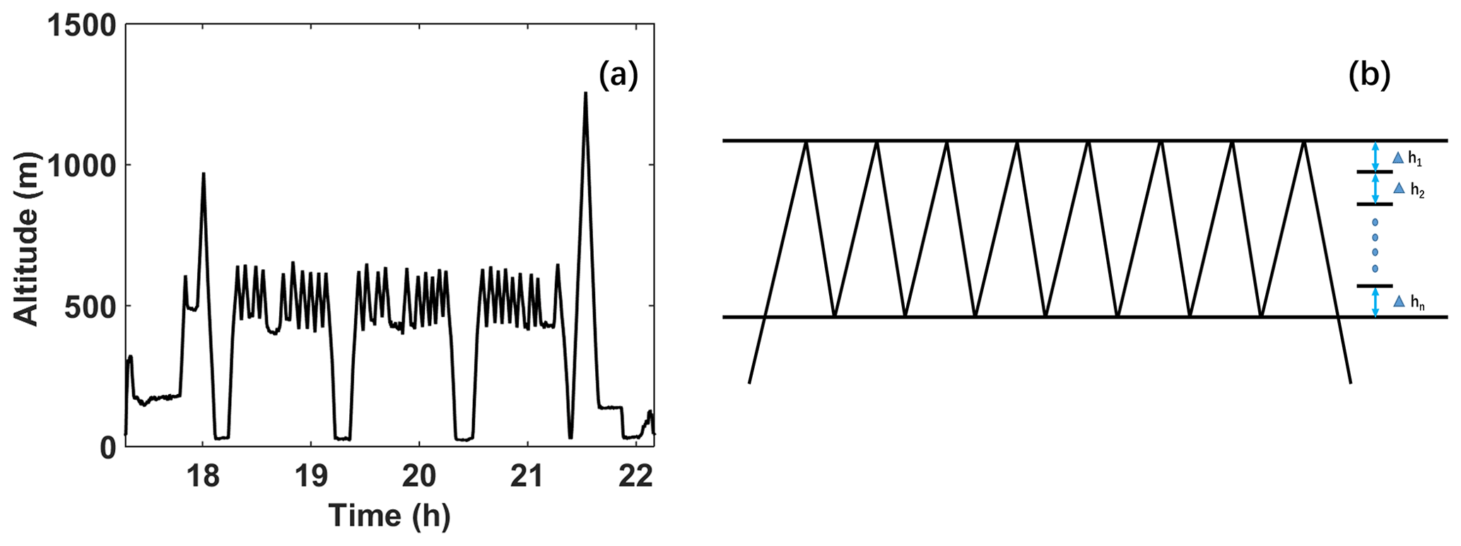
Figure 1(a) Flight track on 16 July 2008. (b) Altitude stratification procedure of the sawtooth patterns, with the mean vertical resolution of 5 m such that m.
2.3 Methods
2.3.1 Existing microphysical measures of homogeneous mixing degree
Based on the diagram of microphysical mixing, four HMDs have been defined to contain all kinds of entrainment-mixing mechanisms. The first three measures are based on the diagram of vs. (Lu et al., 2014a, 2013b), as shown in Fig. 2a and b. Figure 2a declares the various statuses during a whole process of entrainment mixing for defining the first measure (ψ1). The adiabatic cloud is represented by Point A with the number concentration (na) and volume mean radius (rva) of adiabatic state. After environmental air is entrained into cloud, the state of the cloud approaches Point B, whose number concentration is nh and volume mean radius is rva. Then mixing and evaporation processes occur and cloud state approaches Point C, where number concentration after evaporation is nc and volume mean radius after evaporation is rvc. The included angle between the line connecting Point B to Point E and the extreme IM mixing line is , and the included angle between the line connecting Point B to Point C and the extreme IM mixing line is β. Then ψ1 is defined as
where β is
and χ represent the adiabatic cloud fraction after mixing derived from energy conservation and total water conservation in the isobaric mixing (Lehmann et al., 2009; Gerber et al., 2008; Lu et al., 2012). The second HMD (ψ2) is defined in view of Fig. 1b:
where
and
Here, ni is the number concentration after extreme IM mixing and rvh is the volume mean radius after HM mixing. The third measure of HMD (ψ3) is given by
The fourth measure (ψ4) is defined using mixing diagram of vs. LWCLWCa (Lu et al., 2014b), as shown in Fig. 2c:
The definitions of Points A–E are the same as those in Fig. 2a and b. Four kinds of HMDs are expected to range from 0 to 1; the higher probability of HM mixing corresponds to the larger HMD value.
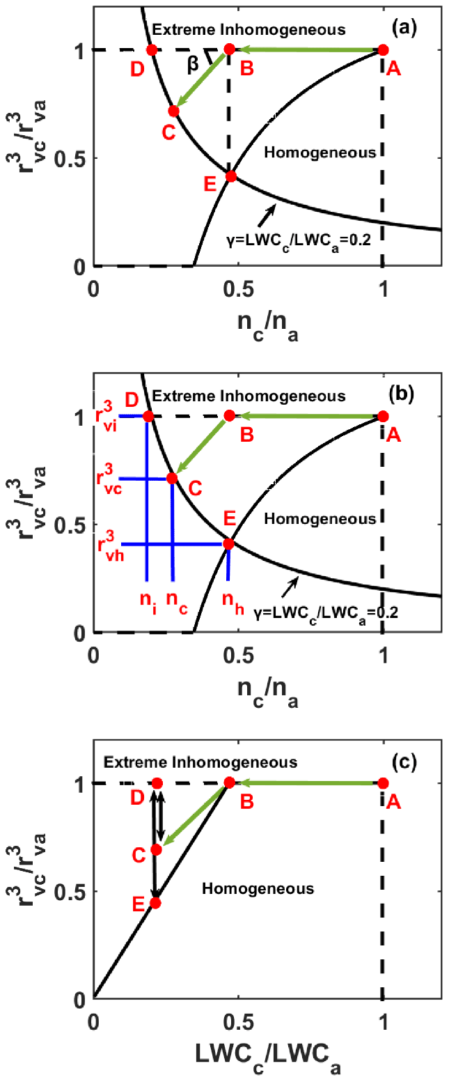
Figure 2Microphysical diagram interpreting the definition for different homogeneous mixing degrees (a ψ1; b ψ2, ψ3; c ψ4). Points A and B represent the adiabatic state and the state after entrainment, respectively. If the extreme inhomogeneous mixing process occurs, the cloud state approaches Point D; if the homogeneous mixing process occurs, the cloud state approaches Point E. The actual mixing and evaporation processes are between the two extremes and cloud state approaches Point C. The extreme inhomogeneous mixing process is represented by the horizontal dashed line; the homogeneous mixing process is represented by the solid line starting from Point A in panels (a) and (b), and the solid line starting from Point B in panel (c). Another black line in panels (a) and (b) corresponds to contour of γ=0.2, defined as the ratio of liquid water content (LWCc) to its adiabatic value (LWCa). See text for the meanings of other symbols.
2.3.2 Definition of a new microphysical measure of homogeneous mixing degree
A new dimensionless HMD (ψ5) is introduced to quantify the different entrainment-mixing mechanisms:
where dis represents the relative standard deviation expressed by the ratio of standard deviation to the average value over each level. During entrainment-mixing and evaporation processes, LWCc always decreases but rvc decreases in the HM mixing and remains constant in the extreme IM mixing. Therefore, the extreme IM mixing corresponds to ψ5=0, and the larger the value of ψ5, the more HM the entrainment mixing. More discussions on ψ5 are given in Sect. 3.2.
2.3.3 Dynamical measures of homogeneous mixing degree
The dynamical aspect, i.e., the mixing process between cloud and environment air vs. the evaporation process of cloud droplets, is important for distinguishing different entrainment-mixing mechanisms (Baker et al., 1980; Baker and Latham, 1979). The mixing timescale divided by evaporation timescale is defined as the Damköhler number (Da), which is usually used to quantify whether the mixing process or evaporation process is faster and thus to discern the entrainment-mixing mechanisms (Siebert et al., 2006; Burnet and Brenguier, 2007; Andrejczuk et al., 2009):
where τmix and τr are the turbulent mixing time and microphysical response time of droplets, respectively (Lehmann et al., 2009). A more IM mixing corresponds to a larger Da. Three kinds of microphysical timescales – phase relaxation time (τphase) (Kumar et al., 2013, 2012), evaporation time (τevap) (Andrejczuk et al., 2009; Baker et al., 1980; Burnet and Brenguier, 2007), and reaction time (τreact) (Lehmann et al., 2009; Lu et al., 2011, 2013c, 2014b) – have been used to represent τr. Lu et al. (2018) found that the most appropriate timescale was τevap if we focus on the changes of number concentration and radius of droplets. The mixing timescale is defined as follows:
where ε is the turbulent dissipation rate calculated from the three-dimensional wind velocities (Meischner et al., 2001) (see Appendix A for details), and L is the size of droplet-free air calculated with
where droplet-free sample size divided by the sum of cloud and droplet-free sample size is considered the fraction of droplet-free F in each vertical interval (e.g., if there are 90 cloud samples and 10 non-cloudy samples, %); TAS and f are the aircraft true air speed (∼ 55 m s−1) and sampling frequency (10 Hz), respectively. The size of droplet-free air is used as a proxy for the entrained air parcels' size. In Eq. (8), the timescale for a droplet of radius rva to completely evaporate (evaporate time) is given by
where S0 is the supersaturation of the droplet-free air at the corresponding altitude (Yau and Rogers, 1996); A is affected by air temperature and pressure (see Appendix B for details).
Another dynamical measure given by the ratio of L* to η is the transition scale number (NL) (Lu et al., 2011):
where transition length (L*) is considered as the corresponding L value when Da=1 (Lehmann et al., 2009) and is given as follows:
In Eq. (12), η is the Kolmogorov length scale (Wyngaard, 2010), which is given by
where v is the kinematic viscosity (Wyngaard, 2010). A higher probability of HM mixing corresponds to a larger value of NL.
3.1 Entrainment-mixing mechanisms from the microphysical and dynamical perspectives
It has been known that it can be uncertain and even problematic to determine the representative adiabatic values from the observational data needed in calculation of the above-mentioned microphysical measures (Yeom et al., 2017; Jensen et al., 1985; Yum et al., 2015). For example, because vertical velocity and concentration of cloud condensation nuclei can change spatially in clouds, na and rva change accordingly. Entrainment mixing in clouds adds difficulties to determine accurate values of rva, na and LWCa. Improper estimation of adiabatic values may violate the theoretical expectation: and rva≥rv, and then cause unrealistic HMDs. Different adiabatic variables have been used in previous studies. For example, the maximum volume mean radius and number concentration are used as proxy values for rva and na for each horizontal penetration, respectively (Yeom et al., 2017; Yum et al., 2015); LWCa is calculated from the adiabatic growth from cloud base, and the maximum number concentration of whole flight penetration is considered as na (Burnet and Brenguier, 2007; Lehmann et al., 2009); na is the mean value of top 2 % of nc for each flight and rva is calculated using adiabatic water vapor mixing ratio, adiabatic total water mixing ratio and na for a horizontal penetration (Small et al., 2013).
Table 1List of different methods determining adiabatic values.
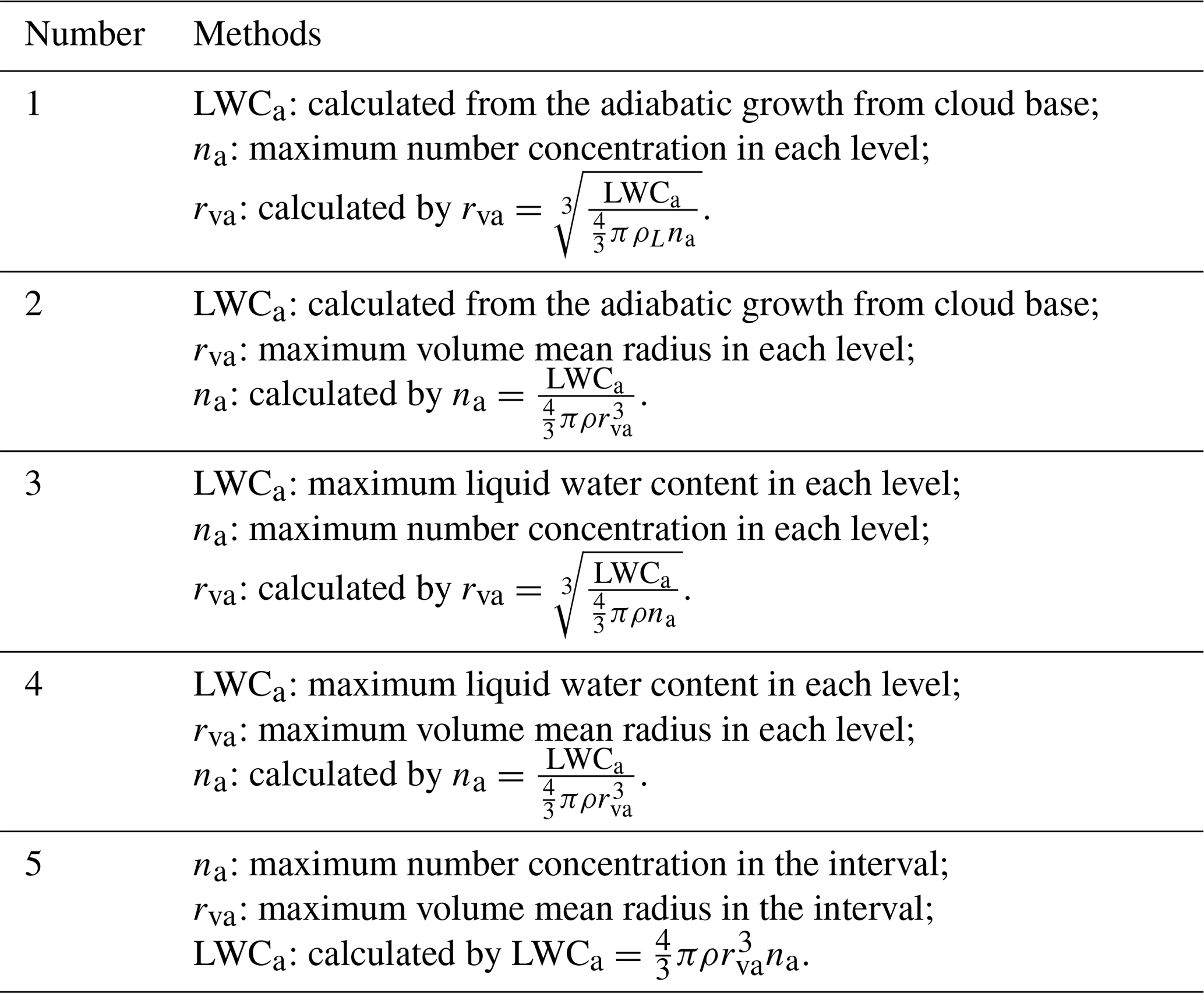
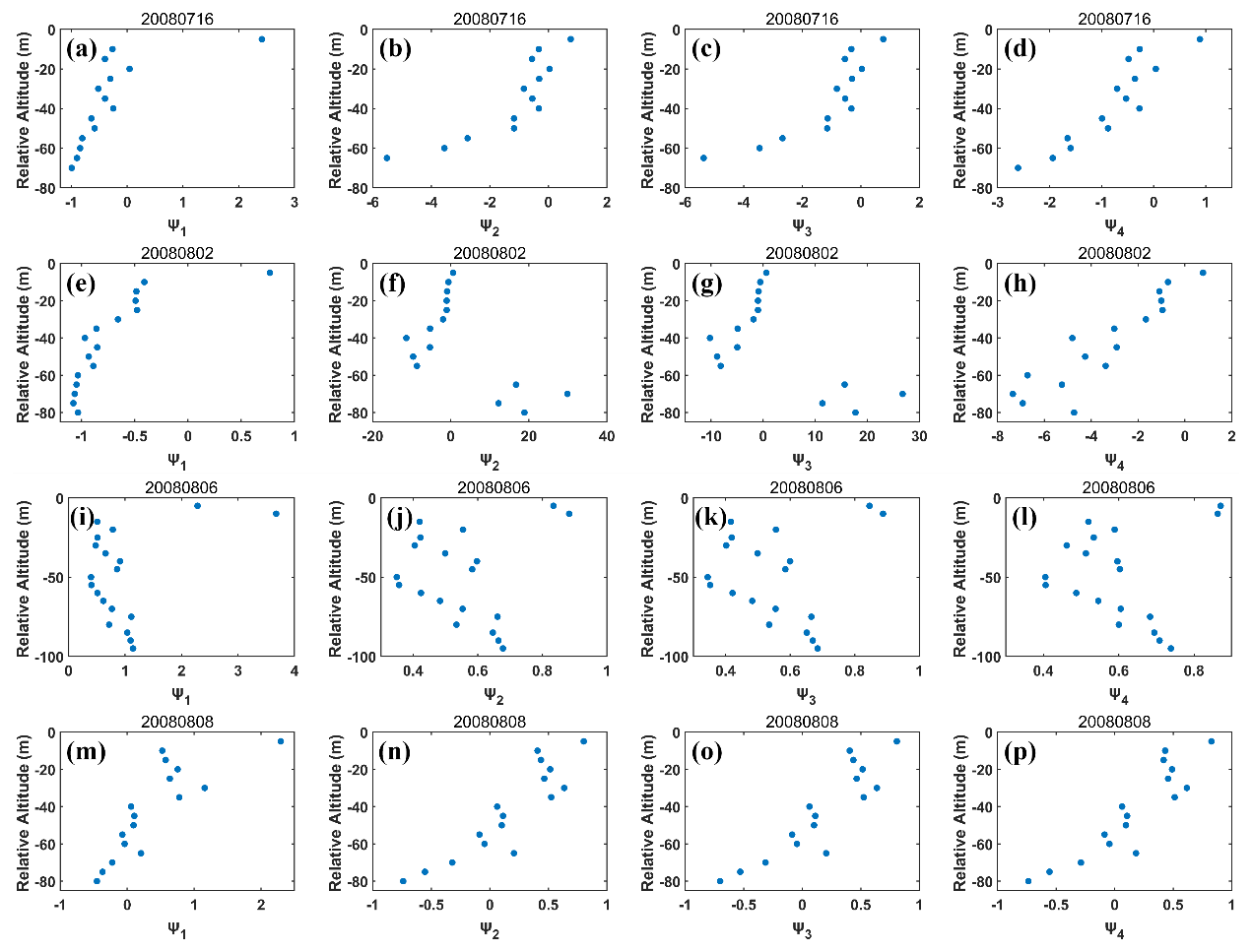
Figure 3Height dependence of the first homogeneous mixing degree (ψ1) on (a) 16 July 2008, (e) 2 August 2008, (i) 6 August 2008 and (m) 8 August 2008; height dependence of the second homogeneous mixing degree (ψ2) on (b) 16 July 2008, (f) 2 August 2008, (j) 6 August 2008 and (n) 8 August 2008; height dependence of the third homogeneous mixing degree (ψ3) on (c) 16 July 2008, (g) 2 August 2008, (k) 6 August 2008 and (o) 8 August 2008; and the fourth homogeneous mixing degree (ψ4) on (d) 16 July 2008, (h) 2 August 2008, (l) 6 August 2008 and (p) 8 August 2008. The relative altitude on the y axis equal to 0 represents the cloud tops. Adiabatic liquid water content (LWCa) is obtained by the adiabatic growth from cloud base, adiabatic number concentration (na) is assumed to be the maximum volume mean radius at each level, and adiabatic volume mean radius (rva) is calculated with LWCa and rva.
To examine the influence of using different adiabatic properties, we compare ψi (i=1–4) calculated with different adiabatic variables (Table 1) at each level near the stratiform cloud tops for the data collected during the four flights. Only the results for the first microphysical measure are shown in Fig. 3; the other results are shown in the Supplement. In Fig. 3, LWCa is based on the adiabatic growth from cloud base, the maximum number concentration at each level is assumed as na, and rva is calculated from LWCa and na. In Fig. S1 in the Supplement, LWCa is based on the adiabatic growth from cloud base, the maximum volume mean radius at each level is assumed as rva, and na is calculated from LWCa and rva. In Fig. S2 in the Supplement, the maximum liquid water content at each level is assumed as LWCa, the maximum number concentration at each level is assumed as na, and rva is calculated from LWCa and na. In Fig. S3 in the Supplement, the maximum liquid water content at each level is assumed as LWCa, the maximum volume mean radius at each level is assumed as rva, and na is calculated from LWCa and rva. In Fig. S4 in the Supplement, the maximum number concentration at each level is assumed as na, the maximum volume mean radius at each level is assumed as rva, and LWCa is calculated from na and rva. According to the definitions, ψi (i=1–4) values are expected to range from 0 to 1. However, some values of ψi (i=1–4) are larger than 1 or smaller than 0 in Figs. 3 and S1–S4, which could be caused by uncertainties in rva, LWCa, na and cloud base (Lu et al., 2014b, a, 2013b; Gerber et al., 2008). Furthermore, these figures suggest different vertical distributions of HMDs for the same flight, suggesting that high sensitivity of the conventional HMDs to the methods for determining the adiabatic values could pose a serious problem as to which figure represents the reality of entrainment-mixing mechanisms.
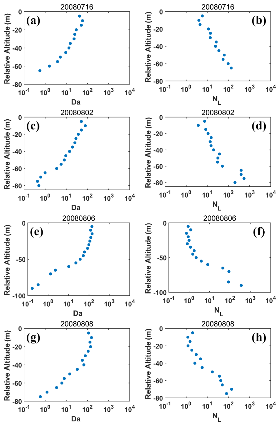
Figure 4Height dependence of Damköhler number (Da) on (a) 16 July 2008, (c) 2 August 2008, (e) 6 August 2008 and (g) 8 August 2008; height dependence of transition scale number (NL) on (b) 16 July 2008, (d) 2 August 2008, (f) 6 August 2008 and (h) 8 August 2008. The relative altitude on the y axis equal to 0 represents the cloud tops. Adiabatic liquid water content (LWCa) is obtained by the adiabatic growth from cloud base, adiabatic number concentration (na) is assumed to be the maximum volume mean radius at each level, and adiabatic volume mean radius (rva) is calculated with LWCa and rva.
Since the above analysis from the microphysical perspective does not tell a consistent story about the vertical variation of HMD, Da and NL are examined from the dynamical perspective. Figure 4a, c, e and g show the height dependence of Da during each of the four flights. It is obvious that Da decreases with decreasing altitudes. Figure 4b, d, f and h show a significant increasing trend of NL with decreasing altitudes. The method for setting the adiabatic values in Fig. 4 is the same as that in Fig. 3; i.e., LWCa is based on the adiabatic growth from cloud base, the maximum number concentration at each level is assumed as na, and rva is calculated from LWCa and na. Unlike the microphysical measures, vertical variations of Da or NL are similar when different methods for determining adiabatic values are used (Figs. S5–S8 in the Supplement). It is expected that a smaller Da (larger NL) represents a larger HMD. The results of Da and NL both suggest more IM mixing closer to cloud top. It is noteworthy that this result is robust, not affected by the methods for obtaining the adiabatic values, and thus should reflect the real height dependence of entrainment-mixing mechanisms.
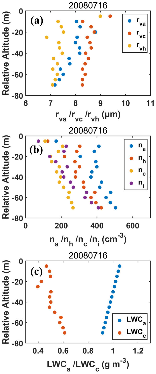
Figure 5Height dependence of (a) rva, rvc, rvh, (b) na, nh, nc, ni and (c) LWCa, LWCc on 16 July 2008. The relative altitude on the y axis equal to 0 represents the cloud tops. Adiabatic liquid water content (LWCa) is obtained by the adiabatic growth from cloud base, the maximum number concentration at each level is assumed to be adiabatic number concentration (na), and adiabatic volume radius (rva) is calculated with LWCa and na.
The different vertical distributions of HMDs and the inconsistency between microphysical HMDs and dynamical measures are mainly due to the improper estimations of adiabatic values. For example, during the flight of 16 July in Fig. 3, the HMDs decrease with the decreasing altitudes, and most of the HMDs are negative. The negative values do not meet the theoretical expectations, and these trends are completely inconsistent with those of dynamical measures. The vertical variations of some important properties of this case are shown in Fig. 5. The negative values of HMDs are due to unexpected result of rva≤rvc. Under these circumstances, the difference between rvc and rva becomes larger with the decreasing altitudes, corresponding to the decreasing trends of HMDs with the decreasing altitudes. Besides the first method, the other four methods mentioned above also have their own unreasonable points. For example, rva≤rvc exists under methods 1, 3 and 4; na≤nc exists under methods 2 and 4; rva does not always increase with the increasing altitudes under methods 2, 4 and 5 (See Figs. S9 to S13 in the Supplement for details). Overall, the inconsistency among the microphysical HMDs estimated with different methods to determine the adiabatic variables calls for a new microphysical measure of entrainment-mixing mechanisms.
3.2 New microphysical measure
As discussed in Sect. 3.1, the existing microphysical measures of HMDs depend on the different adiabatic values to a great extent. In order to avoid this kind of uncertainty, a new dimensionless HMD (ψ5) in Eq. (7) is introduced to quantify the different entrainment-mixing mechanisms. To make sure that ψ5 is applied properly, the correlation between and LWCc must be positive. If the correlation is negative, IM mixing with subsequent ascent is likely to occur (Lu et al., 2013a; Lehmann et al., 2009; Wang et al., 2009; Siebert et al., 2006; Lasher-trapp et al., 2005). It is worth mentioning that ψ5 does not require using adiabatic values and thus can overcome the deficiencies of ψi (i=1–4) associated with choosing different adiabatic cloud properties.
The vertical variations of ψ5 for the four flights are shown in Fig. 6. The small value of ψ5 near the cloud tops shows that entrainment mixing approaches extreme IM, consistent with conclusions in several previous studies based on the POST data (Gerber et al., 2013, 2016; Malinowski et al., 2013). The increase of ψ5 with decreasing altitudes indicates that the trends towards more HM with the decreasing altitudes, consistent with the results of Da and NL (Figs. 4 and S5–S8). We also check the relationship between and LWCc and the two quantities are positively correlated (not shown).
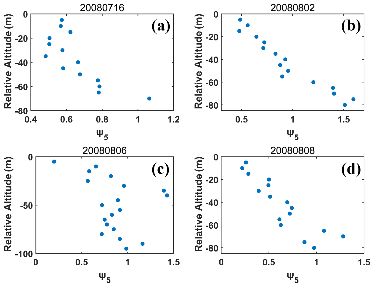
Figure 6Height dependence of the newly defined homogeneous mixing degree (ψ5) on (a) 16 July 2008, (b) 2 August 2008, (c) 6 August 2008 and (d) 8 August 2008. The relative altitude on the y axis equal to 0 represents the cloud tops.
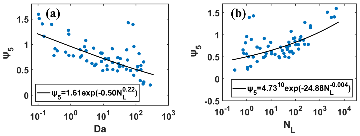
Figure 7Relationships of the newly defined homogeneous mixing degree (ψ5) vs. (a) Damköhler number (Da) and (b) transition scale number (NL).
The relationships between ψ5 vs. Da and NL of the four flights are shown in Fig. 7 and are well fitted by the equations used in Luo et al. (2020):
where the parameters a1 and a2 are positive; b1 and b2 are negative; c1 is positive and c2 is negative. The negative correlation of ψ5 vs. Da and positive correlation of ψ5 vs. NL are evident and in keeping with theoretical arguments, suggesting that a smaller Da or a larger NL corresponds to a higher ψ5. Such relationships further confirm the utility and applicability of ψ5 in studying entrainment-mixing mechanisms. The correlation coefficients of the linear regression of for ψ5 vs. Da and ψ5 vs. NL are about 0.66 and 0.60, respectively, suggesting that Da and NL are basically equivalent for understanding the entrainment-mixing parameterization.

Figure 8Relationships of Damköhler number (Da) vs. transition scale number (NL) on (a) 16 July 2008, (b) 2 August 2008, (c) 6 August 2008 and (d) 8 August 2008.

Figure 9Relationships of transitional scale (L*) vs. droplet-free air length (L) on (a) 16 July 2008, (b) 2 August 2008, (c) 6 August 2008 and (d) 8 August 2008.
The equivalence of Da and NL is further supported by the tight negative correlation between Da and NL (Fig. 8). Similar results have been reported in Gao et al. (2018) using numerical simulations, and Desai et al. (2021) based on holographic measurements. However, the underlying reasons are different. Figure 9 shows that L and L* are negatively correlated, in contrast to the positive correlation between L* and the Taylor microscale in Gao et al. (2018); the Taylor microscale is used as L in the calculation of τmix in Eq. (9) in Gao et al. (2018). It is easy to derive from Eqs. (8), (9), (11) and (12) that , others being equal:
Therefore, as long as L and L* are nearly linearly correlated, Da and NL are equivalent. When extreme IM mixing dominates near the cloud top, ε is small (Fig. 10), which mainly determines small L*; L is large near the cloud top (Fig. 10). Therefore, L and L* are negatively correlated. The vertical distributions of affecting factors on entrainment mixing are detailed in the next subsection.
3.3 Further analysis of affecting factors
According to the analyses in Sect. 3.1 and 3.2, the dynamical and microphysical measures both indicate that entrainment-mixing mechanisms change from IM to HM with decreasing altitudes. Here, we provide the physical explanation for such behavior under the framework of HM/IM entrainment-mixing mechanisms, by analyzing the vertical variations of all the variables defining Da and NL, i.e., ε, relative humidity (RH) and L.
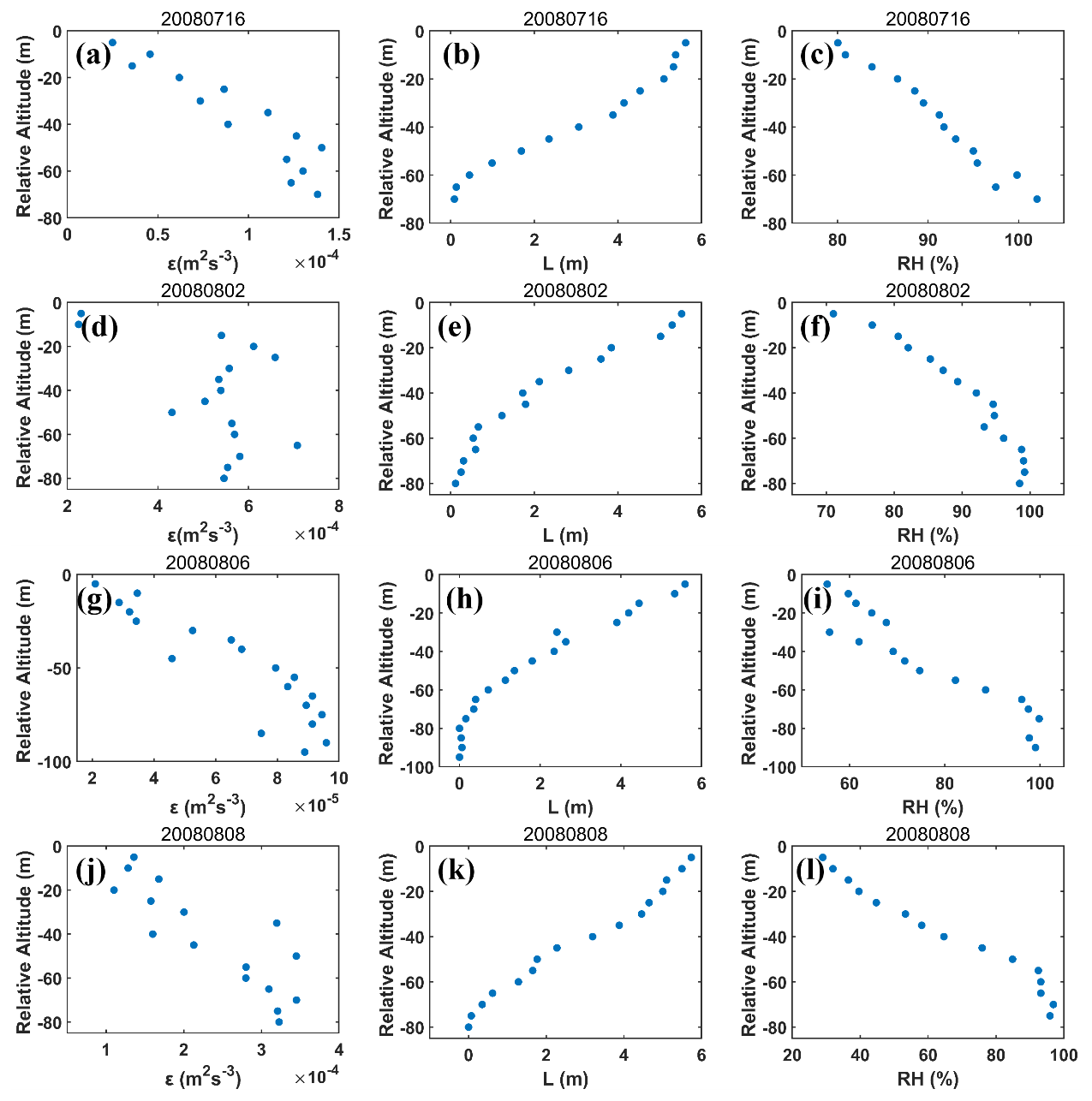
Figure 10Height dependence of dissipation rate (ε) on (a) 16 July 2008, (d) 2 August 2008, (g) 6 August 2008 and (j) 8 August 2008; height dependence of relative humidity (RH) of droplet-free air on (b) 16 July 2008, (e) 2 August 2008, (h) 6 August 2008 and (k) 8 August 2008; and height dependence of length of droplet-free air (L) on (c) 16 July 2008, (f) 2 August 2008, (i) 6 August 2008 and (l) 8 August 2008. The relative altitude on the y axis equal to 0 represents the cloud tops.
First, Fig. 10a, d, g and j show that ε increases with decreasing altitudes, which is opposite to that for cumulus clouds (Small et al., 2013 and Jarecka et al., 2013). According to definition of Da (Eq. 8) and NL (Eq. 12), the increase of ε leads to the decrease of Da and increase of NL, others being equal. Therefore, ε is an important factor to cause Da to decrease and NL to increase with the decreasing altitudes (Figs. 4 and S5–S8). The clouds were sampled in the vicinity of the coast of Santa Cruz/Monterey, California; therefore, these clouds were well mixed and coupled, which explains the monotonic decrease of ε with the increasing height (Jones et al., 2011; Shupe et al., 2013). Note that the decoupled clouds should be very common in the downstream regions (Bretherton and Wyant, 1997) and midlatitudes (Zheng et al., 2020). The boundary layer decoupling causes a decrease of turbulent kinetic energy near the cloud base, leading to a local minimum near the cloud base and a maximum in the middle of cloud layer which can be used to infer the profile of ε (Stevens, 2000). This is also demonstrated in the observations by Zheng et al. (2016), who found a significant role of decoupling in weakening the cloud-base updrafts. Therefore, in the future studies of decoupled stratocumulus in other regions, the results about entrainment-mixing mechanisms could be different due to the non-monotonic vertical variation of ε.
Second, the vertical variation of entrainment mixing can also be attributed to that of entrained air sizes. Figure 10b, e, h and k show that L decreases significantly with decreasing altitudes, which leads to a decrease of Da with decreasing altitudes since Da is proportional to τmix, and thus L. The importance of L has rarely been studied in previous literature for height dependence of entrainment mixing. The decrease of L with decreasing altitudes agrees generally with the cascade of breakdown of dry air parcels entrained at the cloud top.
Third, vertical variation of entrained air RH plays a significant part in determining the entrainment-mixing mechanisms. In former literature (Yeom et al., 2017; Lu et al., 2018), RH is commonly assumed to be constant across multiple different altitudes when calculating τevap using . In fact, RH should not be a constant. We determine RH as the mean RH of droplet-free air in each level. Figure 10c, f, i and l show that RH increases with decreasing altitudes due to droplet evaporation. According to the definition of Da, Da decreases with the increase of τevap, and thus decreases with the increase of RH (Eqs. 7 and 10). Equations (10)–(12) show that NL increases with increasing RH. Both Da and NL indicate more HM mixing at a lower altitude. These results suggest that the increases of ε and RH and the decrease of L with decreasing altitudes are in keeping with the variation of entrainment-mixing processes, together playing the primary role in determining the vertical distribution of HMD observed.
It is noted that rva also affects Da and NL through its effect on τevap. However, rva depends on how adiabatic values are estimated in Sect. 3.1 (Figs. S9–S14). Therefore, the vertical variation of rva is not analyzed here. No matter which method is used to determine the adiabatic values, the trends of vertical variation of Da and NL do not change (Sect. 3.1). The vertical variation of Da and NL indicates the dominance of the combined effects of ε, RH and L in determining the vertical variation of entrainment-mixing processes from IM towards HM with decreasing altitudes.
These results are in keeping with the results drawn in Wang et al. (2009) and Yum et al. (2015) in the sense that a trait of IM mixing is prevalent near the cloud top but at mid-levels of clouds a trait of HM mixing becomes dominant, according to the analysis of cloud microphysical relationships at different altitudes of marine stratiform clouds. However, there are big differences in the spatial scale of analysis between our and their studies. We focus on near-cloud-top regions from cloud top to where droplet-free air patches can still be found, mostly less than 100 m from the cloud top (Fig. 3). On the other hand, Yum et al. (2015) and Wang et al. (2009) examined mid-levels of stratiform clouds where there remained no droplet-free air patches as well as near-cloud-top regions. They suggested that the vertical variation of cloud microphysical properties relationships could be caused by vertical circulation of diluted parcels affected by entrainment; the actual mixing near the cloud top might have been IM as Da and NL at this level suggested; as these parcels moved down, the droplets evaporated fast, resulting in cloud microphysical relationships that would be explained as a trait of HM mixing.
The observational data of marine stratiform clouds measured from aircraft during the campaign of Physics of Stratocumulus Top (POST) are used to examine the height dependence of entrainment-mixing mechanisms. The sawtooth penetrations are analyzed to acquire fine information on the vertical structure of entrainment mixing near stratiform cloud tops, from the microphysical and dynamical perspectives. To ensure high vertical resolution, we take 5 m as one altitude distance bin of all sawtooth patterns for the four flights selected in this study.
From the microphysical perspective, the traditional homogeneous mixing degrees vary distinctly with the decreasing altitudes due to different methods for obtaining adiabatic values. In order to overcome this difficulty, a new homogeneous mixing degree describing the distributions of scatters in the mixing diagram is introduced to quantify different entrainment-mixing mechanisms. The new homogeneous mixing degree is introduced by relative standard deviation of cubic volume mean radius divided by relative standard deviation of liquid water content. If the new homogeneous mixing degree is larger, the mixing is more likely to be homogeneous. The new measure increases with the decreasing altitudes, i.e., more homogeneous with decreasing altitudes. This new measure is not affected by the methods for obtaining adiabatic values and shed new light on the study of entrainment-mixing mechanisms.
From the dynamical perspective, the Damköhler number decreases and transition scale number increases with decreasing altitudes. The relationships between the new homogeneous mixing degree vs. Damköhler number and transition scale number are negative and positive, respectively, consistent with theoretical expectations. Therefore, both microphysical and dynamical analyses indicate the trends from inhomogeneous mixing to homogeneous mixing when altitude decreases.
The factors underlying the vertical variation of entrainment-mixing mechanisms are examined, including vertical distributions of dissipation rate, size of droplet-free air and relative humidity in droplet-free air. Dissipation rate increases and droplet-free air size decreases with the decreasing altitudes. Therefore, mixing is faster at the lower altitude and homogeneous mixing is more likely to occur. Relative humidity increases with decreasing altitudes, which indicates that droplets are less likely to be completely evaporated at the lower altitude. The combined effects of the three factors determine the entrainment-mixing vertical evolution.
It is noteworthy that the traditional homogeneous mixing degrees are still useful properties to quantify entrainment-mixing mechanisms, if adiabatic values of microphysical properties are properly determined. The new homogeneous mixing degree defined here is a relative measure of homogeneous mixing degree as a deviation from the extremely inhomogeneous mixing line but does not quantify the amount of homogeneous mixing precisely. The relative dispersion of volume-mean radius and liquid water content increases due to differences in mixing states (Khain et al., 2018) and in-cloud activation of cloud condensation nuclei (Derksen et al., 2009; Khain et al., 2018), which affects the calculation of the new homogeneous mixing degree. As pointed out by Khain et al. (2018), the mixing diagram has limitations to analyze entrainment-mixing mechanisms using in situ observations, due to transient mixing states. However, this new measure still provides an alternative method to quantify entrainment-mixing mechanisms, supported by the independent Damköhler and transition scale numbers. This new method can be applied to other datasets with different cloud droplet size probes (e.g., the Forward Scattering Spectrometer Probe, FSSP), since the new definition is based on theoretical understanding of entrainment-mixing mechanisms, which is not limited to the dataset used here. It would be interesting to apply this method to other stratocumulus and cumulus observations in different climate zones.
Turbulent dissipation rate (ε) is calculated by three-dimensional wind velocities (Meischner et al., 2001):
with (Panofsky, 1984). DNN is the local spatial structure function using three wind components and is defined as
where three wind components, east, north and vertical, are represented by u, v and w, respectively; TAS is the aircraft true air speed (∼55 m s−1); t is the time; d is the scale parameter:
where Δt is the time interval, which is set to 0.1 s.
The parameter A in Eq. (10) is
where Rv, Lh, T, K, ρL, D and es(T) are water vapor specific gas constant, latent heat, temperature, coefficient of air thermal conductivity coefficient, liquid water density, water vapor diffusion coefficient in air and vapor pressure of saturation, respectively.
The codes can be accessed by contacting Chunsong Lu via luchunsong110@gmail.com. The POST data are available on https://data.eol.ucar.edu/master_lists/generated/post/, last access: 20 July 2021.
The supplement related to this article is available online at: https://doi.org/10.5194/acp-21-11225-2021-supplement.
SG performed the data analysis and wrote the manuscript. CL proposed the idea, guided this work and modified the manuscript. YL and SSY supervised this work and helped revise the manuscript. JZ and LZ offered help with the data analysis. ND, YM and SW also contributed to the modification of manuscript.
The authors declare that they have no conflict of interest.
Publisher's note: Copernicus Publications remains neutral with regard to jurisdictional claims in published maps and institutional affiliations.
The authors thank the crew of the POST campaign.
This research has been supported by the National Key Research and Development Program of China (grant no. 2019YFA0606803), the Second Tibetan Plateau Scientific Expedition and Research (STEP) program (grant no. 2019QZKK0105), the National Natural Science Foundation of China (grant nos. 41822504, 41775131, 42027804, 42075073 and 41975181), the Innovative Project of Postgraduates in Jiangsu Province in 2020 of Jiangsu (grant no. KYCX20_0933) and the China Scholarship Council. Yangang Liu is supported by the US Department of Energy Atmospheric System Research (ASR) program (grant no. DE-SC00112704) and Solar Energy Technologies Office (SETO) under award no. 33504.
This paper was edited by Jianzhong Ma and reviewed by two anonymous referees.
Andrejczuk, M., Grabowski, W. W., Malinowski, S. P., and Smolarkiewicz, P. K.: Numerical Simulation of Cloud–Clear Air Interfacial Mixing: Homogeneous versus Inhomogeneous Mixing, J. Atmos. Sci., 66, 2493–2500, https://doi.org/10.1175/2009jas2956.1, 2009.
Baker, M. and Latham, J.: The evolution of droplet spectra and the rate of production of embryonic raindrops in small cumulus clouds, J. Atmos. Sci., 36, 1612–1615, 1979.
Baker, M., Corbin, R., and Latham, J.: The influence of entrainment on the evolution of cloud droplet spectra: I. A model of inhomogeneous mixing, Q. J. Roy. Meteor. Soc., 106, 581–598, https://doi.org/10.1002/qj.49710644914, 1980.
Baker, M., Breidenthal, R., Choularton, T., and Latham, J.: The effects of turbulent mixing in clouds, J. Atmos. Sci., 41, 299–304, https://doi.org/10.1175/1520-0469(1984)041<0299:TEOTMI>2.0.CO;2, 1984.
Bony, S. and Dufresne, J. L.: Marine boundary layer clouds at the heart of tropical cloud feedback uncertainties in climate models, Geophys. Res. Lett., 32, L20806, https://doi.org/10.1029/2005GL023851, 2005.
Bretherton, C. S., and Wyant, M. C.: Moisture transport, lower-tropospheric stability, and decoupling of cloud-topped boundary layers, J. Atmos. Sci., 54, 148–167, 1997.
Burnet, F. and Brenguier, J.-L.: Observational study of the entrainment-mixing process in warm convective clouds, J. Atmos. Sci., 64, 1995–2011, https://doi.org/10.1175/JAS3928.1, 2007.
Carman, J. K., Rossiter, D. L., Khelif, D., Jonsson, H. H., Faloona, I. C., and Chuang, P. Y.: Observational constraints on entrainment and the entrainment interface layer in stratocumulus, Atmos. Chem. Phys., 12, 11135–11152, https://doi.org/10.5194/acp-12-11135-2012, 2012.
Cess, R. D., Potter, G., Blanchet, J., Boer, G., Ghan, S., Kiehl, J., Le Treut, H., Li, Z.-X., Liang, X.-Z., and Mitchell, J.: Interpretation of cloud-climate feedback as produced by 14 atmospheric general circulation models, Science, 245, 513–516, https://doi.org/10.1126/science.245.4917.513 1989.
Deng, Z., Zhao, C., Zhang, Q., Huang, M., and Ma, X.: Statistical analysis of microphysical properties and the parameterization of effective radius of warm clouds in Beijing area, Atmos. Res., 93, 888–896, 2009.
Derksen, J. W. B., Roelofs, G.-J. H., and Röckmann, T.: Influence of entrainment of CCN on microphysical properties of warm cumulus, Atmos. Chem. Phys., 9, 6005–6015, https://doi.org/10.5194/acp-9-6005-2009, 2009.
Desai, N., Liu, Y., Glienke, S., Shaw, R. A., Lu, C., Wang, J., and Gao, S.: Vertical Variation of Turbulent Entrainment Mixing Processes in Marine Stratocumulus Clouds Using High-Resolution Digital Holography, J. Geophys. Res.-Atmos., 126, e2020JD033527, https://doi.org/10.1029/2020JD033527, 2021.
Freud, E., Rosenfeld, D., Andreae, M. O., Costa, A. A., and Artaxo, P.: Robust relations between CCN and the vertical evolution of cloud drop size distribution in deep convective clouds, Atmos. Chem. Phys., 8, 1661–1675, https://doi.org/10.5194/acp-8-1661-2008, 2008.
Freud, E., Rosenfeld, D., and Kulkarni, J. R.: Resolving both entrainment-mixing and number of activated CCN in deep convective clouds, Atmos. Chem. Phys., 11, 12887–12900, https://doi.org/10.5194/acp-11-12887-2011, 2011.
Gao, W., Sui, C. H., Fan, J., Hu, Z., and Zhong, L.: A study of cloud microphysics and precipitation over the Tibetan Plateau by radar observations and cloud-resolving model simulations, J. Geophys. Res.-Atmos., 121, 13735–713752, 2016.
Gao, Z., Liu, Y., Li, X., and Lu, C.: Investigation of turbulent entrainment-mixing processes with a new particle-resolved direct numerical simulation model, J. Geophys. Res.-Atmos., 123, 2194–2214, 2018.
Gerber, H., Frick, G., Malinowski, S. P., Kumala, W., and Krueger, S.: POST – A new look at stratocumulus, American Meteorological Society 13th Conference on Cloud Physics, 2010.
Gerber, H., Frick, G., Malinowski, S. P., Jonsson, H., Khelif, D., and Krueger, S. K.: Entrainment rates and microphysics in POST stratocumulus, J. Geophys. Res.-Atmos., 118, 12094–12109, 2013.
Gerber, H., Malinowski, S. P., and Jonsson, H.: Evaporative and radiative cooling in POST stratocumulus, J. Atmos. Sci., 73, 3877–3884, 2016.
Gerber, H. E., Frick, G. M., Jensen, J. B., and Hudson, J. G.: Entrainment, mixing, and microphysics in trade-wind cumulus, J. Meteorol. Soc. Jpn. Ser. II, 86, 87–106, 2008.
Grabowski, W. W.: Indirect impact of atmospheric aerosols in idealized simulations of convective–radiative quasi equilibrium, J. Climate, 19, 4664–4682, https://doi.org/10.1175/JCLI3857.1, 2006.
Haman, K. E., Malinowski, S. P., Kurowski, M. J., Gerber, H., and Brenguier, J.-L.: Small scale mixing processes at the top of a marine stratocumulus – a case study, Q. J. Roy. Meteor. Soc., 133, 213–226, https://doi.org/10.1002/qj.5, 2007.
Hill, S. A., Krueger, S., Gerber, H., and Malinowski, S.: Entrainment interface layer of stratocumulus-topped boundary layers during POST, 13 AMS Conf. On Cloud Phys., 2010.
Hoffmann, F. and Feingold, G.: Entrainment and Mixing in Stratocumulus: Effects of a New Explicit Subgrid-Scale Scheme for Large-Eddy Simulations with Particle-Based Microphysics, J. Atmos. Sci., 76, 1955–1973, https://doi.org/10.1175/jas-d-18-0318.1, 2019.
Hudson, J. G. and Yum, S. S.: Droplet spectral broadening in marine stratus, J. Atmos. Sci., 54, 2642–2654, https://doi.org/10.1175/1520-0469(1997)054<2642:DSBIMS>2.0.CO;2, 1997.
Jarecka, D., Grabowski, W. W., Morrison, H., and Pawlowska, H.: Homogeneity of the subgrid-scale turbulent mixing in large-eddy simulation of shallow convection, J. Atmos. Sci., 70, 2751–2767, 2013.
Jen-La Plante, I., Ma, Y., Nurowska, K., Gerber, H., Khelif, D., Karpinska, K., Kopec, M. K., Kumala, W., and Malinowski, S. P.: Physics of Stratocumulus Top (POST): turbulence characteristics, Atmos. Chem. Phys., 16, 9711–9725, https://doi.org/10.5194/acp-16-9711-2016, 2016.
Jensen, J., Austin, P., Baker, M., and Blyth, A.: Turbulent mixing, spectral evolution and dynamics in a warm cumulus cloud, J. Atmos. Sci., 42, 173–192, https://doi.org/10.1175/1520-0469(1985)042<0173:TMSEAD>2.0.CO;2, 1985.
Jones, C. R., Bretherton, C. S., and Leon, D.: Coupled vs. decoupled boundary layers in VOCALS-REx, Atmos. Chem. Phys., 11, 7143–7153, https://doi.org/10.5194/acp-11-7143-2011, 2011.
Khain, A., Pinsky, M., and Magaritz-Ronen, L.: Physical interpretation of mixing diagrams, J. Geophys. Res.-Atmos., 123, 529–542, 2018.
Kumala, W., Haman, K. E., Kopec, M. K., Khelif, D., and Malinowski, S. P.: Modified ultrafast thermometer UFT-M and temperature measurements during Physics of Stratocumulus Top (POST), Atmos. Meas. Tech., 6, 2043–2054, https://doi.org/10.5194/amt-6-2043-2013, 2013.
Kumar, B., Janetzko, F., Schumacher, J. R., and Shaw, R. A.: Extreme responses of a coupled scalar–particle system during turbulent mixing, New J. Phys., 14, 115020, https://doi.org/10.1088/1367-2630/14/11/115020, 2012.
Kumar, B., Schumacher, J., and Shaw, R. A.: Cloud microphysical effects of turbulent mixing and entrainment, Theor. Comput. Fluid Dyn., 27, 361–376, https://doi.org/10.1007/s00162-012-0272-z, 2013.
Kumar, B., Götzfried, P., Suresh, N., Schumacher, J., and Shaw, R. A.: Scale Dependence of Cloud Microphysical Response to Turbulent Entrainment and Mixing, J. Adv. Model. Earth Sy., 10, 2777–2785, 2018.
Lasher-trapp, S. G., Cooper, W. A., and Blyth, A. M.: Broadening of droplet size distributions from entrainment and mixing in a cumulus cloud, Q. J. Roy. Meteor. Soc. A, 131, 195–220, https://doi.org/10.1256/qj.03.199, 2005.
Lehmann, K., Siebert, H., and Shaw, R. A.: Homogeneous and Inhomogeneous Mixing in Cumulus Clouds: Dependence on Local Turbulence Structure, J. Atmos. Sci., 66, 3641–3659, https://doi.org/10.1175/2009jas3012.1, 2009.
Liu, Y., Daum, P. H., Chai, S. K., and Liu, F.: Cloud parameterizations, cloud physics, and their connections: an overview, Brookhaven National Lab., Upton, NY, US, 2002.
Lu, C., Liu, Y., and Niu, S.: Examination of turbulent entrainment-mixing mechanisms using a combined approach, J. Geophys. Res.-Atmos., 116, D20207, https://doi.org/10.1029/2011JD015944, 2011.
Lu, C., Liu, Y., Niu, S., and Vogelmann, A. M.: Lateral entrainment rate in shallow cumuli: Dependence on dry air sources and probability density functions, Geophys. Res. Lett., 39, L20812, https://doi.org/10.1029/2012GL053646, 2012.
Lu, C., Liu, Y., and Niu, S.: A method for distinguishing and linking turbulent entrainment mixing and collision-coalescence in stratocumulus clouds, Chinese Sci. Bull., 58, 545–551, 2013a.
Lu, C., Liu, Y., Niu, S., Krueger, S., and Wagner, T.: Exploring parameterization for turbulent entrainment-mixing processes in clouds, J. Geophys. Res.-Atmos., 118, 185–194, 2013b.
Lu, C., Niu, S., Liu, Y., and Vogelmann, A. M.: Empirical relationship between entrainment rate and microphysics in cumulus clouds, Geophys. Res. Lett., 40, 2333–2338, https://doi.org/10.1002/grl.50445, 2013c.
Lu, C., Liu, Y., and Niu, S.: Entrainment-mixing parameterization in shallow cumuli and effects of secondary mixing events, Chinese Sci. Bull., 59, 896–903, https://doi.org/10.1007/s11434-013-0097-1, 2014a.
Lu, C., Liu, Y., Niu, S., and Endo, S.: Scale dependence of entrainment-mixing mechanisms in cumulus clouds, J. Geophys. Res.-Atmos., 119, 13877–813890, https://doi.org/10.1002/2014jd022265, 2014b.
Lu, C., Liu, Y., Zhu, B., Yum, S. S., Krueger, S. K., Qiu, Y., Niu, S., and Luo, S.: On Which Microphysical Time Scales to Use in Studies of Entrainment-Mixing Mechanisms in Clouds, J. Geophys. Res.-Atmos., 123, 3740–3756, 2018.
Luo, S., Lu, C., Liu, Y., Bian, J., Gao, W., Li, J., Xu, X., Gao, S., Yang, S., and Guo, X.: Parameterizations of Entrainment-Mixing Mechanisms and Their Effects on Cloud Droplet Spectral Width Based on Numerical Simulations, J. Geophys. Res.-Atmos., 125, e2020JD032972, https://doi.org/10.1029/2020JD032972, 2020.
Ma, Y.-F., Malinowski, S. P., Karpińska, K., Gerber, H. E., and Kumala, W.: Scaling analysis of temperature and liquid water content in the marine boundary layer clouds during POST, J. Atmos. Sci., 74, 4075–4092, 2017.
Ma, Y. F., Pedersen, J., Grabowski, W., Kopec, M., and Malinowski, S.: Influences of Subsidence and Free-Tropospheric Conditions on the Nocturnal Growth of Nonclassical Marine Stratocumulus, J. Adv. Model. Earth Sy., 10, 2706–2730, 2018.
Malinowski, S. P., Haman, K., Kumula, W., Kopec, M., Gerber, H., and Krueger, S.: Smallscale variability of temperature and LWC at stratocumulus top, 13 AMS Conf. On Cloud Phys., 27 June–2 July 2010, Portland, 2010.
Malinowski, S. P., Gerber, H., Jen-La Plante, I., Kopec, M. K., Kumala, W., Nurowska, K., Chuang, P. Y., Khelif, D., and Haman, K. E.: Physics of Stratocumulus Top (POST): turbulent mixing across capping inversion, Atmos. Chem. Phys., 13, 12171–12186, https://doi.org/10.5194/acp-13-12171-2013, 2013.
Meischner, P., Baumann, R., and Holler, H.: Eddy Dissipation Rates in Thunderstorms Estimated by Doppler Radar in Relation to Aircraft In Situ Measurements, J. Atmos. Ocean. Tech., 18, 1609–1627, 2001.
Morrison, A. G.: Advanced Two-Moment Bulk Microphysics for Global Models. Part I: Off-Line Tests and Comparison with Other Schemes, J. Climate, 28, 1288–1307, 2015.
Panofsky, H. A.: Atmospheric turbulence, Models and methods for engineering applications, John Wiley, New York, 397, 1984.
Pawlowska, H., Brenguier, J., and Burnet, F.: Microphysical properties of stratocumulus clouds, Atmos. Res., 55, 15–33, https://doi.org/10.1016/S0169-8095(00)00054-5, 2000.
Shupe, M. D., Persson, P. O. G., Brooks, I. M., Tjernström, M., Sedlar, J., Mauritsen, T., Sjogren, S., and Leck, C.: Cloud and boundary layer interactions over the Arctic sea ice in late summer, Atmos. Chem. Phys., 13, 9379–9399, https://doi.org/10.5194/acp-13-9379-2013, 2013.
Siebert, H., Franke, H., Lehmann, K., Maser, R., Saw, E. W., Schell, D., Shaw, R. A., and Wendisch, M.: Probing finescale dynamics and microphysics of clouds with helicopter-borne measurements, B. Am. Meteorol. Soc, 87, 1727–1738, 2006.
Small, J. D., Chuang, P. Y., and Jonsson, H. H.: Microphysical imprint of entrainment in warm cumulus, Tellus B, 65, 19922, 2013.
Stephens, G. L.: Cloud feedbacks in the climate system: A critical review, J. Climate, 18, 237–273, https://doi.org/10.1175/JCLI-3243.1, 2005.
Stevens, B.: Cloud transitions and decoupling in shear-free stratocumulus-topped boundary layers, Geophys. Res. Lett., 27, 2557–2560, 2000.
Su, C.-W., Krueger, S. K., McMurtry, P. A., and Austin, P. H.: Linear eddy modeling of droplet spectral evolution during entrainment and mixing in cumulus clouds, Atmos. Res., 47, 41–58, https://doi.org/10.1016/S0169-8095(98)00039-8, 1998.
Telford, J.: Clouds with turbulence; the role of entrainment, Atmos. Res., 40, 261–282, https://doi.org/10.1016/0169-8095(95)00038-0, 1996.
Telford, J. W. and Chai, S. K.: A new aspect of condensation theory, Pure Appl. Geophys., 118, 720–742, https://doi.org/10.1007/bf01593025, 1980.
Wang, J., Daum, P. H., Yum, S. S., Liu, Y., Senum, G. I., Lu, M.-L., Seinfeld, J. H., and Jonsson, H.: Observations of marine stratocumulus microphysics and implications for processes controlling droplet spectra: Results from the Marine Stratus/Stratocumulus Experiment, J. Geophys. Res., 114, D18210, https://doi.org/10.1029/2008jd011035, 2009.
Wang, Y.: Aerosol-Cloud Interactions from Urban, Regional, to Global Scales, Springer, Burlin, 2015.
Wang, Y., Niu, S., Lv, J., Lu, C., Xu, X., Wang, Y., Ding, J., Zhang, H., Wang, T., and Kang, B.: A new method for distinguishing unactivated particles in cloud condensation nuclei (CCN) measurements: Implications for aerosol indirect effect evaluation, Geophys. Res. Lett., 46, 14185–14194, 2019.
Wood, R.: Stratocumulus clouds, Mon. Weather Rev., 140, 2373–2423, 2012.
Wyngaard, J. C.: Turbulence in the Atmosphere, Cambridge University Press, England, 2010.
Xu, X. and Xue, H.: Impacts of free-tropospheric temperature and humidity on nocturnal nonprecipitating marine stratocumulus, J. Atmos. Sci., 72, 2853–2864, 2015.
Xu, X., Lu, C., Liu, Y., Gao, W., Wang, Y., Cheng, Y., Luo, S., and Weverberg, K. V.: Effects of Cloud Liquid-Phase Microphysical Processes in Mixed-Phase Cumuli Over the Tibetan Plateau, J. Geophys. Res.-Atmos., 125, e2020JD033371, https://doi.org/10.1029/2020JD033371, 2020.
Xue, H. and Feingold, G.: Large-eddy simulations of trade wind cumuli: Investigation of aerosol indirect effects, J. Atmos. Sci., 63, 1605–1622, https://doi.org/10.1175/JAS3706.1, 2006.
Yau, M. K. and Rogers, R. R.: A short course in cloud physics, Elsevier, Oxford, 1996.
Yeom, J. M., Yum, S. S., Liu, Y., and Lu, C.: A study on the entrainment and mixing process in the continental stratocumulus clouds measured during the RACORO campaign, Atmos. Res., 194, 89–99, https://doi.org/10.1016/j.atmosres.2017.04.028, 2017.
Yum, S. S., Wang, J., Liu, Y., Senum, G., Springston, S., McGraw, R., and Yeom, J. M.: Cloud microphysical relationships and their implication on entrainment and mixing mechanism for the stratocumulus clouds measured during the VOCALS project, J. Geophys. Res.-Atmos., 120, 5047–5069, https://doi.org/10.1002/2014jd022802, 2015.
Zhang, Q., Quan, J., Tie, X., Huang, M., and Ma, X.: Impact of aerosol particles on cloud formation: Aircraft measurements in China, Atmos. Environ., 45, 665–672, 2011.
Zhao, C. and Garrett, T. J.: Effects of Arctic haze on surface cloud radiative forcing, Geophys. Res. Lett., 42, 557–564, 2015.
Zheng, Y. and Rosenfeld, D.: Linear relation between convective cloud base height and updrafts and application to satellite retrievals, Geophys. Res. Lett., 42, 6485–6491, 2015.
Zheng, Y., Rosenfeld, D., and Li, Z.: Quantifying cloud base updraft speeds of marine stratocumulus from cloud top radiative cooling, Geophys. Res. Lett., 43, 11407–11413, 2016.
Zheng, Y., Rosenfeld, D., and Li, Z.: A more general paradigm for understanding the decoupling of stratocumulus-topped boundary layers: The importance of horizontal temperature advection, Geophys. Res. Lett., 47, e2020GL087697, https://doi.org/10.1029/2020GL087697, 2020.