the Creative Commons Attribution 4.0 License.
the Creative Commons Attribution 4.0 License.
 | 16 Jul 2021
Measured and modelled air quality trends in Italy over the period 2003–2010
Gino Briganti
Lina Vitali
Antonio Piersanti
Gaia Righini
Massimo D'Isidoro
Andrea Cappelletti
Mihaela Mircea
Mario Adani
Gabriele Zanini
Luisella Ciancarella
Air pollution harms human health and the environment. Several regulatory efforts and different actions have been taken in the last decades by authorities. Air quality trend analysis represents a valid tool in assessing the impact of these actions taken both at national and local levels. This paper presents for the first time the capability of the Italian national chemical transport model, AMS-MINNI, in capturing the observed concentration trends of three air pollutants – NO2, inhalable particles having diameter less than 10 µm (PM10), and O3 – in Italy over the period 2003–2010. We firstly analyse the model performance finding it in line with the state of the art of regional air quality modelling. The modelled trends result in a general significant downward trend for the three pollutants and, in comparison with observations, the values of the simulated trends were of a similar magnitude for NO2 (in the range −3.0 to −0.5 µg m−3 yr−1), while a smaller range of trends was found than those observed for PM10 (−1.5 to −0.5 µg m−3 yr−1) and O3 maximum daily 8 h average concentration (−2.0 to −0.5 µg m−3 yr−1). As a general result, we find good agreement between modelled and observed trends; moreover, the model provides a greater spatial coverage and statistical significance of pollutant concentration trends with respect to observations, in particular for NO2. We also conduct a qualitative attempt to correlate the temporal concentration trends to meteorological and emission variability. Since no clear tendency in yearly meteorological anomalies (temperature, precipitation, geopotential height) was observed for the period investigated, we focus the discussion of concentration trends on emission variations. We point out that, due to the complex links between precursor emissions and air pollutant concentrations, emission reductions do not always result in a corresponding decrease in atmospheric concentrations, especially for those pollutants that are formed in the atmosphere such as O3 and the major fraction of PM10. These complex phenomena are still uncertain and their understanding is of the utmost importance in planning future policies for reducing air pollution and its impacts on health and ecosystems.
- Article
(7290 KB) - Full-text XML
-
Supplement
(1990 KB) - BibTeX
- EndNote


Air pollution represents one of the main environmental challenges of modern society. Numerous studies have already demonstrated the adverse effects on health (Pope et al., 2020; WHO, 2019; Pope and Dockery, 2006; Cohen et al., 2017) and the environment (EEA, 2020; Feng et al., 2019), as well as on climate (Watts et al., 2019; Fuzzi et al., 2015), society, and the economy (Lanzi and Dellink, 2019; OECD, 2016). The adverse impact on health of fine particulate matter results in premature deaths due to ischemic heart disease, strokes, lung cancer, chronic obstructive pulmonary disease, and respiratory infections (Apte et al., 2018; Rajagopalan et al., 2018).
Efforts aimed at reducing air pollution have been ongoing for decades, namely in the framework of the Convention on Long-Range Transboundary Air Pollution drawn up under the United Nations Economic Commission for Europe, leading to a general decrease in air pollutant concentrations in Europe (Maas and Grennfelt, 2016). The trends in concentrations are useful to verify whether and to what degree environmental regulations establishing limits for pollutant emissions, e.g. the Gothenburg protocol (UNECE, 1979) and the European directive on national emission ceilings (EC, 2016), have been effective and efficient in improving air quality at the national and local level. Several European studies addressed this topic, focussing on the entire continent (Colette et al., 2011, 2016, 2017a; Wilson et al., 2012; Guerreiro et al., 2014; Yan et al., 2018) and on single countries (Sicard et al., 2009; Cattani et al., 2014; Querol et al., 2014; Carnell et al., 2019; Velders et al., 2020). The studies were carried out using observed and/or modelled concentrations. The best approach should be the one which integrates both of these sources of information. Indeed, the observed concentrations provide an actual air quality evaluation, though at sparse locations and sometimes with poor temporal coverage, while the modelled concentrations offer a comprehensive spatial and temporal coverage, although they have intrinsic uncertainties in describing the complex processes of atmospheric chemistry and physics (Iversen, 1993).
For Europe, Colette et al. (2011) performed an assessment of nitrogen dioxide (NO2), particulate matter with a diameter of 10 µm or less (PM10), and ozone (O3) concentration trends over the 1998–2007 decade, using six regional and global chemical transport models (CTMs). The simulated trends were evaluated against observed ones at background monitoring stations located in major anthropogenic emission hotspots. This comparison showed that the primary pollutant trends were generally well reproduced by simulations, with lower performance for O3, which is a secondary pollutant produced in the atmosphere. Wilson et al. (2012) also investigated the O3 trends over Europe using the CHIMERE model between 1996 and 2005. The data collected in 158 rural background stations showed that the model reproduces well the European-averaged O3 trend of the annual 5th percentiles but failed to reproduce the positive trend in the observed 95th percentiles. Another European-wide study was conducted by Yan et al. (2018) for the period 1995–2012 using the global chemical transport model EMAC. The results showed that the model successfully captured the observed temporal variability in O3 mean concentrations at EMEP background stations, as well as the contrast in the trends of the 95th percentile (decreasing) and 5th percentile (increasing). Solberg et al. (2015) and Colette et al. (2017b) provided reviews of scientific papers which compare modelled to observed trends in Europe. In the EURODELTA-Trends multi-model exercise at the European scale, Colette et al. (2017a) investigated the period 1990–2010 with eight chemical transport models (including the AMS-MINNI, Atmospheric Modelling System of the Italian National Integrated Model to support the international negotiation on atmospheric pollution; Mircea et al., 2014; Vitali et al., 2019). The authors showed the time variability of PM10, PM2.5 (Tsyro et al., 2017), organic aerosols and precursor gases (Ciarelli et al., 2019), and O3 (Mar et al., 2016; Colette et al., 2017b). In particular, the EURODELTA-Trends study, by analysing emissions, intercontinental inflow, and meteorological variability, confirmed that the reduction in European anthropogenic emissions plays a fundamental role in the modelled net reduction in ambient air pollution.
Italy is affected by air pollution at the highest levels recorded in Europe (EEA, 2020). Despite this evidence, even if the above-mentioned studies over the European area include Italy in their investigations of long-term air quality trends, few analyses focussing on the Italian territory are available. Most of the available trend analyses rely on measured concentrations of single pollutants at single monitoring stations (Casale et al., 2000; Cristofanelli et al., 2015; Gilardoni et al., 2020) or in distinct urban areas (Cadum et al., 1999; Cattani et al., 2010; Gualtieri et al., 2014; Pozzer et al., 2019) and administrative regions (Carugno et al., 2017; Masiol et al., 2017; Lonati and Cernuschi, 2020). Some works cover the whole Po Valley, in northern Italy, which is a well-known regional hotspot for air pollution (Putaud et al., 2014; Bigi and Ghermandi, 2016). Currently, the studies by Cattani et al. (2014, 2018) are the only Italian-wide analyses, and they are based on measured concentrations available from the National Air Quality database (BRACE, 2013). In particular, Cattani et al. (2014) show significant reduction trends in concentrations of carbon monoxide (CO) and benzene (C6H6), linearly related with emission reductions, and a large number of stations measuring decreasing PM10 and NO2 trends and low statistical significance in O3 trends, which indicates that no clear trend exists in measured ozone concentrations. So far, to the present authors' knowledge, there is no modelling study exploring concentration trends and their relations with emission changes over time covering the whole Italian territory.
This paper evaluates the trends of three air pollutants (NO2, PM10, O3) in Italy, over the period 2003–2010, using the AMS-MINNI air quality model. The evaluation of CTM capabilities to reproduce the trends of pollutants increases the reliability of their application in assessing air quality and supporting air quality plans, especially for models regularly used in national regulatory assessments, as requested by air quality (EC, 2008) and national emission ceiling (EC, 2016) directives but also for other scientific studies. The analysis is based on statistical methods widely used in the literature, for the sake of comparability with other investigations on air quality trends. The ability of the model to reproduce the concentration trends is evaluated through the comparison with independent data available from the National Air Quality database (BRACE).
Moreover, in order to identify the potential efficacy of mitigation policies in reducing air pollution, concentration trends were qualitatively compared with variations in meteorology and anthropogenic emissions. Abbreviations are defined in Appendix A.
2.1 Air quality measurements
The air quality monitoring data considered in the present work derive from BRACE, in which data from regional/local monitoring networks were collected for the formal submission to the European Environment Agency (EEA), in the framework of the reciprocal exchange of information and data from networks and individual stations measuring ambient air pollution within the Member States (EC, 1997). BRACE fed the European database Airbase (Airbase, 2020) with data from 2002 to 2012, thus covering the period investigated in this study.
Several processing steps were applied to the raw BRACE database in order to adapt the database to model validation requirements and to verify station reported metadata, in particular concerning geographical coordinates (Piersanti et al., 2012).
In the present work, in order to analyse the concentration trends, we selected only stations covering the 100 % of the investigated years with at least 75 % of valid data per year. The two thresholds for time coverage were chosen according to the legal requirements on yearly time series stated in the Air Quality Directive (EC, 2008) and also widely adopted in scientific literature (Colette et al., 2011, 2016), for a robust analysis. The threshold of 100 % of the investigated years is a more stringent criterion with respect to other studies, generally adopting a less stringent criterion (e.g. 75 % is set in Colette et al., 2011, corresponding in the same cases to 8 years). Our choice guarantees that the trend analysis is always based on an 8-year period, which can be considered quite robust. Indeed, several studies are available in the literature, presenting trend analysis over similar or shorter periods (Zhai et al., 2019; Dufour et al., 2018; Sheng et al., 2018). Of course, data covering a longer period would strengthen our findings. Anyway, in this first study over Italy, the choice of the period to investigate was determined by the availability of coherent model results that have the same model setup for the years 2003 to 2010. More specifically, in the following years, AMS-MINNI simulations adopted a different setup (spatial domain, chemical mechanism, boundary conditions), which clearly affects time series homogeneity. The pollutants considered are NO2, PM10, and O3 due to their large monitoring coverage in the period of interest. Particulate matter with a diameter of less than 2.5 µm (PM2.5) could not be included in the analysis, as the data coverage from BRACE started in 2007 (Uccelli et al., 2017). Time resolution is given in hours (for NO2 and O3) and days (for PM10).
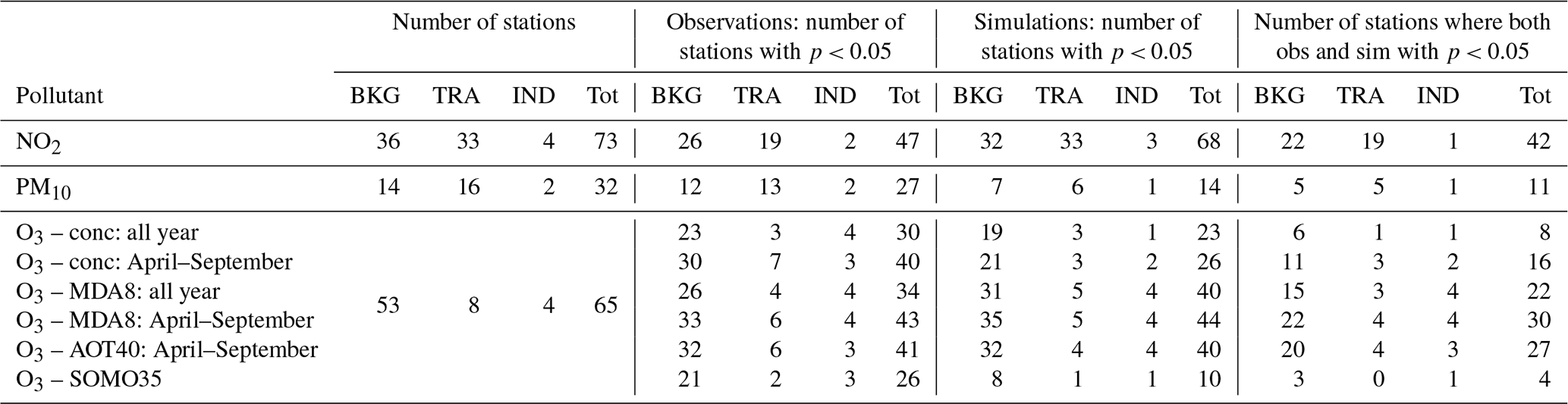
The number of the air quality monitoring stations that satisfied the chosen criteria is reported in Table 2. In Sect. S1 of the Supplement, Fig. S1 represents the 20 Italian administrative regions and Figs. S2–S4 the locations of all sites that passed the selection criteria, by station type (background – BKG, traffic – TRA, industrial – IND) and the background sites by zone type (rural, suburban, urban). The model spatial resolution of 4 km is not sufficient to describe TRA and IND stations with the same skills of BKG stations; nevertheless for the sake of completeness we chose to include them in the validation.
2.2 Model simulations
The air quality modelling system used for our simulations is AMS-MINNI (Mircea et al., 2014, 2016; D'Elia et al., 2009, 2018; Ciucci et al., 2016), which includes a meteorological prognostic model (RAMS, Regional Atmospheric Modelling System), a chemical transport model (FARM, Flexible Air Quality Regional Model), an emission processor model (EMMA, Emission Manager), and a meteorological diagnostic processor (SURFPRO).
The three-dimensional Eulerian chemical transport model FARM (Gariazzo et al., 2007; Silibello et al., 2008; Kukkonen et al., 2012) describes the transport, turbulent dispersion, formation, and destruction of the pollutants in the atmosphere. The mesoscale non-hydrostatic meteorological model RAMS (Cotton et al., 2003) generates the required input meteorological fields. Another fundamental AMS-MINNI component is the emission processor, EMMA (Arianet, 2014), which prepares the hourly gridded emissions by breaking down annual data from emission inventories in space and time. Moreover, the diagnostic module SURFPRO (Arianet, 2011) computes the planetary boundary layer (PBL)-scale parameters, horizontal and vertical diffusivity coefficients, deposition velocities for different chemical compounds, and natural emissions, using meteorological fields from RAMS and orographic and land use data.

The main features of the AMS-MINNI simulation setup used to carry out the simulations are synthetized in Table 1.
More details about the anthropogenic emissions and the meteorological data are reported in Sect. 2.3 and 2.4, respectively.
A complete description of the standard configuration of the modelling system can be found in Vitali et al. (2019).
2.3 Anthropogenic emissions
Emission data used as input for AMS-MINNI simulations derive from the national emission inventories covering the period from 1990 to 2015, elaborated by ISPRA (Italian Institute for Environmental Protection and Research, Taurino et al., 2017) available in 2017. Figure 1 shows the emission variation for SOx (sulfur oxides), NOx (nitrogen oxides), PM2.5, PM10, NMVOCs (non-methane volatile organic compounds), and NH3 (ammonia) for the period 2003–2010 considered in the present work. The variation over the whole period, 1990–2015, by SNAP (Selective Nomenclature for Air Pollution; see Table S1 of Sect. S2 in the Supplement) for the selected pollutants is reported in the Supplement (Sect. S2, Figs. S5–S7).
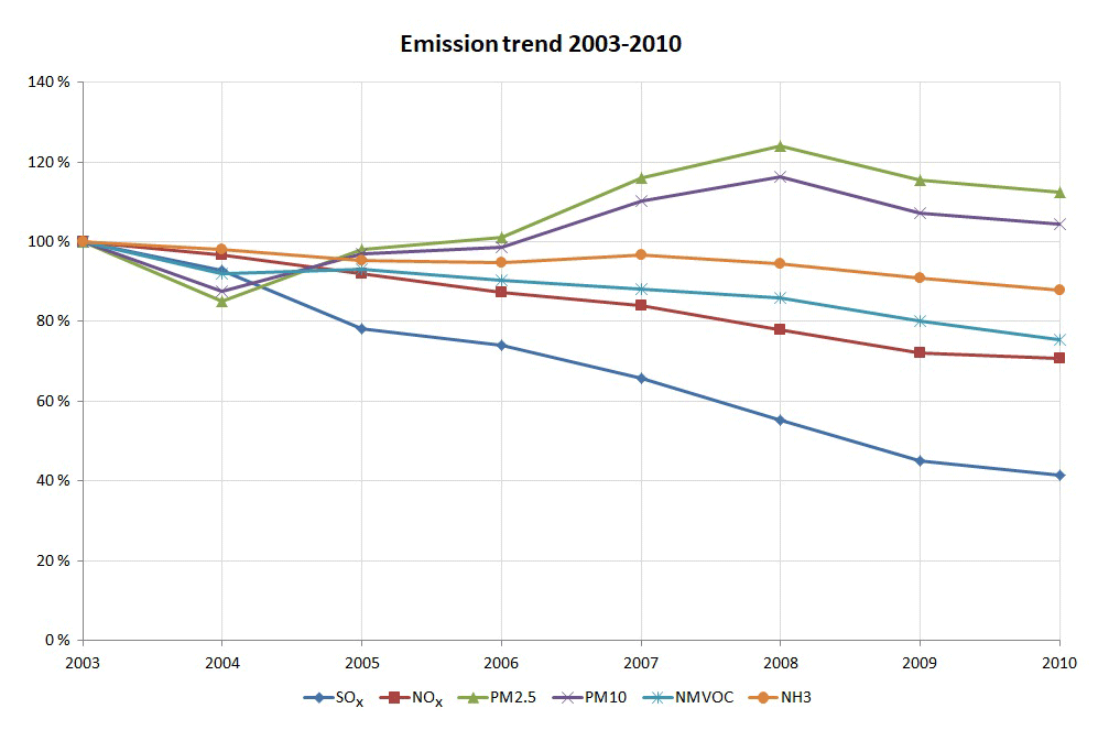
Figure 1Italian anthropogenic emissions, from 2003 to 2010 relative to 2003, elaborated from the ISPRA emission data set described in Taurino et al. (2017).
SOx emissions show the highest reduction, −58 % in the period 2003–2010, followed by NOx (−29 %) due to a large decrease in combustion from energy and road transport sectors, respectively. NMVOC emission reduction is driven by the road transport and solvent use sectors, while NH3 emissions show a very slight decrease. PM2.5 and PM10 emissions increase from 2005 to 2008 due to an increase in biomass combustion in the residential sector (SNAP code 02) (IIR, 2021).
The estimated emissions at the national level need to be further disaggregated in space, before being assigned to the AMS-MINNI grid at 4 km spatial resolution. A provincial distribution (NUTS3 level, where NUTS stands for Nomenclature of Territorial Units for Statistics, the hierarchical system for dividing up the territory of the European Union, https://ec.europa.eu/eurostat/web/nuts/background, last access: 20 January 2020) is provided by ISPRA every 5 years; hence it was available for both the years 2005 and 2010. For the purposes of this work, the 2005 NUTS3 disaggregation was used for the years 2003, 2004, 2005, 2006, and 2007, while the 2010 NUTS3 disaggregation was used for 2008, 2009, and 2010. Finally, hourly and speciated gridded emissions on the AMS-MINNI grid were produced by means of the EMMA processor. The spatial allocation of NUTS3 emissions to the 4 km grid of the MINNI model, for point sources, relied on geographic coordinates of each facility (for example, large combustion plants) and, for diffuse/linear sources, on spatial layers used as proxy variables, like population density (for residential heating and urban traffic), georeferenced road networks (for rural and highway traffic), and land use (for agriculture).
2.4 Meteorological simulations
The meteorological simulations required by AMS-MINNI were elaborated making use of the RAMS model whose main features are summarized in Table 1. The hourly meteorological fields produced by RAMS, such as temperature, wind speed, relative humidity, and precipitation play an important role in determining the level of air pollution concentrations. In trend analysis, it is important to establish the role of the emissions and the meteorology in influencing air pollutant concentration trends. It is out of the scope of the present paper to attribute a relative weight to these factors in determining the analysed concentration trends, but, as a first approximation, we can consider that it could be reasonably attributed to emission trends rather than to a clear tendency in meteorology. In fact, looking at the anomalies (compared to the 1981–2010 climatology) of some meteorological fields for the considered years (2003–2010) computed from NCEP/NCAR reanalyses (National Centers for Environmental Prediction/National Center for Atmospheric Research, Kalnay et al., 1996), it is worth noting that no clear tendency is shown. In Sect. S3 of the Supplement, yearly maps for temperature at 850 hPa (T850), precipitation, and 500 hPa geopotential height (Z500) anomalies are reported, together with the near-surface temperature trend computed from the Copernicus Climate Data Store (CDS, http://climate.copernicus.eu/climate-data-store, last access: 20 January 2020).
2.5 Trend methodology
The detection and calculation of trends in measured and simulated concentrations were performed using the “openair” package (Carslaw and Ropkins, 2012), specifically designed for air pollution data analysis developed for the open source R software (version used: v.3.6.1, http://www.R-project.org, last access: 16 December 2019). The presence of a monotonic increasing or decreasing trend was estimated using the non-parametric Mann–Kendall trend test together with the Theil–Sen method for estimating the slope of a linear trend (as a concentration variation per year) (Mann, 1945; Theil, 1950; Sen, 1968; Kendall, 1975), adopting the deseasonalization option. The calculated trends were regarded as statistically significant if the significance level (i.e. the p value of the Mann–Kendall test) is lower than 0.05 (p < 0.05). This method does not require assumptions about the data distribution, it is not sensitive to outliers, and it has been used in several studies, for example in the EMEP Task Force on Measurements and Modelling during the Eurodelta experiment (Colette et al., 2016) and in the EEA air quality trend reports (EEA, 2009, 2020). Temporal trends were calculated considering monthly averages of the pollutant concentrations at each monitoring stations. Table 2 summarizes the number of stations, grouped per type, with significant and non-significant trends both for observations and modelled estimates.
Table 2Number of stations considered in the trend analysis for the period 2003–2010 separated into background (BKG), traffic (TRA), and industrial (IND) and classified as statistically significant (p < 0.05) for observed, simulated, and both observed and simulated trends.
3.1 Model validation results
Before inspecting the capability of AMS-MINNI to capture the trends of pollutant concentration, a comprehensive evaluation of the model results was carried out.
Comparisons between time series of observed and modelled values were performed on the same set of monitoring stations satisfying the selection criteria used for the trend analysis (i.e. with at least 75 % of valid data per year covering all the 8 years from 2003 to 2010; see Table 2).
For all the pollutants included in the trend analysis, annual time series of daily values were used for the comparison, this metric being considered the most appropriate one for model performances assessment (Colette et al., 2011). For O3, in addition to daily values, the MDA8 metric (maximum daily 8 h average concentration), calculated for the period from April to September, was considered as well, since it turned out to be the most suitable metric for O3 trend analysis within the context of this study (see Sect. 3.2.3).
As recommended by the literature on model validation (Chang and Hanna, 2004), a comprehensive set of statistical indices was computed in order to quantify, from different points of view, the agreement between modelled and observed values.
Here, for the sake of brevity, only three out of all the computed statistical metrics are presented: mean bias (MB), root mean square error (RMSE), and the correlation coefficient (corr); see Sect. S4 in the Supplement for their formulations. These indices were chosen because they capture several features of model performance globally in terms of amplitude, phase, and bias. Moreover, such indicators are frequently used in model evaluation studies (Simon et al., 2012), namely those previously cited on temporal trends. Indeed, in Colette et al. (2011), which we regard as a reference for the present evaluation, model validation is based on the same subset of these three statistical indices. Values of MB, RMSE, and corr for each pollutant are presented here as an average over the 8-year period and over all the available stations, classified according to their type (BKG, TRA, IND) and, for BKG stations, by zone type (rural, suburban, urban).
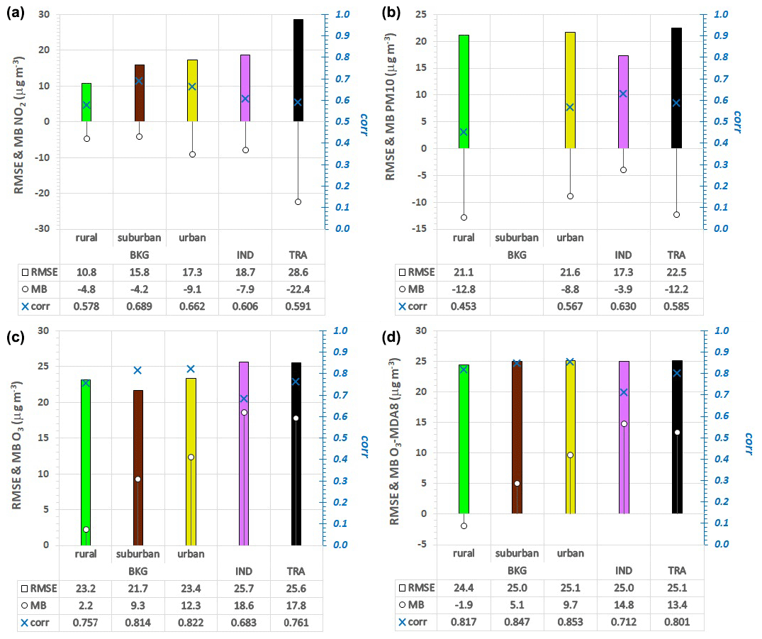
Figure 2Summary of model performance evaluated at all valid Italian monitoring stations during 2003–2010. The statistical scores are based on annual time series of daily average values of NO2 (a), PM10 (b), and O3 (c) and on MDA8 of O3, calculated for the period April–September (d).
Results are shown in Fig. 2 for daily values of NO2 (upper left panel), PM10 (upper right panel), O3 (lower left panel), and for MDA8 of O3 (lower right panel).
Overall, model performance is in line with the results obtained by analogous modelling systems (e.g. Solazzo et al., 2012; Pirovano et al., 2012; Badia and Jorba, 2015; Bessagnet et al., 2016), especially when applied at similar spatial resolution (e.g. Chemel et al., 2010; Pay et al., 2014). More specifically, in Table S2 of Sect. S4 in the Supplement, the statistical score values are reported together with the outcomes of Colette et al. (2011), used hereafter as a reference for an explicit comparison of the performances.
As far as NO2 daily values are concerned (upper left panel of Fig. 2), RMSE and corr values, ranging from 10.8 to 28.6 µg m−3 and from 0.578 to 0.689, respectively, with BKG stations scoring best, are in line with Colette et al. (2011). According to MB, negative values, between −22.4 and −4.2 µg m−3, are obtained for all station types, stressing a general underestimation of NO2 concentration values. Anyway, underestimation is generally lower than in Colette et al. (2011) at BKG stations, getting worse at TRA sites. This feature is commonly expected in chemical transport model applications at a regional scale, and it can be ascribed to the intrinsic difficulties of regional models in capturing, at their resolution, high gradients in spatial concentration variability (Schaap et al., 2015). This hypothesis is confirmed by the evidence that model performance (according to both RMSE and MB) deteriorates with decreasing spatial representativeness of monitoring sites; in particular, absolute values of MB (i.e. underestimations) increase, passing from rural to urban environments and even more at TRA stations.
AMS-MINNI tends to underestimate PM10 daily values too, which is common for regional models, as shown by negative values of MB in the upper right panel of Fig. 2. However, underestimation does not seem to increase with decreasing spatial representativeness of sites and can be attributable to the well-known difficulties of air quality models to take into account all the contributions to PM10 concentration (Solazzo et al., 2012; Im et al., 2015). In particular, it is worth noting that, in the present AMS-MINNI simulations, the contribution of Saharan dust was not included, and this could be the main reason for the underestimation at rural sites. As far as MB and corr are concerned, simulated PM10 concentrations are overall in agreement with observations, with values ranging from −12.8 to −3.9 µg m−3 and from 0.453 to 0.630, respectively.
AMS-MINNI O3 daily values (lower left panel of Fig. 2) are in line with the findings of Colette et al. (2011) concerning both the general overestimation of O3 concentration levels and the range of values of the statistical indices (21.7–25.7 µg m−3 for RMSE, 2.2–18.6 µg m−3 for MB, and 0.683–0.822 for corr). More specifically, Table S2 shows that, for background stations, similar RMSE values are obtained, together with generally lower MB values and better correlation values. Similarly to the performance for NO2, the MB of O3 concentrations changes with the spatial representativeness of monitoring sites, i.e. as NO2 underestimation increases passing from rural to urban environments, O3 overestimation increases, since, close to NO2 sources, the titration process acts as an O3 sink (Seinfeld and Pandis, 1998).
Model performance in reproducing MDA8 of O3 for the period from April to September (lower right panel of Fig. 2) is similar to that for daily concentrations, evaluated throughout the whole year, apart from the negative (albeit small) MB value obtained at rural stations. With respect to daily values, correlation for MDA8 (0.712–0.853) is generally better, as is MB (lower absolute values). With regards to RMSE (24.4–25.1 µg m−3) the values are worse at BKG stations and slightly better at IND and TRA sites. Nevertheless, it is worth noting that, when assessing O3 performance, higher biases in concentration estimates could be expected when using the MDA8 metric, instead of daily average, since concentration levels are higher, too. Indeed, higher MDA8 concentration values are expected when compared with daily values for two reasons: (i) maximum values are taken into account instead of average ones; (ii) only the warm period (April–September) is considered here, when higher O3 values are generally observed.
Globally, AMS-MINNI performs quite well, with the results being in line with the performances of the state of the art of air quality models, when operating at the regional scale and when considering both the values of the statistical indices used for the comparison and the general tendency to overestimate O3 and to underestimate NO2 and PM10.
3.2 Trend analysis
From the concentration fields provided by AMS-MINNI simulations, data were extracted at each monitoring station to compare observed trends (OTs) and simulated trends (STs).
In the following paragraphs, for each of the pollutants considered and for the whole set of stations described in Table 2, an analysis of observed and simulated trends is discussed examining different parameters. For each pollutant, we present
-
the overall distribution of stations with statistically significant and non-significant trends, with their sign, for both observations and simulated values, in order to evaluate model performance in reproducing temporal trends in measured concentrations (Figs. 3, 7, 11);
-
the time series of observed and simulated monthly average concentrations (averaged over all stations for each station type) (Figs. 4a, 5a, 8a, 9a, 12a, 13a);
-
scatter plots of observed and simulated slopes, by station type (Figs. 4b, 5b, 8b, 9b, 12b, 13b);
-
maps of simulated slopes at each grid point, in comparison with the spatial distribution of observed slopes by station type, in order to provide a more detailed description of the results, since observed and simulated slopes are presented according to their spatial distribution and geographical context. Moreover, simulated quantities are provided not only at monitoring sites but at every grid point of the computational domain, to fully exploit model capabilities at their best in terms of both spatial coverage and variability (Figs. 6, 10, 14).
In Sect. S5 of the Supplement the observed and simulated slopes (both in terms of µg m−3 yr−1 and % yr−1) are reported for each pollutant and for each station with a significant trend (p < 0.05).
3.2.1 NO2
Out of 73 monitoring stations, 47(68) have a statistically significant OT (ST), whereas 42 have both significant observed and simulated trends. Figure 3 shows that all STs are negative (93 % significant), whereas 79 % of the OTs were negative (58 % significant; 21 % non-significant) and 21 % were positive (7 % significant; 14 % non-significant). Figures 4a and 5a show that the model reproduces monthly values better at BKG sites than at TRA and IND stations, while the intra-annual variability is well reproduced for all types of stations. This result confirms the good model performance for daily values at BKG stations (Fig. 2).
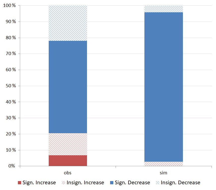
Figure 3Percentage of sites where statistically significant upward trends (dark red), non-significant upward trends (hatched dark red), significant downward trends (dark blue), and non-significant downward trends (hatched dark blue) were obtained for NO2 observations and simulated data.
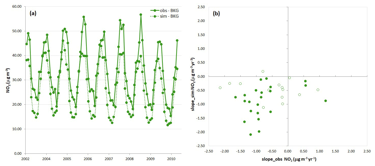
Figure 4(a) Observed (solid line) and simulated (dashed line) monthly means of NO2 concentrations (in µg m−3) for all the background monitoring stations. (b) Scatter plot of observed and simulated slopes (in µg m−3 yr−1) at each individual station. Sites where significant slopes are estimated for both observations and simulated data are indicated with a filled symbol.
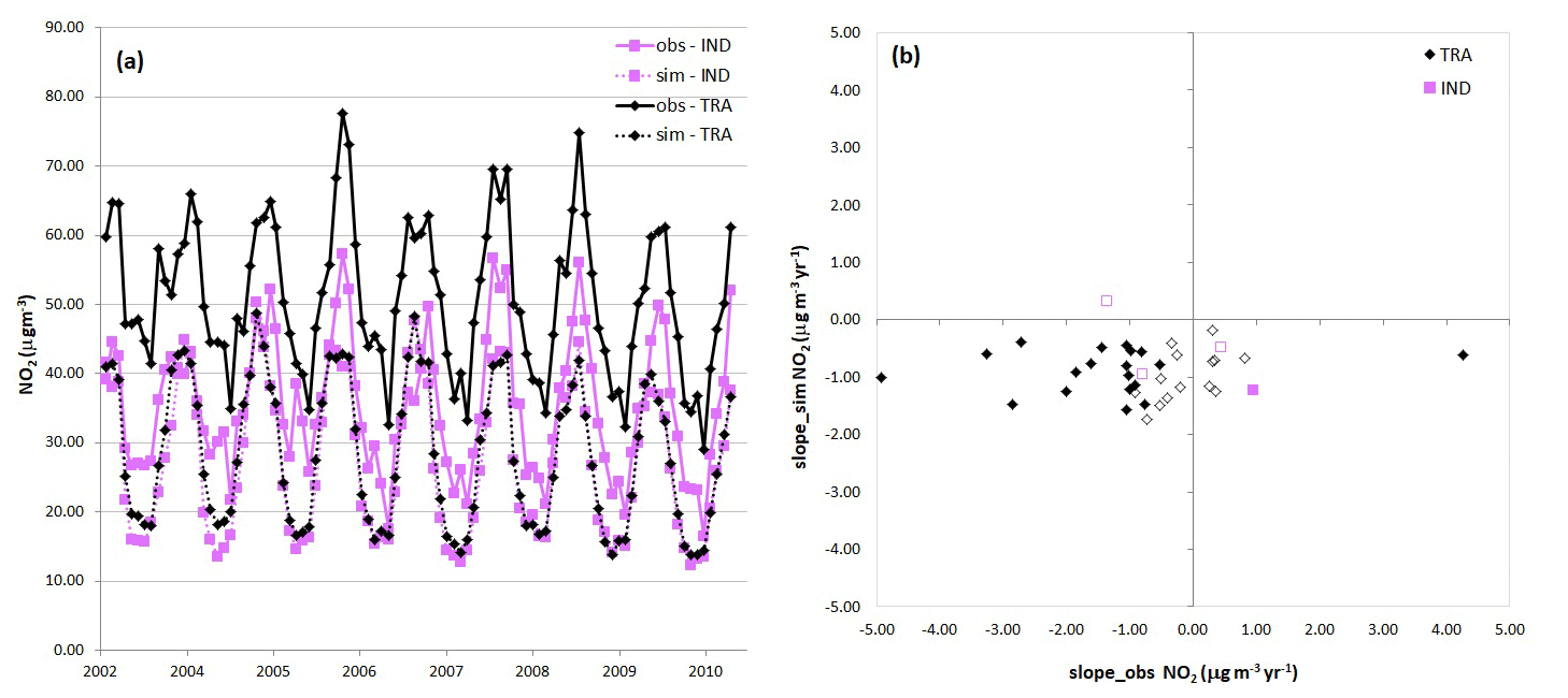
Figure 5(a) Observed (solid line) and simulated (dashed line) monthly means of NO2 concentrations (in µg m−3) for all the traffic (black diamond) and industrial (pink square) monitoring stations. (b) Scatter plot of observed and simulated slopes (in µg m−3 yr−1) at each individual station. Sites where significant slopes are estimated for both observations and simulated data are indicated with a filled symbol.
The scatter plots of Figs. 4b and 5b show an overall good agreement for BKG sites with statistically significant trends, while, as expected, performance is worse at TRA sites where the absolute values of the simulated slopes are mostly lower than the observed ones.
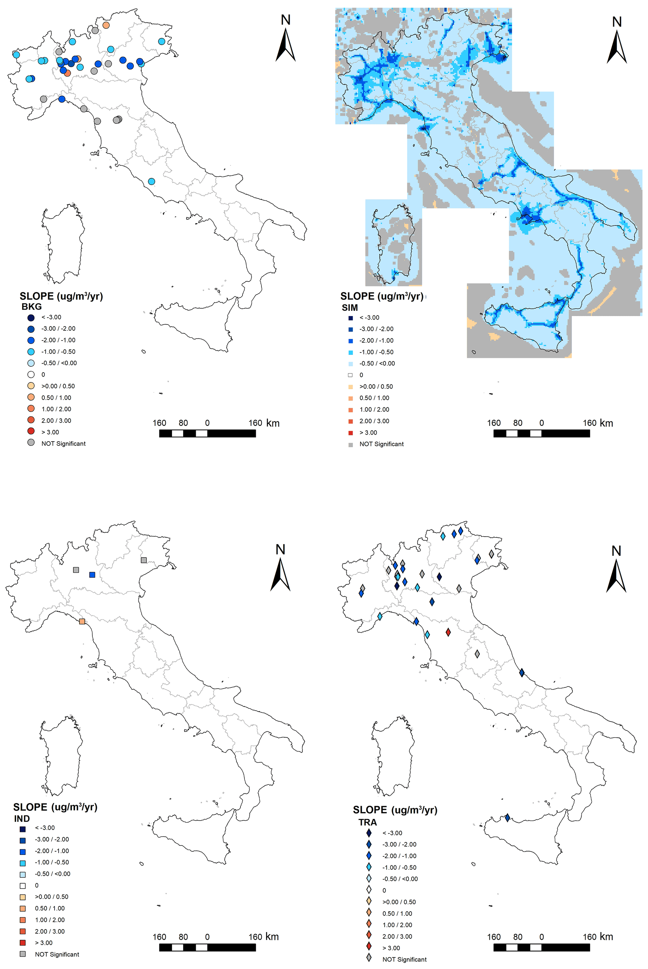
Figure 6Slopes of NO2 (µg m−3 yr−1) observed at background (BKG – upper left panel), industrial (IND – lower left panel), and traffic (TRA – lower right panel) stations and simulated (upper right panel) slopes at each grid point. The grey symbols refer to non-significant trends for both the observations and the simulated data.
Figure 6 shows that model simulations provide coverage and information in parts of the domain where observations are completely absent in the considered period, i.e. in the southern part of Italy. Overall, at BKG stations the model captures both the sign and the variability of the slopes better, while it is worse at TRA stations. The map of the simulated slopes not only has a wider coverage but also shows a greater area with significant trends compared with observations.
3.2.2 PM10
The well-known underestimation of PM10 concentrations when simulated by regional models, already discussed in Sect. 3.1, and the poor quality of the observation network, shown by the low number of stations fulfilling the selection criteria, greatly influenced the trend estimates. Out of 32 monitoring stations, 27(14) have a statistically significant OT (ST), while 11 have both observed and modelled significant trends. The fraction of all the sites with statistically significant observed trends, shown in Fig. 7, is 84 % compared with only 44 % for the ST. The simulated monthly mean time series illustrated in panel a of both Figs. 8 and 9 for BKG and TRA and IND stations, respectively, show a general underestimation of observed concentrations, with performances improving slightly from 2007 onwards. Focussing on sites where both observed and simulated trends are statistically significant, Figs. 8b and 9b show that the model succeeds in capturing not only the sign of all the observed trends but also the slopes at many sites, even if the absolute values are underestimated, especially at the industrial site. This result is confirmed by the maps in Fig. 10, which show a general agreement at most of the available monitoring stations. Although to a lesser extent when compared with NO2 and O3, the simulated statistically significant trends for PM10 cover a wider area with respect to observations especially in the northern area and the island of Sardinia, where no observations are available at all. A poor coverage of significant trends in both model and observations occurs in some areas of central and southern Italy, where the model estimates larger areas of significant trends, especially for the Apulia region and the island of Sicily.
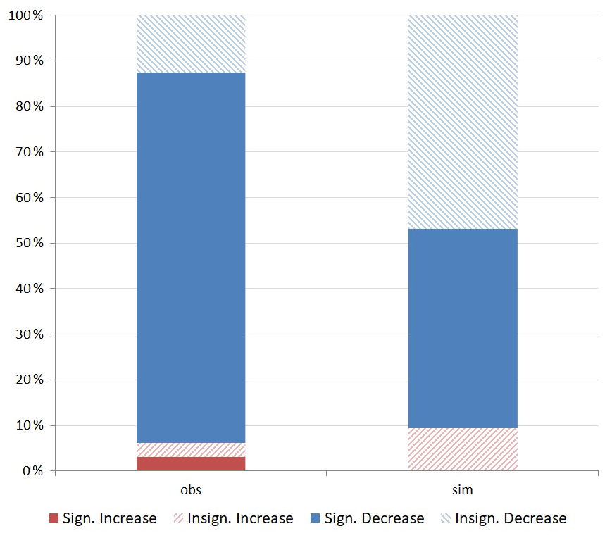
Figure 7Percentage of sites where statistically significant upward trends (dark red), non-significant upward trends (hatched dark red), significant downward trends (dark blue), and non-significant downward trends (hatched dark blue) were obtained for PM10 observations and simulated data.
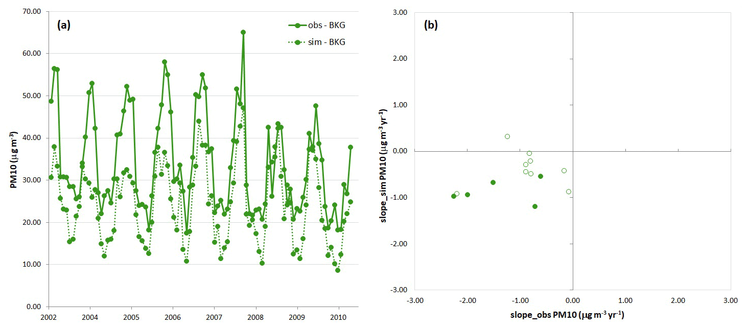
Figure 8(a) Observed (solid line) and simulated (dashed line) monthly means of PM10 concentrations (in µg m−3) for all the background monitoring stations. (b) Scatter plot of observed and simulated slopes (in µg m−3 yr−1) at each individual station. Sites where significant slopes are estimated for both observations and simulated data are indicated with a filled symbol.
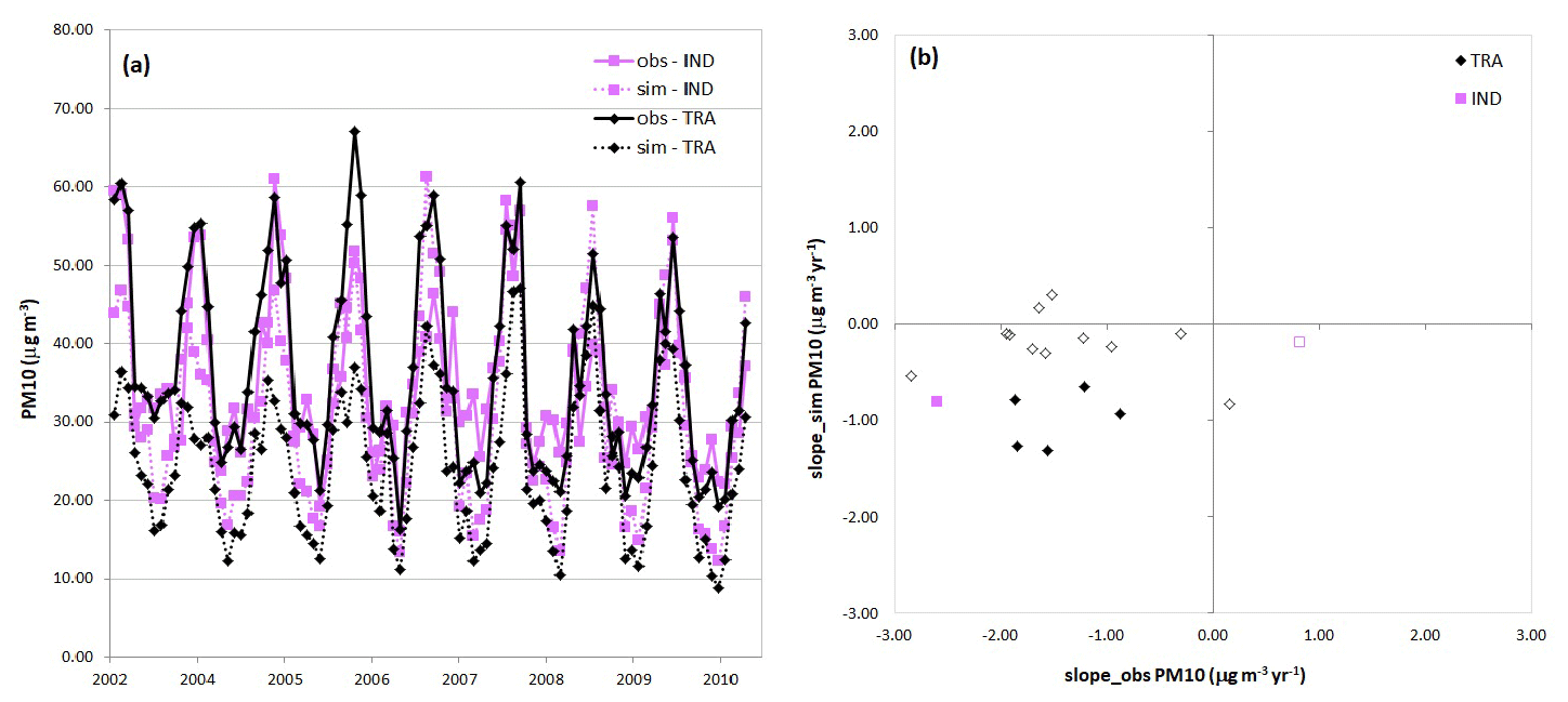
Figure 9(a) Observed (solid line) and simulated (dashed line) monthly means of PM10 concentrations (in µg m−3) for all the traffic (black diamond) and industrial (pink square) monitoring stations. (b) Scatter plot of observed and simulated slopes (in µg m−3 yr−1) at each individual station. Sites where significant slopes are estimated for both observations and simulated data are indicated with a filled symbol.
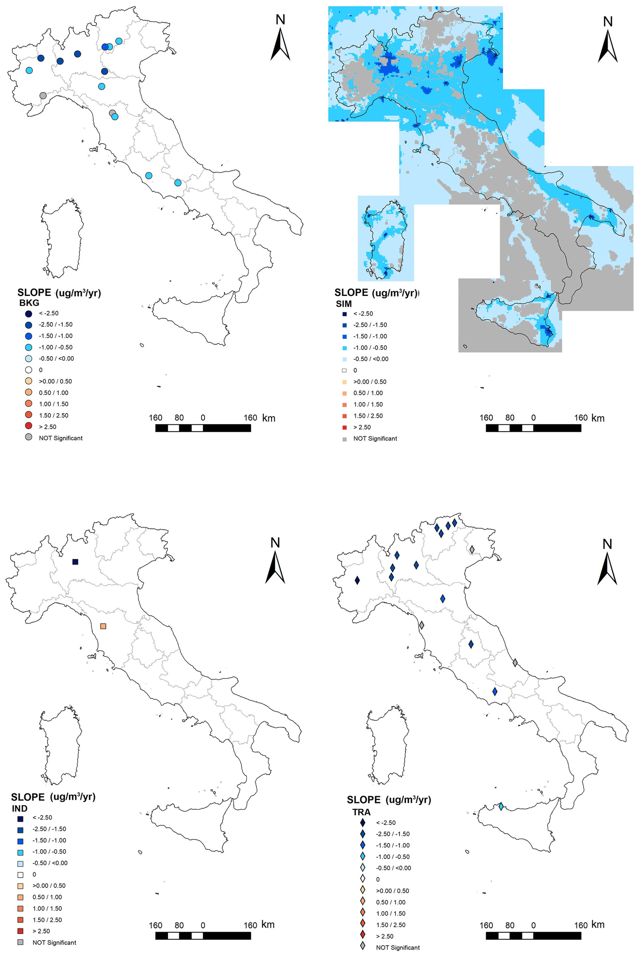
Figure 10Slopes of PM10 (µg m−3 yr−1) observed at background (BKG – upper left panel), industrial (IND – lower left panel), and traffic (TRA – lower right panel) stations and simulated (upper right panel) slopes at each grid point. The grey symbols refer to non-significant trends for both the observations and the simulated data.
3.2.3 O3
As underlined in Lefohn et al. (2017, 2018) and Colette et al. (2017b), the choice of the O3 metrics is of the utmost importance since each indicator could show a different trend. In our analysis, both effect-based indicators (AOT40 and SOMO35) and process-based indicators (MDA8) were computed and analysed. The different metrics explored are the mean O3 concentration (O3 avg); the maximum daily 8 h average concentration (MDA8); the accumulated amount of ozone over the threshold value of 40 ppb (AOT40) calculated from April to September (April–September); and the sum of the daily maxima of the 8 h running average over 35 ppb (SOMO35) for the whole year. Concerning O3 avg and MDA8 metrics, analyses were carried out for both the entire year and from April to September. The number of stations with increasing and decreasing trends and their significance depends on the metric used (Table 2 and Fig. 11). The fraction of stations with significant trends also varies between the observed and modelled data sets. Annual metrics (O3 avg, MDA8, and SOMO35) have a lower fraction of significant trends than the metrics calculated in April–September. For the purpose of our analysis, i.e. to show the capacity of the AMS-MINNI in capturing the air pollution trends through a comparison of observations and simulations, we preferred to focus on the MDA8 indicator calculated in the warm period (April–September), when higher O3 values are generally recorded. Indeed, the MDA8 calculated in the period April–September has the highest number of stations with a significant trend among all indicators.
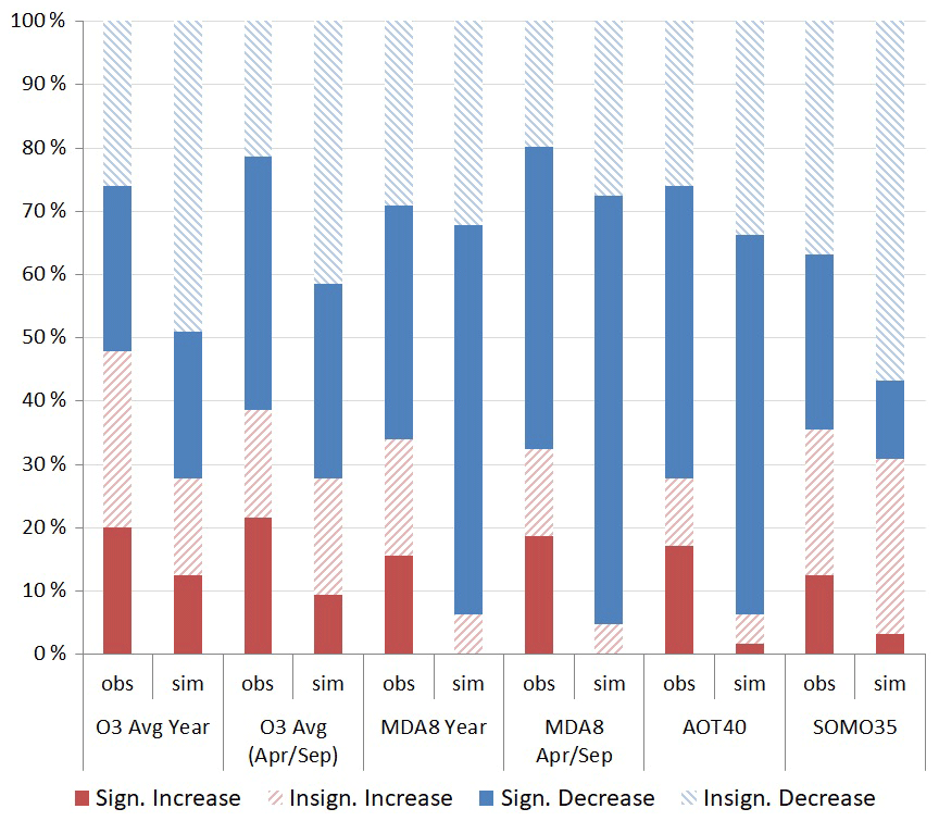
Figure 11Percentage of sites where statistically significant upward trends (dark red), non-significant upward trends (hatched dark red), significant downward trends (dark blue), and non-significant downward trends (hatched dark blue) were obtained for different observed and simulated metrics for O3.

Figure 12(a) Observed (solid line) and simulated (dashed line) monthly means of O3 MDA8 concentrations (in µg m−3) for all the background monitoring stations. (b) Scatter plot of observed and simulated slopes (in µg m−3 yr−1) for O3 MDA8 in the period April–September at each individual station. Sites where significant slopes are estimated for both observations and simulated data are indicated with a filled symbol.
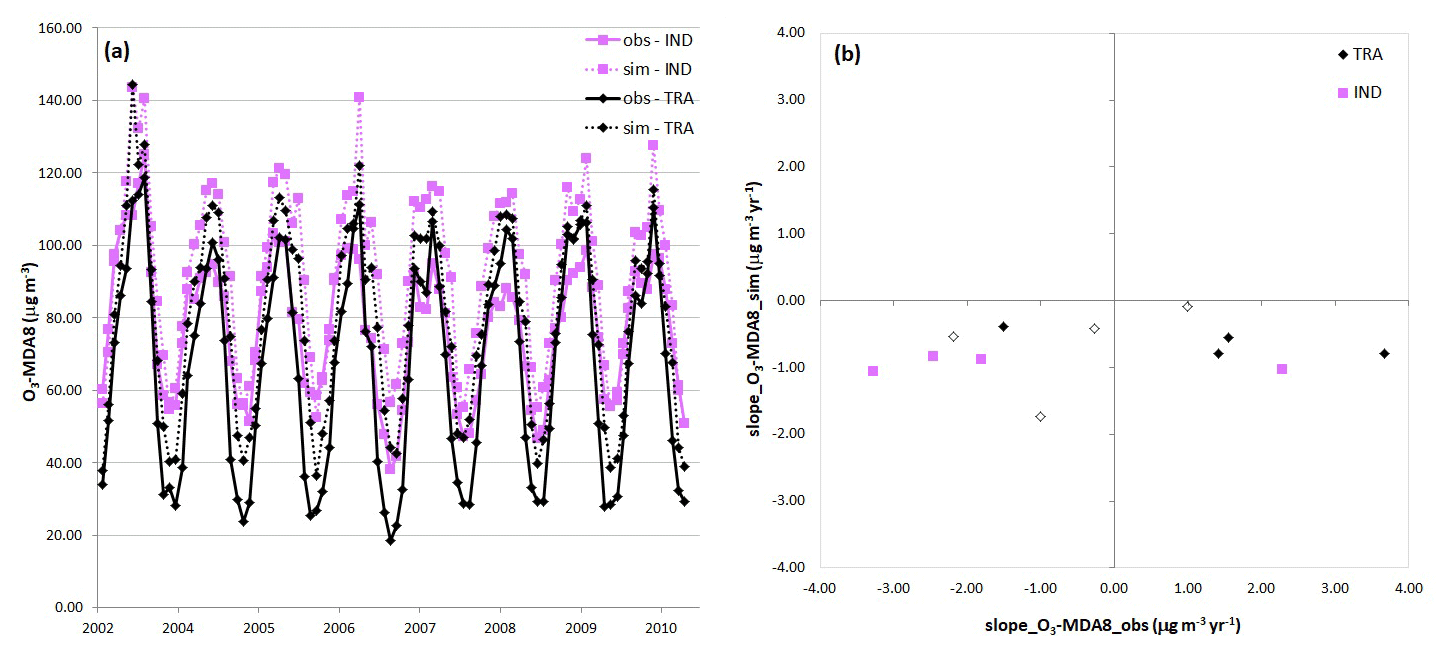
Figure 13(a) Observed (solid line) and simulated (dashed line) monthly means of O3 MDA8 concentrations (in µg m−3) for all the traffic (black diamond) and industrial (pink square) monitoring stations. (b) Scatter plot of observed and simulated slopes (in µg m−3 yr−1) for MDA8 in the period April–September at each individual station. Sites where significant slopes are estimated for both observations and simulated data are indicated with a filled symbol.
The fraction of stations with a significant trend is comparable between observations and simulations (66 % and 68 %, respectively), but when looking at the sign of the trend, we found out that all significant simulated trends are decreasing, while 39 % of significant observed trends are increasing. The monthly mean shows good agreement for BKG stations (Fig. 12a) and a slight overestimation for both IND and TRA stations (Fig. 13a). The scatter plots (panel b of both Figs. 12 and 13) show a higher variability for observed trends than for those simulated.
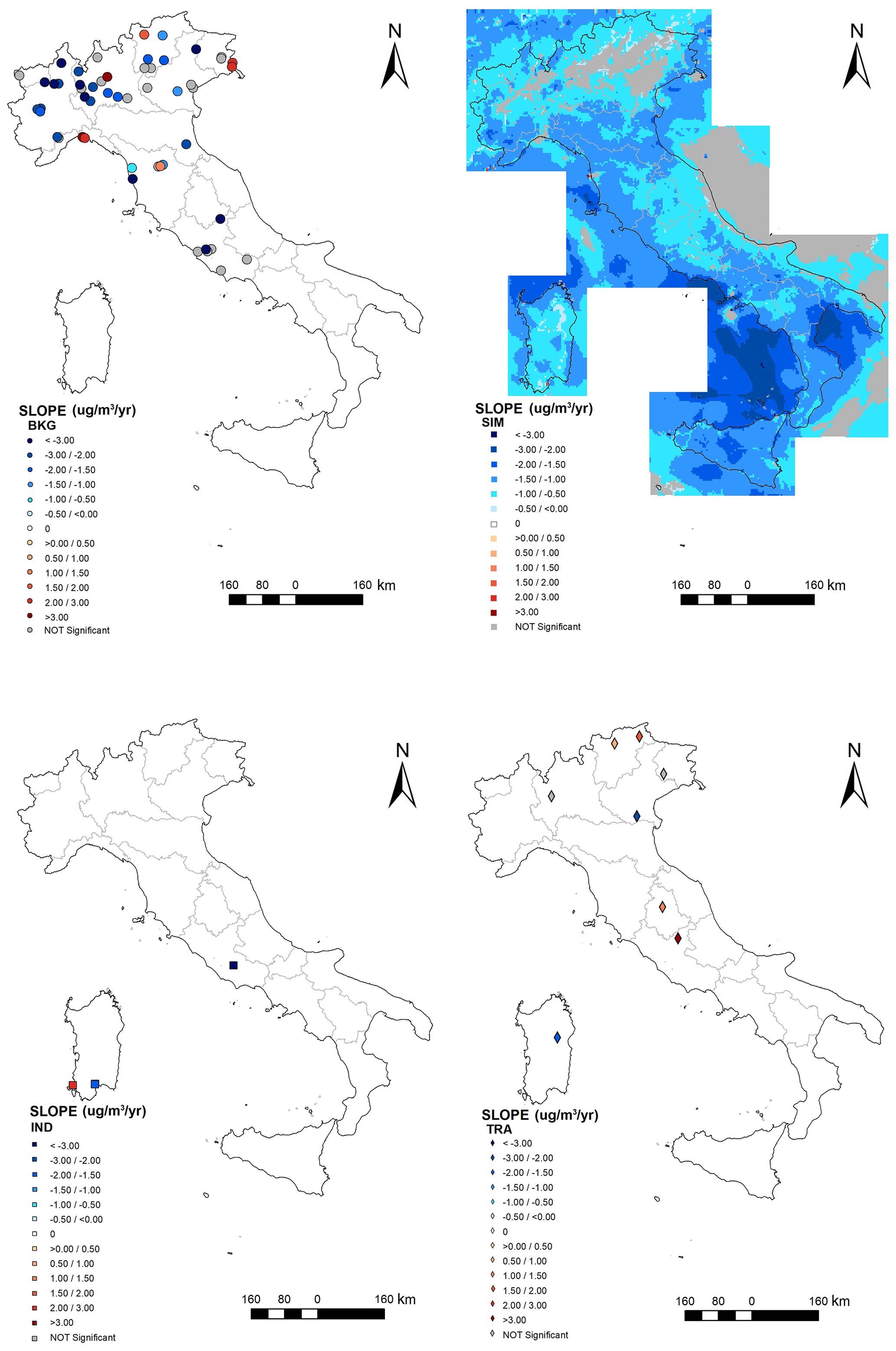
Figure 14Slopes of O3 MDA8 (µg m−3 yr−1) observed at background (BKG – upper left panel), industrial (IND – lower left panel), and traffic (TRA – lower right panel) stations and simulated (upper right panel) slopes at each grid point. The grey symbols refer to non-significant trends for both the observations and the simulated data.
When looking at the spatial distribution, Fig. 14 shows a large area of significant simulated slopes, ranging from −2.0 to −0.5 µg m−3 yr−1 with an area of a non-significant ST in the north-eastern area. The comparison with observations is particularly interesting for BKG stations, for which there are more stations available. As already pointed out, the model does not reproduce the observed positive trends, but the model has good agreement with the significantly decreasing OT, although with a lower variability. Moreover, there are some areas, especially in central and southern Italy, where the model shows a significant trend, whereas monitoring sites are not available at all or the OT is not significant.
3.3 Discussion
Our analysis shows that AMS-MINNI is capable of reproducing observed trends albeit with some differences between the pollutants studied. Although a quantitative analysis of the influence of variations in emissions and meteorology on concentration trends was not performed, we present a preliminary qualitative attempt to compare the temporal concentration trends to variation in emissions, having already observed (see Sect. 2.4) that there is no clear tendency in the meteorology.
The nitrogen oxides (NOx) that are most relevant for air pollution (namely NO and NO2) are mostly emitted during fossil fuel combustion processes and in particular by road transport. In our analysis, the road transport sector represents almost 50 % of all the total emitted NOx (see Fig. S5 of Sect. S2 of the Supplement). The decrease in NO2 concentrations is almost consistent with the decrease in NOx emissions, since NO2 concentrations are directly linked to primary emissions (Colette et al., 2011; Henschel et al., 2015) and mainly driven, in our case, by a reduction in emissions from the road transport sector. Despite the underestimation of absolute values of background concentrations, AMS-MINNI adequately reproduces the observed trends at a national scale (Fig. 4b), demonstrating its potential for supporting reduction policies of background pollution. On the other hand, besides underestimating concentrations at traffic stations like many state-of-the-art CTMs, the decreasing concentration trends observed at traffic stations is underestimated (Fig. 5b). This indicates that the model is either misrepresenting the decrease in emissions or the model is not responding correctly to the changes in emissions. Moreover, the spatial resolution can limit the model's ability to capture large concentration gradients, typical of the urban environment, and this may be the reason for the failure of the model to capture the positive trends. As an interesting example, from Fig. 6 (lower right panel) it turns out that the traffic station with the highest positive observed slope (as shown in Fig. 5b) is located in Florence, Tuscany. The comparison of lower right and upper left panels of Fig. 6 shows that this traffic monitoring site (airbase code IT0861A; see Table S3 of Sect. S5 in the Supplement) is located between two urban BKG sites that have a non-significant OT. The three monitoring points are located within about 4 km (i.e. in the same cell of the computational domain). This is a feature that the model is not able to capture; indeed, in this area simulated trends are not significant or decreasing. Something similar occurs in most of the cases with a positive OT. Most of these points are very close to other monitoring sites where the opposite behaviour (negative slopes) is observed; see for example the couple of BKG sites in Lombardy surrounded by other BKG sites where the opposite sign is found or the IND site located in eastern Liguria very close to a TRA site with a decreasing trend. Therefore, when designing mitigation scenarios at a local urban scale, these results suggest that a regional-scale CTM like AMS-MINNI needs to be integrated with high-resolution models.
Concerning PM and O3, given their secondary nature, a direct link between emissions and atmospheric concentrations is not expected (Guerreiro et al., 2014).
PM10 is both primarily emitted and secondarily generated in the atmosphere from reactions of chemical precursors (NOx, SOx, NH3, NMVOC). Therefore, observed concentrations reflect these and other contributions, like long-range transport, including Saharan dust, in variable fractions depending on the site. The national emissions of primary PM10 (Fig. 1) are stable for the first 4 years (apart from 2004), then grow for 4 years, and diminish in the last period, resulting in a final increase of 13 % from 2003 to 2010. On the other hand, the emissions of all four mentioned precursors decrease at different rates. These contrasting trends in emissions could partly explain the large areas of non-significant trends shown in Fig. 10, whereas the areas with the higher simulated decrease correspond mainly to industrial and traffic areas, underlying the significant efforts in reducing emissions from the industrial and road transport sectors. The few stations available for the comparison show a nice model skill in reproducing observed negative trends, even on TRA stations. This could be a preliminary confirmation of the fitness of AMS-MINNI for the purpose of supporting emission reduction planning, even though further evaluations of model trends are needed, especially for more recent time intervals. Moreover, the observed biases in concentrations, especially at the beginning of the time series (Figs. 8a and 9a), suggest that further insights are needed to investigate how the change in model performances could affect the trend estimates.
O3 is a secondary pollutant produced in the troposphere by the chemical reactions of its precursors, such as NOx and NMVOC, while CH4 and CO become more important at a wider scale (Guerreiro et al., 2014).
The number of cited studies focussing on O3 indicates how critical this pollutant is when exploring relations between temporal trends of emissions and concentrations, given the complex photochemistry, showing sometimes a discrepancy between the emission decrease in O3 precursors and the variation in O3 concentrations (Colette et al., 2011; Guerreiro et al., 2014; Querol et al., 2014). This is particularly important in Mediterranean areas, which are susceptible to ozone-related impacts (De Marco et al., 2019) due to climatological conditions that are more favourable for O3 formation. The national emissions of the main ozone precursors follow a similar descending trend in the 8 years considered; thus there has been little change in the ratio between them, which is the main driver of the chemical equilibrium for O3 formation (Seinfeld and Pandis, 1998; Sillman, 1999). This could partly explain (Fig. 14) why the model gives non-significant trends or trends close to zero in northern Italy, especially in the Po Valley, a well-known air pollution hotspot, densely populated and with high anthropogenic emissions. In the same region where most of the monitoring stations are concentrated, different behaviours of the OT are observed: negative slopes (especially in the western part), non-significant trends, and positive slopes in some stations, mainly located in complex orographic contexts or near the coastline, where the transport of O3 from the sea, caused by sea breeze circulation (Monteiro et al., 2016), together with precursor emission by nearby harbours, could lead to peculiar local features. Similar results can be found in the literature, as for example in Guerreiro et al. (2014) or in Colette et al. (2011), who noticed in particular that different models had different behaviours. On a national level, Cattani et al. (2014) focussed on observations throughout the Italian territory in the period 2003–2012 and showed that it is not possible to estimate a general significant statistical trend (although with a different reference metric, i.e. SOMO0 calculated from April to September), regardless of the type or the area of the stations, and that there are discrepancies in significant trend between adjacent stations. Moreover, as already mentioned, the choice of the O3 metrics can influence the trend estimate. Overall, in our analysis, AMS-MINNI underestimates the absolute value of the descending OT at background stations. This result is driven by north-western monitoring locations, where further work is needed to analyse the quality of local emission estimates and external contributions to ozone concentrations.
The present work aims to assess for the first time the capability of the Italian chemical transport model AMS-MINNI of capturing the trends of three pollutants, namely NO2, PM10, and O3. The analysis for O3 was carried out using different metrics, both for observations and simulations. We firstly conducted a thorough analysis of the model skill considering some statistical score parameters most commonly used in the literature. This analysis confirms that the model performance is in line with the state of the art for regional model applications. Statistical indicators are as good as other CTMs in the literature, and a similar behaviour to that of most regional models was observed concerning the general tendency to overestimate O3 and to underestimate NO2 and PM10. The trend evaluation was performed using the non-parametric Mann–Kendall trend test together with the Theil–Sen method for the estimation of the slopes, and an in-depth comparison between observed and AMS-MINNI modelled trends was carried out. Comparing the sign of modelled and observed trends we found good agreement for almost all sites. Our main result is a general downward simulated trend for the three pollutants. With respect to observations, modelled slopes show the same magnitude for NO2 (in the range −3.0 to −0.5 µg m−3 yr−1), while a smaller variability is detected for PM10 (−1.5 to −0.5 µg m−3 yr−1) and O3 MDA8 (−2.0 to −0.5 µg m−3 yr−1). The reason for the discrepancy for PM10 could be attributed to the well-known underestimation of modelled PM10 concentrations. The results for O3 could be influenced by the poor quality of the monitoring network data in the period we considered, together with the well-documented difficulties of models in capturing O3 concentration trends, given its non-linear dependence on precursor emissions.
Model capabilities in terms of both spatial coverage and variability are illustrated by the maps for the three pollutants, showing a larger area for significant simulated trends compared with those observed, with a larger coverage for NO2 and O3 MDA8 and a smaller one for PM10. For all pollutants, almost the entire domain of northern Italy has significant simulated trends. Even for southern Italy, where in general a low coverage of significant modelled PM10 trends is obtained, there are areas with significant simulated trends where there are no observations. It is also worth noting that in the major islands, Sardinia and Sicily, the simulated trends give useful information, filling the gap due to a sparse or absent monitoring network.
Moreover, a qualitative comparison between the temporal concentration trends and the meteorological and emission variations was carried out, too. Since we do not observe a clear tendency in meteorological anomalies, concentration trends were discussed in connection with emission variations. Indeed, it was pointed out that, due to the complex links between precursor emissions and air pollutant concentrations, emission reductions do not always result in a corresponding decrease in atmospheric concentrations, especially for secondary pollutants like PM10 and O3. Studies on air pollutant trends are relevant to evaluate the impact of the actions taken to reduce emissions in different environmental policies both at national and local levels. The evaluation of the AMS-MINNI capability to reproduce the trends of pollutants increases the reliability of its application in assessing air quality and supporting air quality plans, especially for its use in national regulatory assessments. Indeed, our analysis demonstrates the good agreement between modelled and observed trends and the added value of the model in increasing both the coverage and the significance of air concentration trends with respect to observations. Model performance is best for NO2, while for the others, especially O3, the issue is more challenging. Moreover, the capability to interpret past air quality trends is fundamental in understanding the efficacy of already applied air quality policies and measures and in planning further actions. As demonstrated, the understanding of complex interactions is still uncertain and represents a gap to be filled since it is of the utmost importance in planning future policies aimed at reducing air pollution and its impacts on health and ecosystems.
The present analysis may be applied to other pollutants, especially substances of potential concern for health (e.g. PM2.5). Moreover, it can be considered a reference for other studies in complex geographical conditions such as the Italian territory, which represents an interesting environmental framework, due to its complex orography, resulting in peculiar meteorological conditions, the great variety of natural and anthropogenic contexts, and the presence of the Po Valley, a well-known air pollution hotspot.
| AMS | Atmospheric Modelling System |
| AOT40 | The accumulated amount of ozone over the threshold value of 40 ppb |
| avg | Average |
| BKG | Background |
| BRACE | Banca Dati e Metadati di Qualità dell’aria (National Air Quality database) |
| CDS | Copernicus Climate Data Store |
| CH4 | Methane |
| C6H6 | Benzene |
| CO | Carbon monoxide |
| corr | Correlation coefficient |
| CTM | Chemical transport model |
| EC | European Commission |
| EEA | European Environmental Agency |
| EMAC | ECHAM/MESSy Atmospheric Chemistry |
| EMEP | European Monitoring and Evaluation Programme |
| EMMA | Emission Manager |
| FARM | Flexible Air Quality Regional Model |
| IND | Industrial |
| ISPRA | Istituto Superiore per la Protezione e Ricerca Ambientale (Italian Institute for Environmental Protection and Research) |
| MB | Mean bias |
| MDA8 | Maximum daily 8 h average |
| MINNI | Modello Integrato Nazionale a supporto della Negoziazione Internazionale sui temi dell’Inquinamento atmosferico (Italian National Integrated Model to support the international negotiation on atmospheric pollution) |
| NCEP/NCAR | National Centers for Environmental Prediction/National Center for Atmospheric Research |
| NH3 | Ammonia |
| NMVOCs | Non-methane volatile organic compounds |
| NO | Nitrogen oxide |
| NO2 | Nitrogen dioxide |
| NOx | Nitrogen oxides |
| NUTS | Nomenclature of territorial units for statistics |
| O3 | Ozone |
| obs | Observation |
| OECD | Organization for Economic Co-operation and Development |
| OT | Observed trend |
| PBL | Planetary boundary layer |
| PM2.5 | Particulate matter with a diameter of 2.5 µm or less |
| PM10 | Particulate matter with a diameter of 10 µm or less |
| RAMS | Regional Atmospheric Modelling System |
| RMSE | Root mean square error |
| SIA | Secondary inorganic aerosol |
| sim | Simulation |
| SNAP | Selective Nomenclature for Air Pollution |
| SOx | Sulfur dioxide |
| SOA | Secondary organic aerosol |
| SOMO35 | Sum of the daily maxima of the 8 h running average over 35 ppb |
| ST | Simulated trend |
| SURFPRO | SURFace-atmosphere interface PROcessor |
| T850 | Temperature at 850 hPa |
| TKE | Turbulent kinetic energy |
| TRA | Traffic |
| UNECE | United Nations Economic Commission for Europe |
| WHO | World Health Organization |
| Z500 | 500 hPa geopotential height |
The meteorological model RAMS v6.0 is freely available at http://www.atmet.com/software/rams_soft.shtml (Cotton et al., 2003). The chemical transport model FARM v4.7.0 is freely available upon request to ARIANET s.r.l. (http://www.aria-net.it, last access: 14 July 2021). The emission software emma6 is available on charge upon request to ARIANET s.r.l. All the codes can be provided confidentially for the editor and reviewers in order to enable peer review. All the modelled data (gridded emissions, meteorological and concentration fields at 4 km resolution) and the trend analysis calculations are available upon request to the authors. Observation data are publicly available from the BRACE website (http://www.brace.sinanet.apat.it/web/struttura.html?p_livello_1=18&p_main=web/area_download.inizio&p_scroll=, ISPRA, 2021).
The supplement related to this article is available online at: https://doi.org/10.5194/acp-21-10825-2021-supplement.
ID'E, LV, GR, and AP put original effort into conceptualization, methodology, and study and interpretation of the trend analysis. MD'I, GB, and AC performed the model simulations; ID'E and GB carried out the data processing; ID'E, LV, GR, AP, and MD'I wrote the original draft, including visualization, and performed the review and editing; AC, GB, MA, MM, GZ, and LC contributed to the writing review and editing; GZ and LC accomplished the acquisition of funds.
The authors declare that they have no conflict of interest.
Publisher’s note: Copernicus Publications remains neutral with regard to jurisdictional claims in published maps and institutional affiliations.
The computing resources and the related technical support used for the AMS-MINNI simulations were provided by the CRESCO/ENEAGRID High Performance Computing infrastructure and its staff (Iannone et al., 2019). The infrastructure is funded by ENEA, the Italian National Agency for New Technologies, Energy and Sustainable Economic Development and by Italian and European research programmes (http://www.cresco.enea.it/english, last access: 14 July 2021). We would like to express our thanks to Giorgio Cattani (ISPRA) for the support in gathering observation data. We also thank the three anonymous reviewers for their accurate and very useful comments.
Part of the simulations of this research has been supported by ENEL under the contract agreement no. 1400519908 between ENEA and ENEL. The article processing charge has been funded by the Italian Ministry for the Ecological Transition under the contract agreement no. I36C18006110001 between ENEA and the Italian Ministry for the Ecological Transition.
This paper was edited by Veli-Matti Kerminen and reviewed by three anonymous referees.
Airbase: Air quality e-reporting, available at: https://www.eea.europa.eu/data-and-maps/data/aqereporting-8, last access: 15 July 2020.
Amato, F., Karanasiou, A., Moreno, T., Alastuey, A., Orza, J., Lumbreras, J., Borge, R., Boldo, E., Linares, C., and Querol, X.: Emission factors from road dust resuspension in a Mediterranean freeway, Atmos. Environ., 61, 580–587, https://doi.org/10.1016/j.atmosenv.2012.07.065, 2012.
Apte, J. S., Brauer, M., Cohen, A. J., Ezzati, M., and Pope III, C. A.: Ambient PM2.5 Reduces Global and Regional Life Expectancy, Environ. Sci. Tech. Lett., 5, 546–551, https://doi.org/10.1021/acs.estlett.8b00360, 2018.
Arianet: SURFPRO3 User's guide (SURFace-atmosphere interface PROcessor, Version 3), Software manual, Arianet R2011.31, Milan, Italy, 2011.
Arianet: Emission Manager. Modular processing system for model-ready emission input Preparation, Software Manual, Milan, Italy, 2014.
Badia, A. and Jorba, O.: Gas-phase evaluation of the online NMMB/BSC-CTM model over Europe for 2010 in the framework of the AQMEII-Phase2 project, Atmos. Environ., 115, 657–669, https://doi.org/10.1016/j.atmosenv.2014.05.055, 2015.
Bessagnet, B., Pirovano, G., Mircea, M., Cuvelier, C., Aulinger, A., Calori, G., Ciarelli, G., Manders, A., Stern, R., Tsyro, S., García Vivanco, M., Thunis, P., Pay, M.-T., Colette, A., Couvidat, F., Meleux, F., Rouïl, L., Ung, A., Aksoyoglu, S., Baldasano, J. M., Bieser, J., Briganti, G., Cappelletti, A., D'Isidoro, M., Finardi, S., Kranenburg, R., Silibello, C., Carnevale, C., Aas, W., Dupont, J.-C., Fagerli, H., Gonzalez, L., Menut, L., Prévôt, A. S. H., Roberts, P., and White, L.: Presentation of the EURODELTA III intercomparison exercise – evaluation of the chemistry transport models' performance on criteria pollutants and joint analysis with meteorology, Atmos. Chem. Phys., 16, 12667–12701, https://doi.org/10.5194/acp-16-12667-2016, 2016.
Bigi, A. and Ghermandi, G.: Trends and variability of atmospheric PM2.5 and PM10–2.5 concentration in the Po Valley, Italy, Atmos. Chem. Phys., 16, 15777–15788, https://doi.org/10.5194/acp-16-15777-2016, 2016.
Binkowski, F. S. and Roselle, S. J.: Models-3 community multiscale air quality (CMAQ) model aerosol component 1. Model description, J. Geophys. Res., 108, 4183, https://doi.org/10.1029/2001JD001409, 2003.
BRACE: http://www.brace.sinanet.apat.it/web/struttura.html (last access: 14 July 2021), 2013.
Cadum, E., Rossi, G., Mirabelli, D., Vigotti, M.A., Natale, P., Albano, L., Marchi, G., Di Meo, V., Cristofani, R., and Costa, G.: Air pollution and daily mortality in Turin, 1991–1996, Epidemiologia e Prevenzione, 23, 268–276, available at: https://europepmc.org/article/med/10730467 (last access: 15 May 2020), 1999 (in Italian).
Carnell, E., Vieno, M., Vardoulakis, S., Beck, R., Heaviside, C., Tomlinson, S., Dragosits, U., Healand, M. R., and Reis, S.: Modelling public health improvements as a result of air pollution control policies in the UK over four decades – 1970 to 2010, Environ. Res. Lett., 14, 074001, https://doi.org/10.1088/1748-9326/ab1542, 2019.
Carslaw, D. C. and Ropkins, K.: Openair – an R package for air quality data analysis, Environ. Modell. Softw., 27–28, 52–61, https://doi.org/10.1016/j.envsoft.2011.09.008, 2012.
Carter, W. P. L.: Documentation of the SAPRC-99 chemical mechanism for VOC reactivity assessment. Final Report to California Air Resources Board, Contract No. 92-329, and (in part) 95-308, Sacramento, CA, USA, 2000.
Carugno, M., Consonni, D., Bertazzi, P.A., Biggeri, A., and Baccini, M.: Temporal trends of PM10 and its impact on mortality in Lombardy, Italy, Environ. Poll., 227, 280–286, https://doi.org/10.1016/j.envpol.2017.04.077, 2017.
Casale, G. R., Meloni, D., Miano, S., Palmieri, S., Siani, A. M., and Cappellani, F.: Solar UV-B irradiance and total ozone in Italy: Fluctuations and trends, J. Geophys. Res., 105, 4895-4901, https://doi.org/10.1029/1999JD900303, 2000.
Cattani, G., Di Menno di Bucchianico, A., Dina, D., Inglessis, M., Notaro, C., Settimo, G., Viviano, G., and Marconi, A.: Evaluation of the temporal variation of air quality in Rome, Italy, from 1999 to 2008, Ann. Ist. Super Sanità, 46, 242–253, https://doi.org/10.4415/ANN_10_03_04, 2010.
Cattani, G., Bernetti, A., Caricchia, A., De Lauretis, R., De Marco, S., Di Menno di Bucchianico, A., Gaeta, A., Gandolfo, G., and Taurino, E.: Analisi dei trend dei principali inquinanti atmosferici in Italia 2003–2012, ISPRA, Rome, Italy, report 203/2014, 2014 (in Italian).
Cattani, G., Di Menno di Bucchianico, A., Fioravanti, G., Gaeta, A., Gandolfo, G., Lena, F., and Leone, G.: Analisi dei trend dei principali inquinanti atmosferici in Italia 2008–2017, ISPRA, Rome, Italy, report 302/2018, 2018 (in Italian).
Chang, J. C. and Hanna, S. R.: Air quality model performance evaluation, Meteorol. Atmos. Phys., 87, 167–196, https://doi.org/10.1007/s00703-003-0070-7, 2004.
Chemel, C., Sokhi, R. S., Yu, Y., Hayman, G. D., Vincent, K. J., Dore, A. J., Tang, Y. S., Prain, H. D., and Fisher, B.: Evaluation of a CMAQ simulation at high resolution over the UK for the calendar year 2003, Atmos. Environ., 44, 2927–2939, https://doi.org/10.1016/j.atmosenv.2010.03.029, 2010.
Chen, C. and Cotton, W. R.: A one-dimensional simulation of the stratocumulus-capped mixed layer, Bound.-Lay. Meteorol., 25, 289–321, https://doi.org/10.1007/BF00119541, 1983.
Ciarelli, G., Theobald, M. R., Vivanco, M. G., Beekmann, M., Aas, W., Andersson, C., Bergström, R., Manders-Groot, A., Couvidat, F., Mircea, M., Tsyro, S., Fagerli, H., Mar, K., Raffort, V., Roustan, Y., Pay, M.-T., Schaap, M., Kranenburg, R., Adani, M., Briganti, G., Cappelletti, A., D'Isidoro, M., Cuvelier, C., Cholakian, A., Bessagnet, B., Wind, P., and Colette, A.: Trends of inorganic and organic aerosols and precursor gases in Europe: insights from the EURODELTA multi-model experiment over the 1990–2010 period, Geosci. Model Dev., 12, 4923–4954, https://doi.org/10.5194/gmd-12-4923-2019, 2019.
Ciucci, A., D'Elia, I., Wagner, F., Sander, R., Ciancarella, L., Zanini, G., and Schöpp, W.: Cost-effective reductions of PM2.5 concentrations and exposure in Italy, Atmos. Environ., 140, 84–93, https://doi.org/10.1016/j.atmosenv.2016.05.049, 2016.
Cohen, A. J., Brauer, M., Burnett, R., Anderson, H. R., Frostad, J., Estep, K., Balakrishnan, K., Brunekreef, B., Dandona, L., Dandona, R., Feigin, V., Freedman, G., Hubbell, B., Jobling, A., Kan, H., Knibbs, L., Liu, Y., Martin, R., Morawska, L., Pope, C. A., Shin, H., Straif, K., Shaddick, G., Thomas, M., van Dingenen, R., van Donkelaar, A., Vos, T., Murray, C. J. L., and Forouzanfar, M. H.: Estimates and 25-year trends of the global burden of disease attributable to ambient air pollution: an analysis of data from the Global Burden of Diseases Study 2015, Lancet, 389, 1907–1918, https://doi.org/10.1016/S0140-6736(17)30505-6, 2017.
Colette, A., Granier, C., Hodnebrog, Ø., Jakobs, H., Maurizi, A., Nyiri, A., Bessagnet, B., D'Angiola, A., D'Isidoro, M., Gauss, M., Meleux, F., Memmesheimer, M., Mieville, A., Rouïl, L., Russo, F., Solberg, S., Stordal, F., and Tampieri, F.: Air quality trends in Europe over the past decade: a first multi-model assessment, Atmos. Chem. Phys., 11, 11657–11678, https://doi.org/10.5194/acp-11-11657-2011, 2011.
Colette, A., Aas, W., Banin, L., Braban, C. F., Ferm, M., González Ortiz, A., Ilyin, I., Mar, K., Pandolfi, M., Putaud, J.-P., Shatalov, V., Solberg, S., Spindler, G., Tarasova, O., Vana, M., Adani, M., Almodovar, P., Berton, E., Bessagnet, B., Bohlin-Nizzetto, P., Boruvkova, J., Breivik, K., Briganti, G., Cappelletti, A., Cuvelier, K., Derwent, R., D'Isidoro, M., Fagerli, H., Funk, C., Garcia Vivanco, M., Haeuber, R., Hueglin, C., Jenkins, S., Kerr, J., de Leeuw, F., Lynch, J., Manders, A., Mircea, M., Pay, M. T., Pritula, D., Querol, X., Raffort, V., Reiss, I., Roustan, Y., Sauvage, S., Scavo, K., Simpson, D., Smith, R. I., Tang, Y. S., Theobald, M., Tørseth, K., Tsyro, S., van Pul, A., Vidic, S., Wallasch, M., and Wind, P.: Air pollution trends in the EMEP region between 1990 and 2012, NILU, Oslo, Norway, 2016.
Colette, A., Andersson, C., Manders, A., Mar, K., Mircea, M., Pay, M.-T., Raffort, V., Tsyro, S., Cuvelier, C., Adani, M., Bessagnet, B., Bergström, R., Briganti, G., Butler, T., Cappelletti, A., Couvidat, F., D'Isidoro, M., Doumbia, T., Fagerli, H., Granier, C., Heyes, C., Klimont, Z., Ojha, N., Otero, N., Schaap, M., Sindelarova, K., Stegehuis, A. I., Roustan, Y., Vautard, R., van Meijgaard, E., Vivanco, M. G., and Wind, P.: EURODELTA-Trends, a multi-model experiment of air quality hindcast in Europe over 1990–2010, Geosci. Model Dev., 10, 3255–3276, https://doi.org/10.5194/gmd-10-3255-2017, 2017a.
Colette, A., Solberg, S., Beauchamp, M., Bessagnet, B., Malherbe, L., Guerreiro, C., Andersson, A., Cuvelier, C., Manders, A., Mar, K. A., Mircea, M., Pay, M. T., Raffort, V., Tsyro, S., Adani, M., Bergström, R., Briganti, G., Cappelletti, A., Couvidat, F., D'Isidoro, M., Fagerli, H., Ojha, N., Otero, N., and Wind, P.: Long term air quality trends in Europe. Contribution of meteorological variability, natural factors and emissions, ETC/ACM, Bilthoven, the Netherlands, Technical Paper 2016/7, 2017b.
Cotton, W. R., Pielke Sr., R. A., Walko, R. L., Liston, G. E., Tremback, C. J., Jiang, H., McAnelly, R. L., Harrington, J. Y., Nicholls, M. E., Carrio, G. G., and McFadden, J. P.: RAMS 2001: Current status and future directions, Meteorol. Atmos. Phys., 82, 5–29, https://doi.org/10.1007/s00703-001-0584-9, 2003 (data available at: http://www.atmet.com/software/rams_soft.shtml, last access: 19 October 2020).
Cristofanelli, P., Scheel, H.-E., Steinbacher, M., Saliba, M., Azzopardi, F., Ellul, R., Fröhlich, M., Tositti, L., Brattich, E., Maione, M., Calzolari, F., Duchi, R., Landi, T. C., Marinoni, A., and Bonasoni, P.: Long-term surface ozone variability at Mt. Cimone WMO/GAW global station (2165 m a.s.l., Italy), Atmos. Environ., 101, 23–33, https://doi.org/10.1016/j.atmosenv.2014.11.012, 2015.
D'Elia, I., Bencardino, M., Ciancarella, L., Contaldi, M., and Vialetto, G.: Technical and Non-Technical Measures for air pollution emission reduction: The integrated assessment of the regional Air Quality Management Plans through the Italian national model, Atmos. Environ., 43, 6182–6189, https://doi.org/10.1016/j.atmosenv.2009.09.003, 2009.
D'Elia, I., Piersanti, A., Briganti, G., Cappelletti, A., Ciancarella, L., and Peschi, E.: Evaluation of mitigation measures for air quality in Italy in 2020 and 2030, Atmos. Poll. Res., 9, 977–988, https://doi.org/10.1016/j.apr.2018.03.002, 2018.
De Marco, A., Proietti, C., Anav, A., Ciancarella, L., D'Elia, I., Fares, S., Fornasier, M.F., Fusaro, L., Gualtieri, M., Manes, F., Marchetto, A., Mircea, M., Paoletti, E., Piersanti, A., Rogora, M., Salvati, L., Salvatori, E., Screpanti, A., and Leonardi, C.: Impacts of air pollution on human and ecosystem health, and implications for the National Emission Ceilings Directive: Insight from Italy, Environ. Int., 125, 320–333, https://doi.org/10.1016/j.envint.2019.01.064, 2019.
Dufour, G., Eremenko, M., Beekmann, M., Cuesta, J., Foret, G., Fortems-Cheiney, A., Lachâtre, M., Lin, W., Liu, Y., Xu, X., and Zhang, Y.: Lower tropospheric ozone over the North China Plain: variability and trends revealed by IASI satellite observations for 2008–2016, Atmos. Chem. Phys., 18, 16439–16459, https://doi.org/10.5194/acp-18-16439-2018, 2018.
European Commission (EC): Council Decision 97/101/EC of 27 January 1997 establishing a reciprocal exchange of information and data from networks and individual stations measuring ambient air pollution within the Member States, Official Journal of the European Communities, L 35, 14–22, 1997.
European Commission (EC): Directive 2008/50/EC of the European Parliament and of the Council of 21 May 2008 on ambient air quality and cleaner air for Europe (The Framework Directive), Official Journal European Union En. Series, OJ L 152, 11 June 2008, 1–44, Brussels, Belgium, 2008.
European Commission (EC): Directive (EU) 2016/2284 of the European Parliament and of the Council of 14 December 2016 on the reduction of national emissions of certain atmospheric pollutants, amending Directive 2003/35/EC and repealing Directive 2001/81/EC. Official Journal of the European Union, OJ L 344, 17 December 2016, 1–31, Brussels, Belgium, 2016.
European Environmental Agency (EEA): Assessment of ground-level ozone in EEA member countries, with a focus on long-term trends, European Environment Agency, Copenhagen, Denmark, 56, https://doi.org/10.2800/11798, 2009.
European Environmental Agency (EEA): Air quality in Europe – 2020 report. EEA, Luxembourg: Publications Office of the European Union, Luxembourg Report, 09/2020, https://doi.org/10.2800/786656, 2020.
Feng, Z., De Marco, A., Anav, A., Gualtieri, M., Sicard, P., Tian, H., Fornasier, F., Tao, F., Guo, A., and Paoletti, E.: Economic losses due to ozone impacts on human health, forest productivity and crop yield across China, Environ. Int., 131, 104966, https://doi.org/10.1016/j.envint.2019.104966, 2019.
Fountoukis, C. and Nenes, A.: ISORROPIA II: a computationally efficient thermodynamic equilibrium model for K+–Ca2+–Mg2+––Na+–––Cl−–H2O aerosols, Atmos. Chem. Phys., 7, 4639–4659, https://doi.org/10.5194/acp-7-4639-2007, 2007.
Fuzzi, S., Baltensperger, U., Carslaw, K., Decesari, S., Denier van der Gon, H., Facchini, M. C., Fowler, D., Koren, I., Langford, B., Lohmann, U., Nemitz, E., Pandis, S., Riipinen, I., Rudich, Y., Schaap, M., Slowik, J. G., Spracklen, D. V., Vignati, E., Wild, M., Williams, M., and Gilardoni, S.: Particulate matter, air quality and climate: lessons learned and future needs, Atmos. Chem. Phys., 15, 8217–8299, https://doi.org/10.5194/acp-15-8217-2015, 2015.
Gariazzo, C., Silibello, C., Finardi, S., Radice, P., Piersanti, A., Calori, G., Cecinato, A., Perrino, C., Nussio, F., Cagnoli, M., Pelliccioni, A., Gobbi, G. P., and Di Filippo, P.: A gas/aerosol air pollutants study over the urban area of Rome using a comprehensive chemical transport model, Atmos. Environ., 41, 7286–7303, https://doi.org/10.1016/j.atmosenv.2007.05.018, 2007.
Gilardoni, S., Tarozzi, L., Sandrini, S., Ielpo, P., Contini, D., Putaud, J-P., Cavalli, F., Poluzzi, V., Bacco, D., Leonardi, C., Genga, A., Langone, L., and Fuzzi, S.: Reconstructing Elemental Carbon Long-Term Trend in the Po Valley (Italy) from Fog Water Samples, Atmos., 11, 580, https://doi.org/10.3390/atmos11060580, 2020.
Gualtieri, G., Crisci, A., Tartaglia, M., Toscano, P., Vagnoli, C., Adreini, B. P., and Gioli, B.: Analysis of 20-year air quality trends and relationship with emission data: The case of Florence (Italy), Urban Climate, 10, 530–549, https://doi.org/10.1016/j.uclim.2014.03.010, 2014.
Guenther, A., Karl, T., Harley, P., Wiedinmyer, C., Palmer, P. I., and Geron, C.: Estimates of global terrestrial isoprene emissions using MEGAN (Model of Emissions of Gases and Aerosols from Nature), Atmos. Chem. Phys., 6, 3181–3210, https://doi.org/10.5194/acp-6-3181-2006, 2006.
Guerreiro, C. B. B., Foltescu, V., and de Leeuw, F.: Air quality status and trends in Europe, Atmos. Environ., 98, 376–384, https://doi.org/10.1016/j.atmosenv.2014.09.017, 2014.
Henschel, S., Le Tertre, A., Atkinson, R. W., Querol, X., Pandolfi, M., Zeka, A., Haluza, D., Analitis, A., Katsouyanni, K., Bouland, C., Pascal, M., Medina, S., and Goodman, P. G.: Trends of nitrogen oxides in ambient air in nine European cities between 1999 and 2010, Atmos. Environ., 117, 234–241, https://doi.org/10.1016/j.atmosenv.2015.07.013, 2015.
Iannone, F., Ambrosino, F., Bracco, G., De Rosa, M., Funel, A., Guarnieri, G., Migliori, S., Palombi, F., Ponti, G., Santomauro, G., and Procacci, P.: CRESCO ENEA HPC clusters: a working example of a multifabric GPFS Spectrum Scale layout, 2019 International Conference on High Performance Computing & Simulation (HPCS), 15–19 July 2019, Dublin, Ireland, 1051–1052, https://doi.org/10.1109/HPCS48598.2019.9188135, 2019.
IIR: Italian Emission Inventory 1990–2019, Informative Inventory Report 2021. Ispra Technical Report, 342/2021, Rome, Italy, 2021.
Im, U., Bianconi, R., Solazzo, E., Kioutsioukis, I., Badia, A., Balzarini, A., Baró, R., Bellasio, R., Brunner, D., Chemel, C., Curci, G., van der Gon, H. D., Flemming, J., Forkel, R., Giordano, L., Jiménez-Guerrero, P., Hirtl, M., Hodzic, A., Honzak, L., Jorba, O., Knote, C., Makar, P.A., Manders-Groot, A., Neal, L., Pérez, J. L., Pirovano, G., Pouliot, G., San Jose, R., Savage, N., Schroder, W., Sokhi, R. S., Syrakov, D., Torian, A., Tuccella, P., Wang, K., Werhahn, J., Zabkar, R., Zhang, Y., Zhang, J., Hogrefe, C., and Galmarini, S.: Evaluation of operational online-coupled regional air quality models over Europe and North America in the context of AQMEII phase 2. Part II: Particulate matter, Atmos. Environ., 115, 421–441, https://doi.org/10.1016/j.atmosenv.2014.08.072, 2015.
ISPRA: Brace, available at: http://www.brace.sinanet.apat.it/web/struttura.html?p_livello_1=18&p_main=web/area_download.inizio&p_scroll=, last access: 14 July 2021.
Iversen, T.: Modeled and measured transboundary acidifying pollution in Europe: Verification and trends, Atmos. Environ., 27A, 889–920, https://doi.org/10.1016/0960-1686(93)90008-M, 1993.
Kalnay, E., Kanamitsu, M., Kistler, R., Collins, W., Deaven, D., Gandin, L., Iredell, M., Saha, S., White, G., Woollen, J., Zhu, Y., Chelliah, M., Ebisuzaki, W., Higgins, W., Janowiak, J., Mo, K. C., Ropelewski, C., Wang, J., Leetmaa, A., Reynolds, R., Jenne, R., and Joseph, D.: The NCEP/NCAR Reanalysis 40-year Project. Bull. Amer. Meteor. Soc., 77, 437–471, https://doi.org/10.1175/1520-0477(1996)077<0437:TNYRP>2.0.CO;2, 1996.
Kendall, M. G.: Rank correlation methods., Charles Griffin & Co. Ltd., London, UK, 1975.
Kukkonen, J., Olsson, T., Schultz, D. M., Baklanov, A., Klein, T., Miranda, A. I., Monteiro, A., Hirtl, M., Tarvainen, V., Boy, M., Peuch, V.-H., Poupkou, A., Kioutsioukis, I., Finardi, S., Sofiev, M., Sokhi, R., Lehtinen, K. E. J., Karatzas, K., San José, R., Astitha, M., Kallos, G., Schaap, M., Reimer, E., Jakobs, H., and Eben, K.: A review of operational, regional-scale, chemical weather forecasting models in Europe, Atmos. Chem. Phys., 12, 1–87, https://doi.org/10.5194/acp-12-1-2012, 2012.
Lanzi, E. and Dellink, R.: Economic interactions between climate change and outdoor air pollution. OECD Publishing, Paris, France, Environment Working Papers, No. 148, https://doi.org/10.1787/8e4278a2-en, 2019.
Lefohn, A. S., Malley, C. S., Simon, H., Wells, B., Xu, X., Zhang, L., and Wang, T.: Responses of human health and vegetation exposure metrics to changes in ozone concentration distributions in the European Union, United States, and China, Atmos. Environ., 152, 123–145, https://doi.org/10.1016/j.atmosenv.2016.12.025, 2017.
Lefohn, A. S., Malley, C. S., Smith, L., Wells, B., Hazucha, M., Simon, H., Naik, V., Mills, G., Schultz, M. G., Paoletti, E., De Marco, A., Xu, X., Zhang, L., Wang, T., Neufeld, H. S., Musselman, R. C., Tarasick, D., Brauer, M., Feng, Z., Tang, H., Kobayashji, K., Sicard, P., Solberg, S., and Gerosa, G.: Tropospheric ozone assessment report: Global ozone metrics for climate change, human health, and crop/ecosystem research, Elem. Sci. Anth., 6, 28, https://doi.org/10.1525/elementa.279, 2018.
Lonati, G. and Cernuschi, S.: Temporal and spatial variability of atmospheric ammonia in the Lombardy region (Northern Italy), Atmos. Poll. Res., 11, 2154–2163, https://doi.org/10.1016/j.apr.2020.06.004, 2020.
Maas, R. and Grennfelt, P. (Eds.): Towards Cleaner Air. Scientific Assessment Report 2016. EMEP Steering Body and Working Group on Effects of the Convention on Long-Range Transboundary Air Pollution, Oslo, Norway, 2016.
Mann, H. B.: Nonparametric tests against trend, Econometrica, 13, 245–259, https://doi.org/10.2307/1907187, 1945.
Mar, K. A., Colette, A., Adani, M., Bessagnet, B., Briganti, G., Cappelletti, A., Cuvelier, C., D'Isidoro, M., Fagerli, H., Vivanco, M. G., Manders, A., Pay, M. T., Raffort, V., Roustan, Y., Theobald, M., Tsyro, S., Wind, P., Ojha, N., Pozzer, A., and Butler, T.: Twenty years of ozone air quality in Europe: trends in models and measurements, in: Quadrennial Ozone Symposium of the International Ozone Commission (IO3C), 4–9 September 2016, Edinburgh, UK, 2016.
Masiol, M., Squizzato, S., Formenton, G., Harrison, R. M., and Agostinelli, C.: Air quality across a European hotspot: Spatial gradients, seasonality, diurnal cycles and trends in the Veneto region, NE Italy, Sci. Total Environ., 576, 210–224, https://doi.org/10.1016/j.scitotenv.2016.10.042, 2017.
Mellor, G. L. and Yamada, T.: Development of a turbulence closure model for geophysical fluid problems, Rev. Geophys., 20, 851–875, https://doi.org/10.1029/RG020i004p00851, 1982.
Mircea, M., Ciancarella, L., Briganti, G., Calori, G., Cappelletti, A., Cionni, I., Costa, M., Cremona, G., D'Isidoro, M., Finardi, S., Pace, G., Piersanti, A., Righini, G., Silibello, C., Vitali, L., and Zanini, G.: Assessment of the AMS-MINNI system capabilities to predict air quality over Italy for the calendar year 2005, Atmos. Environ., 84, 178–188, https://doi.org/10.1016/j.atmosenv.2013.11.006, 2014.
Mircea, M., Grigoras, G., D'Isidoro, M., Righini, G., Adani, M., Briganti, G., Ciancarella, L., Cappelletti, A., Calori, G., Cionni, I., Finardi, S., Larsen, B.R., Pace, G., Perrino, C., Piersanti, A., Silibello, C., and Zanini, G.: Impact of grid resolution on aerosol predictions: a case study over Italy, Aerosol Air Qual. Res., 16, 1253–1267, https://doi.org/10.4209/aaqr.2015.02.0058, 2016.
Monteiro, A., Gama, C., Candido, M., Ribeiro, I., Carvalho, D., and Lopes, M.: Investigating ozone high levels and the role of sea breeze on its transport, Atmos. Poll. Res.,7, 339–347, https://doi.org/10.1016/j.apr.2015.10.013, 2016.
OECD: The economic consequences of outdoor air pollution. OECD Publishing, Paris, France, https://doi.org/10.1787/9789264257474-en, 2016.
Padoan, E., Ajmone-Marsan, F., Querol, X., and Amato, F.: An empirical model to predict road dust emissions based on pavement and traffic characteristics, Environ. Poll., 237, 713–720, https://doi.org/10.1016/j.envpol.2017.10.115, 2018.
Pay, M. T., Martínez, F., Guevara, M., and Baldasano, J. M.: Air quality forecasts on a kilometer-scale grid over complex Spanish terrains, Geosci. Model Dev., 7, 1979–1999, https://doi.org/10.5194/gmd-7-1979-2014, 2014.
Piersanti, A., Cremona, G., Righini, G., Ciancarella, L., Cionni, I., D'Isidoro, M., Mircea, M., and Vitali, L.: GIS-based procedure for evaluation of performances of the Italian atmospheric modelling system simulated data versus observed measurement, In: Proceedings of the 6th International Congress on Environmental Modelling and Software, 1–5 July 2012, Leipzig, Germany, iEMSs 2012, no. 172, 2012.
Pirovano, G., Balzarini, A., Bessagnet, B., Emery, C., Kallos, G., Meleux, F., Mitsakou, C., Nopmongcol,U., Riva, G. M., and Yarwood, G.: Investigating impacts of chemistry and transport model formulation on model performance at European scale, Atmos. Environ., 53, 93–109, https://doi.org/10.1016/j.atmosenv.2011.12.052, 2012.
Pope III, C. A. and Dockery, D. W.: Health effects of fine particulate air pollution: lines that connect, J. Air Waste Manag. Assoc., 56, 709–742, https://doi.org/10.1080/10473289.2006.10464485, 2006.
Pope III, C. A., Coleman, N., Pond, Z. A., and Burnett, R. T.: Fine particulate air pollution and human mortality: 25+ years of cohort studies, Environ. Res., 183, 108924, https://doi.org/10.1016/j.envres.2019.108924, 2020.
Pozzer, A., Bacer, S., De Zolt Sappadina, S., Predicatori, F., and Caleffi, A.: Long-term concentrations of fine particulate matter and impact on human health in Verona, Italy, Atmos. Poll. Res., 10, 731–738, https://doi.org/10.1016/j.apr.2018.11.012, 2019.
Putaud, J. P., Cavalli, F., Martins dos Santos, S., and Dell'Acqua, A.: Long-term trends in aerosol optical characteristics in the Po Valley, Italy, Atmos. Chem. Phys., 14, 9129–9136, https://doi.org/10.5194/acp-14-9129-2014, 2014.
Querol, X., Alastuey, A., Pandolfi, M., Reche, C., Perez, N., Minguillon, M.C., Moreno, T., Viana, M., Escudero, M., Orio, A., Pallares, M., and Reina, F.: 2001-2012 trends on air quality in Spain, Sci. Tot. Environ., 490, 957–959, https://doi.org/10.1016/j.scitotenv.2014.05.074, 2014.
Rajagopalan, S., Al-Kindi, S. A., and Brook, R. D.: Air pollution and cardiovascular disease: JACC State-of-the-Art review, J. Am. Coll. Cardiol., 72, 2054–2070, https://doi.org/10.1016/j.jacc.2018.07.099, 2018.
Schaap, M., Cuvelier, C., Hendriks, C., Bessagnet, B., Baldasano, J. M., Colette, A., Thunis, P., Karam, D., Fagerli, H., Graff, A., Kranenburg, R., Nyiri, A., Pay, M. T., Rouil, L., Schulz, M., Simpson, D., Stern, R., Terrenoire, E., and Wind, P.: Performance of European chemistry transport models as function of horizontal resolution, Atmos. Environ., 112, 90–105, https://doi.org/10.1016/j.atmosenv.2015.04.003 , 2015.
Schell, B., Ackermann, I. J., Hass, H., Binkowski, F. S., and Ebel, A.: Modeling the formation of secondary organic aerosol within a comprehensive air quality modeling system, J. Geophys. Res., 106, 28275-28293, https://doi.org/10.1029/2001JD000384, 2001.
Seinfeld, J. H. and Pandis, S. N.: Atmospheric chemistry and physics – from air pollution to climate change, John Wiley and Sons, Inc., New York, USA, 1998.
Sen, P. K.: Estimates of the regression coefficient based on Kendall's tau, J. Am. Stat. Assoc. 63, 1379–1389, https://doi.org/10.1080/01621459.1968.10480934, 1968.
Sheng, J.-X., Jacob, D. J., Turner, A. J., Maasakkers, J. D., Benmergui, J., Bloom, A. A., Arndt, C., Gautam, R., Zavala-Araiza, D., Boesch, H., and Parker, R. J.: 2010–2016 methane trends over Canada, the United States, and Mexico observed by the GOSAT satellite: contributions from different source sectors, Atmos. Chem. Phys., 18, 12257–12267, https://doi.org/10.5194/acp-18-12257-2018, 2018.
Sicard, P., Coddeville, P., and Galloo, J. C.: Near-surface ozone levels and trends at rural stations in France over the 1995–2003 period, Environ. Monitor. Assess., 156, 141–157, https://doi.org/10.1007/s10661-008-0470-8, 2009.
Silibello, C., Calori, G., Brusasca, G., Giudici, A., Angelino, E., Fossati, G., Peroni, E., and Buganza, E.: Modelling of PM10 concentrations over Milano urban area using two aerosol modules, Environ. Modell. Softw., 23, 333–343, https://doi.org/10.1016/j.envsoft.2007.04.002, 2008.
Sillman, S.: The relation between ozone, NOx and hydrocarbons in urban and polluted rural environments, Atmos. Environ., 33, 1821–1845, https://doi.org/10.1016/S1352-2310(98)00345-8, 1999.
Simon, H., Baker, K. R., and Phillips, S.: Compilation and interpretation of photochemical model performance statistics published between 2006 and 2012, Atmos. Environ., 61, 124–139, https://doi.org/10.1016/j.atmosenv.2012.07.012, 2012.
Solazzo, E., Bianconi, R., Pirovano, G., Matthias, V., Vautard, R., Moran, M. D., Appel, K. W., Bessagnet, B., Brandt, J., Christensen, J. H., Chemel, C., Coll, I., Ferreira, J., Forkel, R., Francis, X. V., Grell, G., Grossi, P., Hansen, A. B., Hogrefe, C., Miranda, A. I., Nopmongco, U., Prank, M., Sartelet, K. N., Schaap, M., Silver, J. D., Sokhi, R. S., Vira, J., Werhahn, J., Wolke, R., Yarwood, G., Zhang, J., Rao, S. T., and Galmarini, S.: Operational model evaluation for particulate matter in Europe and North America in the context of AQMEII, Atmos. Environ., 53, 75–92, https://doi.org/10.1016/j.atmosenv.2012.02.045, 2012.
Solberg, S., Colette, A., and Guerreiro, C.: Discounting the impact of meteorology to the ozone concentration trends. ETC/ACM, Bilthoven, the Netherlands, Technical Paper 2015/9, 2015.
Taurino, E., Bernetti, A., De Lauretis, R., D'Elia, I., Di Cristofaro, E., Gagna, A, Gonella, B., Lena, B., Pantaleoni, M., Peschi, E., Romano, D., and Vitullo, M.: Italian Emission Inventory 1990–2015. Informative Inventory report 2017, ISPRA, Rome, Italy, Report 262/2017, 2017.
Theil, H.: A rank-invariant method of linear and polynomial regression analysis, Proceedings of the Royal Netherlands. Acad. Sci. 53, 386–392, https://doi.org/10.1007/978-94-011-2546-8_20, 1950.
Tremback, C. J.: Numerical simulation of a mesoscale convective complex: Model development and numerical results, PhD Diss., Colorado State University, Dissertation Abstracts International, 51-06, B, 2941, Colorado State University, available at: https://ui.adsabs.harvard.edu/abs/1990PhDT........56T (last access: 14 July 2021), 1990.
Tsyro, S. Andersson, C., Bessagnet, B., Colette, A., Couvidat, F., Cuvelier, C., Manders, A., Mar, K., Mircea, M., Otero, N., Aas, W., Pay, M-T., Raffort, V., Roustan, Y., Theobald, M., Vivanco, M. G., Briganti, G., Cappelletti, A., D'Isidoro, M., Fagerli, H., and Wind, P.: Multi-model assessment of PM Trends in Europe during two decades (1990–2010), in: Proceedings of the 18th International Conference on Harmonisation within Atmospheric Dispersion Modelling for Regulatory Purposes (HARMO 18), 9–12 October 2017, Bologne, Italy, 2017.
Uccelli, R., Mastrantonio, M., Altavista, P., Caiaffa, E., Cattani, G., Belli, S., and Comba, P.: Female lung cancer mortality and long-term exposure to particulate matter in Italy, Eur. J. Public Health, 27, 178–183, https://doi.org/10.1093/eurpub/ckw203, 2017.
UNECE: Convention on Long Range Transboundary Air Pollution, available at: http://www.unece.org/env/lrtap/welcome.html.html (last access: 22 June 2020), 1979.
Vautard, R., Bessagnet, B., Chin, M., and Menut, L.: On the contribution of natural Aeolian sources to particulate matter concentrations in Europe: Testing hypotheses with a modelling approach, Atmos. Environ., 39, 3291–3303, https://doi.org/10.1016/j.atmosenv.2005.01.051, 2005.
Velders, G. J. M., Maas, R. J. M., Geilenkirchen, G. P., de Leeuw, F. A. A. M., Ligterink, N. E., Ruyssenaars, P., de Vries, W. J., and Wesseling, J.: Effects of European emission reductions on air quality in the Netherlands and the associated health effects, Atmos. Environ., 221, 117109, https://doi.org/10.1016/j.atmosenv.2019.117109, 2020.
Vitali, L., Adani, M., Briganti, G., Cappelletti, A., Ciancarella, L., Cremona, G., D'Elia, I., D'Isidoro, M., Guarnieri, G., Mircea, M., Piersanti, A., Righini, G., Russo, F., Villani, M. G., and Zanini, G.: AMS-MINNI National Air Quality Simulation on Italy for the Calendar Year 2015. Annual Air Quality Simulation of MINNI Atmospheric Modelling System: Results for the Calendar Year 2015 and Comparison with Observed Data, ENEA Technical Report, RT/2019/15/ENEA, ISSN 2499-5347, available at: http://hdl.handle.net/20.500.12079/52259 (last access: 14 July 2021), 2019.
Walko, R. L., Tremback, C. J., Pielke, R. A., and Cotton, W. R.: An interactive nesting algorithm for stretched grids and variable nesting ratios, J. Appl. Meteor., 34, 994–999, https://doi.org/10.1175/1520-0450(1995)034<0994:AINAFS>2.0.CO;2, 1995.
Walko, R. L., Band, L. E., Baron, J., Kittel, T. G. F., Lammers, R., Lee, T. J., Ojima, D., Pielke, R. A., Taylor, C., Tague, C., Tremback, C. J., and Vidale, P. L.: Coupled Atmosphere–Biophysics–Hydrology Models for Environmental Modeling, J. Appl. Meteor., 39, 931–944, https://doi.org/10.1175/1520-0450(2000)039<0931:CABHMF>2.0.CO;2, 2000.
Watts, N., Amann, M., Arnell, N., Ayeb-Karlsson, S., Belesova, K., Boykoff, M., Byass, P., Cai, W., Campbell-Lendrum, D., Capstick, S., Chambers, J., Dalin, C., Daly, M., Dasandi, N., Davies, M., Drummond, P., Dubrow, R., Ebi, K. L., Eckelman, M., Ekins, P., Escobar, L. E., Fernandez, Montoya, L., Georgeson, L., Graham, H., Haggar, P., Hamilton, I., Hartinger, S., Hess, J., Kelman, I., Kiesewetter, G., Kjellstrom, T., Kniveton, D., Lemke, B., Liu, Y., Lott, M., Lowe, R., Sewe, M. O., Martinez-Urtaza, J., Maslin, M., McAllister, L., McGushin, A., Jankin, Mikhaylov, S., Milner, J., Moradi-Lakeh, M., Morrissey, K., Murray, K., Munzert, S., Nilsson, M., Neville, T., Oreszczyn, T., Owfi, F., Pearman, O., Pencheon, D., Phung, D., Pye, S., Quinn, R., Rabbaniha, M., Robinson, E., Rocklöv, J., Semenza, J. C., Sherman, J., Shumake-Guillemot, J., Tabatabaei, M., Taylor, J., Trinanes, J., Wilkinson, P., Costello, A., Gong, P., and Montgomery, H.: The 2019 report of the Lancet Countdown on health and climate change: ensuring that the health of a child born today is not defined by a changing climate, Lancet, 394, 1836–1878, https://doi.org/10.1016/S0140-6736(19)32596-6, 2019.
WHO (World Health Organization): Healthy environments for healthier populations: Why do they matter, and what can we do?, WHO/CED/PHE/DO/19.01, World Health Organization, Geneva, Switzerland, available at: https://www.who.int/publications/i/item/WHO-CED-PHE-DO-19.01 (last access: 14 July 2021), 2019.
Wilson, R. C., Fleming, Z. L., Monks, P. S., Clain, G., Henne, S., Konovalov, I. B., Szopa, S., and Menut, L.: Have primary emission reduction measures reduced ozone across Europe? An analysis of European rural background ozone trends 1996–2005, Atmos. Chem. Phys., 12, 437–454, https://doi.org/10.5194/acp-12-437-2012, 2012.
Yan, Y., Pozzer, A., Ojha, N., Lin, J., and Lelieveld, J.: Analysis of European ozone trends in the period 1995–2014, Atmos. Chem. Phys., 18, 5589–5605, https://doi.org/10.5194/acp-18-5589-2018, 2018.
Zhai, S., Jacob, D. J., Wang, X., Shen, L., Li, K., Zhang, Y., Gui, K., Zhao, T., and Liao, H.: Fine particulate matter (PM2.5) trends in China, 2013–2018: separating contributions from anthropogenic emissions and meteorology, Atmos. Chem. Phys., 19, 11031–11041, https://doi.org/10.5194/acp-19-11031-2019, 2019.
Zhang, K. M., Knipping, E. M., Wexler, A. S., Bhave, P. V., and Tonnesen, G. S.: Size distribution of sea-salt emissions as a function of relative humidity, Atmos. Environ., 39, 3373–3379, https://doi.org/10.1016/j.atmosenv.2005.02.032, 2005.