the Creative Commons Attribution 4.0 License.
the Creative Commons Attribution 4.0 License.
 | 14 Jul 2021
Large and increasing methane emissions from eastern Amazonia derived from satellite data, 2010–2018
Martyn P. Chipperfield
Manuel Gloor
Robert J. Parker
Hartmut Boesch
Joey McNorton
Luciana V. Gatti
John B. Miller
Luana S. Basso
Sarah A. Monks
We use a global inverse model, satellite data and flask measurements to estimate methane (CH4) emissions from South America, Brazil and the basin of the Amazon River for the period 2010–2018. We find that emissions from Brazil have risen during this period, most quickly in the eastern Amazon basin, and that this is concurrent with increasing surface temperatures in this region. Brazilian CH4 emissions rose from 49.8 ± 5.4 Tg yr−1 in 2010–2013 to 55.6 ± 5.2 Tg yr−1 in 2014–2017, with the wet season of December–March having the largest positive trend in emissions. Amazon basin emissions grew from 41.7 ± 5.3 to 49.3 ± 5.1 Tg yr−1 during the same period. We derive no significant trend in regional emissions from fossil fuels during this period. We find that our posterior distribution of emissions within South America is significantly and consistently changed from our prior estimates, with the strongest emission sources being in the far north of the continent and to the south and south-east of the Amazon basin, at the mouth of the Amazon River and nearby marsh, swamp and mangrove regions. We derive particularly large emissions during the wet season of 2013/14, when flooding was prevalent over larger regions than normal within the Amazon basin. We compare our posterior CH4 mole fractions, derived from posterior fluxes, to independent observations of CH4 mole fraction taken at five lower- to mid-tropospheric vertical profiling sites over the Amazon and find that our posterior fluxes outperform prior fluxes at all locations. In particular the large emissions from the eastern Amazon basin are shown to be in good agreement with independent observations made at Santarém, a location which has long displayed higher mole fractions of atmospheric CH4 in contrast with other basin locations. We show that a bottom-up wetland flux model can match neither the variation in annual fluxes nor the positive trend in emissions produced by the inversion. Our results show that the Amazon alone was responsible for 24 ± 18 % of the total global increase in CH4 flux during the study period, and it may contribute further in future due to its sensitivity to temperature changes.
- Article
(7088 KB) - Full-text XML
- BibTeX
- EndNote


Methane (CH4), a strong greenhouse gas emitted from a variety of anthropogenic and natural sources, is second only to carbon dioxide (CO2) in its importance regarding the anthropogenic radiative forcing contributing to Earth's climate change (Myhre et al., 2013). Approximately 90 % of the CH4 that is emitted into the atmosphere is eventually destroyed through reaction with the hydroxyl (OH) radical, and most of the remainder is lost to other, smaller sinks, but a net positive imbalance means that the atmospheric burden of CH4 has been increasing steadily since preindustrial times (e.g. Rubino et al., 2019). With an atmospheric lifetime of approximately 9 years (Prather et al., 2012), CH4 is a potentially important species for short-term gains in mitigation of anthropogenic climate change (Shindell et al., 2012). However, the magnitude of the total global sources and sinks of CH4 is still not well quantified (Saunois et al., 2020). The geographical distribution and sectoral attribution of methane emissions, and the inter-annual variation of these sources, are also uncertain (Saunois et al., 2016; Schaefer, 2019). This leads to difficulties in assessing potential emission mitigation strategies, hampering our ability to meet and assess the criteria for limiting the global temperature increase put forward as part of the Paris climate agreement (Nisbet et al., 2019).
The atmospheric methane burden is now approximately 2.5 times larger than it was in 1750 (Rubino et al., 2019). The global mean burden stabilised between 2000 and 2006, after which it began increasing again (Nisbet et al., 2016). Concerningly, the rate of increase of the atmospheric burden has accelerated since 2014 (Nisbet et al., 2019). This suggests that CH4 emissions have been increasing at an accelerated rate during the past decade, but our understanding of how emissions are changing is complicated by the following.
-
Attributing a potential emission increase to a particular region and/or sector is complex, leading to conflicting hypotheses regarding the changing fluxes (e.g. Nisbet et al., 2016; Worden et al., 2017; Monks et al., 2018; Schaefer, 2019; Lan et al., 2019; Jackson et al., 2020). Indeed, whilst rising atmospheric mole fractions of greenhouse gases usually signifies increasing anthropogenic influence, the changing isotopic signature of atmospheric CH4 as the burden rises initially appears to indicate that fossil fuel emissions might not be the main driver for the increase (Schaefer et al., 2016; Nisbet et al., 2019; Fujita et al., 2020). Other sectors, including anthropogenic agricultural emissions, could be responsible. On the other hand, it has been argued that increasing fossil fuel emissions could still be reconciled with the observed isotopic signature, along with increasing biogenic fluxes, if emissions from fires have decreased during the same period (Worden et al., 2017; Thompson et al., 2018; Howarth, 2019; Chandra et al., 2021).
-
The uncertainty surrounding the distribution and variation of tropospheric OH means that variations, or negative trends, in this major atmospheric sink of methane might also have played some role in the stabilisation and renewed rise (McNorton et al., 2016; Rigby et al., 2017; Turner et al., 2017; McNorton et al., 2018). However, others have found no significant trend in OH during this period (e.g. Naus et al., 2020; Patra et al., 2021) or even a trend in the opposing direction (Zhao et al., 2020).
In general, anthropogenic emissions of CH4 from fossil fuels, agriculture and waste are better constrained than natural emissions, particularly in bottom-up inventories (Saunois et al., 2020). The majority of natural emissions come from wetlands, with smaller contributions from inland freshwaters, oceans, termites, wild animals and geological seeps. There are also small but significant emissions from biomass burning, which are sometimes counted separately from other anthropogenic emissions despite often being due to agricultural land clearing (van der Werf et al., 2017).
Wetlands are the largest single-sector contributors to the global methane flux (Saunois et al., 2020), and the basin of the Amazon River in South America, covering an area of approximately 6 000 000 km2 (Poulter et al., 2010), is a significant contributor to the global wetland CH4 emission budget (Wilson et al., 2016; Bloom et al., 2017). Approximately 60 % of the basin is within the borders of Brazil. Wetland regions within Amazonia generally include seasonal floodplains in the east and swamps, bogs, and marsh regions in the west, along with areas of mangroves along parts of the coast. Throughout the rest of this study, we group all of these distinct ecosystems together as “wetlands” for brevity. As well as a number of large wetland sources within South America, there are often significant contributions from fires during warmer, drier years (van der Werf et al., 2017). Recent studies have suggested that there is also a direct contribution of fluxes entering the atmosphere via trees in the Amazon, although there are likely some cases of this flux having been already included as part of the wetland flux in some inventories (Pangala et al., 2017). In fact, the contribution of each of these sources of CH4, along with their regional distribution and variability over time, is still relatively uncertain. In studies published in the 2000s and early 2010s, estimates of CH4 emissions from the Amazon basin ranged from 4 to 92 Tg(CH4) yr−1 (henceforth Tg yr−1, Melack et al., 2004; do Carmo et al., 2006; Miller et al., 2007; Kirschke et al., 2013), but recently estimates have converged somewhat, e.g. 31.6–41.1 Tg yr−1 (Wilson et al., 2016), 42.7 ± 5.6 Tg yr−1 (including tree flux, Pangala et al., 2017) and 44.4 ± 4.8 Tg yr−1 (Ringeval et al., 2014). The global wetland total was recently estimated to be 148 ± 25 Tg yr−1 from bottom-up estimates and 159–200 Tg yr−1 from top-down models (Saunois et al., 2020), which implies that if the majority of the emissions from the Amazon are from wetlands, then the region contributes up to ∼ 30 % of the global CH4 wetland flux.
Many studies have attempted to estimate national CH4 emissions rather than from ecosystems such as the Amazon, partly as it will likely be easier for countries to put in place emission reduction protocols on a national basis. Some recent studies have therefore reported emission totals for the country of Brazil. The synthesis of Saunois et al. (2020) used a suite of top-down models to find a wide range of 47.3–78.2 Tg yr−1 total emissions from all sources within Brazil during the period 2008–2017. Natural sources made up 26.9–53.8 Tg yr−1 of this total. Janardanan et al. (2020) used a global inversion to constrain total Brazilian emissions to 56.2 ± 10 Tg yr−1 in the period 2011–2017. However, Tunnicliffe et al. (2020) used a high-resolution regional inversion to find much smaller emissions from the country, calculating total Brazilian emissions of 33.6 ± 3.6 Tg yr−1, with wetlands making up 13.0 ± 1.9 Tg yr−1 of this total. The relatively large range of estimates produced by these studies, some of which make use of the same observational datasets, is indicative of the difficulties inherent in using top-down methods to assess surface emissions of CH4 from within the poorly monitored continent of South America. However, in order to best understand the global methane budget and its sources, it is still vital that the significant contribution of South American emissions is evaluated and attributed.
In order to best unite these estimates, regular observation of atmospheric methane over South America is necessary. The Thermal And Near infrared Sensor for carbon Observation Fourier Transform Spectrometer (TANSO-FTS) instrument on the Greenhouse Gases Observing Satellite (GOSAT; Kuze et al., 2009) is particularly advantageous, as it is sensitive far down into the troposphere and has been providing regular global coverage of atmospheric CH4 continuously since April 2009 (Parker et al., 2020a). This decade of uninterrupted global coverage allows for understanding of methane variations over a much longer period than many of the other available datasets, particularly in the tropics.
In this paper we use CH4 observations from GOSAT along with flask measurements both from within and outside the Amazon basin to provide an almost complete 10-year record of methane emissions from South America, beginning in 2009. We use the TOMCAT chemical transport model and its inverse model, INVICAT, to quantify emissions and their uncertainties during this decade. Ours aims are to (1) assess the geographical distribution of South American CH4 emissions, with focus on the country of Brazil and the Amazon basin ecosystem; (2) examine how these emissions have changed during the previous decade; and (3) investigate why any changes to natural emissions might have occurred. We describe the observations used and the modelling methodology in Sect. 2. We show our results and discuss our findings in Sects. 3 and 4, respectively.
2.1 Observations
We assimilate both in situ flask observations and GOSAT retrievals of CH4 into the inverse model. We also use, but do not assimilate, a set of observations made as part of regular flask-based aircraft monitoring campaign within the Amazon basin since 2010 for validation of our results.
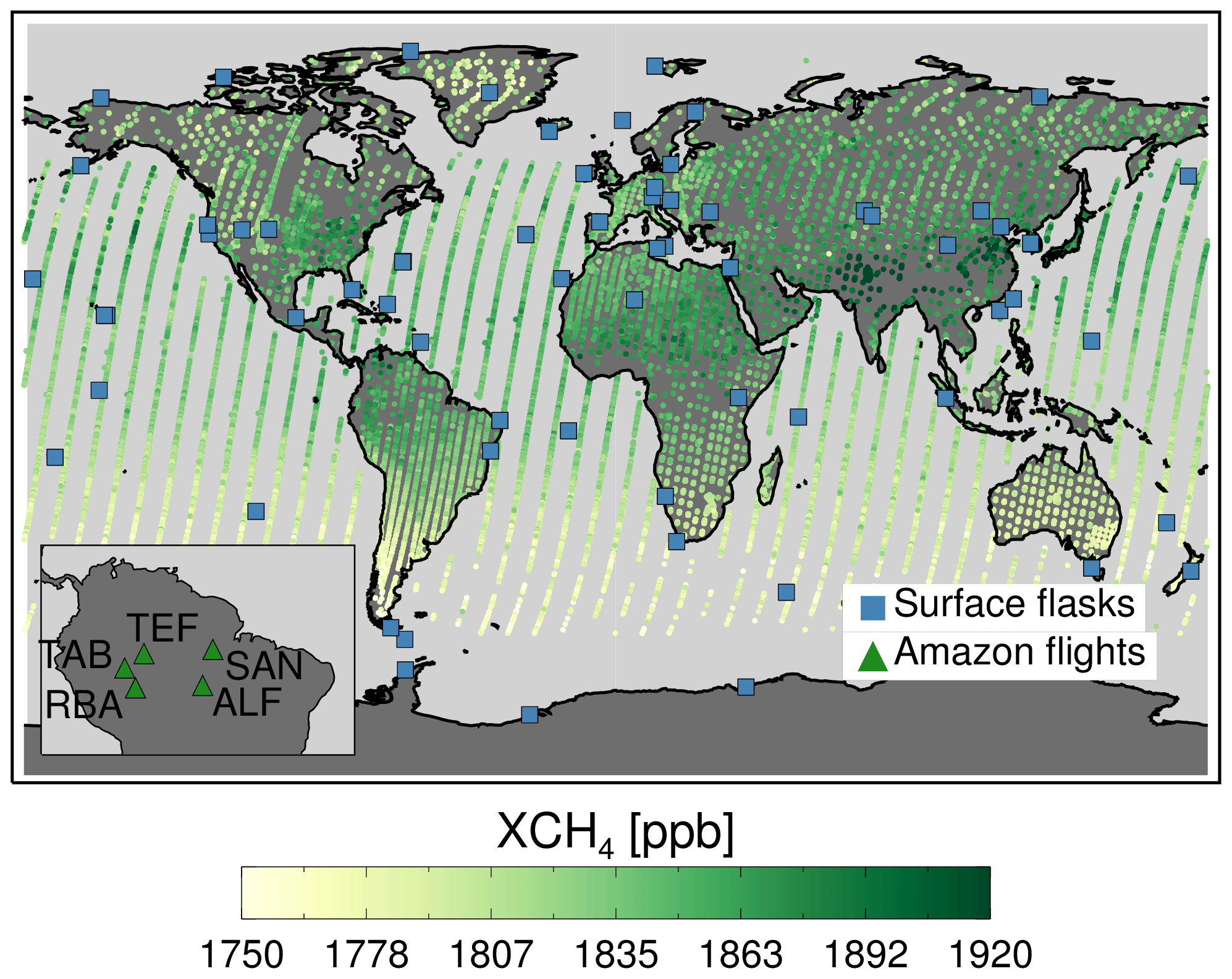
Figure 1Locations of NOAA surface sites from which flask-based measurements of CH4 are assimilated (blue squares), along with locations and values of GOSAT XCH4 retrievals for August 2017 (circles). Inset shows locations of flight-based observations of CH4 within the Amazon basin (green triangles).
2.1.1 Surface flask observations
We assimilate global long-term surface data of CH4 provided by the National Oceanic and Atmospheric Administration's Global Monitoring Laboratory (NOAA GML, Table A1 in the Appendix). We use data from 56 background monitoring sites, the locations of which are shown in Fig. 1. Whole air samples in flasks are collected weekly to biweekly (every 2 weeks) at each site, and CH4 is measured using gas chromatography with a flame ionisation detection method (Dlugokencky et al., 2018). Data from these sites are assimilated in order to constrain the background variations in CH4 mole fractions at the Earth's surface. The observations made at these locations have high accuracy but are generally located in regions that are not near significant sources of CH4. There is a relative lack of regular observation in tropical regions, where CH4 emissions are significant and uncertain. These observations can therefore provide accurate values for background CH4 mixing ratios but are not usually able to provide accurate regional CH4 distributions in those areas that require the most constraint.
2.1.2 GOSAT observations
We also assimilate column-averaged dry-air mole fractions of CH4 (XCH4) from the University of Leicester Proxy retrieval scheme v7.2 for GOSAT (Parker et al., 2011, 2020a). This dataset has been used in the past in forward modelling studies to assess wetland CH4 emissions using the TOMCAT model (Parker et al., 2018, 2020b). The GOSAT Proxy scheme uses the ratio of the retrieved XCO2 and XCH4, together with model-based estimates of XCO2, in order to reduce the effects of atmospheric scattering and improve coverage of XCH4 retrievals. This is particularly true in tropical land regions where the prevalence of cloudy pixels often restricts the successful direct retrieval of XCH4. GOSAT XCH4 retrievals have been used previously in a number of forward and inverse modelling studies (Fraser et al., 2013; McNorton et al., 2016; Feng et al., 2017; Miller et al., 2019). The observations are regularly validated against independent data, including CH4 observations made as part of the Total Carbon Column Observing Network (TCCON, Wunch et al., 2011), although none of the measurement sites included as part of this network are located within the Amazon region. Webb et al. (2016) compared GOSAT XCH4 to vertical profiles of flask-based measurements of CH4 taken at a number of sites within the Amazon basin (described here in Sect. 2.1.3) and found that biases between the satellite retrievals and the flask observations were not significantly different from zero.
Before assimilation, GOSAT-retrieved and a priori XCH4 were averaged onto the model grid. Both sun-glint observations over the oceans and nadir observations over land were included in the inversion. All XCH4 values measured by the satellite during one model time step in the same grid cell were averaged using a weighted mean according to their uncertainties. The largest number of observations combined into a single value was 32, and the mean number was 4.7 over land and 6.0 over oceans. Within the Amazon basin, the mean number of observations combined was 3.8. Figure 1 shows an example monthly distribution of observations used in the inversion. For accurate comparison between the retrieved XCH4 and those simulated by the model, GOSAT averaging kernels falling in the same model grid cell and time step were averaged, similarly to the XCH4, and applied to the model vertical profile. Using a single model profile in each grid cell and model time step allows the use of averaging kernels that have been averaged in this way without introducing a bias, due to the distributive property of matrix multiplication. Retrievals where the model and satellite surface pressure differed by more than 50 hPa were rejected.
Due to a range of potential error sources in both the atmospheric transport model and the GOSAT retrievals, there is a persistent bias between them, which varies with latitude. We quantified this bias by comparing the results of a previous inversion, in which only the surface flask observations had been assimilated for the full 2009–2018 period, to the GOSAT XCH4. We applied the averaging kernels to the three-dimensional (3-D) CH4 output from the flask data inversion and calculated the model–observation zonal mean bias B(φ), in parts per billion (ppb), as a function of latitude (φ), over this period:
where φ is equal to the latitude of the observation in degrees north (see Fig. A1). Positive values of B(φ) indicate positive observation bias relative to the model. Including a function that is constant along the longitudinal and temporal axes means that all information content from the satellite data along these axes is preserved, but this method reduces conflict between assimilation of the satellite and flask observations. Similar methods have been used before, for example in Bergamaschi et al. (2009). Across the tropics (30∘ S–30∘ N), the derived bias varies between 2.8 and 8.8 ppb. Further south, the bias reaches values up to 13.4 ppb. In our analysis we add the estimated bias value to the simulated XCH4 values in the inversion after the averaging kernels are applied.
2.1.3 Amazonian aircraft profiles
We used independent in situ observations of CH4 mole fraction made within the basin to validate our inversion results. Since 2010, aircraft-borne flask air observations of a number of species, including CH4, CO2 and carbon monoxide (CO), have been made at five locations within the Amazon basin (shown in Fig. 1, inset) by researchers at the Instituto de Pesquisas Energéticas e Nucleares (IPEN) in Sao Paulo, Brazil, until 2014 and at the National Institute for Space Research (INPE) São José dos Campos, Brazil (2015–present). The sites are located at Santarém (SAN, 2.9∘ S, 55.0∘ W), Tabatinga (TAB, 6.0∘ S, 69.7∘ W), Alta Floresta (ALF, 8.9∘ S, 56.7∘ W), Rio Branco (RBA, 9.3∘ S, 67.9∘ W) and Tefé (TEF, 3.6∘ S, 66.5∘ W). Measurements were only ever made concurrently at four locations, as the measurements at Tefé were started in 2013, to replace those made at Tabatinga up to 2012. We therefore combine observations made at these locations and refer to them as TAB/TEF throughout this paper. Both sites are located in the north-west of the Amazon basin and sample similar incoming air masses. Flights are undertaken at approximately biweekly (every 2 weeks) intervals above each site up to an altitude of ∼ 4.4 km, and 0.7 L flasks were filled every 300–500 m to produce vertical profiles. All measurements were taken between 12:00 and 13:00 local time, when the boundary layer is fully developed. The flasks were analysed for CH4 mole fractions at the high-precision gas analytics laboratory at IPEN and INPE, following the NOAA GML approach, including rigorous calibration to the World Meteorological Organization (WMO) CH4 mole fraction scale. The measurement locations were chosen in order to sample the dominant tropospheric airstream across the basin. These observations were not assimilated in the inversion. For more information about these measurements, see Gatti et al. (2014) and Basso et al. (2016).
2.2 Model set-up
2.2.1 Inverse model set-up
The TOMCAT model is a global 3-D Eulerian offline chemical transport model (CTM) (Chipperfield, 2006; Monks et al., 2017). It has been used in a number of previous studies of atmospheric composition and transport (e.g. Wilson et al., 2016; McNorton et al., 2016; Parker et al., 2018). We use the INVICAT inversion framework (Wilson et al., 2014), which is based on the TOMCAT model and its adjoint. INVICAT uses a variational scheme based on 4D-Var methods used in Numerical Weather Prediction (NWP) and has been used in the past to constrain emissions of species including CO2, ethane (C2H6) and nitrous oxide (N2O) (Gloor et al., 2018; Monks et al., 2018; Thompson et al., 2019; Tian et al., 2020). The inverse method employed by INVICAT is described in depth in these previous references. In brief, the method aims to minimise, in a least-squares sense, the value of a cost function. The cost function is an error-weighted sum of the model–observation mismatch, plus error-weighted departures from the a priori flux estimate.
The inversion input is in the form of an a priori mean flux value for each grid cell along with an error covariance matrix for these values, and the output is an a posteriori mean grid cell flux value and error covariance matrix. Mean a priori and a posteriori atmospheric mole fractions of CH4 are also produced. For brevity, throughout the remainder of this text, we will refer to the mean a priori and a posteriori fluxes as “prior fluxes” and “posterior fluxes”, respectively. Similarly, the mean a priori and a posteriori mole fractions will be referred to as prior and posterior mole fractions.
The forward and adjoint model simulations were carried out at 5.6∘ × 5.6∘ horizontal resolution, with 60 vertical levels up to 0.1 hPa. The model time step was 30 min. The meteorology was taken from the European Centre for Medium-Range Weather Forecasts (ECMWF) ERA-Interim reanalyses (ERA-I, Dee et al., 2011). The inversions were carried out for each year separately and each completed 40 minimisation iterations. For each year's inversion, 40 iterations were enough for the cost function and its gradient norm to be judged to have converged (less than 1 % variation through 5 consecutive iterations). The inversion for each year was actually run for 14 months up to the end of February for the following year, with the final 2 months being discarded from the results. This was in order to better constrain fluxes during the final months of each year. Each inversion therefore overlapped with the following one for 2 months but was initialised using 3-D fields provided from the correct date in the previous year, so that total CH4 burden was conserved across years.
For the assimilated surface observations, the model output was linearly interpolated to the correct longitude, latitude and altitude at the nearest model time step. For the averaged GOSAT observations, the model mole fractions were interpolated to the correct longitude and latitude at the nearest time step, before the GOSAT averaging kernels were applied to the model output to give an XCH4 value comparable with GOSAT. GOSAT observations are given an uncorrelated uncertainty equal to 2.5 times the supplied retrieval error, which ranged from 3.5 to 25.8 ppb, in order to account for representation error and observation correlations removed by the averaging of the retrievals, as in Chevallier (2007). This inflation value was based on the mean number of observations combined in each grid cell. In short sensitivity tests, the magnitude of posterior emissions was not sensitive to this inflation factor once it was larger than 2, although the posterior error estimate was affected. This choice gave a mean GOSAT XCH4 uncertainty value of 24.4 ppb. NOAA observations are given uncorrelated errors of 3 ppb plus representation error. For these observations, representation error was estimated as the mean difference across the eight grid cells surrounding the cell containing the observation location.
Prior emissions are given grid cell uncertainties of 250 % of the prior flux value but also included spatial and temporal correlations. Although inversions such as this do not directly allow for sectorial analysis of emissions, we use the off-diagonal values of the prior covariance matrix to provide some information of this nature. Similar to Meirink et al. (2008), we split our prior and posterior solutions into the anthropogenic fossil fuel emissions assumed to be strongly correlated in time (FF), as well as emissions with strong seasonal cycles from natural, agricultural and biomass burning sources (NAT + AGR + BB) by imposing prior temporal correlations on the FF contributions. FF emissions in each grid cell in each month were correlated with emissions from the same grid cell in other months with an exponential correlation function with a timescale of 9.5 months (equivalent to a consecutive-month correlation of 0.9). Both NAT + AGR + BB and FF sectors had spatial correlations imposed between grid cells, based on Gaussian covariance functions with correlation length scales of 500 km. This gives global uncertainty of approximately 70 Tg yr−1. The sectors which make up the NAT + AGR + BB and FF emissions are explained in Sect. 2.2.2.
We produced estimates for each year's posterior emission covariance error matrix using cost function gradient values from the limited-memory Broyden–Fletcher–Goldfarb–Shanno algorithm (L-BFGS) that we employ to minimise the cost function (Nocedal, 1980), based on the method suggested by Bousserez et al. (2015). This iterative method estimates the inverse of the Hessian (the second derivative) of the cost function and does not include the off-diagonal elements of the posterior covariance matrix, so the posterior errors described in this paper are likely to be lower limits (Bousserez et al., 2015).
2.2.2 Prior emissions and chemical sinks of CH4
Prior emissions were taken from a range of widely available bottom-up models and inventories. Anthropogenic emissions were originally taken from the EDGAR v4.2 FT 2010 inventory (Olivier et al., 2012) and scaled as in McNorton et al. (2018) to apply an increasing global linear trend for the period after 2012. Biomass burning emissions were taken from GFEDv4.2 (van der Werf et al., 2017). The JULES model (Clark et al., 2011) was used to provide wetland fluxes, in a configuration described in McNorton et al. (2016), using four separate carbon pools to drive methanogenesis. Rice emissions were taken from Yan et al. (2009) and are scaled by a factor of 0.75 as in Patra et al. (2011). Remaining small natural sources (termites, geological and oceanic emissions) were included as in Wilson et al. (2016). Sectoral emission maps are shown in Fig. A2, whilst prior totals for each source type within South American regions are shown in Table 1. The prior global flux of CH4 to the atmosphere rises from 549.5 Tg yr−1 in 2009 to 564.0 Tg yr−1 in 2017. The surface soil sink due to methanotrophs was from the Soil Methanotrophy Model (MeMo, Murguia-Flores et al., 2018), repeating the 2009 flux every year, with a value of 33.9 Tg yr−1. Landfill and fossil fuel emissions had temporal correlations imposed in the prior uncertainty matrix and made up the FF category, whilst the remaining emissions (NAT + AGR + BB) had no prior temporal correlations imposed. Atmospheric OH fields, based on those provided within the TransCom CH4 study (Patra et al., 2011), were taken from Spivakovsky et al. (2000) and scaled downwards by 8 % in accordance with Huijnen et al. (2010). The OH fields used here have previously been shown to capture observed atmospheric lifetimes for CH4 and methyl chloroform (CH3CCl3) in TOMCAT to within the observed uncertainty, although simulations of sulfur hexafluoride (SF6) and other species show that the interhemispheric gradient in TOMCAT is slightly large compared to observations but within the bounds of other transport models (Patra et al., 2011; Wilson et al., 2014). The OH fields vary from month to month but do not vary between years. Montzka et al. (2011), Naus et al. (2020) and Patra et al. (2021) suggested that variability in annual OH mole fractions is small, but other recent research has suggested the possibility of a declining trend in OH since 2004 (Rigby et al., 2017; Turner et al., 2017), although this trend had a high level of uncertainty. Other studies have found that the El Niño–Southern Oscillation (ENSO) has had a significant impact on OH variability in the troposphere in recent decades (e.g. Rowlinson et al., 2019; Anderson et al., 2020; Zhao et al., 2020), and potentially an increasing trend in tropospheric OH during 1980–2010 (Zhao et al., 2020). A trend in OH, or any year-to-year variability, was not included in our analysis, which will inform our conclusions, but for now we do not have enough evidence to include any potential variations. Stratospheric loss fields due to reactions with atomic chlorine (Cl) and excited oxygen atoms (O(1D)) varied on a monthly and annual basis and were taken from a previous full chemistry simulation from TOMCAT (Monks et al., 2017). The total simulated atmospheric CH4 sink due to reaction with the OH radical in 2009 was 494.5 Tg, whilst the annual stratospheric CH4 sink due to O(1D) and Cl was 19.5 Tg. CH4 loss in the troposphere through reaction with Cl was not included in these simulations.
2.2.3 Bottom-up model
We also use a simple bottom-up (B-U) model to estimate wetland CH4 emissions from meteorological and ecological input data, so that we can investigate the causes of variations in CH4 emissions derived in the inversion. The B-U model, which is based on observed or modelled estimates of wetland fraction, heterotrophic respiration of carbon and surface temperature, is described fully in Appendix B. The model uses measurements of gravity anomalies made on the twin Gravity Recovery and Climate Experiment (GRACE) satellite mission as a proxy for variations in wetland fraction. The equation that our B-U model is based on is commonly used in other studies that estimate wetland fluxes of CH4 (e.g. Clark et al., 2011; Melton et al., 2013; Bloom et al., 2017), but our application of the driving climate variables is fairly simple relative to these previous works. This method is sufficient for this work as the purpose of the B-U model is to investigate the possibility of reproducing the inversion results, and if they can be reproduced, to learn how and why the CH4 wetland emissions change according to the input variables. If the inversion results are not reproduced using the B-U wetland model, it could indicate that other sectors played a role in any observed variation.
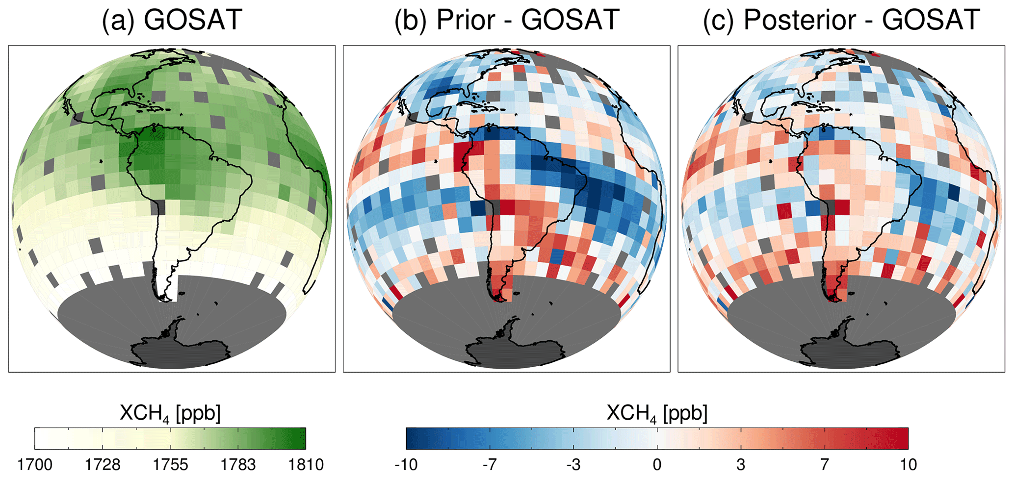
Figure 2(a) Mean GOSAT XCH4 over South America and surrounding area for 2009–2018. Observations have been averaged onto the TOMCAT model grid as described in the text. Also shown is the mean difference between the model and satellite XCH4 using (b) the prior emissions and (c) the posterior emissions for the same period.
3.1 Average distribution of emissions
Average GOSAT XCH4 values over South America since 2009 show that XCH4 column mole fractions were largest over the west of the continent, particularly in the north-west (Fig. 2). Using the prior flux distribution in TOMCAT leads the model to underestimate XCH4 in the north-east and far north of the continent and in the outflow into the Atlantic Ocean. Simulated XCH4 is overestimated to the south and west of the continent. After assimilation, the largest model biases are removed, although there is a small positive bias in the interior of the continent, usually smaller than 5 ppb. The posterior (prior) mean model–satellite mismatch, weighted by the observation uncertainty, is 0.2 (−24.1) ppb globally, −5.4 (−40.0) ppb within South America and −4.1 (−66.5) ppb within the Amazon basin. The posterior residuals show no significant trend or seasonality within South America or within the basin (Fig. A3).

Figure 3Prior, posterior and (prior–posterior) mean gridded total South American CH4 emissions (mg m−2 d−1) for the period 2009–2018 (a–c), and similar but for fossil fuel sources (d–f) and natural/agricultural/biomass burning sources (g–i) only.
Figure 3 shows the 2009–2018 mean prior and posterior emission distributions of CH4 emissions in South America. We display the mean over this entire period in order to show the consistent, long-term emission distribution. Whilst posterior uncertainty in particular grid cells can still be fairly large (Fig. A4), regional changes are much less uncertain. Posterior South American emissions are significantly redistributed compared to the prior distribution due to changes in the NAT + AGR + BB emission sectors. Whilst the prior emissions are fairly homogeneous across much of the Brazilian Amazon, the posterior emissions are largest to the north-east of the continent and are reduced in the south and the north-west. Emission rates in the far north of the continent, potentially related to seasonal flooding in the basin of the Orinoco river in Venezuela, are also high in the posterior results.
The most significant feature of the posterior distribution is a region of high emission rates near the coastal basins around the mouth of the Amazon River itself (Fig. 3). There are large emissions from the region around the north-eastern states of Para, Maranhão and Tocantins. These areas contain the basins of many of the larger Amazon tributaries and a high density of wetland sources such as marshes, swamps and mangroves, according to the Sustainable Wetlands Adaptation and Mitigation Program (SWAMP) data from the Center for International Forestry Research (CIFOR) (Gumbricht et al., 2017). The prior flux distribution also highlights agricultural sources near this region in the EDGAR inventory (Fig. A2).
However, in our posterior results, the western Amazon and the Pantanal region in the south of Brazil do not display high emissions. Although the coarse resolution of the model grid boxes masks the signal from the relatively small Pantanal region in the prior emissions to some extent, it is still surprising that the posterior emissions have small methane fluxes from the southern regions of Brazil. As shown in Fig. 2, the model generally overestimates the XCH4 in southern Brazil compared to GOSAT when using the prior emissions, so it is not surprising that emissions from that region were reduced in the inversion. The low emissions from a region where we expect significant methane release might mean that the model transport errors affect comparisons in this region, that the model–satellite bias included in the inversion (Eq. 1) is inaccurate or that the GOSAT sampling does not cover this region well (note the relatively small error reduction in this region, Fig. A4). The low emissions in the western Amazon are also a consistent feature of our results. The FF emissions do not change significantly in the inversion, although they are slightly decreased towards the south-east of Brazil, close to the large cities of São Paulo and Rio de Janeiro. The overall pattern of the posterior emissions displayed in Fig. 3 is robust on a year-to-year basis, with the change relative to the prior in each individual year displaying very similar patterns to the multi-year mean (Fig. A5).
Table 1Prior and posterior emissions of CH4 for Brazil and other subregions of South America (2010–2017). Units are Tg yr−1.
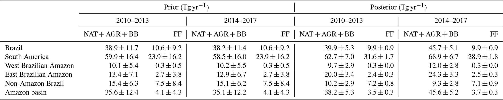
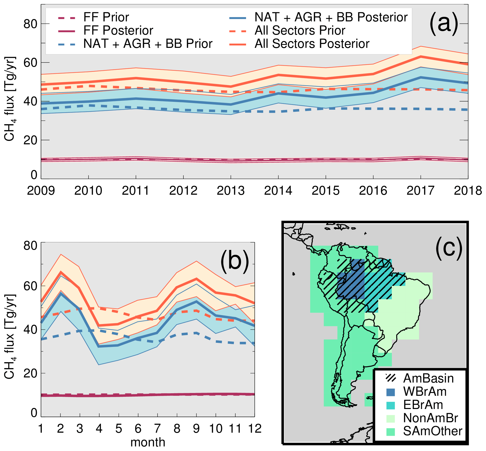
Figure 4(a) Total annual Brazilian prior and posterior emissions (Tg(CH4)/yr). Shaded areas show posterior uncertainties as derived in the inversion. (b) Monthly mean prior and posterior Brazilian CH4 emissions (Tg(CH4)/yr, 2009–2018). Shaded areas show the standard deviation for each month. (c) Regions of South America discussed in the text. The hatched area (AmBasin) represents the Amazon basin across all countries, whilst the shaded areas show Brazilian and non-Brazilian regions.
3.2 Temporal variations of CH4 emissions
The annual total prior emissions in Brazil are nearly constant over time (Fig. 4), with a mean value of 48.6 ± 14.9 Tg yr−1 (uncertainty here from prior error covariance matrix). However, the posterior emissions show a positive trend, particularly from 2013 onwards. Globally, the posterior flux rises from 566.2 Tg yr−1 in 2009–2013 to 594.0 Tg yr−1 in 2014–2018 (Table 1), consistent with other studies (e.g. Saunois et al., 2020). In Brazil, the mean posterior annual emissions are 49.8 ± 5.4 Tg yr−1 in the period 2009–2013 but rise to 55.6 ± 5.2 Tg yr−1 in 2014–2018, with a mean value over the whole period of 52.7 ± 5.3 Tg yr−1. The uncertainty stated for these figures represents the overall mean annual posterior uncertainty for Brazil derived in the inversion for each 4-year period. We report the mean annual uncertainty as we assume that posterior uncertainty for each year is strongly correlated with that in other years. Reporting the mean value implicitly assumes a correlation of 1 between the years' uncertainties; in reality the correlation is likely smaller than 1. Our total Brazilian mean flux is within the range found by Saunois et al. (2020) and agrees well with the findings of Janardanan et al. (2020). There is a significant positive trend over the whole time period (2010–2018) of 1.37 ± 0.69 Tg yr−2 (p<0.05), driven by the NAT + AGR + BB emissions category, although the distribution actually resembles a step change in 2014.
Posterior emissions in Brazil peak in February and September (Fig. 4b), representing the wet season and dry season, most likely due to contributions from the local seasonal cycles of wetland emissions and biomass burning emissions, depending on the location. The peak monthly emission rate of 66.2 ± 8.2 Tg yr−1 is in February, before lower rates of emission during April to July. This February peak corresponds to a peak in precipitation across the basin (from the Global Precipitation Climatology Project (GPCP) v2.3 combined precipitation dataset, Adler et al., 2018) but precedes the peak in gravity anomaly – representative of soil water depth – captured by the GRACE satellite (Fig. A6). Emissions in August and September are almost as large as those during the peak of the wet season. Again, almost all of this seasonal variation comes from the NAT + AGR + BB emission category.

Figure 5(a–c) Total annual (red lines) prior and posterior emissions of CH4 (Tg yr−1) in three Brazilian subregions: the western Brazilian Amazon (WBrAm), the eastern Brazilian Amazon (EBrAm) and non-Amazon Brazil (NonAmBr). Prior and posterior emissions during the wet season (December–March, grey lines) and the dry season (August–October, maroon lines) are also shown. Shading represents the posterior uncertainties for each region derived in the inversion. (d–f) Monthly mean prior and posterior emissions for the period 2009–2018 (Tg yr−1) for the three subregions. Shading shows the standard deviation of the monthly means.
Within the entire Amazon region, emissions grew from 41.7 ± 5.3 Tg yr−1 in 2010–2013 to 49.3 ± 5.1 Tg yr−1 in 2014–2017. Emissions are largest in the eastern Brazilian Amazon (EBrAm, Fig. 5) and are significantly larger than suggested by the prior emissions, particularly in the most recent years. The increase in emissions over the period is also largest there, rising from 22.4 ± 3.4 Tg yr−1 in 2010–2013 to 26.8 ± 3.3 Tg yr−1 in 2014–2017 (trend: 1.06 Tg yr−2, p<0.01). Emissions also increase from 10.0 ± 2.9 Tg yr−1 to 12.3 ± 2.8 Tg yr−1 between these two periods in the western Brazilian Amazon (WBrAm). However, in the non-Amazon region of Brazil (NonAmBr), emissions decrease slightly over these years (from 17.5 ± 3.0 to 16.4 ± 2.9 Tg yr−1). Trends in WBrAm and NonAmBr are not significant for p<0.01. The Amazon regions of Brazil display the two-peak seasonal cycle of CH4 emissions, although this is much more pronounced in the east. This is at least partly due to the significant effect of biomass burning within the arc of deforestation in the south-east of the basin that usually occurs during these months. Emissions are largest in NonAmBr during the dry season, possibly due to fires or agricultural activity.
We also show total emissions for each subregion during the wet season (December–March) and the dry season (August–October). These periods were defined using the GPCP precipitation data, as periods when the average monthly precipitation during 2009–2018 within the basin was more than 7 mm d−1 and less than 3 mm d−1, respectively. In both WBrAm and EBrAm, the trends for the 2009–2018 period are largest in the wet season. This suggests that trends in wetland and floodplain emissions could be responsible for the rising CH4 emissions, in line with reports of intensifying flood extremes in the area in recent decades (Barichivich et al., 2018). However, there are other potential explanations. These include escalating biomass burning emissions during the wet season (Silva Junior et al., 2019) and an intensification of agricultural emissions in these regions, as seen in version 5.0 of the EDGAR anthropogenic flux inventory in Brazil (Crippa et al., 2020), or some combination of factors. Unfortunately, our results cannot be used to say more about which sectors are responsible for the increasing flux.
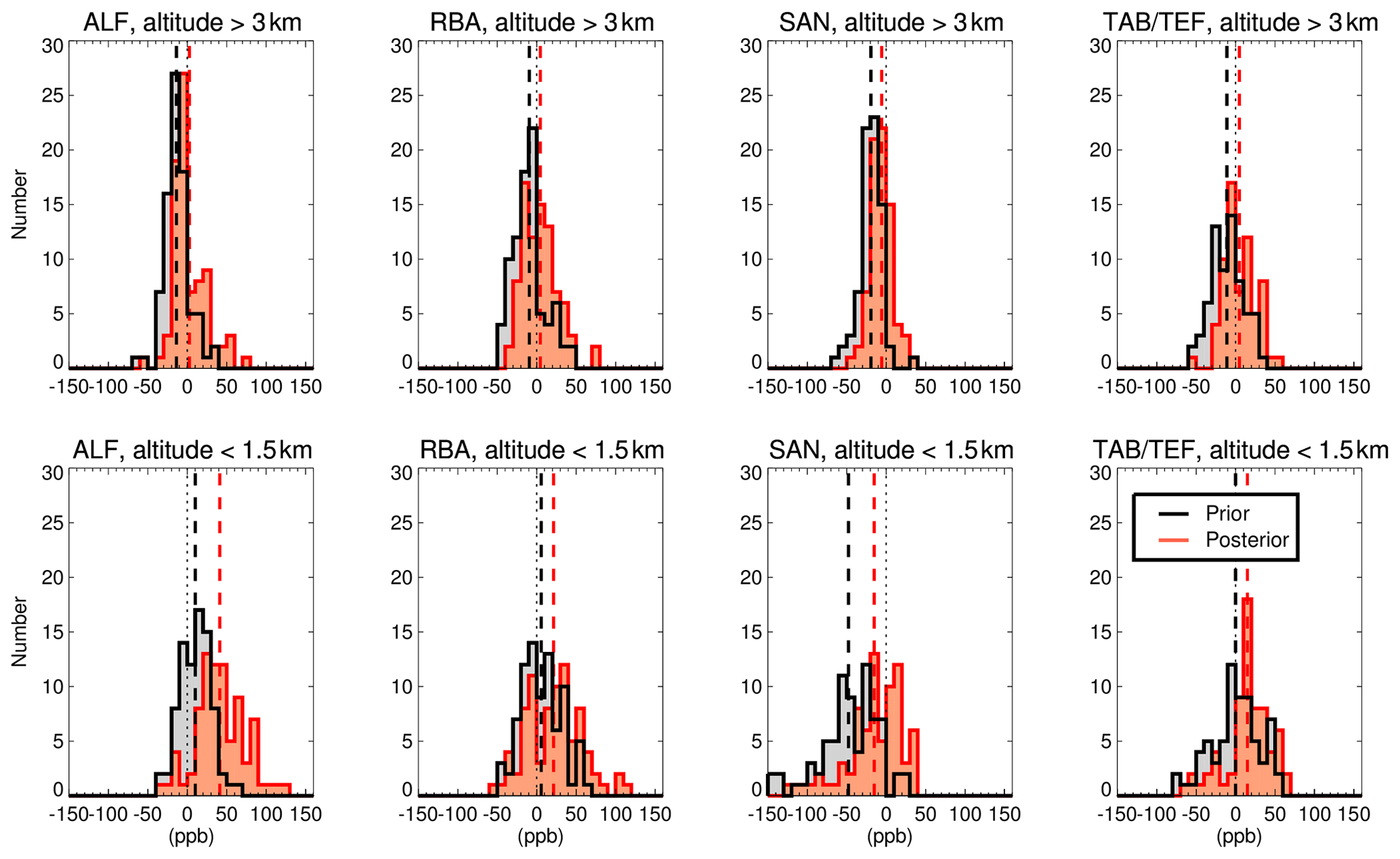
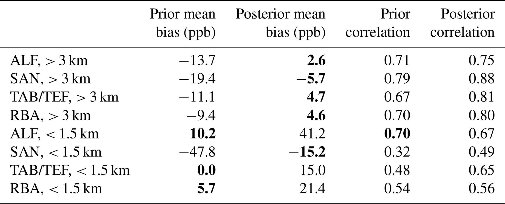
Figure 6Histogram plots showing prior (black) and posterior (red) (model–observation) differences at the four Amazon flight locations, 2010–2018. Measurements were taken at Alta Floresta (ALF), Rio Branco (RBA), Santarém (SAN), and Tabatinga and Tefé (TAB/TEF). Model output has been interpolated to observation locations and altitudes, before both were averaged into monthly means and into altitude bins of 3 km and above (a–d) and 1.5 km and below (e–h). Dotted vertical lines show the zero line, whilst dashed vertical lines show prior and posterior mean model–observation bias.
3.3 Comparison to independent observations
Observations of CH4 made during flights within the basin between 2010 and 2018 were used to independently check the performance of the prior and posterior emission distributions in the model (Fig. 6, Table 2). For the observations made at altitudes higher than 3 km, which represents the free troposphere above the Amazon, the mean bias (MB) between model using the posterior emissions and the observations is significantly reduced at all locations, compared to that produced when using the prior flux in the model. The correlation between the model and the observations also increases at all locations when using the posterior flux rather than the prior. The absolute value of the model–observation bias is reduced to below 6 ppb at all sites. However, the posterior model MB against observations made in the boundary layer, at altitudes below 1.5 km, is higher than the prior model MB at three sites. At the western sites, RBA and TAB/TEF, the MB in the model increases by approximately 15 ppb, although the correlation improves, particularly at TAB/TEF. At ALF, the correlation decreases slightly, and the MB increases by a large amount (31 ppb). Finally, at SAN, the performance improves significantly by both measures, with the MB being reduced from −47.8 to −15.2 ppb. There are no significant trends (at 95 % level) in the model–aircraft residual biases in 2010–2017, except at TAB/TEF below 1.5 km. This site has a posterior residual bias trend of +2.1 ppb/yr, but this may have been caused by the change in the flight location halfway through the study period.
The improved performance at SAN is significant, as the high mole fractions of CH4 sampled at this location relative to expectations given its location situated close to the eastern coast have been previously noted (Miller et al., 2007; Basso et al., 2016; Wilson et al., 2016). The prior model therefore has a large negative bias at SAN, particularly near the surface. The posterior distribution of emissions, with a region of high emission rates to the south and east of the basin, substantially reduces the model–observation difference at SAN. The model still underestimates methane mole fractions at this site even after the improvement, however, which might be due to bias which remains in the posterior flux estimate, possibly due to the allocated prior uncertainty in this region being too small, or model representation uncertainty. The fact that ALF is also located near these significant emissions leads to degradation in the model performance within the boundary layer, which was previously better at ALF than at SAN. The capability of assimilation of GOSAT XCH4 to improve performance at both of these locations might have been reduced due to the relatively coarse model grid. Webb et al. (2016) found that comparisons between the flight-based observations and a previous version of the GOSAT XCH4 used in this study showed that the GOSAT values were larger than equivalents estimated using the flight data at ALF but that the discrepancy was much smaller at SAN. This being the case, it is not surprising that the model in which the GOSAT data have been assimilated has difficulties in matching the flight observations at both locations at once. Since we assimilated XCH4 from GOSAT, which is mostly representative of the troposphere, it is expected that the model performance is improved at all locations when compared to observations made at the higher altitudes. This also indicates good model representation of inflow of CH4 to the basin from elsewhere. However, the fact that the posterior comparisons are generally degraded close to the surface, apart from at SAN, means that the local sources close to these sites might be overestimated at this model resolution, that there are errors in the model's representation of vertical mixing or that there remains a positive bias in the assimilated retrievals from GOSAT in this region. Generally, however, the temporal variation and MB in the model is much improved after the assimilation of GOSAT XCH4.
Table 2Prior and posterior bias (ppb) and correlation between TOMCAT and Amazon flight observations (2010–2018). The better value for bias and correlation for each site and altitude is highlighted in bold.
3.4 Bottom-up model results
The inversion suggests that CH4 emissions have been significantly increasing from eastern Amazon regions throughout the 2010s, but it is not able to determine the source sectors responsible for this rise. The largest increases over time occur during the wet season (Fig. 5), when wetland emissions dominate the atmospheric signal, so it is possible that changes to these emissions led to the increase. Emissions from seasonal floodplains and wetlands are sensitive to temperature, precipitation (which affects wetland area) and carbon availability in the soil (Bloom et al., 2017), so we examined these factors to see how they varied during the previous decade and whether wetlands could have been responsible for increasing wet season CH4 emission in the basin.
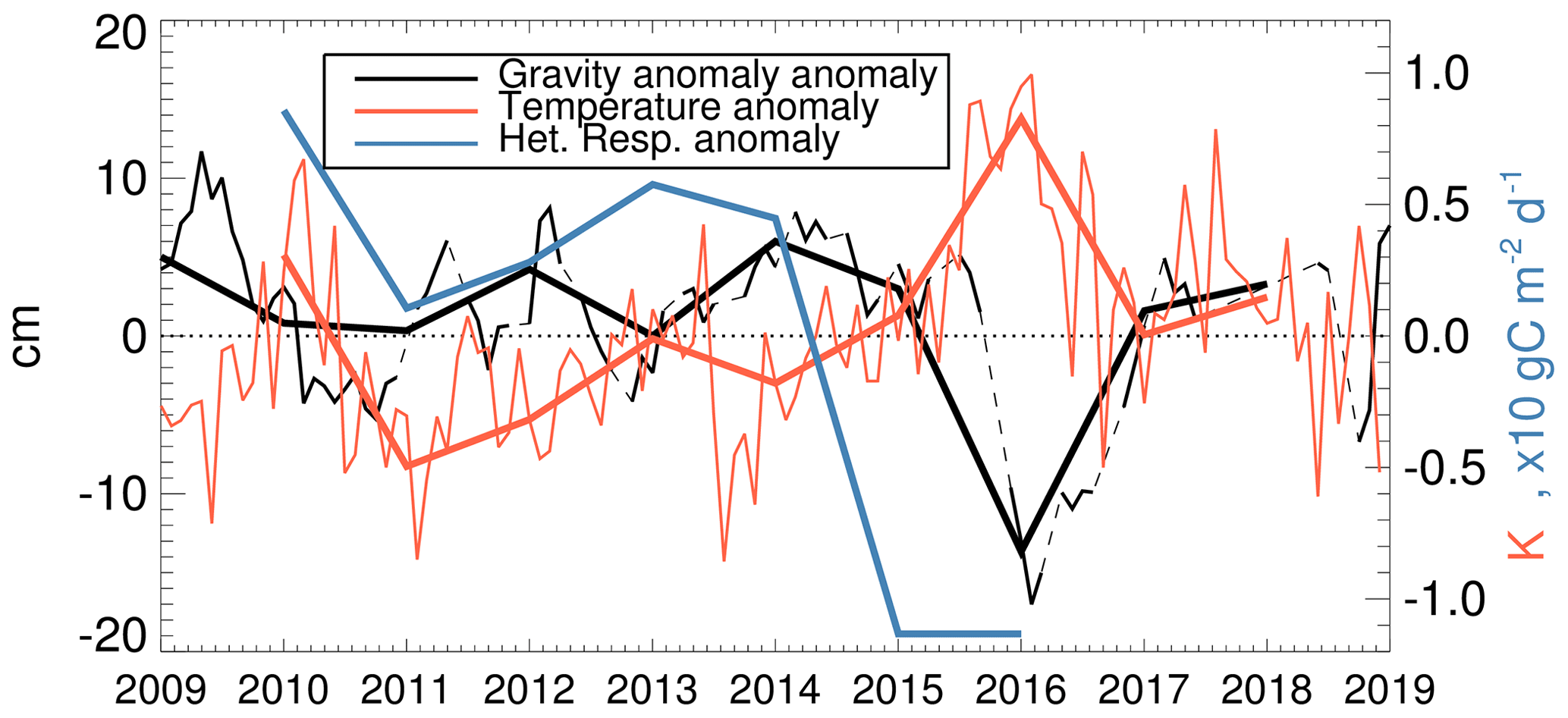
Figure 7Anomalies of gravity anomaly (cm, black, left axis), surface temperature (K, red, right axis) and heterotrophic respiration (×10 gC m−2 d−1, blue, right axis) for the period 2009–2018 within the Amazon basin. Monthly mean anomalies are shown as thin lines, whilst wet season (December–March) averages are shown as thick lines. Interpolated values for gravity anomalies are shown as dashed lines.
The mean surface temperature within the Amazon basin increased throughout the period 2009–2018 (Fig. 7), while there was no significant trend in precipitation (not shown) or gravity anomaly. Estimating the trends of these factors is significantly affected by one anomalously dry and hot period, running from late 2015 to mid-2016. These record-breaking conditions were caused by the 2015/16 El Niño and were largely confined to the east of the basin (Jiménez-Muñoz et al., 2016). A previous extreme event during this study period, in the dry season of 2010, displayed a similar geographical distribution but was easily surpassed by the scale of the 2016 drought (Lewis et al., 2011; Jiménez-Muñoz et al., 2016). One other event that stands out is the prolonged flooded period running through the wet season of 2013/14, during which rainfall in the south-west of the basin was up to twice as much as usual (Espinoza et al., 2014). This flooded period did not coincide with a significant ENSO period but was likely caused by warm conditions in the subtropical South Atlantic.
Figure 7 also shows the wet season mean anomalies for each year for the surface temperature, gravity anomaly and modelled heterotrophic respiration. Wet season temperatures were high in 2010 and in 2015, 2016 and 2018. The water table was at its highest in 2012, 2014 and 2015. Finally, heterotrophic respiration was strongest in 2010, 2013 and 2014 but very low in 2015 and 2016. There was no heterotrophic respiration model data available for 2017, so we used a climatology value for that year. We felt that this was justified since the temperature and water table depths also had only very small anomalies during that season. As might be expected, the temperature and gravity anomalies in the wet season were strongly negatively correlated (), due to coincidence of hot and dry conditions.
The temperature trend in the Amazon was positive throughout almost the entire basin (Fig. 8a), particularly in the far west and south-east. The trend in the wetland fraction (Fig. 8b) was more heterogeneous, with positive trends in the west contrasting with strong negative trends across the east of the basin. Both sets of trends are strongly impacted by the hot, dry conditions in 2015/16.
The geographical distribution of the NAT + AGR + BB wet season CH4 emission trend produced by the inversion (Fig. 8c) is positive across the north-west and south-east of the basin, with a similar distribution to the temperature trends. The positive emission trends in the north-west are collocated with an area of increasing wetland fraction. However, the regions to the east and south with strong positive emission trends are located where wetland fraction had been decreasing as temperatures increased. This suggests that, if wetlands were responsible for increased wet season flux, the methanogenesis must have been more sensitive to the increasing temperature than to the decrease in wetland fraction or in heterotrophic respiration (not shown).
We ran the B-U model multiple times, varying the temperature response and the GRACE anomaly scaling variables in order to produce a range of likely values for CH4 flux from the basin. We also optimised B-U model parameters, as described in Sect. 2.2.3, in order to best reproduce the INVICAT results using the B-U model (Fig. 8d and e). The B-U model combines the three driving variables, but the strong anti-correlation between the temperature and wetland fractions means that this model does not produce strong variations in emissions, since the two tend to cancel out. Using the optimised B-U model produces weak positive emission trends in the west of the basin and weak negative trends elsewhere, giving no significant trend overall (p=0.36). The optimised values are included in Appendix B. The standard deviation of the wet season emissions in the B-U model is 1.7 Tg yr−1, compared to 2.4 Tg yr−1 in the inversion results. The mean posterior error in the inversion results (2.9 Tg yr−1) is relatively large compared to the standard deviation, however, meaning that the B-U values almost always remain within the posterior inversion uncertainty. The exception to this is the wet season of 2014, when the inversion results produce larger emissions than in any other year (20.1 ± 2.7 Tg), and this feature is not reproduced by the B-U model. As discussed, the wet season of 2014 was subject to extreme precipitation and widespread flooding in the basin (Espinoza et al., 2014), and the GRACE gravity anomalies are large throughout this period (Fig. 7), whilst heterotrophic respiration was high and temperatures were relatively cool (although warmer than in 2011 and 2012). Despite these conditions which seem favourable to CH4 emission, the B-U model does not produce emissions significantly larger than any other year. The discrepancy between the inversion and B-U model results is discussed further in Sect. 4. Figure 8e also shows the wet season emissions within the basin from the full ensemble (FE) of the WetCHARTs emission dataset (Bloom et al., 2017), which use a similar method to estimate wetland emissions that used in our B-U model. These emissions also show a negative trend over the period 2010–2017 (−0.17 Tg yr−1), and the variation is again small (0.93 Tg yr−1 standard deviation). They display no significant change in emissions in the wet season of 2013/14. The implications of the discrepancy between the inversion and the B-U model are discussed in Sect. 4.
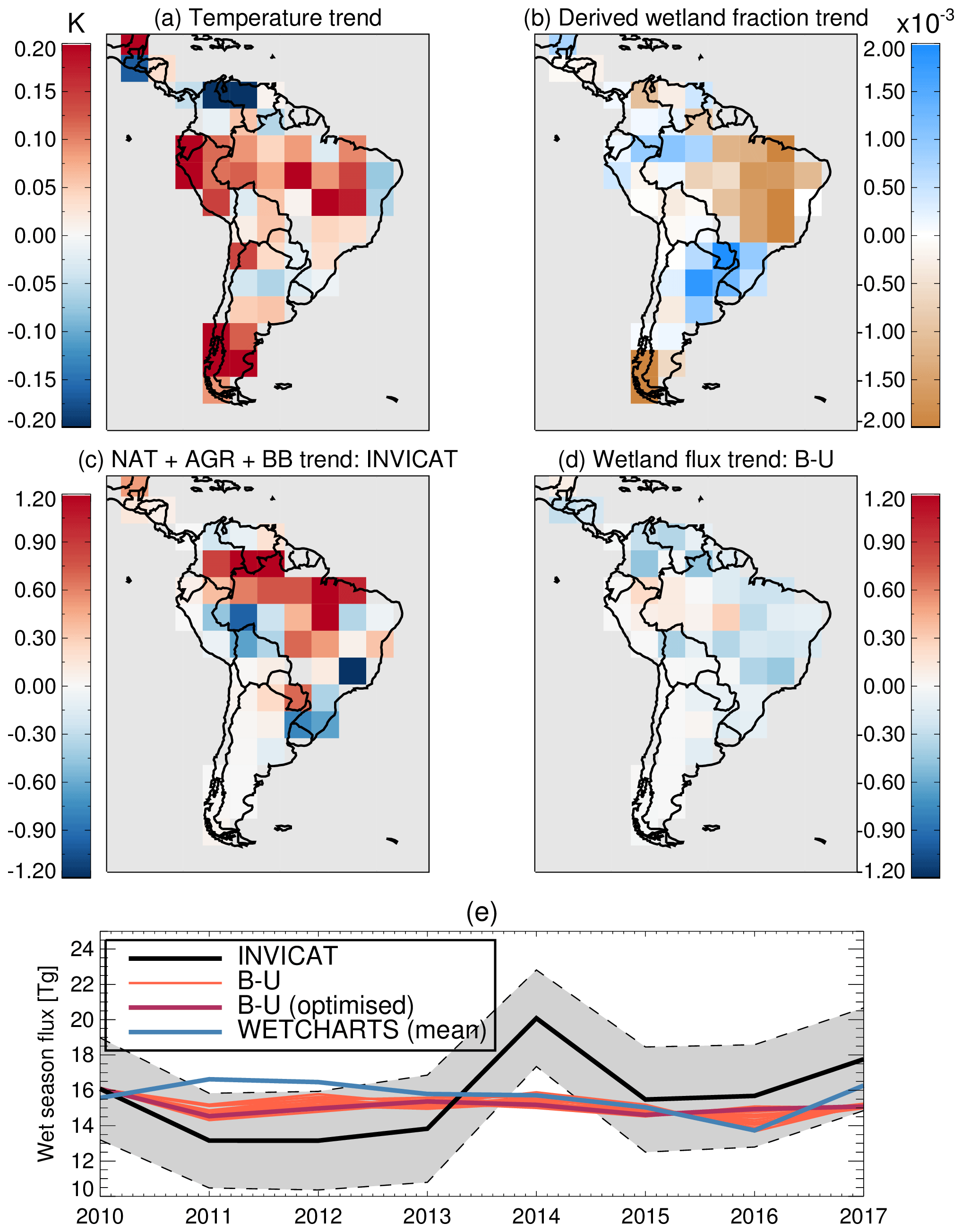
Figure 8Average wet season trends for the period 2010–2017 for the (a) temperature in K yr−1, (b) wetland fraction in 10−3 yr−1, (c) NAT + AGR + BB CH4 surface flux in mg m−2 d−1 yr−1 from GOSAT inversion and (d) optimised bottom-up (B-U) model surface flux of CH4 in mg m−2 d−1 yr−1. (e) Total Amazon basin wet season CH4 emissions in Tg (2010–2017) from GOSAT inversion (black line, with grey shading representing posterior uncertainty). Red lines show ensemble of B-U model simulations, and the maroon line is the optimised B-U model. The blue line shows the mean of the WetCHARTs full ensemble wet season flux.
We derive emissions of CH4 in Brazil for the period 2010–2018 of 52.7 ± 5.3 Tg yr−1, split into two periods during which mean Brazilian emissions were 49.8 ± 5.4 in 2010–2013 and 55.6 ± 5.2 in 2014–2017, an increase of 5.8 ± 5.2 Tg yr−1. This increase was found to be entirely due to the NAT + AGR + BB emissions within the Amazon region. In Amazonia, emissions grew from 41.7 ± 5.3 to 49.3 ± 5.1 Tg yr−1 over the same two periods.
This increase between the two periods is very similar to that found by Tunnicliffe et al. (2020), although the total emissions found in our study are larger than their finding of 33.3 ± 3.7 Tg yr−1. They removed a model–satellite bias of 22 ± 8 ppb from the GOSAT observations used in their study, which is much larger than our bias of 3–9 ppb removed from XCH4 over the Amazon. This treatment of bias, coupled with differences in model transport, could explain the different emissions derived. The positive biases in our posterior CH4 relative to aircraft observations within the boundary layer also suggest that our emissions could be overestimated. However, we note the absence of significant trends in our posterior model minus aircraft residuals between 2010–2017. Our posterior total emissions agree well with the findings of Janardanan et al., (2020), who derived Brazilian emissions of 56.2 ± 10 Tg yr−1 for the period 2011–2017, although temporal variation of this value was not discussed in that study. Yin et al. (2020) did not report total emissions but found a rise in Amazonian emissions of 4.2 ± 1.2 Tg yr−1 over 2010–2017, along with small increases in eastern Brazil. Our estimate of total flux from Amazonia agrees well with that of Pangala et al. (2017), who derived a total of 42.7 ± 5.6 Tg yr−1 for 2010–2013. A group of 22 inverse model experiments presented by Saunois et al. (2020) produced a range of 47.3–78.2 Tg yr−1 for Brazilian emissions between 2008 and 2017, although one of those results used the TOMCAT forward model to represent the atmospheric transport, so it is not fully independent from our results. Our findings here are within the range of these models, albeit towards the lower end. The majority of those top-down studies used either the same GOSAT and surface observation data used in our study or some variation of it. The fact that the derived emissions using similar observation data can vary so much highlights the inherent uncertainties still remaining in top-down studies of CH4 emissions, with differences in model transport, chemistry representation, inversion methodology, bias correction and error assumptions all contributing to differences in results.
The increase in emissions that we derive from 2014 onwards coincides with a faster rate of increase in the observed surface mole fraction of CH4 (Nisbet et al., 2019). Unfortunately, the extent that the increase in observed mole fractions in the atmosphere is driven by increasing Amazon emissions is difficult to constrain without more extensive knowledge of the atmospheric chemical loss of CH4. Our global inversion, using repeating OH values each year, indicates that the increase of 5.8 ± 5.2 Tg yr−1 from Amazon emissions is responsible for 24 ± 18 % of the global total increase in emissions between 2010–2013 and 2014–2017, which was 24.1 ± 15.0 Tg yr−1.
The Amazon emissions derived in this study for 2010 and 2011 (41.6 ± 5.3 Tg yr−1) are a little above the higher limit of those found in our previous study using the flight observations only (31.6–41.1 Tg yr−1, Wilson et al., 2016). This indicates that using the vertical profile data only to calculate basin-wide emission totals may lead to a small underestimation of the total compared to using satellite data. This discrepancy is supported by the positive bias seen in this study within the boundary layer at most of the sites when comparing the posterior model output to the in situ flight observations. However, the emission totals are fairly similar across the different methodologies, with the caveat that the same transport model was used for both findings.
The posterior fluxes lead to an improvement compared to the prior in the mean bias and correlation at all four independent sampling locations when only observations made above the boundary layer are considered. However, the posterior comparison to observations made close to the surface is inferior to the prior comparison at three of the locations. It seems that improving the performance compared to the GOSAT data throughout the troposphere is at the expense of diminishing performance at the surface. There could, therefore, be transport errors in the inverse model, possibly in the boundary layer transport. It is possible also that the relatively coarse resolution of the inversion leads to poorer comparisons to the boundary layer observation. Finally, as stated by Webb et al. (2016), comparisons between the flight observations and GOSAT at the Alta Floresta (ALF) site, which displays the worst posterior performance in the model, are also not as strong as at other locations. Despite the increased posterior bias in the boundary layer at three of the sites, the improved performance at Santarém suggests that the significant emissions close to the mouth of the Amazon derived by the inversion are potentially a realistic feature, consistent with the previous in situ data-based flux estimates of Miller et al. (2007) and Basso et al. (2016). However, the degradation in performance at Alta Floresta, also in the east of the basin, suggests that the strong emissions do not extend as far south as in our model posterior. We will in the future produce inversions at higher resolution to investigate this feature further. Due to computational constraints, we could not carry out inversions for the entire GOSAT period using a higher horizontal resolution than the one chosen for our inverse model, but to examine the sensitivity of our results to the model resolution, we ran an inversion for 2010 at 2.8∘ horizontal grid resolution (Fig. A7, Appendix C), finding that our results were robust at both resolutions.
Our derived positive trends are largest during the wet season within the eastern Amazon, indicating that increasing flux from wetland sources could be responsible for the increase in total emissions. However, attempting to reproduce these trends, and the interannual variations, using a B-U model was largely unsuccessful. Although the B-U model mainly stayed within the uncertainty derived in the inversion, it was unable to capture a large increase in emissions in the wet season of 2014. This indicates either that the variation produced in INVICAT was overstated, that there were errors in the B-U model set-up and input data, or that wetlands were not the main driving factor for increasing wet season emissions from the basin. It has been suggested that there have recently been unusually large biomass burning CH4 fluxes in the region outside of the dry season (e.g. Silva Junior et al., 2019) or that agricultural emissions from enteric fermentation and manure were increasing at a significant pace (Crippa et al., 2020), neither of which would be captured in our B-U model.
Potential errors within the inverse model are likely due to one of five factors. The model transport, sink distribution and variation, error covariance matrices, satellite retrieval uncertainty, and method of comparing the model and satellite can all affect the posterior results. Regarding the use of repeating OH values for each year of the inversion, however, it should be noted that Tunnicliffe et al. (2020) used a regional model in which the chemical sink of CH4 was not a factor and found similar levels of interannual variably to those produced here.
The performance of the B-U model compared to the inverse model suggests conflicting hypotheses. The positive trend in emissions produced in INVICAT was concurrent with increasing temperatures across much of the Amazon. This indicates that the temperature response of wetland emissions in the region might be high. However, the fact that the B-U model was unable to produce significantly larger emissions during the 2014 wet season, as were produced by the inversion, despite large wetland fraction and heterotrophic respiration at the time, indicates that the wetland fraction response might also be high and potentially non-linear. Comparing the results from the B-U model for 2012 and 2014 is instructive, as 2014 had higher heterotrophic respiration and temperature, as well as a similar (but slightly higher) mean wetland fraction. However, the B-U emission totals for these 2 years were very similar. Although the observed mean gravity anomalies were similar, they were characterised differently, with prolonged positive anomalies throughout 2013/14 but a short and intense positive anomaly during the end of the 2012 wet season. This suggests that emissions could be a function of the period of time for which the soil is saturated. It should be noted that Tunnicliffe et al. (2020) also derived large CH4 fluxes during this wet season, but they were allocated to anthropogenic sources rather than wetlands using their methodology, likely due to differences in the transport model and sector allocation method. Increased complexity in the B-U model and examination of correlations between inversion-based fluxes and potential wetland flux drivers are both necessary for future comparisons, but for now it is not possible to determine the cause of the trend in CH4 emissions in the Amazon basin.
Our global inversion of CH4 emissions using satellite data and surface observations allowed us to quantify changes in South American emissions over the period 2009–2018. We found that emissions increased during this period, particularly during the wet season of December–March. Total Brazilian emissions rose from 49.8 ± 5.4 Tg yr−1 in 2010–2013 to 55.6 ± 5.2 Tg yr−1 in 2014–2017, whilst natural emissions from the Amazon basin (from all countries), an area of 6.9 million km2 on this model grid, rose from 38.2 ± 5.3 to 45.6 ± 5.2 Tg yr−1. We show that there was substantial emission from the south and east of the basin throughout this period and that the positive trends were largest in the eastern Brazilian Amazon. We derive particularly large emissions during the 2013/14 wet season, a period during which there was widespread flooding. It is significant that our inversions show improved performance at Santarém due to the large emissions in the east of the basin, similar to previous aircraft-based studies (Miller et al., 2007; Basso et al., 2016). Indeed, based on the remaining negative model–observation bias at that location, it is possible that CH4 emissions affecting that location could be even larger. However, it appears that the Alta Floresta site is overly affected by these large emissions in our analysis, indicating that the southerly extent of the large emissions might be too great.
However, attempting to reproduce these trends in a simple bottom-up model was unsuccessful, mainly due to strong anti-correlations between the wetland fraction and the temperature within the basin leading to little variation in annual wet season emissions. This suggests that the complexity of the model must be increased in order to fully represent the relationship between carbon availability, wetland fraction and soil temperature. Our B-U model and another model (Bloom et al., 2017) suggest a negative trend in emissions from driving conditions, but this is at odds with our inversion findings and those of others. This suggests that temperature has a strong role to play in wetland emissions of CH4 in the Amazon region, since this has also had an increasing trend over the past decade. It is also important to consider the role of wetland variability, however. For the inverse model, the contribution of how sinks of CH4 in the atmosphere might have varied should also be considered.
The results of our inversion are in agreement with previous studies (e.g. Janardanan et al., 2020) and within the range provided by Saunois et al. (2020). However, our posterior emissions from Brazil are significantly larger than those produced by Tunnicliffe et al. (2020) using a similar observational dataset, showing the importance of model transport and bias correction in inversion results.
Our results show that the Amazon basin was responsible for 24 ± 18 % of the total global increase in CH4 emissions during the last decade, and it could contribute further in future due to its sensitivity to increasing temperature. Our study shows the benefit of using satellite CH4 data to inform on emissions of CH4, particularly in poorly sampled tropical regions, along with the benefits of long-term satellite missions to produce large-scale, consistent datasets. As the satellites and models improve, we can further refine our estimates of emissions from the important and changing role of South American ecosystems on global methane variability.
Table A1Locations and time periods covered by surface flask samples used in inversions, provided by the National Oceanic and Atmospheric Administration's Global Monitoring Laboratory.
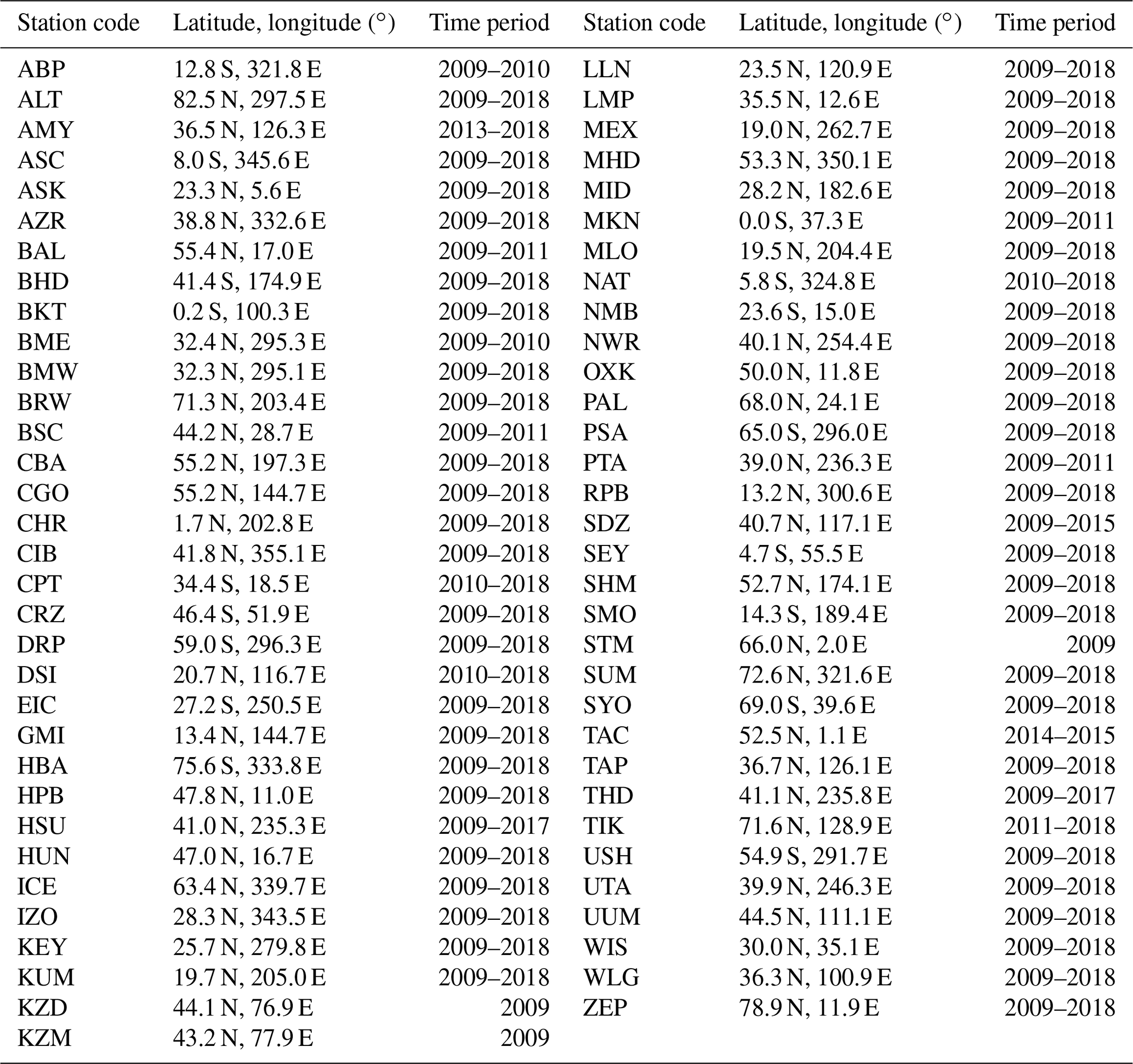
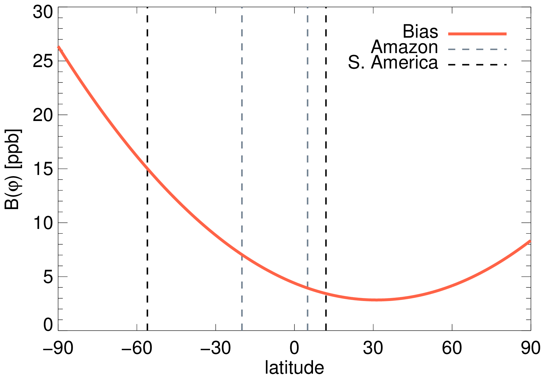
Figure A1Model–satellite bias function B(φ) (red line) varying with latitude, φ. This value is added to the simulated XCH4 to enable comparison with the GOSAT XCH4. See main text for details. Vertical grey and black dotted lines show the latitudinal extent of the Amazon basin and South America, respectively.
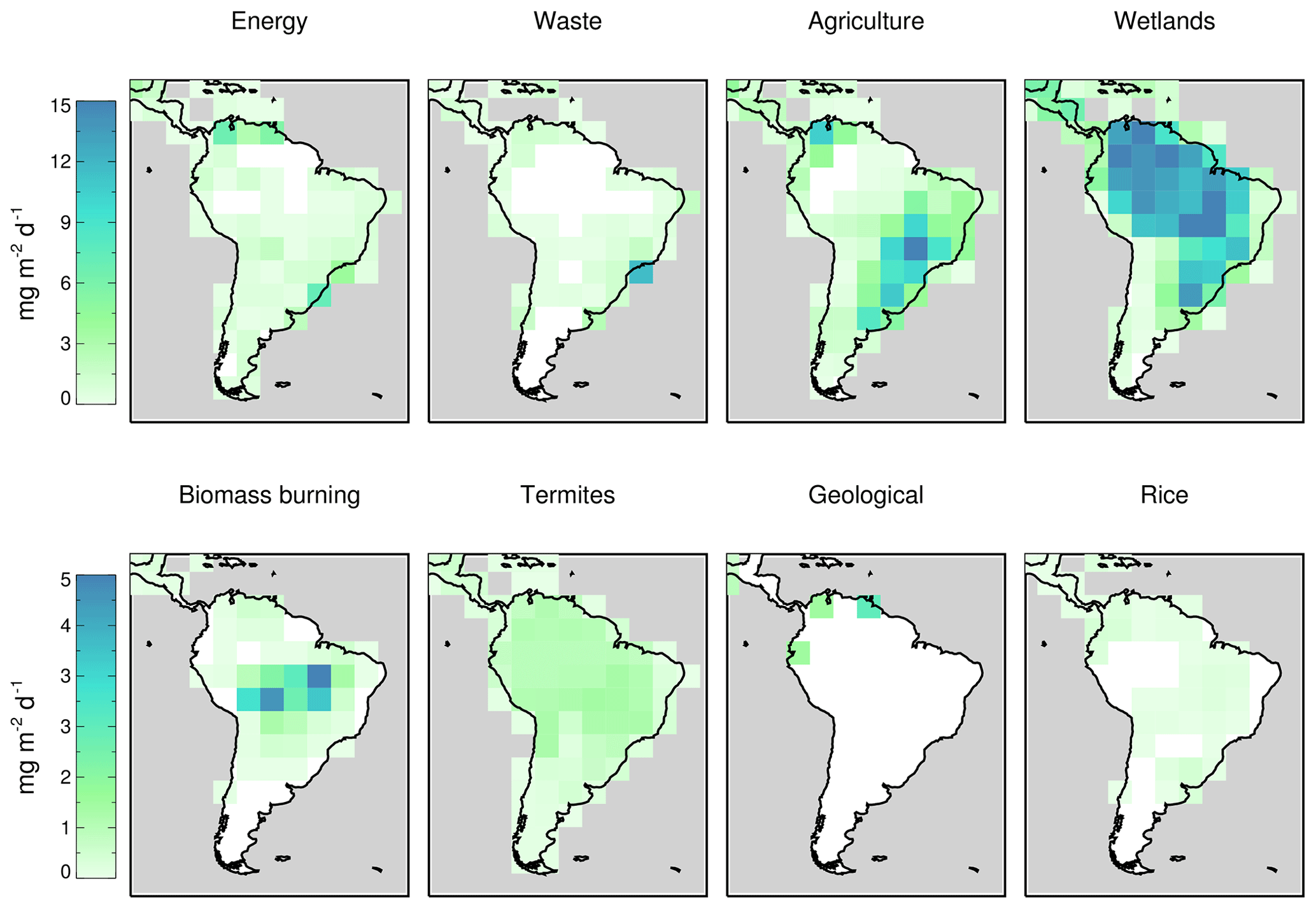
Figure A2A priori gridded sectoral South American CH4 emissions (mg m−2 d−1) for 2010. Note different colour scales for top and bottom rows. Description of sectoral emissions are in Sect. 2.2.2 of the main text. Here, the “Energy” sector refers to the energy industry, oil and gas production, and energy for buildings and transportation; “Waste” refers to solid waste disposal and waste water; “Agriculture” refers to enteric fermentation and manure management.
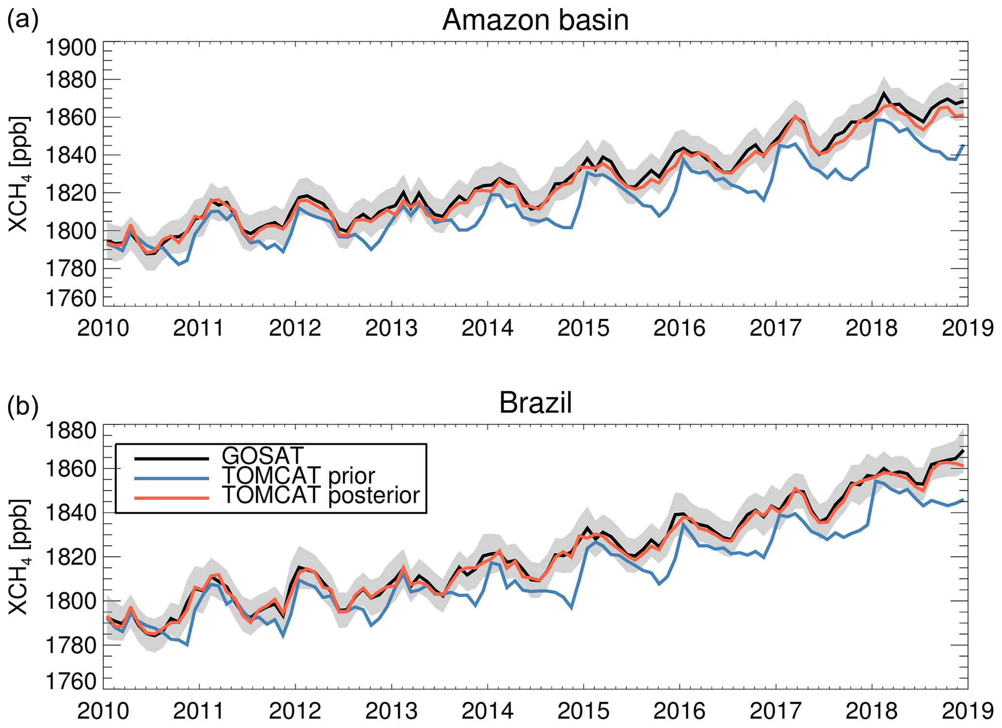
Figure A3Error-weighted monthly mean GOSAT XCH4 (black lines) over the Amazon basin (a) and Brazil (b). Also shown are the simulated mean prior (blue) and posterior (red) XCH4 values with GOSAT averaging kernels applied. Grey shading shows the monthly mean observation uncertainty within each region. It should be noted here that since simulations for each year were initiated using values from the previous year's posterior mean output for both the prior and the posterior initial atmospheric concentrations, the gradient of the blue line is artificially higher than it would be for a free-running simulation using the prior emissions only.
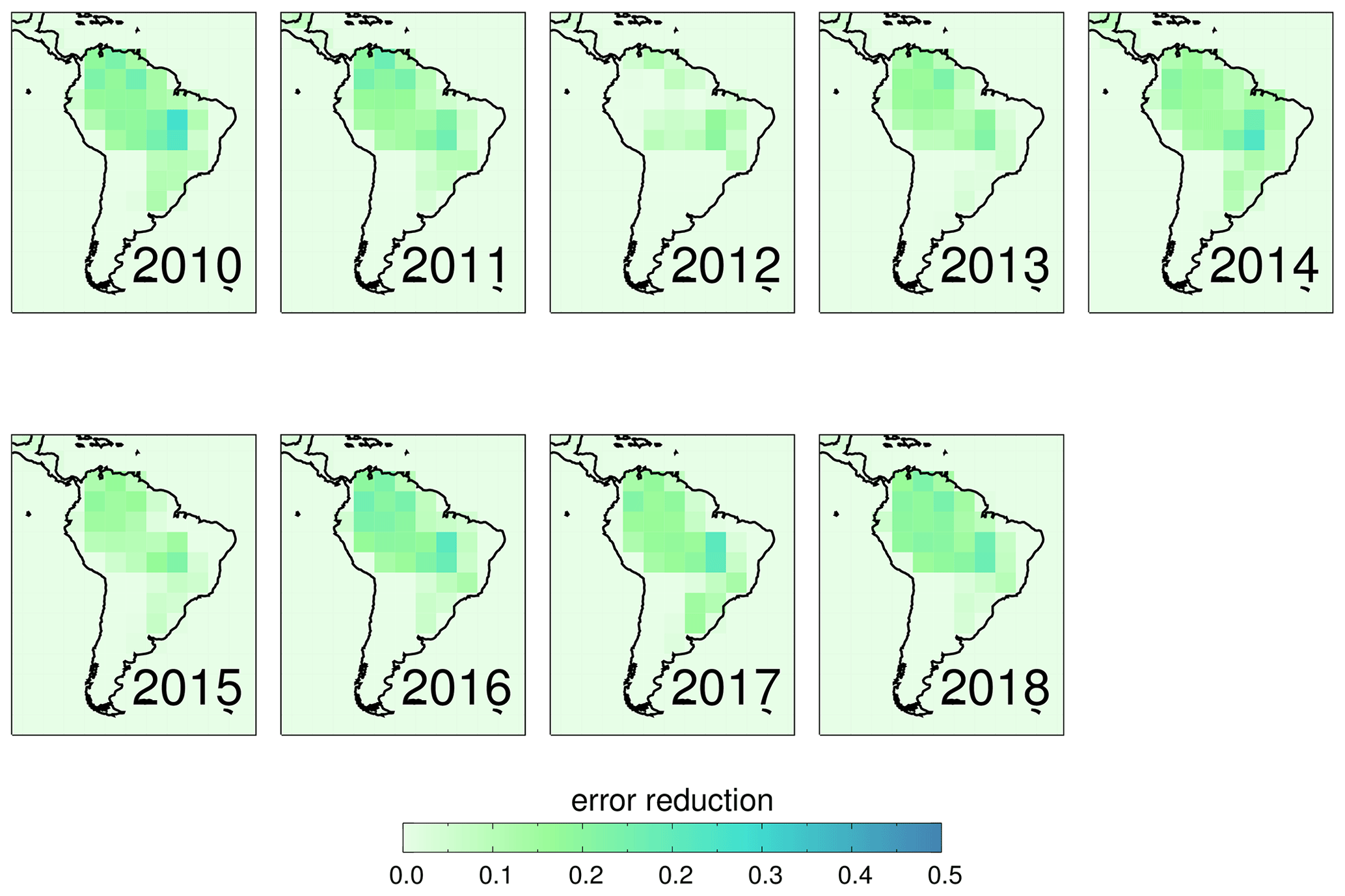
Figure A4Mean annual South American posterior error reduction after assimilation of GOSAT XCH4 and surface flask observations. Error reduction is defined as 1.-(σ_a/σ_b), where σ_a is the derived standard deviation of the a posteriori grid cell flux uncertainty and σb is the allocated a priori standard deviation of the grid cell flux uncertainty.

Figure A5Annual mean (posterior–prior) gridded total South American CH4 emissions (mg m−2 d−1) for each year covering the period 2010–2018.
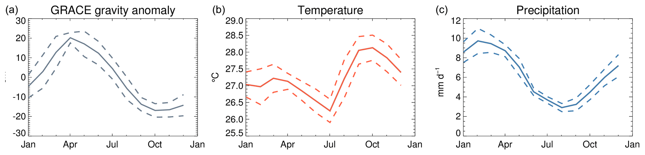
Figure A6Mean seasonal cycle of GRACE gravity anomaly (a, cm), temperature (b, ∘C) and precipitation (c, mm d−1) within the Amazon basin for 2010–2018. Dashed lines show 1 standard deviation from the mean values. Temperature is taken from the Global Historical Climatology Network (GHCN) gridded V2 product, whilst precipitation is from the Global Precipitation Climatology Project v2.3 combined precipitation dataset product. Both were provided by the NOAA/OAR/ESRL Physical Sciences Laboratory (PSL).
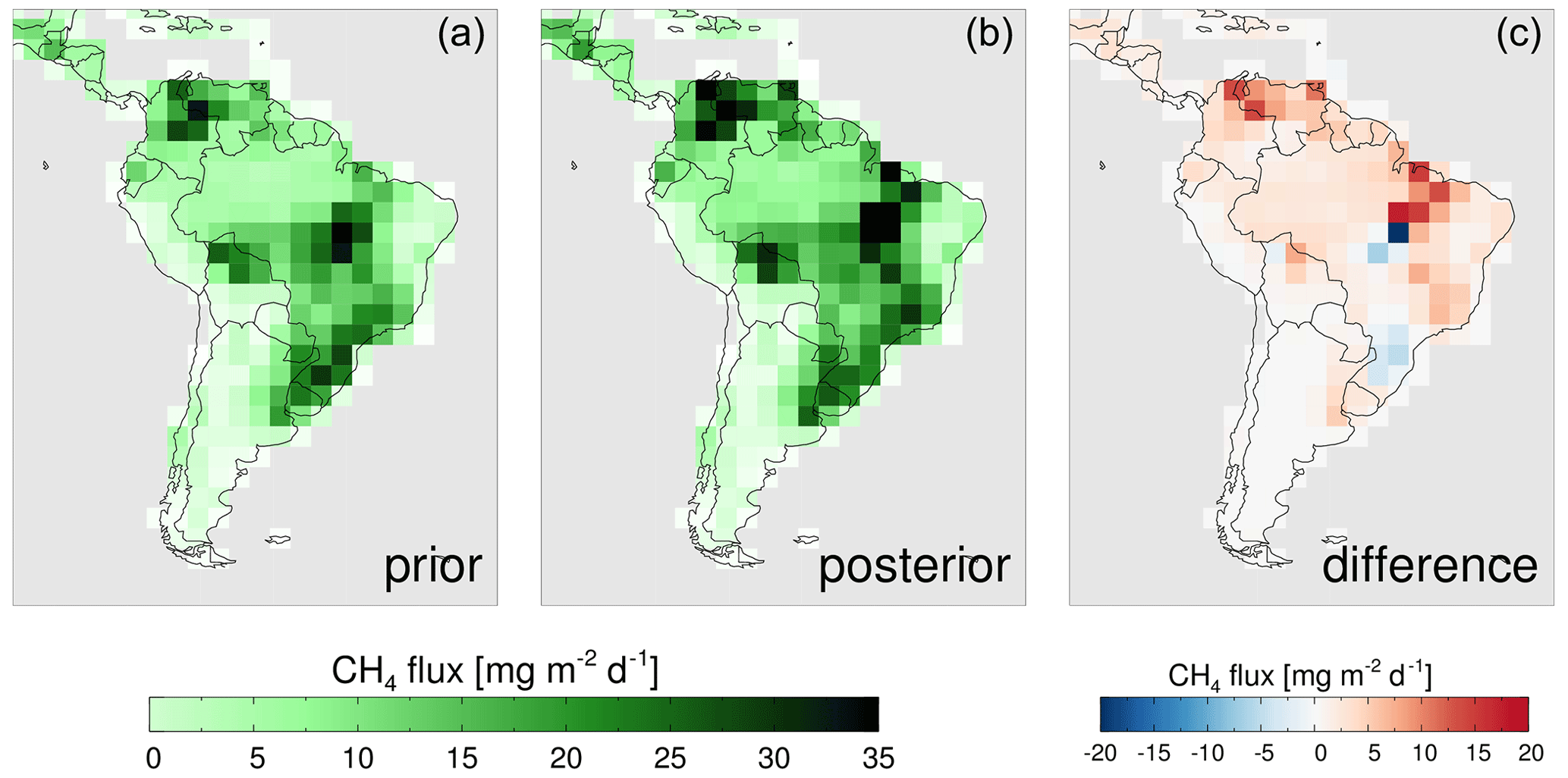
Figure A7Prior (a) and posterior (b) emissions of CH4 (mg m−2 d−1) for 2010 from an inversion carried out on the 2.8∘ degree model grid. (c) Posterior − prior emissions.
Our bottom-up (B-U) model calculates wetland CH4 emissions, in which the CH4 emissions in a grid cell, x, at time, t, are dependent on climatological factors as follows:
where F(tx) is the flux of CH4 in molec. cm−2 s−1, A(tx) is the wetland fraction, R(tx) is the heterotrophic respiration of carbon per unit area, T(tx) is the surface temperature in ∘C and q10 is the relative CH4:C ratio of respiration for a 10 ∘C change in temperature. Finally, s is a scaling factor. We use monthly mean values for each element of Eq. (2) and interpolate all parameters to the TOMCAT model grid for comparison with the inversion results.
We take R from the CASA-GFED v4.1 model (Randerson et al., 2015), which runs up to 2016, and gridded 2 m temperature from the Global Historical Climatology Network (GHCN) gridded V2 product provided by the NOAA/OAR/ESRL Physical Sciences Laboratory (PSL, https://psl.noaa.gov/, last access: 16 September 2019, Fan and Dool, 2008). We estimate A using a combination of two products. We take a climatology of wetland fraction w(x) from the JULES land surface model version that was used to produce the prior emissions used in the inversion (McNorton et al., 2016). We then use measurements of gravity anomalies made on the twin GRACE satellite mission, G(tx), as a proxy for variations in the soil moisture, as in (e.g.) Bloom et al. (2010) and Gloor et al. (2018). We then apply scaling factors a1 and a2 to give wetland fraction as follows:
This makes the assumption that anomalies in the gravity anomaly G(tx) are linearly related to wetland fraction anomalies, which may not be the case. The distributions and variations of the GRACE gravity anomalies and surface temperature are discussed in Sect. 4. We create an ensemble of B-U estimates for F, letting the scaling factors a1 and a2 and the temperature response function q10 vary within reasonable limits, and varying s appropriately so that each member gives the same mean total emissions over 2010–2017, equal to the mean posterior value produced by the inversion. We are interested only in the variations in time and space produced by the B-U model rather than the absolute value. We let q10 vary between 1 and 3, based on experimental bounds and previous bottom-up studies of methane emissions (Yvon-Durocher et al., 2014; Bloom et al., 2017); we let a1 vary between 0.8 and 1.2; and we let a2 vary in such a way that the overall wetland fraction does not vary by more than 20 %, depending on the value of a1. Since there is no data for 2017 given for the heterotrophic respiration, we use a climatology made up from the preceding 7 years applied to that year. We also create an “optimised” B-U model, in which we use a curve-fitting procedure (based on a gradient expansion algorithm) to choose values of s, a1, a2 and q10 which best fit, in least-squares terms, the results from the inversion for the monthly and spatial mean values over the whole Amazon, for all months within the wet season over 2010–2017. The optimised value of q10 was 2.47, which is within the range of plausible values discussed in Sect. 2.2.3, whilst the optimised values of a1 and a2 were 0.73 and 0.0015, respectively. For comparison to the B-U model, we consider only the posterior inversion NAT + AGR + BB emissions within the Amazon basin during the wet season, which we assume to be almost entirely from wetlands (Fig. A2). We therefore also only consider the B-U model output during the wet season.
We ran an inversion for 2010 at 2.8∘ horizontal grid resolution (Fig. A8) averaging the GOSAT XCH4 onto this model grid. We did not split the results into different source sectors, instead deriving total CH4 surface flux. Otherwise, the model set-up was identical to the 5.6∘ inversions of the main study. Many of the features of the posterior solution are identical to those of the coarser grid, with higher emissions from the region to the south and east of the Amazon River and a decrease in emissions from the south of Brazil, near the densely populated cities. However, there is no decrease in emissions to the west of the Amazon basin, as consistently seen when using the coarser model grid. Total derived emissions for Brazil and for the Amazon basin are similar when using the 2.8∘ and the 5.6∘ grids, however. We derive total posterior emissions for Brazil in 2010 of 49.9 Tg yr−1 using the coarser grid and 51.4 Tg yr−1 using the finer grid.
University of Leicester GOSAT Proxy XCH4 data can be accessed via the Centre for Environmental Data Analysis data repository at https://catalogue.ceda.ac.uk/uuid/f9154243fd8744bdaf2a59c39033e659 (ESA CCI GHG project team, 2018) or by contacting Rob Parker. Prior and posterior mean South American CH4 fluxes on the TOMCAT model grid (Wilson et al., 2021) are available from the data archive of the Centre for Environmental Data Analysis (CEDA, https://www.ceda.ac.uk/, last access: 2 June 2021, Wilson et al., 2021). The data DOI is https://doi.org/10.5285/88224a922439441fa6644b4564dcd90c.
CW, MPC and MG designed the methodology and wrote the manuscript. CW performed the analysis. RJP and HB provided the GOSAT data. JM and SAM provided TOMCAT model input. LVG, JBM and LSB provided the Amazon flight data. All authors contributed with analysis and text.
The authors declare that they have no conflict of interest.
Chris Wilson, Martyn P. Chipperfield, Robert J. Parker and Hartmut Boesch are funded via the UK National Centre for Earth Observation (NE/R016518/1 and NE/N018079/1). The work at Leeds was also supported by the NERC MOYA project (NE/N015657/1). We thank the Japanese Aerospace Exploration Agency, National Institute for Environmental Studies, and the Ministry of Environment for the GOSAT data and their continuous support as part of the Joint Research Agreement. This research used the ALICE High Performance Computing Facility at the University of Leicester for the GOSAT retrievals. Luciana V. Gatti, Luana S. Basso and John B. Miller are funded via the following grants: FAPESP (16/02018-2, 11/51841-0, 08/58120-3, 18/14006-4), NASA grants (11-CMS11-0025, NRMJ1000-17-00431), ERC Horizon 2020 (649087) and 7FP EU (283080). We thank Wuhu Feng for support for the TOMCAT model and Ross Bannister for advice regarding error covariance.
This research has been supported by National Environmental Research Council (NERC) UK grants through the National Centre for Earth Observation (NCEO, grant nos. NE/R016518/1 and NE/N018079/1) and the MOYA project (grant no. NE/N015657/1).
This paper was edited by Anja Schmidt and reviewed by Luke Western and two anonymous referees.
Adler, R. F., Sapiano, M. R. P., Huffman, G. J., Wang, J.-J., Gu, G., Bolvin, D., Chiu, L., Schneider, U., Becker, A., Nelkin, E., Xie, P., Ferraro, R., and Shin, D.-B.: The Global Precipitation Climatology Project (GPCP) Monthly Analysis (New Version 2.3) and a Review of 2017 Global Precipitation, Atmosphere, 9, 138, https://doi.org/10.3390/atmos9040138, 2018.
Anderson, D. C., Duncan, B. N., Fiore, A. M., Baublitz, C. B., Follette-Cook, M. B., Nicely, J. M., and Wolfe, G. M.: Spatial and temporal variability in the hydroxyl (OH) radical: understanding the role of large-scale climate features and their influence on OH through its dynamical and photochemical drivers, Atmos. Chem. Phys., 21, 6481–6508, https://doi.org/10.5194/acp-21-6481-2021, 2021.
Barichivich, J., Gloor, E., Peylin, P., Brienen, R. J. W., Schöngart, J., Espinoza, J. C., and Pattnayak, K. C.: Recent intensification of Amazon flooding extremes driven by strengthened Walker circulation, Sci. Adv., 4, EAAT8785, https://doi.org/10.1126/sciadv.aat8785, 2018.
Basso, L. S., Gatti, L. V., Gloor, M., Miller, J. B., Domingues, L. G., Correia, C. S. C., and Borges, V. F.: Seasonality and interannual variability of CH4 fluxes from the eastern Amazon Basin inferred from atmospheric mole fraction profiles, J. Geophys. Res.-Atmos., 121, 168–184, https://doi.org/10.1002/2015JD023874, 2016.
Bergamaschi, P., Frankenberg, C., Meirink, J. F., Krol, M., Villani, M. G., Houweling, S., Dentener, F., Dlugokencky, E. J., Miller, J. B., Gatti, L. V., Engel, A., and Levin, I.: Inverse modeling of global and regional CH4 emissions using SCIAMACHY satellite retrievals, J. Geophys. Res.-Atmos., 114, 2156–2202, https://doi.org/10.1029/2009JD012287, 2009.
Bloom, A. A., Palmer, P. I., Fraser, A., Reay, D. S., and Frankenberg, C.: Large-Scale Controls of Methanogenesis Inferred from Methane and Gravity Spaceborne Data, Science, 327, 322–325, https://doi.org/10.1126/science.1175176, 2010.
Bloom, A. A., Bowman, K. W., Lee, M., Turner, A. J., Schroeder, R., Worden, J. R., Weidner, R., McDonald, K. C., and Jacob, D. J.: A global wetland methane emissions and uncertainty dataset for atmospheric chemical transport models (WetCHARTs version 1.0), Geosci. Model Dev., 10, 2141–2156, https://doi.org/10.5194/gmd-10-2141-2017, 2017.
Bousserez, N., Henze, D. K., Perkins, A., Bowman, K. W., Lee, M., Liu, J., Deng, F., and Jones, D. B. A.: Improved analysis-error covariance matrix for high-dimensional variational inversions: application to source estimation using a 3D atmospheric transport model, Q. J. Roy. Meteor. Soc., 141, 1906–1921, https://doi.org/10.1002/qj.2495, 2015.
do Carmo, J. B., Keller, M., Dias, J. D., de Camargo, P. B., and Crill, P.: A source of methane from upland forests in the Brazilian Amazon, Geophys. Res. Lett., 33, https://doi.org/10.1029/2005GL025436, 2006.
Chandra, N., Patra, P. K., Bisht, J. S. H., Ito, A., Umezawa, T., Saigusa, N., Morimoto, S., Aoki, S., Janssens-Maenhout, G., Fujita, R., Takigawa, M., Watanabe, S., Saitoh, N., and Canadell, J. G.: Emissions from the Oil and Gas Sectors, Coal Mining and Ruminant Farming Drive Methane Growth over the Past Three Decades, J. Meteorol. Soc. Jpn., 99, 309–337, https://doi.org/10.2151/jmsj.2021-015, 2021.
Chevallier, F.: Impact of correlated observation errors on inverted CO2 surface fluxes from OCO measurements, Geophys. Res. Lett., 34, L24804, https://doi.org/10.1029/2007GL030463, 2007.
Chipperfield, M. P.: New version of the TOMCAT/SLIMCAT off-line chemical transport model: Intercomparison of stratospheric tracer experiments, Q. J. Roy. Meteor. Soc., 132, 1179–1203, https://doi.org/10.1256/qj.05.51, 2006.
Clark, D. B., Mercado, L. M., Sitch, S., Jones, C. D., Gedney, N., Best, M. J., Pryor, M., Rooney, G. G., Essery, R. L. H., Blyth, E., Boucher, O., Harding, R. J., Huntingford, C., and Cox, P. M.: The Joint UK Land Environment Simulator (JULES), model description – Part 2: Carbon fluxes and vegetation dynamics, Geosci. Model Dev., 4, 701–722, https://doi.org/10.5194/gmd-4-701-2011, 2011.
Crippa, M., Solazzo, E., Huang, G., Guizzardi, D., Koffi, E., Muntean, M., Schieberle, C., Friedrich, R., and Janssens-Maenhout, G.: High resolution temporal profiles in the Emissions Database for Global Atmospheric Research, Sci. Data, 7, 121, https://doi.org/10.1038/s41597-020-0462-2, 2020.
Dee, D. P., Uppala, S. M., Simmons, A. J., Berrisford, P., Poli, P., Kobayashi, S., Andrae, U., Balmaseda, M. A., Balsamo, G., Bauer, P., Bechtold, P., Beljaars, A. C. M., Berg, L. van de, Bidlot, J., Bormann, N., Delsol, C., Dragani, R., Fuentes, M., Geer, A. J., Haimberger, L., Healy, S. B., Hersbach, H., Hólm, E. V., Isaksen, L., Kållberg, P., Köhler, M., Matricardi, M., McNally, A. P., Monge-Sanz, B. M., Morcrette, J.-J., Park, B.-K., Peubey, C., Rosnay, P., de Tavolato, C., Thépaut, J.-N., and Vitart, F.: The ERA-Interim reanalysis: configuration and performance of the data assimilation system, Q. J. Roy. Meteor. Soc., 137, 553–597, https://doi.org/10.1002/qj.828, 2011.
Dlugokencky, E. J., Lang, P. M., Crotwell, A. M., Mund, J. W., Crotwell, M. J., and Thoning, K. W.: Atmospheric Methane Dry Air Mole Fractions from the NOAA ESRL Carbon Cycle Cooperative Global Air Sampling Network, Version: 2018-08-01, available at: ftp://aftp.cmdl.noaa.gov/data/trace_gases/ch4/flask/surface/ (last access: May 2021), 1983–2017, 2018.
ESA CCI GHG project team: ESA Greenhouse Gases Climate Change Initiative (GHG_cci): Column-averaged CH4 from GOSAT generated with the OCPR (UoL-PR) Proxy algorithm (CH4_GOS_OCPR), v7.0, available at: https://catalogue.ceda.ac.uk/uuid/f9154243fd8744bdaf2a59c39033e659 (last access: 2 June 2021), 2018.
Espinoza, J. C., Marengo, J. A., Ronchail, J., Carpio, J. M., Flores, L. N., and Guyot, J. L.: The extreme 2014 flood in south-western Amazon basin: the role of tropical-subtropical South Atlantic SST gradient, Environ. Res. Lett., 9, 124007, https://doi.org/10.1088/1748-9326/9/12/124007, 2014.
Fan, Y. and van den Dool, H.: A global monthly land surface air temperature analysis for 1948–present, 113, D01103, https://doi.org/10.1029/2007JD008470, 2008.
Feng, L., Palmer, P. I., Bösch, H., Parker, R. J., Webb, A. J., Correia, C. S. C., Deutscher, N. M., Domingues, L. G., Feist, D. G., Gatti, L. V., Gloor, E., Hase, F., Kivi, R., Liu, Y., Miller, J. B., Morino, I., Sussmann, R., Strong, K., Uchino, O., Wang, J., and Zahn, A.: Consistent regional fluxes of CH4 and CO2 inferred from GOSAT proxy XCH4 : XCO2 retrievals, 2010–2014, Atmos. Chem. Phys., 17, 4781–4797, https://doi.org/10.5194/acp-17-4781-2017, 2017.
Fraser, A., Palmer, P. I., Feng, L., Boesch, H., Cogan, A., Parker, R., Dlugokencky, E. J., Fraser, P. J., Krummel, P. B., Langenfelds, R. L., O'Doherty, S., Prinn, R. G., Steele, L. P., van der Schoot, M., and Weiss, R. F.: Estimating regional methane surface fluxes: the relative importance of surface and GOSAT mole fraction measurements, Atmos. Chem. Phys., 13, 5697–5713, https://doi.org/10.5194/acp-13-5697-2013, 2013.
Fujita, R., Morimoto, S., Maksyutov, S., Kim, H.-S., Arshinov, M., Brailsford, G., Aoki, S., and Nakazawa, T.: Global and Regional CH4 Emissions for 1995–2013 Derived From Atmospheric CH4, δ13C-CH4, and δD-CH4 Observations and a Chemical Transport Model, J. Geophys. Res.-Atmos., 125, e2020JD032903, https://doi.org/10.1029/2020JD032903, 2020.
Gatti, L. V., Gloor, M., Miller, J. B., Doughty, C. E., Malhi, Y., Domingues, L. G., Basso, L. S., Martinewski, A., Correia, C. S. C., Borges, V. F., Freitas, S., Braz, R., Anderson, L. O., Rocha, H., Grace, J., Phillips, O. L., and Lloyd, J.: Drought sensitivity of Amazonian carbon balance revealed by atmospheric measurements, Nature, 506, 76–80, https://doi.org/10.1038/nature12957, 2014.
Gloor, E., Wilson, C., Chipperfield, M. P., Chevallier, F., Buermann, W., Boesch, H., Parker, R., Somkuti, P., Gatti, L. V., Correia, C., Domingues, L. G., Peters, W., Miller, J., Deeter, M. N., and Sullivan, M. J. P.: Tropical land carbon cycle responses to 2015/16 El Niño as recorded by atmospheric greenhouse gas and remote sensing data, Philos. T. Roy. Soc. B, 373, 20170302, https://doi.org/10.1098/rstb.2017.0302, 2018.
Gumbricht, T., Roman-Cuesta, R. M., Verchot, L., Herold, M., Wittmann, F., Householder, E., Herold, N., and Murdiyarso, D.: An expert system model for mapping tropical wetlands and peatlands reveals South America as the largest contributor, Glob. Change Biol., 23, 3581–3599, https://doi.org/10.1111/gcb.13689, 2017.
Howarth, R. W.: Ideas and perspectives: is shale gas a major driver of recent increase in global atmospheric methane?, Biogeosciences, 16, 3033–3046, https://doi.org/10.5194/bg-16-3033-2019, 2019.
Huijnen, V., Williams, J., van Weele, M., van Noije, T., Krol, M., Dentener, F., Segers, A., Houweling, S., Peters, W., de Laat, J., Boersma, F., Bergamaschi, P., van Velthoven, P., Le Sager, P., Eskes, H., Alkemade, F., Scheele, R., Nédélec, P., and Pätz, H.-W.: The global chemistry transport model TM5: description and evaluation of the tropospheric chemistry version 3.0, Geosci. Model Dev., 3, 445–473, https://doi.org/10.5194/gmd-3-445-2010, 2010.
Jackson, R. B., Saunois, M., Bousquet, P., Canadell, J. G., Poulter, B., Stavert, A. R., Bergamaschi, P., Niwa, Y., Segers, A., and Tsuruta, A.: Increasing anthropogenic methane emissions arise equally from agricultural and fossil fuel sources, Environ. Res. Lett., 15, 071002, https://doi.org/10.1088/1748-9326/ab9ed2, 2020.
Janardanan, R., Maksyutov, S., Tsuruta, A., Wang, F., Tiwari, Y. K., Valsala, V., Ito, A., Yoshida, Y., Kaiser, J. W., Janssens-Maenhout, G., Arshinov, M., Sasakawa, M., Tohjima, Y., Worthy, D. E. J., Dlugokencky, E. J., Ramonet, M., Arduini, J., Lavric, J. V., Piacentino, S., Krummel, P. B., Langenfelds, R. L., Mammarella, I., and Matsunaga, T.: Country-Scale Analysis of Methane Emissions with a High-Resolution Inverse Model Using GOSAT and Surface Observations, Remote Sens., 12, 375, https://doi.org/10.3390/rs12030375, 2020.
Jiménez-Muñoz, J. C., Mattar, C., Barichivich, J., Santamaría-Artigas, A., Takahashi, K., Malhi, Y., Sobrino, J. A., and van der Schrier, G.: Record-breaking warming and extreme drought in the Amazon rainforest during the course of El Niño 2015–2016, Sci. Rep., 6, 33130, https://doi.org/10.1038/srep33130, 2016.
Kirschke, S., Bousquet, P., Ciais, P., Saunois, M., Canadell, J. G., Dlugokencky, E. J., Bergamaschi, P., Bergmann, D., Blake, D. R., Bruhwiler, L., Cameron-Smith, P., Castaldi, S., Chevallier, F., Feng, L., Fraser, A., Heimann, M., Hodson, E. L., Houweling, S., Josse, B., Fraser, P. J., Krummel, P. B., Lamarque, J.-F., Langenfelds, R. L., Le Quéré, C., Naik, V., O'Doherty, S., Palmer, P. I., Pison, I., Plummer, D., Poulter, B., Prinn, R. G., Rigby, M., Ringeval, B., Santini, M., Schmidt, M., Shindell, D. T., Simpson, I. J., Spahni, R., Steele, L. P., Strode, S. A., Sudo, K., Szopa, S., van der Werf, G. R., Voulgarakis, A., van Weele, M., Weiss, R. F., Williams, J. E., and Zeng, G.: Three decades of global methane sources and sinks, Nat. Geosci., 6, 813–823, https://doi.org/10.1038/ngeo1955, 2013.
Kuze, A., Suto, H., Nakajima, M., and Hamazaki, T.: Thermal and near infrared sensor for carbon observation Fourier-transform spectrometer on the Greenhouse Gases Observing Satellite for greenhouse gases monitoring, Appl. Opt., 48, 6716–6733, https://doi.org/10.1364/AO.48.006716, 2009.
Lan, X., Tans, P., Sweeney, C., Andrews, A., Dlugokencky, E., Schwietzke, S., Kofler, J., McKain, K., Thoning, K., Crotwell, M., Montzka, S., Miller, B. R., and Biraud, S. C.: Long-Term Measurements Show Little Evidence for Large Increases in Total U.S. Methane Emissions Over the Past Decade, Geophys. Res. Lett., 46, 4991–4999, https://doi.org/10.1029/2018GL081731, 2019.
Lewis, S. L., Brando, P. M., Phillips, O. L., van der Heijden, G. M. F., and Nepstad, D.: The 2010 Amazon Drought, Science, 331, 554–554, https://doi.org/10.1126/science.1200807, 2011.
McNorton, J., Chipperfield, M. P., Gloor, M., Wilson, C., Feng, W., Hayman, G. D., Rigby, M., Krummel, P. B., O'Doherty, S., Prinn, R. G., Weiss, R. F., Young, D., Dlugokencky, E., and Montzka, S. A.: Role of OH variability in the stalling of the global atmospheric CH4 growth rate from 1999 to 2006, Atmos. Chem. Phys., 16, 7943–7956, https://doi.org/10.5194/acp-16-7943-2016, 2016a.
McNorton, J., Gloor, E., Wilson, C., Hayman, G. D., Gedney, N., Comyn-Platt, E., Marthews, T., Parker, R. J., Boesch, H., and Chipperfield, M. P.: Role of regional wetland emissions in atmospheric methane variability, Geophys. Res. Lett., 43, 11433–11444, https://doi.org/10.1002/2016GL070649, 2016b.
McNorton, J., Wilson, C., Gloor, M., Parker, R. J., Boesch, H., Feng, W., Hossaini, R., and Chipperfield, M. P.: Attribution of recent increases in atmospheric methane through 3-D inverse modelling, Atmos. Chem. Phys., 18, 18149–18168, https://doi.org/10.5194/acp-18-18149-2018, 2018.
Meirink, J. F., Bergamaschi, P., and Krol, M. C.: Four-dimensional variational data assimilation for inverse modelling of atmospheric methane emissions: method and comparison with synthesis inversion, Atmos. Chem. Phys., 8, 6341–6353, https://doi.org/10.5194/acp-8-6341-2008, 2008.
Melack, J. M., Hess, L. L., Gastil, M., Forsberg, B. R., Hamilton, S. K., Lima, I. B. T., and Novo, E. M. L. M.: Regionalization of methane emissions in the Amazon Basin with microwave remote sensing, Science, 10, 530–544, https://doi.org/10.1111/j.1365-2486.2004.00763.x, 2004.
Melton, J. R., Wania, R., Hodson, E. L., Poulter, B., Ringeval, B., Spahni, R., Bohn, T., Avis, C. A., Beerling, D. J., Chen, G., Eliseev, A. V., Denisov, S. N., Hopcroft, P. O., Lettenmaier, D. P., Riley, W. J., Singarayer, J. S., Subin, Z. M., Tian, H., Zürcher, S., Brovkin, V., van Bodegom, P. M., Kleinen, T., Yu, Z. C., and Kaplan, J. O.: Present state of global wetland extent and wetland methane modelling: conclusions from a model inter-comparison project (WETCHIMP), Biogeosciences, 10, 753–788, https://doi.org/10.5194/bg-10-753-2013, 2013.
Miller, J. B., Gatti, L. V., d'Amelio, M. T. S., Crotwell, A. M., Dlugokencky, E. J., Bakwin, P., Artaxo, P., and Tans, P. P.: Airborne measurements indicate large methane emissions from the eastern Amazon basin, Geophys. Res. Lett., 34, L10809, https://doi.org/10.1029/2006GL029213, 2007.
Miller, S. M., Michalak, A. M., Detmers, R. G., Hasekamp, O. P., Bruhwiler, L. M. P., and Schwietzke, S.: China's coal mine methane regulations have not curbed growing emissions, Nat. Commun., 10, 303, https://doi.org/10.1038/s41467-018-07891-7, 2019.
Monks, S. A., Arnold, S. R., Hollaway, M. J., Pope, R. J., Wilson, C., Feng, W., Emmerson, K. M., Kerridge, B. J., Latter, B. L., Miles, G. M., Siddans, R., and Chipperfield, M. P.: The TOMCAT global chemical transport model v1.6: description of chemical mechanism and model evaluation, Geosci. Model Dev., 10, 3025–3057, https://doi.org/10.5194/gmd-10-3025-2017, 2017.
Monks, S. A., Wilson, C., Emmons, L. K., Hannigan, J. W., Helmig, D., Blake, N. J., and Blake, D. R.: Using an Inverse Model to Reconcile Differences in Simulated and Observed Global Ethane Concentrations and Trends Between 2008 and 2014, J. Geophys. Res.-Atmos., 123, 11262–11282, https://doi.org/10.1029/2017JD028112, 2018.
Montzka, S. A., Krol, M., Dlugokencky, E., Hall, B., Jöckel, P., and Lelieveld, J.: Small Interannual Variability of Global Atmospheric Hydroxyl, Science, 331, 67–69, https://doi.org/10.1126/science.119740, 2011.
Murguia-Flores, F., Arndt, S., Ganesan, A. L., Murray-Tortarolo, G., and Hornibrook, E. R. C.: Soil Methanotrophy Model (MeMo v1.0): a process-based model to quantify global uptake of atmospheric methane by soil, Geosci. Model Dev., 11, 2009–2032, https://doi.org/10.5194/gmd-11-2009-2018, 2018.
Myhre, G., Shindell, D., Bréon, F.-M., Collins, W., Fuglestvedt, J., Huang, J., Koch, D., Lamarque, J.-F., Lee, D., Mendoza, B., Nakajima, T., Robock, A., Stephens, G., Zhang, H., Aamaas, B., Boucher, O., Dalsøren, S. B., Daniel, J. S., Forster, P., Granier, C., Haigh, J., Hodnebrog, Ø., Kaplan, J. O., Marston, G., Nielsen, C. J., O'Neill, B. C., Peters, G. P., Pongratz, J., Ramaswamy, V., Roth, R., Rotstayn, L., Smith, S. J., Stevenson, D., Vernier, J.-P., Wild, O., Young, P., Jacob, D., Ravishankara, A. R., and Shine, K.: Anthropogenic and Natural Radiative Forcing, Climate Change 2013: The Physical Science Basis, Contribution of Working Group I to the Fifth Assessment Report of the Intergovernmental Panel on Climate Change, edited by: Stocker, T. F., Qin, D., Plattner, G.-K., Tignor, M., Allen, S. K., Boschung, J., Nauels, A., Xia, Y., Bex, V., and Midgley, P. M., Cambridge University Press, Cambridge, United Kingdom and New York, NY, USA, 2013.
Naus, S., Montzka, S. A., Patra, P. K., and Krol, M. C.: A three-dimensional-model inversion of methyl chloroform to constrain the atmospheric oxidative capacity, Atmos. Chem. Phys., 21, 4809–4824, https://doi.org/10.5194/acp-21-4809-2021, 2021.
Nisbet, E. G., Dlugokencky, E. J., Manning, M. R., Lowry, D., Fisher, R. E., France, J. L., Michel, S. E., Miller, J. B., White, J. W. C., Vaughn, B., Bousquet, P., Pyle, J. A., Warwick, N. J., Cain, M., Brownlow, R., Zazzeri, G., Lanoisellé, M., Manning, A. C., Gloor, E., Worthy, D. E. J., Brunke, E.-G., Labuschagne, C., Wolff, E. W., and Ganesan, A. L.: Rising atmospheric methane: 2007–2014 growth and isotopic shift, Global Biogeochem. Cy., 30, 1356–1370, https://doi.org/10.1002/2016GB005406, 2016.
Nisbet, E. G., Manning, M. R., Dlugokencky, E. J., Fisher, R. E., Lowry, D., Michel, S. E., Myhre, C. L., Platt, S. M., Allen, G., Bousquet, P., Brownlow, R., Cain, M., France, J. L., Hermansen, O., Hossaini, R., Jones, A. E., Levin, I., Manning, A. C., Myhre, G., Pyle, J. A., Vaughn, B. H., Warwick, N. J., and White, J. W. C.: Very Strong Atmospheric Methane Growth in the 4 Years 2014–2017: Implications for the Paris Agreement, Global Biogeochem. Cy., 33, 318–342, https://doi.org/10.1029/2018GB006009, 2019.
Nocedal, J.: Updating quasi-Newton matrices with limited storage, Math. Comp., 35, 773–782, https://doi.org/10.1090/S0025-5718-1980-0572855-7, 1980.
Olivier, J. G., Peters, J. A., and Janssens-Maenhout, G.: Trends in Global CO2 Emissions 2012 Report, 40 pp., 2012.
Pangala, S. R., Enrich-Prast, A., Basso, L. S., Peixoto, R. B., Bastviken, D., Hornibrook, E. R. C., Gatti, L. V., Marotta, H., Calazans, L. S. B., Sakuragui, C. M., Bastos, W. R., Malm, O., Gloor, E., Miller, J. B., and Gauci, V.: Large emissions from floodplain trees close the Amazon methane budget, Nature, 552, 230–234, https://doi.org/10.1038/nature24639, 2017.
Parker, R., Boesch, H., Cogan, A., Fraser, A., Feng, L., Palmer, P. I., Messerschmidt, J., Deutscher, N., Griffith, D. W. T., Notholt, J., Wennberg, P. O., and Wunch, D.: Methane observations from the Greenhouse Gases Observing SATellite: Comparison to ground-based TCCON data and model calculations, Geophys. Res. Lett., 38, L15807, https://doi.org/10.1029/2011GL047871, 2011.
Parker, R. J., Boesch, H., McNorton, J., Comyn-Platt, E., Gloor, M., Wilson, C., Chipperfield, M. P., Hayman, G. D., and Bloom, A. A.: Evaluating year-to-year anomalies in tropical wetland methane emissions using satellite CH4 observations, Remote Sens. Environ., 211, 261–275, https://doi.org/10.1016/j.rse.2018.02.011, 2018.
Parker, R. J., Webb, A., Boesch, H., Somkuti, P., Barrio Guillo, R., Di Noia, A., Kalaitzi, N., Anand, J. S., Bergamaschi, P., Chevallier, F., Palmer, P. I., Feng, L., Deutscher, N. M., Feist, D. G., Griffith, D. W. T., Hase, F., Kivi, R., Morino, I., Notholt, J., Oh, Y.-S., Ohyama, H., Petri, C., Pollard, D. F., Roehl, C., Sha, M. K., Shiomi, K., Strong, K., Sussmann, R., Té, Y., Velazco, V. A., Warneke, T., Wennberg, P. O., and Wunch, D.: A decade of GOSAT Proxy satellite CH4 observations, Earth Syst. Sci. Data, 12, 3383–3412, https://doi.org/10.5194/essd-12-3383-2020, 2020a.
Parker, R. J., Wilson, C., Bloom, A. A., Comyn-Platt, E., Hayman, G., McNorton, J., Boesch, H., and Chipperfield, M. P.: Exploring constraints on a wetland methane emission ensemble (WetCHARTs) using GOSAT observations, Biogeosciences, 17, 5669–5691, https://doi.org/10.5194/bg-17-5669-2020, 2020b.
Patra, P. K., Houweling, S., Krol, M., Bousquet, P., Belikov, D., Bergmann, D., Bian, H., Cameron-Smith, P., Chipperfield, M. P., Corbin, K., Fortems-Cheiney, A., Fraser, A., Gloor, E., Hess, P., Ito, A., Kawa, S. R., Law, R. M., Loh, Z., Maksyutov, S., Meng, L., Palmer, P. I., Prinn, R. G., Rigby, M., Saito, R., and Wilson, C.: TransCom model simulations of CH4 and related species: linking transport, surface flux and chemical loss with CH4 variability in the troposphere and lower stratosphere, Atmos. Chem. Phys., 11, 12813–12837, https://doi.org/10.5194/acp-11-12813-2011, 2011.
Patra, P. K., Krol, M. C., Prinn, R. G., Takigawa, M., Mühle, J., Montzka, S. A., Lal, S., Yamashita, Y., Naus, S., Chandra, N., Weiss, R. F., Krummel, P. B., Fraser, P. J., O'Doherty, S., and Elkins, J. W.: Methyl Chloroform Continues to Constrain the Hydroxyl (OH) Variability in the Troposphere, J. Geophys. Res.-Atmos., 126, e2020JD033862, https://doi.org/10.1029/2020JD033862, 2021.
Poulter, B., Aragão, L., Heyder, U., Gumpenberger, M., Heinke, J., Langerwisch, F., Rammig, A., Thonicke, K., and Cramer, W.: Net biome production of the Amazon Basin in the 21st century, Glob. Change Biol., 16, 2062–2075, https://doi.org/10.1111/j.1365-2486.2009.02064.x, 2010.
Prather, M. J., Holmes, C. D., and Hsu, J.: Reactive greenhouse gas scenarios: Systematic exploration of uncertainties and the role of atmospheric chemistry, Geophys. Res. Lett., 39, L09803, https://doi.org/10.1029/2012GL051440, 2012.
Randerson, J. T., Van Der Werf, G. R., Giglio, L., Collatz, G. J., and Kasibhatla, P. S.: Global Fire Emissions Database, Version 4.1 (GFEDv4), https://doi.org/10.3334/ORNLDAAC/1293, 2015.
Rigby, M., Montzka, S. A., Prinn, R. G., White, J. W. C., Young, D., O'Doherty, S., Lunt, M. F., Ganesan, A. L., Manning, A. J., Simmonds, P. G., Salameh, P. K., Harth, C. M., Mühle, J., Weiss, R. F., Fraser, P. J., Steele, L. P., Krummel, P. B., McCulloch, A., and Park, S.: Role of atmospheric oxidation in recent methane growth, P. Natl. Acad. Sci. USA, 114, 5373–5377, https://doi.org/10.1073/pnas.1616426114, 2017.
Ringeval, B., Houweling, S., van Bodegom, P. M., Spahni, R., van Beek, R., Joos, F., and Röckmann, T.: Methane emissions from floodplains in the Amazon Basin: challenges in developing a process-based model for global applications, Biogeosciences, 11, 1519–1558, https://doi.org/10.5194/bg-11-1519-2014, 2014.
Rowlinson, M. J., Rap, A., Arnold, S. R., Pope, R. J., Chipperfield, M. P., McNorton, J., Forster, P., Gordon, H., Pringle, K. J., Feng, W., Kerridge, B. J., Latter, B. L., and Siddans, R.: Impact of El Niño–Southern Oscillation on the interannual variability of methane and tropospheric ozone, Atmos. Chem. Phys., 19, 8669–8686, https://doi.org/10.5194/acp-19-8669-2019, 2019.
Rubino, M., Etheridge, D. M., Thornton, D. P., Howden, R., Allison, C. E., Francey, R. J., Langenfelds, R. L., Steele, L. P., Trudinger, C. M., Spencer, D. A., Curran, M. A. J., van Ommen, T. D., and Smith, A. M.: Revised records of atmospheric trace gases CO2, CH4, N2O, and δ13C-CO2 over the last 2000 years from Law Dome, Antarctica, Earth Syst. Sci. Data, 11, 473–492, https://doi.org/10.5194/essd-11-473-2019, 2019.
Saunois, M., Bousquet, P., Poulter, B., Peregon, A., Ciais, P., Canadell, J. G., Dlugokencky, E. J., Etiope, G., Bastviken, D., Houweling, S., Janssens-Maenhout, G., Tubiello, F. N., Castaldi, S., Jackson, R. B., Alexe, M., Arora, V. K., Beerling, D. J., Bergamaschi, P., Blake, D. R., Brailsford, G., Brovkin, V., Bruhwiler, L., Crevoisier, C., Crill, P., Covey, K., Curry, C., Frankenberg, C., Gedney, N., Höglund-Isaksson, L., Ishizawa, M., Ito, A., Joos, F., Kim, H.-S., Kleinen, T., Krummel, P., Lamarque, J.-F., Langenfelds, R., Locatelli, R., Machida, T., Maksyutov, S., McDonald, K. C., Marshall, J., Melton, J. R., Morino, I., Naik, V., O'Doherty, S., Parmentier, F.-J. W., Patra, P. K., Peng, C., Peng, S., Peters, G. P., Pison, I., Prigent, C., Prinn, R., Ramonet, M., Riley, W. J., Saito, M., Santini, M., Schroeder, R., Simpson, I. J., Spahni, R., Steele, P., Takizawa, A., Thornton, B. F., Tian, H., Tohjima, Y., Viovy, N., Voulgarakis, A., van Weele, M., van der Werf, G. R., Weiss, R., Wiedinmyer, C., Wilton, D. J., Wiltshire, A., Worthy, D., Wunch, D., Xu, X., Yoshida, Y., Zhang, B., Zhang, Z., and Zhu, Q.: The global methane budget 2000–2012, Earth Syst. Sci. Data, 8, 697–751, https://doi.org/10.5194/essd-8-697-2016, 2016.
Saunois, M., Stavert, A. R., Poulter, B., Bousquet, P., Canadell, J. G., Jackson, R. B., Raymond, P. A., Dlugokencky, E. J., Houweling, S., Patra, P. K., Ciais, P., Arora, V. K., Bastviken, D., Bergamaschi, P., Blake, D. R., Brailsford, G., Bruhwiler, L., Carlson, K. M., Carrol, M., Castaldi, S., Chandra, N., Crevoisier, C., Crill, P. M., Covey, K., Curry, C. L., Etiope, G., Frankenberg, C., Gedney, N., Hegglin, M. I., Höglund-Isaksson, L., Hugelius, G., Ishizawa, M., Ito, A., Janssens-Maenhout, G., Jensen, K. M., Joos, F., Kleinen, T., Krummel, P. B., Langenfelds, R. L., Laruelle, G. G., Liu, L., Machida, T., Maksyutov, S., McDonald, K. C., McNorton, J., Miller, P. A., Melton, J. R., Morino, I., Müller, J., Murguia-Flores, F., Naik, V., Niwa, Y., Noce, S., O'Doherty, S., Parker, R. J., Peng, C., Peng, S., Peters, G. P., Prigent, C., Prinn, R., Ramonet, M., Regnier, P., Riley, W. J., Rosentreter, J. A., Segers, A., Simpson, I. J., Shi, H., Smith, S. J., Steele, L. P., Thornton, B. F., Tian, H., Tohjima, Y., Tubiello, F. N., Tsuruta, A., Viovy, N., Voulgarakis, A., Weber, T. S., van Weele, M., van der Werf, G. R., Weiss, R. F., Worthy, D., Wunch, D., Yin, Y., Yoshida, Y., Zhang, W., Zhang, Z., Zhao, Y., Zheng, B., Zhu, Q., Zhu, Q., and Zhuang, Q.: The Global Methane Budget 2000–2017, Earth Syst. Sci. Data, 12, 1561–1623, https://doi.org/10.5194/essd-12-1561-2020, 2020.
Schaefer, H.: On the Causes and Consequences of Recent Trends in Atmospheric Methane, Curr. Clim. Change Rep., 5, 259–274, https://doi.org/10.1007/s40641-019-00140-z, 2019.
Schaefer, H., Fletcher, S. E. M., Veidt, C., Lassey, K. R., Brailsford, G. W., Bromley, T. M., Dlugokencky, E. J., Michel, S. E., Miller, J. B., Levin, I., Lowe, D. C., Martin, R. J., Vaughn, B. H., and White, J. W. C.: A 21st-century shift from fossil-fuel to biogenic methane emissions indicated by 13CH4, Science, 352, 80–84, https://doi.org/10.1126/science.aad2705, 2016.
Shindell, D., Kuylenstierna, J. C. I., Vignati, E., Dingenen, R. van, Amann, M., Klimont, Z., Anenberg, S. C., Muller, N., Janssens-Maenhout, G., Raes, F., Schwartz, J., Faluvegi, G., Pozzoli, L., Kupiainen, K., Höglund-Isaksson, L., Emberson, L., Streets, D., Ramanathan, V., Hicks, K., Oanh, N. T. K., Milly, G., Williams, M., Demkine, V., and Fowler, D.: Simultaneously Mitigating Near-Term Climate Change and Improving Human Health and Food Security, Science, 335, 183–189, https://doi.org/10.1126/science.1210026, 2012.
Silva Junior, C. H. L., Anderson, L. O., Silva, A. L., Almeida, C. T., Dalagnol, R., Pletsch, M. A. J. S., Penha, T. V., Paloschi, R. A., and Aragão, L. E. O. C.: Fire Responses to the 2010 and 2015/2016 Amazonian Droughts, Front. Earth Sci., 7, 97, https://doi.org/10.3389/feart.2019.00097, 2019.
Spivakovsky, C. M., Logan, J. A., Montzka, S. A., Balkanski, Y. J., Foreman-Fowler, M., Jones, D. B. A., Horowitz, L. W., Fusco, A. C., Brenninkmeijer, C. A. M., Prather, M. J., Wofsy, S. C., and McElroy, M. B.: Three-dimensional climatological distribution of tropospheric OH: Update and evaluation, J. Geophys. Res.-Atmos., 105, 8931–8980, https://doi.org/10.1029/1999JD901006, 2000.
Thompson, R. L., Nisbet, E. G., Pisso, I., Stohl, A., Blake, D., Dlugokencky, E. J., Helmig, D., and White, J. W. C.: Variability in Atmospheric Methane From Fossil Fuel and Microbial Sources Over the Last Three Decades, Geophys. Res. Lett., 45, 11499—11508, https://doi.org/10.1029/2018GL078127, 2018.
Thompson, R. L., Lassaletta, L., Patra, P. K., Wilson, C., Wells, K. C., Gressent, A., Koffi, E. N., Chipperfield, M. P., Winiwarter, W., Davidson, E. A., Tian, H., and Canadell, J. G.: Acceleration of global N2O emissions seen from two decades of atmospheric inversion, Science, 9, 993–998, https://doi.org/10.1038/s41558-019-0613-7, 2019.
Tian, H., Xu, R., Canadell, J. G., Thompson, R. L., Winiwarter, W., Suntharalingam, P., Davidson, E. A., Ciais, P., Jackson, R. B., Janssens-Maenhout, G., Prather, M. J., Regnier, P., Pan, N., Pan, S., Peters, G. P., Shi, H., Tubiello, F. N., Zaehle, S., Zhou, F., Arneth, A., Battaglia, G., Berthet, S., Bopp, L., Bouwman, A. F., Buitenhuis, E. T., Chang, J., Chipperfield, M. P., Dangal, S. R. S., Dlugokencky, E., Elkins, J. W., Eyre, B. D., Fu, B., Hall, B., Ito, A., Joos, F., Krummel, P. B., Landolfi, A., Laruelle, G. G., Lauerwald, R., Li, W., Lienert, S., Maavara, T., MacLeod, M., Millet, D. B., Olin, S., Patra, P. K., Prinn, R. G., Raymond, P. A., Ruiz, D. J., van der Werf, G. R., Vuichard, N., Wang, J., Weiss, R. F., Wells, K. C., Wilson, C., Yang, J., and Yao, Y.: A comprehensive quantification of global nitrous oxide sources and sinks, Science, 586, 248–256, https://doi.org/10.1038/s41586-020-2780-0, 2020.
Tunnicliffe, R. L., Ganesan, A. L., Parker, R. J., Boesch, H., Gedney, N., Poulter, B., Zhang, Z., Lavrič, J. V., Walter, D., Rigby, M., Henne, S., Young, D., and O'Doherty, S.: Quantifying sources of Brazil's CH4 emissions between 2010 and 2018 from satellite data, Atmos. Chem. Phys., 20, 13041–13067, https://doi.org/10.5194/acp-20-13041-2020, 2020.
Turner, A. J., Frankenberg, C., Wennberg, P. O., and Jacob, D. J.: Ambiguity in the causes for decadal trends in atmospheric methane and hydroxyl, P. Natl. Acad. Sci. USA, 114, 5367–5372, https://doi.org/10.1073/pnas.1616020114, 2017.
Webb, A. J., Bösch, H., Parker, R. J., Gatti, L. V., Gloor, E., Palmer, P. I., Basso, L. S., Chipperfield, M. P., Correia, C. S. C., Domingues, L. G., Feng, L., Gonzi, S., Miller, J. B., Warneke, T., and Wilson, C.: CH4 concentrations over the Amazon from GOSAT consistent with in situ vertical profile data, Science, 121, 11006–11020, https://doi.org/10.1002/2016JD025263, 2016.
van der Werf, G. R., Randerson, J. T., Giglio, L., van Leeuwen, T. T., Chen, Y., Rogers, B. M., Mu, M., van Marle, M. J. E., Morton, D. C., Collatz, G. J., Yokelson, R. J., and Kasibhatla, P. S.: Global fire emissions estimates during 1997–2016, Earth Syst. Sci. Data, 9, 697–720, https://doi.org/10.5194/essd-9-697-2017, 2017.
Wilson, C., Chipperfield, M. P., Gloor, M., and Chevallier, F.: Development of a variational flux inversion system (INVICAT v1.0) using the TOMCAT chemical transport model, Geosci. Model Dev., 7, 2485–2500, https://doi.org/10.5194/gmd-7-2485-2014, 2014.
Wilson, C., Gloor, M., Gatti, L. V., Miller, J. B., Monks, S. A., McNorton, J., Bloom, A. A., Basso, L. S., and Chipperfield, M. P.: Contribution of regional sources to atmospheric methane over the Amazon Basin in 2010 and 2011, Global Biogeochem. Cy., 30, 400–420, https://doi.org/10.1002/2015GB005300, 2016.
Wilson, C., Chipperfield, M., Gloor, M., Parker, R., and Boesch, H.: Posterior South American monthly mean surface flux of methane (2010–2018) produced using the INVICAT 4D-Var inverse model, Centre for Environmental Data Analysis, 17 February 2021, https://doi.org/10.5285/88224a922439441fa6644b4564dcd90c, last access: May 2021.
Worden, J. R., Bloom, A. A., Pandey, S., Jiang, Z., Worden, H. M., Walker, T. W., Houweling, S., and Röckmann, T.: Reduced biomass burning emissions reconcile conflicting estimates of the post-2006 atmospheric methane budget, Nat. Commun., 8, 2227, https://doi.org/10.1038/s41467-017-02246-0, 2017.
Wunch, D., Toon, G. C., Blavier, J.-F. L., Washenfelder, R. A., Notholt, J., Connor, B. J., Griffith, D. W. T., Sherlock, V., and Wennberg, P. O.: The Total Carbon Column Observing Network, Philos. T. Roy. Soc. A, 369, 2087–2112, https://doi.org/10.1098/rsta.2010.0240, 2011.
Yan, X., Akiyama, H., Yagi, K., and Akimoto, H.: Global estimations of the inventory and mitigation potential of methane emissions from rice cultivation conducted using the 2006 Intergovernmental Panel on Climate Change Guidelines, Global Biogeochem., Cy., 23, GB2002, https://doi.org/10.1029/2008GB003299, 2009.
Yin, Y., Chevallier, F., Ciais, P., Bousquet, P., Saunois, M., Zheng, B., Worden, J., Bloom, A. A., Parker, R., Jacob, D., Dlugokencky, E. J., and Frankenberg, C.: Accelerating methane growth rate from 2010 to 2017: leading contributions from the tropics and East Asia, Atmos. Chem. Phys. Discuss. [preprint], https://doi.org/10.5194/acp-2020-649, in review, 2020.
Yvon-Durocher, G., Allen, A. P., Bastviken, D., Conrad, R., Gudasz, C., St-Pierre, A., Thanh-Duc, N., and del Giorgio, P. A.: Methane fluxes show consistent temperature dependence across microbial to ecosystem scales, Nature, 507, 488–491, https://doi.org/10.1038/nature13164, 2014.
Zhao, Y., Saunois, M., Bousquet, P., Lin, X., Berchet, A., Hegglin, M. I., Canadell, J. G., Jackson, R. B., Deushi, M., Jöckel, P., Kinnison, D., Kirner, O., Strode, S., Tilmes, S., Dlugokencky, E. J., and Zheng, B.: On the role of trend and variability in the hydroxyl radical (OH) in the global methane budget, Atmos. Chem. Phys., 20, 13011–13022, https://doi.org/10.5194/acp-20-13011-2020, 2020.