the Creative Commons Attribution 4.0 License.
the Creative Commons Attribution 4.0 License.
 | 14 Jul 2021
Isotopic signatures of major methane sources in the coal seam gas fields and adjacent agricultural districts, Queensland, Australia
Stephen J. Harris
Rebecca E. Fisher
James L. France
Euan G. Nisbet
David Lowry
Thomas Röckmann
Carina van der Veen
Malika Menoud
Stefan Schwietzke
Bryce F. J. Kelly
In regions where there are multiple sources of methane (CH4) in close proximity, it can be difficult to apportion the CH4 measured in the atmosphere to the appropriate sources. In the Surat Basin, Queensland, Australia, coal seam gas (CSG) developments are surrounded by cattle feedlots, grazing cattle, piggeries, coal mines, urban centres and natural sources of CH4. The characterization of carbon (δ13C) and hydrogen (δD) stable isotopic composition of CH4 can help distinguish between specific emitters of CH4. However, in Australia there is a paucity of data on the various isotopic signatures of the different source types. This research examines whether dual isotopic signatures of CH4 can be used to distinguish between sources of CH4 in the Surat Basin. We also highlight the benefits of sampling at nighttime. During two campaigns in 2018 and 2019, a mobile CH4 monitoring system was used to detect CH4 plumes. Sixteen plumes immediately downwind from known CH4 sources (or individual facilities) were sampled and analysed for their CH4 mole fraction and and signatures. The isotopic signatures of the CH4 sources were determined using the Keeling plot method. These new source signatures were then compared to values documented in reports and peer-reviewed journal articles. In the Surat Basin, CSG sources have signatures between −55.6 ‰ and −50.9 ‰ and signatures between −207.1 ‰ and −193.8 ‰. Emissions from an open-cut coal mine have and signatures of ‰ and ‰ respectively. Emissions from two ground seeps (abandoned coal exploration wells) have signatures of ‰ and ‰ and signatures of ‰ and ‰. A river seep had a signature of ‰ and a signature of ‰. Three dominant agricultural sources were analysed. The and signatures of a cattle feedlot are ‰ and ‰ respectively, grazing (pasture) cattle have and signatures of ‰ and ‰ respectively, and a piggery sampled had and signatures of ‰ and ‰ respectively, which reflects emissions from animal waste. An export abattoir (meat works and processing) had and signatures of ‰ and ‰ respectively. A plume from a wastewater treatment plant had and signatures of ‰ and ‰ respectively. In the Surat Basin, source attribution is possible when both and are measured for the key categories of CSG, cattle, waste from feedlots and piggeries, and water treatment plants. Under most field situations using alone will not enable clear source attribution. It is common in the Surat Basin for CSG and feedlot facilities to be co-located. Measurement of both and will assist in source apportionment where the plumes from two such sources are mixed.
- Article
(9371 KB) - Full-text XML
- BibTeX
- EndNote


If we are to achieve the goals of limiting the rise in global temperature to 2 ∘C as outlined in the 2015 Paris Agreement of the United Nations Framework Convention on Climate Change (UNFCCC), we need to locate and mitigate sources of greenhouse gases due to anthropogenic industrial and agricultural activities (e.g. Ganesan et al., 2019; Pachauri et al., 2014; Nisbet et al., 2020). From measurements of the mole fraction of a gas in the atmosphere it is not always possible to isolate the source of the emission, especially if many sources are juxtaposed. However, many sources of greenhouse gases have a characteristic isotopic signature, which can be used for source attribution when used in conjunction with other data. While ethane measurements have been used previously to distinguish methane (CH4) plumes from oil and gas activities versus agricultural and other sources (e.g. Maazallahi et al., 2020; Mielke-Maday et al., 2019; Smith et al., 2015), the low ethane content in Australian coal seam gas (CSG) (Hamilton et al., 2012; Sherwood et al., 2017) renders the use of ethane measurements for source attribution impractical. This research sought to characterize isotopic signatures and to discriminate sources of CH4 in the Surat Basin from both individual sources and facilities (hereafter referred to simply as a source). The study focuses on the Surat Basin, Australia, where one of the world's largest CSG fields is co-located with large-scale cattle feedlots. The gas fields are also surrounded by grazing cattle, piggeries, coal mines, urban centres, and some natural sources of CH4. In such regions it is a necessary but difficult task to determine how much CH4 each sector contributes (Kille et al., 2019; Luhar et al., 2020; Mielke-Maday et al., 2019; Smith et al., 2015; Townsend-Small et al., 2015, 2016).
CH4 is recognized as the second most abundant anthropogenic greenhouse gas species (Allen et al., 2018), contributing at least 25 % of the anthropogenic radiative forcing of warming agents (including its indirect effects) throughout the preindustrial era (Myhre et al., 2013). Counting both its radiative forcing and its wider impacts, CH4 has a global warming potential 28 to 34 times higher than carbon dioxide (CO2) over a 100-year time span, while on a 20-year timeline CH4 is 84 to 86 times higher than CO2 (Myhre et al., 2013; Etminan et al., 2016). CH4 has a lifetime of about 9 years in the atmosphere compared to CO2, which once added to the atmosphere takes 300 to 1000 years to be cycled out of the atmosphere (Dlugokencky et al., 2011; Joos et al., 2013; Nisbet et al., 2016). For this reason, identifying and mitigating CH4 emissions provides a unique opportunity to rapidly reduce the radiative forcing of the atmosphere. The atmospheric CH4 mole fraction has increased by 160 % since industrialization. The rate of increase is typically 0.4 to 14.7 ppb yr−1, although there was a short pause in the growth rate of atmospheric CH4 between 1999 and 2006 (Dlugokencky, 2021; Schaefer et al., 2016). Since 2007, globally there has been an unremitting rise in the atmospheric CH4 mole fraction with a further increase in the rate of growth noticeable after 2014 (Nisbet et al., 2014, 2019, 2020; Saunois et al., 2016). There is considerable debate about why CH4 is increasing in the atmosphere, about how this CH4 is apportioned between natural and anthropogenic sources, and, within anthropogenic sources, about apportionment between agriculture versus fossil fuels (Bousquet et al., 2006; Chandra et al., 2021; Jackson et al., 2020; Kirschke et al., 2013; Nisbet et al., 2014, 2016, 2019; Rice et al., 2016; Rigby et al., 2017; Schwietzke et al., 2016; Turner et al., 2017; Worden et al., 2017). Recent ice core gas analyses of indicate that anthropogenic fossil fuel CH4 emissions may have been underestimated by ∼38 to 58 Tg CH4 yr−1, equivalent to ∼25 % to 40 % of recent estimates (Hmiel et al., 2020), although this result contradicts emission estimates on the size of geological fossil fuel CH4 sources (Etiope et al., 2019). Gas production has continuously increased every decade over the past century and in the last decade of gas production from both conventional and unconventional (shale gas, tight gas, CSG) fields has increased by more than 30 % (BP, 2019). Particularly, unconventional gas is predicted to continue rising until the mid-century (DNV GL, 2019). The rapid expansion of unconventional production (EIA, 2016; IEA, 2019; McGlade et al., 2013; Towler et al., 2016) is significantly increasing CH4 emissions (Lan et al., 2019). It is estimated that around 14 % of total fossil fuel CH4 emissions are from unconventional sources in 2020 (IEA, 2021). Thus, there is considerable interest in better quantifying CH4 emissions from the gas sector.
In the Australian Government National Inventory reporting for various UNFCCC classifications, conventional gas data are combined with unconventional gas (CSG) data, and for some categories the sub-category details are not public. For the state of Queensland, the total UNFCCC CH4 emissions reported were 1.7 Tg, of which the Oil and Natural Gas sector (1.B.2) contributed 0.16 Tg (mostly from natural gas production). This is less than the total emissions from cattle (3.A.1), which contributed 0.6 Tg (Australian Government, 2019).
Various CH4 surveys using a vehicle-mounted analyser have been undertaken in the Surat Basin (Day et al., 2015; Hatch et al., 2018; Iverach et al., 2015; Kelly et al., 2015; Maher et al., 2014; Nisbet et al., 2020; Tsai et al., 2017). Maher et al. (2014) measured CH4 mole fraction and stable carbon isotopic composition in the Tara region in 2012. Although elevated CH4 mole fractions were detected within the CSG production field, no attempt was made by Maher et al. (2014) to pinpoint specific sources that caused the CH4 enhancement. Several other mobile CH4 surveys by Day et al. (2015), Iverach et al. (2015), Kelly et al. (2015), and Nisbet et al. (2020) have reported high mole fractions of CH4 measured from cattle feedlots, CSG co-produced water storage, ground seeps (abandoned exploration wells), and the Condamine River. Day et al. (2014) used a vehicle-mounted CH4 analyser to estimate CH4 emissions from 37 well pads in Queensland (mostly from the Surat Basin) via a plume dispersion method. By performing traverses across the plume and examining facilities using a probe attached to a CH4 analyser, Day et al. (2014) were able to isolate and quantify emissions from well heads, vents, pneumatic device operation, and engine exhaust. The mean emission rate from well pads was approximately 0.2 kg h−1. In 2015, Tsai et al. (2017) surveyed a total of 137 well pads in the Surat Basin CSG field to identify and quantify CH4 emissions. Their results show that emissions from all investigated well pads are between 0.008 and 0.4 kg h−1, indicating small individual site-level emissions compared with previous studies (Brandt et al., 2016). Hatch et al. (2018) also conducted mobile CH4 surveys north of Tara in the Surat Basin. Measurements of high CH4 mole fraction were recorded in the region north of Dalby, but only a listing of potential sources was provided, including natural gas seeps within the Condamine River, ground seeps (abandoned gas exploration wells/uncapped water bores), or cattle feedlots. With regard to the CSG field, elevated CH4 mole fractions were measured, but further work was suggested to identify and separate the sources in this multi-source region. Iverach et al. (2015) and Nisbet et al. (2020) present data showing that there are substantial CH4 emissions from the produced-water holding ponds (also called raw water ponds), and Nisbet et al. (2020) discuss the substantial CH4 emissions from abattoirs in the Surat Basin. None of these past mobile CH4 studies quantified the flux from the CSG ponds or cattle.
In the Surat Basin cattle feedlots are often located near CSG facilities as many of the feedlots are using the CSG-produced water as the water supply for the cattle. This makes it difficult to apportion the source of elevated CH4 in the atmosphere from measuring CH4 mole fraction alone. This is especially the case when measurements are not recorded close to the source but rather from a distance, e.g. using an aerial survey. To distinguish CH4 sources under such conditions, several studies have made use of proxy tracers such as ethane (C2H6), because it is often co-emitted in fossil fuel emissions (Conley et al., 2016; Dlugokencky et al., 2011; Lowry et al., 2020; Smith et al., 2015). However, the low C2H6 content of the gas in the Surat Basin (<1 %; Hamilton et al., 2012) limits the usefulness of this tracer. Alternatively, the isotope composition of CH4 ( and ) can be used to assist with identifying the source of CH4, especially when used in conjunction with atmospheric and geolocation information (Fries et al., 2018; Townsend-Small et al., 2016). Each source type of CH4 has a representative stable isotope ratio due to different generating processes: CH4 from microbial sources is generally depleted in both ( ‰) and ( ‰) compared to thermogenic CH4 from fossil fuel ( ‰, ‰) and CH4 derived from incomplete combustion (pyrogenic CH4) ( ‰, ‰) (Sherwood et al., 2017). Within these categories there is geographic variability in isotopic signature, caused by for example the C3:C4 content of ruminant diets or combusted biomass (Brownlow et al., 2017; Fisher et al., 2017).
Table 1Summary of isotopic characterization of CH4 sources in Australia from the literature (in addition to Sherwood et al., 2017). n/a: not applicable.
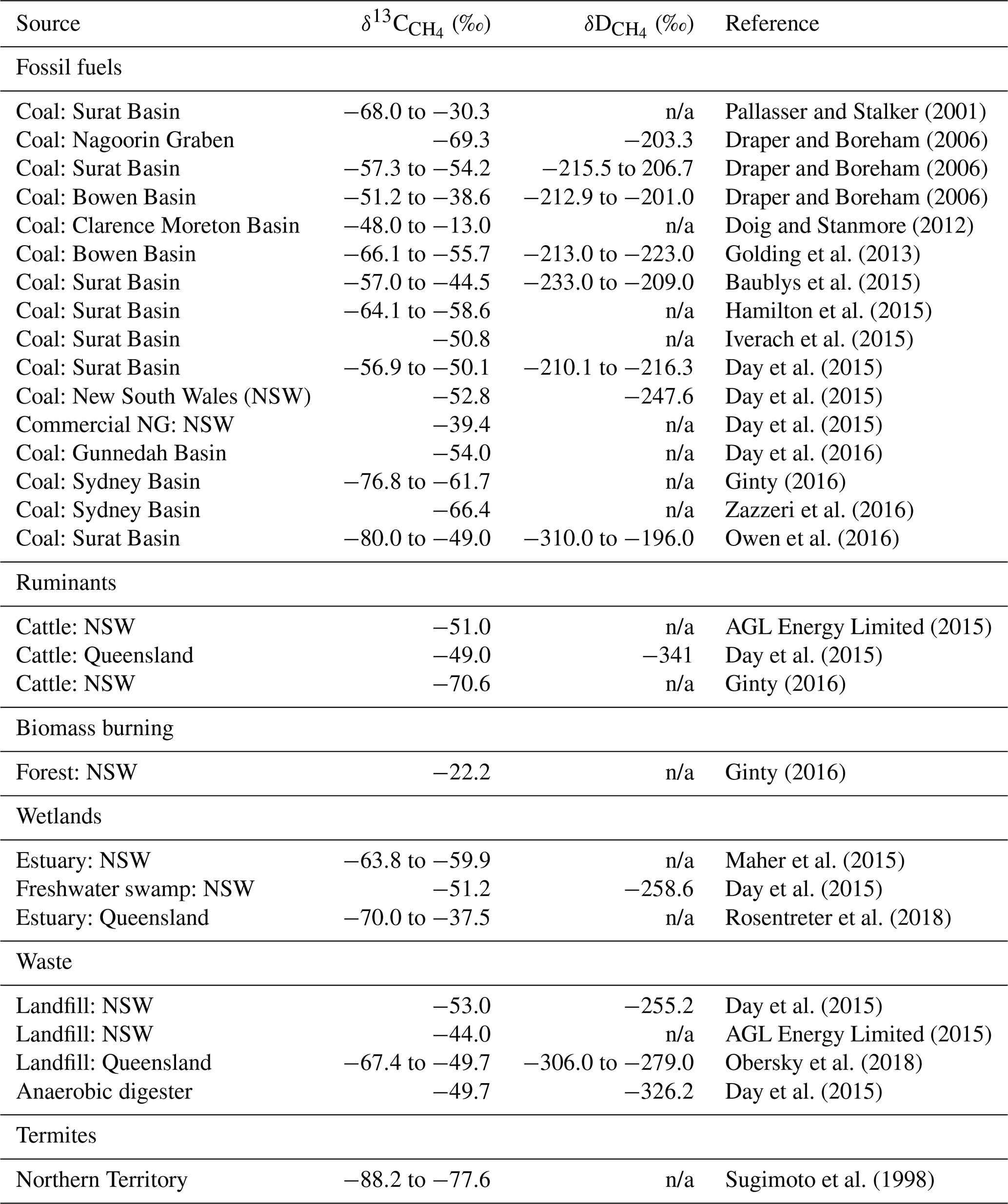
Isotope mixing models can be used for both regional- and global-scale studies to provide strong constraints on sources and sinks (Beck et al., 2012; Fisher et al., 2017; France et al., 2016; Lowry et al., 2020; McNorton et al., 2018; Nisbet et al., 2016, 2019; Rice et al., 2016; Rigby et al., 2017; Röckmann et al., 2016; Schwietzke et al., 2014, 2016; Tarasova et al., 2006). However, there is a wide range of reported CH4 isotopic signatures (Sherwood et al., 2017). It is therefore important to establish suitable source signatures for the sources of interest at the regional scale. Sherwood et al. (2017) identified gaps in the isotopic characterization in Australia. Whereas the isotopic composition of conventional fossil fuel sources is relatively well defined, there are few studies with isotope information of unconventional fossil fuels and even fewer for other CH4 sources such as ruminants and waste. Table 1 lists literature-reported isotopic signatures for typical CH4 sources in Australia in addition to those listed in Sherwood et al. (2017), which illustrates the large variability in measured signatures across and within geographies.
Here we present mobile CH4 surveys that identify and characterize major CH4 sources in the CSG fields in south-eastern Queensland. Only plumes from clearly isolated sources or individual facilities were sampled as detailed below. Measurements of and from grab bag air samples are then used to determine the source signature for the isolated source. These results improve the database on the isotopic signature of CH4 sources in Australia, and in particular the Surat Basin. We also assess the usability of measuring just or whether both and are needed to differentiate between sources.
2.1 Study area
The study area is situated in the Condamine region, south-eastern Surat Basin, and spans from Toowoomba, Dalby, and Chinchilla to Miles and the surrounding area. The size of the total study area is approximately 50 000 km2. Figure 1 shows potential major sources of CH4 in the study area. Location and capacity data (where available) of CSG wells, petroleum pipelines, coal mines, cattle feedlots, piggeries, landfills, wastewater treatment plants (WWTPs), and abattoirs (export abattoirs that include both meat works and additional processing and smaller licensed abattoirs) were retrieved from the Queensland Government Open Data Portal (https://www.data.qld.gov.au, last access: 16 June 2020). CSG processing facilities and raw water ponds were manually located using Google Maps (Google LLC, USA) and Queensland Globe (Queensland Government, 2020a). The locations of ground seeps discussed are a combination of those reported in Day et al. (2015) and field measurements. In Day et al. (2015) and this study, ground seeps refer not only to natural CH4 seeps, but also to abandoned exploration wells.
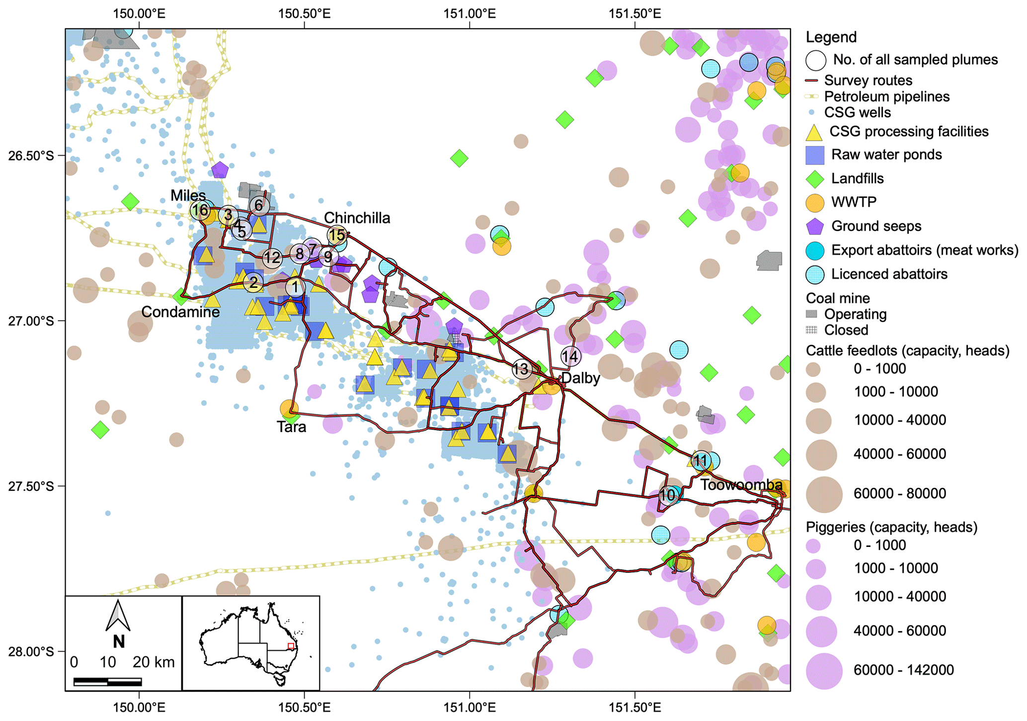
Figure 1Map of the study area with survey routes and potential CH4 sources. Inset map shows the location in south-eastern Queensland (inset map data: Australian Government, 2020, Administrative Boundaries © Geoscape Australia). The positions of the sampled CH4 plumes are numbered 1 through 16.
The Surat Basin holds more than 60 % of Australia's total proven gas reserves (Australian Competition and Consumer Commission, 2020). The study area covers many of the intensive CSG exploration and production petroleum leases (PLs). In 2018 gas was produced from 5153 exploration, appraisal, and production CSG wells as well as a small number of oil and coal exploration wells within the region (Queensland Government, 2020b). All the CSG in the Surat Basin is produced from the Walloon Coal Measures (WCM; Queensland Government, 2020c). Within the region there are 42 processing facilities, 21 raw water ponds, and over 2000 km of pipelines. To the east and north of the CSG region studied there are four operating open-cut coal mines and one that recently closed. In total, they produced 17.5 million tonnes of saleable coal from 1 July 2018 to 30 June 2019 (Queensland Government, 2019). Coal- and gas-fired power stations are another potential source of CH4. In the study area, seven power stations (five CSG-fired and two coal-fired) are operational; together they account for 0.15 % of the CH4 emissions for the south-eastern portion of the Surat Basin CSG fields (Neininger et al., 2021). CH4 sources from the agricultural sector are also considerable. Cattle and pigs are two of the most important commodities in Queensland. There are also other anthropogenic sources of CH4 in the town areas, including landfills, WWTPs, domestic wood heaters, and automobiles. Natural CH4 seeps (the Condamine River near Chinchilla) and emissions from abandoned coal exploration wells have also been mapped within the region (Day et al., 2013, 2015; Iverach et al., 2014; Kelly et al., 2015, 2017; Kelly and Iverach, 2016).
Ruminants such as cattle produce CH4 in the rumen, which is then emitted into the atmosphere. A study from the Australian Commonwealth Scientific and Industrial Research Organisation (CSIRO) reported that cattle grazing is the main contributor to the total regional CH4 emissions in the Surat Basin. Two sources of community concern, CSG and feedlots, contribute less to the regional emissions than the grazing cattle (Luhar et al., 2020).
Within the Condamine Natural Resource Management Region there are ≈560 000 cattle (meat (feedlot and pasture) ≈520 000 and dairy ≈40 000) (Australian Bureau of Statistics, 2020). In 2018 there were 65 feedlots in the region, the largest, Grassdale Feedlot, holding up to 75 000 cattle (Beef Central, 2020; Queensland Government, 2018a). As part of this study, we sampled the plume downwind of Stanbroke Feedlot (no. 12 in Fig. 1) in 2018. This feedlot has a capacity of 40 000 cattle. Most cattle in the region are in the surrounding dryland farming districts. These cattle graze a variety of crops and native grasses (we label these grazing cattle). We sampled a plume from roadside-feeding grazing cattle near Dalby in 2019 (no. 13 in Fig. 1).
Pigs produce CH4 via the anaerobic degradation of organic matter by bacteria in their digestive systems. Manure in the piggeries is another source of CH4 due to processing by microbial consortia (Flesch et al., 2013). The increasing acidogenic bacteria in the manure convert substrates into volatile fatty acids (VFAs), CO2, and hydrogen [H]. The methanogenic bacteria then produce CH4 from organic acids (Monteny et al., 2006). There are 67 piggeries spread throughout the Natural Resource Management Region, collectively holding ≈270 000 pigs in 2018/19 (Australian Bureau of Statistics, 2020). In the region, the largest piggery holds up to 142 000 pigs (Queensland Government, 2018b). In 2019 we sampled a plume downwind of Albar Piggery (no. 14 in Fig. 1), which has a registered capacity of 4980 pigs.
Other agriculture-related CH4 emissions in the region are from urban waste biosolid and animal manure that are used to fertilize the soils in the irrigation districts and abattoirs. In Queensland there are many abattoirs that process meat for both domestic use and export. The number of abattoirs documented in the area is 20; most of these abattoirs are small (licensed abattoirs), but there are two large export abattoirs: Beef City (Abattoir A; no. 10 in Fig. 1) and Oakey Beef Exports (Abattoir B; no. 11 in Fig. 1). Beef City is one of only two comprehensive beef-processing plant and feedlot operations in Australia and is one of the largest such facilities worldwide. The feedlot has a capacity of 26 500 head, and 1134 cattle are processed in the beef-processing plant per day. Oakey Beef Exports processes up to 1200 head of cattle per day (NH Foods, 2020). Both facilities produce a range of meat and meat by-products.
Urban landfills are strong sources of atmospheric CH4 (Nisbet et al., 2020). Isotopic signatures of gas emitted from landfill gas collection systems or covering soil vary depending on factors such as deposited materials, temperature, or the degree of CH4 oxidation in the above-soil layers (Zazzeri et al., 2015). As part of this study, we sampled the plume downwind of the Chinchilla domestic landfill (26.74∘ S, 150.60∘ E; no. 15 in Fig. 1). The landfill has a disposal area of approximately 0.07 km2 for municipal waste and was closed to the public in 2014. This landfill is typical of many small-town landfills in the region, and when operational it accepted mixed dry and solid organic domestic waste and commercial and industrial waste. These landfills have a simple design and typically have a clay lining and soil cover. A full listing of the landfills in the study area and the materials deposited within each are listed in Western Downs Regional Council (2021a).
WWTPs are another source of urban CH4 emissions, and there is a treatment plant at every major town in the region. In 2019 we sampled the plume immediately downwind of the Miles WWTP (no. 16 in Fig. 1). There, the sludge was treated in digestion tanks under anaerobic conditions. The liquid from the tanks was then transferred to the aerobic lagoons for further purifying (Western Downs Regional Council, 2021b).
Natural sources in the region include wetlands, termites, and natural fires by lightning (Lu et al., 2020). We did not attempt to characterize these natural sources as part of this study. Below we focus on the major anthropogenic sources identified in Luhar et al. (2018, 2020).
2.2 Mobile CH4 monitoring system
To map the major CH4 sources in the Surat Basin, we measured the CH4 mole fraction in the atmosphere as we drove along the main roads throughout the major CSG and agricultural regions of the Surat Basin. In 2018 and 2019 over 2000 km of measurements were made using a Los Gatos Research Ultraportable Greenhouse Gas Analyser (LGR-UGGA) (model 915-0011, Los Gatos Research, Inc., USA). This instrument uses off-axis integrated cavity output spectroscopy (Baer et al., 2002) and records the CH4 mole fraction every second in parts per million (ppm). The manufacturer's stated precision is 1 standard deviation of <2 ppb and a measurement range of 0 to 100 ppm. These analysers were further characterized by Allen et al. (2019). Infield calibration using Southern Ocean air supplied by CSIRO is discussed further below. The air inlet was attached to a mast mounted on top of the vehicle (2.7 m above the ground surface). Ambient air was then pumped into the LGR-UGGA through a Teflon tube. A Hemisphere global positioning system (GPS) (model A326, Hemisphere GNSS, Inc., USA) was also mounted on the roof, measuring the geolocation to within 8 cm (2 standard deviations; Hemisphere GNSS, 2015). The air inlet tube was 2.5 m long; this results in a lag between the GPS-recorded time stamp and the analyser time stamp. Using standard air this was determined to be 7 s. It was not the goal of the project to do detailed plume analyses. Driving speed was not independently continuously measured, and only a lag time correction was made. As a result, the surveys were not precisely positioned. When a major plume was traversed, we returned to the centre line of the plume and remained stationary to georeference the plumes shown in Fig. 2. The car was stationary for up to half an hour while the air samples were collected. In Fig. 2 the plume positions are accurately located, but away from the plumes the survey results are only approximate to within the order of tens of metres.
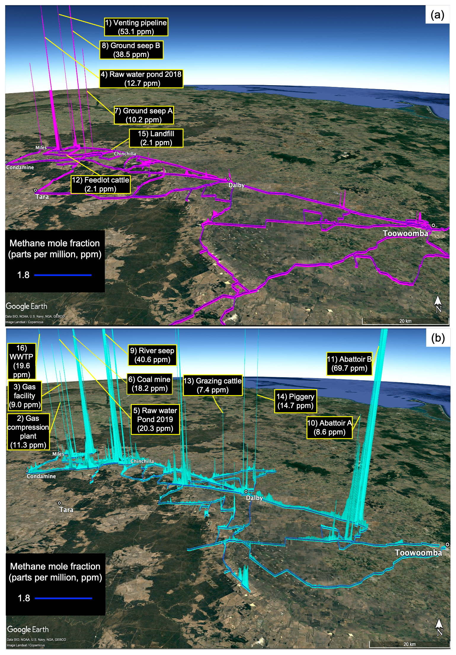
Figure 2The vehicle-mounted CH4 survey routes throughout the Surat Basin. Daytime measurements are represented by a magenta ribbon and nighttime measurements by a cyan ribbon. A linear scale is used to represent the measured CH4 mole fraction. For all sampled plumes, the highest recorded CH4 mole fraction is indicated (image ©Google Earth).
For a small portion of the 2018 campaign, plume mapping was done using a Picarro G2201-i cavity ring-down spectrometer (CRDS) (Picarro, Inc., USA), due to the failure of the LGR-UGGA unit. The Picarro-reported precision (1 standard deviation, 30 s average) of CRDS for a CH4 mole fraction is 5 ppb+(0.05 % of the reading) for 12C and 1 ppb+(0.05 % of the reading) for 13C in high-precision (HP) mode with an operational range of 1.2 to 15 ppm. Under the same operation mode, the instrument precision (1 standard deviation, 5 min average) for is <1.15 ‰ with a maximum drift (over 24 h) of <1.15 ‰ at 10 ppm. Previous studies have also characterized the Picarro G2201-i performance (e.g. Assan et al., 2017; Rella et al., 2015). For the Picarro portion of the surveying we recorded the GPS location using a Kinetic Lite GPS application (Mothership Software Ltd., UK). Using the standard air, we determined the time lag between the real-time GPS location reading and the display of mole fraction reading on the Picarro G2201-i CRDS to be 3 min and 40 s. Using this timing offset, we adjusted the time stamp for the analyser data.
One-point calibrations for the two instruments were conducted before and after each survey using Southern Ocean air provided by CSIRO. The calibration gas was placed into 3 L SKC FlexFoil PLUS sample bags (SKC Inc., USA) for shipping and analysed at the greenhouse gas laboratory of Royal Holloway, University of London (RHUL), to determine the for the calibration air ( ‰). RHUL also measured the CH4 mole fraction of the calibration gas (1801.2±0.5 ppb). The isotope value measured by RHUL ( ‰) also closely resembles the value from flasks ( ‰, mean±standard deviation for 12 flasks collected) collected at Cape Grim and measured at the Institute of Arctic and Alpine Research (INSTAAR), University of Colorado (White et al., 2018), around the same time as the Southern Ocean cylinder was filled by CSIRO (29 June 2016 to 11 August 2016). The infield standard deviations for mean CH4 mole fraction measurements of the reference standard across all days were 4.9 (2018) and 9.6 ppb (2019) for LGR-UGGA and 5.3 ppb (2018) for Picarro G2201-i CRDS. This repeatability is better than reported in Takriti et al. (2021).
2.3 Sampling and measurement methods
During the two campaigns in 2018 and 2019, driving speed was controlled between 10–80 km h−1 for surveys with LGR-UGGA and 10–40 km h−1 for surveys with Picarro G2201-i CRDS where traffic conditions were suitable. The lower driving speed coupled with real-time CH4 mole fraction readings allowed us to detect plumes associated with potential CH4 sources. When a constant plume was detected, we collected 10 air samples for isotopic analysis downwind of the plume by pumping air into 3 L SKC FlexFoil PLUS sample bags with polypropylene fittings using a 2 L medical syringe. In total, over 160 air samples were collected from 16 major sources in the Surat Basin CSG fields. On the day the samples were collected they were analysed for CH4 mole fraction and in the field using Picarro G2201-i CRDS for data quality-control purposes. In 2018 the root-mean-square error (RMSE) between the University of New South Wales (UNSW Sydney) Picarro 2201-i CRDS and the RHUL Picarro G1301 CRDS (detailed below) was 0.437 (ppm; Fig. A1a) and in 2019 the RMSE between the UNSW Sydney Picarro 2201-i CRDS and the Institute for Marine and Atmospheric research Utrecht (IMAU) continuous-flow isotope ratio mass spectrometry (CF-IRMS) (detailed below) was 0.232 (ppm; Fig. A1b).
The sampling of plumes favours those sources that happen to be upwind and close to a public road. The objective of this study was not to quantify the emission rate (flux) of individual sources. Rather, our aim was to characterize the isotopic source signatures of potential significant sources of CH4 in the region. We did not have permission to access private properties or industrial sites, which was a significant constraint on sampling. All samples collected in this study are from publicly accessible locations. When a plume was located, we sampled several locations within the plume to maximize the range of CH4 mole fraction values that could be obtained within the limits of public access. Sampling a large range of CH4 mole fraction values assists with minimizing the uncertainties for each source signature derived using the Keeling plot method in combination with Bayesian linear regression (see Sect. 2.4).
In 2018, air samples were analysed in the greenhouse gas laboratory at RHUL for CH4 mole fraction and using the Picarro G1301 CRDS (Picarro, Inc., USA) and modified gas chromatography isotope ratio mass spectrometry (GC-IRMS) system (Trace Gas and Isoprime mass spectrometer, Elementar UK Ltd., UK) respectively. The Picarro G1301 CRDS was calibrated to the WMO X2004A scale using NOAA (National Oceanic and Atmospheric Administration) air standards (Dlugokencky et al., 2005; Fisher et al., 2006, 2011; WMO, 2020). For CH4 mole fraction analysis, each sample was analysed for 210 s on the Picarro G1301 CRDS with a reproducibility of ±0.3 ppb, and the mean CH4 mole fraction of the last 90 s of the analysis was recorded. For analysis, samples with mole fractions above 6 ppm were diluted with zero-grade nitrogen to fit the dynamic range for the GC-IRMS and then measured in triplicate on the VPDB (Vienna Pee Dee Belemnite) scale. A fourth analysis was made if the standard deviation of the first three analyses was greater than the target instrument precision of 0.05 ‰. A portion of the samples (from 13 plumes) was further analysed in the IMAU for CH4 mole fraction, , and using continuous-flow isotope ratio mass spectrometry (CF-IRMS) (Thermo Finnigan Delta plus XL, ThermoFinnigan MAT, Germany) (Brass and Röckmann, 2010; Eyer et al., 2016). All samples were measured directly with the automated extraction system. For the subsequent IRMS measurements, the CH4 in the air from most bags was preconcentrated for 10 min at a flow rate of 6 mL min−1 for and 4 mL min−1 for , but for samples reported by RHUL that had a CH4 mole fraction larger than 6 ppm, the samples were processed for a shorter time in order to extract a quantity of CH4 similar to the reference air. The CH4 from 60 mL of air was extracted for each measurement and from 40 mL for measurements. measurements are given on the VSMOW (Vienna Standard Mean Ocean Water) scale. A one-point calibration was done using a reference cylinder with the following assigned-value CH4 mole fractions: 1975.5 ppb, : −48.2 ‰ (VPDB), : −90.8 ‰ (VSMOW). In 2019, air samples were analysed at IMAU for CH4 mole fraction, , and using the same CF-IRMS as 2018. Samples with a reported CH4 mole fraction larger than 3 ppm by UNSW Sydney were sampled at a lower flow rate in order to extract a quantity of CH4 similar to the reference air. A one-point calibration was done using a reference cylinder with the following assigned-value CH4 mole fractions: 1970.0 ppb, : −48.1 ‰ (VPDB), and : −88.3 ‰ (VSMOW). Due to the high precision of the RHUL GC-IRMS measurements of <0.05 ‰ for δ13C and the IMAU IRMS measurements of <0.1 ‰ for δ13C and <2 ‰ for δD, reliable source signatures can usually be derived for elevations of 100–200 ppb above the background.
2.4 Data analysis
The and for CH4 sources of each detected plume were determined using the Keeling plot approach (Keeling, 1958; Pataki et al., 2003) shown in Eq. (1):
where [CH4(b)] and δ(b) are the CH4 mole fraction and (or ) of the background air, [CH4(a)] and δ(a) are the CH4 mole fraction and (or ) of the atmosphere, and δ(s) is the (or ) of the mean source respectively. The intercept (δ(s)) of the linear regression between δ(a) and represents the isotopic signature of the source mixed in the background ambient air. The Keeling plot method requires the background air CH4 mole fraction and isotopic signature to be constant during the period of observation. The time it takes to collect the 10 samples is approximately 30 min, and normally the background air composition does not change during the period of sampling. The mobile survey readings show that the background CH4 mole fraction was stable in 2018 and 2019 daytime and nighttime surveys (Fig. A2), which supports this assumption. For each Keeling data set the linear regression line and credible interval (analogous to the confidence interval) were determined using the PyMC3 Bayesian regression package (Salvatier et al., 2016). The regression methodology was selected based on the fact that there are bivariant correlated errors in both the x and y variables (e.g. Miller and Tans, 2003; Zazzeri et al., 2016) and that the number of samples in each plume set was small (≤10). Bayesian regression was used since it is a robust algorithm that balances uncertainty in both the x- and y-axis data (Jaynes, 1999), it is suitable for small data sets (Baldwin and Larson, 2017), and it has been demonstrated to yield more reliable isotopic signatures at low mole fractions with low sample numbers (Zobitz et al., 2007).
3.1 Regional plume mapping and the benefits of sampling at nighttime
Two campaigns with over 2000 km routes were conducted in September 2018 and from August to September 2019 (Fig. 1). The CH4 mole fraction in the atmosphere 2.7 m above the ground was mapped between Toowoomba and Miles (a distance of approximately 200 km). Surveys of CH4 mole fraction during both daytime and nighttime are shown in Google Earth (Fig. 2). In 2018, we did not detect plumes from coal mines, river seeps, abattoirs, piggeries, or WWTPs, and thus we shifted our focus from daytime surveying in 2018 to nighttime surveying in 2019. During the day the sunshine heats the ground, which warms the air immediately above the surface. This causes the plumes to rise rapidly and mix with background air within the growing boundary layer rather than accumulating within the nocturnal boundary layer. This results in daytime plumes either being missed during the mobile surveys or having a limited range of CH4 mole fraction values. By contrast, at night during light to moderate wind conditions, the plumes typically disperse slowly within the stable nocturnal boundary layer when there is a large temperature inversion (Stieger et al., 2015). This enabled us to sample isolated source plumes that have a greater spread of CH4 mole fraction, which improves determination of the line of best fit in Keeling plots and minimizes the uncertainties of the derived isotopic source signatures. As part of developing an inventory (Neininger et al., 2021) in the region, all major CH4 sources were located and were georeferenced to guide nighttime sampling. Also, most facilities were well lit, which assisted with source identification. The contrast in the magnitude of the CH4 mole fraction measured in the field between the daytime and nighttime surveys is clearly visible in Fig. 2. The distribution of the CH4 spikes demonstrates the complex spread of the sources in the study area. Overall, measured CH4 mole fraction ranged from 1.8 to 69.7 ppm – the highest value was recorded in a plume downwind of Oakey Beef Exports (Abattoir B).
3.2 Source isotopic signatures
The Keeling plot results of CH4 source signature calculations are listed in Table 2 and shown in Fig. 3, and the Keeling plots are shown in Figs. A3–A7 in Appendix A. For each (‰) and (‰) isotopic signature both the posterior standard deviation and the credible interval were determined. The variability in the credible interval is primarily due to both the sampled CH4 mole fraction range and the number of data points used in the Keeling plot analysis as shown in Fig. A8.
Table 2CH4 source signature results for plumes sampled in the Surat Basin 2018 and 2019 campaigns. CH4 excess over background (ppm) for the samples that were used to calculate the source signature are presented, and (‰) and (‰) are reported along with the Bayesian posterior distribution mean, standard deviation, and 95 % credible interval (in brackets). n/a: not applicable.
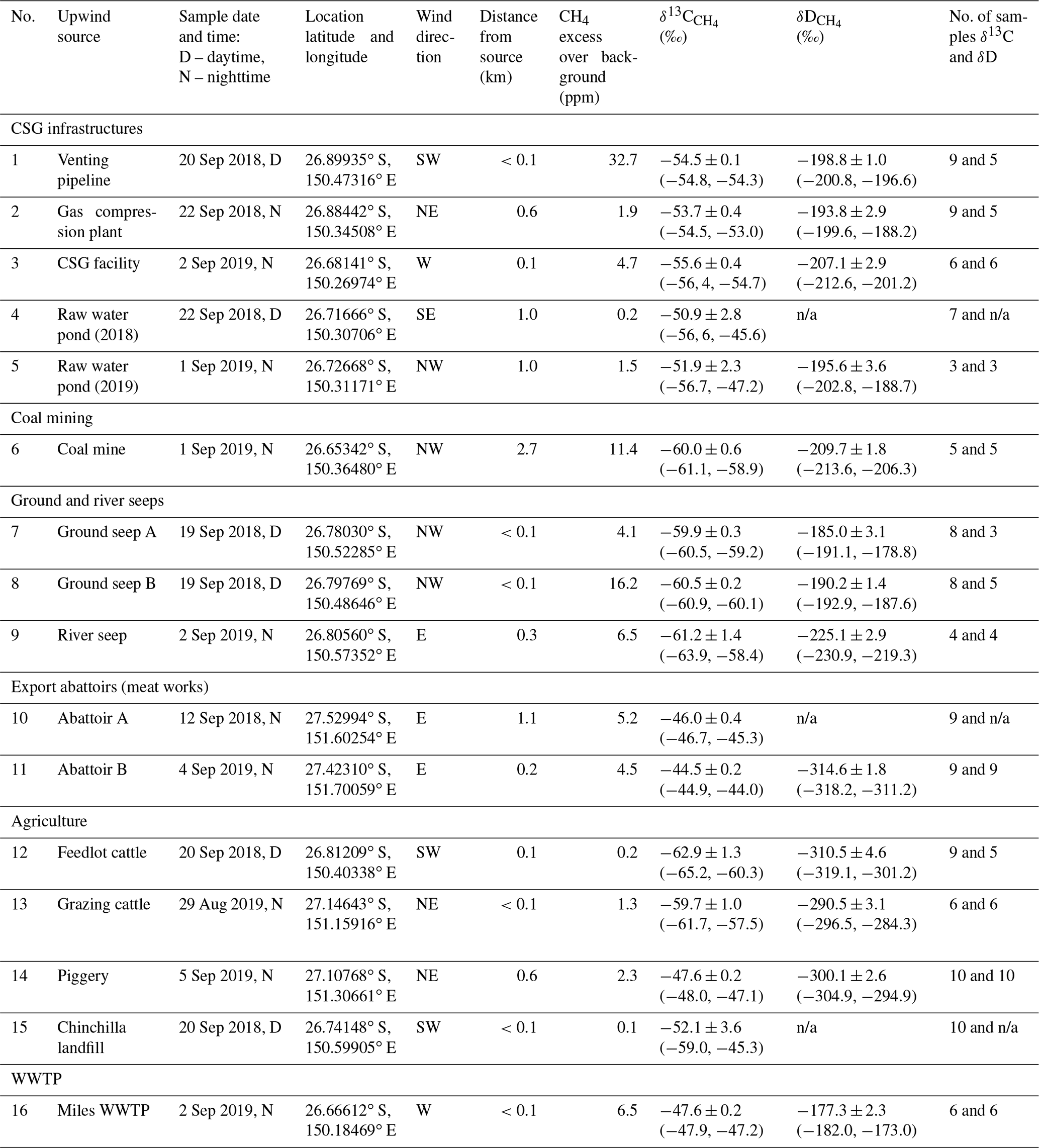
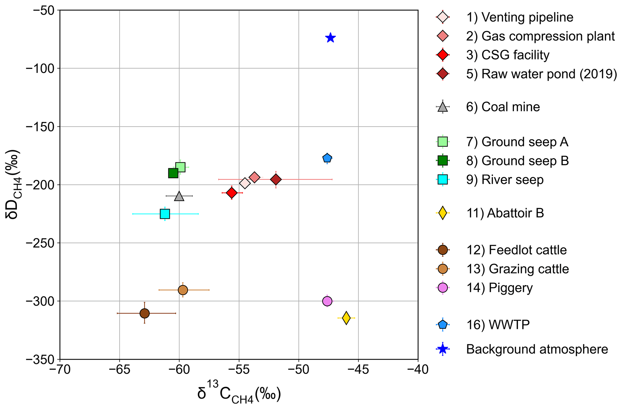
Figure 3Dual isotope plot of all measured CH4 sources in the study. For markers with missing error bars the Bayesian credible intervals were smaller than the symbol size. Please refer to Table 2 for detailed information of plotted data.
3.2.1 Coal seam gas infrastructures
There are many portions of the CSG production and processing life cycle where CH4 can be released, either accidentally or by deliberate venting. CH4 can be released intentionally at high-point vents along the produced water pipelines, outgassed from raw water ponds, or released as part of other venting or flaring operations. Unintentional CH4 releases can occur anywhere where there are joints and seals, which can be at well heads, or along gas distribution lines, compression stations, and processing plants. The isotopic signatures of the resultant CH4 emissions may vary depending on the origin of the gas within a gas field. The production processes and conditions of the coal and associated groundwater are not constant throughout a region, which can result in variations of the isotopic composition of the gas both spatially and with depth (Hamilton et al., 2015; Iverach et al., 2017). In the Surat Basin CSG fields, all CH4 plumes from active CSG production and processing sources sampled show relatively little variability and sit in a distinct cluster isolated from non-CSG sources in Fig. 3. These plumes were from a range of sources including a high-point vent on a produced water pipeline, a gas compression plant, a raw water pond (measured in both the 2018 and 2019 campaigns), and a CSG facility (nos. 1–5 in Table 2 and Figs. 1–3).
Downwind of the high-point vent on the produced water pipeline, we sampled a plume with a maximum CH4 mole fraction reading of 35.0 ppm (wind direction was SW) approximately 15 m from the venting point (no. 1 in Table 2 and Figs. 1–3). The and signatures of the vented gas were ‰ and ‰.
Another major CSG CH4 plume detected was associated with nighttime operations at the APLNG Talinga gas compression plant (no. 2 in Table 2, Figs. 1–3). On the evening of sampling, this plume extended for 17 km (see Fig. 2). The peak CH4 mole fraction measured was 11.3 ppm approximately 0.6 km downwind of the facility. The sampled gas had and signatures of ‰ and ‰ respectively.
The Glen Eden raw water pond was surveyed on 22 September 2018 and 1 September 2019 (nos. 4 and 5 in Table 2, Figs. 1–3). This pond is one of the many infield storages that temporarily hold water gathered from each CSG well head (QGC, 2014). The signatures of the gas sampled were ‰ and ‰ in 2018 and 2019 respectively, with a signature of ‰ in 2019. No significant differences were found between the signatures from the two campaigns for this pond. The results are similar to those from a previous study in the area with a signature of −50.8 ‰ (90 % CI, −55.7 ‰ to −45.8 ‰) from CSG water storage (Iverach et al., 2015).
In September 2019 we intersected a CH4 plume emanating from a CSG gas transfer hub. The peak CH4 mole fraction measured in the plume 150 m east and downwind of the facility was 7 ppm. The and signatures were 55.6±0.4 ‰ and ‰ respectively (no. 3 in Table 2, Figs. 1–3).
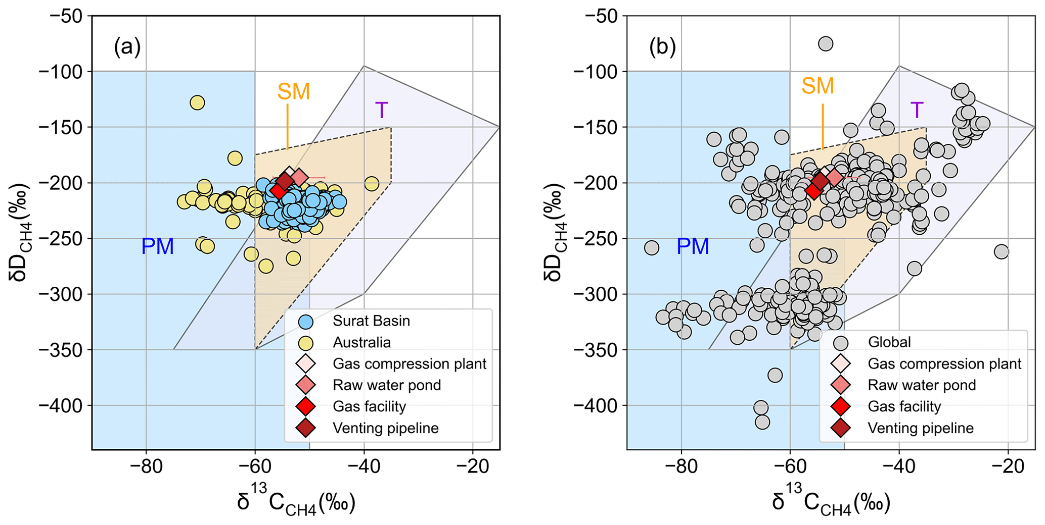
Figure 4A comparison of and of CSG from this study versus values from the Surat Basin, Australia-wide (a) and worldwide (b). All values are taken from Sherwood et al. (2017) and literature sources listed in Table 1. The gas genetic fields are taken from Milkov and Etiope (2018). PM: primary microbial; SM: secondary microbial; T: thermogenic.
Draper and Boreham (2006) reported that the signature for CH4 from the Surat Basin WCM ranged from −57.3 ‰ to −54.2 ‰, indicating secondary biogenic CH4 with a minor thermogenic component. More recent studies by Hamilton et al. (2014, 2015) and Baublys et al. (2015) report a signature ranging from −64.1 ‰ to −44.5 ‰ with a median of −52.0 ‰. These have a range of approximately 20 ‰, while all above-ground measurements fall within a narrower range. Iverach et al. (2015) and Day et al. (2015) reported signatures from −56.9 ‰ to −50.1 ‰, and in this study we measured signatures from ‰ to ‰ (Fig. 4). Owen et al. (2016) found that the values for the gas reservoir (200–500 m) for coal measures in the Surat Basin were between −58.0 ‰ and −49.0 ‰. This is consistent with our study as the commercially produced gas is extracted from coal seams at depths >200 m (Queensland Government, 2020b).
The data for the WCM in the Surat Basin are relatively sparse in the literature. Early studies of the Surat Basin CSG found a range of signatures from −215.5 ‰ to −206.7 ‰ (Draper and Boreham, 2006). Baublys et al. (2015) and Day et al. (2015) reported that gas from the WCM in the same area had values from −233.0 ‰ to −209.0 ‰ and from −216.3 ‰ to −210.1 ‰. In general, the determined signatures ( ‰) of gas from CSG infrastructures in this study are approximately 23 ‰ less depleted than previous studies ( ‰) but fall between −310 ‰ and −196 ‰ reported by Owen et al. (2016). In Fig. 4, the data from this study are compared with and values reported for CH4 sourced from coal seams in Australia (Fig. 4a) and worldwide (Fig. 4b) (Sherwood et al., 2017). The distribution of the data from this study sits within the secondary microbial area of the CH4 genetic diagram (see Fig. 4), which provides evidence that gas in the WCM has a secondary biogenic origin with a thermogenic component.
3.2.2 Coal mining
On 1 September 2019 samples were collected from a plume downwind of the Cameby Downs open-cut coal mine located approximately 16 km north-east of Miles (no. 6 in Table 2 and Figs. 1–3). This is one of the largest coal mines in Australia, with permission to extract up to 2.8 million tonnes per annum (Mtpa) of run-of-mine coal (Yancoal, 2018). The measured CH4 mole fraction was between 2 and 13 ppm north-east of the coal mine. The sampled downwind plume from the Cameby Downs open-cut coal mine yielded and signatures of ‰ and ‰ respectively (see Table 2). These values are close to the values measured as part of this study from the ground seeps (abandoned coal exploration wells) (see Fig. 3) and sit within the range of the global and Australian CSG sectors (see Fig. 4). These results are expected because the signatures from coal mines depend on coal rank and the process of secondary biogenic CH4 generation (Zazzeri et al., 2016). Coals from the Cameby Downs mine are sub-bituminous to high-volatile bituminous (Hamilton et al., 2014) extracted from the relatively shallow Juandah measure (<200 m) in the Walloon Subgroup. Our results are consistent with the values from Owen et al. (2016), which suggests the shallow coal measures have and signatures ranging from −80 ‰ to −50 ‰ and from −310 ‰ to −210 ‰ respectively.
3.2.3 Ground and river seeps
Within the Surat Basin the origin of the CH4 associated with seeps mapped at various roadside locations or along the Condamine River west of Chinchilla is poorly characterized (Day et al., 2013, 2015; Iverach et al., 2015; Nisbet et al., 2020). In our study during the 2018 and 2019 campaigns, two ground seeps and one river seep of CH4 were characterized (nos. 7–9 in Table 2, Figs. 1–3). Both ground seeps (believed to be coal exploration wells) are located along Green Swamp Road. At each site we sampled from near the plume centre (likely over the old borehole) to approximately 50 m away downwind to obtain a spread of CH4 mole fraction and isotopic composition data for Keeling plot analysis. The peak CH4 mole fractions measured in the bag samples from seep A and seep B were 6 and 18 ppm. Seep A had and signatures of ‰ and ‰. Seep B had and signatures of ‰ and ‰. The two ground seeps were also investigated in previous studies made by UNSW Sydney and RHUL, which reported of −56.9 ‰ for gas collected from seep B (Day et al., 2015) and of −60 ‰ (Iverach et al., 2014). The isotopic signatures indicate that the gas could originate from coal seams. We were able to visually confirm pieces of historical coal exploration, and it was stated in Day et al. (2015) that exploration drilling occurred at seep B during the 1970s. This is supported by the data available from the Queensland Government, which show a plugged and abandoned borehole at the same location. These likely coal seam sourced ground seeps have and signatures that align with the more depleted biogenic values (less than 55 ‰) of global coal gas and have slightly enriched compared to Australian coal gas (see Fig. 4).
Many CH4 seeps have been located in the Condamine River, suggesting that the emitted CH4 is associated with coal seams in the area (Day et al., 2013; Department of Natural Resources and Mines, 2012). On 2 September 2019, we intersected CH4 plumes near the Chinchilla weir and measured CH4 mole fractions as high as 18 ppm in calm to light wind conditions (0–14 km h−1). Gas samples had and signatures of ‰ and ‰ respectively. These values are similar to the results from the coal mine sampled in the study area (see Fig. 3). The value is also consistent with the results previously reported from gas samples collected in the Condamine River, with values ranging from −63.4 ‰ to −59.3 ‰ (Department of Natural Resources and Mines, 2012). Iverach et al. (2017) proposed a hydrogeological conceptual model and CH4 production evolution model between the WCM and the overlying Condamine River alluvial aquifer, indicating the upward migration of CH4 from the WCM. The relatively depleted signature we measured is comparable to the values (−69.1 ‰) of CH4 believed to originate from shallow WCM in Iverach et al. (2017). The and signatures also align with the values from Owen et al. (2016), showing that CH4 from shallow coal measures (<200 m) have and signatures ranging from −80 ‰ to −50 ‰ and from −310 ‰ to −210 ‰ respectively.
3.2.4 Abattoirs
High CH4 mole fractions have been observed from intensive meat-processing facilities in the study area (Nisbet et al., 2020). We sampled the plumes downwind of Beef City abattoir (Abattoir A) in 2018 and Oakey Beef Exports (Abattoir B) in 2019 (nos. 10 and 11 in Table 2 and Figs. 1–3).
The highest CH4 mole fraction measured for Beef City was 8.6 ppm, recorded on Toowoomba Cecil Plains Road 1.3 km downwind of the complex. The Beef City plume samples yielded a signature of ‰. Beef City is an integrated feedlot and processing plant.
As part of the 2019 campaign, we sampled a CH4 plume 1 km downwind of Oakey Beef Exports (Abattoir B). This plume extended north-west of the facility. The highest CH4 mole fraction measured was 69.7 ppm, and the signature was determined to be ‰. Emissions from Oakey Beef Exports have four potential sources, including (a) the cattle themselves, (b) emissions from anaerobic lagoons, (c) emissions from biogas storage and combustion (from the facility exhaust stack), and (d) by-products and animal wastes (paunch and manure). During the sampling night, smoke was observed continuously emitting from the stack associated with the main processing plant. We sampled in the centre line of that plume, but the other three potential sources must be considered, and it is likely that we sampled a mixed source plume. The processing plant is equipped with a waste-to-energy system that integrates biowaste treatment with biogas storage, processing, and combustion. In the system, the biowaste is put in covered lagoons where anaerobic digestion occurs. In the anaerobic lagoons, concentrated anaerobic bacteria digest organic matter from Oakey Beef Export's biowaste to produce CH4. During this biogas-producing process, factors such as type of substrate, bacteria being used, and temperature can affect the isotopic signatures of produced gas. The generated biogas is stored in an on-site biogas storage tank and used to fuel the facility's boilers. The signature of ‰ from this study is more enriched compared to the values from biogas plants in Heidelberg, Germany, which are fed by maize silage ( ‰) and food waste ( ‰) (Hoheisel et al., 2019) but are close to maize-fed biogas plants in the UK (−45 ‰) (Bakkaloglu et al., 2020).
Values of from both abattoirs are similar to values from global and Australian fossil fuels (Sherwood et al., 2017). In particular, the relatively enriched compared to biogenic values suggests CH4 could be derived from the incomplete combustion of biogas, which is similar to what has been reported ( ‰) from measurement of a biogas power station in London, UK (Zazzeri, 2016). However, the signature of ‰ from Oakey Beef Exports indicates a biological origin. These results are comparable with that of a piggery sampled in our study (see Fig. 3), the anaerobic digester values (−326.2 ‰) reported in NSW, Australia (Day et al., 2015), and closely resemble the values from a biogas generator ( ‰, ‰) in Germany (Levin et al., 1993). On-site sampling at Oakey Beef Exports would be required to identify the exact source of the detected CH4 plume. These abattoir readings highlight the problem of using just to attribute the source. Using both and provides a more powerful discrimination between facility emissions from abattoirs and emissions from other gas sources.
3.2.5 Feedlot and grazing cattle
In the study area, we investigated the and signatures of CH4 emitted from Stanbroke Feedlot (no. 12 in Table 2 and Figs. 1 and 2) in 2018. The and signatures determined from the Keeling plot had values of ‰ and ‰. The peak CH4 mole fraction recorded was 3.2 ppm. In 2019 we sampled the CH4 plume emitted from over 200 cattle grazing along the roadside between Dalby and Ranges Bridge (no. 13 in Table 2 and Fig. 3). The cattle were spread from immediately adjacent to the roadside to over 100 m away. The maximum CH4 mole fraction value recorded for the grazing cattle plume was 7.4 ppm, and the and isotopic signatures were ‰ and ‰ respectively.
The isotopic signature of the cattle-produced CH4 varies depending on the diet (Levin et al., 1993). In Queensland the typical cattle diet is predominantly C4 plant with forage, grain, and supplements (McGinn et al., 2008). Specifically, due to differences in diet, the and signatures of cattle in the Surat Basin are in between the values from Levin et al. (1993) ( ‰, ‰, 60 %–80 % C4 diet) and Bilek et al. (2001) ( ‰, ‰, 90 % C3 diet) (see Fig. 5). Compared to studies in the USA, signatures in our study are more depleted than those from cattle in Townsend-Small et al. (2015) ( ‰, ‰, unspecified diet) and Townsend-Small et al. (2016) ( ‰, ‰, unspecified diet) (see Fig. 5). Both the feedlot and grazing cattle signatures determined as part of this study are generally consistent with values for ruminants around the globe and in other areas of Australia (see Table 1).
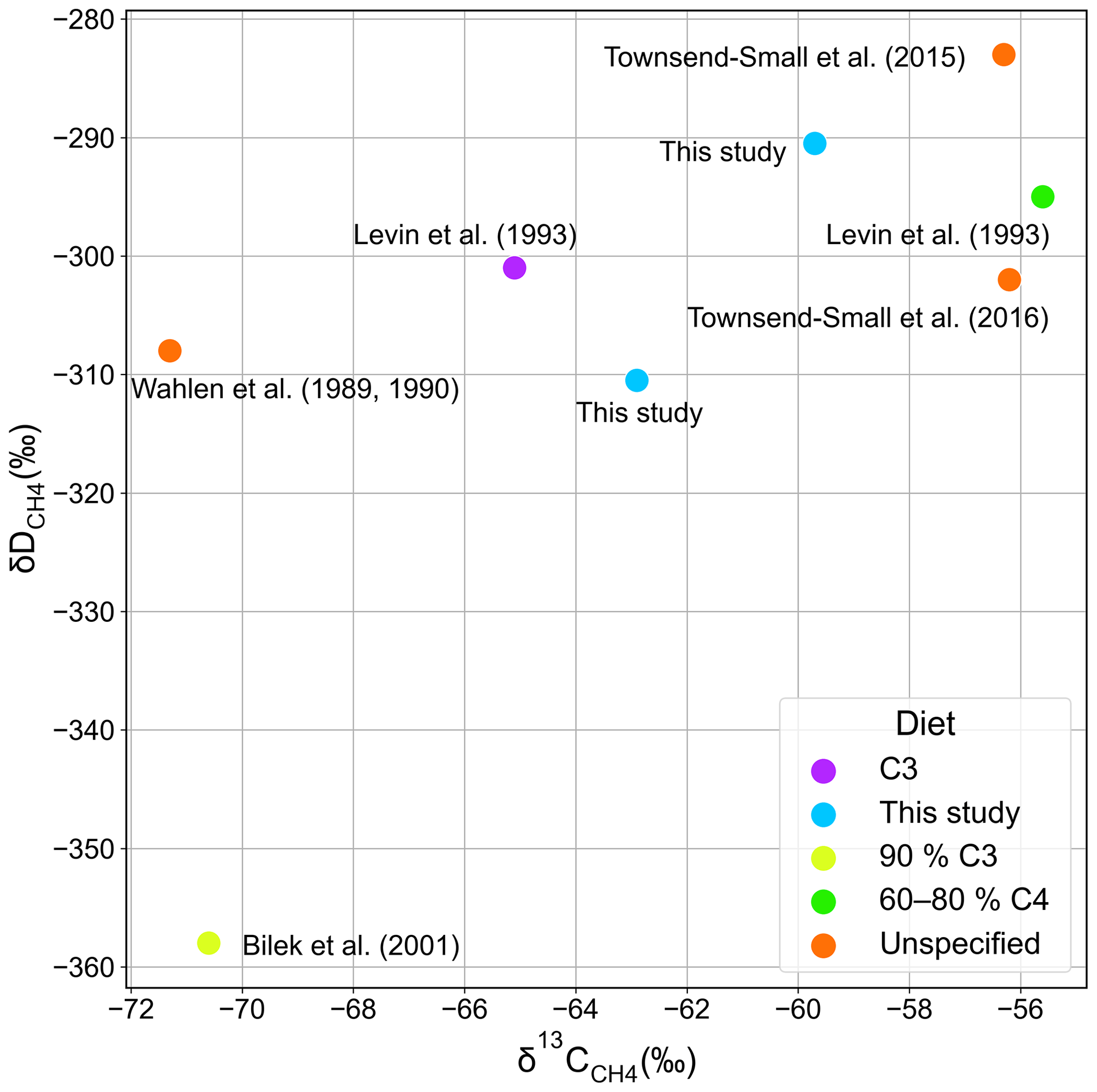
Figure 5A dual isotope plot comparing the and for cattle from this study with the values reported in the literature (indicated next to the data points).
3.2.6 Piggery
A CH4 plume was sampled 600 m downwind of Albar Piggery in 2019. This plume had a distinctive smell and a warmer temperature compared to the surrounding ambient air, indicating that the piggery was heated. The maximum CH4 mole fraction measured was 14.7 ppm, and the and signatures were ‰ and ‰ respectively (no. 14 in Table 2, Figs. 1–3). These and signatures are close to those reported by Levin et al. (1993) in Germany for lower-pile manure ( ‰ and ‰). The and values also closely resemble our results from the abattoirs (Fig. 3).
3.2.7 Landfill
Gas samples collected downwind of the Chinchilla landfill had a CH4 mole fraction range from 1.8 to 2.1 ppm and a Keeling plot best fit value of ‰ (no. 15 in Table 2 and Figs. 1–3). In general, the determined value in this study falls into the range of international and Australian CH4 sourced from waste (Table 1, Sherwood et al., 2017). The isotope ratio of CH4 in this landfill is less depleted than the mean values reported (−56.5 ‰ for surface and −58.7 ‰ for waste) of the active landfill in Ipswich, Queensland (Obersky et al., 2018), and those reported from Europe (Hoheisel et al., 2019; Xueref–Remy et al., 2020; Zazzeri et al., 2015) possibly due to CH4 oxidation by aerobic bacteria in cover soils. Similarly, relatively enriched values were also identified from older, closed landfills in the UK (Bakkaloglu et al., 2020; Lowry et al., 2020). Our result also closely resembles the value measured by Day et al. (2015), who reported −53.0 ‰ for a landfill in New South Wales, Australia, and results from the upper layers of waste (−52.0 ‰) in Germany (Levin et al., 1993).
3.2.8 WWTP
On 2 September 2019 we sampled a plume immediately adjacent to the Miles WWTP along Waterworks Road. This plume had a maximum CH4 mole fraction reading of 19.6 ppm and and signatures of ‰ and ‰ (no. 16 in Table 2 and Figs. 1–3) respectively. In Australia the of CH4 emissions from the waste sector ranges from −58.8 ‰ to −44.0 ‰ with a median of −50.4 ‰ (AGL Energy Limited, 2015; Day et al., 2015; Obersky et al., 2018; Sherwood et al., 2017); the ‰ determined for the Miles WWTP is consistent with past results. However, the signature is less depleted than the WWTP values of ‰ measured in Heidelberg, Germany (Hoheisel et al., 2019), −52.3 ‰ in Cincinnati, USA (Fries et al., 2018), and −59.2 ‰ to −50.7 ‰ in London, UK (Zazzeri, 2016), for anaerobic treatment systems. The result is similar to the measurements made by Townsend-Small et al. (2012) from two WWTPs (−46.3 ‰ and −47 ‰) in the metropolitan area of Los Angeles, USA, and result from an aerobic digestion tank of WWTPs (−45.5 ‰) in Tokyo, Japan (Toyoda et al., 2011). Both Townsend-Small et al. (2012) and Fries et al. (2018) found a more depleted for WWTPs in Los Angeles (−298 ‰) and Cincinnati (−325 ‰) compared to our result. Toyoda et al. (2011) suggested that the relatively enriched signature could be due to aerobic digestion. A better understanding of the CH4 from WWTPs in Australia is needed, especially for different treatment processes (anaerobic or aerobic), as they are proven to be non-negligible sources of CH4 emission in urban areas.
3.3 Discriminating between isotopic signatures from various sources: uniqueness and overlaps
Various studies have pointed out that there are large overlaps in CH4 isotopic signatures, compromising the use of isotopic constraints in models estimating CH4 emissions (Feinberg et al., 2018; Milkov and Etiope, 2018; Sherwood et al., 2016, 2017). Figure 6 displays probability distributions of and for fossil fuel and modern microbial processes (with their respective subcategories) in Australia (Table 1 and Sherwood et al., 2017) and around the globe (Sherwood et al., 2017). Global coal gas has a bimodal distribution and a relatively wide range spanning from −85.5 ‰ to −16.8 ‰. In Australia, coal gas has a unimodal distribution of ranging from −76.8 ‰ to −30.3 ‰ with a more depleted median of −54.3 ‰ due to the high proportion of microbial gases. Almost half of the widely spread values of coal gas have a range that overlaps with the distributions of other microbial processes. Specifically, global of cattle varies from −71.3 ‰ to −50.3 ‰ with a median of −66.5 ‰; values for Australia range from −70.6 ‰ to −49.0 ‰ with a median of −61.5 ‰. The more enriched isotopic values found in Australian cattle are likely due to higher proportions of a C4 diet (Levin et al., 1993; McGinn et al., 2008) in these tropical herds, raised on C4 grasslands and with maize supplements.
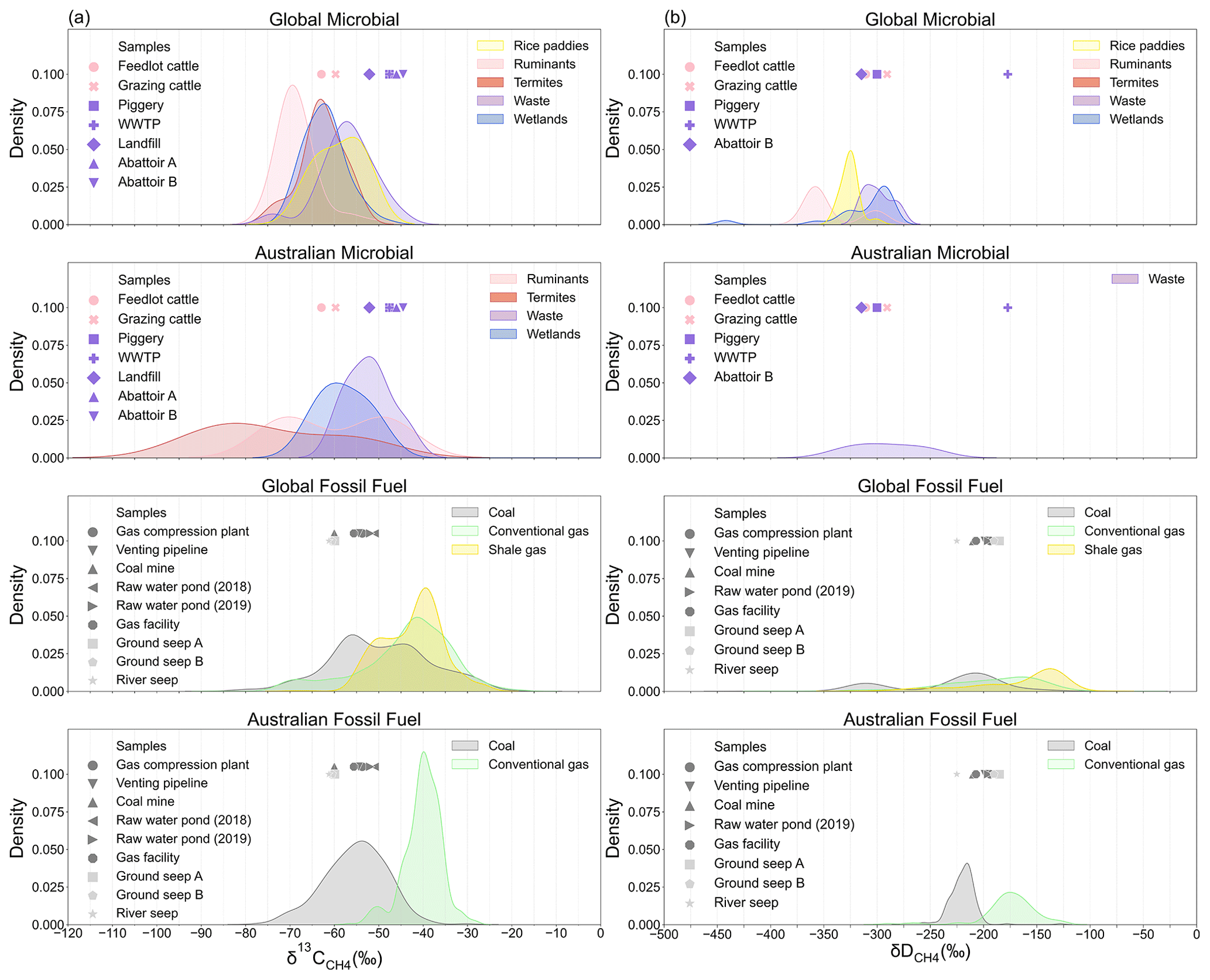
Figure 6Probability density plot of literature values (globally and from Australia) for (a) and (b) and results from this study (global values taken from Sherwood et al., 2017, and literature sources listed in Table 1).
In this study, signatures determined from CSG processing and production infrastructures and seeps varied from −61.2 ‰ to −50.9 ‰ with a median of −55.6 ‰. This range is far narrower than the global distribution of from coal presented in Sherwood et al. (2017) (Fig. 6) or those determined from gas and water well measurements (Baublys et al., 2015; Hamilton et al., 2014, 2015). The median of the CSG signature is about 6 ‰ more enriched than the signature of the cattle (which ranges from −62.9 ‰ to −59.7 ‰) and about 6 ‰ more depleted than that of waste (which ranges from −52.1 ‰ to −47.6 ‰). These similar or overlapping values for different sources mean that in areas with multiple sources like the Surat Basin CSG fields, we cannot assign a source to a plume using alone.
Previously, Maher et al. (2014) undertook a mobile CH4 survey using a Picarro G2201-i CRDS in the Tara region of the Surat Basin. Based on isotopic measurements, they divided the region into a CSG field sub-region (−54.7 ‰) and a non-CSG field sub-region (−47.4 ‰). These results were blended signatures produced by combining all data within each sub-region. As the individual plume analyses shown in Table 2 and Fig. 3 demonstrate, single sub-region values cannot be used to isolate CSG emissions from mixtures of other sources, as many sources (CSG, seeps, agricultural) with similar signatures co-exist in the CSG sub-region. As shown in this study, attributing CH4 emissions to CSG sources in the area requires careful analysis using a combination of insights.
Hatch et al. (2018) have also studied CH4 emissions in the Surat Basin CSG field using a Picarro G2201-i CRDS. The objective of their study was to distinguish between CSG CH4 (thought initially to be of thermogenic origin) and biogenically sourced CH4. They suggested that surveys would not be effective in the Surat Basin, due to small differences of isotopic signatures between the sources of interest. However, our findings are less pessimistic about the usability of . In the right settings, can be used as part of two-endmember mixing studies, especially when there are extreme endmembers in the mixed air sample. This is highlighted for the two abattoirs. If the CH4 emissions downwind of the abattoirs were due to enteric fermentation, a signature of −63.0 ‰ to −60.0 ‰ would have been recorded. However, at both abattoirs the plumes had isotopic signatures of −46.0 ‰ to −44.5 ‰ (nos. 10 and 11 in Table 2 and Figs. 1–3), so clearly the bulk of the plume being emitted from these facilities is not due to direct cattle emissions and is suspected to be related to the processing of waste meat products, animal wastes, or a mixture of enteric fermentation and biogas combustion. These results highlight the need for further studies of emissions from large feedlots and abattoirs.
This study shows that the combined use of and provides critical insights into determining the sources of the mapped plumes. In Fig. 3, it is clear that sources such as CSG processing, seeps, ruminants, and waste are in distinct dual isotope clusters. In the study area, livestock has relatively depleted signatures that are close to CSG sources. However, the signatures from cattle, the piggery, and the abattoir are 100 ‰ more depleted than the other sources, which successfully sets them apart from CSG sources. We expect the use of and in reducing uncertainties to interpret air samples from mixed sources. These results will facilitate improved interpretation of airborne measurements where elevated CH4 mole fraction readings are due to two or more sources of CH4.
Establishing the source signatures for the 16 sources in this study required many weeks in the field and the laboratory. Ensuring statistically robust source signature population statistics in a timely manner requires the development of infield methods. Recent advances in the application of moving Keeling and Miller–Tans methods (Assan et al., 2018; Menoud et al., 2020; Röckmann et al., 2016; Vardag et al., 2016) used in conjunction with portable laser adsorption spectroscopy systems has the potential to provide better source signature population statistics for (Kelly and Fisher, 2018; Lu et al., 2019). However, equipment advances are required before we can take infield measurements, and as this study has demonstrated, both and are needed for improved source identification. These results also demonstrate the value of collating global databases (Sherwood et al., 2017).
In 2018 and 2019, a mobile system was used to map the CH4 mole fractions and identify various CH4 sources in the south-eastern Surat Basin CSG fields in Queensland, Australia. We present the isotopic signatures for 16 plumes and the isotopic signatures for 13 plumes, from the analyses of over 160 air samples. Despite the size of the data set, for many sources only a single isotopic signature has been determined. However, this single isotopic value represents the first recorded isotopic signature for some sources (e.g. abattoirs and piggeries) in Australia. Generally, the and signatures determined from isolated plumes mapped during our 2018 and 2019 campaigns agree with values reported in the literature (Table 1 and Fig. 6). More investigations in Australia are needed for further characterization of other sources, both those listed in the UNFCCC inventory classifications and natural. There is also a need for further studies to characterize the temporal and spatial variability of all sources, climatic and seasonal influences, and procedural repeatability. Ideally, further sampling should be undertaken in collaboration with the operators of each facility, so that samples can be collected closer to the source, removing all uncertainty in the origin of the CH4. This study has made a contribution to the and signatures from different sources in Australia and internationally. We also show that the and signatures of atmospheric CH4 can provide crucial information for characterizing closely located sources. Combined and signatures separate cattle (both feedlot and pasture) from natural gas seeps and all produced gas sources when measured as unmixed plumes. The dual isotopes and also separate natural gas seeps or emissions from the nearer surface portion of the WCM from the production interval within the same coal measure. Results from the piggery and abattoirs cluster together, and these two sources have a and signature set that is distinct from all other sources sampled.
Previous studies have indicated that using a single tracer (e.g. δ13C) is effective only for single CH4 emission sources, where a single source is mixed with background air. Challenges emerge when several sources exist in the same region (Hatch et al., 2018; Mielke-Maday et al., 2019; Townsend-Small et al., 2015). Within the Surat Basin the range of extends from −63 ‰ to −45 ‰. When considering only , plumes from abattoirs, piggeries, WWTPs, and conventional gas pipelines cannot be differentiated from each other. The signatures from CSG sources overlap with signatures expected from landfills. Source attribution using signatures alone must be done with local context insights. Without knowing the distance to a source or sources, wind speed and direction information, temperature, and mixing layer details, it is not possible from signatures alone to separate cattle (both feedlot and pasture) emissions from shallow open-cut coal mines, natural seeps from the upper portion of the WCM, or many other natural biological sources. However, the distinction of CSG CH4 emissions is possible using , because when it is combined with the signature, it plots in an isolated cluster in Fig. 3.
It is clear that the separation in the dual isotope plot prompts an in-depth investigation of the feasibility of constraining local- and regional-scale emissions. Time series measurements of both and signatures should also provide further insights for the ongoing rise of the CH4 mole fraction both regionally and globally.
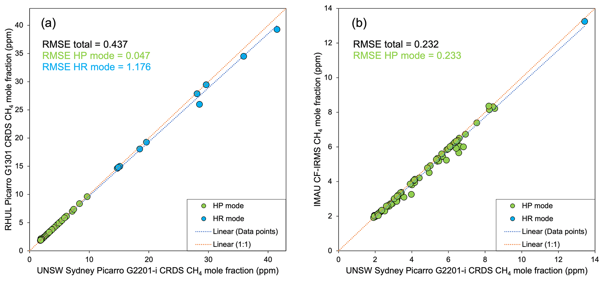
Figure A1Cross-plots of CH4 mole fraction values measured from bag samples using the UNSW Sydney Picarro G2201-i CRDS and the RHUL Picarro G1301 CRDS (a) in 2018 and the UNSW Sydney Picarro G2201-i CRDS and IMAU CF-IRMS (b) in 2019.
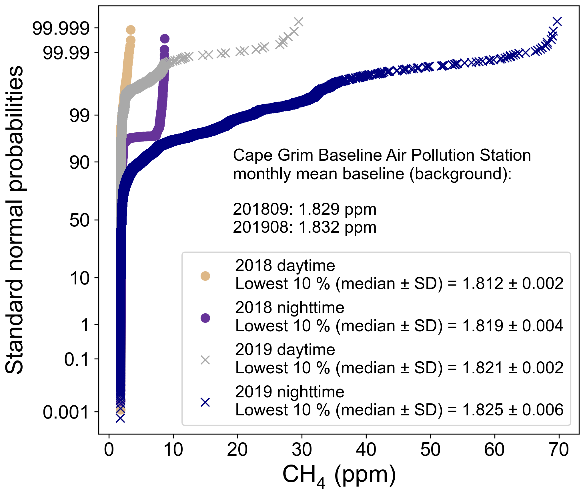
Figure A2Probability of CH4 mole fraction values measured from daytime and nighttime surveys in 2018 and 2019. The median of the lowest 10 %±standard deviation (SD) was calculated to represent the background ambient air.
Each plume set of air samples (blue dots) was analysed using the Keeling plot method. The results are shown in Figs. A3–A7. For each graph the blue line is the Bayesian linear regression posterior mean fit, and the shaded zone is the 95 % Bayesian credible interval.
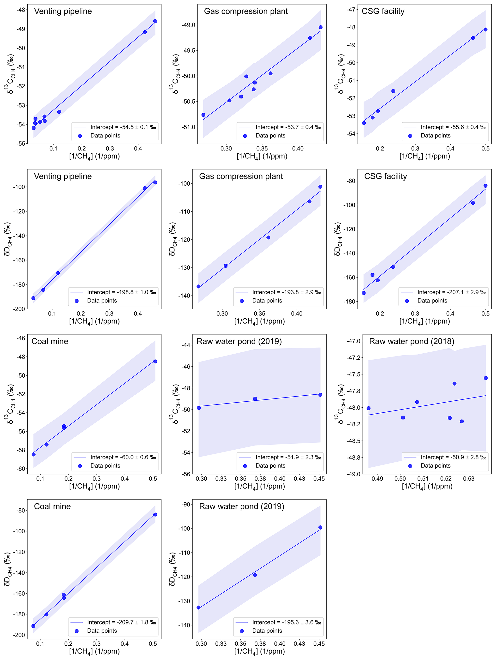
Figure A3Keeling plots of all data from CSG infrastructures and a coal mine analysed using Bayesian linear regression. Upper panels show the results for δ13C and lower panels show the results for δD.
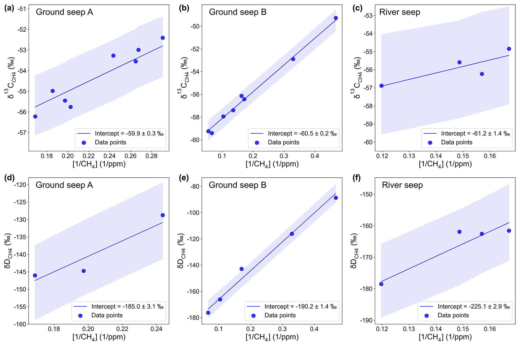
Figure A4Keeling plots of all data from ground and river seeps analysed using Bayesian linear regression. Upper panels show the results for δ13C and lower panels show the results for δD.
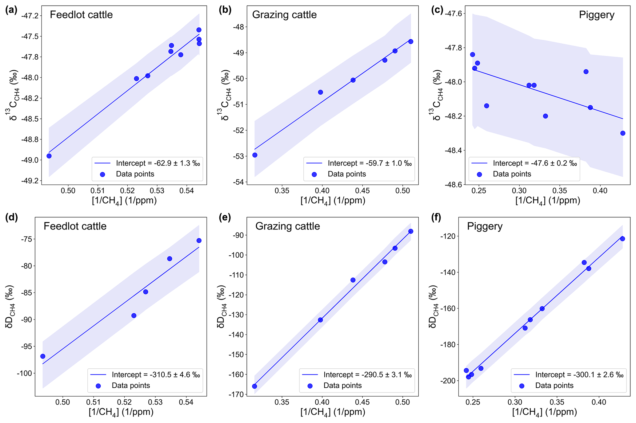
Figure A5Keeling plots of all data from agricultural sources analysed using Bayesian linear regression. Upper panels show the results for δ13C and lower panels show the results for δD.
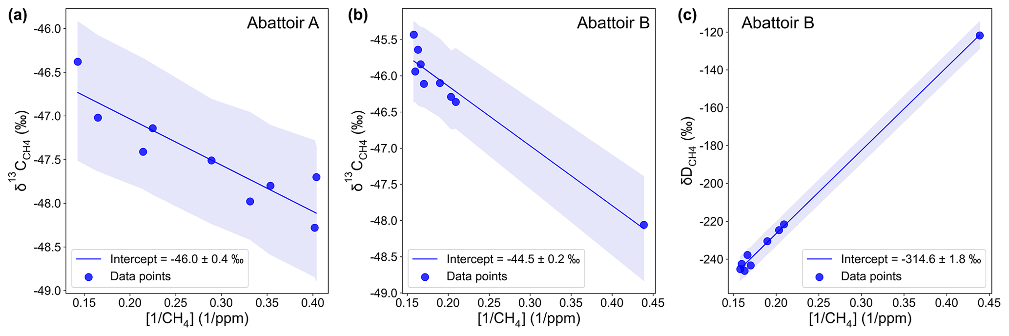
Figure A6Keeling plots of all data from export abattoirs analysed using Bayesian linear regression. Panel (a) (δ13C) shows the result for Abattoir A and panels (b) (δ13C) and (c) (δD) show the results for Abattoir B.

Figure A7Keeling plots of all data from the WWTP and landfill analysed using Bayesian linear regression. Panels (a) (δ13C) and (b) (δD) show the results for WWTP and panel (c) (δ13C) shows the result for landfill.

Figure A8Dependency between the 95 % credible interval range of δ13C (a) and δD (b) derived from the Keeling plot method and number of samples and measured CH4 mole fraction range from the corresponding measured sources.
All data are available from the corresponding author upon request.
BFJK, EGN, REF, JLF, DL and SS conceptualized the project, and BFJK, REF and SS obtained the funding. XL, SJH, SS and BFJK did the fieldwork and sampling investigation. XL, REF, JLF, DL, TR, CvdV and MM undertook the formal laboratory analyses of the air samples. BFJK, XL, REF, JLF and SS developed the methodologies and workflow for analyzing the data. XL did the formal data analyses, wrote the original draft and produced all visualizations under the supervision of BFJK and REF. All the authors contributed to the validation, review and editing of the manuscript. The project was administered by BFJK, REF, TR and SS.
The authors declare that they have no conflict of interest.
Publisher's note: Copernicus Publications remains neutral with regard to jurisdictional claims in published maps and institutional affiliations.
This work was under the support of the Climate and Clean Air Coalition (CCAC) Oil and Gas Methane Science Studies (MSS), hosted by the United Nations Environment Programme. Funding for MSS was provided by the Environmental Defense Fund, Oil and Gas Climate Initiative, European Commission, and CCAC. The authors thank the MSS Science Advisory Committee, the MSS Technical Working Group as well as Christopher Konek for valuable suggestions and comments on this project. We also thank Bruno Neininger and Jorg Hacker for useful inputs during the field campaign. The authors appreciate the insightful feedbacks from the reviewers, which improved the overall quality of the paper.
This research has been supported by the United Nations Environment Programme (grant nos. DTIE18-EN067 and DTIE19-EN0XX, recorded at UNSW Sydney as project nos. RG181430 and RG192900), UNSW–China Scholarship Council (CSC), the European Union's Horizon 2020 research and innovation programme (Marie Sklodowska-Curie grant no. 722479), and the Robertson Foundation.
This paper was edited by Tanja Schuck and reviewed by two anonymous referees.
AGL Energy Limited: Agl Fugitive Methane Emissions Monitoring Campaign-Final Report, 25 pp., avaialble at: https://www.agl.com.au/-/media/aglmedia/documents/about- agl/how-we-source-energy/gloucester/gloucester-document- repository/environmental-reports/20151103_agl-fugitive-methane-emissions-monitoring-campaign—final-report.pdf ?la=en&hash=99169308541465298D02848CFB1EF5C3 (last access: 18 May 2020), 2015.
Allen, G., Hollingsworth, P., Kabbabe, K., Pitt, J. R., Mead, M. I., Illingworth, S., Roberts, G., Bourn, M., Shallcross, D. E., and Percival, C. J.: The development and trial of an unmanned aerial system for the measurement of methane flux from landfill and greenhouse gas emission hotspots, Waste Manage., 87, 883–892, https://doi.org/10.1016/j.wasman.2017.12.024, 2019.
Allen, M. R., Shine, K. P., Fuglestvedt, J. S., Millar, R. J., Cain, M., Frame, D. J., and Macey, A. H.: A solution to the misrepresentations of CO2-equivalent emissions of short-lived climate pollutants under ambitious mitigation, npj Climate and Atmospheric Science, 1, 1–8, https://doi.org/10.1038/s41612-018-0026-8, 2018.
Assan, S., Baudic, A., Guemri, A., Ciais, P., Gros, V., and Vogel, F. R.: Characterization of interferences to in situ observations of δ13CH4 and C2H6 when using a cavity ring-down spectrometer at industrial sites, Atmos. Meas. Tech., 10, 2077–2091, https://doi.org/10.5194/amt-10-2077-2017, 2017.
Assan, S., Vogel, F. R., Gros, V., Baudic, A., Staufer, J., and Ciais, P.: Can we separate industrial CH4 emission sources from atmospheric observations? – A test case for carbon isotopes, PMF and enhanced APCA, Atmos. Environ., 187, 317–327, https://doi.org/10.1016/j.atmosenv.2018.05.004, 2018.
Australian Bureau of Statistics: Agricultural Commodities, Australia, 2018–19 financial year, avaialble at: https://www.abs.gov.au/statistics/industry/agriculture/agricultural-commodities-australia/latest-release#data-download, last access: 16 June 2020.
Australian Competition and Consumer Commission: Gas inquiry 2017–2025 Interim report, 142 pp., avaialble at: https://www.accc.gov.au/system/files/Gas%20inquiry%20-%20January%202020%20interim%20report%20-%20revised.pdf, last access: 18 May 2020.
Australian Government: Geoscape Administrative Boundaries, avaialble at: https://data.gov.au/data/dataset/bdcf5b09-89bc-47ec-9281-6b8e9ee147aa, last access: 10 June 2020.
Auatralian Government: National Greenhouse Gas Inventory – UNFCCC classifications, avaialble at: https://ageis.climatechange.gov.au/UNFCCC.aspx (last access: 16 June 2020), 2019.
Baer, D. S., Paul, J. B., Gupta, M., and O'Keefe, A.: Sensitive absorption measurements in the near-infrared region using off-axis integrated-cavity-output spectroscopy, Appl. Phys. B-Lasers O., 75, 261–265, https://doi.org/10.1007/s00340-002-0971-z, 2002.
Bakkaloglu, S., Lowry, D., Fisher, R. E., France, J. L., Lanoiselle, M., and Fernandez, J.: Characterization and Quantification of Methane Emissions from Waste in the UK, EGU General Assembly 2020, Online, 4–8 May 2020, EGU2020-17839, https://doi.org/10.5194/egusphere-egu2020-17839, 2020.
Baldwin, S. A. and Larson, M. J.: An introduction to using Bayesian linear regression with clinical data, Behav. Res. Ther., 98, 58–75, https://doi.org/10.1016/j.brat.2016.12.016, 2017.
Baublys, K. A., Hamilton, S. K., Golding, S. D., Vink, S., and Esterle, J.: Microbial controls on the origin and evolution of coal seam gases and production waters of the Walloon Subgroup; Surat Basin, Australia, Int. J. Coal Geol., 147–148, 85–104, https://doi.org/10.1016/j.coal.2015.06.007, 2015.
Beck, V., Chen, H., Gerbig, C., Bergamaschi, P., Bruhwiler, L., Houweling, S., Rckmann, T., Kolle, O., Steinbach, J., Koch, T., Sapart, C. J., Van Der Veen, C., Frankenberg, C., Andreae, M. O., Artaxo, P., Longo, K. M., and Wofsy, S. C.: Methane airborne measurements and comparison to global models during BARCA, J. Geophys. Res.-Atmos., 117, D15310, https://doi.org/10.1029/2011JD017345, 2012.
Beef Central: Qld's Grassdale feedlot completes expansion to 75,000 head, available at: https://www.beefcentral.com/lotfeeding/qlds-grassdale-feedlot-completes-expansion-to-75000-head/, last access: 3 September 2020.
Bilek, R. S., Tyler, S. C., Kurihara, M., and Yagi, K.: Investigation of cattle methane production and emission over a 24 h period using measurements of δ13C and δD of emitted CH4 and rumen water, J. Geophys. Res.-Atmos., 106, 15405–15413, https://doi.org/10.1029/2001JD900177, 2001.
Bousquet, P., Ciais, P., Miller, J. B., Dlugokencky, E. J., Hauglustaine, D. A., Prigent, C., Van Der Werf, G. R., Peylin, P., Brunke, E. G., Carouge, C., Langenfelds, R. L., Lathière, J., Papa, F., Ramonet, M., Schmidt, M., Steele, L. P., Tyler, S. C., and White, J.: Contribution of anthropogenic and natural sources to atmospheric methane variability, Nature, 443, 439–443, https://doi.org/10.1038/nature05132, 2006.
BP: BP Statistical Review of World Energy 2019, 61 pp., available at: https://www.bp.com/content/dam/bp/business-sites/en/global/corporate/pdfs/energy-economics/statistical-review/bp-stats-review-2019-full-report.pdf (last access: 18 May 2020), 2019.
Brandt, A. R., Heath, G. A., and Cooley, D.: Methane Leaks from Natural Gas Systems Follow Extreme Distributions, Environ. Sci. Technol., 50, 12512–12520, https://doi.org/10.1021/acs.est.6b04303, 2016.
Brass, M. and Röckmann, T.: Continuous-flow isotope ratio mass spectrometry method for carbon and hydrogen isotope measurements on atmospheric methane, Atmos. Meas. Tech., 3, 1707–1721, https://doi.org/10.5194/amt-3-1707-2010, 2010.
Brownlow, R., Lowry, D., Fisher, R. E., France, J. L., Lanoisellé, M., White, B., Wooster, M. J., Zhang, T., and Nisbet, E. G.: Isotopic Ratios of Tropical Methane Emissions by Atmospheric Measurement, Global Biogeochem. Cy., 31, 1408–1419, https://doi.org/10.1002/2017GB005689, 2017.
Chandra, N., Patra, P. K., Bisht, J. S. H., Ito, A., Umezawa, T., Saigusa, N., Morimoto, S., Aoki, S., Janssens–Maenhout, G., FUJITA, R., Takigawa, M., Watanabe, S., Saitoh, N., and Canadell, J. G.: Emissions from the Oil and Gas Sectors, Coal Mining and Ruminant Farming Drive Methane Growth over the Past Three Decades, J. Meteorol. Soc. Jpn. Ser. II, 99, 309–337, https://doi.org/10.2151/jmsj.2021-015, 2021.
Conley, S., Franco, G., Faloona, I., Blake, D. R., Peischl, J., and Ryerson, T. B.: Methane emissions from the 2015 Aliso Canyon blowout in Los Angeles, CA, Science, 351, 1317–1320, https://doi.org/10.1126/science.aaf2348, 2016.
Day, C., Tibbett, S., Sestak, A., Knight, S., Marvig, C., Mcgarry, P., Weir, S., White, S., Armand, S., Van Holst, S., Fry, J., Dell'amico, R., Halliburton, M., and Azzi, B.: Methane and Volatile Organic Compound Emissions in New South Wales, CSIRO, Australia, 312 pp., available at: https://www.epa.nsw.gov.au/~/media/EPA/Corporate%20Site/resources/air/methane-volatile-organic-compound-emissions-nsw-3063.ashx (last access: 18 May 2020), 2016.
Day, S., Dell'amico, M., Etheridge, D., Ong, C., Rodger, A., Sherman, B., and Barrett, D. J.: Characterisation of Regional Fluxes of Methane in the Surat Basin, Queensland. Phase 1: A Review and Analysis of Literature on Methane Detection and Flux Determination, Australia, CSIRO, Australia, 57 pp., available at: https://gisera.csiro.au/wp-content/uploads/2018/03/GHG-1-Literature-review.pdf (last access: 18 May 2020), 2013.
Day, S., Dell'Amico, M., Fry, R., and Tousi, H.: Field Measurements of Fugitive Emissions from Equipment and Well Casings in Australian Coal Seam Gas Production Facilities, CSIRO, Australia, 41 pp., available at: https://www.aph.gov.au/DocumentStore.ashx?id=f8ee0ca1-08c6-497e-a265-4896a1e80bc0&subId=410955 (last access: 18 May 2020), 2014.
Day, S., Ong, C., Rodger, A., Etheridge, D., Hibberd, M., Van Gorsel, E., Spencer, D., Krummel, P., Zegelin, S., Fry, R., Dell'amico, M., Sestak, S., Williams, D., Zoë, L., and Barrett, D.: Characterisation of Regional Fluxes of Methane in the Surat Basin, Queensland. Phase 2: A pilot study of methodology to detect and quantify methane sources, Australia, CSIRO, Australia, 76 pp., available at: https://www.researchgate.net/publication/280317211_Characterisation_of_Regional_Fluxes_of_Methane_in_the_Surat_Basin_Queensland (last access: 18 May 2020), 2015.
Department of Natural Resources and Mines: Summary technical report – Part 1: Condamine River gas seep investigation, 35 pp., available at: https://www.daf.qld.gov.au/__data/assets/pdf_file/0004/1448896/15-002.pdf (last access: 18 May 2020), 2012.
Dlugokencky, E. J.: Annual Increase in Globally-Averaged Atmospheric Methane, NOAA/GML, available at: https://www.esrl.noaa.gov/gmd/ccgg/trends_ch4/, last access: 15 February 2021.
Dlugokencky, E. J., Myers, R. C., Lang, P. M., Masarie, K. A., Crotwell, A. M., Thoning, K. W., Hall, B. D., Elkins, J. W., and Steele, L. P.: Conversion of NOAA atmospheric dry air CH4 mole fractions to a gravimetrically prepared standard scale, J. Geophys. Res.-Atmos., 110, 1–8, https://doi.org/10.1029/2005JD006035, 2005.
Dlugokencky, E. J., Nisbet, E. G., Fisher, R., and Lowry, D.: Global atmospheric methane: Budget, changes and dangers, Philos. T. R. Soc. A., 369, 2058–2072, https://doi.org/10.1098/rsta.2010.0341, 2011.
DNV GL: Energy Transition Outlook 2019 Oil and Gas, 95 pp., available at: https://eto.dnv.com/2019/#ETO2019-top (last access: 18 May 2020), 2019.
Doig, A. and Stanmore, P.: The Clarence-Moreton Basin in New South Wales; geology, stratigraphy and coal seam gas characteristics, in: Eastern Australasian Basins Symposium IV, Brisbane, QLD, Australia, 10–14 September 2012, 1–14, available at: https://www.researchgate.net/publication/285769720_The_Clarence-Moreton_Basin_in_New_South_Wales_geology_stratigraphy_and_coal_seam_gas_characteristics (last access: 18 May 2020), 2012.
Draper, J. J. and Boreham, C. J.: Geological Controls On Exploitable Coal Seam Gas Distribution In Queensland, Journal of the Australian Petroleum Production and Exploration Association, 46, 366, https://doi.org/10.1071/aj05019, 2006.
EIA: Shale gas production drives world natural gas production growth, available at: https://www.eia.gov/todayinenergy/detail.php?id=27512 (last access: 18 May 2020), 2016.
Etiope, G., Ciotoli, G., Schwietzke, S., and Schoell, M.: Gridded maps of geological methane emissions and their isotopic signature, Earth Syst. Sci. Data, 11, 1–22, https://doi.org/10.5194/essd-11-1-2019, 2019.
Etminan, M., Myhre, G., Highwood, E. J., and Shine, K. P.: Radiative forcing of carbon dioxide, methane, and nitrous oxide: A significant revision of the methane radiative forcing, Geophys. Res. Lett., 43, 12614–12623, https://doi.org/10.1002/2016GL071930, 2016.
Eyer, S., Tuzson, B., Popa, M. E., van der Veen, C., Röckmann, T., Rothe, M., Brand, W. A., Fisher, R., Lowry, D., Nisbet, E. G., Brennwald, M. S., Harris, E., Zellweger, C., Emmenegger, L., Fischer, H., and Mohn, J.: Real-time analysis of δ13C- and δD−CH4 in ambient air with laser spectroscopy: method development and first intercomparison results, Atmos. Meas. Tech., 9, 263–280, https://doi.org/10.5194/amt-9-263-2016, 2016.
Feinberg, A. I., Coulon, A., Stenke, A., Schwietzke, S., and Peter, T.: Isotopic source signatures: Impact of regional variability on the δ13CH4 trend and spatial distribution, Atmos. Environ., 174, 99–111, https://doi.org/10.1016/j.atmosenv.2017.11.037, 2018.
Fisher, R., Lowry, D., Wilkin, O., Sriskantharajah, S., and Nisbet, E. G.: High-precision, automated stable isotope analysis of atmospheric methane and carbon dioxide using continuous-flow isotope-ratio mass spectrometry, Rapid Commun. Mass Sp., 20, 200–208, https://doi.org/10.1002/rcm.2300, 2006.
Fisher, R. E., Sriskantharajah, S., Lowry, D., Lanoisellé, M., Fowler, C. M. R., James, R. H., Hermansen, O., Lund Myhre, C., Stohl, A., Greinert, J., Nisbet-Jones, P. B. R., Mienert, J., and Nisbet, E. G.: Arctic methane sources: Isotopic evidence for atmospheric inputs, Geophys. Res. Lett., 38, L21803, https://doi.org/10.1029/2011GL049319, 2011.
Fisher, R. E., France, J. L., Lowry, D., Lanoisellé, M., Brownlow, R., Pyle, J. A., Cain, M., Warwick, N., Skiba, U. M., Drewer, J., Dinsmore, K. J., Leeson, S. R., Bauguitte, S. J. -B., Wellpott, A., O'Shea, S. J., Allen, G., Gallagher, M. W., Pitt, J., Percival, C. J., Bower, K., George, C., Hayman, G. D., Aalto, T., Lohila, A., Aurela, M., Laurila, T., Crill, P. M., McCalley, C. K., and Nisbet, E. G.: Measurement of the 13C isotopic signature of methane emissions from northern European wetlands, Global Biogeochem. Cy., 31, 605–623, https://doi.org/10.1002/2016GB005504, 2017.
Flesch, T. K., C Vergé, X. P., Desjardins, R. L., and Worth, D.: Methane emissions from a swine manure tank in western Canada, Can. J. Anim. Sci., 93, 159–169, https://doi.org/10.4141/CJAS2012-072, 2013.
France, J. L., Cain, M., Fisher, R. E., Lowry, D., Allen, G., O'Shea, S. J., Illingworth, S., Pyle, J., Warwick, N., Jones, B. T., Gallagher, M. W., Bower, K., Le Breton, M., Percival, C., Muller, J., Welpott, A., Bauguitte, S., George, C., Hayman, G. D., Manning, A. J., Myhre, C. L., Lanoisellé, M., and Nisbet, E. G.: Measurements of δ13C in CH4 and using particle dispersion modeling to characterize sources of Arctic methane within an air mass, J. Geophys. Res.-Atmos., 121, 14257–14270, https://doi.org/10.1002/2016JD026006, 2016.
Fries, A. E., Schifman, L. A., Shuster, W. D., and Townsend-Small, A.: Street-level emissions of methane and nitrous oxide from the wastewater collection system in Cincinnati, Ohio, Environ. Pollut., 236, 247–256, https://doi.org/10.1016/j.envpol.2018.01.076, 2018.
Ganesan, A. L., Schwietzke, S., Poulter, B., Arnold, T., Lan, X., Rigby, M., Vogel, F. R., van der Werf, G. R., Janssens-Maenhout, G., Boesch, H., Pandey, S., Manning, A. J., Jackson, R. B., Nisbet, E. G., and Manning, M. R.: Advancing Scientific Understanding of the Global Methane Budget in Support of the Paris Agreement, Global Biogeochem. Cy., 33, 1475–1512, https://doi.org/10.1029/2018GB006065, 2019.
Ginty, E. M.: Carbon Isotopic Evidence That Coal Derived Methane Is Altering The Chemistry of The Global Atmosphere, Bachelor's degree (Honors) thesis, The University of New South Wales, Sydney, Australia, 63 pp., 2016.
Golding, S. D., Uysal, I. T., Bolhar, R., Boreham, C. J., Dawson, G. K. W., Baublys, K. A., and Esterle, J. S.: Carbon dioxide-rich coals of the Oaky Creek area, central Bowen Basin: a natural analogue for carbon sequestration in coal systems, Aust. J. Earth Sci., 60, 125–140, https://doi.org/10.1080/08120099.2012.750627, 2013.
Hamilton, S. K., Esterle, J. S., and Golding, S. D.: Geological interpretation of gas content trends, Walloon Subgroup, eastern Surat Basin, Queensland, Australia, Int. J. Coal Geol., 101, 21–35, https://doi.org/10.1016/j.coal.2012.07.001, 2012.
Hamilton, S. K., Golding, S. D., Baublys, K. A., and Esterle, J. S.: Stable isotopic and molecular composition of desorbed coal seam gases from the Walloon Subgroup, eastern Surat Basin, Australia, Int. J. Coal Geol., 122, 21–36, https://doi.org/10.1016/j.coal.2013.12.003, 2014.
Hamilton, S. K., Golding, S. D., Baublys, K. A., and Esterle, J. S.: Conceptual exploration targeting for microbially enhanced coal bed methane (MECoM) in the Walloon Subgroup, eastern Surat Basin, Australia, Int. J. Coal Geol., 138, 68–82, https://doi.org/10.1016/j.coal.2014.12.002, 2015.
Hatch, M. A., Kennedy, M. J., Hamilton, M. W., and Vincent, R. A.: Methane variability associated with natural and anthropogenic sources in an Australian context, Aust. J. Earth Sci., 65, 683–690, https://doi.org/10.1080/08120099.2018.1471004, 2018.
Hemisphere GNSS: http://www.ses-services.com/images/Atlas_Brochure_06.2015_WEB.pdf, (last access: 18 May 2020), 2015.
Hmiel, B., Petrenko, V. V., Dyonisius, M. N., Buizert, C., Smith, A. M., Place, P. F., Harth, C., Beaudette, R., Hua, Q., Yang, B., Vimont, I., Michel, S. E., Severinghaus, J. P., Etheridge, D., Bromley, T., Schmitt, J., Faïn, X., Weiss, R. F., and Dlugokencky, E.: Preindustrial 14CH4 indicates greater anthropogenic fossil CH4 emissions, Nature, 578, 409–412, https://doi.org/10.1038/s41586-020-1991-8, 2020.
Hoheisel, A., Yeman, C., Dinger, F., Eckhardt, H., and Schmidt, M.: An improved method for mobile characterisation of δ13CH4 source signatures and its application in Germany, Atmos. Meas. Tech., 12, 1123–1139, https://doi.org/10.5194/amt-12-1123-2019, 2019.
IEA: Key World Energy Statistics, available at: https://www.iea.org/reports/key-world-energy-statistics-2019 (last access: 18 May 2020), 2019.
IEA: Methane Tracker Database, available at: https://www.iea.org/articles/methane-tracker-database, last access: 8 April 2021.
Iverach, C. P., Lowry, D., France, J. L., Fisher, R. E., Nisbet, E. G., Baker, A., Acworth, R. I., Loh, Z., Day, S., and Kelly, B. F. J.: The Complexities of Continuous Air Monitoring in Attributing Methane to Sources of Production, Australian Earth Science Convention 2014, 7–10 July 2014, Newcastle, Australia, 01EGF-04, 2014.
Iverach, C. P., Cendón, D. I., Hankin, S. I., Lowry, D., Fisher, R. E., France, J. L., Nisbet, E. G., Baker, A., and Kelly, B. F. J.: Assessing Connectivity Between an Overlying Aquifer and a Coal Seam Gas Resource Using Methane Isotopes, Dissolved Organic Carbon and Tritium, Sci. Rep., 5, 1–11, https://doi.org/10.1038/srep15996, 2015.
Iverach, C. P., Beckmann, S., Cendón, D. I., Manefield, M., and Kelly, B. F. J.: Biogeochemical constraints on the origin of methane in an alluvial aquifer: evidence for the upward migration of methane from underlying coal measures, Biogeosciences, 14, 215–228, https://doi.org/10.5194/bg-14-215-2017, 2017.
Jackson, R. B., Saunois, M., Bousquet, P., Canadell, J. G., Poulter, B., Stavert, A. R., Bergamaschi, P., Niwa, Y., Segers, A., and Tsuruta, A.: Increasing anthropogenic methane emissions arise equally from agricultural and fossil fuel sources, Environ. Res. Lett., 15, 071002, https://doi.org/10.1088/1748-9326/ab9ed2, 2020.
Jaynes, E. T.: Straight Line Fitting – A Bayesian Solution, available at: https://bayes.wustl.edu/etj/articles/leapz.pdf (last access: 30 June 2021), 1999.
Joos, F., Roth, R., Fuglestvedt, J. S., Peters, G. P., Enting, I. G., von Bloh, W., Brovkin, V., Burke, E. J., Eby, M., Edwards, N. R., Friedrich, T., Frölicher, T. L., Halloran, P. R., Holden, P. B., Jones, C., Kleinen, T., Mackenzie, F. T., Matsumoto, K., Meinshausen, M., Plattner, G.-K., Reisinger, A., Segschneider, J., Shaffer, G., Steinacher, M., Strassmann, K., Tanaka, K., Timmermann, A., and Weaver, A. J.: Carbon dioxide and climate impulse response functions for the computation of greenhouse gas metrics: a multi-model analysis, Atmos. Chem. Phys., 13, 2793–2825, https://doi.org/10.5194/acp-13-2793-2013, 2013.
Keeling, C. D.: The concentration and isotopic abundances of atmospheric carbon dioxide in rural areas, Geochim. Cosmochim. Ac., 13, 322–334, https://doi.org/10.1016/0016-7037(58)90033-4, 1958.
Kelly, B. F. J. and Fisher, R. E.: Continuous Tracking of Air Parcel Mixing Using Discrete Wavelet Transformation of Urban Ground Level Atmospheric Methane Measurements, in: Geophysical Research Abstracts, 20, EGU2018-6265–1, available at: https://meetingorganizer.copernicus.org/EGU2018/EGU2018-6265-1.pdf (last access: 18 May 2020), 2018.
Kelly, B. F. J. and Iverach, C. P.: River on fire: even if it's not coal seam gas we should still be concerned, The Conversation, 3 May, available at: https://theconversation.com/river-on-fire-even-if-its-not-coal-seam-gas-we-should-still-be-concerned-58718 (last access: 27 May 2020), 2016.
Kelly, B. F. J., Iverach, C. P., Lowry, D., Fisher, R. E., France, J. L., and Nisbet, E. G.: Fugitive methane emissions from natural, urban, agricultural, and energy-production landscapes of eastern Australia, Geophysical Research Abstracts, 17, EGU2015–5135, available at: https://meetingorganizer.copernicus.org/EGU2015/EGU2015-5135.pdf (last access: 18 May 2020), 2015.
Kelly, B. F. J., Iverach, C. P., Ginty, E., Bashir, S., Lowry, D., Fisher, R. E., France, J. L., and Nisbet, E. G.: The case for refining bottom-up methane emission inventories using top-down measurements, Geophysical Research Abstracts, 19, EGU2017-5700, available at: https://meetingorganizer.copernicus.org/EGU2017/EGU2017-5700.pdf (last access: 18 May 2020), 2017.
Kille, N., Chiu, R., Frey, M., Hase, F., Sha, M. K., Blumenstock, T., Hannigan, J. W., Orphal, J., Bon, D., and Volkamer, R.: Separation of Methane Emissions From Agricultural and Natural Gas Sources in the Colorado Front Range, Geophys. Res. Lett., 46, 3990–3998, https://doi.org/10.1029/2019GL082132, 2019.
Kirschke, S., Bousquet, P., Ciais, P., Saunois, M., Canadell, J. G., Dlugokencky, E. J., Bergamaschi, P., Bergmann, D., Blake, D. R., Bruhwiler, L., Cameron-Smith, P., Castaldi, S., Chevallier, F., Feng, L., Fraser, A., Heimann, M., Hodson, E. L., Houweling, S., Josse, B., Fraser, P. J., Krummel, P. B., Lamarque, J.-F., Langenfelds, R. L., Le Quéré, C., Naik, V., Palmer, P. I., Pison, I., Plummer, D., Poulter, B., Prinn, R. G., Rigby, M., Ringeval, B., Santini, M., Schmidt, M., Shindell, D. T., Simpson, I. J., Spahni, R., Paul Steele, L., Strode, S. A., Sudo, K., Szopa, S., van der Werf, G. R., Voulgarakis, A., van Weele, M., Weiss, R. F., Williams, J. E., and Zeng, G.: Three decades of global methane sources and sinks, Nat. Geosci., 6, 813–823, https://doi.org/10.1038/NGEO1955, 2013.
Lan, X., Tans, P., Sweeney, C., Andrews, A., Dlugokencky, E., Schwietzke, S., Kofler, J., McKain, K., Thoning, K., Crotwell, M., Montzka, S., Miller, B. R., and Biraud, S. C.: Long-Term Measurements Show Little Evidence for Large Increases in Total U.S. Methane Emissions Over the Past Decade, Geophys. Res. Lett., 46, 4991–4999, https://doi.org/10.1029/2018GL081731, 2019.
Levin, I., Bergamaschi, P., Dörr, H., and Trapp, D.: Stable isotopic signature of methane from major sources in Germany, Chemosphere, 26, 161–177, https://doi.org/10.1016/0045-6535(93)90419-6, 1993.
Lowry, D., Fisher, R. E., France, J. L., Coleman, M., Lanoisellé, M., Zazzeri, G., Nisbet, E. G., Shaw, J. T., Allen, G., Pitt, J., and Ward, R. S.: Environmental baseline monitoring for shale gas development in the UK: Identification and geochemical characterisation of local source emissions of methane to atmosphere, Sci. Total Environ., 708, 134600, https://doi.org/10.1016/j.scitotenv.2019.134600, 2020.
Lu, X., Iverach, C. P., Harris, S. J., Fisher, R. E., Lowry, D., France, J. L., Nisbet, E. G., Loh, Z. M., Phillips, F., Schwietzke, S., Hacker, J., Neininger, B., and Kelly, B. F. J.: In Plume Miller-Tans Time Series Analyses for Improved Isotopic Source Signature Characterisation, Geophysical Research Abstracts, 21, EGU2019-11559–1, available at: https://meetingorganizer.copernicus.org/EGU2019/EGU2019-11559-1.pdf (last access: 18 May 2020), 2019.
Lu, X., Harris, S. J., Fisher, R. E., Lowry, D., France, J. L., Hacker, J., Neininger, B., Röckmann, T., van der Veen, C., Menoud, M., Schwietzke, S., and Kelly, B. F. J.: Methane Source Attribution Challenges in the Surat Basin, Australia, EGU General Assembly 2020, Online, 4–8 May 2020, EGU2020-12508, https://doi.org/10.5194/egusphere-egu2020-12508, 2020.
Luhar, A., Etheridge, D., Loh, Z., Noonan, N., Spencer, D., and Day, S.: Characterisation of Regional Fluxes of Methane in the Surat Basin, Queensland. Final report on Task 3: Broad scale application of methane detection, and Task 4: Methane emissions enhanced modelling, Report to the Gas Industry Social and Environmental Research Alliance (GISERA), CSIRO Australia, Report no. EP185211, 98 pp., https://publications.csiro.au/rpr/pub?pid=csiro:EP185211, 2018.
Luhar, A. K., Etheridge, D. M., Loh, Z. M., Noonan, J., Spencer, D., Smith, L., and Ong, C.: Quantifying methane emissions from Queensland's coal seam gas producing Surat Basin using inventory data and a regional Bayesian inversion, Atmos. Chem. Phys., 20, 15487–15511, https://doi.org/10.5194/acp-20-15487-2020, 2020.
Maazallahi, H., Fernandez, J. M., Menoud, M., Zavala-Araiza, D., Weller, Z. D., Schwietzke, S., von Fischer, J. C., Denier van der Gon, H., and Röckmann, T.: Methane mapping, emission quantification, and attribution in two European cities: Utrecht (NL) and Hamburg (DE), Atmos. Chem. Phys., 20, 14717–14740, https://doi.org/10.5194/acp-20-14717-2020, 2020.
Maher, D. T., Santos, I. R., and Tait, D. R.: Mapping methane and carbon dioxide concentrations and δ13C values in the atmosphere of two Australian coal seam gas fields, Water Air Soil Poll., 225, 1–9, https://doi.org/10.1007/s11270-014-2216-2, 2014.
Maher, D. T., Cowley, K., Santos, I. R., Macklin, P., and Eyre, B. D.: Methane and carbon dioxide dynamics in a subtropical estuary over a diel cycle: Insights from automated in situ radioactive and stable isotope measurements, Mar. Chem., 168, 69–79, https://doi.org/10.1016/j.marchem.2014.10.017, 2015.
McGinn, S. M., Chen, D., Loh, Z., Hill, J., Beauchemin, K. A., and Denmead, O. T.: Methane emissions from feedlot cattle in Australia and Canada, Aust. J. Exp. Agr., 48, 183, https://doi.org/10.1071/EA07204, 2008.
McGlade, C., Speirs, J., and Sorrell, S.: Unconventional gas – A review of regional and global resource estimates, Energy, 55, 571–584, https://doi.org/10.1016/j.energy.2013.01.048, 2013.
McNorton, J., Wilson, C., Gloor, M., Parker, R. J., Boesch, H., Feng, W., Hossaini, R., and Chipperfield, M. P.: Attribution of recent increases in atmospheric methane through 3-D inverse modelling, Atmos. Chem. Phys., 18, 18149–18168, https://doi.org/10.5194/acp-18-18149-2018, 2018.
Menoud, M., van der Veen, C., Scheeren, B., Chen, H., Szénási, B., Morales, R. P., Pison, I., Bousquet, P., Brunner, D., and Röckmann, T.: Characterisation of methane sources in Lutjewad, the Netherlands, using quasi-continuous isotopic composition measurements, Tellus B, 72, 1–19, https://doi.org/10.1080/16000889.2020.1823733, 2020.
Mielke-Maday, I., Schwietzke, S., Yacovitch, T., Miller, B., Conley, S., Kofler, J., Handley, P., Thorley, E., Herndon, S. C., Hall, B., Dlugokencky, E., Lang, P., Wolter, S., Moglia, E., Crotwell, M., Crotwell, A., Rhodes, M., Kitzis, D., Vaughn, T., Bell, C., Zimmerle, D., Schnell, R., and Pétron, G.: Methane source attribution in a U.S. dry gas basin using spatial patterns of ground and airborne ethane and methane measurements, Elementa, 7, 13, https://doi.org/10.1525/elementa.351, 2019.
Milkov, A. V. and Etiope, G.: Revised genetic diagrams for natural gases based on a global dataset of samples, Org. Geochem., 125, 109–120, https://doi.org/10.1016/j.orggeochem.2018.09.002, 2018.
Miller, J. B. and Tans, P. P.: Calculating isotopic fractionation from atmospheric measurements at various scales, Tellus B, 55, 207–214, https://doi.org/10.1034/j.1600-0889.2003.00020.x, 2003.
Monteny, G. J., Bannink, A., and Chadwick, D.: Greenhouse gas abatement strategies for animal husbandry, Agr. Ecosyst. Environ., 112, 163–170, https://doi.org/10.1016/j.agee.2005.08.015, 2006.
Myhre, G., Shindell, D., Bréon F.-M., Collins, W., Fuglestvedt, J., Huang, J., Koch, D., Lamarque, J.-F., Lee, D., Mendoza, B., Nakajima, T., Robock, A., Stephens, G., Takemura, T., and H.Zhang: Anthropogenic and natural radiative forcing, in: Climate Change 2013 the Physical Science Basis: Working Group I Contribution to the Fifth Assessment Report of the Intergovernmental Panel on Climate Change, 9781107057, edited by: Intergovernmental Panel on Climate Change, Cambridge University Press, Cambridge, United Kingdom and New York, NY, USA, 659–740, https://doi.org/10.1017/CBO9781107415324.018, 2013.
Neininger, B. G., Kelly, B. F. J., Hacker, J. M., Lu, X., and Schwietzke, S.: Coal seam gas industry methane emissions in the Surat Basin, Australia: Comparing airborne measurements with inventories, Philos. T. R. Soc. A., accepted, 2021.
NH Foods: Oakey Beef Exports, available at: https://www.nh-foods.com.au/facilities/oakey-beef-exports/, last access: 4 September 2020.
Nisbet, E. G., Dlugokencky, E. J., and Bousquet, P.: Methane on the rise – Again, Science, 343, 493–495, https://doi.org/10.1126/science.1247828, 2014.
Nisbet, E. G., Dlugokencky, E. J., Manning, M. R., Lowry, D., Fisher, R. E., France, J. L., Michel, S. E., Miller, J. B., White, J. W. C., Vaughn, B., Bousquet, P., Pyle, J. A., Warwick, N. J., Cain, M., Brownlow, R., Zazzeri, G., Lanoisellé, M., Manning, A. C., Gloor, E., Worthy, D. E. J., Brunke, E.-G., Labuschagne, C., Wolff, E. W., and Ganesan, A. L.: Rising atmospheric methane: 2007–2014 growth and isotopic shift, Global Biogeochem. Cy., 30, 1356–1370, https://doi.org/10.1002/2016GB005406, 2016.
Nisbet, E. G., Manning, M. R., Dlugokencky, E. J., Fisher, R. E., Lowry, D., Michel, S. E., Myhre, C. L., Platt, S. M., Allen, G., Bousquet, P., Brownlow, R., Cain, M., France, J. L., Hermansen, O., Hossaini, R., Jones, A. E., Levin, I., Manning, A. C., Myhre, G., Pyle, J. A., Vaughn, B. H., Warwick, N. J., and White, J. W. C.: Very Strong Atmospheric Methane Growth in the 4 Years 2014–2017: Implications for the Paris Agreement, Global Biogeochem. Cy., 33, 318–342, https://doi.org/10.1029/2018GB006009, 2019.
Nisbet, E. G., Fisher, R. E., Lowry, D., France, J. L., Allen, G., Bakkaloglu, S., Broderick, T. J., Cain, M., Coleman, M., Fernandez, J., Forster, G., Griffiths, P. T., Iverach, C. P., Kelly, B. F. J., Manning, M. R., Nisbet-Jones, P. B. R., Pyle, J. A., Townsend-Small, A., al-Shalaan, A., Warwick, N., and Zazzeri, G.: Methane Mitigation: Methods to Reduce Emissions, on the Path to the Paris Agreement, Rev. Geophys., 58, e2019RG000675, https://doi.org/10.1029/2019RG000675, 2020.
Obersky, L., Rafiee, R., Cabral, A. R., Golding, S. D., and Clarke, W. P.: Methodology to determine the extent of anaerobic digestion, composting and CH4 oxidation in a landfill environment, Waste Manage., 76, 364–373, https://doi.org/10.1016/j.wasman.2018.02.029, 2018.
Owen, D. D. R., Shouakar-Stash, O., Morgenstern, U., and Aravena, R.: Thermodynamic and hydrochemical controls on CH4 in a coal seam gas and overlying alluvial aquifer: New insights into CH4 origins, Sci. Rep., 6, 1–20, https://doi.org/10.1038/srep32407, 2016.
Pachauri, R. K., Allen, M. R., Barros, V. R., Broome, J., Cramer, W., Christ, R., Church, J. A., Clarke, L., Dahe, Q., Dasgupta, P., Dubash, N. K., Edenhofer, O., Elgizouli, I., Field, C. B., Forster, P., Friedlingstein, P., Fuglestvedt, J., Gomez-Echeverri, L., Hallegatte, S., Hegerl, G., Howden, M., Jiang, K., Jimenez Cisneroz, B., Kattsov, V., Lee, H., Mach, K. J., Marotzke, J., Mastrandrea, M. D., Meyer, L., Minx, J., Mulugetta, Y., O'Brien, K., Oppenheimer, M., Pereira, J. J., Pichs-Madruga, R., Plattner, G. K., Pörtner, H. O., Power, S. B., Preston, B., Ravindranath, N. H., Reisinger, A., Riahi, K., Rusticucci, M., Scholes, R., Seyboth, K., Sokona, Y., Stavins, R., Stocker, T. F., Tschakert, P., van Vuuren, D. and van Ypserle, J. P., Pachauri R. K., and Meyer L. A. (Eds.): Climate Change 2014: Synthesis Report. Contribution of Working Groups I, II and III to the Fifth Assessment Report of the Intergovernmental Panel on Climate Change, IPCC, Geneva, Switzerland, 151 pp., available at: https://epic.awi.de/id/eprint/37530/ (last access: 30 June 2021), 2014.
Pallasser, R. and Stalker, L.: Dissolved Gas Measurements For Bores In The South Eastern Part Of The Surat Basin (Great Artesian Basin, North Eastern NSW). A report to the NSW Department of Mineral Resources, CSIRO Australia, 18 pp., available at: https://publications.csiro.au/rpr/download?pid=procite:dffbf1b4-9b7e-454b-a0f1-1b75ce01a836&dsid=DS1 (last access: 18 May 2020), 2001.
Pataki, D. E., Ehleringer, J. R., Flanagan, L. B., Yakir, D., Bowling, D. R., Still, C. J., Buchmann, N., Kaplan, J. O., and Berry, J. A.: The application and interpretation of Keeling plots in terrestrial carbon cycle research, Global Biogeochem. Cy., 17, 1022, https://doi.org/10.1029/2001GB001850, 2003.
QGC: QGC Stage 3 Water Monitoring and Management Plan. Chapter 14.0: Associated water management, Queensland Gas Company, 236–256, available at: https://www.shell.com.au/about-us/projects-and-locations/qgc/environment/water-management/reports/_jcr_content/par/expandablelist_48b1/expandablesection_ea.stream/1498083770743/5d3c60df4680077259c49a3dce487c409beab3d0/qgc-stage-3-wmmp-dec-13-14.pdf (last access: 18 May 2020), 2014.
Queensland Government: Queensland Spatial Catalogue – QSpatial, available at: http://qldspatial.information.qld.gov.au/catalogue/custom/detail.page?fid=%7BB443A9EE-861C-46BC-AE7C-D2E023E477EA%7D (last access: 3 September 2020), 2018a.
Queensland Government: Queensland Spatial Catalogue – Qspatial, available at: http://qldspatial.information.qld.gov.au/catalogue/custom/detail.page?fid=%7B30B884DA-4B6C-4129-9081-32525DA3143C%7D (last access: 3 September 2020), 2018b.
Queensland Government: Open Data Portal, Coal industry review statistical tables – Production of saleable coal by individual mines, available at: https://www.data.qld.gov.au/dataset/coal-industry-review-statistical-tables/resource/1b7fb643-c880-42bf-940b-fc3c582d239d (last access: 26 May 2020), 2019.
Queensland Government: Open Data Portal, Queensland borehole series – All bore hole and well locations, available at: https://www.data.qld.gov.au/dataset/queensland-borehole-series/resource/8622f045-628d-4f9b-9be8-df65fb9e5ce0, last access: 26 May 2020a.
Queensland Government: Petroleum and gas production and reserve statistics, available at: https://www.data.qld.gov.au/dataset/petroleum-gas-production-and-reserve-statistics, last access: 16 June 2020b.
Queensland Government: Queensland Globe, available at: https://www.business.qld.gov.au/running-business/support-assistance/mapping-data-imagery/queensland-globe, last access: 22 June 2020c.
Rella, C. W., Hoffnagle, J., He, Y., and Tajima, S.: Local- and regional-scale measurements of CH4, δ13CH4, and C2H6 in the Uintah Basin using a mobile stable isotope analyzer, Atmos. Meas. Tech., 8, 4539–4559, https://doi.org/10.5194/amt-8-4539-2015, 2015.
Rice, A. L., Butenhoff, C. L., Teama, D. G., Röger, F. H., Khalil, M. A. K., and Rasmussen, R. A.: Atmospheric methane isotopic record favors fossil sources flat in 1980s and 1990s with recent increase, Proc. Natl. Acad. Sci. USA, 113, 10791–10796, https://doi.org/10.1073/pnas.1522923113, 2016.
Rigby, M., Montzka, S. A., Prinn, R. G., White, J. W. C., Young, D., O'Doherty, S., Lunt, M. F., Ganesan, A. L., Manning, A. J., Simmonds, P. G., Salameh, P. K., Harth, C. M., Mühle, J., Weiss, R. F., Fraser, P. J., Steele, L. P., Krummel, P. B., McCulloch, A., and Park, S.: Role of atmospheric oxidation in recent methane growth, Proc. Natl. Acad. Sci. USA, 114, 5373–5377, https://doi.org/10.1073/pnas.1616426114, 2017.
Röckmann, T., Eyer, S., van der Veen, C., Popa, M. E., Tuzson, B., Monteil, G., Houweling, S., Harris, E., Brunner, D., Fischer, H., Zazzeri, G., Lowry, D., Nisbet, E. G., Brand, W. A., Necki, J. M., Emmenegger, L., and Mohn, J.: In situ observations of the isotopic composition of methane at the Cabauw tall tower site, Atmos. Chem. Phys., 16, 10469–10487, https://doi.org/10.5194/acp-16-10469-2016, 2016.
Rosentreter, J. A., Maher, D. T., Erler, D. V., Murray, R., and Eyre, B. D.: Factors controlling seasonal CO2 and CH4 emissions in three tropical mangrove-dominated estuaries in Australia, Estuar. Coast. Shelf Sci., 215, 69–82, https://doi.org/10.1016/j.ecss.2018.10.003, 2018.
Salvatier, J., Wiecki, T. V., and Fonnesbeck, C.: Probabilistic programming in Python using PyMC3, PeerJ, 2016, e55, https://doi.org/10.7717/peerj-cs.55, 2016.
Saunois, M., Bousquet, P., Poulter, B., Peregon, A., Ciais, P., Canadell, J. G., Dlugokencky, E. J., Etiope, G., Bastviken, D., Houweling, S., Janssens-Maenhout, G., Tubiello, F. N., Castaldi, S., Jackson, R. B., Alexe, M., Arora, V. K., Beerling, D. J., Bergamaschi, P., Blake, D. R., Brailsford, G., Brovkin, V., Bruhwiler, L., Crevoisier, C., Crill, P., Covey, K., Curry, C., Frankenberg, C., Gedney, N., Höglund-Isaksson, L., Ishizawa, M., Ito, A., Joos, F., Kim, H.-S., Kleinen, T., Krummel, P., Lamarque, J.-F., Langenfelds, R., Locatelli, R., Machida, T., Maksyutov, S., McDonald, K. C., Marshall, J., Melton, J. R., Morino, I., Naik, V., O'Doherty, S., Parmentier, F.-J. W., Patra, P. K., Peng, C., Peng, S., Peters, G. P., Pison, I., Prigent, C., Prinn, R., Ramonet, M., Riley, W. J., Saito, M., Santini, M., Schroeder, R., Simpson, I. J., Spahni, R., Steele, P., Takizawa, A., Thornton, B. F., Tian, H., Tohjima, Y., Viovy, N., Voulgarakis, A., van Weele, M., van der Werf, G. R., Weiss, R., Wiedinmyer, C., Wilton, D. J., Wiltshire, A., Worthy, D., Wunch, D., Xu, X., Yoshida, Y., Zhang, B., Zhang, Z., and Zhu, Q.: The global methane budget 2000–2012, Earth Syst. Sci. Data, 8, 697–751, https://doi.org/10.5194/essd-8-697-2016, 2016.
Schaefer, H., Fletcher, S. E. M., Veidt, C., Lassey, K. R., Brailsford, G. W., Bromley, T. M., Dlugokencky, E. J., Michel, S. E., Miller, J. B., Levin, I., Lowe, D. C., Martin, R. J., Vaughn, B. H., and White, J. W. C.: A 21st-century shift from fossil-fuel to biogenic methane emissions indicated by 13CH4, Science, 352, 80–84, https://doi.org/10.1126/science.aad2705, 2016.
Schwietzke, S., Griffin, W. M., Matthews, H. S., and Bruhwiler, L. M. P.: Natural gas fugitive emissions rates constrained by global atmospheric methane and ethane, Environ. Sci. Technol., 48, 7714–7722, https://doi.org/10.1021/es501204c, 2014.
Schwietzke, S., Sherwood, O. A., Bruhwiler, L. M. P., Miller, J. B., Etiope, G., Dlugokencky, E. J., Michel, S. E., Arling, V. A., Vaughn, B. H., White, J. W. C., and Tans, P. P.: Upward revision of global fossil fuel methane emissions based on isotope database, Nature, 538, 88–91, https://doi.org/10.1038/nature19797, 2016.
Sherwood, O., Schwietzke, S., Arling, V., and Etiope, G.: Global Inventory of Fossil and Non-fossil Methane δ13C Source Signature Measurements for Improved Atmospheric Modeling, NOAA, https://doi.org/10.15138/G37P4D, 2016.
Sherwood, O. A., Schwietzke, S., Arling, V. A., and Etiope, G.: Global Inventory of Gas Geochemistry Data from Fossil Fuel, Microbial and Burning Sources, version 2017, Earth Syst. Sci. Data, 9, 639–656, https://doi.org/10.5194/essd-9-639-2017, 2017.
Smith, M. L., Kort, E. A., Karion, A., Sweeney, C., Herndon, S. C., and Yacovitch, T. I.: Airborne Ethane Observations in the Barnett Shale: Quantification of Ethane Flux and Attribution of Methane Emissions, Environ. Sci. Technol., 49, 8158–8166, https://doi.org/10.1021/acs.est.5b00219, 2015.
Stieger, J., Bamberger, I., Buchmann, N., and Eugster, W.: Validation of farm-scale methane emissions using nocturnal boundary layer budgets, Atmos. Chem. Phys., 15, 14055–14069, https://doi.org/10.5194/acp-15-14055-2015, 2015.
Sugimoto, A., Inoue, T., Tayasu, I., Miller, L., Takeichi, S., and Abe, T.: Methane and hydrogen production in a termite-symbiont system, Ecol. Res., 13, 241–257, https://doi.org/10.1046/j.1440-1703.1998.00262.x, 1998.
Takriti, M., Wynn, P. M., Elias, D. M. O., Ward, S. E., Oakley, S., and McNamara, N. P.: Mobile methane measurements: Effects of instrument specifications on data interpretation, reproducibility, and isotopic precision, Atmos. Environ., 246, 118067, https://doi.org/10.1016/j.atmosenv.2020.118067, 2021.
Tarasova, O. A., Brenninkmeijer, C. A. M., Assonov, S. S., Elansky, N. F., Röckmann, T., and Brass, M.: Atmospheric CH4 along the Trans-Siberian railroad (TROICA) and river Ob: Source identification using stable isotope analysis, Atmos. Environ., 40, 5617–5628, https://doi.org/10.1016/j.atmosenv.2006.04.065, 2006.
Towler, B., Firouzi, M., Underschultz, J., Rifkin, W., Garnett, A., Schultz, H., Esterle, J., Tyson, S., and Witt, K.: An overview of the coal seam gas developments in Queensland, J. Nat. Gas Sci. Eng., 31, 249–271, https://doi.org/10.1016/j.jngse.2016.02.040, 2016.
Townsend-Small, A., Tyler, S. C., Pataki, D. E., Xu, X., and Christensen, L. E.: Isotopic measurements of atmospheric methane in Los Angeles, California, USA: Influence of “fugitive” fossil fuel emissions, J. Geophys. Res.-Atmos., 117, D07308, https://doi.org/10.1029/2011JD016826, 2012.
Townsend-Small, A., Marrero, J. E., Lyon, D. R., Simpson, I. J., Meinardi, S., and Blake, D. R.: Integrating Source Apportionment Tracers into a Bottom-up Inventory of Methane Emissions in the Barnett Shale Hydraulic Fracturing Region, Environ. Sci. Technol., 49, 8175–8182, https://doi.org/10.1021/acs.est.5b00057, 2015.
Townsend-Small, A., Botner, E. C., Jimenez, K. L., Schroeder, J. R., Blake, N. J., Meinardi, S., Blake, D. R., Sive, B. C., Bon, D., Crawford, J. H., Pfister, G., and Flocke, F. M.: Using stable isotopes of hydrogen to quantify biogenic and thermogenic atmospheric methane sources: A case study from the Colorado Front Range, Geophys. Res. Lett., 43, 11462–11471, https://doi.org/10.1002/2016GL071438, 2016.
Toyoda, S., Suzuki, Y., Hattori, S., Yamada, K., Fujii, A., Yoshida, N., Kouno, R., Murayama, K., and Shiomi, H.: Isotopomer analysis of production and consumption mechanisms of N2O and CH4 in an advanced wastewater treatment system, Environ. Sci. Technol., 45, 917–922, https://doi.org/10.1021/es102985u, 2011.
Tsai, T. R., Du, K., and Stavropoulos, B.: New system for detecting, mapping, monitoring, quantifying and reporting fugitive gas emissions, Journal of the Australian Petroleum Production and Exploration Association, 57, 561, https://doi.org/10.1071/aj16098, 2017.
Turner, A. J., Frankenberg, C., Wennberg, P. O., and Jacob, D. J.: Ambiguity in the causes for decadal trends in atmospheric methane and hydroxyl, Proc. Natl. Acad. Sci. USA, 114, 5367–5372, https://doi.org/10.1073/pnas.1616020114, 2017.
Vardag, S. N., Hammer, S., and Levin, I.: Evaluation of 4 years of continuous δ13C(CO2) data using a moving Keeling plot method, Biogeosciences, 13, 4237–4251, https://doi.org/10.5194/bg-13-4237-2016, 2016.
Western Downs Regional Council: Regional Sewerage Networks, available at: https://www.wdrc.qld.gov.au/living-here/engineering-services/utility-services/wastewater-and-sewerage/regional-sewerage-networks/#miles-sewerage, 29 April 2021a.
Western Downs Regional Council: Waste Facilities & Disposal Fees, available at: https://www.wdrc.qld.gov.au/living-here/environment-and-health/waste-disposal/waste-facilities/, last access: 29 April 2021b.
White, J. W. C., Vaughn, B. H., and Michel, S. E.: University of Colorado, Institute of Arctic and Alpine Research (INSTAAR), Stable Isotopic Composition of Atmospheric Methane (13C) from the NOAA ESRL Carbon Cycle Cooperative Global Air Sampling Network, 1998–2017, Version: 2018-09-24, available at: ftp://aftp.cmdl.noaa.gov/data/trace_gases/ch4c13/flask/ (last access: 10 June 2020), 2018.
WMO: 20th WMO/IAEA Meeting on Carbon Dioxide, Other Greenhouse Gases and Related Measurement Techniques (GGMT-2019), Jeju Island, South Korea, 2–5 September 2019, GAW Report no. 255, 140 pp., available at: https://library.wmo.int/index.php?lvl=notice_display&id=21758#.YJzyYmYzbUI (last access: 30 April 2021), 2020.
Worden, J. R., Bloom, A. A., Pandey, S., Jiang, Z., Worden, H. M., Walker, T. W., Houweling, S., and Röckmann, T.: Reduced biomass burning emissions reconcile conflicting estimates of the post-2006 atmospheric methane budget, Nat. Commun., 8, 1–11, https://doi.org/10.1038/s41467-017-02246-0, 2017.
Xueref-Remy, I., Zazzeri, G., Bréon, F. M., Vogel, F., Ciais, P., Lowry, D., and Nisbet, E. G.: Anthropogenic methane plume detection from point sources in the Paris megacity area and characterization of their δ13C signature, Atmos. Environ., 222, 117055, https://doi.org/10.1016/j.atmosenv.2019.117055, 2020.
Yancoal: Environmental Assessment Cameby Downs Continued Operations Project, 127 pp., available at: http://www.yancoal.com.au/content/Document/Cameby%20Downs%20Continuation%20Project/EVA/Environmental%20Values%20Assessment%20-%20Main%20Text%20%26%20Attachments.pdf (last access: 18 May 2020), 2018.
Zazzeri, G.: Methane Emissions in UK: Deciphering Regional Sources with Mobile Measurements and Isotopic Characterisation, PhD thesis, Royal Holloway, University of London, London, UK, 264 pp., 2016.
Zazzeri, G., Lowry, D., Fisher, R. E., France, J. L., Lanoisellé, M., and Nisbet, E. G.: Plume mapping and isotopic characterisation of anthropogenic methane sources, Atmos. Environ., 110, 151–162, https://doi.org/10.1016/j.atmosenv.2015.03.029, 2015.
Zazzeri, G., Lowry, D., Fisher, R. E., France, J. L., Lanoisellé, M., Kelly, B. F. J., Necki, J. M., Iverach, C. P., Ginty, E., Zimnoch, M., Jasek, A., and Nisbet, E. G.: Carbon isotopic signature of coal-derived methane emissions to the atmosphere: from coalification to alteration, Atmos. Chem. Phys., 16, 13669–13680, https://doi.org/10.5194/acp-16-13669-2016, 2016.
Zobitz, J. M., Burns, S. P., Ogée, J., Reichstein, M., and Bowling, D. R.: Partitioning net ecosystem exchange of CO2: A comparison of a Bayesian/isotope approach to environmental regression methods, J. Geophys. Res.-Biogeo., 112, G03013, https://doi.org/10.1029/2006JG000282, 2007.