the Creative Commons Attribution 4.0 License.
the Creative Commons Attribution 4.0 License.
 | 09 Jul 2021
Present and future aerosol impacts on Arctic climate change in the GISS-E2.1 Earth system model
Kostas Tsigaridis
Gregory Faluvegi
Peter L. Langen
Joshua P. French
Rashed Mahmood
Manu A. Thomas
Knut von Salzen
Daniel C. Thomas
Cynthia H. Whaley
Zbigniew Klimont
Henrik Skov
Jørgen Brandt
The Arctic is warming 2 to 3 times faster than the global average, partly due to changes in short-lived climate forcers (SLCFs) including aerosols. In order to study the effects of atmospheric aerosols in this warming, recent past (1990–2014) and future (2015–2050) simulations have been carried out using the GISS-E2.1 Earth system model to study the aerosol burdens and their radiative and climate impacts over the Arctic (>60∘ N), using anthropogenic emissions from the Eclipse V6b and the Coupled Model Intercomparison Project Phase 6 (CMIP6) databases, while global annual mean greenhouse gas concentrations were prescribed and kept fixed in all simulations.
Results showed that the simulations have underestimated observed surface aerosol levels, in particular black carbon (BC) and sulfate (), by more than 50 %, with the smallest biases calculated for the atmosphere-only simulations, where winds are nudged to reanalysis data. CMIP6 simulations performed slightly better in reproducing the observed surface aerosol concentrations and climate parameters, compared to the Eclipse simulations. In addition, simulations where atmosphere and ocean are fully coupled had slightly smaller biases in aerosol levels compared to atmosphere-only simulations without nudging.
Arctic BC, organic aerosol (OA), and burdens decrease significantly in all simulations by 10 %–60 % following the reductions of 7 %–78 % in emission projections, with the Eclipse ensemble showing larger reductions in Arctic aerosol burdens compared to the CMIP6 ensemble. For the 2030–2050 period, the Eclipse ensemble simulated a radiative forcing due to aerosol–radiation interactions (RFARI) of W m−2, which is −0.08 W m−2 larger than the 1990–2010 mean forcing (−0.32 W m−2), of which W m−2 was attributed to the anthropogenic aerosols. The CMIP6 ensemble simulated a RFARI of −0.35 to −0.40 W m−2 for the same period, which is −0.01 to −0.06 W m−2 larger than the 1990–2010 mean forcing of −0.35 W m−2. The scenarios with little to no mitigation (worst-case scenarios) led to very small changes in the RFARI, while scenarios with medium to large emission mitigations led to increases in the negative RFARI, mainly due to the decrease in the positive BC forcing and the decrease in the negative forcing. The anthropogenic aerosols accounted for −0.24 to −0.26 W m−2 of the net RFARI in 2030–2050 period, in Eclipse and CMIP6 ensembles, respectively. Finally, all simulations showed an increase in the Arctic surface air temperatures throughout the simulation period. By 2050, surface air temperatures are projected to increase by 2.4 to 2.6 ∘C in the Eclipse ensemble and 1.9 to 2.6 ∘C in the CMIP6 ensemble, compared to the 1990–2010 mean.
Overall, results show that even the scenarios with largest emission reductions leads to similar impact on the future Arctic surface air temperatures and sea-ice extent compared to scenarios with smaller emission reductions, implying reductions of greenhouse emissions are still necessary to mitigate climate change.
- Article
(5230 KB) - Full-text XML
-
Supplement
(3764 KB) - BibTeX
- EndNote


The Arctic is warming 2 to 3 times faster than the global average (IPCC, 2013; Lenssen et al., 2019). This is partly due to internal Arctic feedback mechanisms, such as the snow and sea-ice–albedo feedback, where melting ice leads to increased absorption of solar radiation, which further enhances warming in the Arctic (Serreze and Francis, 2006). However, Arctic temperatures are also affected by interactions with warming at lower latitudes (e.g., Stuecker et al., 2018; Graversen and Langen, 2019; Semmler et al., 2020) and by local in situ response to radiative forcing due to changes in greenhouse gases and aerosols in the area (Shindell, 2007; Stuecker et al., 2018). In addition to warming induced by increases in global atmospheric carbon dioxide (CO2) concentrations, changes in short-lived climate forcers (SLCFs) such as tropospheric ozone (O3), methane (CH4), and aerosols (e.g., black carbon (BC) and sulfate ()) in the Northern Hemisphere (NH) have contributed substantially to the Arctic warming since 1890 (Shindell and Faluvegi, 2009; Ren et al., 2020). This contribution from SLCFs to Arctic heating together with efficient local amplification mechanisms puts a high priority on understanding the sources and sinks of SLCFs at high latitudes and their corresponding climatic effects.
SLCFs include all atmospheric species, which have short residence times in the atmosphere relative to long-lived greenhouse gases and have the potential to affect Earth's radiative energy budget. Aerosols are important SLCFs and are a predominant component of air quality that affects human health (Burnett et al., 2018; Lelieveld et al., 2019). They mostly affect climate by altering the amount of solar energy absorbed by Earth, as well as changing the cloud properties and indirectly affecting the scattering of radiation, and are efficiently removed from the troposphere within several days to weeks. BC, which is a product of incomplete combustion and open biomass/biofuel burning (Bond et al., 2014, 2013), absorbs a high proportion of incident solar radiation and therefore warms the climate system (Jacobson, 2001). , which is formed primarily through oxidation of sulfur dioxide (SO2), absorbs negligible solar radiation and cools the climate by scattering solar radiation back to space. Organic carbon (OC), which is co-emitted with BC during combustion, both scatters and absorbs solar radiation and therefore causes cooling in some environments and warming in others. Highly reflective regions such as the Arctic are more likely to experience warming effects from these organic aerosols (e.g., Myhre et al., 2013).
Aerosols also influence climate via indirect mechanisms. After being deposited on snow and ice surfaces, BC can amplify ice melt by lowering the albedo and increasing solar heating of the surface (AMAP, 2015). Aerosols also affect cloud properties, including their droplet size, lifetime, and vertical extent, thereby influencing both the shortwave cooling and longwave warming effects of clouds. Globally, this indirect cloud forcing from aerosols is likely larger than their direct forcing, although the indirect effects are more uncertain and difficult to accurately quantify (IPCC, 2013). Moreover, Arctic cloud impacts are distinct from global impacts, owing to the extreme seasonality of solar radiation in the Arctic, unique characteristics of Arctic clouds (e.g., high frequency of mixed-phase occurrence), and rapidly evolving sea-ice distributions. Together, they lead to complicated and unique phenomena that govern Arctic aerosol abundances and climate impacts (e.g., Willis et al., 2018; Abbatt et al., 2019). The changes taking place in the Arctic have consequences for how SLCFs affect the region. For example, reductions in sea-ice extent, thawing of permafrost, and humidification of the Arctic troposphere can affect the emissions, lifetime, and radiative forcing of SLCFs within the Arctic (J. L. Thomas et al., 2019).
The effect of aerosols on the Arctic climate through the effects of scattering and absorption of radiation, clouds, and surface ice/snow albedo has been investigated in previous studies (i.e., Clarke and Noone, 1985; Flanner et al., 2007; Shindell et al., 2012; Bond et al., 2013; Dumont et al., 2014). The impact of aerosols on the Arctic climate change is mainly driven by a response to remote forcings (Gagné et al., 2015; Sand et al., 2015; Westervelt et al., 2015). Long-range transport is known to play an important role in the Arctic air pollution levels, and much of the attention on aerosol climatic effects in the Arctic was focused on long-range-transported anthropogenic pollution (Arctic haze) in the past (Quinn et al., 2007; AMAP, 2015; Abbatt et al., 2019). Long-range transport of BC and , in particular from Asia, traveling at a relatively high altitude to the Arctic can be deposited on the snow and ice, contributing to surface albedo reduction. On the other hand, there has been increasing attention on the local Arctic aerosol sources, in particular natural aerosol sources (Schmale et al., 2021). Lewinschal et al. (2019) estimated an Arctic surface temperature change per unit global sulfur emission of −0.020 to −0.025 . Sand et al. (2020) calculated an Arctic surface air temperature response of 0.06–0.1 to BC emissions in Europe and North America and a slightly lower response of 0.05–0.08 to Asian emissions. Breider et al. (2017) reported a shortwave (SW) aerosol radiative forcing (ARF) of W m−2 at the top of the atmosphere (TOA) over the Arctic, which reflects the balance between sulfate cooling (−0.60 W m−2) and black carbon (BC) warming (+0.44 W m−2). Schacht et al. (2019) calculated a direct radiative forcing of up to 0.4 W m−2 over the Arctic using the ECHAM6.3-HAM2.3 global aerosol–climate model. Markowicz et al. (2021), using the Navy Aerosol Analysis and Prediction System (NAAPS) radiative transfer model, calculated a total aerosol forcing over the Arctic (>70.5∘ N) of −0.4 W m−2. Ren et al. (2020) simulated 0.11 and 0.25 W m−2 direct and indirect warming in 2014–2018 compared to 1980–1984 due to reductions in sulfate, using the CAM5-EAST global aerosol–climate model. They also reported that the aerosols produced an Arctic surface warming of +0.30 ∘C during 1980–2018, explaining about 20 % of the observed Arctic warming observed during the last four decades, while according to Shindell and Faluvegi (2009), aerosols contributed 1.09±0.81 ∘C to the observed Arctic surface air temperature increase of 1.48±0.28 ∘C observed in 1976–2007. AMAP (2015), based on four Earth system models (ESMs), estimated a total Arctic surface air temperature response due to the direct effect of current global combustion-derived BC, OC, and sulfur emissions to be +0.35 ∘C, of which +0.40 ∘C was attributed to BC in the atmosphere, +0.22 ∘C to BC in snow, −0.04 ∘C to OC, and −0.23 ∘C to . On the other hand, Stjern et al. (2017) and Takemura and Suzuki (2019) showed that due to the rapid adjustments from BC, mitigation of BC emissions can lead to weak responses in the surface temperatures. Samset et al. (2018), using a multi-model ensemble of ocean coupled ESMs, where aerosol emissions were either kept at present-day conditions or anthropogenic emissions of SO2 and fossil fuel BC and OC were set to zero, showed that Arctic surface warming due to aerosol reductions can reach up to 4 ∘C in some locations, with a multi-model increase for the 60–90∘ N region of 2.8 ∘C. In addition, recent studies also suggest that as global emissions of anthropogenic aerosols decrease, natural aerosol feedbacks may become increasingly important for the Arctic climate (Boy et al., 2019; Mahmood et al., 2019).
In this study, we carry out several simulations with the fully coupled NASA Goddard Institute for Space Studies (GISS) earth system model, GISS-E2.1 (Kelley et al., 2020) to study the recent past and future burdens of aerosols as well as their impacts on TOA radiative forcing and climate-relevant parameters such as surface air temperatures, sea ice, and snow over the Arctic (>60∘ N). In addition, we investigate the impacts from two different emission inventories – Eclipse V6b (Höglund-Isaksson et al., 2020; Klimont et al., 2021) vs. CMIP6 (Hoesly et al., 2018; van Marle et al., 2017; Feng et al., 2020) – as well as differences between atmosphere-only vs. fully coupled simulations on the evaluation of the model and the climate impact. Section 2 introduces the GISS-E2.1 model, the anthropogenic emissions, and the observation datasets used in model evaluation. Section 3 presents results from the model evaluation as well as recent past and future trends in simulated aerosol burdens, radiative forcing, and climate change over the Arctic. Section 4 summarizes the overall findings and the conclusions.
2.1 Model description
GISS-E2.1 is the CMIP6 version of the GISS modelE Earth system model, which has been validated extensively over the globe (Kelley et al., 2020; Bauer et al., 2020) as well as regionally for air pollutants (Turnock et al., 2020). A full description of GISS-E2.1 and evaluation of its coupled climatology during the satellite era (1979–2014) and the recent past ensemble simulation of the atmosphere and ocean component models (1850–2014) are described in Kelly et al. (2020) and Miller et al. (2020), respectively. GISS-E2.1 has a horizontal resolution of 2∘ in latitude by 2.5∘ in longitude and 40 vertical layers extending from the surface to 0.1 hPa in the lower mesosphere. The tropospheric chemistry scheme used in GISS-E2.1 (Shindell et al., 2013) includes inorganic chemistry of Ox, NOx, HOx, and CO and organic chemistry of CH4 and higher hydrocarbons using the CBM4 scheme (Gery et al., 1989) and the stratospheric chemistry scheme (Shindell et al., 2013), which includes chlorine and bromine chemistry together with polar stratospheric clouds.
In the present work, we used the one-moment aerosol scheme (OMA: Bauer et al., 2020, and references therein), which is a mass-based scheme in which aerosols are assumed to remain externally mixed. All aerosols have a prescribed and constant size distribution, with the exception of sea salt that has two distinct size classes and dust that is described by a sectional model with an option from four to six bins. The default dust configuration that is used in this work includes five bins, one clay and four silt ones, from submicron to 16 µm in size. The first three dust size bins can be coated by sulfate and nitrate aerosols (Bauer and Koch, 2005). The scheme treats sulfate, nitrate, ammonium, carbonaceous aerosols (black carbon and organic carbon, including the NOx-dependent formation of secondary organic aerosol (SOA) and methanesulfonic acid formation), dust, and sea salt. The model includes secondary organic aerosol production, as described by Tsigaridis and Kanakidou (2007). SOA is calculated from terpenes and other reactive volatile organic compounds (VOCs) using NOx-dependent calculations of the two-product model, as described in Tsigaridis and Kanakidou (2007). Isoprene is explicitly used as a source, while terpenes and other reactive VOCs are lumped on α-pinene, taking into account their different reactivity against oxidation. The semi-volatile compounds formed can condense on all submicron particles except sea salt and dust. In the model, an OA-to-OC ratio of 1.4 used. OMA only includes the first indirect effect, in which the aerosol number concentration that impacts clouds is obtained from the aerosol mass as described in Menon and Rotstayn (2006). The parameterization described by Menon and Rotstayn (2006) that we use only affects the cloud droplet number concentration (CDNC) and not the cloud droplet size, which is not explicitly calculated in GISS-E2.1. Following the change in CDNC, we do not stop the model from changing either liquid water path (LWP) or precipitation rates, since the clouds code sees the different CDNC and responds accordingly. What we do not include is the second indirect effect (autoconversion). In addition to OMA, we have also conducted a non-interactive tracer (NINT: Kelley et al., 2020) simulation from 1850 to 2014, with noninteractive (through monthly varying) fields of radiatively active components (ozone and multiple aerosol species) read in from previously calculated offline fields from the OMA version of the model, ran using the Atmospheric Model Intercomparison Project (AMIP) configuration in Bauer et al. (2020) as described in Kelley et al. (2020). The NINT model includes a tuned aerosol first indirect effect following Hansen et al. (2005).
The natural emissions of sea salt, dimethylsulfide (DMS), isoprene, and dust are calculated interactively. Anthropogenic dust sources are not represented in GISS-E2.1. Dust emissions vary spatially and temporally only with the evolution of climate variables like wind speed and soil moisture (Miller et al., 2006). Dust concentrations are tuned to match the observed dust aerosol optical depth (AOD). The AMIP type simulations (see Sect. 2.3) use prescribed sea surface temperature (SST) and sea-ice fraction during the recent past (Rayner et al., 2003). The prescribed SST dataset in GISS-E2.1 is the merged product based on the HadISST and NOAA optimum interpolation (OI) sea surface temperature (SST) V2 (Reynolds et al., 2002).
2.2 Emissions
In this study, we have used two different emission datasets: the Eclipse V6b (Höglund-Isaksson et al., 2020; Klimont et al., 2021), which has been developed with support of the EU-funded Action on Black Carbon in the Arctic (EUA-BCA) and used in the framework of the ongoing AMAP assessment (AMAP, 2021), referred to as Eclipse in this paper; and the CEDS emissions (Hoesly et al., 2018; Feng et al., 2020) combined with selected Shared Socioeconomic Pathway (SSP) scenarios used in the CMIP6 future projections (Eyring et al., 2016), collectively referred to as CMIP6 in this paper.
2.2.1 Eclipse V6b emissions
The Eclipse V6b emissions dataset is a further evolution of the scenarios established in the EU-funded Eclipse project (Stohl et al., 2015; Klimont et al., 2017). It has been developed with the global implementation of the GAINS (Greenhouse Gas and Air Pollution Interactions and Synergies) model (Amann et al., 2011). The GAINS model includes all key air pollutants and Kyoto greenhouse gases, where emissions are estimated for nearly 200 country regions and several hundred source sectors representing anthropogenic emissions. For this work, annual emissions were spatially distributed on longitude–latitude grids for nine sectors: energy, industry, solvent use, transport, residential combustion, agriculture, open burning of agricultural waste, waste treatment, gas flaring and venting, and international shipping. A monthly pattern for each gridded layer was provided at a grid level. The Eclipse V6b dataset, used in this study, includes an estimate for 1990 to 2015 using statistical data and two scenarios extending to 2050 that rely on the same energy projections from the World Energy Outlook 2018 (IEA, 2018) but have different assumptions about the implementation of air pollution reduction technologies, as described below.
The current legislation (CLE) scenario assumes efficient implementation of the current air pollution legislation committed before 2018, while the maximum feasible reduction (MFR) scenario assumes implementation of best available emission reduction technologies included in the GAINS model. The MFR scenario demonstrates the additional reduction potential of SO2 emissions by up to 60 % and 40 %, by 2030 for Arctic Council member and observer countries respectively, with implementation of best available technologies mostly in the energy and industrial sectors and to a smaller extent via measures in the residential sector. The Arctic Council member countries' maximum reduction potential could be fully realized by 2030, whereas in the observer countries additional reductions of 15 % to 20 % would remain to be achieved between 2030 and 2050. The assumptions and the details for the CLE and MFR scenarios (as well as other scenarios developed within the Eclipse V6b family) can be found in Höglund-Isaksson et al. (2020) and Klimont et al. (2021).
2.2.2 CMIP6 emissions
The CMIP6 emission datasets include a historical time series generated by the Community Emissions Data System (CEDS) for anthropogenic emissions (Hoesly et al., 2018; Feng et al., 2020), open biomass burning emissions (van Marle et al., 2017), and the future emission scenarios driven by the assumptions embedded in the Shared Socioeconomic Pathways (SSPs) and Representative Concentration Pathways (RCPs) (Riahi et al., 2017) that include specific air pollution storylines (Rao et al., 2017). Gridded CMIP6 emissions are aggregated to nine sectors: agriculture, energy, industrial, transportation, residential–commercial–other, solvents, waste, international shipping, and aircraft. SSP data for future emissions from integrated assessment models (IAMs) are first harmonized to a common 2015 base-year value by the native model per region and sector. This harmonization process adjusts the native model data to match the 2015 starting year values with a smooth transition forward in time, generally converging to native model results (Gidden et al., 2018). The production of the harmonized future emissions data is described in Gidden et al. (2019).
2.2.3 Implementation of the emissions in the GISS-E2.1
The Eclipse V6b and CEDS emissions on spatial resolution are regridded to resolution in order to be used in the various GISS-E2.1 simulations. In the GISS-E2.1 Eclipse simulations, the non-methane volatile organic carbon (NMVOC) emissions are chemically speciated assuming the SSP2-4.5 VOC composition profiles. In the Eclipse simulations, biomass burning emissions are taken from the CMIP6 emissions, which have been pre-processed to include the agricultural waste burning emissions from the Eclipse V6b dataset, while the rest of the biomass burning emissions are taken as the original CMIP6 biomass burning emissions. In addition to the biomass burning emissions, the aircraft emissions are also taken from the CMIP6 database to be used in the Eclipse simulations. As seen in Fig. 1, the emissions are consistently higher in the CMIP6 compared to the Eclipse emissions. The main differences in the two datasets are mainly over southeast Asia (not shown). The CMIP6 emissions are also consistently higher on a sectoral basis compared to the Eclipse emissions. The figure shows that for air pollutant emissions, the CMIP6 SSP1-2.6 scenario and the Eclipse MFR scenario follow each other closely, while the Eclipse CLE scenario is comparable with the CMIP6 SSP2-4.5 scenario for most pollutants; that is to some extent owing to the fact that the CO2 trajectory of the Eclipse CLE and the SSP2-4.5 are very similar (not shown). A more detailed discussion of differences between historical Eclipse and CMIP6 as well as CMIP6 scenarios is provided in Klimont et al. (2021).
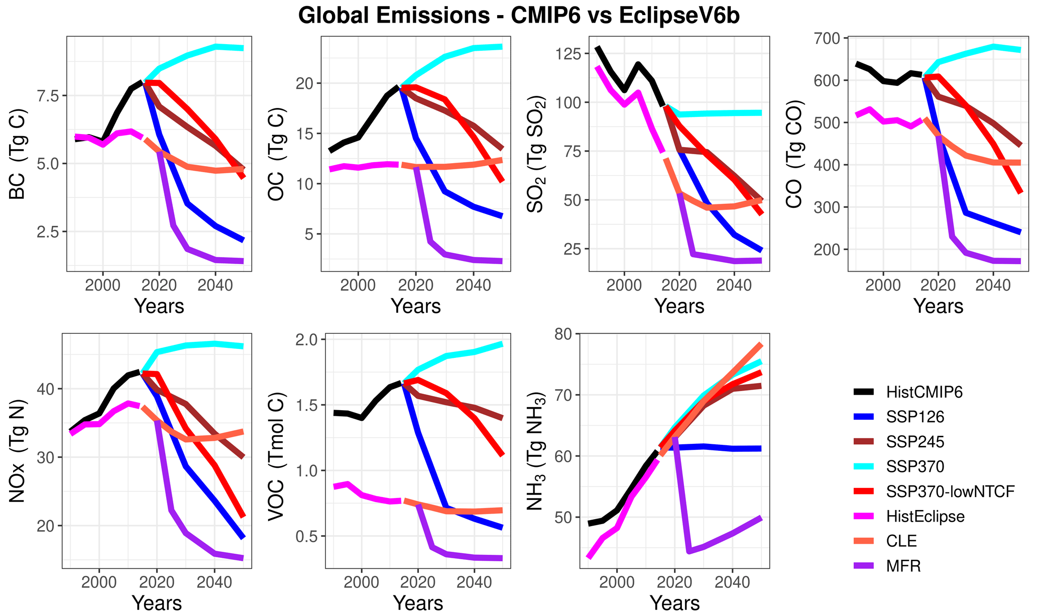
Figure 1Global recent past and future CMIP6 and Eclipse V6b anthropogenic emissions for different pollutants and scenarios.
2.3 Simulations
In order to contribute to the AMAP assessment report (AMAP, 2021), the GISS-E2.1 model participated with AMIP-type simulations, which aim to assess the trends of Arctic air pollution and climate change in the recent past, as well as with fully coupled climate simulations. Five fully coupled Earth system models (ESMs) simulated the future (2015–2050) changes in atmospheric composition and climate in the Arctic (>60∘ N), as well as over the globe. We have carried out two AMIP-type simulations, one with winds nudged to NCEP (standard AMIP-type simulation in AMAP) and one with freely varying winds, where both simulations used prescribed SSTs and sea ice (Table 1). The nudging extends from the first model layer up to 10 hPa, which is the top of the NCEP input. In the fully coupled simulations, we carried out two sets of simulations, each with three ensemble members, that used the CLE and MFR emission scenarios. Each simulation in these two sets of scenarios was initialized from a set of three fully coupled ensemble recent past simulations (1990–2014) to ensure a smooth continuation from CMIP6 to Eclipse emissions.
Table 1GISS-E2.1 simulations carried out in the Eclipse and CMIP6 ensembles.
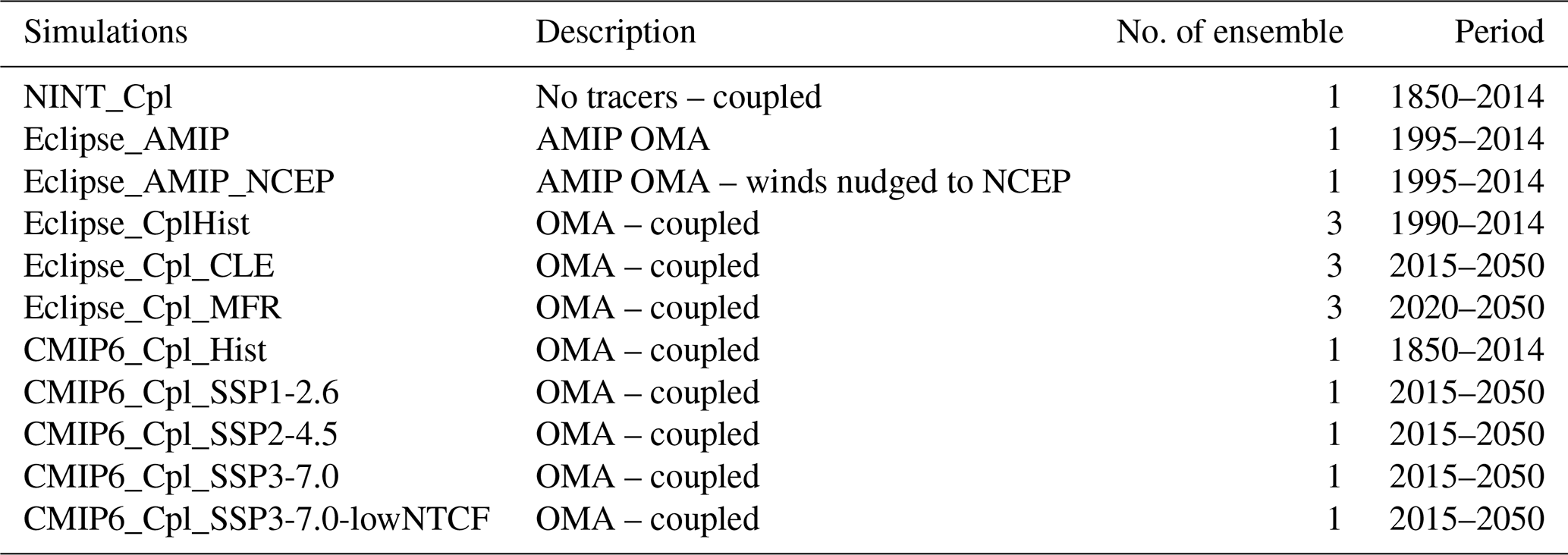
In addition to the AMAP simulations, we have also conducted CMIP6-type simulations in order to compare the climate aerosol burdens and their impacts on radiative forcing and climate impacts with those from the AMAP simulations. We have used the SSP1-2.6, 2-4.5, 3-7.0, and 3-7.0-lowNTCF scenarios representing different levels of emission mitigations in the CMIP6 simulations. SSP1 and SSP3 define various combinations of high or low socioeconomic challenges to climate change adaptation and mitigation, while SSP2 describes medium challenges of both kinds and is intended to represent a future in which development trends are not extreme in any of the dimensions but rather follow middle-of-the-road pathways (Rao et al., 2017). SSP1-2.6 scenario aims to achieve a 2100 radiative forcing level of 2.6 W m−2, keeping the temperature increase below 2 ∘C compared to the preindustrial levels. The SSP2-4.5 describes a middle-of-the-road socioeconomic family with a 4.5 W m−2 radiative forcing level by 2100. The SSP3-7.0 scenario is a medium–high reference scenario. SSP3-7.0-lowNTCF is a variant of the SSP3-7.0 scenario with reduced near-term climate forcer (NTCF) emissions. The SSP3-7.0 scenario has the highest methane and air pollution precursor emissions, while SSP3-7.0-lowNTCF investigates an alternative pathway for the Aerosols and Chemistry Model Intercomparison Project (AerChemMIP: Collins et al., 2017), exhibiting very low methane, aerosol, and tropospheric-ozone precursor emissions – approximately in line with SSP1-2.6. As seen in Table 1, we have conducted one transient fully coupled simulation from 1850 to 2014 and a number of future scenarios.
We have employed prescribed global and annual mean greenhouse (CO2 and CH4) concentrations, where a linear increase in global mean temperature of 0.2 ∘C per decade from 2019 to 2050 was assumed, which is approximately in line with the simulated warming rates for the SSP2-4.5 scenario (AMAP, 2021).
2.4 Observations
The GISS-E2.1 ensemble has been evaluated against surface observations of BC, organic aerosols (sum of OC and secondary organic aerosols (SOA), referred to as OA in the rest of the paper) and ; ground-based and satellite-derived AOD at 550 nm; and surface and satellite observations of surface air temperature, precipitation, sea surface temperature, sea-ice extent, cloud fraction, and liquid and ice water content in 1995–2014 period. The surface monitoring stations used to evaluate the simulated aerosol levels have been listed in Tables S1 and S2 in the Supplement.
2.4.1 Aerosols
Measurements of speciated particulate matter (PM), BC, , and (OA) come from three major networks: the Interagency Monitoring of Protected Visual Environments (IMPROVE) for Alaska (the IMPROVE measurements that are in the Arctic (>60∘ N) are all in Alaska), the European Monitoring and Evaluation Programme (EMEP) for Europe, and the Canadian Aerosol Baseline Measurement (CABM) for Canada (Tables S1 and S2). In addition to these monitoring networks, BC, OA, and measurements from individual Arctic stations were used in this study. The individual Arctic stations are Fairbanks and Utqiagvik, Alaska (part of IMPROVE, though their measurements were obtained from their PIs); Gruvebadet and Zeppelin mountain (Ny-Ålesund), Norway; Villum Research Station, Greenland; and Alert, Nunavut (with the latter being an observatory in the Global Atmosphere Watch Programme of the WMO and a part of CABM). The measurement techniques are briefly described in the Supplement.
AOD at 500 nm from the AErosol RObotic NETwork (AERONET, Holben et al., 1998) was interpolated to 550 nm AOD using the Ångström formula (Ångström, 1929). We also used a new merged AOD product developed by Sogacheva et al. (2020) using AOD from 10 different satellite-based products. According to Sogacheva et al. (2020), this merged product could provide a better representation of temporal and spatial distribution of AOD. However, it is important to note that the monthly aggregates of observations for both AERONET and the satellite products depend on availability of data and are not likely to be the true aggregate of observations for a whole month when only few data points exist during the course of a month. In addition, many polar-orbiting satellites take one observation during any given day and typically at the same local time. Nevertheless, these datasets are key observations currently available for evaluating model performances. Information about the uncertain nature of AOD observations can be found in previous studies (e.g., Sayer et al., 2018; Sayer and Knobelspiesse, 2019; Wei et al., 2019; Schutgens et al., 2020, Schutgens, 2020; Sogacheva et al., 2020).
2.4.2 Surface air temperature, precipitation, and sea ice
Surface air temperature and precipitation observations used in this study are from University of Delaware gridded monthly mean datasets (UDel; Willmott and Matsuura, 2001). UDel's 0.5∘ resolution gridded datasets are based on interpolations from station-based measurements obtained from various sources including the Global Historical Climate Network, the archive of Legates and Willmott, and others. The Met Office Hadley Centre's sea ice and sea surface temperature (HadISST; Rayner et al., 2003) was used for evaluating model simulations of sea ice and SSTs. HadISST data are an improved version of their predecessor known as global sea ice and sea surface temperature (GISST). HadISST data are constructed using information from a variety of data sources such as the Met Office marine database, International Comprehensive Ocean-Atmosphere Data Set, passive microwave remote sensing retrieval, and sea-ice charts.
2.4.3 Satellite observations used for cloud fraction and cloud liquid water and ice water
The Advanced Very High Resolution Radiometer (AVHRR-2) sensors aboard the NOAA and EUMETSAT polar-orbiting satellites have been flying since the early 1980s. These data have been instrumental in providing the scientific community with climate data records spanning nearly four decades. Tremendous progress has been made in recent decades in improving, training, and evaluating the cloud property retrievals from these AVHRR sensors. In this study, we use the retrievals of total cloud fraction from the second edition of EUMETSAT's Climate Monitoring Satellite Application Facility (CM SAF) Cloud, Albedo and surface Radiation dataset from AVHRR data (CLARA-A2, Karlsson et al., 2017a). This cloud property climate data record is available for the period 1982–2018. Its strengths and weaknesses, and inter-comparison with the other similar climate data records are documented in Karlsson and Devasthale (2018). Further dataset documentation including algorithm theoretical basis and validation reports can be found in Karlsson et al. (2017b).
Cloud liquid and ice water path estimates derived from the cloud profiling radar aboard CloudSat (Stephens et al., 2002) and constrained with another sensor aboard NASA's A-Train constellation, MODIS-Aqua (Platnick et al., 2015), are used for the model evaluation. These Level 2b retrievals, available through the 2B-CWC-RVOD product (Version 5), for the period 2007–2016 are analyzed. This constrained version is used instead of its radar-only counterpart, as it uses additional information about visible cloud optical depths from MODIS, leading to better estimates of cloud liquid water paths. Because of this constraint the data are available only for the daylit conditions and, hence, are missing over the polar regions during the respective winter seasons. The theoretical basis for these retrievals can be found at http://www.cloudsat.cira.colostate.edu/sites/default/files/products/files/2B-CWC-RVOD_PDICD.P1_R05.rev0_.pdf (last access: 26 October 2020). Being an active cloud radar, CloudSat provides orbital curtains with a swath width of just about 1.4 km. Therefore, the data are gridded at to avoid too many gaps or patchiness and to provide robust statistics.
3.1 Evaluation
The simulations are compared against surface measurements of BC, OA, , and AOD, as well as surface and satellite measurements of surface air temperature, precipitation, sea surface temperature, sea-ice extent, total cloud fraction, liquid water path, and ice water path described in Sect. 2.4, by calculating the correlation coefficient (r) and normalized mean bias (NMB). OA refers to the sum of primary organic carbon (OC) and secondary organic aerosol (SOA).
3.1.1 Aerosols
The recent past simulations are for BC, OA, SO4, and AOD (Table 2) against available surface measurements. The monthly observed and simulated time series for each station are accumulated per species in order to get full Arctic time series data, which also include spatial variation, to be used for the evaluation of the model. In addition to Table 2, the climatological mean (1995–2014) of the observed and simulated monthly surface concentrations of BC, OA, , and AOD at 550 nm (note that AOD is averaged over 2008, 2009, and 2014) is shown in Fig. 2. The AOD observation data for years 2008, 2009, and 2014 are used in order to keep the comparisons in line with the multi-model evaluations being carried out in the AMAP assessment report (AMAP, 2021). We also provide spatial distributions of the NMB, calculated as the mean of all simulations for BC, OA, SO4, and AOD in Fig. 3. The statistics for the individual stations are provided in Tables S3–S6 in the Supplement.
Table 2Annual mean normalized mean bias (NMB: %) and correlation coefficients (r) for the recent past simulations in the GISS-E2.1 model ensemble during 1995–2014 for BC, OA, , and 2008/09–2014 for AOD550 from AERONET and satellites.
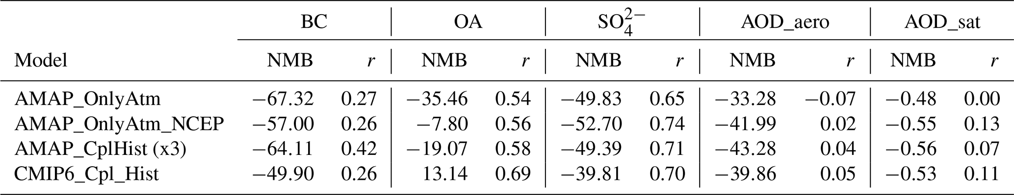
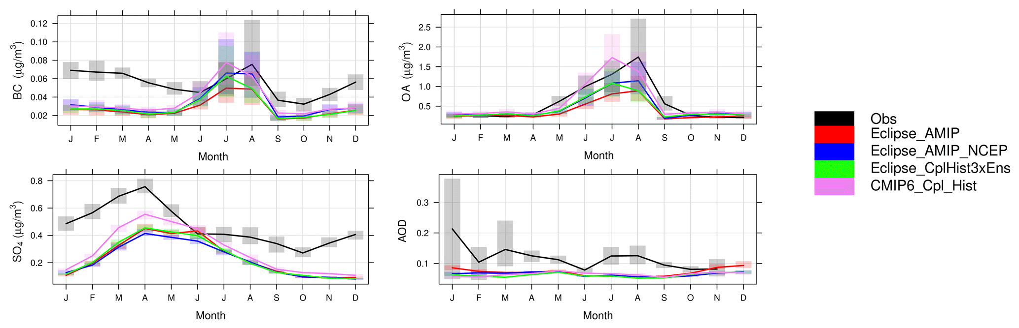
Figure 2Observed and simulated Arctic climatological (1995–2014) monthly BC, OA, , and AERONET AOD at 550 nm (2008/09–2014), along with the interannual variation shown in bars. The data present monthly accumulated time series for all stations that are merged together.
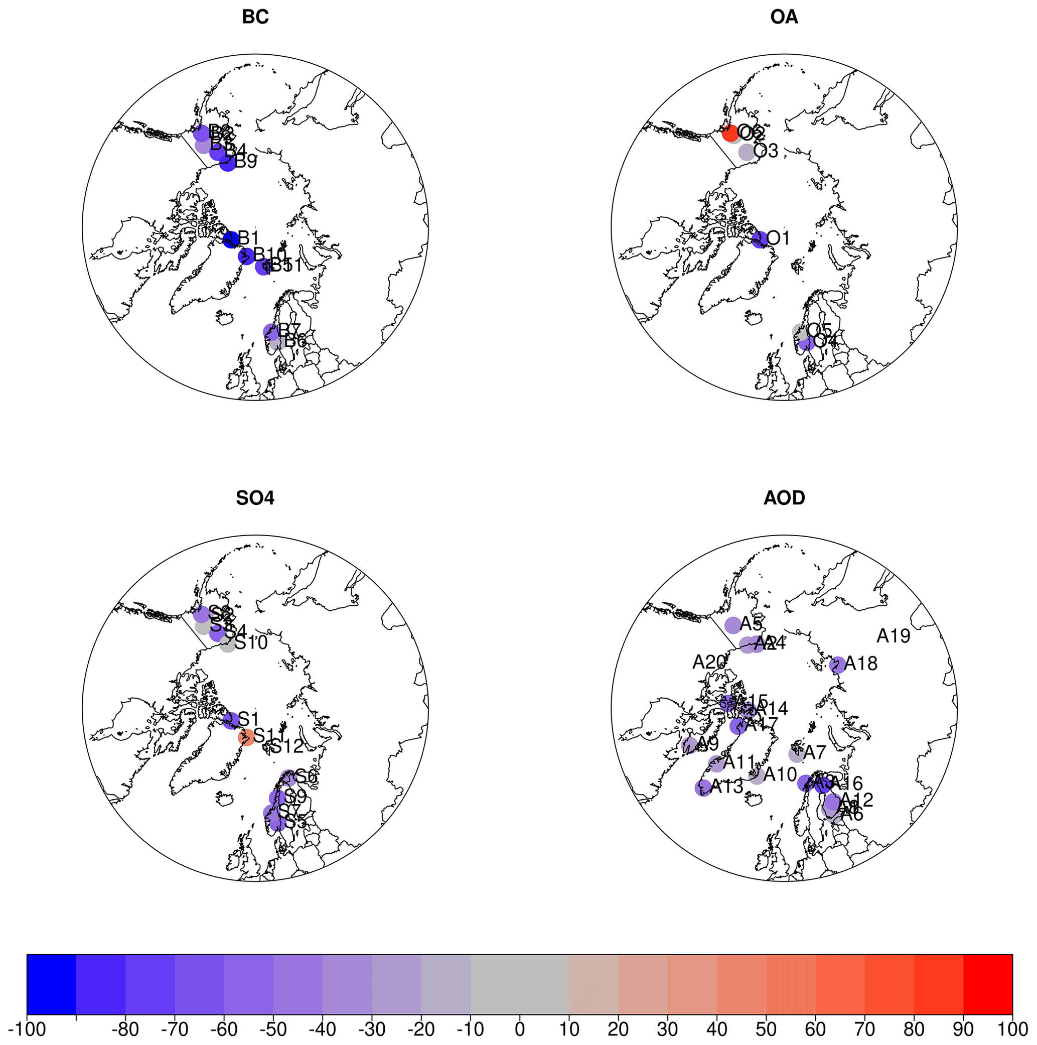
Figure 3Spatial distribution of normalized mean bias (NMB, in %) for climatological mean (1995–2014) BC, OA, , and AOD at monitoring stations, calculated as the mean of all recent past simulations.
Results showed overall an underestimation of aerosol species over the Arctic, as discussed below. Surface BC levels are underestimated at all Arctic stations from 15 % to 90 %. Surface OA levels are also underestimated from −5 % to −70 %, except for a slight overestimation of <1 % over Kårvatn (B5) and a large overestimation of 90 % over Trapper Creek (B6). Surface concentrations are also consistently underestimated from −10 % to −70 %, except for Villum Research Station (S11) over northeastern Greenland where there is an overestimation of 45 %. Finally, AODs are also underestimated over all stations from 20 % to 60 %. Such underestimations at high latitudes have also been reported by many previous studies (e.g., Skeie et al., 2011; Eckhardt et al., 2015; Lund et al., 2017, 2018; Schacht et al., 2019; Turnock et al., 2020), pointing to a variety of reasons including uncertainties in emission inventories, errors in the wet and dry deposition schemes, the absence or underrepresentation of new aerosol formation processes, and the coarse resolution of global models leading to errors in emissions and simulated meteorology, as well as in representation of point observations in coarse model grid cells. Turnock et al. (2020) evaluated the air pollutant concentrations in the CMIP6 models, including the GISS-E2.1 ESM, and found that observed surface PM2.5 concentrations are consistently underestimated in CMIP6 models by up to 10 µg m−3, particularly for the Northern Hemisphere winter months, with the largest model diversity near natural emission source regions and the polar regions.
The BC levels are largely underestimated in simulations by 50 % (CMIP6_Cpl_Hist) to 67 % (Eclipse_AMIP). The CMIP6 simulations have lower bias compared to Eclipse V6b simulations due to higher emissions in the CMIP6 emission inventory (Fig. 1). Within the Eclipse V6b simulations, the lowest bias (−57 %) is calculated for the Eclipse_AMIP_NCEP simulation, while the free climate and coupled simulations showed a larger underestimation (>62 %), which can be attributed to a better simulation of transport to the Arctic when nudged winds are used. The Eclipse simulations also show that the coupled simulations had slightly smaller biases ( %) compared to the AMIP-type free climate simulation (AMIP-OnlyAtm: %). The climatological monthly variation of the observed levels is poorly reproduced by the model with r values around 0.3. BC levels are mainly underestimated in winter and spring, which can be attributed to the underestimation of the anthropogenic emissions of BC, while the summer levels are well captured by the majority of the simulations (Fig. 2).
Surface OA concentrations are underestimated from 8 % (Eclipse_AMIP_NCEP) to 35 % (Eclipse_AMIP) by the Eclipse ensemble, while the CMIP6_Cpl_Hist simulation overestimated surface OA by 13 %. The Eclipse simulations suggest that the nudged winds lead to a better representation of transport to the Arctic, while the coupled simulations had smaller biases compared to the AMIP-type free climate simulation (AMIP-OnlyAtm), similar to BC. The climatological monthly variation of the observed concentrations are reasonably simulated, with r values between 0.51 and 0.69 (Table 2 and Fig. 2). As can be seen in Fig. S1, the OA levels are dominated by the biogenic SOA, in particular via α-pinene (monoterpenes) oxidation, compared to anthropogenic (by a factor of 4–9) and biomass burning (by a factor of 2–3) OA. While OC and BC are emitted almost from similar sources, this biogenic-dominated OA seasonality also explains why simulated BC seasonality is not as well captured, suggesting the underestimations in the anthropogenic emissions of these species, in particular during the winter. It should also be noted that GISS-E2.1 does not include marine VOC emissions except for DMS, while these missing VOCs such as isoprene and monoterpenes are suggested to be important sources for the summertime aerosol levels over the Arctic (Orellana et al., 2011; Karl et al., 2013; Schmale et al., 2021).
Surface levels are simulated with a smaller bias compared to the BC levels; however, they are still underestimated by 40 % (CMIP6_Cpl_Hist) to 53 % (Eclipse_AMIP_NCEP). The Eclipse_AMIP_NCEP simulation is biased higher ( %) compared to the Eclipse_AMIP ( %), probably due to higher cloud fraction simulated by the nudged version (see Sect. 3.1.6), leading to higher in-cloud production. The climatological monthly variation of observed concentrations is reasonably simulated in all simulations (r=0.65–0.74). The observed springtime maximum is well captured by the GISS-E2.1 ensemble, with underestimations in all seasons, mainly suggesting underestimations in anthropogenic SO2 emissions (Fig. 2), as well as simulated cloud fractions, which have high positive bias in winter and transition seasons, while in summer the cloud fraction is well captured with a slight underestimation. The clear-sky AOD over the AERONET stations in the Arctic region is underestimated by 33 % (Eclipse_AMIP) to 47 % (Eclipse_CplHist1). Similar negative biases are found with comparison to the satellite based AOD product (Table 2). The climatological monthly variation is poorly captured with r values between −0.07 and 0.07 compared to AERONET AOD and between 0 and 0.13 compared to satellite AOD. The simulations could not represent the climatological monthly variation of the observed AERONET AODs (Fig. 2).
3.1.2 Climate
The different simulations are evaluated against a set of climate variables, and the statistics are presented in Table 3a and b and in Figs. 4 and 5. The climatological mean (1995–2014) monthly Arctic surface air temperatures are slightly overestimated by up to 0.55 ∘C in the AMIP simulations, while the coupled ocean simulations underestimate the surface air temperatures by up to −0.17 ∘C. All simulations were able to reproduce the monthly climatological variation with r values of 0.99 and higher (Fig. 4). Results show that both absorbing (BC) and scattering aerosols (OC and ) are underestimated by the GISS-E2.1 model, implying that these biases can partly cancel out their impacts on radiative forcing due to aerosol–radiation interactions. This, together with the very low biases in surface temperatures, suggests that the effects of the anthropogenic aerosols on the Arctic climate via radiation are not the main driver in comparison to cloud indirect effects and forcing from greenhouse gases. The monthly mean precipitation has been underestimated by around 50 % by all simulations (Table 3a), with the largest biases during the summer and autumn (Fig. 4). The observed monthly climatological mean variation was very well simulated by all simulations, with r values between 0.80 and 0.90.
Table 3(a) Annual normalized mean biases (NMB: %) and correlation coefficients (r) for the recent past simulations in the GISS-E2.1 model ensemble in 1995–2014 for surface air temperature (Tsurf) and sea surface temperature (SST) in units of degree Celsius (∘C), precipitation (Precip), and sea-ice fraction (Sea ice). (b) Annual mean normalized mean biases (NMB: %) and correlation coefficients (r) for the recent past simulations in the GISS-E2.1 model ensemble in 1995–2014 for total cloud fraction (Cld Frac), liquid water path (LWP), and ice water path (IWP) in units of percent (%).
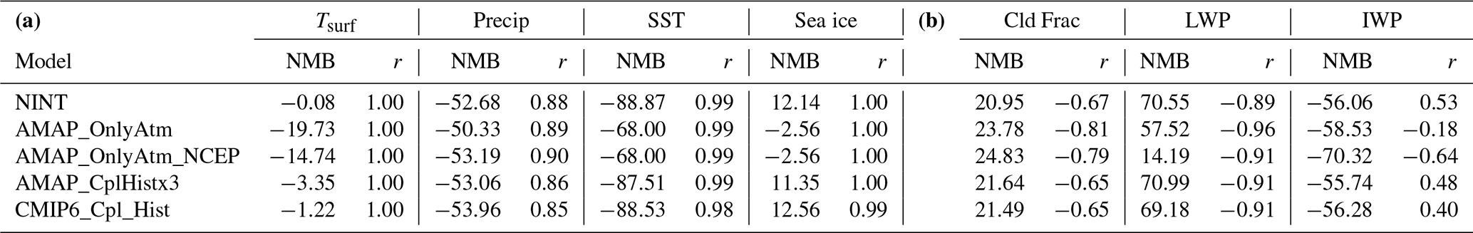

Figure 4Observed and simulated Arctic climatological (1995–2014) surface air temperature, precipitation, sea surface temperature, and sea ice, along with the interannual variation shown in bars. Obs denotes the UDel dataset for surface air temperature and precipitation, and HadISST denotes that for sea surface temperature and sea-ice extent. Note that the two AMIP runs (blue and red lines) for the SST and sea ice are on top of each other as they use that data to run as input.
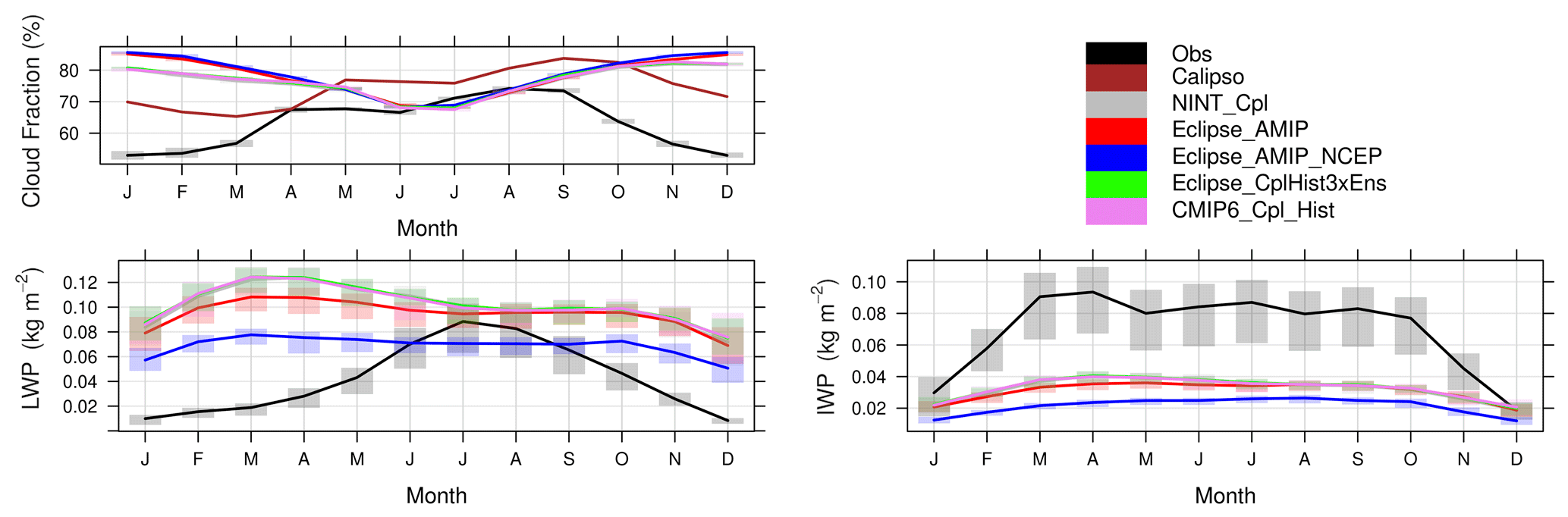
Figure 5Observed and simulated Arctic climatological total cloud fraction (1995–2014 mean), liquid water path (2007–2014 mean), and ice water path (2007–2014 mean), along with the interannual variation shown in bars. Obs denote CLARA-A2 for the cloud fractions and CloudSat for the LWP and IWP.
Arctic SSTs are underestimated by the ocean-coupled simulation up to −1.96 ∘C, while the atmosphere-only runs underestimated SSTs by −1.5 ∘C (Table 3a). The negative bias in atmosphere-only simulations is due to the different datasets used to drive the model, which is a combined product of HadISST and NOAA-OI2 (Reynolds et al., 2002), and to evaluate the model (Rayner et al., 2003), which is only HadISST. The monthly climatological mean variation is well captured with r values above 0.99 (Table 3a, Fig. 4), with a similar cold bias in almost all seasons. The sea-ice extent was overestimated by all coupled simulations by about 12 %, while the AMIP-type Eclipse simulations slightly underestimated the extent by 3 % (Table 3a). The observed variation was also very well captured with very high r values. The winter and spring biases were slightly higher compared to the summer and autumn biases (Fig. 4).
All simulations overestimate the climatological (1995–2014) mean total cloud fraction by 21 % to 25 % during the extended winter months (October through February), where the simulated seasonality is anti-correlated in comparison to AVHRR CLARA-A2 observations, whereas a good correlation is seen during the summer months irrespective of the observational data reference. The largest biases were simulated by the atmosphere-only simulations, with the nudged simulation having the largest bias (NMB=25 %). The coupled model simulations are closer to the observations during the recent past. On the other hand, the climatology of the annual-mean cloud fraction was best simulated by the nudged atmosphere-only simulation (Eclipse_AMIP_NCEP) with an r value of 0.40, while other simulations showed a poor performance ( to +0.10), except for the summer where the bias is lowest (Fig. 5). The evaluation against CALIPSO data however shows much smaller biases ( % to +6 %). This is because in comparison to the CALIPSO satellite that carries an active lidar instrument (CALIOP), the CLARA-A2 dataset has difficulties in separating cold and bright ice/snow surfaces from clouds, thereby underestimating the cloudiness during Arctic winters. Here both datasets are used for the evaluation as they provide different observational perspectives and cover the typical range of uncertainty expected from the satellite observations. Furthermore, while the CLARA-A2 covers the entire evaluation period in current climate scenario, CALIPSO observations are based on 10-year data covering the 2007–2016 period.
Figure 5 shows the evaluation of the simulations with respect to LWP and IWP. It has to be noted here that to obtain a better estimate of the cloud water content, the CloudSat observations were constrained with MODIS observations, which resulted in a lack of data during the months with darkness (October–March) over the Arctic (see Sect. 2.4.3). Hence, we present the results for the polar summer months only. As seen in Fig. 5, all simulations overestimated the climatological (2007–2014) mean polar summer LWP by up to almost 75 %. The smallest bias (14 %) is calculated for the nudged atmosphere only (Eclipse_OnlyAtm_NCEP), while the coupled simulations had biases of 70 % or more. Observations show a gradual increase in the LWP, peaking in July, whereas the model simulates a more constant amount for the nudged simulation and a slightly decreasing tendency for the other configurations. All model simulations overestimate LWP during the spring months. The atmosphere-only nudged simulations tend to better simulate the observed LWP during the summer months (June through September). The coupled simulations, irrespective of the emission dataset used, are closer to observations only during the months of July and August.
The climatological (2007–2014) mean polar summer IWP is slightly better simulated compared to the LWP, with biases within −60 % with the exception of the nudged Eclipse (Eclipse_AMIP_NCEP) simulation ( %). All simulations simulated the monthly variation well, with r values of 0.95 and more. In the Arctic, the net cloud forcing at the surface changes sign from positive to negative during the polar summer (Kay and L'Ecuyer, 2013). This change typically occurs in May driven mainly by shortwave cooling at the surface. Since the model simulates the magnitude of the LWP reasonably, particularly in summer, the negative cloud forcing can also be expected to be realistic in the model (e.g., Gryspeerdt et al., 2019). Furthermore, the aerosol and pollution transport into the Arctic typically occurs in the lowermost troposphere where liquid water clouds are prevalent during late spring and summer seasons (Stohl, 2006; Law et al., 2014; M. A. Thomas et al., 2019). The interaction of ice clouds with aerosols is, however, more complex, as ice clouds could have varying optical thicknesses, with mainly thin cirrus in the upper troposphere and relatively thicker clouds in the layers below. Without the knowledge on the vertical distribution of optical thickness, it is difficult to infer the potential impact of the underestimation of IWP on total cloud forcing and their implications.
3.2 Arctic burdens and radiative forcing due to aerosol–radiation interactions (RFARI)
The recent past and future Arctic column burdens for BC, OA, and for the different scenarios and emissions are provided in Fig. 6. In addition, Table 4 shows the calculated trends in the burdens for BC, OA, and for the different scenarios, while Table 5 provides the 1990–2010 and 2030–2050 mean burdens of the aerosol components. The BC and burdens started decreasing from the 1990s, while the OA burden remains relatively constant, although there is large year-to-year variability in all simulations. All figures show a decrease in burdens after 2015, except for the SSP3-7.0 scenario, where the burdens remain close to the 2015 levels. The high variability in BC and OA burdens over the 2000s is due to the biomass burning emissions from the Global Fire Emissions Database (GFED), which have not been harmonized with the no-satellite era. It should also be noted that these burdens can be underestimated considering the negative biases calculated for the surface concentrations and in particular for the AODs reported in Tables 2 and S2–S6.
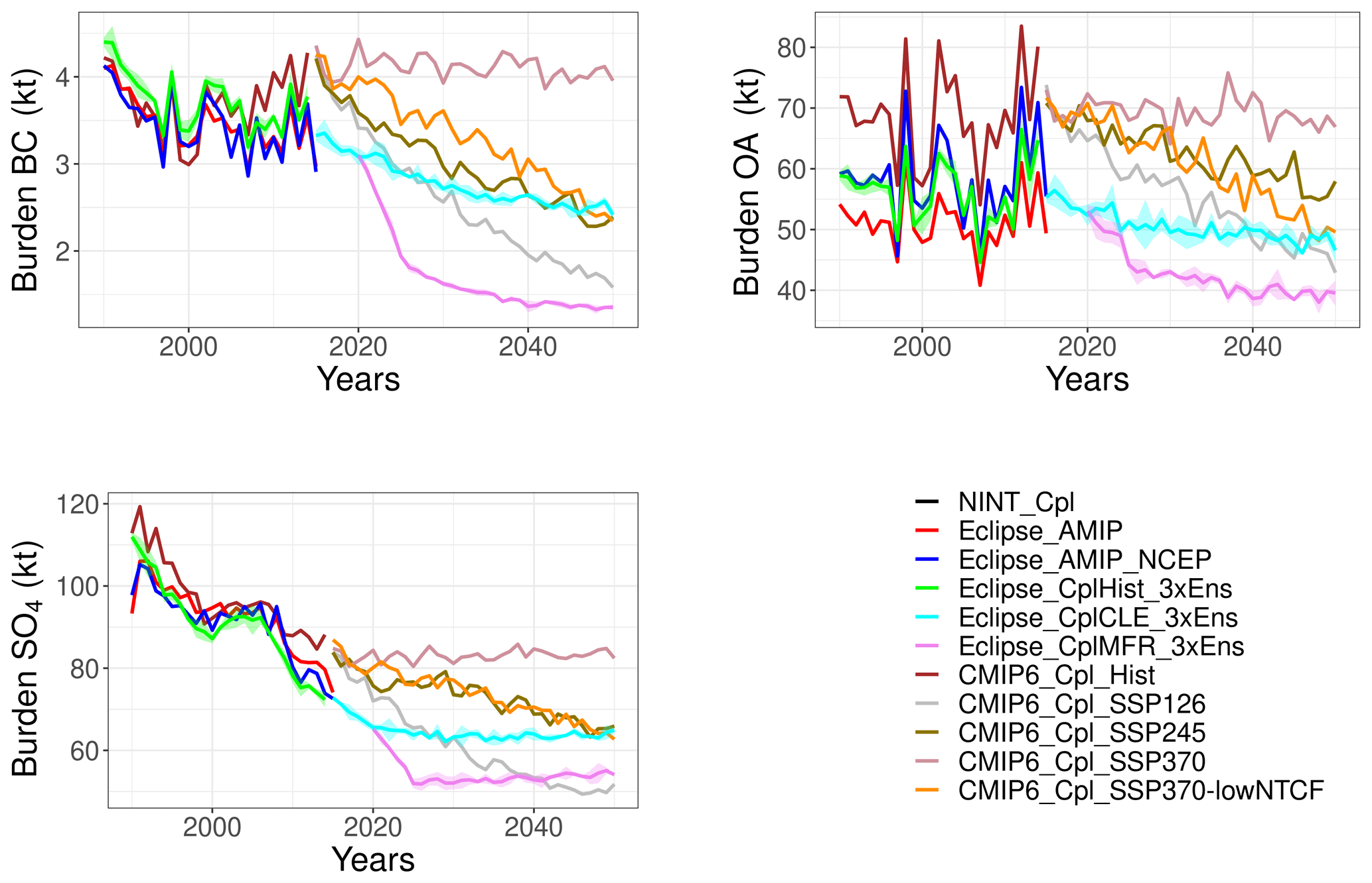
Table 4Trends in Arctic BC, OA, and burdens in the near past (1990–2014) and future (2030–2050) as calculated by the GISS-E2.1. The bold numbers indicate the trends that are statistically significant on a 95 % significance level.
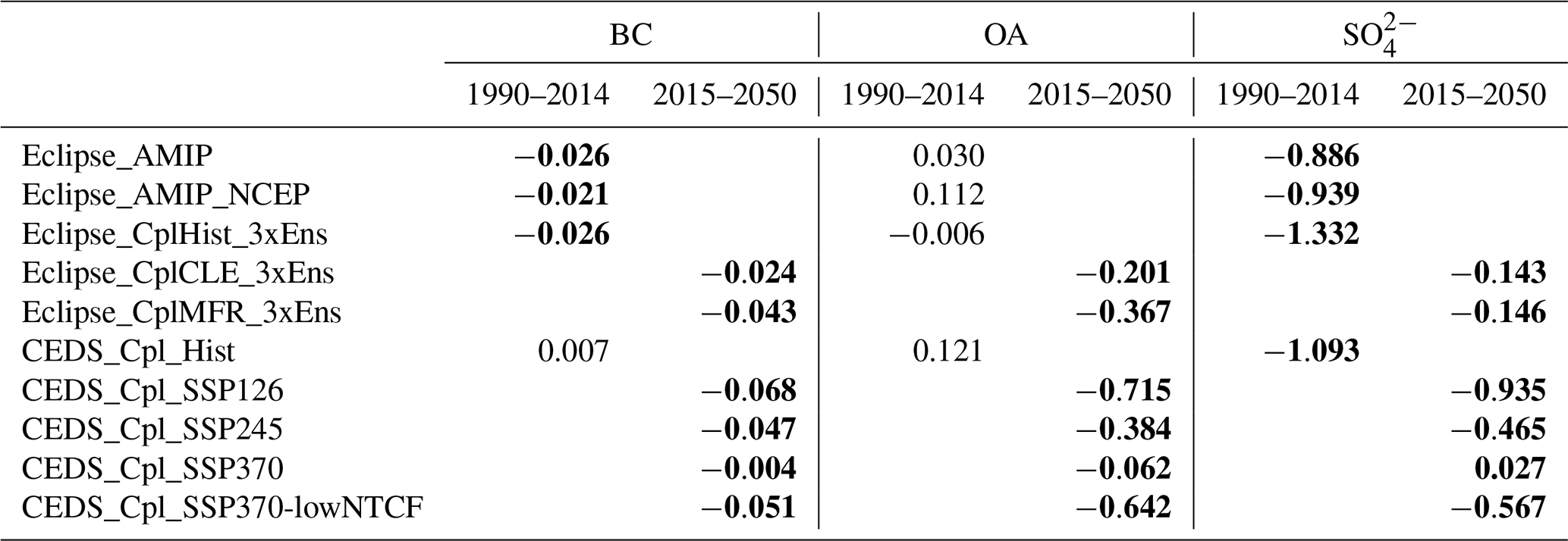
Table 5Arctic BC, OA, and burdens in 1990–2010 and 2030–2050 periods as calculated by the GISS-E2.1.

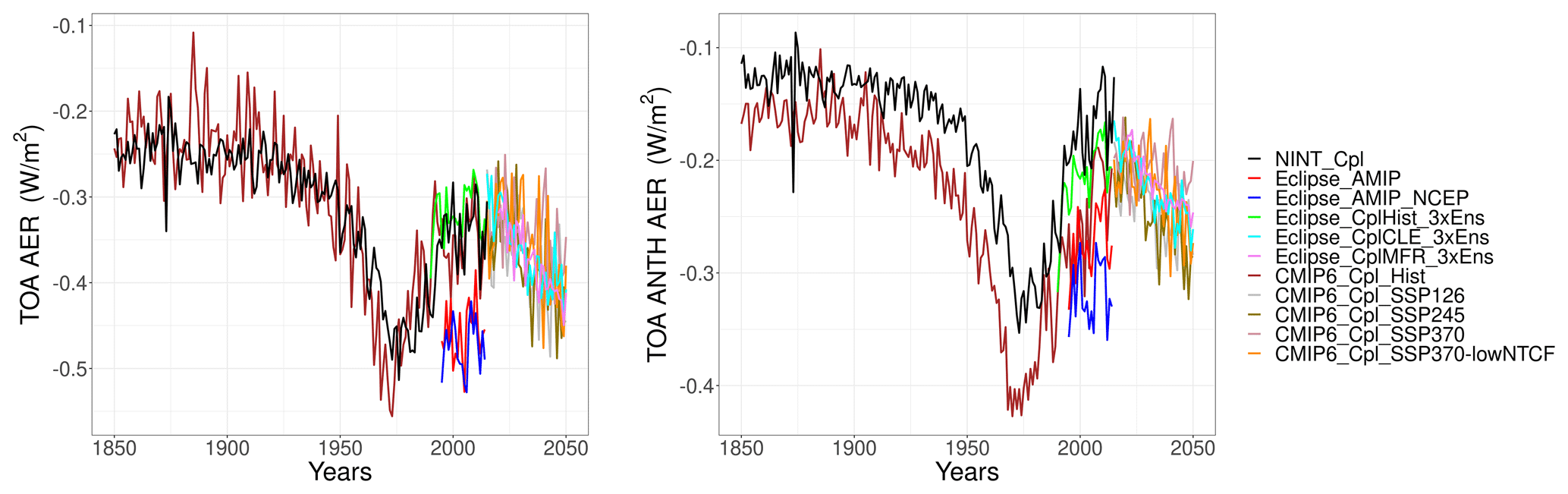
Figure 7Arctic RFARI from anthropogenic and natural aerosols () and only anthropogenic aerosols () in 1850–2050 as calculated by the full GISS-E2.1 ensemble.
In addition to the burdens of these aerosol species, the TOA radiative forcing due to aerosol–radiation interaction (RFARI) over the Arctic is simulated by the GISS-E2.1 ensemble. RFARI is calculated as the sum of shortwave and longwave forcing from the individual aerosol species between 1850 and 2050 is presented in Fig. 7. It is important to note that the present study uses the instantaneous forcing diagnostics from the model, which are calculated with a double call to the model's radiation code, with and without aerosols, as described in Bauer et al. (2020) and Miller et al. (2021), and not the effective radiative forcing. The transient cloud radiative effect in GISS-E.2.1 follows Ghan (2013), which calculates the difference in cloud radiative forcing with aerosol scattering and absorption omitted (Bauer et al., 2020). However, the present study only focuses on the RFARI. The model outputs separate forcing diagnostics for anthropogenic and biomass burning BC and OC, as well as biogenic SOA, making it possible to attribute the forcing to individual aerosol species. The negative RFARI has increased significantly since 1850 until the 1970s due to an increase in aerosol concentrations. Due to the efforts of mitigating air pollution and thus a decrease in emissions, the forcing became less negative after the 1970s until 2015. Figure 7 also shows a visible difference in the anthropogenic RFARI simulated by the NINT (prescribed aerosols) and OMA (interactive aerosols) simulations in the CMIP6 ensemble, where the anthropogenic RFARI by NINT simulation is less negative (by almost 30 %) compared to the OMA simulation (Fig. 7b). On the other hand, no such difference is seen in the net RFARI time series (Fig. 7a). This compensation is largely driven by the 50 % more positive dust and 10 % less negative sea-salt RFARI in the OMA simulation.
3.2.1 Black carbon
All simulations show a statistically significant (as calculated by Mann–Kendall trend analyses) decrease in the Arctic BC burdens (Table 4) between 1990–2014, except for the CMIP6_Cpl_Hist, which shows a slight non-significant increase that can be attributed to the large increase in global anthropogenic BC emissions in CMIP6 after year 2000 (Fig. 1). From 2015 onwards, all future simulations show a statistically significant decrease in the Arctic BC burden (Table 4). The Eclipse CLE ensemble shows a 1.1 kt (31 %) decrease in the 2030–2050 mean Arctic BC burden compared to the 1990–2010 mean, while the decrease in 2030–2050 mean Arctic BC burden is larger in the MFR ensemble (2.3 kt: 62 %). In the CMIP6 simulations, the 2030–2050 mean Arctic BC burdens decrease by 0.70 to 1.59 kt, being largest in SSP1-2.6 and lowest in SSP3-7.0-lowNTCF, while the SSP3-7.0 simulation leads to an increase of 0.43 kt (12 %) in 2030–2050 mean Arctic BC burdens. It is important to note that the change in burden simulated by the Eclipse CLE ensemble (−1.1 kt) is comparable with the change of −1 kt in the SSP2-4.5 scenario, consistent with the projected emission changes in the two scenarios (Fig. 1).
Table 6(a) RFARI for BC, OA, , and aerosols in 1990–2010 and 2030–2050 periods as calculated by the GISS-E2.1. (b) RFARI for total and anthropogenic aerosols in 1990–2010 and 2030–2050 periods as calculated by the GISS-E2.1.
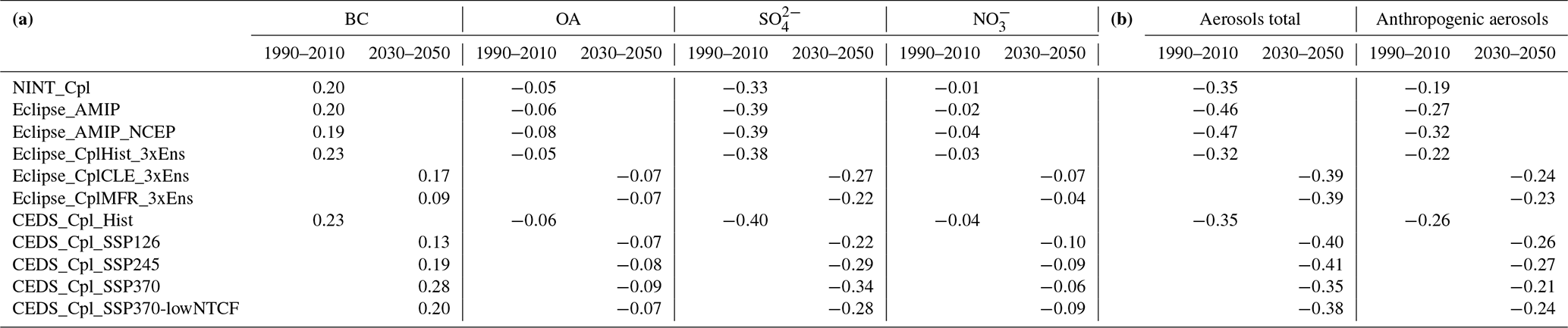
As seen in Table 6, the GISS-E2.1 ensemble calculated a BC RFARI of up to 0.23 W m−2 over the Arctic, with both CMIP6 and Eclipse coupled simulations estimating the highest forcing of 0.23 W m−2 for the 1990–2010 mean (Table 6a). This agrees with previous estimates of the BC RFARI over the Arctic (e.g., Schacht et al., 2019). In the future, the positive BC RFARI generally decreases (Fig. 6) due to lower BC emissions and therefore burdens, except for the SSP3-7.0 scenario, where the BC forcing becomes more positive by 0.05 W m−2 due to increasing BC emissions and burdens. The changes in the Arctic RFARI in Table 6a follow the Arctic burdens presented in Table 5 and emission projections presented in Fig. 1, leading to largest reductions in BC RFARI simulated in SSP1-2.6 (−0.10 W m−2). Similar to the burdens, the Eclipse CLE and CMIP6 SSP2-4.5 scenarios simulate a very close decrease in the 2030–2050 mean BC RFARI of −0.06 and −0.14 W m−2, respectively.
3.2.2 Organic aerosols
The Eclipse historical ensemble simulate a positive OA burden trend between 1990 and 2014; however, this trend is not significant at the 95 % confidence level (Table 4). The CMIP6_Cpl_Hist simulation gives a larger trend, due to a large increase in global anthropogenic OC emissions in CMIP6 (Fig. 1). The nudged AMIP Eclipse simulation calculates the largest 1990–2010 mean OA burden (57 kt), while the coupled simulation shows a slightly lower 1990–2010 mean burden (55 kt). This largest OA burden in the Eclipse_AMIP_NCEP simulation is attributed to the largest biogenic SOA burden calculated in this scenario, as well as a better-simulated transport from source regions due to the nudged winds (Fig. S1). The anthropogenic and biogenic contributions to SOA burdens in the coupled Eclipse and CMIP6 recent past simulations imply that the differences in the burdens between the two ensembles can be attributed to the different anthropogenic emissions datasets used in the Eclipse and CMIP6 simulations (Fig. S1), as well as the differences in SOA contributions due to simulated increases in the biogenic emissions (Fig. S5 in the Supplement). The AMIP-type Eclipse run simulates a lower 1990–2010 mean OA burden (50 kt), attributed to the smallest biogenic SOA burden in this scenario. The Eclipse CLE ensemble shows a decrease of 6.6 kt (12 %) in 2030–2050 mean OA burden compared to the 1990–2010 mean, while the MFR ensemble shows a larger decrease in the same period (15.2 kt: 27 %). The CMIP6 simulations show a much larger decrease in 2030–2050 mean Arctic OA burdens, with a decrease of 8.1 kt (SSP2-4.5) to 17 kt (SSP1-2.6), while the SSP3-7.0 simulation shows an increase in OA burdens in the same period by 1.3 kt (2 %). Similar to BC burdens, Eclipse CLE and CMIP6 SSP2-4.5 scenarios project similar changes in 2030–2050 mean OA burden (6.6 and 8.1 kt, respectively).
As shown in Table 6a, the Eclipse ensemble calculated an OA RFARI of −0.05 to −0.08 W m−2 for the 1990–2010 mean, where the nudged AMIP-type simulation shows the largest RFARI, due to the largest Arctic OA burden calculated for this period (Table 5). For the future, both Eclipse CLE and MFR ensembles show an increase in the negative 2030–2050 mean RFARI by −0.02 W m−2, which is very close to the increase in the negative forcing calculated for the various CMIP6 simulations (−0.01 to −0.03 W m−2). Following the burdens, the largest increase in the 2030–2050 mean OA RFARI is calculated for the SSP3-7.0 (−0.03 W m−2) and the lowest for SSP1-2.6 and 3-7.0-lowNTCF (−0.01 W m−2).
3.2.3 Sulfate
Regarding burdens, all simulations show a statistically significant negative trend both in 1990–2014 and in 2015–2050, as seen in Fig. 6 and Table 5. Both the nudged AMIP-type and coupled Eclipse simulations showed a 1990–2010 mean burden of 93 kt, while the AMIP-type simulation showed a slightly larger burden of 95 kt, attributed to the larger cloud fraction simulated in this model version (Table 2). For the 2015–2050 period, the Eclipse ensemble simulates a mean Arctic burden decrease of 30–40 kt (32 %–42 %), compared to the 1990–2010 mean, while CMIP6 ensemble simulates a reduction of 16–45 kt (16 %–45 %). The SSP2-4.5 and Eclipse CLE scenarios simulate a very similar decrease (30 kt) in 2030–2050 mean Arctic burdens, while the MFR and SSP1-2.6 scenarios also simulate comparable reductions in the burdens (Table 5). Following the emission projections, the SSP1-2.6 scenario gives the largest decrease (45 kt: 45 %), and the SSP3-7.0 scenario gives the smallest reduction (16 kt: 16 %) in Arctic 2030–2050 mean burdens.
The RFARI decreases (Fig. 6) following the decreasing emissions (Fig. 1) and burdens (Fig. 5). Both Eclipse and CMIP6 ensembles simulate a decrease in RFARI by 0.06–0.18 W m−2. The 2030–2050 mean RFARI follows the burdens (Table 6), with CLE and SSP2-4.5 giving similar decreases in the negative RFARI of 0.11 W m−2, while the Eclipse MFR and SSP1-2.6 simulates a very similar decrease in the 2030–2050 mean RFARI (0.16 and 0.18 W m−2, respectively).
3.2.4 Net aerosol radiative forcing
The coupled simulations in both the Eclipse and the CMIP6 ensemble show an Arctic RFARI of −0.32 to −0.35 W m−2 for the 1990–2010 mean, slightly lower than recent estimates (e.g., −0.4 W m−2 by Markowicz et al., 2021). In the Eclipse ensemble, W m−2 is calculated to be originated by the anthropogenic aerosols, while in the CMIP6 near-past simulations show a contribution of −0.19 to −0.26 W m−2 from anthropogenic aerosols (Table 6b). The AMIP-type Eclipse simulations calculated a much larger RFARI of −0.47 W m−2 for the same period, which can be mainly due to the increase in the positive forcing of the BC aerosols in the coupled simulations due to larger burdens. This effect is amplified due to the larger sea-ice concentration simulated with the coupled model, leading to brighter surfaces compared to the AMIP simulations. For the 2030–2050 period, the Eclipse ensemble simulated an increase in the negative RFARI by −0.07 W m−2, while the negative anthropogenic RFARI increased by only −0.02 W m−2, suggesting that the contribution from natural aerosols becomes more important in the future. The results show that the positive dust forcing is decreased by 0.03 W m−2 (from 0.12 to 0.09 W m−2 ), while the negative sea-salt forcing becomes more negative by −0.03 W m−2 due to the increase in ice-free ocean fraction due to melting of sea ice (see Sect. 3.3). For the same period, the CMIP6 future ensemble simulated an increase in the negative RFARI by −0.01 to −0.06 W m−2, with the largest change being in SSP1-2.6 and SSP2-4.5, mainly driven by the change in BC forcing (Table 6a). Table 6 also shows that the SSP1-1.6 simulates no change in the anthropogenic forcing, while SSP2-4.5 shows a similar increase of −0.01 W m−2 in the Eclipse ensemble. In contrast, the SSP3-7.0 and SSP3-7.0-lowNTCF simulates a large decrease in the anthropogenic negative RFARI by 0.05 and 0.02 W m−2, respectively.
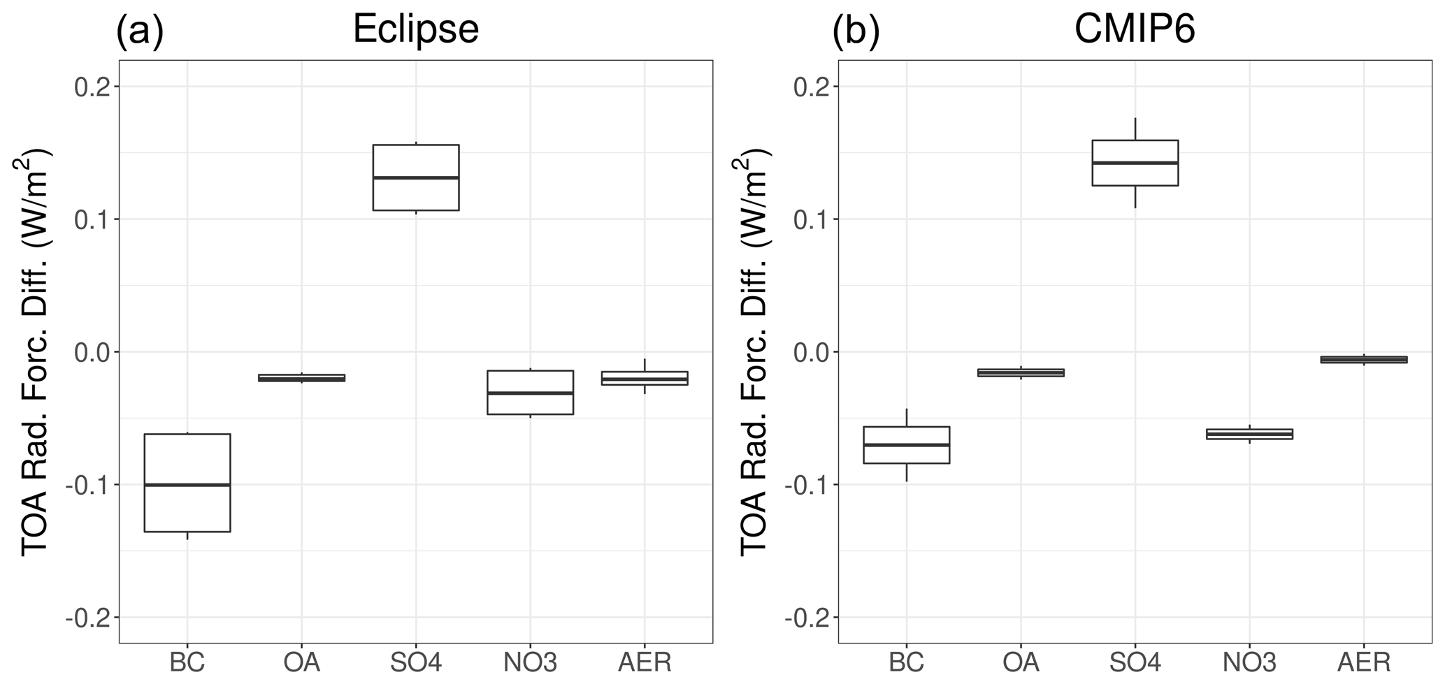
Figure 8Box–whisker plot showing the differences between 1990–2010 mean and 2030–2050 mean RFARI for the anthropogenic aerosol components (BC, OA, , and ) and their sum (AER) in the Eclipse ensemble (CLE and MFR: a) and the CMIP6 (SSP2-4.5 and SSP1-2.6: b) ensembles. The boxes show the median and the 25th and 75th percentiles. The upper whisker is located at the lower range of the maximum value and Q_3+1.5 IQR, whereas the lower whisker is located at the upper range of the smallest x value and Q_1−1.5 IQR, where IQR (interquartile range) is the box height (75th percentile−25th percentile).
The different behavior in the two ensembles is further investigated by looking at the aerosol–radiation forcing calculated for the individual aerosol species of BC, OA, , and presented in Fig. 8 that shows the box–whisker plots using the similar scenarios in the Eclipse (CLE and MFR) and CMIP6 (SSP2-4.5 and SSP1-2.6) ensembles. The increase in cooling effect of aerosols calculated by the Eclipse ensemble is attributed mainly to the decrease in BC as opposed to other aerosol species (Fig. 8). More negative forcing is calculated for the OA and , while the forcing is becoming less negative due to large reductions in SO2 emissions (Fig. 1). The net aerosol forcing is therefore slightly more negative. In the CMIP6 ensemble, the BC forcing does not change as much compared to the Eclipse ensemble to counteract the change in impact from , giving a more negative net aerosol forcing, which is slightly smaller compared to the Eclipse ensemble. The CMIP6 ensemble also simulates a larger increase in the negative forcing compared to the Eclipse ensemble (Shindell et al., 2013). Overall, the changes in the different aerosol species lead to a more negative aerosol forcing by mid-century (2030–2050) compared to the 1990–2010 period.

Figure 9Spatial distribution of the statistically significant annual mean Arctic RFARI (W m−2) changes between the 1990–2010 mean and the 2030–2050 mean as calculated by the GISS-E2.1 ensemble.
The spatial distributions of the statistically significant change in the Arctic RFARI in the 2030–2050 mean with respect to the 1990–2010 mean in the different ensemble members are presented in Fig. 9. Results show a decrease in the negative RFARI over Europe, and partly over North America, and an increase over the northern Pacific in all ensemble members. Globally, larger changes are simulated over East and South Asia (Fig. S2 in the Supplement), where largest anthropogenic emission reductions take place. The global net RFARI is dominated by the sea-salt particles, accounting for about 60 % of the 1990–2010 mean forcing of −2 to −2.3 W m−2 and the 2030–2050 mean forcing of −1.9 to 2.1 W m−2.
3.3 Climate change
3.3.1 Surface air and sea surface temperatures
The surface air temperature and sea-ice extent are calculated in the different simulations for the 1990–2050 period. As seen in Fig. 10, the Arctic surface air temperatures increase in all scenarios. Between 1990 and 2014, the surface air temperatures over the Arctic increased statistically significantly by 0.5 (Eclipse_CplHist) to 1 ∘C per decade (CMIP6_Cpl_Hist), with CMIP6 showing larger increases compared to the Eclipse ensemble (Table 7). On the other hand, the observed surface air temperature during 1990–2014 shows a smaller and statistically non-significant increase of 0.2 ∘C per decade. From 2015 onwards, surface air temperatures continue to increase significantly by 0.3 to 0.6 ∘C per decade, with larger increases in the Eclipse ensemble, due to larger reductions in the emissions and therefore in the burdens and associated RFARI.
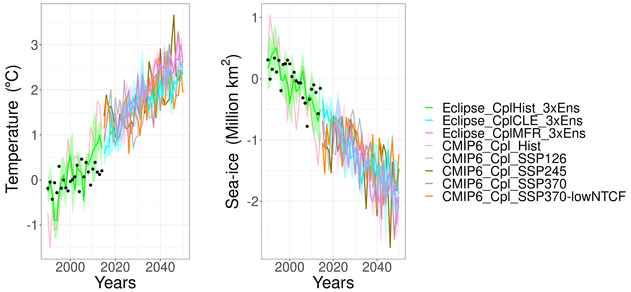
Figure 10Arctic annual mean surface air temperature and sea-ice extent anomalies in 2015–2050 based on the 1990–2010 mean as calculated by the GISS-E2.1 ensemble.
Table 7Trends in near-surface temperature (Tsurf) and annual mean sea-ice extent in 1990–2010 and 2030–2050 periods as calculated by the GISS-E2.1. The bold numbers indicate the changes in the 2030–2050 mean compared to the 1990–2010 mean that are statistically significant on a 95 % significance level.
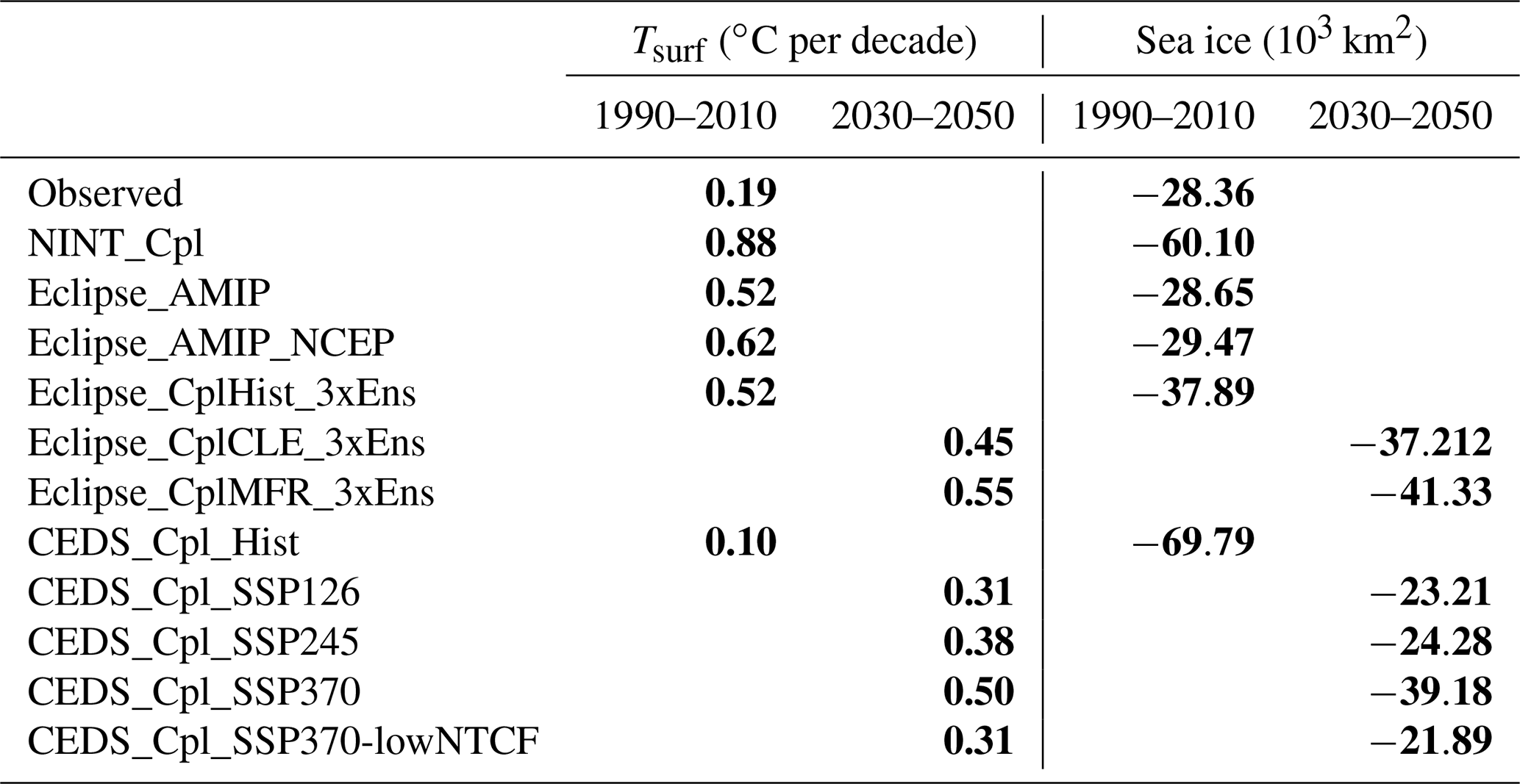
Table 8Near-surface temperature (Tsurf) and September mean sea-ice extent in 1990–2010 and 2030–2050 periods as calculated by the GISS-E2.1. The bold numbers indicate the changes in the 2030–2050 mean compared to the 1990–2010 mean that are statistically significant on a 95 % significance level.
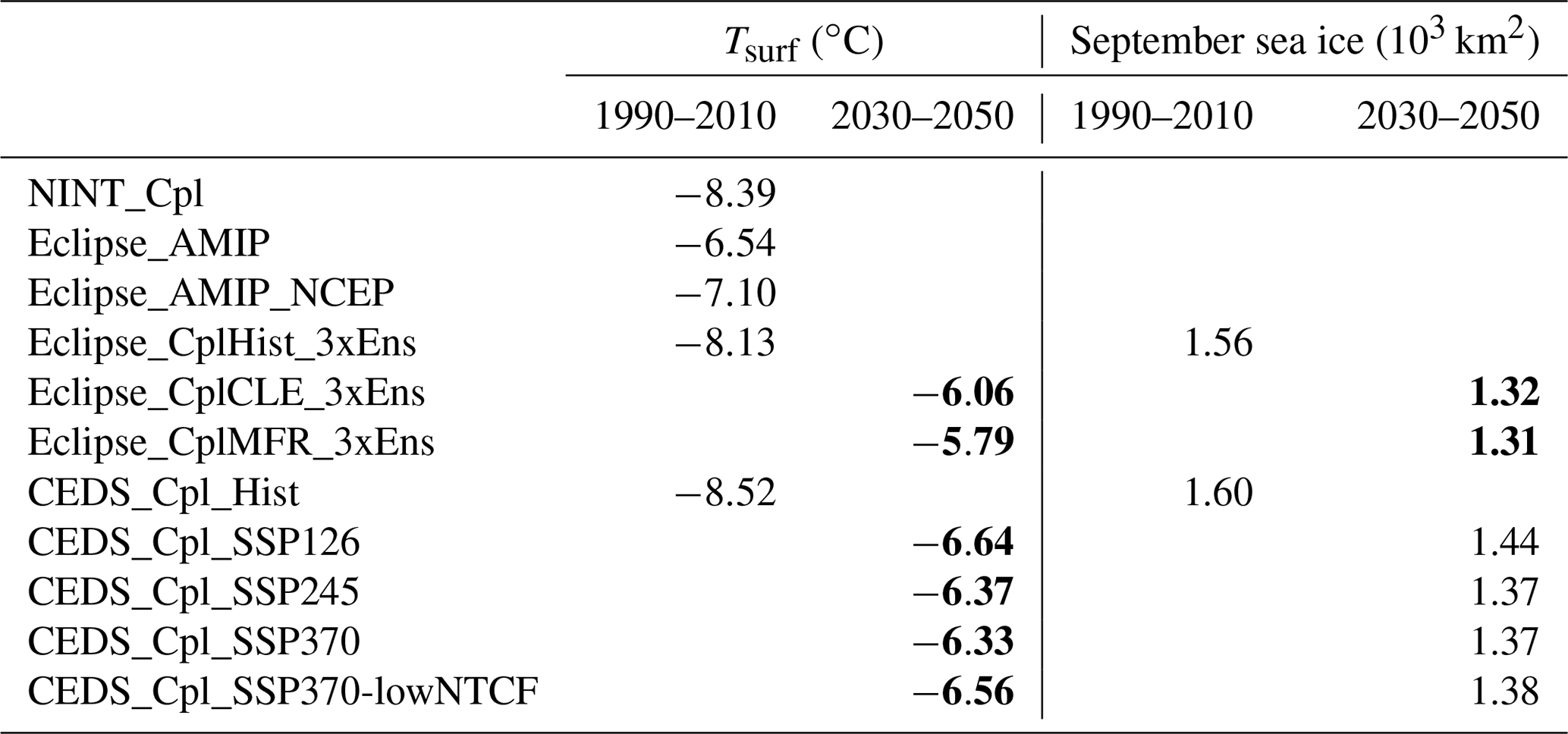
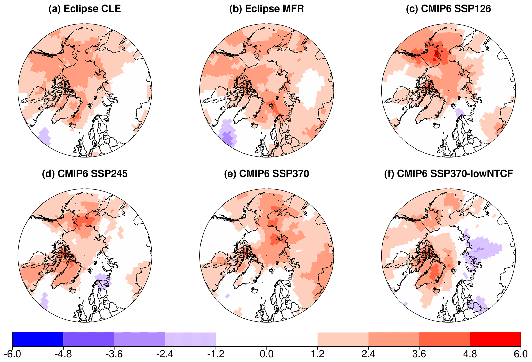
Figure 11Spatial distribution of the statistically significant annual mean Arctic surface air temperature (∘C) changes between the 1990–2010 mean and the 2030–2050 mean as calculated by the GISS-E2.1 ensemble.
The 2030–2050 mean surface air temperatures are projected to increase by 2.1 and 2.3 ∘C compared to the 1990–2010 mean temperature (Table 8, Fig. 10) according to the Eclipse CLE and MFR ensembles, respectively, while the CMIP6 simulation calculated an increase of 1.9 (SSP1-2.6) to 2.2 ∘C (SSP3-7.0). Changes in both ensembles are statistically significant on a 95 % level. These warmings are smaller compared to the 4.5–5 ∘C warmer 2040 temperatures and compared to the 1950–1980 average in the CMIP6 SSP1-2.6, SSP2-4.5, and SSP3-7.0 scenarios reported by Davy and Outten (2020). It should however be noted that due to the different baselines used in the present study (1990–2010) and the 1950–1980 baseline used in Davy and Outten (2020), it is not possible to directly compare these datasets. Figure 11 shows the spatial distributions of the statistically significant (as calculated by Student t test) Arctic surface air temperature change between the 1990–2010 mean and the 2030–2050 mean for the individual Eclipse and CMIP6 future scenarios. All scenarios calculate a warming in the surface air temperatures over the central Arctic, while there are differences over the land areas. The Eclipse CLE and MFR ensembles show similar warming mainly over the Arctic ocean as well as North America and Northeast Asia and cooling over the Greenland Sea. The latter is a well-known feature of observations and future projections, linked to the deep mixed layer in the area, and declines in the Atlantic meridional circulation (e.g., IPCC, 2014; Menary and Wood, 2018; Keil et al., 2020). There are also differences between the Eclipse and the CMIP6 ensembles as seen in Fig. 11. All CMIP6 scenarios show a warming over the central Arctic and a limited cooling over northern Scandinavia, following the changes in RFARI shown in Fig. 9, except for the SSP3-7.0 scenario that shows no cooling in the region. The SSP3-7.0-lowNTCF scenario shows an additional cooling over Siberia. These warmings are comparable with earlier studies, such as Samset et al. (2018) estimating a warming of 2.8 ∘C, attributed to aerosols.
3.3.2 Sea ice
The Arctic sea-ice extent is found to decrease significantly in all simulations (Fig. 10 and Table 7). Similar to the near-surface temperatures, during the 1990–2014 period, the CMIP6 ensemble simulated a large decrease in sea-ice extent compared to the Eclipse ensemble. On the other hand, the CMIP6_Cpl_Hist largely overestimated the observed decrease of 30 000 km2 yr−1. This overestimation has also been reported for some of the CMIP5 and CMIP6 models (Davy and Outten, 2020). After 2015, the Eclipse CLE ensemble projected larger decreases in the sea-ice extent compared to the CMIP6 ensemble (Table 7), in agreement with the changes in the near-surface temperatures. The evolutions of March and September sea-ice extents, representing the Arctic annual maximum and minimum extents, respectively, are also analyzed. The Eclipse ensemble projects a decrease of 23 000±11 000 km2 yr−1 in March sea-ice extent during the 2015–2050 period, while the CMIP6 ensemble projects a decrease of 10 000±6000 km2 yr−1 for the same period, both statistically significant. In September, much larger decreases are projected by both ensembles. The Eclipse ensemble simulates a decrease of 64 000±10 000 km2 yr−1 in the 2015–2050 period, while the CMIP6 ensemble predicts a decrease of 50 000±20 000 km2 yr−1.
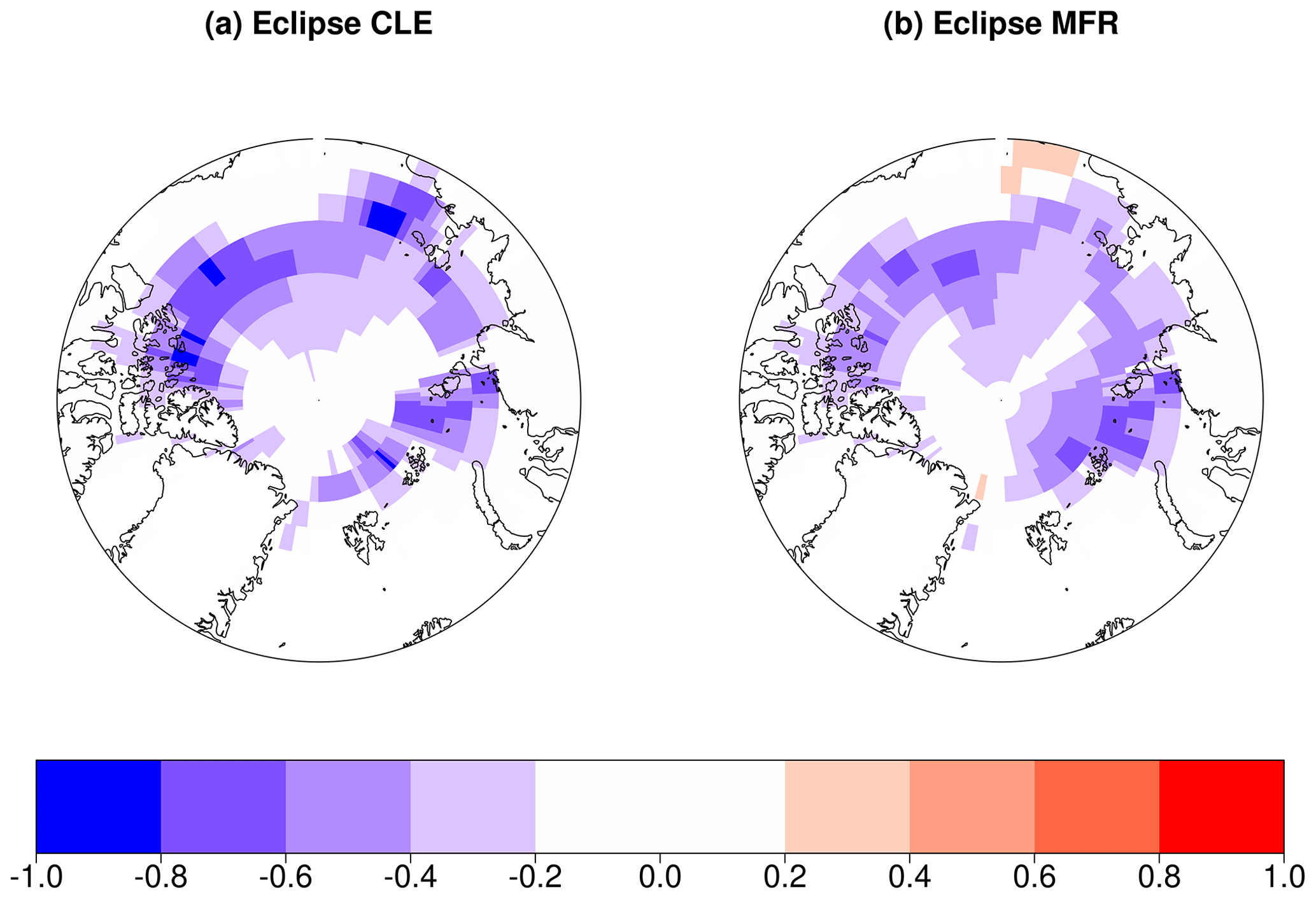
Figure 12Spatial distribution of the statistically significant September Arctic sea-ice fraction change between the 1990–2010 mean and the 2030–2050 mean as calculated by the GISS-E2.1 Eclipse ensemble (CMIP6 ensemble is not shown due to statistically insignificant changes calculated by the Student t test).
The 2030–2050 annual mean sea-ice extent (Table 8) is projected to be 1.5 and 1.7 million square kilometers lower compared to the 1990–2010 mean in the Eclipse CLE and MFR scenarios, respectively, both statistically significant on a 95 % level. The CMIP6 simulations predict a lower decrease in sea-ice extent by 1.2–1.5 million square kilometers; however, these changes are not statistically significant. These results are comparable with the results from the CMIP6 models (Davy and Outten, 2020). In the 2030–2050 March mean the sea-ice extent is projected to be 925 000 km2 lower in the Eclipse ensemble (statistically significant), while the CMIP6 ensemble projects a decrease of 991 000 km2 (not statistically significant). A much larger decrease is projected for the 2030–2050 September mean: 2.6 million and 2.3 million square kilometers in Eclipse and CMIP6 ensembles, respectively. As seen in Fig. 12, the Eclipse ensemble predicts an up to 90 % lower September sea-ice fraction in a band marking the maximum retreat of the sea-ice line at the end of the summer, while the changes simulated by the CMIP6 ensemble are not statistically significant on a 95 % level (therefore not shown in Fig. 11), which can be attributed to the single ensemble member per scenario in the CMIP6 ensemble, as well as the not-significant changes in the near-surface temperatures (not shown). In March (Fig. S3 in the Supplement), the Eclipse ensemble simulated a decrease in maximum sea-ice extent at the end of winter over the northern Pacific, while the CMIP6 ensemble did not show any statistically significant changes in sea ice. In addition, the Eclipse ensemble shows a decrease over the north Atlantic close to Greenland. All simulations show a similar and statistically significant decrease in annual mean sea-ice extent (Fig. S4 in the Supplement) over the central Arctic, with the CMIP6 ensemble showing also some increase in the sea-ice extent over the Canadian Arctic, which is largest in SSP3-7.0.
The retreat in sea-ice extent also led to an increase in oceanic emissions of DMS and sea salt (Fig. S5); however, the increases are not significant on a 95 % significance level. The simulated increase, in particular for the DMS emissions, is slightly larger in the Eclipse ensemble compared to the CMIP6 ensemble, due to a larger decrease in sea-ice extent in the Eclipse ensemble. Also note that GISS-E2.1 is using prescribed and fixed maps of DMS concentration in the ocean. When ocean locations that are year-round under sea ice at present get exposed, the DMS that would exist in that seawater is not included in the simulations, likely underestimating the increased flux of DMS into the atmosphere as the sea-ice retreats.
The GISS-E2.1 earth system model has been used to simulate the recent past (1990–2014) and future (2015–2050) aerosol burdens and their climate impacts over the Arctic. An ensemble of 17 simulations has been conducted using historical and future anthropogenic emissions and projections from CMIP6 and Eclipse V6b, with the latter supporting the ongoing Arctic Monitoring and Assessment Programme.
The evaluation of the recent past simulations shows underestimates of Arctic surface aerosol levels by up to 50 %, with the smallest biases calculated for the simulations where winds are nudged and sea surface temperature and sea ice are prescribed (AMIP-type: atmosphere-only). An exception is , where the nudged Eclipse AMIP simulation had the highest bias, due to the high cloud bias that leads to more in-cloud sulfate production from SO2. The model skill analyses indicate slightly better performance of the CMIP6 version of the GISS-E2.1 model in simulating both the aerosol levels and climate parameters compared to the Eclipse version. In addition, the underestimations in summertime cloud fraction suggests missing sources of aerosols, in particular the local marine sources. GISS-E2.1 does not include marine VOC emissions except for DMS, which are suggested to be important for the summertime cloud properties over the Arctic (Ornella et al., 2011; Karl et al., 2013; Schmale et al., 2021). Results also suggest that the underestimation of both absorbing and scattering aerosol levels can partly cancel out their impacts on RFARI and near-surface temperatures as the temperatures are very well reproduced by the model.
From 2015 onwards, all simulations, except for the worst-case CMIP6 scenario SSP3-7.0, show a statistically significant decrease in the Arctic BC, OA, and burdens, with the CMIP6 ensemble simulating larger aerosol burdens than Eclipse, while the Eclipse ensemble shows larger reductions (10 %–60 %) in Arctic aerosol burdens compared to the reduction simulated by the CMIP6 ensemble (10 %–45 %). The largest burden reductions are calculated by the highly ambitious emission reductions in the two ensembles; i.e., the Eclipse MFR (25 %–60 %) and the CMIP6 SSP1-2.6 (25 %–45 %).
The present-day (1990–2010 mean) CMIP6 and Eclipse simulations calculated an aerosol radiative forcing due to aerosol–radiation interactions (RFARI ) of −0.32 to −0.35 W m−2. For the same period, the atmosphere-only (AMIP) Eclipse simulations calculated a much larger negative RFARI of −0.47 W m−2. This smaller RFARI by the coupled simulations is mainly due to larger BC burdens in the coupled simulations, leading to more positive forcing, which is amplified by the larger albedo effect due to larger sea-ice extent simulated in the coupled simulations. In the 2030–2050 period, the Eclipse ensemble simulated a RFARI of W m−2, of which W m−2 is attributed to the anthropogenic aerosols (BC, OA, , and ). For the same period, the worst-case CMIP6 scenario (SSP3-7.0) simulated a similar RFARI (−0.35 W m−2) compared to the 1990–2010 mean, while large emission reductions led to a more negative RFARI (−0.40 W m−2), mainly due to decrease in the positive forcing of the BC aerosols. Overall, the Eclipse ensemble simulated slightly larger changes in the RFARI over the 2015–2050 period, relative to the 1990–2010 mean, compared to the CMIP6 ensemble, which can be attributed to the larger reductions in burdens in the Eclipse ensemble. The differences between the two ensembles are further attributed to differences in the BC and forcings. The results suggest that the different anthropogenic emission projections lead to only small differences in how the RFARI will evolve in the future over the Arctic.
The future scenarios with the largest aerosol reductions, i.e., MFR in the Eclipse and SSP1-2.6 in the CMIP6 ensemble, project the largest warming and sea-ice retreat. The Eclipse ensemble shows a slightly larger warming of 2030–2050 mean surface air temperatures compared to the 1990–2010 mean warming (2.1 to 2.5 ∘C) compared to that from the CMIP6 ensemble (1.9 to 2.2 ∘C). Larger warming in the Eclipse ensemble also resulted in a slightly larger reduction in sea-ice extent (−1.5 to −1.7 million square kilometers in CLE and MFR, respectively) in the 2030–2050 mean compared to the reduction in the CMIP6 scenario (−1.3 to −1.6 million square kilometers in SSP1.2-6 and SSP3-7.0, respectively). However, the changes simulated by the two ensembles are within 1 standard deviation of each other.
The overall results showed that the aerosol burdens will substantially decrease in the short- to mid-term future, implying improvements in impacts on human health and ecosystems. However, the impacts of aerosols on the radiative forcing can be amplified by the sea-ice extent. Results also show that even the scenarios with largest emission reductions, i.e., Eclipse MFR and CMIP6 SSP1-2.6, lead to similar impact on the future Arctic surface air temperatures and sea-ice loss compared to scenarios with very little mitigation such as the CMIP6 SSP3-7.0, exacerbating the dominant role played by well-mixed greenhouse gases and underlining the importance of continued greenhouse gas reductions.
The GISS-E2.1 model can be downloaded freely from the following website: https://simplex.giss.nasa.gov/snapshots/ (Aleinov, 2021).
HadISST data were obtained from https://www.metoffice.gov.uk/hadobs/hadisst/ (Met Office Hadley Centre, 2021) and have a © British Crown Copyright, Met Office, provided under a Non-Commercial Government Licence (http://www.nationalarchives.gov.uk/doc/non-commercial-government-licence/version/2/; last access: 3 July 2021). UDel_AirT_Precip data were provided by the NOAA/OAR/ESRL PSL, Boulder, Colorado, USA, from their website at https://psl.noaa.gov/ (Willmott and Matsuura, 2021). Alert sulfate data were provided by Sangeeta Sharma, and elemental carbon (EC) and OA data were provided by Lin Huang as part of Canadian Aerosol Baseline Measurement (CABM) program at ECCC. We would like to thank operators and technicians for the collection of filters, calibration, and analysis, as well as the Canadian Forces Services Alert for the operation of the military base. These datasets are also available on the Global Atmospheric Watch Programme, World Data Center for Aerosols, EBAS database (http://ebas.nilu.no/default.aspx, Norwegian Institute for Air Research, 2021). Aside from Alert, Canada’s surface air quality data are from the National Atmospheric Pollution Surveillance network (NAPS: https://open.canada.ca/data/en/dataset/1b36a356-defd-4813-acea-47bc3abd859b, Analysis and Air Quality Section Environment Canada, 2021).
Fairbanks aerosol measurements are from William Simpson and KC Nattinger. Aside from Fairbanks, Alaska measurements are from the IMPROVE network. IMPROVE is a collaborative association of state, tribal, and federal agencies, as well as international partners. The US Environmental Protection Agency is the primary funding source, with contracting and research support from the National Park Service. The Air Quality Group at the University of California, Davis, is the central analytical laboratory, with ion analysis provided by the Research Triangle Institute and carbon analysis provided by the Desert Research Institute. European measurements are from the EMEP network and obtained from the EBAS database (http://ebas.nilu.no, last access: 3 July 2021). Other European data include the Gruvebadet measurements, for which we acknowledge Mauro Mazzola (mauro.mazzola@cnr.it), Stefania Gilardoni (stefania.gilardoni@cnr.it), and Angelo Lupi (angelo.lupi@cnr.it) from the Institute of Polar Sciences for Gruvabadet eBC measurements, as well as Rita Traversi (rita.traversi@unifi.it), Mirko Severi (mirko.severi@unifi.it), and Silvia Becagli (silvia.becagli@unifi.it) from the University of Florence (http://www.isac.cnr.it/~radiclim/CCTower/?Data:Aerosol, National Research Council of Italy, 2021); the Zeppelin datasets, for which we acknowledge Vito Vitale and Angelo Lupi (also available on http://ebas.nilu.no); and the Villum Research Station datasets (http://www.villumresearchstation.dk, Aarhus University, 2021) from Henrik Skov (hsk@envs.au.dk; also available at http://ebas.nilo.no). The AERONET AOD measurements were obtained from NASA's Goddard Space Flight Center (https://aeronet.gsfc.nasa.gov/new_web/index.html, NASA, 2021). The authors acknowledge Larisa Sogacheva and the AEROSAT team for satellite-based merged AOD data.
The supplement related to this article is available online at: https://doi.org/10.5194/acp-21-10413-2021-supplement.
UI coordinated the study; conducted the model simulations, model evaluation, and analyses of the simulations; and wrote the manuscript. KT and GF supported the model simulations and processing of the Eclipse V6b emissions for the GISS-E2.1 model. JPF contributed to the plotting of the spatial distributions by further developing the autoimage R package (French, 2017). RM prepared and provided the AOD measurements, as well as the surface air temperature, sea surface temperature, and sea-ice data. MAT prepared the cloud observation data. CHW prepared the Arctic surface aerosol measurement data. KvS coordinated the experimental setup for the Eclipse simulations in the framework of the ongoing AMAP assessment. ZG prepared and provided the Eclipse V6b anthropogenic emissions. HS and DCT prepared the Villum Research Station aerosol data. JB and PL contributed to analyses of aerosols and climate parameters, respectively, and manuscript writing. All authors contributed to the analyses and interpretation of the results, as well as to the writing of the manuscript.
The authors declare that they have no conflict of interest.
Publisher's note: Copernicus Publications remains neutral with regard to jurisdictional claims in published maps and institutional affiliations.
This article is part of the special issue “Arctic climate, air quality, and health impacts from short-lived climate forcers (SLCFs): contributions from the AMAP Expert Group (ACP/BG inter-journal SI)”. It is not associated with a conference.
This paper was developed as part of the Arctic Monitoring and Assessment Programme (AMAP), AMAP 2021 assessment: Arctic climate, air quality, and health impacts from short-lived climate forcers (SLCFs).
This research has been supported by the Aarhus University Interdisciplinary Centre for Climate Change (iClimate) OH fund (no. 2020-0162731), the FREYA project funded by the Nordic Council of Ministers (grant agreement nos. MST-227-00036 and MFVM-2019-13476), and the EVAM-SLCF funded by the Danish Environmental Agency (grant agreement no. MST-112-00298). Kostas Tsigaridis and Gregory Faluvegi thank the NASA Modeling, Analysis and Prediction program (MAP) for support. Zbigniew Klimont was financially supported by the EU-funded Action on Black Carbon in the Arctic (EUA-BCA) under the EU Partnership Instrument. Joshua P. French was partially supported by NSF award 1915277.
This paper was edited by Hailong Wang and reviewed by two anonymous referees.
Abbatt, J. P. D., Leaitch, W. R., Aliabadi, A. A., Bertram, A. K., Blanchet, J.-P., Boivin-Rioux, A., Bozem, H., Burkart, J., Chang, R. Y. W., Charette, J., Chaubey, J. P., Christensen, R. J., Cirisan, A., Collins, D. B., Croft, B., Dionne, J., Evans, G. J., Fletcher, C. G., Galí, M., Ghahremaninezhad, R., Girard, E., Gong, W., Gosselin, M., Gourdal, M., Hanna, S. J., Hayashida, H., Herber, A. B., Hesaraki, S., Hoor, P., Huang, L., Hussherr, R., Irish, V. E., Keita, S. A., Kodros, J. K., Köllner, F., Kolonjari, F., Kunkel, D., Ladino, L. A., Law, K., Levasseur, M., Libois, Q., Liggio, J., Lizotte, M., Macdonald, K. M., Mahmood, R., Martin, R. V., Mason, R. H., Miller, L. A., Moravek, A., Mortenson, E., Mungall, E. L., Murphy, J. G., Namazi, M., Norman, A.-L., O'Neill, N. T., Pierce, J. R., Russell, L. M., Schneider, J., Schulz, H., Sharma, S., Si, M., Staebler, R. M., Steiner, N. S., Thomas, J. L., von Salzen, K., Wentzell, J. J. B., Willis, M. D., Wentworth, G. R., Xu, J.-W., and Yakobi-Hancock, J. D.: Overview paper: New insights into aerosol and climate in the Arctic, Atmos. Chem. Phys., 19, 2527–2560, https://doi.org/10.5194/acp-19-2527-2019, 2019.
Aleinov, I.: GISS Model E Source Code Snapshots available at: https://simplex.giss.nasa.gov/snapshots/, last access: 7 July 2021.
AMAP 2015 Assessment: Black carbon and ozone as Arctic climate forcers. Arctic Monitoring and Assessment Programme (AMAP), Oslo, Norway, vii, 116 pp., 2015.
AMAP 2021 Assessment: Arctic climate, air quality, and health impacts from short-lived climate forcers (SLCFs), in press, 2021.
Amann, M., Bertok, I., Borken-Kleefeld, J., Cofala, J., Heyes, C., Höglund-Isaksson, L., Klimont, Z., Nguyen, B., Posch, M., Rafaj, P., Sandler, R., Schöpp, W., Wagner, F., and Winiwarter, W.: Cost-effective control of air quality and greenhouse gases in Europe: Modeling and policy applications, Environ. Modell. Softw., 26, 1489–1501, 2011.
Analysis and Air Quality Section Environment Canada: National Air Pollution Surveillance (NAPS) Program, available at: https://open.canada.ca/data/en/dataset/1b36a356-defd-4813-acea-47bc3abd859b, last access: 3 July 2021.
Ångström, A.: On the Atmospheric Transmission of Sun Radiation and on Dust in the Air, Geogr. Ann., 11, 156–166, https://doi.org/10.2307/519399, 1929.
Aarhus University (Department of Environmental Science): Villum Research Station, available at: http://www.villumresearchstation.dk, last access: 3 July 2021.
Bauer, S. E. and Koch, D.: Impact of heterogeneous sulfate formation at mineral dust surfaces on aerosol loads and radiative forcing in the Goddard Institute for Space Studies general circulation model, J. Geophys. Res., 110, D17202, https://doi.org/10.1029/2005JD005870, 2005.
Bauer, S. E., Tsigaridis, K., Faluvegi, G., Kelley, M., Lo, K. K., Miller, R. L., Nazarenko, L., Schmidt, G. A., and Wu, J.: Historical (1850–2014) aerosol evolution and role on climate forcing using the GISS ModelE2.1contribution to CMIP6, J. Adv. Model. Earth Sy., 12, e2019MS001978, https://doi.org/10.1029/2019MS001978, 2020.
Bond, T. C., Doherty, S. J., Fahey, D. W., Forster, P. M. , Berntsen, T., De Angelo, B. J., Flanner, M. G., Ghan, S., Karcher, B., Koch, D., Kinne, S., Kondo, Y., Quiinn, P. K., Sarofim, M. C., Schultz, M. G., Schulz, M., Venkataraman, C., Zhang, H., Zhang, S., Bellouin, N., Guttikunda, S. K., Hopke, P. K., Jacobson, M. Z., Kaiser, J. W., Klimont, Z., Lohmann, U., Schwarz, J. P., Shindell, D., Storelvmo, T., Warren, S. G., and Zender, C. S.: Bounding the role of black carbon in the climate system: a scientific assessment, J. Geophys. Res.-Atmos., 118, 5380–5552, https://doi.org/10.1002/jgrd.50171, 2013.
Bond, T. C., Streets, D. G., Yarber, K. F., Nelson, S. M., Woo, J. H., and Klimont, Z.: A technology-based global inventory of black and organic carbon emissions from combustion, J. Geophys. Res., 109, D14203, https://doi.org/10.1029/2003JD003697, 2014.
Boy, M., Thomson, E. S., Acosta Navarro, J.-C., Arnalds, O., Batchvarova, E., Bäck, J., Berninger, F., Bilde, M., Brasseur, Z., Dagsson-Waldhauserova, P., Castarède, D., Dalirian, M., de Leeuw, G., Dragosics, M., Duplissy, E.-M., Duplissy, J., Ekman, A. M. L., Fang, K., Gallet, J.-C., Glasius, M., Gryning, S.-E., Grythe, H., Hansson, H.-C., Hansson, M., Isaksson, E., Iversen, T., Jonsdottir, I., Kasurinen, V., Kirkevåg, A., Korhola, A., Krejci, R., Kristjansson, J. E., Lappalainen, H. K., Lauri, A., Leppäranta, M., Lihavainen, H., Makkonen, R., Massling, A., Meinander, O., Nilsson, E. D., Olafsson, H., Pettersson, J. B. C., Prisle, N. L., Riipinen, I., Roldin, P., Ruppel, M., Salter, M., Sand, M., Seland, Ø., Seppä, H., Skov, H., Soares, J., Stohl, A., Ström, J., Svensson, J., Swietlicki, E., Tabakova, K., Thorsteinsson, T., Virkkula, A., Weyhenmeyer, G. A., Wu, Y., Zieger, P., and Kulmala, M.: Interactions between the atmosphere, cryosphere, and ecosystems at northern high latitudes, Atmos. Chem. Phys., 19, 2015–2061, https://doi.org/10.5194/acp-19-2015-2019, 2019.
Breider, T. J., Mickley, L. J., Jacob, D. J., Ge, C., Wang, J., Payer Sulprizio, M., Croft, B., Ridley, D. A., McConnell, J. R., Sharma, S., Husain, L., Dutkiewicz, V. A., Eleftheriadis, K., Skov, H., and Hopke, P. K.: Multidecadal trends in aerosol radiative forcing over the Arctic: Contribution of changes in anthropogenic aerosol to Arctic warming since 1980, J. Geophys. Res.-Atmos., 122, 3573–3594, https://doi.org/10.1002/2016JD025321, 2017.
Burnett, R., Chena, H., Szyszkowicza, M., Fann, N., Hubbell, B., Pope III, C. A., Apte, J. S., Brauer, M., Cohen, A., Weichenthal, S., Coggins, J., Di, Q., Brunekreef, B., Frostad, J., Lim, S. S., Kan, H., Walker, K. D., Thurston, G. D., Hayes, R. B., Lim, C. C., Turner, M. C., Jerrett, M., Krewski, D., Gapstur, S. M., Diver, W. R., Ostro, B., Goldberg, D., Crouse, D. L., Martin, R. V., Peters, P., Pinault, L., Tjepkema, M., van Donkelaar, M., Villeneuve, P. J., Miller, A. B., Yin, P., Zhou, M., Wang, L., Janssen, N. A. H., Marra, M., Atkinson, R. W., Tsang, H., Thach, T. Q., Cannon, J. B., Allen, R. T., Hart, J. E., Laden, F., Cesaroni, G., Forastiere, F., Weinmayr, G., Jaensch, A., Nagel, G., Concin, H., and Spadar, J. V.: Global estimates of mortality associated with long term exposure to outdoor fine particulate matter, P. Natl. Acad. Sci. USA, 38, 9592–9597, https://doi.org/10.1073/pnas.1803222115, 2018.
Clarke, A. D. and Noone, K. J.: Soot in the Arctic snowpack: A cause for perturbations in radiative transfer, Atmos. Environ., 19, 2045–2053, 1985.
Collins, W. J., Lamarque, J.-F., Schulz, M., Boucher, O., Eyring, V., Hegglin, M. I., Maycock, A., Myhre, G., Prather, M., Shindell, D., and Smith, S. J.: AerChemMIP: quantifying the effects of chemistry and aerosols in CMIP6, Geosci. Model Dev., 10, 585–607, https://doi.org/10.5194/gmd-10-585-2017, 2017.
Davy, R. and Outten, S.: The Arctic Surface Climate in CMIP6: Status and Developments since CMIP5, J. Climate, 33, 8047–8068, https://doi.org/10.1175/JCLI-D-19-0990.1, 2020.
Dumont, M., Brun, E., Picard, G., Michou, M., Libois, Q., Petit, J.-R., Geyer, M., Morin, S., and Josse, B.: Contribution of light-absorbing impurities in snow to Greenland's darkening since 2009, Nat. Geosci., 7, 509–512, https://doi.org/10.1038/ngeo2180, 2014.
Eckhardt, S., Quennehen, B., Olivié, D. J. L., Berntsen, T. K., Cherian, R., Christensen, J. H., Collins, W., Crepinsek, S., Daskalakis, N., Flanner, M., Herber, A., Heyes, C., Hodnebrog, Ø., Huang, L., Kanakidou, M., Klimont, Z., Langner, J., Law, K. S., Lund, M. T., Mahmood, R., Massling, A., Myriokefalitakis, S., Nielsen, I. E., Nøjgaard, J. K., Quaas, J., Quinn, P. K., Raut, J.-C., Rumbold, S. T., Schulz, M., Sharma, S., Skeie, R. B., Skov, H., Uttal, T., von Salzen, K., and Stohl, A.: Current model capabilities for simulating black carbon and sulfate concentrations in the Arctic atmosphere: a multi-model evaluation using a comprehensive measurement data set, Atmos. Chem. Phys., 15, 9413–9433, https://doi.org/10.5194/acp-15-9413-2015, 2015.
Eyring, V., Bony, S., Meehl, G. A., Senior, C. A., Stevens, B., Stouffer, R. J., and Taylor, K. E.: Overview of the Coupled Model Intercomparison Project Phase 6 (CMIP6) experimental design and organization, Geosci. Model Dev., 9, 1937–1958, https://doi.org/10.5194/gmd-9-1937-2016, 2016.
Feng, L., Smith, S. J., Braun, C., Crippa, M., Gidden, M. J., Hoesly, R., Klimont, Z., van Marle, M., van den Berg, M., and van der Werf, G. R.: The generation of gridded emissions data for CMIP6, Geosci. Model Dev., 13, 461–482, https://doi.org/10.5194/gmd-13-461-2020, 2020.
Flanner, M. G., Zender, C. S., Randerson, J. T., and Rasch, P. J.: Present-day climate forcing and response from blackcarbon in snow, J. Geophys. Res., 112, D11202, https://doi.org/10.1029/2006JD008003, 2007.
French, J. P.: autoimage: Multiple Heat Maps for Projected Coordinates, R J., 9, 284–297, 2017.
Gagné, M.-È., Gillett, N. P., and Fyfe, J. C.: Impact of aerosolemission controls on futureArctic sea ice cover, Geophys. Res. Lett., 42, 8481–8488, https://doi.org/10.1002/2015GL065504, 2015.
Gery, M., Whitten, G. Z., Killus, J. P., and Dodge, M. C.: A photochemical kinetics mechanism for urban and regional scale computer modelling, J. Geophys. Res., 94, 18925–18956, 1989.
Ghan, S. J.: Technical Note: Estimating aerosol effects on cloud radiative forcing, Atmos. Chem. Phys., 13, 9971–9974, https://doi.org/10.5194/acp-13-9971-2013, 2013.
Gidden, M. J., Fujimori, S., van den Berg, M., Klein, D., Smith, S. J., van Vuuren, D. P., and Riahi, K.: A methodology and implementation of automated emissions harmonization for use in Integrated Assessment Models, Environ. Modell. Softw., 105, 187–200, 2018.
Gidden, M. J., Riahi, K., Smith, S. J., Fujimori, S., Luderer, G., Kriegler, E., van Vuuren, D. P., van den Berg, M., Feng, L., Klein, D., Calvin, K., Doelman, J. C., Frank, S., Fricko, O., Harmsen, M., Hasegawa, T., Havlik, P., Hilaire, J., Hoesly, R., Horing, J., Popp, A., Stehfest, E., and Takahashi, K.: Global emissions pathways under different socioeconomic scenarios for use in CMIP6: a dataset of harmonized emissions trajectories through the end of the century, Geosci. Model Dev., 12, 1443–1475, https://doi.org/10.5194/gmd-12-1443-2019, 2019.
Graversen, R. and Langen, P. L.: On the Role of the Atmospheric Energy Transport in 2×CO2-Induced Polar Amplification in CESM1, J. Climate, 32, 3941–3956, 2019.
Gryspeerdt, E., Goren, T., Sourdeval, O., Quaas, J., Mülmenstädt, J., Dipu, S., Unglaub, C., Gettelman, A., and Christensen, M.: Constraining the aerosol influence on cloud liquid water path, Atmos. Chem. Phys., 19, 5331–5347, https://doi.org/10.5194/acp-19-5331-2019, 2019.
Hansen, J., Sato, M., Ruedy, R., Nazarenko, L., Lacis, A., Schmidt, G. A., Russell, G., Aleinov, I., Bauer, M., Bauer, S., Bell, N., Cairns, B., Canuto, V., Chandler, M., Cheng, Y., Del, A. Genio, Faluvegi, G., Fleming, E., Friend, A., Hall, T., Jackman, C., Kelley, M., Y, N.. Kiang, Koch, D., Lean, J., Lerner, J., Lo, K., Menon, S., L, R.. Miller, Minnis, P., Novakov, T., Oinas, V., Perlwitz, Ja., Perlwitz, Ju., Rind, D., Romanou, A., Shindell, D., Stone, P., Sun, S., Tausnev, N., Thresher, D., Wielicki, B., Wong, T., Yao, M., and Zhang, S.: Efficacy of climate forcings, J. Geophys. Res., 110, D18104, https://doi.org/10.1029/2005JD005776, 2005.
Hoesly, R. M., Smith, S. J., Feng, L., Klimont, Z., Janssens-Maenhout, G., Pitkanen, T., Seibert, J. J., Vu, L., Andres, R. J., Bolt, R. M., Bond, T. C., Dawidowski, L., Kholod, N., Kurokawa, J.-I., Li, M., Liu, L., Lu, Z., Moura, M. C. P., O'Rourke, P. R., and Zhang, Q.: Historical (1750–2014) anthropogenic emissions of reactive gases and aerosols from the Community Emissions Data System (CEDS), Geosci. Model Dev., 11, 369–408, https://doi.org/10.5194/gmd-11-369-2018, 2018.
Holben, B. N., Eck, T. F., Slutsker, I., Tanre, D., Buis, J. P., Setzer, A., Vermote, E., Reagan, J. A., Kaufman, Y., Nakajima, T., Lavenu, F., Jankowiak, I., and Smirnov. A.: AERONET – A federated instrument network and data archive for aerosol characterization, Remote Sens. Environ., 66, 1–16, 1998.
Höglund-Isaksson, L., Gómez-Sanabria, A., Klimont, Z., Rafaj, P., and Schöpp, W.: Technical potentials and costs for reducing global anthropogenic methane emissions in the 2050 timeframe – results from the GAINS model, Environmental Research Communications, 2, 025004, https://doi.org/10.1088/2515-7620/ab7457, 2020.
International Energy Agency (IEA): World Energy Outlook 2018, 661 pp., ISBN 978-92-64-30677-6, 2018.
IPCC: Climate Change 2013: The Physical Science Basis. Contribution of Working Group I to the Fifth Assessment Report of the Intergovernmental Panel on Climate Change, edited by: Stocker, T. F., Qin, D., Plattner, G.-K., Tignor, M., Allen, S. K., Boschung, J., Nauels, A., Xia, Y., Bex, V., and Midgley, P. M., Cambridge University Press, Cambridge, United Kingdom and New York, NY, USA, 1535 pp., 2013.
IPCC: Climate Change 2014: Synthesis Report. Contribution of Working Groups I, II and III to the Fifth Assessment Report of the Intergovernmental Panel on Climate Change, edited by: Core Writing Team, Pachauri, R. K., and Meyer, L. A., IPCC, Geneva, Switzerland, 151 pp., 2014.
Jacobson, M. Z.: Strong radiative heating due to the mixing state of black carbon in the atmospheric aerosols, Nature, 409, 695–698, 2001.
Karl, M., Leck, C., Coz, E., and Heintzenberg, J.: Marine nanogels as a source of atmospheric nanoparticles in the high Arctic, Geophys. Res. Lett., 40, 14, 3738–3743, https://doi.org/10.1002/grl.50661, 2013.
Karlsson, K.-G. and Devasthale, A: Inter-Comparison and Evaluation of the Four Longest Satellite-Derived Cloud Climate Data Records: CLARA-A2, ESA Cloud CCI V3, ISCCP-HGM, and PATMOS-x, Remote Sens., 10, 1567, https://doi.org/10.3390/rs10101567, 2018.
Karlsson, K.-G., Anttila, K., Trentmann, J., Stengel, M., Fokke Meirink, J., Devasthale, A., Hanschmann, T., Kothe, S., Jääskeläinen, E., Sedlar, J., Benas, N., van Zadelhoff, G.-J., Schlundt, C., Stein, D., Finkensieper, S., Håkansson, N., and Hollmann, R.: CLARA-A2: the second edition of the CM SAF cloud and radiation data record from 34 years of global AVHRR data, Atmos. Chem. Phys., 17, 5809–5828, https://doi.org/10.5194/acp-17-5809-2017, 2017a.
Karlsson, K.-G., Anttila, K., Trentmann, J., Stengel, M., Fokke Meirink, J., Devasthale, A., Hanschmann, T., Kothe, S., Jääskeläinen, E., Sedlar, J., Benas, N., van Zadelhoff, G.-J., Schlundt, C., Stein, D., Finkensieper, S., Håkansson, N., Hollmann, R., Fuchs, P., and Werscheck, M.: CLARA-A2: CM SAF cLoud, Albedo and surface RAdiation dataset from AVHRR data – Edition 2, Satellite Application Facility on Climate Monitoring, Satellite Application Facility on Climate Monitoring (CM SAF), https://doi.org/10.5676/EUM_SAF_CM/CLARA_AVHRR/V002_01 (last access: 26 October 2020), 2017b.
Kay, J. and L'Ecuyer, T.: Observational constraints on Arctic Ocean clouds and radiative fluxes during the early 21st century, J. Geophys. Res.-Atmos., 118, 7219–7236, https://doi.org/10.1002/jgrd.50489, 2013.
Keil, P., Mauritsen, T., Jungclaus, J., Hedemann, C., Olonscheck, D., and Ghosh, R.: Multiple drivers of the North Atlantic warming hole, Nat. Clim. Change, 10, 667–671, https://doi.org/10.1038/s41558-020-0819-8, 2020.
Kelley, M., Schmidt, G. A., Nazarenko, L. S., Bauer, S. E., Ruedy, R., Russell, G. L., Ackerman, A. S., Aleinov, I., Bauer, M., Bleck, R., Canuto, V., Cesana, G., Cheng, Y., Clune, T. L., Cook, B. I., Cruz, C. A., Del Genio, A. D., Elsaesser, G. S., Faluvegi, G., Kiang, N. Y., Kim, D., Lacis, A. A., Leboissetier, A., LeGrande, A. N., Lo, K. K., Marshall, J., Matthews, E. E., McDermid, S., Mezuman, K., Miller, R. L., Murray, L. T., Oinas, V., Orbe, C., Pérez, C., García-Pando, C., Perlwitz, J. P., Puma, M. J., Rind, D., Romanou, A., Shindell, D. T., Sun, S., Tausnev, N., Tsigaridis, K., Tselioudis, G., Weng, E., Wu, J., and Yao, M.-S.: GISS-E2.1: Configurations and climatology, J. Adv. Model. Earth Sy., 12, e2019MS002025, https://doi.org/10.1029/2019MS002025, 2020.
Klimont, Z., Höglund-Isaksson, L., Heyes, C., Rafaj, P., Schöpp, W., Cofala, J., Purohit, P., Borken-Kleefeld, J., Kupiainen, K., Kiesewetter, G., Winiwarter, W., Amann, M, Zhao, B., Wang, S. X., Bertok, I., and Sander, R: Global scenarios of anthropogenic emissions of air pollutants: ECLIPSE, Geosci. Model Dev., in preparation, 2021.
Klimont, Z., Kupiainen, K., Heyes, C., Purohit, P., Cofala, J., Rafaj, P., Borken-Kleefeld, J., and Schöpp, W.: Global anthropogenic emissions of particulate matter including black carbon, Atmos. Chem. Phys., 17, 8681–8723, https://doi.org/10.5194/acp-17-8681-2017, 2017.
Law, K. S., Stohl, A., Quinn, P. K., Brock, C. A., Burkhart, J. F., Paris, J., Ancellet, G., Singh, H. B., Roiger, A., Schlager, H., Dibb, J., Jacob, D. J., Arnold, S. R., Pelon, J., and Thomas, J. L.: Arctic Air Pollution: New Insights from POLARCAT-IPY, B. Am. Meteorol. Soc., 95, 1873–1895, 2014.
Lelieveld, J., Klingmüller, K., Pozzer, A., Pöschl, U., Fnais, M., Daiber, A., and Münzel, T.: Cardiovascular disease burden from ambient air pollution in Europe reassessed using novel hazard ratio functions, Eur. Heart J., 40, 1590–1596, https://doi.org/10.1093/eurheartj/ehz135, 2019.
Lenssen, N. J. L., Schmidt, G. A., Hansen, J. E., Menne, M. J., Persin, A., Ruedy, R., and Zyss, D.: Improvements in the GISTEMP Uncertainty Model, J. Geophys. Res.-Atmos., 124, 6307–6326 https://doi.org/10.1029/2018jd029522, 2019.
Lewinschal, A., Ekman, A. M. L., Hansson, H.-C., Sand, M., Berntsen, T. K., and Langner, J.: Local and remote temperature response of regional SO2 emissions, Atmos. Chem. Phys., 19, 2385–2403, https://doi.org/10.5194/acp-19-2385-2019, 2019.
Lund, M. T., Berntsen, T. K., and Samset, B. H.: Sensitivity of black carbon concentrations and climate impact to aging and scavenging in OsloCTM2–M7, Atmos. Chem. Phys., 17, 6003–6022, https://doi.org/10.5194/acp-17-6003-2017, 2017.
Lund, M. T., Myhre, G., Haslerud, A. S., Skeie, R. B., Griesfeller, J., Platt, S. M., Kumar, R., Myhre, C. L., and Schulz, M.: Concentrations and radiative forcing of anthropogenic aerosols from 1750 to 2014 simulated with the Oslo CTM3 and CEDS emission inventory, Geosci. Model Dev., 11, 4909–4931, https://doi.org/10.5194/gmd-11-4909-2018, 2018.
Mahmood, R., von Salzen, K., Norman, A.-L., Galí, M., and Levasseur, M.: Sensitivity of Arctic sulfate aerosol and clouds to changes in future surface seawater dimethylsulfide concentrations, Atmos. Chem. Phys., 19, 6419–6435, https://doi.org/10.5194/acp-19-6419-2019, 2019.
Markowicz, K. M., Lisok, J., and Xian, P.: Simulation of long-term direct aerosol radiative forcing over the arctic within the framework of the iAREA project, Atmos. Environ., 244, 117882, 2021.
Menary, M. B. and Wood, R. A.: An anatomy of the projected North Atlantic warming hole in CMIP5 models, Clim. Dynam., 50, 3063–3080, https://doi.org/10.1007/s00382-017-3793-8, 2018.
Menon, S. and Rotstayn, L.: The radiative influence of aerosol effects on liquid-phase cumulus and stratus clouds based on sensitivity studies with two climate models, Clim. Dynam., 27, 345–356, 2006.
Met Office Hadley Centre: Met Office Hadley Centre observations datasets available at: https://www.metoffice.gov.uk/hadobs/hadisst/, last access: 3 July 2021.
Miller, R. L., Schmidt, G. A., and Shindell, D. T.: Forced annular variations in the 20th century Intergovernmental Panel on Climate Change Fourth Assessment Report models, J. Geophys. Res., 111, D18101, https://doi.org/10.1029/2005JD006323, 2006.
Miller, R. L., Schmidt, G. A., Nazarenko, L., Bauer, S. E., Kelley, M., Ruedy, R., Russell, G. L., Ackerman, A., Aleinov, I., Bauer, M., Bleck, R., Canuto, V., Cesana, G., Cheng, Y., Clune, T. L., Cook, B., Cruz, C. A., Del Genio, A. D., Elsaesser, G. S., Faluvegi, G., Kiang, N. Y., Kim, D., Lacis, A. A., Leboissetier, A., LeGrande, A. N., Lo, K. K., Marshall, J., Matthews, E. E., McDermid, S., Mezuman, K., Murray, L. T., Oinas, V., Orbe, C., Pérez García-Pando, C., Perlwitz, J. P., Puma, M. J., Rind, D., Romanou, A., Shindell, D. T., Sun, S., Tausnev, N., Tsigaridis, K., Tselioudis, G., Weng, E., Wu, J., and Yao, M.-S.: CMIP6 historical simulations (1850–2014) with GISS-E2.1, J. Adv. Model. Earth Sy., 13, e2019MS002034, https://doi.org/10.1029/2019MS002034, 2021.
Myhre, G., Shindell, D., Bréon, F.-M., Collins, W., Fuglestvedt, J., Huang, J., Koch, D., Lamarque, J.-F., Lee, D., Mendoza, B., Nakajima, T., Robock, A., Stephens, G., Takemura, T., and H. Zhang: Anthropogenic and natural radiative forcing, in Climate Change 2013: The Physical Science Basis. Contribution of Working Group I to the Fifth Assessment Report of the Intergovernmental Panel on Climate Change, edited by: Stocker, T. F., Qin, D., Plattner, G.-K., Tignor, M., Allen, S. K., Doschung, J., Nauels, A., Xia, Y., Bex, V., and Midgley, P. M., Cambridge University Press, 659–740, https://doi.org/10.1017/CBO9781107415324.018, 2013.
NASA: The AERONET (AErosol RObotic NETwork), available at: https://aeronet.gsfc.nasa.gov/new_web/index.html, last access: 3 July 2021.
National Research Council of Italy: The Climate Change Tower Integrated Project, available at: http://www.isac.cnr.it/~radiclim/CCTower/?Data:Aerosol, last access: 3 July 2021.
Norwegian Institute for Air Research: EBAS, available at: http://ebas.nilu.no/default.aspx, last access: 3 July 2021.
Orellana, M. V., Matrai, P. A., Leck, C., Rauschenberg, C. D., Lee, A. M., and Coz, E.: Marine microgels as a source of cloud condensation nuclei in the high Arctic, P. Natl. Acad. Sci. USA, 108, 13612–13617, https://doi.org/10.1073/pnas.1102457108, 2011.
Platnick, S., Ackerman, S. A., King, M. D., Meyer, K., Menzel, W. P., Holz, R. E., Baum, B. A., and Yang, P.: MODIS atmosphere L2 cloud product (06_L2), NASA MODIS Adaptive Processing System, Goddard Space Flight Center, https://doi.org/10.5067/MODIS/MOD06_L2.006, 2015.
Quinn, P. K., Shaw, G., Andrews, E., Dutton, E. G., Ruoho-Airola, T., and Gong, S. L.: Arctic haze: current trends and knowledge gaps, Tellus B, 59, 99–114, https://doi.org/10.1111/j.1600-0889.2006.00236.x, 2007.
Rao, S., Klimont, Z., Smith, S. J., Van Dingenen, R., Dentener, F., Bouwman, L., Riahia, K., Amann, M., Bodirsky, B. L., van Vuuren, D. P., Reis, L. A., Calvin, K., Drouet, L., Fricko, O., Fujimori, S., Gernaat, D., Havlik, P., Harmsen, M., Hasegawa, T., Heyes, C., Hilaire, J., Luderer, G., Masui, T., Stehfest, E., Strefler, J., van der Slui, S., and Tavonil, M.: Future air pollution in the Shared Socio-economic Pathways, Global Environ. Chang., 42, 346–358, 2017.
Rayner, N. A., Parker, D. E., Horton, E. B., Folland, C. K., Alexander, L. V., Rowell, D. P., Kent, E. C., and Kaplan, A.: Global analyses of sea surface temperature, sea ice, and night marine air temperature since the late nineteenth century, J. Geophys. Res., 108, 4407, https://doi.org/10.1029/2002JD002670, 2003.
Ren, L., Yang, Y., Wang, H., Zhang, R., Wang, P., and Liao, H.: Source attribution of Arctic black carbon and sulfate aerosols and associated Arctic surface warming during 1980–2018, Atmos. Chem. Phys., 20, 9067–9085, https://doi.org/10.5194/acp-20-9067-2020, 2020.
Reynolds, R. W., Rayner, N. A., Smith, T. M., Stokes, D. C., and Wang, W.: An improved in situ and satellite SST analysis for climate, J. Climate, 15, 1609–1625, 2002.
Riahi, K., van Vuuren, D. P., Kriegler, E., Edmonds, J., O'Neil, B. C., Fujimori, S., Bauer, N., Calvin, K., Dellink, R., Fricko, O., Lutz, W., Popp, A., Cuaresma, C. J., Samir, K. C., Leimbach, M., Jiang, L., Kram, T., Rao, S., Emmerling, J., Ebi, K., Hasegawa, T., Havlik, P., Humpenöder, F., Da Silva, L.A:, Smith, S., Stehfest, E., Bosetti, V., Eom, J., Gernaat, D., Masui, T., Rogelj, J., Strefler, J., Drouet, L., Krey, V., Luderer, G., Harmsen, M., Takahashi, K., Baumstark, L., Doelman, J. C., Kainuma, M., Klimont, Z., Marangoni, G., Lotze-Campen, H., Obersteiner, M., Tabeau, A., and Tavoni, M.: The Shared Socioeconomic Pathways and their energy, land use, and greenhouse gas emissions implications: An overview, Global Environ. Chang., 42, 153–168, 2017.
Samset, B. H., Sand, M., Smith, C. J., Bauer, S. E., Forster, P. M., Fuglestvedt, J. S., Osprey, S., and Schleussner, C.-F.: Climate impacts from a removal of anthropogenic aerosol emissions, Geophys. Res. Lett., 45, 1020–1029, https://doi.org/10.1002/2017GL076079, 2018.
Sand, M., Berntsen, T. K., von Salzen, K., Flanner, M. G., Langner, J., and Victor, D. G.: Response of arctic temperature to changes in emissions of short-lived climate forcers, Nat. Clim. Change, 6, 286–289, https://doi.org/10.1038/nclimate2880, 2015.
Sand, M., Samset, B. H., Tsigaridis, K., Bauer, S. E., and Myhre, G.: Black carbon and precipitation: An energetics perspective, J. Geophys. Res.-Atmos., 125, e2019JD032239, https://doi.org/10.1029/2019JD032239, 2020.
Sayer, A. M. and Knobelspiesse, K. D.: How should we aggregate data? Methods accounting for the numerical distributions, with an assessment of aerosol optical depth, Atmos. Chem. Phys., 19, 15023–15048, https://doi.org/10.5194/acp-19-15023-2019, 2019.
Sayer, A. M., Hsu, N. C., Lee, J., Kim, W. V., Dubovik, O., Dutcher, S. T., Huang, D., Litvinov, P., Lyapustin, A., Tackett, J. L., and Winker, D. M.: Validation of SOAR VIIRS over-water aerosol retrievals and context within the global satellite aerosol data record, J. Geophys. Res.-Atmos., 123, 13496–13526, https://doi.org/10.1029/2018JD029465, 2018.
Schacht, J., Heinold, B., Quaas, J., Backman, J., Cherian, R., Ehrlich, A., Herber, A., Huang, W. T. K., Kondo, Y., Massling, A., Sinha, P. R., Weinzierl, B., Zanatta, M., and Tegen, I.: The importance of the representation of air pollution emissions for the modeled distribution and radiative effects of black carbon in the Arctic, Atmos. Chem. Phys., 19, 11159–11183, https://doi.org/10.5194/acp-19-11159-2019, 2019.
Schmale, J., Zieger, P., and Ekman, A. M. L.: Aerosols in current and future Arctic climate, Nat. Clim. Change, 11, 95–105, https://doi.org/10.1038/s41558-020-00969-5, 2021.
Schutgens, N., Sayer, A. M., Heckel, A., Hsu, C., Jethva, H., de Leeuw, G., Leonard, P. J. T., Levy, R. C., Lipponen, A., Lyapustin, A., North, P., Popp, T., Poulsen, C., Sawyer, V., Sogacheva, L., Thomas, G., Torres, O., Wang, Y., Kinne, S., Schulz, M., and Stier, P.: An AeroCom–AeroSat study: intercomparison of satellite AOD datasets for aerosol model evaluation, Atmos. Chem. Phys., 20, 12431–12457, https://doi.org/10.5194/acp-20-12431-2020, 2020.
Schutgens, N. A. J.: Site representativity of AERONET and GAW remotely sensed aerosol optical thickness and absorbing aerosol optical thickness observations, Atmos. Chem. Phys., 20, 7473–7488, https://doi.org/10.5194/acp-20-7473-2020, 2020.
Semmler, T., Pithan, F., and Jung, T.: Quantifying two-way influences between the Arctic and mid-latitudes through regionally increased CO2 concentrations in coupled climate simulations, Clim. Dynam., 54, 3307–3321, 2020.
Serreze, M. C. and Francis, J. A.: The Arctic Amplification Debate, Clim. Change, 76, 241–264, https://doi.org/10.1007/s10584-005-9017-y, 2006.
Shindell, D.: Local and remote contributions to Arctic warming, Geophys. Res. Lett., 34, L14704, https://doi.org/10.1029/2007GL030221, 2007.
Shindell, D. and Faluvegi, G.: Climate response to regional radiative forcing during the twentieth century, Nature Geosci., 2, 294–300, https://doi.org/10.1038/ngeo473, 2009.
Shindell, D., Kuylenstierna, J. C. I., Vignati, E., van Dingenen, R., Amann, M., Klimont, Z., Anenberg, S. C., Muller, N., Janssens-Maenhout, G., Raes, F., Schwartz, J., Faluvegi, G., Pozzoli, L., Kupiainen, K., Höglund-Isaksson, L., Emberson, L., Streets, D., Ramanathan, V., Hicks, K., Oanh, N. T. K., Milly, G., Williams, M., Demkine, V., and Fowler, D.: Simultaneously mitigating near-term climate change and improving human health and food security, Science, 335, 183–189, https://doi.org/10.1126/science.1210026, 2012.
Shindell, D. T., Lamarque, J.-F., Schulz, M., Flanner, M., Jiao, C., Chin, M., Young, P. J., Lee, Y. H., Rotstayn, L., Mahowald, N., Milly, G., Faluvegi, G., Balkanski, Y., Collins, W. J., Conley, A. J., Dalsoren, S., Easter, R., Ghan, S., Horowitz, L., Liu, X., Myhre, G., Nagashima, T., Naik, V., Rumbold, S. T., Skeie, R., Sudo, K., Szopa, S., Takemura, T., Voulgarakis, A., Yoon, J.-H., and Lo, F.: Radiative forcing in the ACCMIP historical and future climate simulations, Atmos. Chem. Phys., 13, 2939–2974, https://doi.org/10.5194/acp-13-2939-2013, 2013.
Skeie, R. B., Berntsen, T., Myhre, G., Pedersen, C. A., Ström, J., Gerland, S., and Ogren, J. A.: Black carbon in the atmosphere and snow, from pre-industrial times until present, Atmos. Chem. Phys., 11, 6809–6836, https://doi.org/10.5194/acp-11-6809-2011, 2011.
Sogacheva, L., Popp, T., Sayer, A. M., Dubovik, O., Garay, M. J., Heckel, A., Hsu, N. C., Jethva, H., Kahn, R. A., Kolmonen, P., Kosmale, M., de Leeuw, G., Levy, R. C., Litvinov, P., Lyapustin, A., North, P., Torres, O., and Arola, A.: Merging regional and global aerosol optical depth records from major available satellite products, Atmos. Chem. Phys., 20, 2031–2056, https://doi.org/10.5194/acp-20-2031-2020, 2020.
Stephens, G. L., Vane, D. G., Boain, R. J., Mace, G. G., Sassen, K., Wang, Z., Illingworth, A. J., O’Connor, E. J., Rossow, W. B., Durden, S. L., Miller, S. D., Austin, R. T., Benedetti, A., and Mitrescu, C.: THE CLOUDSAT MISSION AND THE A-TRAIN: A New Dimension of Space-Based Observations of Clouds and Precipitation, B. Am. Meteorol. Soc., 83, 1771–1790, https://doi.org/10.1175/BAMS-83-12-1771, 2002.
Stjern, C. W., Samset, B. H., Myhre, G., Forster, P. M., Hodnebrog, Ø. Andrews, T., Boucher, O., Faluvegi, G., Iversen, T., Kasoar, M., Kharin, V., Kirkevåg, A., Lamarque, J.-F., Olivie, D., Richardson, T, Shawki, D., Shindell, D., Smith, C. J., Takemura, T., and Voulgarakis, A.: Rapid adjustments cause weak surface temperature response to increased black carbon concentrations, J. Geophys. Res.-Atmos., 122, 11462–11481, https://doi.org/10.1002/2017JD027326, 2017.
Stohl, A.: Characteristics of atmospheric transport into the Arctic troposphere, J. Geophys. Res., 111, D11306, https://doi.org/10.1029/2005JD006888, 2006.
Stohl, A., Aamaas, B., Amann, M., Baker, L. H., Bellouin, N., Berntsen, T. K., Boucher, O., Cherian, R., Collins, W., Daskalakis, N., Dusinska, M., Eckhardt, S., Fuglestvedt, J. S., Harju, M., Heyes, C., Hodnebrog, Ø., Hao, J., Im, U., Kanakidou, M., Klimont, Z., Kupiainen, K., Law, K. S., Lund, M. T., Maas, R., MacIntosh, C. R., Myhre, G., Myriokefalitakis, S., Olivié, D., Quaas, J., Quennehen, B., Raut, J.-C., Rumbold, S. T., Samset, B. H., Schulz, M., Seland, Ø., Shine, K. P., Skeie, R. B., Wang, S., Yttri, K. E., and Zhu, T.: Evaluating the climate and air quality impacts of short-lived pollutants, Atmos. Chem. Phys., 15, 10529–10566, https://doi.org/10.5194/acp-15-10529-2015, 2015.
Stuecker, M. F., Bitz, C. M., Armour, K. C., Proistosescu, C., Kang, S. M., Xie, S.-P., Kim, D., McGregor, S., Zhang, W., Zhao, S., Cai, W., Dong, Y., and Jin, F.-F.: Polar amplification dominated by local forcing and feedbacks, Nat. Clim. Change, 8, 1076–1081, 2018.
Takemura, T. and Suzuki, K.: Weak global warming mitigation by reducing black carbon emissions, Sci. Rep., 9, 4419, https://doi.org/10.1038/s41598-019-41181-6, 2019.
Thomas, J. L., Stutz, J., Frey, M. M., Bartels-Rausch, T., Altieri, K., Baladima, F., Browse, J., Dall’Osto, M., Marelle, L., Mouginot, J., Murphy, J. G., Nomura, D., Pratt, K. A., Willis, M.D., Zieger, P., Abbatt, J., Douglas, T. A., Facchini, M. C., France, J., Jones, A. E., Kim, K., Matrai, P. A., McNeill, V. F., Saiz-Lopez, A., Shepson, P., Steiner, N., Law, K. S., Arnold, S. R., Delille, B., Schmale, J., Sonke, J. E., Dommergue, A., Voisin, D., Melamed, M. L., and Gier, J.: Fostering multidisciplinary research on interactions between chemistry, biology, and physics within the coupled cryosphere–atmosphere system, Elementa, 7, 58, https://doi.org/10.1525/elementa.396, 2019a.
Thomas, M. A., Devasthale, A., Tjernström, M., and Ekman, A. M. L.: The relation between aerosol vertical distribution and temperature inversions in the Arctic in winter and spring, Geophys. Res. Lett., 46, 2836–2845, https://doi.org/10.1029/2018GL081624, 2019b.
Tsigaridis, K. and Kanakidou, M.: Secondary organic aerosol importance in the future atmosphere, Atmos. Environ., 41, 4682–4692, https://doi.org/10.1016/j.atmosenv.2007.03.045, 2007.
Turnock, S. T., Allen, R. J., Andrews, M., Bauer, S. E., Deushi, M., Emmons, L., Good, P., Horowitz, L., John, J. G., Michou, M., Nabat, P., Naik, V., Neubauer, D., O'Connor, F. M., Olivié, D., Oshima, N., Schulz, M., Sellar, A., Shim, S., Takemura, T., Tilmes, S., Tsigaridis, K., Wu, T., and Zhang, J.: Historical and future changes in air pollutants from CMIP6 models, Atmos. Chem. Phys., 20, 14547–14579, https://doi.org/10.5194/acp-20-14547-2020, 2020.
van Marle, M. J. E., Kloster, S., Magi, B. I., Marlon, J. R., Daniau, A.-L., Field, R. D., Arneth, A., Forrest, M., Hantson, S., Kehrwald, N. M., Knorr, W., Lasslop, G., Li, F., Mangeon, S., Yue, C., Kaiser, J. W., and van der Werf, G. R.: Historic global biomass burning emissions for CMIP6 (BB4CMIP) based on merging satellite observations with proxies and fire models (1750–2015), Geosci. Model Dev., 10, 3329–3357, https://doi.org/10.5194/gmd-10-3329-2017, 2017.
Wei, J., Peng, Y., Mahmood, R., Sun, L., and Guo, J.: Intercomparison in spatial distributions and temporal trends derived from multi-source satellite aerosol products, Atmos. Chem. Phys., 19, 7183–7207, https://doi.org/10.5194/acp-19-7183-2019, 2019.
Westervelt, D. M., Horowitz, L. W., Naik, V., Golaz, J.-C., and Mauzerall, D. L.: Radiative forcing and climate response to projected 21st century aerosol decreases, Atmos. Chem. Phys., 15, 12681–12703, https://doi.org/10.5194/acp-15-12681-2015, 2015.
Willis, M. D., Leaitch, W. R., and Abbatt, J. P.: Processescontrolling the composition andabundance of Arctic aerosol, Rev. Geophys., 56, 621–671, https://doi.org/10.1029/2018RG000602, 2018.
Willmott, C. J. and Matsuura, K.: Terrestrial Air Temperature and Precipitation: Monthly and Annual Time Series (1950–1999), http://climate.geog.udel.edu/~climate/html_pages/README.ghcn_ts2.html (last access: 3 July 2021), 2001.
Willmott, C. J. and Matsuura, K.: University of Delaware Air Temperature & Precipitation, available at: https://psl.noaa.gov/, last access: 3 July 2021.