Evaluation of natural aerosols in CRESCENDO Earth system models (ESMs): mineral dust

This paper presents an analysis of the mineral dust aerosol modelled by five Earth system models (ESMs) within the project entitled Coordinated Research in Earth Systems and Climate: Experiments, kNowledge, Dissemination and Outreach (CRESCENDO). We quantify the global dust cycle described by each model in terms of global emissions, together with dry and wet deposition, reporting large differences in the ratio of dry over wet deposition across the models not directly correlated with the range of particle sizes emitted. The multi-model mean dust emissions with five ESMs is 2836 Tg yr⁻¹ but with a large uncertainty due mainly to the difference in the maximum dust particle size emitted. The multi-model mean of the subset of four ESMs without particle diameters larger than 10 µ m is 1664 (σ=651) Tg yr⁻¹. Total dust emissions in the simulations with identical nudged winds from reanalysis give us better consistency between models; i.e. the multi-model mean global emissions with three ESMs are 1613 (σ=278) Tg yr⁻¹, but 1834 (σ=666) Tg yr⁻¹ without nudged winds and the same models. Significant discrepancies in the globally averaged dust mass extinction efficiency explain why even models with relatively similar global dust load budgets can display strong differences in dust optical depth. The comparison against observations has been done in terms of dust optical depths based on MODIS (Moderate Resolution Imaging Spectroradiometer) satellite products, showing global consistency in terms of preferential dust sources and transport across the Atlantic. The global localisation of source regions is consistent with MODIS, but we found regional and seasonal differences between models and observations when we quantified the cross-correlation of time series over dust-emitting regions. To faithfully compare local emissions between models we introduce a re-gridded normalisation method that can also be compared with satellite products derived from dust event frequencies. Dust total deposition is compared with an instrumental network to assess global and regional differences. We find that models agree with observations within a factor of 10 for data stations distant from dust sources, but the approximations of dust particle size distribution at emission contributed to a misrepresentation of the actual range of deposition values when instruments are close to dust-emitting regions. The observed dust surface concentrations also are reproduced to within a factor of 10. The comparison of total aerosol optical depth with AERONET (AErosol RObotic NETwork) stations where dust is dominant shows large differences between models, although with an increase in the inter-model consistency when the simulations are conducted with nudged winds. The increase in the model ensemble consistency also means better agreement with observations, which we have ascertained for dust total deposition, surface concentrations and optical depths (against both AERONET and MODIS retrievals). We introduce a method to ascertain the contributions per mode consistent with the multi-modal direct radiative effects, which we apply to study the direct radiative effects of a multi-modal representation of the dust particle size distribution that includes the largest particles.

1 Introduction

Mineral dust is a key element of the Earth system. It plays an important role in our planet's energy budget in both the longwave (LW) and the shortwave (SW) spectrum through direct radiative effects and feedbacks on the climate system (Knippertz and Stuut, 2014). It also contributes significantly to the global aerosol burden. Kok et al. (2017), based on models and observations, estimated that global emissions are 1700 Tg yr⁻¹ (with a range between 1000–2700 Tg yr⁻¹ and particle diameters up to 20 µm), which indicates that mineral dust, together with sea spray, has the largest mass emission fluxes of primary aerosols. Furthermore, it is transported by the atmospheric flow from emission source regions to distant remote regions up to thousands of kilometres (Kaufman et al., 2005; Li et al., 2008). When it is deposited over the ocean (Schulz et al., 2012) dust constitutes a source of minerals, in particular iron (Wang et al., 2015; Mahowald et al., 2005; Mahowald, 2011) and phosphorus (Wang Rong et al., 2014); therefore, it indirectly participates in the carbon cycle and the ocean removal of carbon dioxide from the atmosphere (Gruber et al., 2009; Shaffer et al., 2009). When dust is deposited over land it impacts ecosystems (Prospero et al., 2020) and snow albedo (Painter et al., 2007). In the troposphere dust contributes to heterogeneous chemical reactions (Tang et al., 2017; Dentener et al., 1996; Perlwitz et al., 2015; Bauer, 2004) and ice nucleation (Tang et al., 2016; Atkinson et al., 2013; Hoose and Möhler, 2012; Prenni et al., 2009) but also behaves as cloud condensation nuclei (Bègue et al., 2015), presenting additional interactions with precipitation (Solomos et al., 2011). Air quality studies link dust concentrations with health effects (Monks et al., 2009) but also with visibility (Mahowald et al., 2007). Additionally, transport and deposition of dust play a role in the design and maintenance of solar energy stations in semi-desert areas (Piedra et al., 2018), whereas at the Earth's surface fine dust particles (diameter smaller than 2.5 µm) can cause long-term respiratory problems (Pu and Ginoux, 2018a; Longueville et al., 2010). At regional scales dust has been reported to influence the West African (Strong et al., 2015; Biasutti, 2019) and Indian monsoons (Sharma and Miller, 2017; Jin et al., 2021).

As a consequence, the dust cycle is actively analysed on regional (Pérez et al., 2006; Konare et al., 2008) and global scales based on observations and models, covering aspects related to optical properties, mineral composition, emission processes, transport and deposition (Tegen and Fung, 1994). Current global models represent the atmospheric lifetime of dust particles with a diameter of less than 20 µm reasonably well (Kok et al., 2017), supporting a consistent modelling of the dust atmospheric cycle: emission, transport and deposition. Very large dust particles with diameters of several tens of micrometres are, however, seldom represented in these models and have become an active area of research (van der Does et al., 2018; Di Biagio et al., 2020).

Table 1 Main characteristics of the CRESCENDO models used in this study and the simulation experiments analysed: PD (present day), PDN (present day with nudged winds), PI (pre-industrial aerosol and chemistry forcings). Resolution is given in degrees (longitude × latitude), and all dust emissions are interactively driven by wind speed. DPSD stands for dust particle size distribution; detailed information for each model is given in the Supplement in Tables S.MD.8 and S.MD.9. To describe the modelling of the largest particles we defined two classifiers: D10 to differentiate the schemes that explicitly aim to model diameters larger than >10 µm and BM20 if a specific bin or mode for particles larger than 20 µm is defined (yes), is not included (not) or is joint into a single mode or bin with particles smaller than 20 µm particles (mix). κ^DUST indicates the refractive index used for mineral dust aerosols. For additional information on the dust schemes and their implementation in the Earth system models, key references are given.

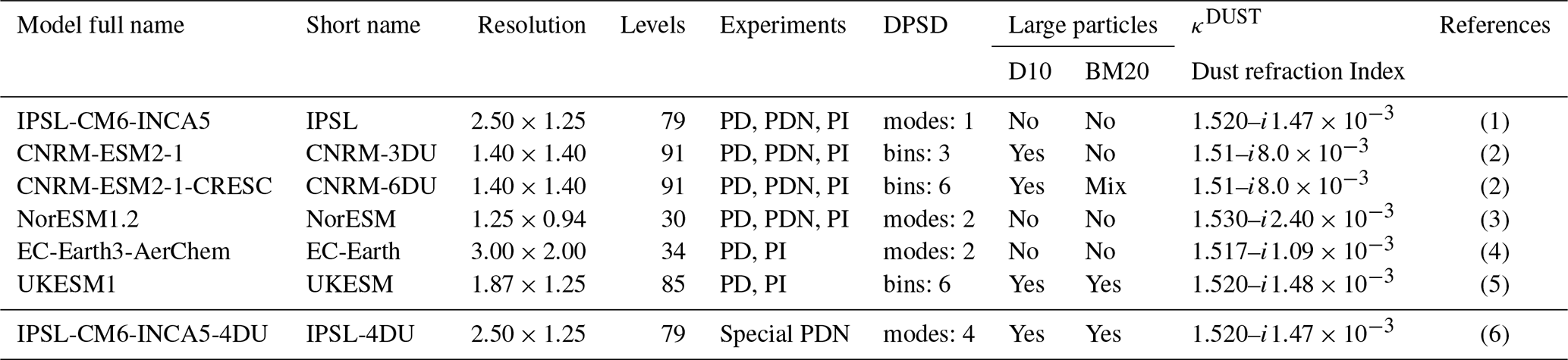
Dust scheme description: (1) Schulz et al. (1998), (2) Michou et al. (2020), (3) Zender et al. (2003), (4) Tegen et al. (2002), (5) Woodward (2001), (6) Albani et al., 2020, 2021. Earth system model description: (1) and (6) Boucher et al. (2020), (2) Séférian et al. (2019), (3) Kirkevåg et al. (2018), (4) van Noije et al. (2020), (5) Sellar et al. (2019), Mulcahy et al. (2020).

Detailed comparisons between observations and models indicate that the latter are not yet capturing the full dust spatial and temporal distribution in terms of its various properties. This is due to the fact that current Earth system models are limited to approximate phenomenological descriptions of dust mobilisation (Zender et al., 2003). These dust emission schemes are based on either a saltation process (Marticorena and Bergametti, 1995) or a brittle fragmentation model (Kok, 2011), but in both cases the momentum transfer between the wind in the boundary layer and the soil particles is conditioned by erodibility or surface roughness parameters, which are sometimes simply scaled to be in agreement with observations of aerosol index and/or aerosol optical depth. These constraints allow the models to reproduce the dust optical depth reasonably well (Ridley et al., 2016) but cannot fully constrain the whole range of the dust particle size distribution. This explains the considerable differences in surface concentrations and vertical deposition fluxes when global models are evaluated against dust observations at regional and local scales. These challenges increase in regions with strong seasonal cycles and sparse vegetation cover that require a description of the evolving vegetation, like the Sahel or semi-arid regions. Other difficulties emerge when the anthropogenic component of atmospheric dust has to be ascertained, as it requires land use change and agricultural activities to be considered. Optical properties of mineral dust aerosols are another field of research as both the refractive index and the particle shape introduce uncertainties in the estimation of scattering and absorption properties (Nousiainen, 2009). Finally, the total mass of mineral dust emitted to the atmosphere is mostly conditioned by a few events with intense surface winds, as the dust emission flux has a non-linear dependence on the wind speed, which models attempt to capture. Actually, the meteorological phenomena conditioning these events exhibit regional dependencies; e.g. in western Africa deep convection (Knippertz and Todd, 2012) and nocturnal low-level jets (Heinold et al., 2013; Washington and Todd, 2005) have been found to be key drivers. Recently, Yu et al. (2019) reported differences in the frequency of dust events between the Gobi (very high frequency of dust events in March and April) and Taklamakan (more than half of the events from May to September) deserts, which can be interpreted by a larger role in dust activation of the nocturnal low-level jet in the Taklamakan (Ge et al., 2016).

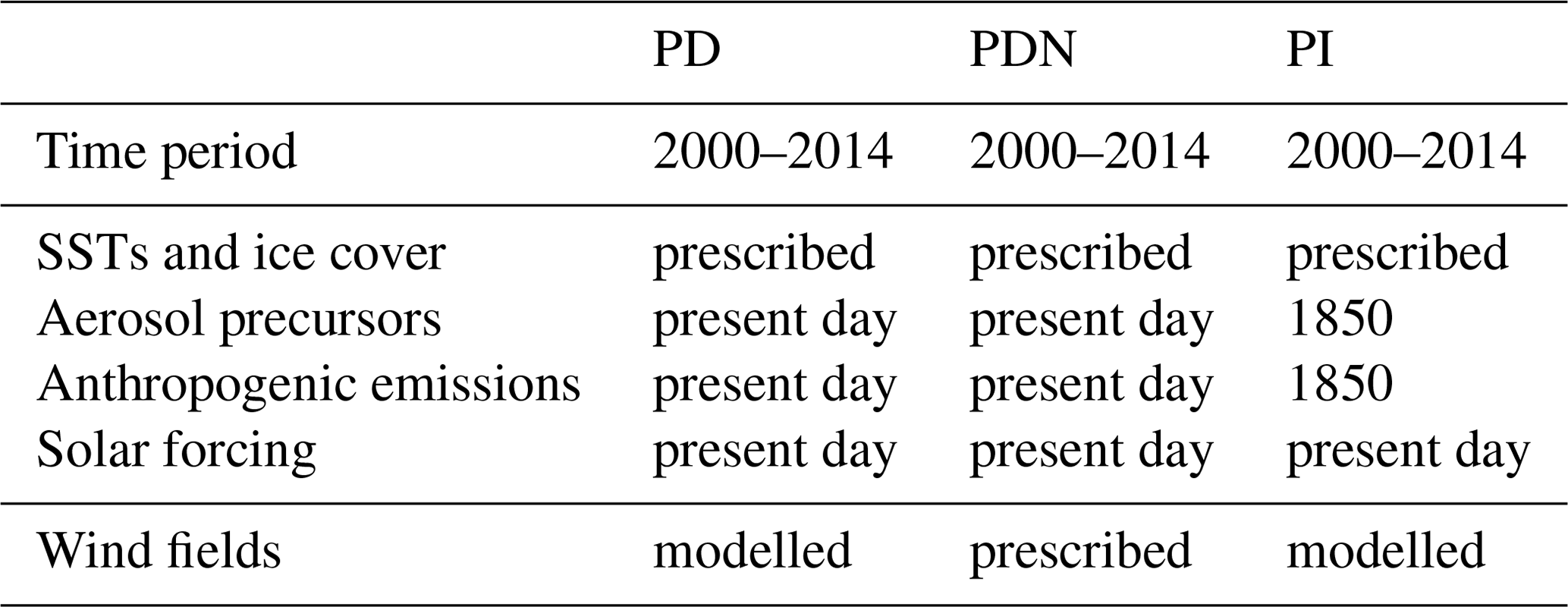
Table 2 CRESCENDO ESM experiments analysed: PD (present day), PDN (present day with nudged winds), PI (pre-industrial aerosol and chemistry forcings). The sea surface temperatures (SSTs) and ice cover are prescribed based on CMIP6-DECK-AMIP (Durack and Taylor, 2018). The solar forcing uses the input4MIPs dataset (Matthes et al., 2017), but NorESM uses the previous dataset. The gas and aerosol emissions are consistent with CMIP6,but depending on the complexity of the gas-phase species, ozone can be prescribed with either ozone concentrations from a previous full chemistry simulation or the input4MIPs ozone forcing dataset (Checa-Garcia et al., 2018; Hegglin et al., 2016). Wind fields used for the specified dynamics are obtained from reanalysis of ERA-Interim (Dee et al., 2011).

The relevance of dust in the Earth system implies that most climate models have introduced parameterisation schemes to properly describe the dust cycle in the last 2 decades. Woodward (2001) describes the parameterisation implemented in the Hadley Centre climate model, Miller et al. (2006) introduce the NASA Goddard dust model, and Schulz et al. (1998) and later Schulz et al. (2009) show the implementation of dust emissions in the INteraction of Chemistry and Aerosols (INCA) module of the IPSL model. Pérez et al. (2011) describe the BSC-DUST model, and more recently other models have either incorporated new dust schemes or improved on previous ones; e.g. Albani et al. (2014) and Scanza et al. (2015) in the CAM climate model, LeGrand et al. (2019) for the GOCART (Goddard Chemistry Aerosol Radiation and Transport) aerosol model, Klingmüller et al. (2018) in the EMAC atmospheric chemistry–climate model, Colarco et al. (2014) in the NASA GEOS-5 climate model, and Astitha et al. (2012) and Gläser et al. (2012) in the ECHAM climate model. Therefore, comparisons to ascertain how the models are improving the description of dust-related processes are needed to make progress in the above challenges. A broad comparison of 15 AeroCom models (including both climate models and chemistry transport models) in terms of dust has been conducted by Huneeus et al. (2011), and more recently there has been a comparison of dust optical depth in 7 CMIP5 (Coupled Model Intercomparison Project phase 5) climate models (Pu and Ginoux, 2018b). Albani et al. (2014) show a detailed comparison of several dust schemes of the CAM climate model. However, as the evolution of ESMs and dust schemes continues, in parallel with the availability of longer and new and/or refined observations, exhaustive comparisons of dust cycle modelling, covering scales from the global to the local, are still needed.

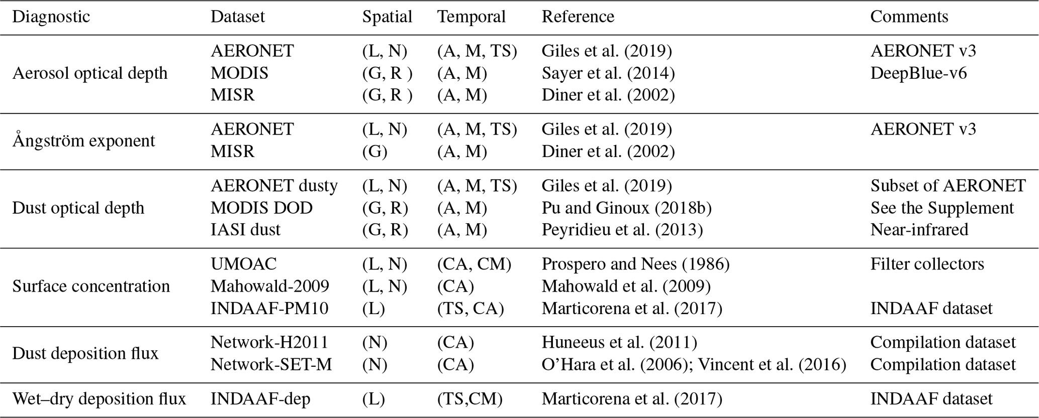
Giles et al. (2019)Sayer et al. (2014)Diner et al. (2002)Giles et al. (2019)Diner et al. (2002)Giles et al. (2019)Pu and Ginoux (2018b)Peyridieu et al. (2013)Prospero and Nees (1986)Mahowald et al. (2009)Marticorena et al. (2017)Huneeus et al. (2011)O'Hara et al. (2006); Vincent et al. (2016)Marticorena et al. (2017)

Table 3 Observations used for the comparison of the CRESCENDO models against observations indicating the spatial and temporal scales considered. Loadings and mass extinction efficiency (MEE) were derived from model results only and are compared between them. L: local, N: network, G: global, R: regional, A: annual, M: monthly, CM: monthly climatology, CA: annual climatology, TS: time series available.

This study aims to carry out an extensive comparison between observations and five Earth system models from the Coordinated Research in Earth Systems and Climate: Experiments, kNowledge, Dissemination and Outreach (CRESCENDO) project, which aims to develop the current European ESMs through targeted improvements to a range of key processes, in particular natural aerosols and trace gases. We compare the ESMs against observations in terms of optical properties (dust optical depth, Ångström exponent), surface concentration, wet and dry deposition, and dust emissions, as well as how these aspects evolve in time and space. The paper is structured as follows: Sect. 2 describes the models analysed, which is followed by Sect. 3 describing the observational datasets used and the methods (Sect. 4). The results of the comparison are presented first at the global scale (Sect. 5.1), also showing its climatological spatial patterns (Sect. 5.2), followed by sections describing dust emission (Sect. 5.3), dust deposition (Sect. 5.4), dust optical depths (Sect. 5.5) and surface concentrations (Sect. 5.6). These results are then discussed in Sect. 6 where the main conclusions are also summarised. Our final summary of future research recommendations is in Sect. 7. The Supplement is a single document but organised according to the sections of the main paper: the Supplement MD has additional information in Sects. 2 (models) and 3 (datasets). The Supplement GL complements Sect. 5.1. The other Supplement parts refer to each of the diagnostics analysed.

2 Model description

Five different Earth system models (Table 1) constitute the CRESCENDO ESM ensemble: CNRM-ESM2-1, NorESM1.2, EC-Earth3-AerChem, IPSL-CM6-INCA5 and UKESM1, with two different dust schemes for CNRM-ESM2-1 and IPLS-CM6-INCA5 (hereafter we refer to each model by the short names in Table 1). This ensemble covers the two main methods to describe the dust particle size distribution: binned–sectional and multi-modal log-normal.

In the sectional methodology the full size distribution is divided into a fixed number of bins, while inside each bin the size distribution is considered invariant. For CNRM-ESM2-1 two different dust schemes based on two different sets of bins have been evaluated (see Table S.MD.8 for further details), named CNRM-6DU (with six bins) and CNRM-3DU (with three bins). The UKESM includes six bins, with both UKESM and CNRM-6DU also covering particles with diameters larger than 20 µm, two bins in the case of the UKESM and one bin in the case of the CNRM-6DU model.

In the case of modal description the evolution of the size distribution is controlled by balance equations of mass and number concentrations of each mode, as they effectively constrain a log-normal distribution with fixed width. In CRESCENDO there are two main approaches: EC-Earth and NorESM consider bimodal size distributions (with one fine–accumulation mode and one coarse mode) mixed with other aerosols, whereas IPSL considers an externally mixed single dust coarse mode (see Table S.MD.9). The limit between coarse and fine particles is located at about 1 µm (while accumulation refers to fine particles from 0.1 to 1 µm). Denjean et al. (2016) aimed to estimate the typical parameters of a multi-modal description of the dust size distribution but confined to the range of sizes typical of accumulation and coarse modes. Recent experiments have also included larger particles (Ryder et al., 2018, 2019). A new analysis by Adebiyi and Kok (2020) proposes that the coarse mode, more specifically particles with diameters larger than 20 µm, is important to better understand the global dust cycle (often referred to as super-coarse and giant dust particles). Therefore, we also compared the CRESCENDO ESM modal dust schemes with a new dust scheme of the IPSL model with four insoluble dust modes whose properties are based on the FENNEC campaign (Rocha-Lima et al., 2018; Di Biagio et al., 2020). Table S.MD.9 shows the modal approaches in CRESCENDO and how they compare with IPSL-4DU.

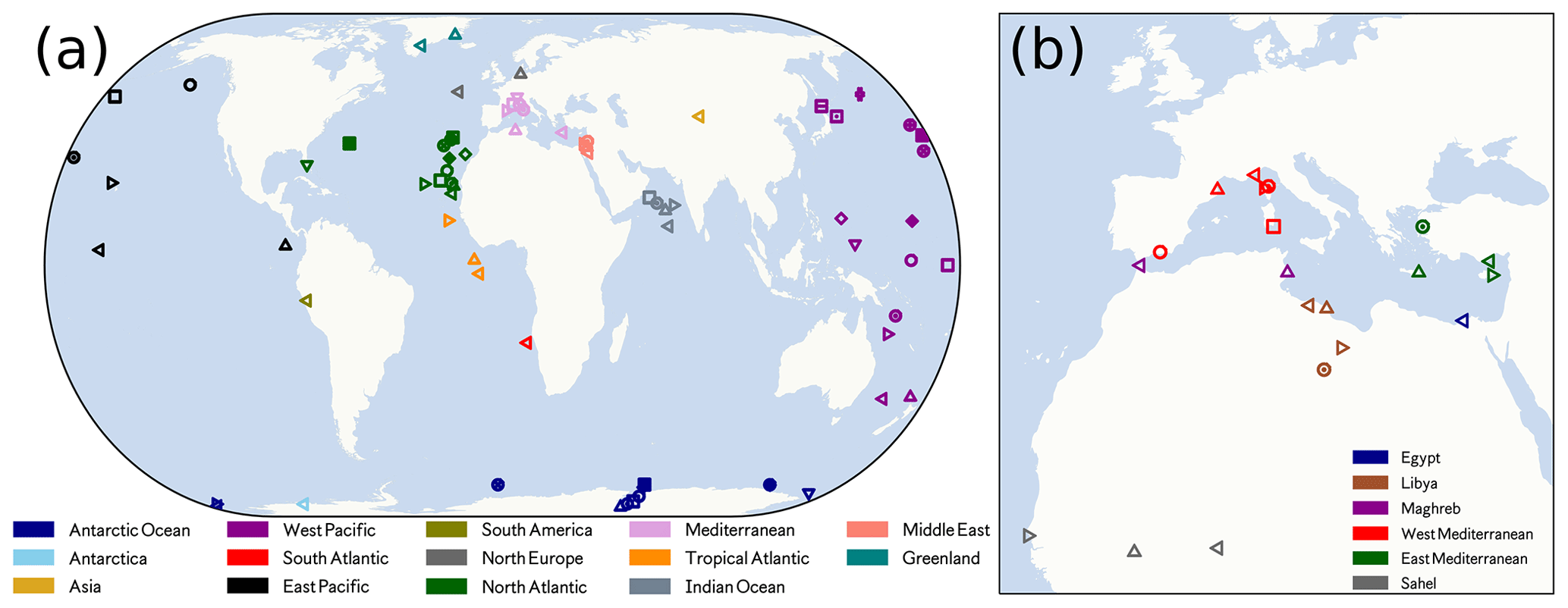
Figure 1 (a) Map with the stations of the dataset named Network-H2011, which collects annual dust deposition fluxes for multiple years (Huneeus et al., 2011). (b) Map with the stations of the dataset named Network-SET-M, which collects additional station data in the Mediterranean region where observations have been reported by O'Hara et al. (2006) and Vincent et al. (2016), as well as station data over the Sahel (Marticorena et al., 2017). The different colours represent the region where each station is located.

To better describe the CRESCENDO ensemble diversity in the modelling of the coarse mode (large particles), two classifiers are introduced in Table 1: one to differentiate dust schemes that aim to include particles with diameters larger than 10 µm and the other one to indicate whether the model explicitly has a bin or mode for particles with diameters larger than 20 µm.

All the models provide standard approaches that estimate dust mobilisation based on a velocity threshold, information on soil texture (clay–silt), erodibility factors (including soil moisture or accumulated precipitation) and prescribed vegetation cover. Conceptually, a fraction of the horizontal flux of dust particles, dominated by sandblasting, is actually transformed into a vertical flux with a mass efficiency factor and then effectively transported by the atmosphere. EC-Earth emissions are calculated following the scheme described by Tegen et al. (2002) based on the horizontal dust flux proposed by Marticorena and Bergametti (1995), which is also used in the UKESM dust scheme (Woodward, 2001). The NorESM emissions are estimated with the Dust Entrainment And Deposition (DEAD) model (Zender et al., 2003). The IPSL dust emission has been described by Schulz et al. (2009, 1998), and the CNRM-3DU model (Nabat et al., 2012) also used Marticorena and Bergametti (1995) with an emitted size distribution based on Kok (2011), while CNRM-6DU is a revised version of the CNRM-3DU dust scheme.

Although none of the models have implemented an explicit mineralogical description of dust particles, the optical refractive index effectively accounts for the global average of the mixture of minerals present in the mineral dust aerosol. Therefore, those optical properties are representative for the global mineralogical composition rather than a description of the soil-type dependence of the mineralogy that would imply local differences in emitted optical properties. This approximation is considered to drive specific biases in regions where the fraction of hematite or goethite minerals induces larger values of optical absorption, as shown by Balkanski et al. (2007) and Balkanski et al. (2021). The refractive index, expressed as ${\mathit{\kappa }}^{\mathrm{DUST}}=n-ki$, of each model is shown in Table 1. They have similar values for the real component, but the imaginary component, although small, can be different by a factor of 2, which implies discrepancies in mass absorbing efficiency. Beyond the refractive index, the optical model used to estimate the key optical properties is another factor of diversity.

In all the models the particle size is described by the geometric diameter; the dust particles with irregular shapes are modelled by spherical particles with the same effective volume. Optical properties are calculated based on Mie scattering; this approximation is reasonable as far as the orientation of the particles is randomly distributed, but any physical process that breaks this hypothesis, like preferential transport of specific geometries or physical processes that promote a specific orientation of the particles, will imply a bias in the methodology. The geometry of the particles also affects the gravitational settling and therefore the transport of particles with specific geometries (Li and Osada, 2007) and their lifetime in the atmosphere. Recently, Huang et al. (2020) have estimated that the asphericity increases gravitational settling lifetime by 20 % for both fine and coarse modes. Additionally, the spherical approximation is considered to underestimate the optical extinction of mineral dust (Kok et al., 2017). This hypothesis also affects the actual area of the global mineral dust surface, which is important in heterogeneous chemistry (Bauer, 2004) and influences tropospheric chemistry.

2.1 Model experiments

Because the models have interactive dust emissions, wind fields play a prominent role in dust emission and transport (Timmreck and Schulz, 2004). Therefore, this study contrasts two different present-day forcing experiments: one with winds generated by the dynamical part of the climate model (named PD) and the other nudged to reanalysed winds (named PDN) from ERA-Interim (Dee et al., 2011). The historical greenhouse gas concentrations are consistent with Meinshausen et al. (2017). The models IPSL and IPSL-4DU were run without explicit gas-phase interactive chemistry activated; therefore, they use the CMIP6 ozone forcing database (Checa-Garcia et al., 2018). The CNRM-ESM2-1 has explicit chemistry in the stratosphere and upper atmosphere (Michou et al., 2020). A last simulation wherein aerosols and chemistry emissions are prescribed for 1850 (named PI) is presented as well; see Table 2. All the simulations are from 2000 to 2014 plus at least 1 year of spin-up (except NorESM-PDN that covers 2001 to 2014). All the simulations implement prescribed sea surface temperatures (SSTs) of present-day conditions according to the input4MIPs dataset (Durack and Taylor, 2018). The solar forcing implemented by all the models is derived from the dataset of Matthes et al. (2017). The comparison between the PD and PDN experiments provides information on the role of wind fields in explaining model diversity. The difference between PD and PI dust emissions allows us to evaluate whether the effects in the climate system due to non-dust emissions have a discernible impact on the global dust cycle (as both PD and PI have been prescribed with the same SSTs). A summary of the properties of the model experiments is given in Table 2.

3 Observational datasets

The observational datasets used to assess the performance of the CRESCENDO ESMs in their representation of mineral dust are based on a compilation of ground site and satellite measurements. Table 3 summarises the different available datasets used as well as the spatial and temporal scales applied in the analysis. Additionally, this table includes datasets representative of either a monthly or a yearly climatology (respectively referred to as CM and CA in Table 3). In this section these datasets are briefly described, but we refer to the original publications for further details. For datasets with specific preprocessing additional details are given in the Supplement.

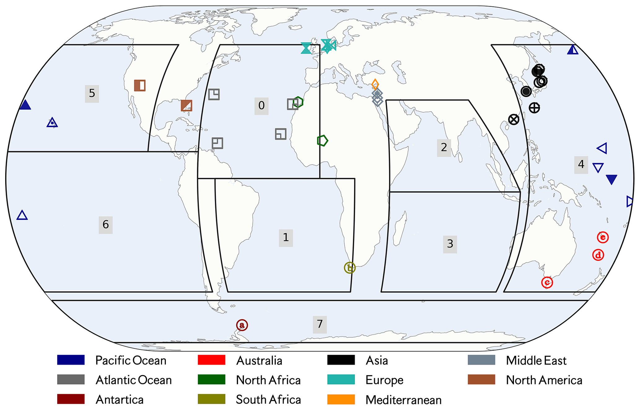
Figure 2 Map with 36 stations where surface concentrations were monitored by UMOAC (University of Miami Oceanic Aerosols Network) and also those described by Mahowald et al. (2009). Colours represent the region where each station is located. The regions correspond to those used for the regional analysis of dust deposition over the ocean: North Atlantic (0), South Atlantic (1), northern Indian Ocean (2), southern Indian Ocean (3), Pacific west (4), Pacific north-east (5), Pacific south-east (6) and Antarctic Ocean (7). For each of the oceanic regions a land mask is also applied to filter inland grid cells.

3.1 Surface deposition flux

This dataset comprises deposition flux observations described in Huneeus et al. (2011) composed of several measurement campaigns over land and ocean (Fig. 1a), hereafter named Network-H2011, plus an additional set of measurements at stations in the Mediterranean and Sahel regions (Fig. 1b), hereafter named Network-SET-M, for which data values are shown in Table S.MD.5.

The set Network-H2011 gives deposition fluxes estimated from sedimentation corresponding to the DIRTMAP (Dust Indicators and Records of Terrestrial and MArine Palaeo-environments) database (Kohfeld and Harrison, 2001), while direct measurements of deposition fluxes were acquired during the SEAREX campaign (Ginoux et al., 2001), mostly in the Northern Hemisphere. Mahowald et al. (2009) describe 28 sites where dust deposition is inferred assuming a 3.5 % fraction of iron. The compilation also includes observations of deposition fluxes deduced from ice core data according to Huneeus et al. (2011). The dataset covers a range of total dust flux deposition from 10⁻³ to 0.5×10³ $\mathrm{g}{\mathrm{m}}^{-\mathrm{2}}{\mathrm{yr}}^{-\mathrm{1}}$ but without a homogeneous distribution of values over this range. Only two stations have observational values larger than 100 $\mathrm{g}{\mathrm{m}}^{-\mathrm{2}}{\mathrm{yr}}^{-\mathrm{1}}$, and the bulk set of stations comprised values between 0.1 and 75 $\mathrm{g}{\mathrm{m}}^{-\mathrm{2}}{\mathrm{yr}}^{-\mathrm{1}}$.

The dataset Network-SET-M includes field measurements for 20 additional stations located in the Mediterranean and Sahel regions to represent deposition both near dust sources (O'Hara et al., 2006) and at intermediate distances from them (Vincent et al., 2016). The values in this dataset ranges from 4.2 to 270 $\mathrm{g}{\mathrm{m}}^{-\mathrm{2}}{\mathrm{yr}}^{-\mathrm{1}}$ and allow us to visualise regional differences in the dust deposition flux. The INDAAF (International Network to study Deposition and Atmospheric composition in Africa) stations (Marticorena et al., 2017) provide us with an estimation of the inter-annual variability, which is large in the Sahel region (see the Table S.MD.7)

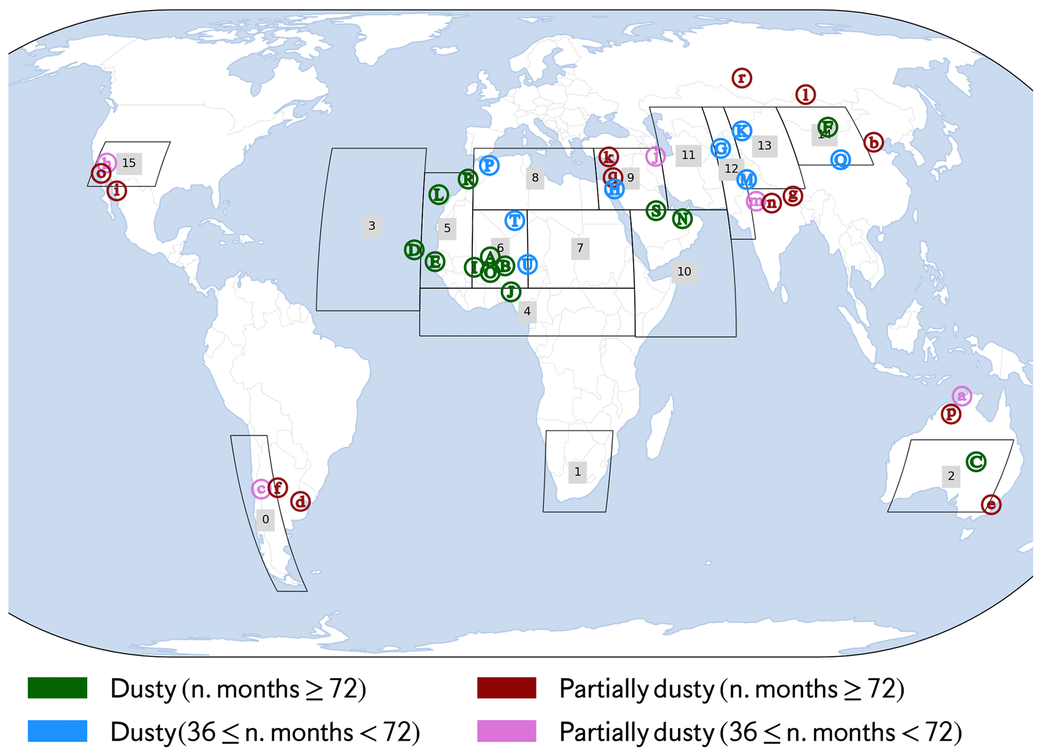
Figure 3 Map showing the 39 dusty stations from AERONET classified in two groups: 21 dust-dominated stations (uppercase letters) and 18 stations where dust is important but not necessarily dominant (lowercase letters). The colour allows also differentiating the number of months in the observed time series. The regions for the preferential dust emission sources (plus the mid-Atlantic region) are indicated by numbered boxes. The region number corresponds to the name of the region in which they are located: South America (0), southern Africa (1), Australia (2), mid-Atlantic (3), Gulf of Guinea (4), western Sahara (5), Mali–Niger (6), Bodélé–Sudan (7), northern Sahara (8), northern Middle East (9), southern Middle East (10), Kyzyl Kum (11), Thar (12), Taklamakan (13), Gobi Desert (14), North America (15).

3.2 Surface concentrations

The first part of the climatological dataset for dust concentrations (see Table S.MD.4) at the surface has been adopted from estimations done by the University of Miami Oceanic Aerosols Network (UMOAN) whose instruments are filter collectors deployed in the North Atlantic and Pacific oceans (Prospero and Nees, 1986; Prospero and Savoie, 1989). This dataset provides climatological monthly averages with a standard deviation that represents inter-annual variability. The second part of the climatological dataset is based on yearly values from the station data shown in Mahowald et al. (2009). The dataset comprises 36 stations with values from $\mathrm{5}\times {\mathrm{10}}^{-\mathrm{2}}$ to 100 µg m⁻³ distributed within the full range of values but grouped in clusters correlated with the geographical regions they belong to.

Table 4 Given here are the mass mixing ratios X_s, air mass a_mass, optical depths τ_s per species s and air density ρ_air. We indicate the method used to estimate other diagnostics; i and j are the coordinates and index of each cell grid, and l represents the level and layer. A(i,j) is the area of (i,j) grid cell, and l₀ represents the surface layer. The units refer to those of original CRESCENDO diagnostics.

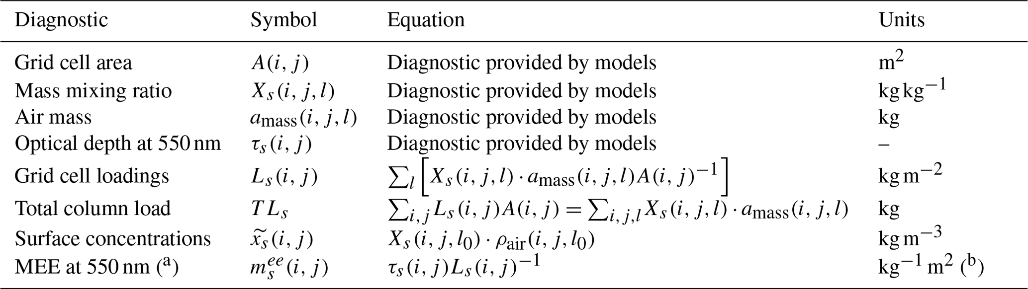
^a MEE: mass extinction efficiency. ^b The MEE shown in the analysis has units g⁻¹ m² = ${\mathrm{10}}^{-\mathrm{3}}{\mathrm{kg}}^{-\mathrm{1}}{\mathrm{m}}^{\mathrm{2}}.$

3.3 INDAAF stations of data

The multi-instrument network was deployed in the framework of the African Monsoon Multidisciplinary Analysis and belongs to the INDAAF set of data stations. Marticorena et al. (2010) described the collocated measurements of wet and dry deposition as well as surface concentrations (of particulate matter smaller than 10 µm) at three stations in the Sahel region; see Tables S.MD.6 and S.MD.7 and Fig. 1b. The stations also measured precipitation, wind velocity and surface temperature. Additionally, in the same locations there are AERONET sun photometers to measure aerosol optical depths.

3.4 AERONET optical properties

The AERONET (aerosol robotic network) database implemented in our comparisons relies on the version 3 (level 2.0) algorithm. Based on this new algorithm the entire database of observations was reprocessed in 2018 (Giles et al., 2019). The database comprises aerosol optical depths and Ångström exponents, as well as fine and coarse optical properties obtained with a new cloud-screening quality control scheme. The actual division threshold between fine and coarse particles is ascertained by the inversion algorithm that aims to differentiate aerosol particles from ice crystals, and it lies between 0.44 and 0.99 µm.

The network database provides daily data, allowing for event analysis, and there is also a monthly time resolution dataset used here to examine decadal, yearly and seasonal properties. We processed data from 300 stations of the full network to explore general properties. For the dust analysis we selected stations where all the models together considered dust to be an important contributor to the aerosol composition (at the geographical location of the AERONET station). This subset is called the dusty set of stations here, which are shown in Fig. 3. It comprises 39 stations divided into two subsets: stations where the dust has a dominant role in terms of the optical depth (${\mathit{\tau }}_{\mathrm{440}}^{\mathrm{dust}}>\mathrm{0.5}{\mathit{\tau }}_{\mathrm{440}}^{\text{all-aer}}$ for all models and all the months of the year, with ${\mathit{\tau }}_{\mathrm{440}}^{\text{all-aer}}$ referring to optical depth at 440 nm of all aerosols and ${\mathit{\tau }}_{\mathrm{440}}^{\text{dust}}$ the optical depth of mineral dust aerosols at 440 nm) and those where the dust is important although not necessarily dominant for all the models (even if the dust optical depth from a single model contributes more than 50 % of the total aerosol optical depth). The first subset comprises 21 stations, and it is denoted with uppercase letters in Fig. 3. The second comprises 19 stations, and it is denoted with lowercase letters. The dusty station set over Africa is consistent with the stations analysed by Huneeus et al. (2011) based on the Bellouin et al. (2005) criteria, but it has been extended with stations in Australia, South America, North America and Asia, consistent with Klingmüller et al. (2018). Figures with the seasonal cycle of aerosol optical depth for the dominantly dusty and important stations that highlight the classification criteria are shown in the Supplement (Figs. S.DOD.10 and S.DOD.11).

Table 5 Statistic used to intercompare models and observations and perform model intercomparisons. N indicates the number of observations or sample size. When the analysis refers to a global performance of the model over a set of instruments, N represents the number of stations. When the statistical analysis is done over a time series of values, N represents the number of time samples usually corresponding to a specific location. The equations include the Pearson correlation coefficient (ρ), bias (δ), normalised bias (δ_N), ratio of standard deviations (Σ), normalised mean absolute error (θ_N) and root mean square error (RMSE =η).

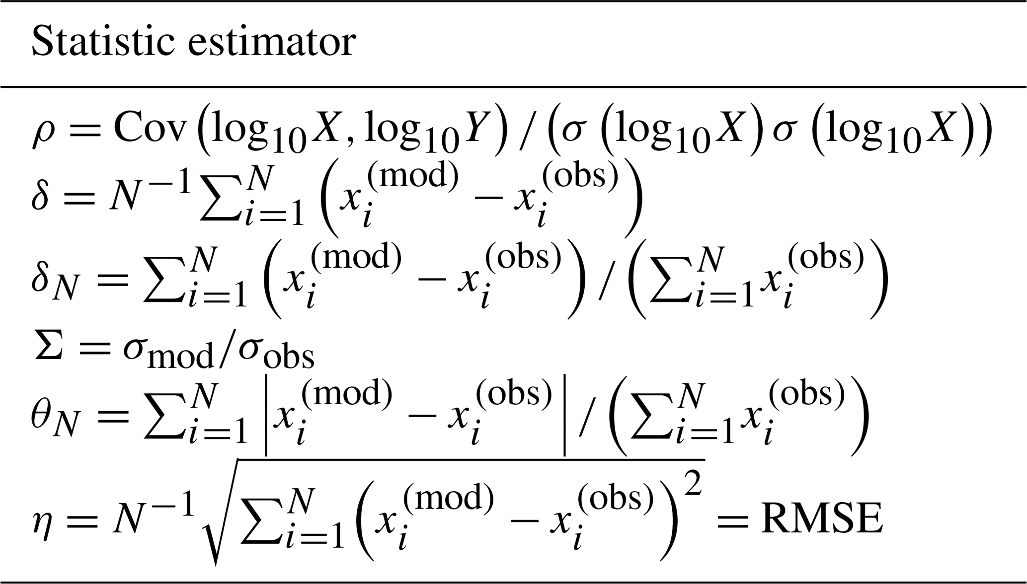
Table 6 Global dust mass balance, dust loading, dust optical depth (DOD), mass extinction efficiency (MEE) and lifetime for each model and each experiment available. CNRM has two configurations: one specific for CRESCENDO referred to as CNRM-6DU and another for CMIP6 denoted as CNRM-3DU. The UKESM does not diagnose the dust sedimentation separately, and dry deposition flux diagnostics account for all removal of dust except for wet deposition. The units are Tg yr⁻¹ for emissions and deposition tendencies, Tg for load, m² g⁻¹ for MEE, and days for lifetime. MEE is calculated as the mean of the MEE(x,y) field, while $\widehat{\mathrm{MEE}}$ is the ratio of DOD and load mean fields. Δ represents the ratio of the net (emission–total deposition) relative to emissions in percent (%). ℛ_dep is the ratio of total dry (including gravitational settling) over total wet deposition. MM-mean shows the multi-model mean for each experiment (and each variable) and MM-σ the estimated multi-model standard deviation. Note that some statistical estimations (indicated with ^b) related to the deposition do not include the UKESM as we cannot separate gravitational settling from other dry deposition processes. Due to the larger values of the Δ parameter, CNRM-6DU is not included in the statistics marked with ^c and ^b.

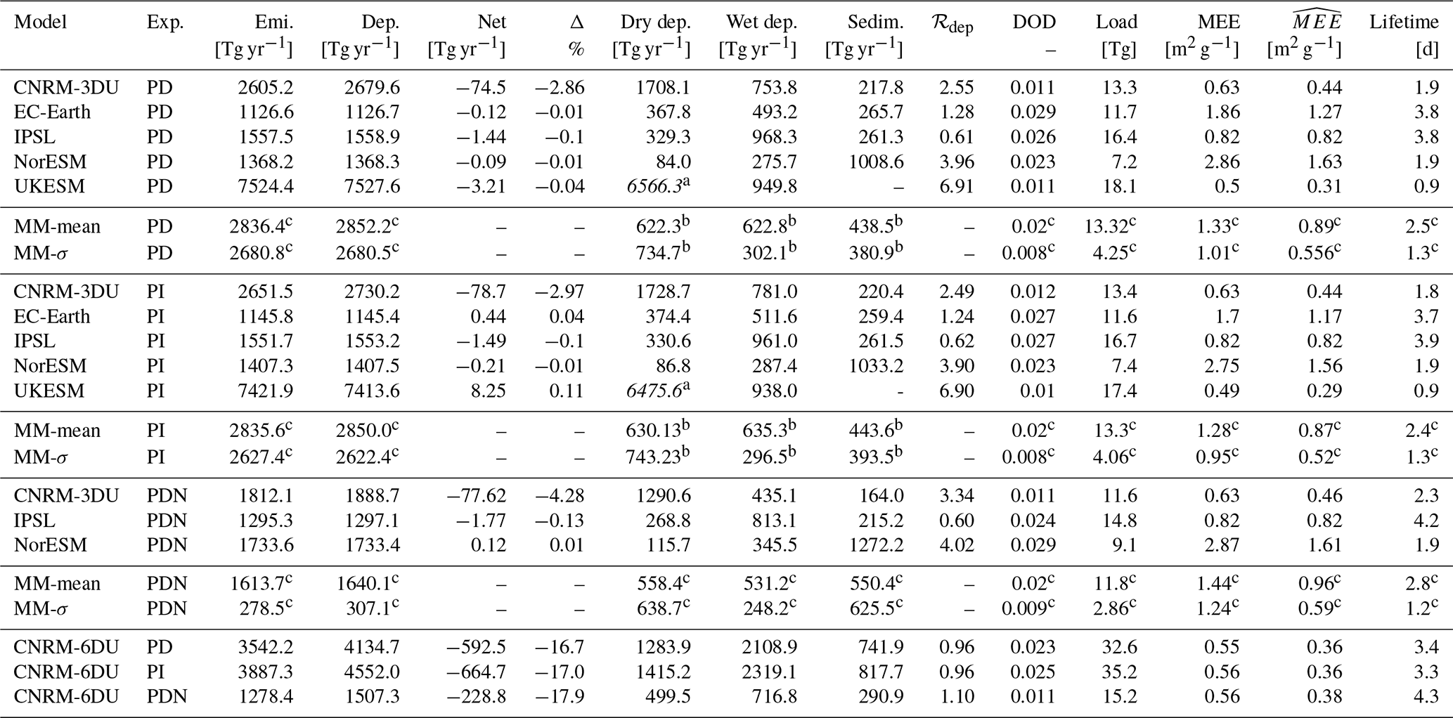
^a Values including the sedimentation. ^b Statistic does not include UKESM and CNRM-6DU. ^c Statistic does not include CNRM-6DU.

3.5 MODIS dust-related products

Interactions between dust and radiation are defined through three optical properties: dust optical depth (DOD), single-scattering albedo (ω) and the asymmetry parameter, which defines the ratio of the radiation scattered forward over the radiation scattered backward. For the dust coarse mode, the dust optical depth can be estimated using the Moderate Resolution Imaging Spectroradiometer (MODIS) enhanced deep-blue (DB) aerosol optical depth (Sayer et al., 2014) as done by Pu and Ginoux (2018b) with the additional support of the MODIS product of single-scattering albedo (ω) and Ångström exponent (α). The rationale of the method relies on the properties of these three optical parameters applied to aerosol particles. First, α is very sensitive to particle size, so there are parameterisations of aerosol optical depth that use it to separate each mode contribution. Second, aerosols with low absorption and large scattering like sea salt have ω≃1, whereas mineral dust is considered an absorbing aerosol. Third, the dependency of α(λ) on wavelength contains a signature of the aerosol composition. Given this information, we have considered two different MODIS dust-optical-depth-related datasets. One of them is a pure filter of aerosol optical depth to differentiate pixels wherein dust is expected to be the dominant contribution to aerosol optical depth, but without an attempt to estimate the actual fraction of mineral dust, so it is considered here to be an upper threshold for the actual DOD of the coarse mode (because particles of dust with diameters below 1 µm are thought to contribute less than 10 % to the total dust optical depth). The other method aims to explicitly separate sea salt and proceeds to rescale the aerosol optical depth to ascertain an actual value of DOD; according to Pu and Ginoux (2018b) it may be considered a lower bound for the DOD. Additional information and a comparison of these created products are given in the Supplement; see Figs. S.MD.2 and S.MD.3.

3.6 MISR aerosol-optical-depth-derived products

The Multi-angle Imaging Spectroradiometer (MISR) is a sensor on board the Terra satellite which takes advantage of its multi-angle measurement capabilities. It is able to ascertain the presence of non-spherical particles in the aerosol products at four different wavelengths. The optical depth at several wavelengths has been used to compute the Ångström exponent between March 2000 and December 2014 from MISR and compare with the models' Ångström exponent based on the same information. This product gives us information on how the models represent the spectral dependence of optical depth. Our computation using the 446 and the 672 nm wavelengths has been compared with the MISR Ångström exponent product to validate our computations; see Fig. S.GL.8.

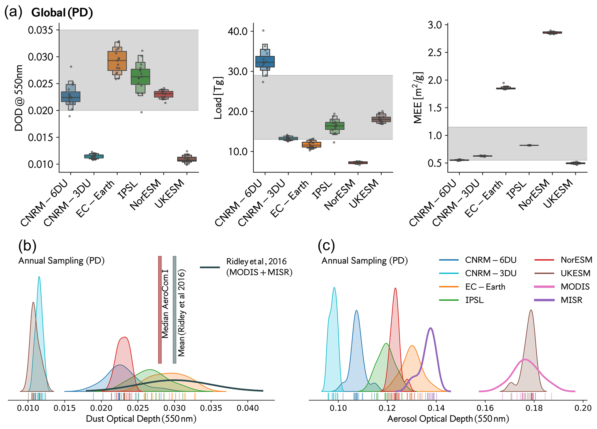
Figure 4 (a) Global dust cycle values for the PD experiment. The grey shaded region represents the expected interval range based on Kok et al. (2017) for dust particles with a diameter up to 20 µm for dust optical depth (DOD), load and mass extinction efficiency (MEE). The grey dots over the box plot represent each of the annual values. (b) The estimated distribution of global dust optical depth annual values (our sample values per model are represented by the coloured vertical marks just above the x axis). (c) The analogous distribution for the optical depth of all aerosols. Both distributions are normalised, and the vertical axis represents a probability. For both the models and the observations (MISR and MODIS) the estimates are for time period 2000–2014. Additional analyses analogous to the top panel but constrained over different regions are in the Supplement (Figs. S.GL.1 and S.GL.2).

4 Methods

As part of this study we calculated several diagnostics not directly provided by the different models. Table 4 shows how they have been estimated together with their units. Regarding the statistical methods, Table 5 shows the metrics used for the comparison of the CRESCENDO models with the comprehensive suite of observations. The skill of the models to represent the dust optical depth over dust source regions has been calculated based on the Pearson correlation. Given that this statistic is not robust because of its instability in the presence of outliers (Li et al., 2006) and is only representative of linear relationships, the skill is also estimated based on the Spearman rank correlation to ensure the robustness of the results. For the other comparisons beyond the skill, the scatterplots are informative of the quality of the Pearson correlation estimator.

For the comparison against the networks of instruments used (one monitoring surface concentrations, two for total deposition and one that retrieves dust optical depth), we proceed with the same methodology. For each observation, we chose the model value of the corresponding variable in the grid pixel to which this measuring station belongs. Given the different area covered by the grid cell and the grid point location of the in situ measurements, there is an underlying representation error. However, the observational datasets of total deposition and surface concentrations at point-based sites are climatological estimations which can be representative of larger areas. The values for the parameters discussed here are time-averaged over the 15-year simulations, and hence the produced fields are smooth over sub-grid scales.

The surface concentration and total deposition comparisons are presented as scatterplots together with three associated statistics: the Pearson correlation (evaluated in log scale), the bias and the RMSE (root mean square error). These last two metrics can be used to characterise quantitative differences between each model and the observations. Additional statistics are summarised in Tables 11, 12 and 13 including the normalised bias and the normalised mean absolute error, which help us understand how the models differ when scaled to the observation values.

5 Results

The results are divided into six different subsections. First a comparison at the global scale summarises the main properties of the global dust cycle in the models analysed, which is complemented by an overview of the spatial pattern of the temporal mean of the 15 years of simulation (based on monthly values) for each of the climate models in the study. The next four sections give a detailed analysis of the dust properties: emission, deposition, optical depth and surface concentrations. Each one is described at the regional scale and compared against a network of instruments and/or satellite retrievals when available. In all the cases, the PD experiment simulations have been taken as the baseline of the intercomparison and shown in the main paper. The results for the other experiments (PDN and PI), if not present in the main paper, are shown in the Supplement. The case of nudged wind simulations (PDN) is used to ascertain the role of modelled surface winds in inter-model differences, whereas the simulation with PI emissions helps us to evaluate the possible role of prescribed emissions.

5.1 Global dust properties

The global dust cycle has been analysed in terms of global climatological values and complemented by a study of the role of the particle size distribution in the direct radiative effects (based on the IPSL model with four dust modes).

The dust particle size distribution is physically constrained by emission, transport and deposition (wet and dry), whereas other aerosol processes like aerosol nucleation, condensation and coagulation have a minor role in the evolution of the size distribution (Mahowald et al., 2014). Therefore, the first step to describe the global atmospheric dust cycle in climate models consists of a characterisation of the emission and deposition fluxes at the surface. This analysis is complemented by the analysis of two size-integrated properties: the dust optical depths and loadings. Other phenomena present in the Earth system dust cycle more relevant for paleoclimate studies, like those derived from the stabilisation of dust deposition on the surface on long timescales, are not considered in this work.

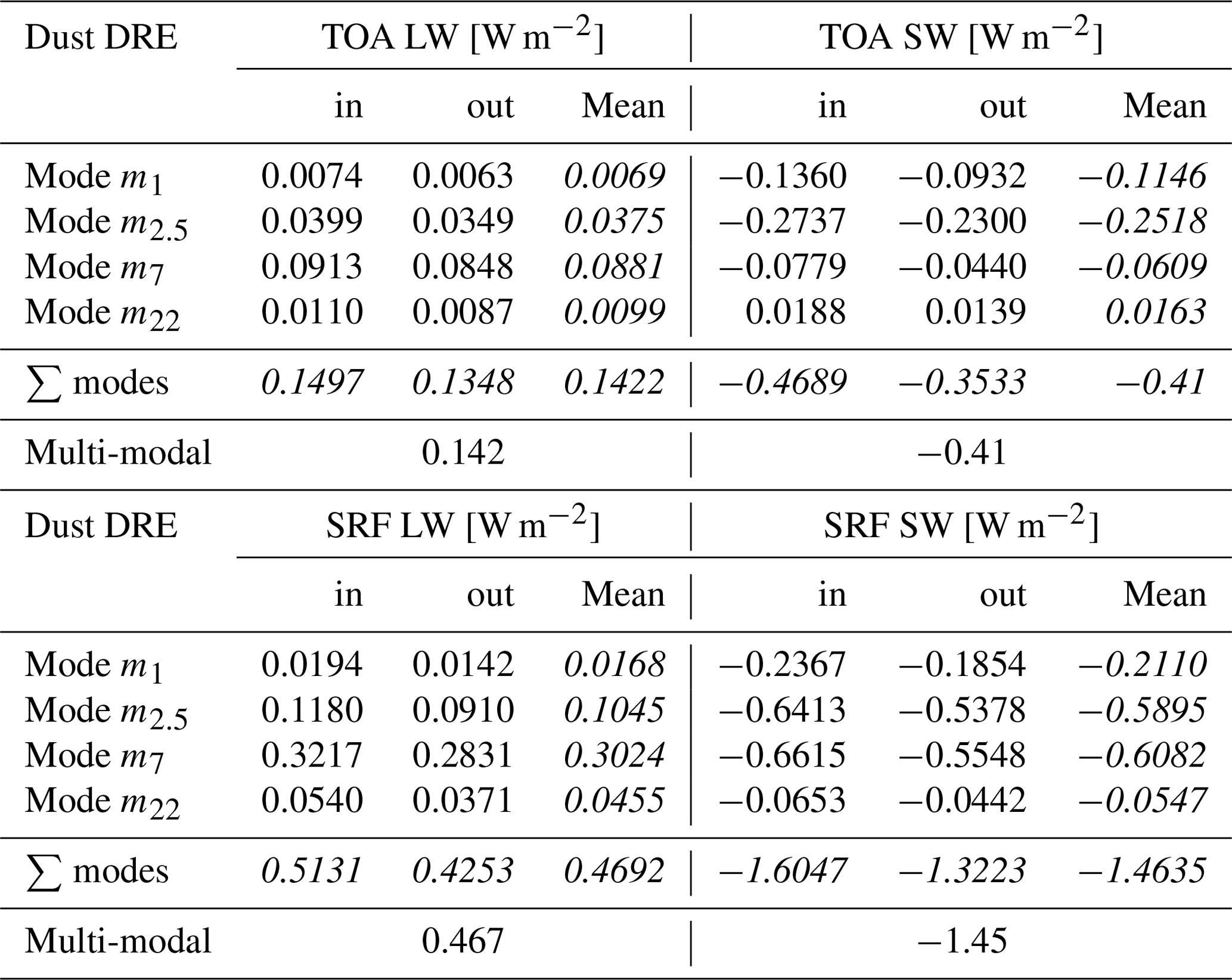
Table 7 Direct radiative effects (DREs) at the top of the atmosphere (TOA) and the surface (SRF) without clouds in the longwave (LW) and shortwave (SW) for the IPSL model with four dust modes as described by (Samuel Albani, personal communication, 2021). For each mode the value from each method in and out as well as their mean value (of both methods) are indicated (the mean value is in italics). Both methods are described in the Appendix A; the method in adds each specific mode to a case without any mode of dust, and the method out removes that specific mode to a case with all the modes of dust. Values in italics represent those derived from other values of the table. The value of the sum of the four modes is not equal to the value of the multi-modal DRE of dust for each method in or out individually. But the mean of both methods (in and out) is consistent with the multi-modal DRE.

The global dust budget is analysed for the whole time period of the simulations over the three different simulations considered: PD, PDN and PI. Table 6 presents the mean global values of each model. It describes the dust mass balance in terms of emission as well as dry and wet deposition. A parameter ℛ_dep is defined to represent the ratio of total dry to total wet deposition. In addition, Δ represents the fraction (%) of the emissions not deposited relative to the total emission. This last parameter is used to ascertain if the dust cycle from emission to deposition is consistent in terms of global mass conservation or, on the contrary, whether the model transport introduces any inconsistency in the modelled dust cycle. In particular, the parameter Δ is used to identify the models and experiments that will be included in the multi-model ensemble mean to ensure internal consistency in the ensemble.

Figure 5 CRESCENDO ESM global maps describing dust properties (averaged over 15 years): emission tendency, deposition tendencies, dust optical depth and mass extinction efficiency. The models included have a bin-based dust parameterisation; these models are CNRM-6DU, CNRM-3DU and UKESM. The equivalent figures for the PI and PDN experiments are shown in the Supplement: Figs. S.GL.3 and S.GL.4, respectively.

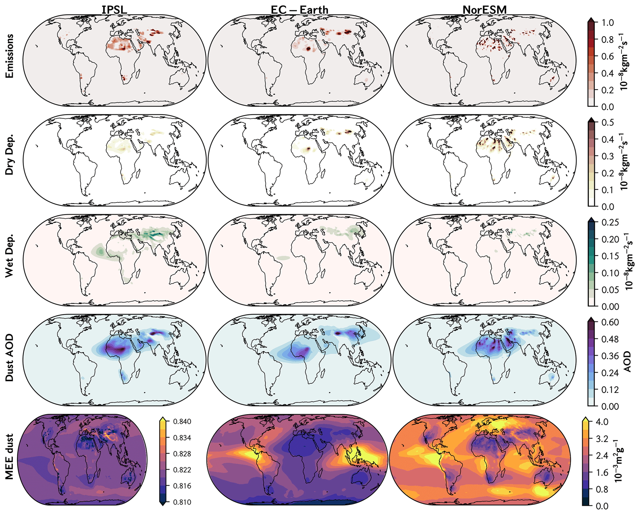
Figure 6 CRESCENDO ESM global maps of dust properties (averaged over 15 years): emission tendency, deposition tendency, dust optical depth and mass extinction efficiency. The models included have a modal-based dust parameterisation; these models are IPSL-INCA, NorESM and EC-Earth. The equivalent figures for the PI and PDN experiments are shown in the Supplement: Figs. S.GL.5 and S.GL.6, respectively.

In this regard, the mass budget of the CNRM-3DU model is closed to within Δ≃3 % as its dynamical core is based on a semi-Lagrangian method (Voldoire et al., 2012, 2019), which is not fully mass-conservative in terms of its tracers. In the case of the PDN experiment there is an increase to Δ≃4.3 % because the excess of mass in the deposition with respect to the emissions is similar for all the experiments, but the emissions of CNRM-3DU decrease with nudged winds by 30 %. The deposition value is therefore biased by an approximately constant amount of 75 Tg yr⁻¹ independently of the wind field. Given in any case the value of Δ<5 %, we have included the CNRM-3DU model in the ensemble means. In the case of the CNRM-6DU model the consequences of its dynamical core properties are the same; hence, there is also a bias. However, it is close to 600 Tg yr⁻¹ in total deposition, producing a value of Δ larger than 15 %. Therefore, this model is not included in the ensemble means. In both cases (the CNRM-3DU and the CNRM-6DU models), the bias in total deposition implies an excess of mineral dust in the atmosphere not consistent with the actual modelled emissions. A further complication is that the bias leads to other biases in variables like concentrations, load and optical depths. For this reason the CNRM-6DU model is not used in our analysis to draw conclusions about the dust cycle. But it is kept in the other analyses to be compared with future developments of the model that improve or fix the mass conservation and subsequently better highlight the implications of these kinds of numerical instabilities in dust modelling. For the other models, Δ<0.1 %, with NorESM and EC-Earth presenting values closest to zero.

The multi-model mean global emissions for the PD and PI simulation experiments are 2836 and 2835 Tg yr⁻¹, respectively, with standard deviations of 2680 and 2627 Tg yr⁻¹. The PDN experiment shows an ensemble mean value of 1614 Tg yr⁻¹, which is significantly smaller because of the models included (see Table 1), but also because of an important decrease in the CNRM-3DU total emissions. Indeed, the decrease in emissions with nudged winds is even higher in CNRM-6DU. As a consequence, our ensemble mean value for the PDN experiments agrees well with recent estimations (Kok et al., 2017) when large particles (diameter ≤ 20 µm) are not included. But it also agrees well with previous estimations of 1500 Tg yr⁻¹ based on the DEAD model (Zender et al., 2003) for particles with diameters smaller than 10 µm. At the same time, when nudged winds are used (PDN ensemble), the standard deviation of total emissions (278 Tg yr⁻¹) is significantly smaller than for the PD or PI cases. For the PD experiment, the multi-model ensemble mean total emission, for the same models as available for PDN, has a mean value of 1843 Tg yr⁻¹ with a standard deviation of 544 Tg yr⁻¹, which is significantly larger than the standard deviation of the PDN experiment. Therefore, nudged winds decrease model diversity in terms of global emissions. Indeed, the CNRM-6DU and CNRM-3DU models have total emissions with nudged winds similar to the CRESCENDO ESM ensemble mean, but they produce higher emissions without nudged wind fields, i.e. 2600 Tg yr⁻¹ in the CNRM-3DU model (diameters up to 10 µm) and 3500 Tg yr⁻¹ for CNRM-6DU (diameters up to 100 µm; see Table 1). These values are similar to the 3000 Tg yr⁻¹ reported by Tegen and Fung (1994) for particle sizes between 0.1 and 50 µm. Finally, due to the presence of particles with diameters up to 62 µm, the UKESM has notably higher emissions (although in this case we cannot assess the role of surface winds).

This higher value of total emissions due to large particles is not directly correlated with the modelled dust load in the atmosphere. The reason is that the lifetime of dust particles in the atmosphere depends on the size, and these large particles sediment faster. For instance, the UKESM has monthly mean global loading values close to the other models and a smaller lifetime of dust in the atmosphere (less than 12 h, a characteristic value of the largest particles). In fact, the dry deposition of larger particles for UKESM (which for this model includes sedimentation) is truly dominant, resulting in a wet deposition close to other models, like IPSL, without the largest particles modelled. In contrast, the CNRM-6DU wet deposition is 2 times larger than that of the UKESM and IPSL model in the PD simulation (with CNRM-6DU being the only model for which wet deposition exceeds total dry deposition) but close to IPSL with nudged winds. Because larger particles are deposited faster by gravitational settling, it is expected that ℛ_dep would be larger for models including the largest particles, but it is only obvious for the UKESM. For the CNRM-6DU model that is not the case. EC-Earth has double the value of ℛ_dep of IPSL, and NorESM is 6 times larger. Previously, Shao et al. (2011) reported values for ℛ_dep between 1.03 and 8.1, also uncorrelated with the size range of the dust particles modelled. The multi-model ensemble mean for total dry deposition without gravitational settling is 622 Tg yr⁻¹ for the PD experiment and 558 Tg yr⁻¹ for PDN. In the case of wet deposition, we estimated 623 and 531 Tg yr⁻¹ for the multi-model mean for the PD and PDN experiments, respectively. Despite the similar values of our ensemble mean, the standard deviation of dry deposition is more than 2 times that from wet deposition. To summarise, each of the processes (sedimentation, wet deposition and dry deposition – without sedimentation) has a similar contribution in the ensemble mean for all the experiments, but this is masking strong differences in these three properties from each of the models.

Table 8 First part of the table: emissions [Tg yr⁻¹] for the present day (PD) and their contribution fraction to the total global emissions globally, over land and over coastline pixels. ^a Models with modelled bin diameters larger than 20 µm. Sahara emissions and their percentage of total emissions are obtained from the sum of the regions of the western Sahara, Mali, Bodélé and the northern Sahara, so they do not include the Sahel. Second part of the table: emissions [Tg yr⁻¹] for present-day (PD) simulations over 16 different regions; see Fig. 3. In brackets are the order of the 10 regions with the largest emissions. The multi-model ensemble mean (MM-mean) includes the mean values ± the standard deviation for all the models and (^b MM-mean) for all the models without UKESM. In the Supplement (Sect. E), Tables E1 to E4 have the analogous information for the PI and PDN experiments. Ensemble means of emissions include CNRM-6DU.

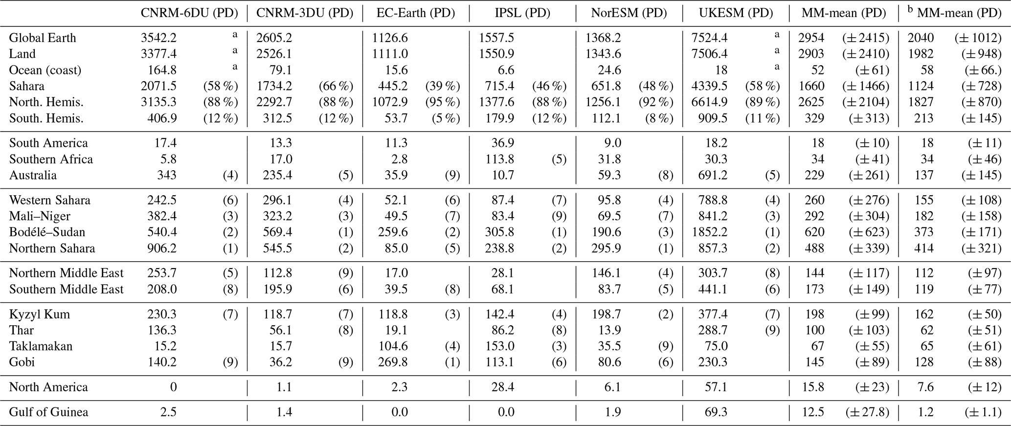
^b These statistics exclude UKESM.

As explained above, the impact of the largest particles on the global behaviour of loading and dust optical depth is considered less important than coarse particles (up to 10 µm), so this hypothesis allows us to compare all models with observational constraints that rely on optical depth measurements. Figure 4a compares the PD experiment with the Kok et al. (2017) proposed values of dust optical depth and total load. We also derive the mass extinction efficiency (MEE) field as the ratio of dust optical depth to loading field; see Table 4.

Figure 4 indicates that, aside from the CNRM-6DU model, all models have dust loadings smaller than 20 Tg, with the loading of NorESM half that of the ensemble median value. As already noted above, the load of the CNRM-6DU model is subject to a bias due to the artificial mass introduced during transport. Therefore, the set of models included in our ensemble mean (Table 6) agrees with the AeroCom Phase I models or which the fine dust dominates with a total load ensemble mean value of 15 Tg.

Also based on AeroCom Phase I, Huneeus et al. (2011) reported an MEE multi-model median of 0.72 m² g⁻¹, which is similar to the global MEE value of 0.6 m² g⁻¹ used by Pu and Ginoux (2018b) to compare DOD and dust loadings of CMIP5 models. Recently, Adebiyi et al. (2020) estimated a mean from 13 observational stations, giving a value slightly smaller than 0.6 m² g⁻¹. Our estimation of MEE shows that EC-Earth and NorESM depart from that value, whereas the other models remain reasonably close to the Pu and Ginoux (2018b) hypothesis and the AeroCom Phase I median value. The larger MEE values of EC-Earth and NorESM can be due a combination of factors: they have the lowest dust loadings and both do not model particles larger than about 8 µm. In the case of NorESM, the imaginary part of the refractive index is also the largest of all the models analysed. Our results highlight the fact that the MEE depends on the modelled dust particle size distribution (in particular the presence of large particles) but with a significantly smaller inter-annual variability than dust optical depth and loading. This fact explains its use for ad hoc relationships between dust optical depths and loadings with a constant factor (Pu and Ginoux, 2018b).

We note that the global mean values for the models, as shown in Fig. 4a, are partially influenced by ocean or land regions with low dust loadings. To complement this analysis, we present two additional comparisons in the Supplement. The first is shown in Fig. S.GL.1 for the case when only values over land are considered. The second is shown in Fig. S.GL.2 for the case when the annual values are estimated over the dust belt that covers most of the Sahara and the Middle East. Both figures still indicate important differences between models.

To further understand the properties of dust optical depth, we calculated the distribution of values for each model with a kernel density estimation based on the histogram of the annual global values of dust optical depth. The results shown in Fig. 4b indicate the presence of two main groups for our model ensemble: the first one centred around a value close to 0.01 and the second one around 0.025, which is a value closer to the proposed constraint. The solid black line shows the distribution of dust optical depth at 550 nm proposed by Ridley et al. (2016), and the vertical lines indicate the mean of that distribution and the AeroCom Phase I median value. The EC-Earth model actually agrees in terms of both the central value and typical inter-annual variability (as represented by the width of the distributions). These results should also be interpreted in the context of the total aerosol optical depth (AOD, Fig. 4c). We observe that the UKESM has the lowest values of dust optical depth but actually the largest values of total aerosol optical depth, with similar global mean values as those obtained by MODIS at 550 nm but with a narrower distribution. The EC-Earth model has AOD values slightly smaller than MISR estimates but with similar inter-annual variations. Fig. 4c indicates model discrepancies in the magnitude of the inter-annual variability (as measured by the width of the distribution) and an overall underestimation of AOD at 550 nm with respect to these satellite platforms.

A specific PDN experiment with the IPSL model was run for 5 years (2010 to 2014) to analyse how the representation of the dust size distribution influences the dust cycle. In this simulation, named IPSL-4DU, the dust scheme is based on four dust insoluble modes (m₁, m_2.5, m₇ and m₂₂; the number indicates the MMD – mass median diameter – value of that log-normal mode) covering the whole range of sizes from 0.1 to 100 µm, and nudged winds were used. The results shown in the Supplement Table S.GL.7 are consistent with the impact of larger particles on dust emissions and loadings in UKESM, and they allow us to discuss the role of each mode independently. The total emissions for IPSL-4DU are dominated by the largest particles, which are those of mode m₂₂, but are promptly removed from the atmosphere through their sedimentation, which is very rapid compared with the typical lifetime of mineral dust, as shown in Table 6. When comparing the total load for each mode, the coarse size mode m_2.5 is actually more abundant than m₂₂. Amongst all the modes, mode m₇ has the largest contribution, with $\mathrm{2}/\mathrm{3}$ of the total, which is comparable to the large particles represented in the CNRM-6DU model, consistent with Adebiyi and Kok (2020). Note that the dust loads in CNRM-6DU model are larger than in CNRM-3DU to a degree that cannot be explained solely by the larger emissions of CNRM-6DU. An explanation for this difference is that the bin that includes particle sizes from 2.5 to 20 µm in CNRM-3DU is split into different bins in the CNRM-6DU model, which have different lifetimes in the atmosphere, and that non-conservative transport could create larger aerosol mass in the CNRM-6DU configuration. In contrast to emissions, optical properties are dominated by the contributions of accumulation to coarse size particles compared to the largest particles of mode m₂₂, which does not play a large role in the contribution to aerosol extinction. Those values are then used for assessments of modal contributions to direct radiative effects.

Figure 7 Normalised map of emissions (×100) over NorESM grid resolution. On the top: experiment with present-day aerosol and chemistry forcings (PD). On the bottom: the PDN experiment. We used a conservative near-neighbour interpolation to create emission maps that preserve global values at higher resolutions; then the maps were normalised to have a common comparison scale. The colour bar represents the normalised emission tendencies per grid with the range [0,100]. Figure S.E5 is the corresponding figure for the PI experiment.

Mineral dust aerosol interaction with solar and terrestrial radiation results in both absorption and scattering of light. These interactions are strongly dependent on dust mineralogical composition and particle size distribution; hence, they differ regionally (Ginoux, 2017; Kok et al., 2017). We estimated the respective roles of the different modes (that represent different particle size ranges) and note that in the case of multi-modal distributions the estimations of direct radiative effects (DREs) by each mode are somewhat non-linear (Di Biagio et al., 2020). This is illustrated by the sum of the contribution of the DRE from each mode, which is not exactly equal to the multi-modal dust contribution. Appendix A shows how, with an estimation of DRE per mode based on the combination of two different methods, we determined modal values of DRE that, when combined, come close to the multi-modal DRE estimation. This is summarised in Table 7 where the estimates per mode of DREs for each method are shown together with their mean. The sum of these mean values per mode is now consistent with the multi-modal DRE. It is remarkable how the estimations of DRE at TOA-SW (top of the atmosphere in the shortwave) for m₇ for each method differ by a factor of 2. The non-linear effects at the surface in the SW are also important, with differences in the sum of the four modes between methods of 0.3 W m⁻².

The analysis of direct radiative effects (DREs) by mode, shown in Table 7, indicates that the largest particles (mode m₂₂) have a minor impact on the DRE in both the LW and SW according to the IPSL-4DU model. In contrast, the inclusion of the mode with the smallest particles contributes to SW cooling, although it is the coarse size mode that dominates the net direct radiative effects at the top of the atmosphere. At the surface, however, mode m₇ has the largest effect on both SW and LW, but its net contribution (LW+SW) is smaller than the coarse mode m_2.5. It is important to note that the DRE shown in Table 7 is estimated without scattering in the LW (only absorption). To neglect the LW scattering in the case of mineral dust implies an underestimation of TOA-DRE-LW (Dufresne et al., 2002), mostly in cloud conditions.

5.2 Dust global spatial patterns

A global picture of the dust cycle is shown in Figs. 5 and 6, which describe temporal mean properties of dust in CRESCENDO ESMs (PD simulations) over 15 years. The spatial resolution and vertical levels of the models are introduced in Table 1.

First, models that have a sectional representation of the DPSD (CNRM-6DU, CNRM-3DU and UKESM) are shown in Fig. 5. For all these models, emission and dry deposition show strong spatial correlations because gravitational settling of large particles occurs close to dust sources, whereas wet scavenging dominates the deposition process over the oceans. The extension of regional emissions over the Sahel and Somalia is more pronounced for UKESM than for the CNRM models. Although the Chalbi Desert in Kenya is also a location for emission in the CNRM models, the extent over which emissions occur in the UKESM is significantly larger. The figure also suggests differences in deposition for the CNRM models: the CNRM-3DU model has higher values of dry deposition than CNRM-6DU, but the opposite is true for wet deposition. These differences in wet deposition are pronounced over the North Atlantic and the Indian Ocean. In contrast, wet deposition is more intense over the Sahel and the Indian subcontinent in the UKESM, which indicates the strong role of the monsoon in scavenging dust. It is also noticeable that the CNRM-3DU annual mean wet deposition decreases from west to east over the Indian Ocean, while the inverse is true for UKESM. Despite systematic smaller values for UKESM optical depth compared to CNRM-3DU, they have rather similar spatial distributions, except in Australia. Analogues of Fig. 5 for PI and PDN are shown in Figs. S.GL.3 and S.GL.5, respectively. The figures for the PI experiment demonstrate no differences from the PD experiment, but the PDN experiment for CNRM models show smaller values of deposition and optical depth but with similar spatial patterns due to the decrease in their dust emissions with nudged winds.

Second, the models with a modal description of the DPSD (IPSL, EC-Earth3-AerChem and NorESM) are shown in Fig. 6. Dust emissions from EC-Earth are more intense in Asia than for the other models, whereas EC-Earth has the smallest emissions from the northern Sahara. This causes the trans-Pacific transport of dust to peak in this model compared to others and the transport across the Atlantic to be smaller. Northern Sahara emissions from NorESM are more localised but with larger peak values. Like for sectional models, dry deposition correlates well spatially with emissions, whereas wet deposition dominates over oceanic regions. EC-Earth shows both larger wet deposition and optical depth over East Asia extending into the Sea of Japan. For all models with a modal scheme, wet deposition over the Indian Ocean mostly occurs over its western part. Analogues to Fig. 6 for the PI and PDN experiments are shown in Figs. S.GL.4 and S.GL.6, respectively. Here, the results of PI and PDN draw a picture with similar global properties of the dust cycle as the PD experiment.

5.3 Dust emissions

The dust emission rate is defined as the surface mass flux of mineral dust in the vertical direction F_d. This flux is derived in climate models as a function of surface winds, but there are different schemes depending on the complexity of the description. Shao and Dong (2006) classify all dust emission schemes in three different categories named α,β and γ schemes. The α schemes are those whereby F_d is directly described in terms of the wind speed (with a non-linear function including a friction velocity threshold) with an imposed empirical size distribution at emission. IPSL-INCA uses this approach. The β schemes instead estimate the vertical flux from the dust horizontal mass flux, which can itself be parameterised depending on a geographical erodibility factor and the surface wind. Although this erodibility factor depends on soil properties and moisture, sub-daily global patterns of dust emission are tightly correlated with wind fields and therefore with the atmospheric general circulation (Shao et al., 2011). Examples of β schemes are those described by Zender et al. (2003) and Woodward (2001) that are respectively used by the NorESM and UKESM. It is also used in the EC-Earth model whose horizontal flux is estimated with the scheme described by Marticorena and Bergametti (1995), which distributes particles in four bins with values up to 8 µm. Those values are mapped in the modes described in Table S.MD.9. In the case of UKESM the horizontal flux is also calculated based on Marticorena and Bergametti (1995) into nine bins with diameters between 0.064 and 2000 µm but mapped for transport into six bins described in Table S.MD.9. Similarly, the CNRM models have a drag partition according to Marticorena and Bergametti (1995), but the size distribution at emission follows that defined by Kok (2011). The γ schemes aim to describe the physical process driving the size-resolved vertical flux, but they require additional information on the underlying soil properties and are not used by CRESCENDO ESMs.

Table 9 Total wet deposition [Tg yr⁻¹] for present-day (PD) simulations over oceanic regions; see Fig. 2. The numbers in brackets show the fraction of global deposition over the ocean. The numbers in parentheses indicate the ranking order of contributions to the global total wet deposition by region from the highest to the lowest. The equivalent tables for the PI and PDN experiments are in the Supplement: Tables S.DD.1 and S.DD.2, respectively.

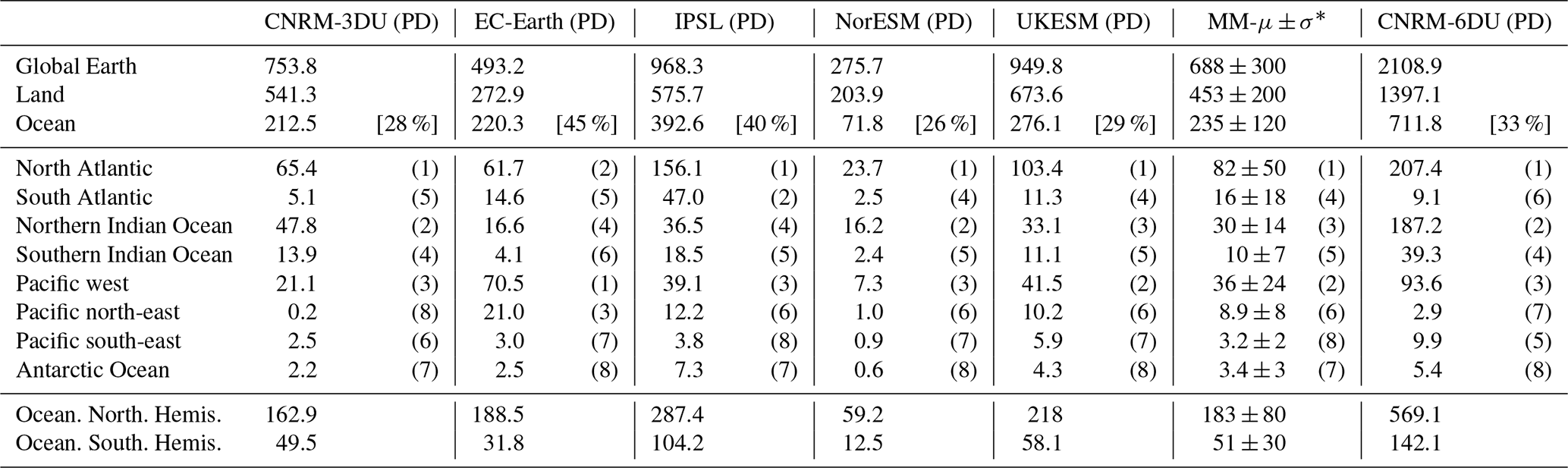
^* Statistic does not include CNRM-6DU.

Table 10 Total dry deposition [Tg yr⁻¹] for present-day (PD) simulations over oceanic regions; see Fig. 2. The numbers in brackets show the fraction of global deposition over the ocean. The numbers in parentheses indicate the ranking order of contributions to the global total dry deposition by region from the highest to the lowest. The ensemble mean (and standard deviation) includes all the models except CNRM-6DU and UKESM. The equivalent tables for the PI and PDN experiments are in the Supplement: Tables S.DD.3 and S.DD.4, respectively. The ensemble statistics for global Earth and land do not include UKESM due to their large values of gravitational settling that would drive the estimate over ocean regions.

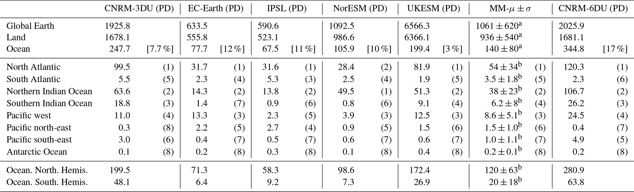
^a Statistic does not include CNRM-6DU and UKESM. ^b Statistic does not include CNRM-6DU.

Despite the different schemes all of them agree that the regions where most dust is uplifted are subtropical arid and semi-arid regions. Such regions are characterised by atmospheric stability and scarce rainfall. This global pattern is, however, modulated by Intertropical Convergence Zone (ITCZ) oscillations, monsoons and orography, as visible in Figs. 5 and 6. Because the Himalayan mountains filter the water vapour transport from the Indian Ocean all the models have important dust sources in northern Asia (such as the Taklamakan and Gobi deserts), but the specific location of Asian sources and their relative contribution to global emissions differ significantly between models.

Nowadays, we understand how regional climate influences dust emissions and their variability, together with the atmospheric systems linked to dust emission episodes. But dust emission modelling still constitutes an active research field (Shao, 2008). In particular, the dust particle size distribution (DPSD) at emission is critical for a better description of the global dust cycle (Mahowald et al., 2014), but its modelling needs to be improved for three main reasons: (1) because there is not a unified approach, (2) because there are discrepancies in the role of wind speed at emission for larger dust particles (Alfaro et al., 1998, 1997), and (3) because the quantitative link between soil properties and dust emission fluxes still needs additional research.

Regardless of the several sets of parameterisations of DPSD at emission (Kok, 2011; Alfaro and Gomes, 2001; Shao, 2001, 2004), the actual modelling of dust in global climate models is highly influenced by a balance of the different elements involved (vertical flux at small scale, soil erodibility, wind fields), which explains that during the last decade the estimation of dust emissions when online-coupled with meteorological fields has improved their results significantly. On the one hand, the modelled wind surface friction velocity and speed agree better with actual meteorological conditions; e.g. Knippertz and Stuut (2014). On the other hand, the description of the soil surface properties has become more accurate due to both improvements in soil texture databases and the use of satellite retrievals to better describe the roughness length; e.g. Prigent et al. (2005) and Menut et al. (2013).

All those facts explain why the comparison (Table 8) of the emissions (PD experiment) over large regions is fairly consistent among models: they agree on the main source of mineral dust being located in the Saharan desert but represent 39 % of total global emissions in the EC-Earth model and 66 % in CNRM-3DU. Previous studies (Shao et al., 2011) estimated the contribution of Africa to dust emissions in the range from 50 % to 68 % but also including Namibian desert emissions. The consistency is larger when we consider larger regions like hemispherical contributions, for which all the models show more than 85 % of global dust emissions from the Northern Hemisphere. When smaller regions are considered, the differences in relative contributions between models increase, which is also expected when turbulence at small scale and/or convection (Allen et al., 2015) play a role in dust events. If we evaluate total values rather than relative contributions, the driving factor that explains differences between modelled emissions is the upper threshold of particle sizes at emission.

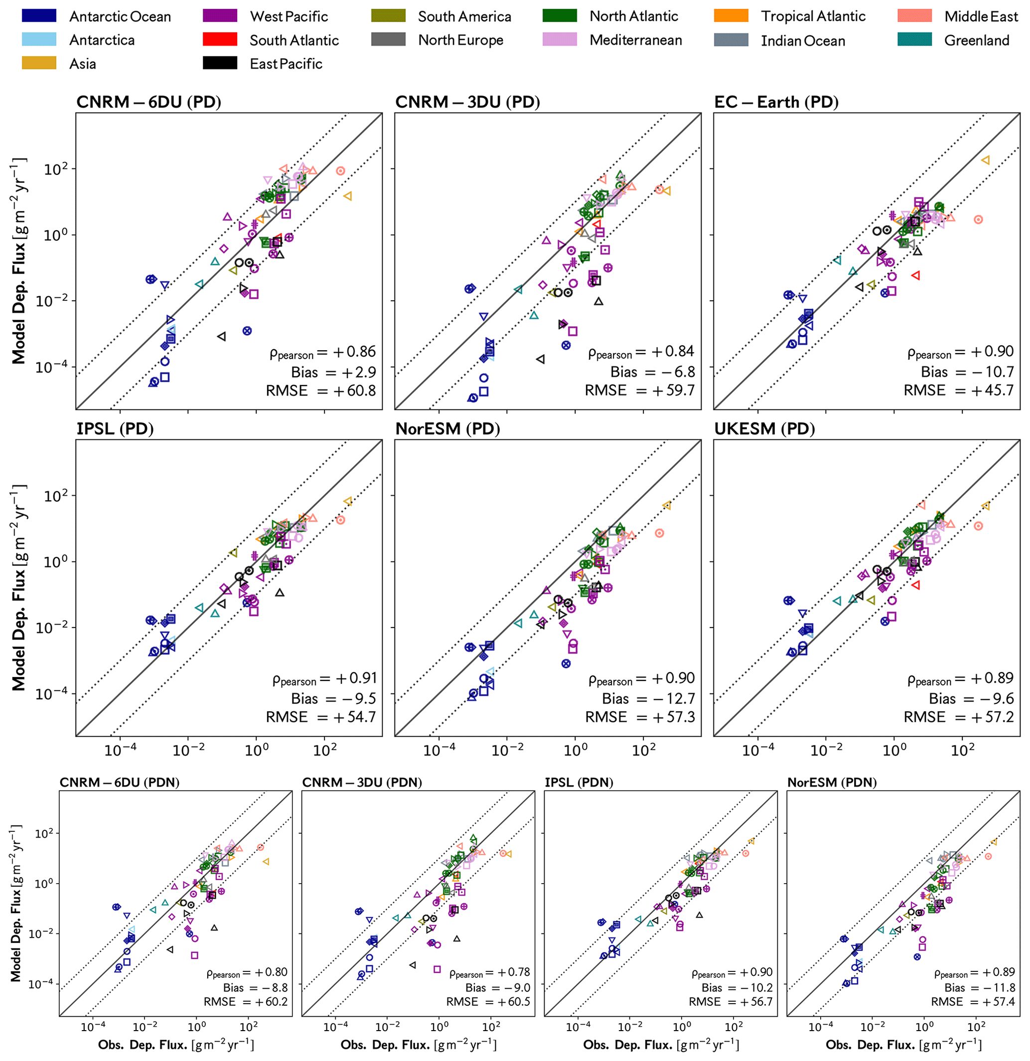
Figure 8 Comparison of estimated total annual deposition flux by CRESCENDO ESMs with the dataset presented by Huneeus et al. (2011), whose stations are mapped in Fig. 1 (left panel). The model values taken are those from the PD experiment (top part) and the PDN experiment for the bottom row. Figure S.D11 is the analogue of this figure but for the PI experiment.

Dust emissions by region (which are shown in Fig. 3) and their intensities (in Tg yr⁻¹) are listed in Table 8 for the PD experiment. The most intense source of dust for the EC-Earth model is located over the Gobi Desert, while the northern Sahara, a key emitting region in all other models, constitutes only the fourth most intense region in emissions (after the Taklamakan and the Kyzyl Kum). The Bodélé is a remarkably important dust source across all CRESCENDO ESMs. As expected from the analysis of dust optical depth over Asian regions, the Taklamakan, Kyzyl Kum and Thar deserts exhibit substantial differences. Regarding UKESM, it has an additional and extended dust source over the Somali desert (see Fig. 5), which is only a relatively small source in other models. Analogues of Table 8 for the PDN and the PI experiments can be found in Tables S.DE.1 to S.DE.4, respectively, showing similar model differences.

If we want to realistically compare global climate model emissions over smaller regions, we need to account for the different model resolutions. We opted to display normalised emission estimations over a common grid for all the models. Our method interpolates the emission flux from each model grid to that with the highest spatial resolution (NorESM). We use a near-neighbour interpolation method, which conserves the flux in each model when compared to the flux integrated over the original model resolution. This method does not introduce any ad hoc information on how the emission tendency is distributed within the original grid pixel. A monthly time series of normalised emitted dust mass per grid pixel, with respect to global monthly emissions, is produced using this method. These normalised emissions over a common grid allow us to pick up differences over locations that are caused either by the formulation of the source function or by the dust particle size distribution imposed during the emission process.

A direct comparison of dust emission maps with observations is challenging because it would require the translation of the observed frequency of dust events into a dust emission flux rate (Evan et al., 2015). Assuming the hypothesis of Evan et al. (2015) for this mapping, the hot spots of their Spinning Enhanced Visible and InfraRed Imager (SEVIRI) emission-normalised product can be compared with our normalised maps (in terms of the relative contribution of different pixels over North Africa). In particular, they suggest that beyond the Bodélé Depression an important source is in the Hoggar Mountains (west of Bodélé Depression). This feature is only captured by the CNRM models.

Figure 9 Comparison of estimated total annual deposition flux by CRESCENDO ESMs with the dataset stations shown in Fig. 1 (right panel). The model values taken are those from the PD experiment (top part) and PDN experiment for the bottom row. Figure S.D.11 in the Supplement is the analogous figure for the PI experiment. Vertical bars in the bottom panel represent the year-to-year internal variability captured by each model. The grey horizontal bars displayed for the Sahel stations represent the year-to-year variations in the observations.

The annual average of these monthly maps is presented in Fig. 7 for the PD and PDN experiments. The models CNRM-6DU and CNRM-3DU show similar values per grid cell, which indicates the use of the same information on soil properties, but the normalised emissions, although similar, are not identical, reflecting the differences in dust size distribution at emission. In these models, the normalised emissions over Australia are higher than for the other models, and this difference also appears in the optical depths simulated at the AERONET station of Birdsville. Their description of semi-desert areas in northern India has many similarities to the IPSL model. Emission tendencies from the UKESM extend to areas where other models do not simulate emissions, and the pattern of emissions is more smooth. In particular, significant emissions occur over the Sahel, Ethiopia, Somalia and India. For these regions, higher dust emissions in UKESM could have a stronger impact on African and Asian monsoons. The most granulated pattern is found for NorESM due to the higher resolution of the source functions implemented. The last row in Fig. 7 corresponds to the normalised emission maps for the PDN experiment, and it indicates that although there are important differences between the PD and PDN experiments in terms of total emissions (see Table 8), the spatial patterns of emissions are similar once they are normalised. We can ascertain this fact by comparing the CNRM-6DU normalised emission maps for the PD and the PDN experiment. The analysis for the PI experiment is in the Supplement: Fig. S.DE.5.

5.4 Dust deposition

Previous studies (Huneeus et al., 2011; Albani et al., 2014) show that total deposition of dust, when compared with in situ measurements, agrees globally only to within a factor of 10. Part of the reason is that dry deposition and wet deposition are dependent on the dust particle size distribution, whose representation is challenging for current global climate models. Indeed, processes driving dry deposition such as turbulent motions of particles and gravitational settling are both particle-size-dependent, as the aerodynamic resistance and the terminal velocity due to friction depend on the effective dust particle diameter. Wet deposition during precipitation events also depends on the size of the particle (Seinfeld and Pandis, 1998), but measurements of aerosol lifetimes below clouds are scarce. Furthermore, other aerosol processes inside clouds modify the aerosol size distribution, as well as their optical properties, essentially due to potential aggregation of water-coated aerosols (Mahowald et al., 2014). Thereby, the first step of the analysis is a comparison of dry and wet deposition at a regional scale.

Table 11 Statistical properties of the comparison of the CRESCENDO ESMs' total deposition against the Network-SET-M (see Fig. 1b). Statistical metrics used in this table are described in Table 5: Pearson correlation coefficient (ρ), bias (δ) [${\mathrm{gm}}^{-\mathrm{2}}{\mathrm{yr}}^{-\mathrm{1}}$], normalised bias (δ_N), ratio standard deviations (Σ), normalised mean absolute error (θ_N) and root mean square error (RMSE =η).

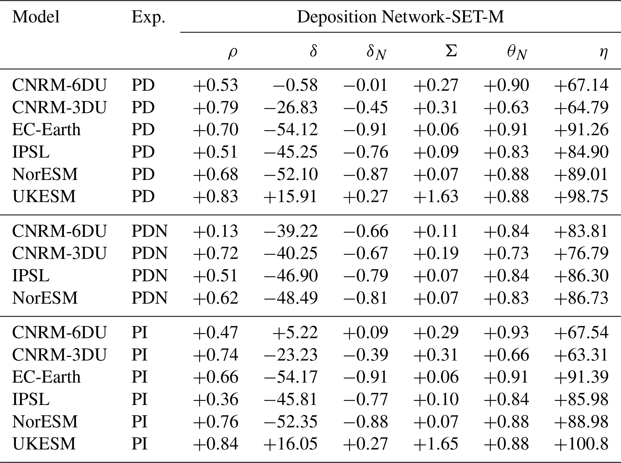
Table 12 Statistical properties of the comparison of the CRESCENDO ESMs' total deposition against the Network-H2011 (see Fig. 1a). Statistical metrics used in this table are described in Table 5: Pearson correlation coefficient (ρ), bias (δ) [$\mathrm{g}{\mathrm{m}}^{-\mathrm{2}}{\mathrm{yr}}^{-\mathrm{1}}$], normalised bias (δ_N), ratio standard deviations (Σ), normalised mean absolute error (θ_N) and root mean square error (RMSE =η).

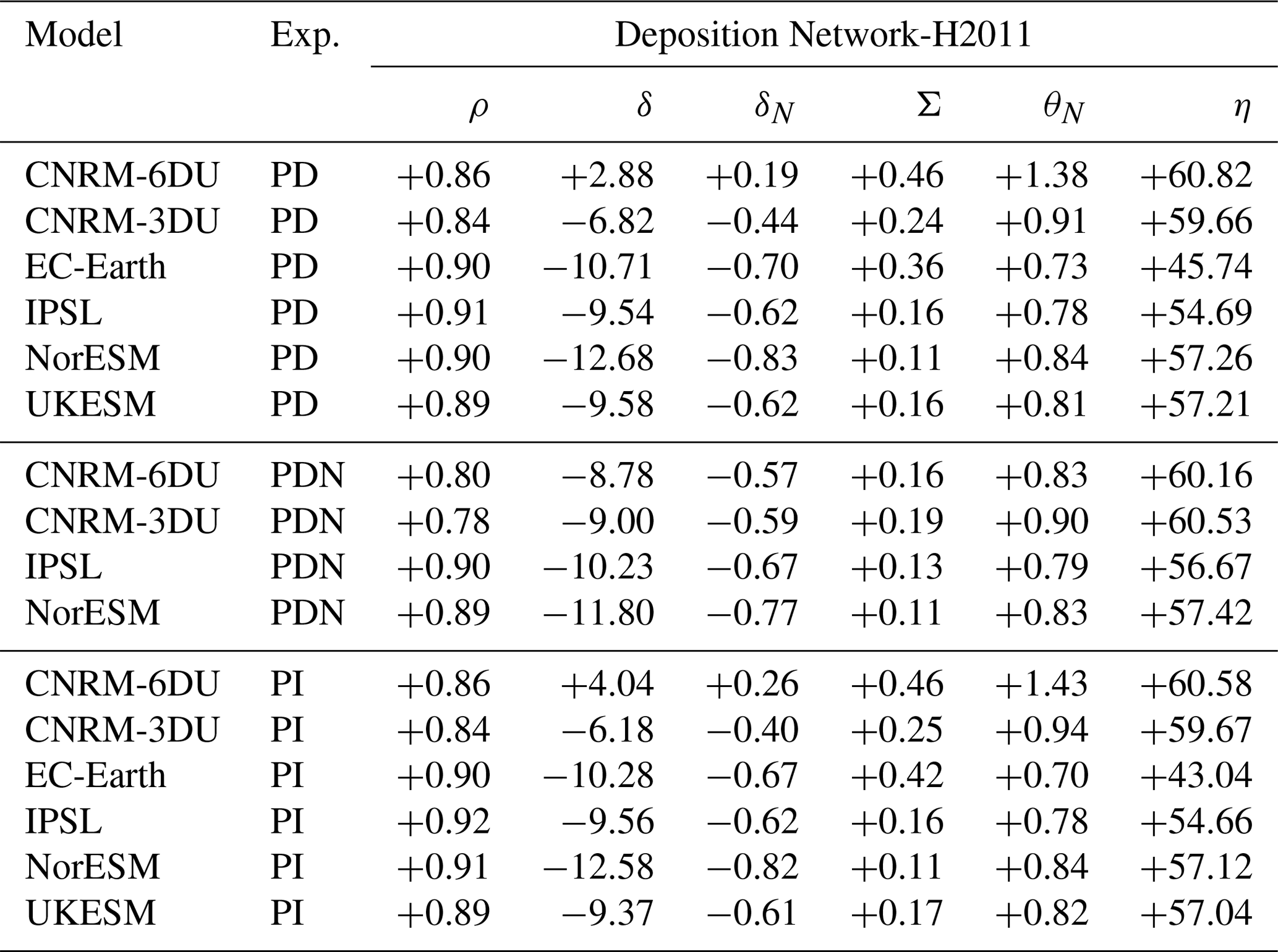
In fact, as the gravitational settling of large particles is dominant close to dust sources, regions remote from the main emission sources are well suited to compare models with different emission schemes and evaluate their respective total dry and wet deposition. Close to dust sources the upper threshold of the emitted dust particle sizes plays a role in the comparison with measurements. In particular, wet deposition over oceanic regions is enhanced relative to dry deposition, which motivates targeting these specific regions for comparison. Tables 9 and 10 show the regional analysis of wet and dry deposition (including the sedimentation–gravitational settling) over oceans. These results are globally consistent with those shown by Shao et al. (2011). The two main oceanic regions where dust deposition occurs are the North Atlantic and the Indian Ocean, even though the EC-Earth model simulated the largest dust wet deposition over the western Pacific Ocean. For all models, the fraction of dry and wet deposition over the oceans is smaller than over land. Wet deposition over oceans represents 40 % and 45 % of the total wet deposition for IPSL and EC-Earth, respectively. But for NorESM it represents 26 % of the global wet deposition. Dry deposition over oceans ranges from 3 % to 12 % of global dry deposition. For the UKESM, the dry deposition over land is 97 % of the total dry deposition due to the gravitational settling of large particles close to emission regions. Tables 9 and 10 also show slightly better consistency in the total dry deposition over oceans in the model ensemble (from 67 to 250 in Tg yr⁻¹) than in the wet deposition (72 to 392 in Tg yr⁻¹), as we exclude CNRM-6DU from the model ensemble. Results for the PDN and PI experiments are included in Tables S.DD.1 to S.DD.4.

5.4.1 Network of dust deposition observations

Figure 8 shows the total annual deposition for the PD and PDN experiments for the locations shown in panel (a) of Fig. 1, and Fig. 9 shows the total annual deposition for the PD and PDN experiments for the locations shown in panel (b) of Fig. 1. Figures S.DD.11 and S.DD.12 show the analogues for the PI experiment. Qualitatively the global results are similar to Huneeus et al. (2011), wherein at most of the stations the modelled deposition is within a factor of 10 of the observed deposition flux (in the figures, the region between the dotted lines). As a consequence the estimated Pearson correlation of deposition flux calculated over log values for the full network shows a reasonable value for all models.

Figure 10 Seasonal cycle relative to the annual mean value of dust optical depth as modelled by CRESCENDO ESMs over 15 regions. These seasonal cycles are compared against the DOD product of derived dust optical depth over land based on MODIS deep-blue retrievals (Pu and Ginoux, 2018b); see the Supplement for a description of how these products are derived and the analogous figure for the PDN and PI experiments.

All the models agree that Antarctica and the Southern Ocean have the lowest values of total deposition. While UKESM and IPSL tend to slightly overestimate the total flux in these remote regions, the CNRM models tend to underestimate the flux. However, their most prominent property in Antarctic regions is a much larger range of values than the range reported by the observations. Additional research is needed to evaluate if this is a consequence of their semi-Lagrangian model implemented in their dynamical core, which adds a non-uniform bias, or is instead just a combination of the dust source locations in the Southern Hemisphere and wind fields modelled.

Regarding the Pacific region closer to North America (eastern Pacific), NorESM, CNRM-6DU and CNRM-3DU tend to underestimate the deposition. In the case of the western Pacific region NorESM systematically underestimates the deposition flux. The CNRM models underestimate the total deposition over the Northern Hemisphere part of the western Pacific but not in the southern part of the western Pacific, probably due to the enhanced emissions of these models over Australian deserts. All the models except the EC-Earth model underestimate the deposition over the single Asia station, and the EC-Earth model reports good values of total deposition over the northern part of the western Pacific as it has the largest relative contributions over the Gobi Desert between all the models.

All the models show good agreement in the Atlantic region (both the north and tropical regions) and the Middle East, although the UKESM and EC-Earth models underestimate the values at the single station in the South Atlantic. The deposition fluxes over the Indian Ocean are fairly well described by all models.

If we compare the observations against the modelled total deposition obtained from the experiment with nudged winds (last row in Fig. 8), the correlation coefficients are similar, but differences between models are reduced, especially for the CNRM models. This is illustrated in Table 12 with a negative bias for all models (from −8.8 to −11.8 $\mathrm{g}{\mathrm{m}}^{-\mathrm{2}}{\mathrm{yr}}^{-\mathrm{1}}$), and the ratio of standard deviations (Σ) ranges between 0.11 and 0.19 (for PD experiment between 0.11 and 0.46). The CNRM-6DU model is the only one with a positive bias (δ in Table 12) against the Network-H2011.

Figure 11 Skill of CRESCENDO ESMs by region calculated as the Pearson correlations between the ESM time series of dust optical depth for each season and that from MODIS DOD. The time interval spans 2001 to 2014. It assesses the performance of the different models in reproducing the inter-annual variability of each season against observations over dust source regions.

In Fig. 9 we analyse the ability of the ESMs to reproduce deposition fluxes regionally and closer to sources (for the PD and PDN experiments). We focus on the Mediterranean Sea, but we include three additional stations over the Sahel where observational annual differences can be compared. The analysis reveals that only the UKESM reproduces the full range of observed deposition fluxes. All the other models underestimate total deposition fluxes over stations where fluxes exceed 100 $\mathrm{g}{\mathrm{m}}^{-\mathrm{2}}{\mathrm{yr}}^{-\mathrm{1}}$, and only the CNRM-3DU model estimates the observed dust deposition well in the northern Mediterranean Sea. Over the Sahel region, the CNRM models and UKESM provide reasonable values of total deposition flux, but UKESM overestimates the inland deposition, whereas the other models show a more consistent bias over the whole region.

The Sahel stations include horizontal bars describing the inter-annual variability over the mean values, which can be compared with vertical bars describing the variability in the models. In this case EC-Earth is the model that best captures the year-to-year differences in mean values of dust deposition flux over the inland Sahel stations. For the western Mediterranean the CNRM-3DU has the smallest bias, whereas in the full Mediterranean region UKESM and IPSL perform well in terms of global bias.

EC-Earth and NorESM underestimate total deposition close to source regions, consistent with the applied size cutoff of around 8 µm of emitted particles, and CNRM-6DU overestimates the deposition in the whole Mediterranean region. For the experiment with nudged winds, we observe better consistency between models, with all of them showing similar values of total deposition in the different subregions. However, this implies an underestimation over the Sahel for the CNRM-6DU model, which also has the largest inter-annual variability over the western Mediterranean. The statistical metrics are shown in Table 11.

Figure 12 Normalised Taylor diagrams based on time series of total aerosol optical depths at 440 nm. These diagrams represent the PD and PDN experiments and are restricted to AERONET dusty stations shown in Fig. 3 (with the colours green and blue).

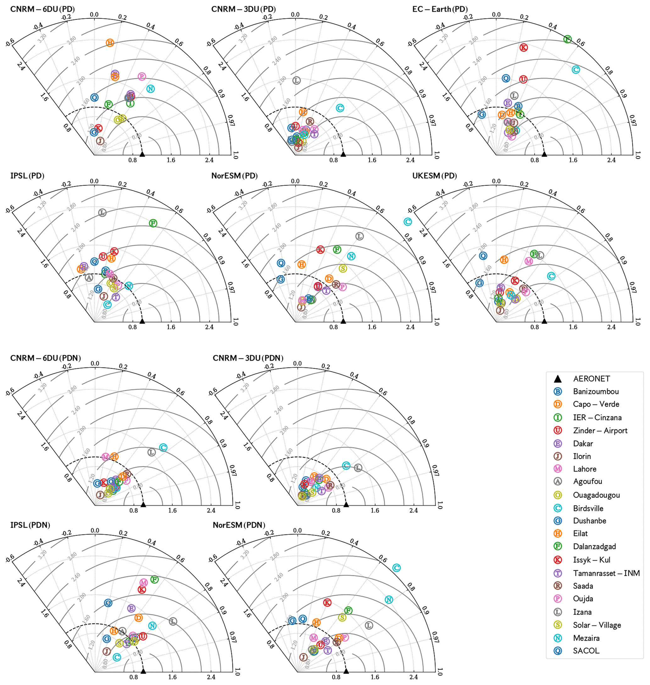
5.5 Dust optical depth

The simulated dust optical depth (DOD) by climate models has been previously compared with those retrieved through a network of ground-based sun photometers (Huneeus et al., 2011) but also with products derived from satellite retrievals (Pu and Ginoux, 2018b; Peyridieu et al., 2013). There are also intercomparisons between global climate models (Shindell et al., 2013). The overall agreement reported by these studies between retrieved and simulated dust aerosol optical depth is within a factor of 2. Those results support the reliability of global estimations of the radiative effect from mineral dust. However, given that it is a vertically integrated parameter, it masks larger differences present in partial column estimates.

Our study focuses first on the comparison in regions defined in Fig. 3. We compare the DOD of the CRESCENDO ESMs with satellites and intercompare simulated dust optical depth. Figure 10 shows the seasonal cycle (relative to the annual mean value of each model) and the MODIS DOD product during the period 2001–2014 for the PD experiment (the PDN and PI experiments are shown in Figs. S.DOD.1 and S.DOD.2). We can hence analyse the seasonal amplitude relative to the annual background signal per region for each model. The Supplement Fig. S.DOD.3 shows the direct comparison of the seasonal cycle without relative values.

Over the most prominent preferential dust source regions (first row of Fig. 10), the amplitude of the seasonal variability is systematically larger in all the models (with respect to the MODIS DOD product), with a slight offset in the maximum value of the seasonal cycle towards springtime, particularly over the northern Sahara. It is remarkable that in these regions CNRM-3DU and NorESM show consistency in the seasonality with respect to MODIS DOD, whereas EC-Earth and UKESM show more discrepancies in the seasonal cycle in both the amplitude and the phase. The CNRM-6DU model and IPSL have slight discrepancies in these four regions. Over the Asian deserts (the Taklamakan and Gobi) the seasonal maximum is reasonably represented in the spring with relatively good agreement for EC-Earth, although the seasonality is not well represented for the Thar Desert. The UKESM, NorESM and CNRM-3DU models overestimate summer dust optical depth over the Taklamakan desert. A common feature between all the models is that over the Asian desert the winter values are smaller than those of MODIS DOD. Previous studies (Laurent et al., 2006) concluded that the seasonal cycle of the Taklamakan desert is controlled by later spring and summer emissions, which most models capture, whereas the Gobi and the associated northern China deserts have maximum emissions during late winter and early spring. CRESCENDO ESMs reproduce the maximum values of DOD in spring for the Gobi Desert, and UKESM and EC-Earth capture that seasonality over the Taklamakan as well. Given the structural differences in the soil properties of these Asian regions (more stony at the Gobi, mostly sandy at Taklamakan) and the additional role of snow cover over the Gobi Desert, further model studies of Asian dust emissions are needed to better constrain the way dust scheme parameterisations capture emissions in these regions. Ideally, these studies should be backed up by in situ surface concentration measurements. Regarding the Middle East, the combined region of the northern and southern Middle East is in agreement with the Pu and Ginoux (2018b) study based on CMIP5 models.

We quantified the performance skill of the CRESCENDO ESMs by estimating the Pearson's correlation between the time series of dust optical depth provided by each model for each of the seasons and the same time series of dates given by the MODIS DOD product for the period between January 2001 and December 2014.

Figure 11 displays the values for this Pearson's correlation. The overall assessment indicates marked differences between models for the same season and over the same region. In the case of the PD experiment (middle panel), the correlation between MODIS DOD and CRESCENDO ESMs is positive over winter except in the Australia and southern Africa regions, which are regions particularly challenging for the ESMs analysed as we reported negative correlations, whereas South America is one of the regions with a correlation closer to zero across all the seasons (and models). The overall correlation decreases in spring (with respect to winter), as we notice multiple regions where the Pearson correlations are close to zero. In summer, except in the Gulf of Guinea, the correlation is also smaller than in the winter season. Finally, in autumn the performance over the Middle East and the Kyzyl Kum region is improved. The better behaviour of all the models is given over the Bodélé in the winter season and the Arabian region (northern and southern Middle East), which shows reasonable agreement all year for almost all models. Most of the features remain similar with pre-industrial aerosol–chemistry forcings (PI experiment), and the CNRM-6DU and CNMR-3DU behave identically in the PI experiment.

The agreement with satellite platforms is significantly improved for the PDN simulations, and the consistency between models is enhanced. In particular, the Saharan region shows a marked improvement in the simulated dust optical depth. Australia and southern Africa are still the regions where most discrepancies are found, and South America systematically has the correlation closest to zero.

We extended the analysis based on the Pearson correlation by using the Spearman coefficient, which allows detecting non-linear correlations. The results for the Spearman rank coefficient can be found in the Supplement in Fig. S.DOD.7; they yield similar conclusions, and both methods are consistent.

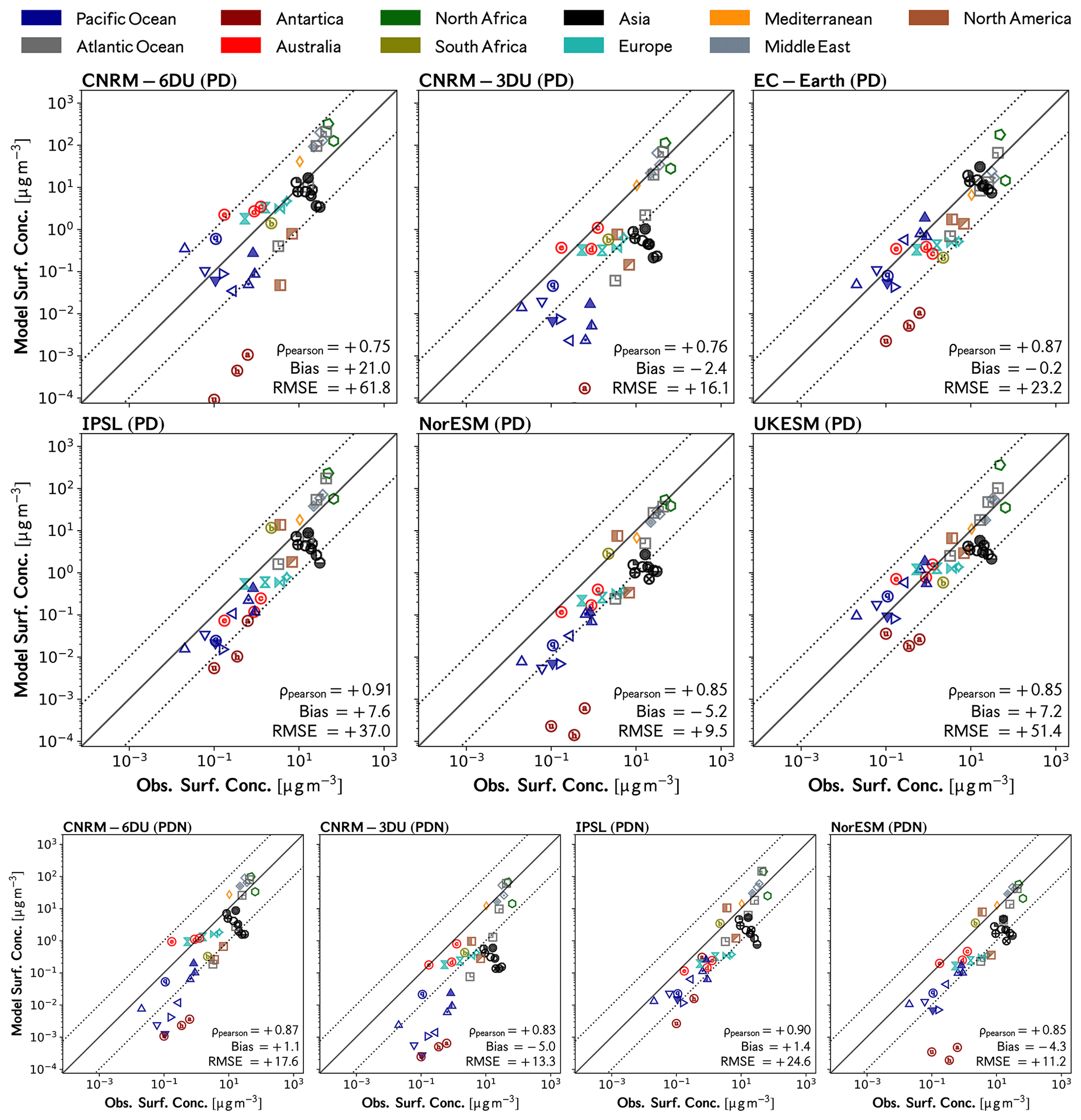
Figure 13 Comparison of dust surface concentrations in the models with the climatological dataset of Prospero and Nees (1986) and Prospero and Savoie (1989) for the PD and PDN experiments. The colours of the points indicate the region to which the measurement station belongs. Climatological datasets were obtained from observations over the period from 1991 to 1994. For the PI experiment see Fig. S.SDC.10.

5.5.1 Network of aerosol optical depth

The comparison relies on the dominantly dusty AERONET stations described in Sect. 3.4. For each station the monthly time series of total aerosol optical depth at 440 nm are compared with the climate model value at the grid cell wherein the station is located. As we are considering dusty stations, the correlation of the time series represents how well the seasonal cycle is captured or not, while the representation of the amplitude of the cycle is measured by the standard deviation. Therefore, the ratio of standard deviations is an indication of the agreement in seasonal amplitude between the models and observations. Those statistics are compared using a normalised Taylor diagram (Taylor, 2001). These diagrams are shown in Fig. 12 for the PD and PDN simulations. The behaviour of each model with respect to the observations at a station is indicated by both its radial and angle values: the radial value indicates the normalised standard deviation with respect to observations, and the angle measures the correlation between time series.

Table 13 Statistical properties of the comparison of the CRESCENDO ESMs' dust surface concentration with respect to the global network shown in Fig. 2. Statistical metrics used in this table are described in Table 5: Pearson correlation coefficient (ρ), bias (δ) [µg m⁻³], normalised bias (δ_N), ratio standard deviations (Σ), normalised mean absolute error (θ_N) and root mean square error (RMSE =η).

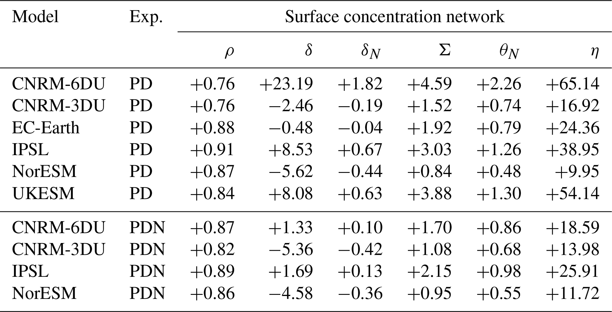
A common result across all models comparing the PD and PDN experiments is the higher correlation for simulations with nudged winds but a similar normalised standard deviation for the cloud of points. With nudged winds the correlation is always positive except at one station for NorESM, a model that has a correlation larger than 0.6 for 13 stations in PDN (nine stations for PD). The PD experiment has only one case with correlation values around 0.8 (NorESM at Oujda), but all the models in the PDN experiment have stations with correlations larger than 0.8, indicating that the seasonal cycle of optical depth is clearly improved with wind fields from reanalysis. The CNRM-6DU model has a strong change in the normalised standard deviation from PD (for which most of the stations have values larger than 1) to PDN (with most of the stations with values smaller than 1). In terms of the amplitude of the seasonal cycle, the most challenging stations for all models are in Australia (Birdsville station), the Gobi Desert (Dalanzadgad and Sacol) and Izaña (close to the Sahara but on an island and at high elevation). In terms of correlation, Dushanbe in the Thar region and Sacol (China) are challenging. On the other hand, stations like Sadaa (western Sahara), Eilat (northern Middle East) and Dakar are reasonably well captured by models.

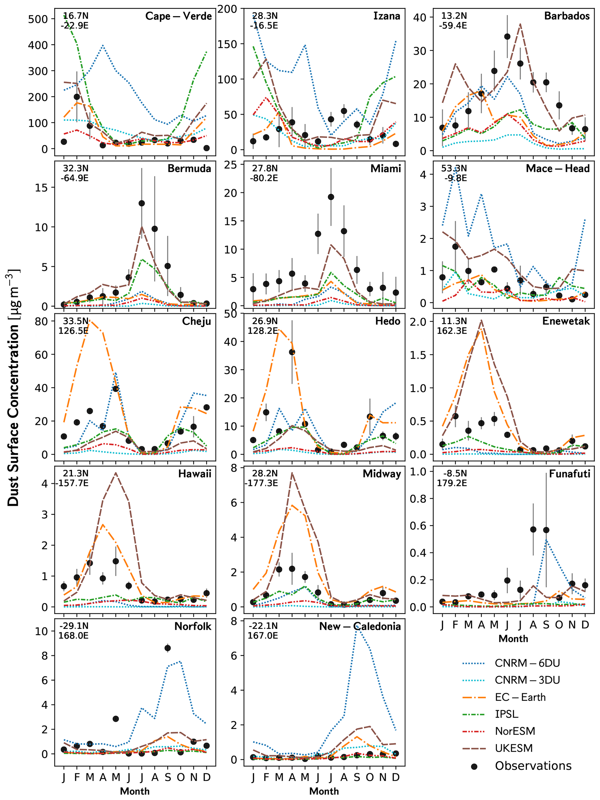
Figure 14 Comparison of ESM (PD) dust surface concentrations with a station-based climatological dataset. For the PI and PDN experiment see the Supplement Figs. S.DSC.7 and S.DSC.8.

5.6 Surface concentrations

The stations were chosen to cover a range of dust values from low to moderate dust concentrations, mainly located at a distance from the main dust emission regions. According to the instrument location, the Sahel and the west coast of North Africa (green and grey squares), together with the Middle East stations (grey diamonds), report the highest values of surface concentrations; see Fig. 13. The group represented by black circles shows moderate values, indicating transport of dust from arid and semi-arid regions of East Asia. The lowest values correspond to Antarctica and the Pacific Ocean (blue triangles). The values of the dataset are shown in Table S.MD.4 of the Supplement.

The comparison between the CRESCENDO models and a network of stations that measure dust surface concentrations is shown in Fig. 13 for the PD and PDN experiment and in Fig. S.DSC.10 for the PI experiment. The agreement falls into the same range as previous comparisons with the Community Atmospheric Model (CAM) (Albani et al., 2014) wherein the full range for the expected differences in annual mean values is close to 10. This range of differences between models compares well with the previous study from Huneeus et al. (2011).

CNRM-3DU underestimates dust concentrations over the Pacific Ocean. This behaviour over regions remote from dust sources could be partly due to the non-conservative semi-Lagrangian transport scheme that accentuates the differences with the distance of transport (a fact also consistent with their values of the Pearson correlation, mainly in nudged simulations). All models except IPSL underestimate the concentrations at the Antarctica station. This could be due to the larger emissions from Patagonia that cause an increase in the correlation coefficient for this model. Over northern Europe, all models except CNRM tend to underestimate dust concentrations and do not reproduce the range of variability found in the observations. When comparing PD and PDN simulations, IPSL and NorESM show slightly better agreement in PDN conditions, whereas the two CNRM models show higher correlations when using nudged winds but similar differences over the Pacific Ocean.

The correlation between the models and observations is significant for all models. The RMSE values are influenced by the stations with the highest concentrations and are hence more representative of the concentrations near the Sahara and the Middle East. In this regard, the NorESM and CNRM-3DU models show the best agreement over these regions. The EC-Earth model, however, shows the smallest bias because it better captures dust concentrations over Japan and eastern China, where the other models underestimate concentrations. Values of normalised bias and normalised mean absolute error complement the previous metrics and give us a characterisation of global differences equally accounting for the stations with the lowest concentrations (see Table 13). The normalised statistics indicate that the nudged wind simulations generally show better agreement with observations.

Although the 36 stations cover many regions, a complete assessment of the model performance at the surface is not possible due to the absence of stations in South America and Asia and the presence of only one station inland over North America and Africa. Therefore, the global observational constraints, in terms of the surface concentrations, are only partial.

The comparison of the seasonal cycle of surface concentrations against 14 stations is shown in Fig. 14 for the PD experiment. The stations Cape Verde and Barbados are at the same latitude on opposite sides of the Atlantic; therefore, they have a signature of the trans-Atlantic transport of mineral dust from the Sahel region. The IPSL, CNRM-6DU and UKESM overestimate the early winter contributions to the seasonal cycle in Cape Verde. The models reproduce the concentrations within a factor of 2 from May to September (except CNRM-6DU model) with a general overestimation except for EC-Earth. However, in the case of Barbados, UKESM after April and CNRM-6DU before May reproduce the surface concentrations very well. All the other models, although with a similar seasonal cycle, underestimate the total surface concentrations by a factor of 2 to 4. The stations Izaña, Bermuda and Miami also have similar latitudes and represent the Atlantic transport from the western Sahara. Izaña Observatory is not at sea level, and all the models have difficulties reproducing the seasonal cycle. The seasonal cycles of Bermuda and Miami are well reproduced, with a general underestimation of the surface concentrations values; only UKESM and IPSL show consistency within a factor of 2. Cheju and Hedo are stations on the western Pacific coast, and their measurements represent the dust transport from China. The EC-Earth model reproduces the seasonal cycle well but with an overestimation of spring concentrations by a factor of 3. The seasonal cycle and values are well represented by the CNRM-6DU and IPSL models. Enewetak is located between the Philippines and Hawaii in the middle of the Pacific Ocean, and EC-Earth and UKESM overestimate the spring concentrations, whereas all the other models underestimate them. A similar situation is found in Hawaii and Midway. The rest of the stations are in the Southern Hemisphere where the dust concentrations are smaller and the seasonal cycle is only partially reproduced. The results for the PDN experiment (see the Supplement DSC) are similar with a slight improvement in the seasonal cycle but with a general underestimation of surface concentrations. All the models with nudged winds exhibit problems in reproducing the observations in Izaña.

6 Discussion and conclusions

The analysis of the results provides insight into how the combination of modelling and measurements of dust can be used to improve our understanding of the dust cycle.

A first approach to the evaluation of the dust cycle relies on in the total dust loads and emissions. In this regard, we have shown that the model ensemble values of total emissions with nudged winds have less dispersion. We stress, however, that dust column loads are a better quantity when comparing models with different size distributions at emission than comparing total emission fluxes, since gravitational settling gets rid of the very large particles over a short time span. For dust loads, all models in PDN experiments are in a range between 9.1 and 15.2 Tg, which can serve as a baseline to study model improvements. Because new studies support the important role of the coarse mode of dust (Huang et al., 2020), it is recommended to compare the contributions to dust load for the fine and coarse modes separately. The range of dust loadings that we obtained is smaller than recent estimations (Kok et al., 2021b) that propose values ≳ 20 Tg with a multi-model comparison to models with geometric diameters up to 20 µm but based on a new methodology whereby the dust diagnostics include observational constraints (Kok et al., 2021a). Actually, Adebiyi and Kok (2020) propose that the total load of dust in the atmosphere is higher than what is typically estimated and give a mean value close to 30 Tg, to which the contribution of the coarse mode is more important than the fine mode.

Therefore, annual global dust emissions from climate models are dependent on the dust particle size distribution (DPSD) representation. The first result we observe is that models that account for particles with diameters larger than 10 µm produce higher total fluxes. However, although an important diversity in the total emissions depends on the upper threshold, specific boundaries of the bin for the largest particles used in a sectional scheme also seem critical. We observed large differences in total emissions between UKESM1 and CNRM-6DU for which an important difference is the lower boundary of the last bin diameter: 20 and 10 µm, respectively. For this reason we have proposed two classifiers for further model analysis, but we still need a reasonable metric to compare the emissions at grid cell scale.

To overcome the challenge of comparing models with different DPSDs at emission, we introduced normalised emission maps, showing first (through a comparison between the PD and PDN simulations) that wind fields do not substantially affect these normalised emission estimates in terms of spatial patterns when we analyse the 15-year emission means of the PD and PDN simulations. This led us to interpret differences in regions where dust was emitted as reflecting differences in the underlying dust effective soil erodibility information (DESEI) among models. However, the DESEI also includes a sort of meteorological factor because of the role of soil moisture in the emission process, together with specific properties of the dust scheme like the threshold in friction velocity and how the soil texture is translated into a dust size distribution. Note that the simulations compared in our study share the same sea surface temperatures, which reduces the model diversity in terms of precipitation. Nonetheless, the consistency we report between the PD and PDN normalised emission maps needs further investigation at smaller spatial and temporal scales, in particular at daily and sub-daily scales.

Beyond the interpretation of the re-gridded normalised emission maps, they allow us to compare the relative intensity contribution to dust emissions on the same spatial scale. It is a useful tool, as a direct balance of the several source functions is complex. For example, with the aim of reproducing dust observations at different model resolutions, models have introduced correction factors to their dust soil erodibility (see, for example, Albani et al., 2014 and Knippertz and Todd, 2012). In contrast, our normalised emissions can indicate effective model differences in both intensity and location for preferential dust sources. We found that these differences are the largest over Asia and are also significant over Australia. Hence, we identified these regions as two source regions that would benefit from further comparison of dust emission observations with actual model occurrences in emission fluxes. Moreover, the diversity in Asian emissions is investigated by Kok et al. (2021b), also obtaining important differences with AeroCom Phase I models and suggesting an underestimation of dust emission from East Asian deserts. Finally, additional research is also needed to ascertain seasonality disagreements in dust sources, which our 15-year mean normalised emission maps do not show but for which seasonally normalised emission maps would be a useful tool.

Regarding dust deposition, another important point of discrepancy between models is the ratio between wet and dry deposition over similar particle size ranges, indicating that specific sensitivity studies should focus on the treatment of deposition. Interestingly, we have found that there is not a correlation between the modelling of the largest particles and the value of this ratio. Finally, evidence of significant differences is also found in deposition over the oceans, in particular over the Indian Ocean and over the Pacific west, both of which are affected by dust source distributions over Asia.

To properly evaluate the impact of dust on the climate system, it is important to determine an uncertainty range of the direct radiative effects for each model. Based on a calculation with four modes over a range from 0.1 to 100 µm, we observe that models without the smallest particles (without mode m₁) will underestimate the shortwave contribution at the TOA by up to 20 %. Models without the largest particles (those represented by the m₂₂, i.e. for bins with a diameter larger than 40 µm), however, are not expected to be significantly affected in their estimations of DRE in the SW. Nevertheless, we need additional studies to determine whether these estimates are consistent with other models with the same range of modelled dust size particles. In particular, it is recommended to attribute diversity in the context of the several refractive indices.

The dust optical depth is a key diagnostic in comparative studies. It appears to be logical to try to constrain the dust cycle by relying on dust optical depth (DOD) estimated from satellite observations. This is because dust emissions depend on mineralogy, land surface properties and regional meteorology. Therefore, a few in situ measurements are not sufficient to constrain the dust cycle at any possible scale. Indeed, Ridley et al. (2016) used retrievals from instruments on board MODIS and MISR to estimate global values for DOD between 0.020 and 0.035, which place two models (CNRM-3DU and UKESM) outside this observational range. Note, however, that there are difficulties estimating DOD from satellite retrievals with the method of Ridley et al. (2016) because it still relies on model simulations to ascertain the fraction of non-dust optical depth. As shown by our results in the Supplement (Sect. DOD), the non-dust fraction of optical depth can have large inter-model differences. Furthermore, an important result is that, although DOD should be proportional to the mineral dust total column, the models with the lowest dust loadings are not those with the smallest DOD. This is illustrated in the differences in mass extinction efficiency (MEE) between the different models. The magnitude of MEE is a good indicator of intrinsic model properties due to its relatively small seasonal cycle, an aspect in which all the CRESCENDO ESMs match. But also, because mass extinction efficiency is affected by the DPSD and optical properties of mineral dust modelled, it is also a useful property to compare with observations.

Our analysis of dust optical depth includes a study at the regional scale. Specifically, the regional dust optical depth over dust source regions relies on a comparison with MODIS satellite estimates of DOD based on the algorithm described in Pu and Ginoux (2018b). This comparison allowed us to evaluate the skill of each model by evaluating the correlation between the regional time series of observations versus each model. A significant increase in the skill was revealed for the simulations using nudged winds, indicating that a consistent reproduction of the seasonal cycle depends critically on how strong surface winds are represented (with a improvement with the use of reanalysis wind datasets). However, the correlation (skill) is not useful in determining differences in the scale of the signal, and Fig. S.DOD.3 shows that there are regions where the seasonal cycle is well reproduced but the mean annual signal is actually underestimated; see also Pu and Ginoux (2018b). A further example of the difficulties in specific regions is given in the newly incorporated stations over Asia compared with Huneeus et al. (2011) because these stations have proven to be challenging for the CRESCENDO ESMs in terms of the comparison provided by Taylor diagrams (see Fig. 12).

7 Future research directions

Currently, the dust source disagreements and differences between models make it difficult to quantify the fraction of the uncertainties in dust emissions due to small-scale atmospheric phenomena that are not well represented by global models. The use of wind fields from reanalysis datasets reduces the differences between models, but a benchmark reference dataset regarding dust sources is needed to establish a range for those uncertainties. In particular, specific model comparisons based on common soil erodibility information would illuminate specific model improvements to decrease diversity. Indeed, these studies should use a similar prescribed seasonal vegetation fraction and bare soil distribution to improve the seasonal consistency.

The dust particle size distribution is a key point of research for current ESMs. Specifically, the global description of the dust cycle in terms of the amount of aerosol mass mobilised needs to be extended to larger particles as they can significantly increase the total emissions. At the same time, according to recent studies, the fraction of dust mass in the atmosphere due to coarser particles could be dominant with respect to the fine mode (Adebiyi and Kok, 2020). A further complication we found in our analysis is that the method by which the largest particles are incorporated in the models can drive strong differences in total emissions with ranges from 3500 Tg yr⁻¹ in CNRM-6DU to about 7000 Tg yr⁻¹ in the UKESM. In particular, the specific bins used to model the contribution of the largest particles are critical to understand model diversity. Additionally, a better discrimination of particles larger than 10µm but smaller than about 20 to 30 µm will occur if the results in the Table 7 are consistent between different models. This also illustrates that comparisons for which the particle size distribution is resolved (comparisons based on the contributions of each DPSD bin) are needed to better understand the source of model discrepancies; in that regard CRESCENDO ESM simulations were designed with these future evaluations in mind. Also, we created specific tools to estimate binned contributions from models based on modal DPSD (Checa-Garcia, 2020a) to support these comparisons.

However, these differences in total emissions are not directly translated into proportional loadings because of the differences in deposition between models and therefore in the lifetime. In particular, regarding total deposition one priority should be given to analysing the large differences in the ratio between dry and wet deposition between models, which is only partially explained by the modelled size distribution. From the aerosol microphysical point of view differences in the dominance of wet scavenging over ocean regions could account for some of these differences. However, as indicated by Shao et al. (2011), observations of dry deposition velocities in wind tunnels are not reproduced by current dry deposition schemes. In this scenario it becomes necessary to compare with measurements of wet and dry deposition separately (Marticorena et al., 2017). In fact, although our ensemble mean global contributions of gravitational settling, wet deposition and dry deposition without sedimentation are similar, there is large model diversity. To explain better the model diversity in sedimentation a first step is to ensure that gravitational settling is estimated for all atmospheric levels before a comparison of sedimentation for each size range. Because wet deposition involves modelling dust–cloud and dust–rainfall interactions the model diversity is partially conditioned by other parts of climate models (Croft et al., 2010). However, sensitivity studies for each model based on the plausible range of values of their dust scavenging coefficients (in-cloud and below-cloud) can provide valuable information on the actual range of uncertainties expected for each model.

The models exhibit important differences in preferential dust sources; in particular, better agreement of preferential sources found over Asia and Australia would give us more consistency in global dust transport over the Indian and Pacific oceans. Although there is a scarcity of measurement campaigns over Asia compared to the Sahara and Sahel, studies based on empirical relationships between visibility and dust surface concentrations give us an additional insight into dust sources over these regions (Shao and Dong, 2006). This information, supported by new regional studies, is needed to suggest the best lines of model improvements in these regions.

Given that the optical depth depends on column load rather than dust emission fluxes, inter-model convergence can be reasonably achieved even for models that do not implement particles with a radius larger than 10 µm. Also, inter-model convergence in terms of optical depth is important to better constrain the dust radiative forcings and direct radiative effects (DREs). However, as said earlier, the link between dust loads and dust optical depth, i.e. the MEE, shows important model differences. Additional MEE observations to better constrain the expected values would definitively help modellers to improve the dust load description by comparing with satellite dust optical depth estimates. Finally, given the different role of each mode (fine, coarse, super-coarse and giant) in the dust–radiation interaction, further studies, not only on the mineral composition but also on the possible dependence of the composition with size of dust particles, would improve our estimates of dust radiative forcings and direct radiative effects.

Appendix A: Method to estimate direct radiative effects in multi-modal size distributions

In Sect. 5.1 the direct radiative effects for a dust scheme with several dust modes were shown. Here we present the methods used to obtain the results in Table 7. The direct radiative effect of a species is defined by the Earth's instantaneous imbalance at the top of the atmosphere due to that specific atmospheric species or component. It has been introduced in Boucher and Tanré (2000) and discussed by Bellouin et al. (2013) and Heald et al. (2014). This imbalance is conceptually different from the radiative forcing (either defined as a stratospherically adjusted instantaneous radiative forcing or by an effective radiative forcing), which is a comparison between two different time periods, usually between pre-industrial times and the present day. In our case the direct radiative effects are estimated during a single simulation with present-day conditions but with multiple calls to the radiative transfer model implemented in the climate model. The aerosols in the climate model actually have direct, indirect and semi-direct effects in the simulation, but the method only estimated the direct radiative effects due to scattering and absorption of specific aerosol species. Therefore, there are observationally based estimations of the direct radiative effects of the aerosols (Yu et al., 2006). However, from the point of view of aerosol modelling based on multi-modal approaches, differences have been reported (Di Biagio et al., 2020) between (a) the calculation by the sum of each mode contribution estimated individually and (b) the estimation for the joint multi-modal directly.

In this Appendix two different approaches and a joint new method with four calls to the radiative scheme are described to decrease these differences.

In general, in the calculation done by current radiative transfer schemes it is considered a state of the atmosphere with several aerosols species represented by 𝒳 and 𝒴, for example, with each species possibly described by a multi-modal distribution with modes X₁, …, X_n. The state with all the aerosol species is hereafter named 𝒜 (therefore, $\mathcal{A}=\mathcal{X}\cup \mathcal{Y}\cup \mathcal{Z}\cup \mathrm{\dots }$). We define another state named $\stackrel{\mathrm{̃}}{\mathcal{A}}$ that includes all the modes of every aerosol species except those modes corresponding to the species 𝒳. Therefore, $\mathcal{A}=\stackrel{\mathrm{̃}}{\mathcal{A}}\cup \mathcal{X}$. The radiative effect of the aerosol 𝒳 described by several modes X₁, …, X_n is defined by

$$\widehat{{\mathcal{F}}_X}=\mathcal{R}(\mathcal{A},\mathit{\delta })-\mathcal{R}(\stackrel{\mathrm{̃}}{\mathcal{A}},\mathit{\delta }),$$

where ℛ represents the radiance obtained in our radiative transfer scheme, which is intrinsically a non-linear forward model. δ represents all others elements considered by our radiative scheme beyond the aerosol species, which are invariant for both estimations of the radiance.

However, in order to disentangle the contribution of each mode X_i of the species 𝒳, results differ depending on the methodology used due to the non-linearity of ℛ. We define two methods here: the first approach considers each X_i mode added individually to $\stackrel{\mathrm{̃}}{\mathcal{A}}$ with respect to the experiment given by $\stackrel{\mathrm{̃}}{\mathcal{A}}$; hereafter, we name this method in. The second approach compares an experiment 𝒜 with a scenario $\stackrel{\mathrm{̃}}{\mathcal{A}}$ in which all the modes X_j with j≠i are included, hereafter named method out. Visually, the method in would compare a base state without any mode of the target component with a state in which the specific mode is added (therefore, in). The method out compares a state with all the modes of a target component with a state in which the specific mode is removed (therefore named out).

The method in is written for the radiative effects of X_i as

$$\widehat{{\mathcal{F}}_{X_i}}=\mathcal{R}(\stackrel{\mathrm{̃}}{\mathcal{A}}\cup X_i,\mathit{\delta })-\mathcal{R}(\stackrel{\mathrm{̃}}{\mathcal{A}},\mathit{\delta }),$$

whereas the method out is written as

$${\mathcal{F}}_{X_i}=\mathcal{R}(\mathcal{A},\mathit{\delta })-\mathcal{R}(\mathcal{A}\cup X_i^{*},\mathit{\delta })\text{with}{X}_i^{*}={\cup }_{i\ne j}{X}_j,$$

and we note that ${\mathcal{F}}_X=\widehat{{\mathcal{F}}_X}$ but ${\mathcal{F}}_{X_i}\ne \widehat{{\mathcal{F}}_{X_i}}$. In particular, we have both ${\sum }_i{\mathcal{F}}_{X_i}\ne {\mathcal{F}}_X$ and ${\sum }_i\widehat{{\mathcal{F}}_{X_i}}\ne \widehat{{\mathcal{F}}_X}$.

However, the results for four modes of mineral dust of IPSL-4DU, shown in Table 7, indicate that $\frac{\mathrm{1}}{\mathrm{2}}{\sum }_i(\widehat{{\mathcal{F}}_{X_i}}+{\mathcal{F}}_{X_i})\approx \widehat{{\mathcal{F}}_X}={\mathcal{F}}_X$.

Therefore, the joint method described based on four calls to the radiative transfer scheme to calculate the direct radiative effect provides estimates per mode that combine linearly to reproduce the multi-modal direct radiative effect.