the Creative Commons Attribution 4.0 License.
the Creative Commons Attribution 4.0 License.
 | 06 Jul 2021
Air–sea exchange of acetone, acetaldehyde, DMS and isoprene at a UK coastal site
Frances E. Hopkins
Thomas G. Bell
Peter S. Liss
Philip D. Nightingale
Claire E. Reeves
Charel Wohl
Volatile organic compounds (VOCs) are ubiquitous in the atmosphere and are important for atmospheric chemistry. Large uncertainties remain in the role of the ocean in the atmospheric VOC budget because of poorly constrained marine sources and sinks. There are very few direct measurements of air–sea VOC fluxes near the coast, where natural marine emissions could influence coastal air quality (i.e. ozone, aerosols) and terrestrial gaseous emissions could be taken up by the coastal seas.
To address this, we present air–sea flux measurements of acetone, acetaldehyde and dimethylsulfide (DMS) at the coastal Penlee Point Atmospheric Observatory (PPAO) in the south-west UK during the spring (April–May 2018). Fluxes of these gases were measured simultaneously by eddy covariance (EC) using a proton-transfer-reaction quadrupole mass spectrometer. Comparisons are made between two wind sectors representative of different air–water exchange regimes: the open-water sector facing the North Atlantic Ocean and the terrestrially influenced Plymouth Sound fed by two estuaries.
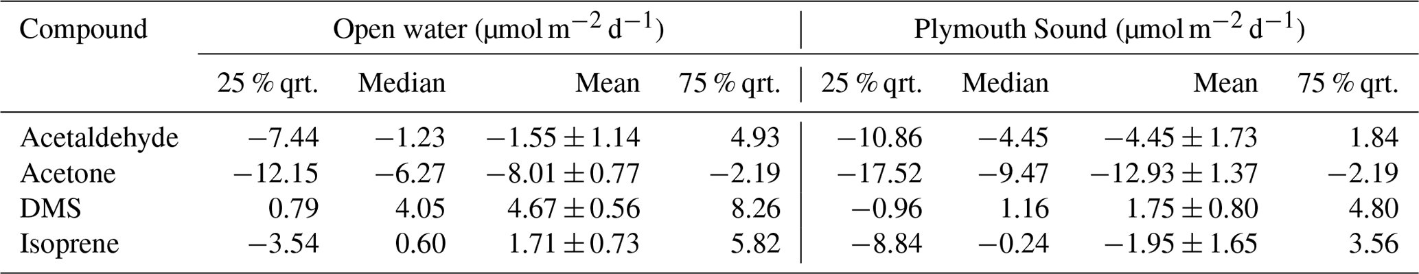
Mean EC (± 1 standard error) fluxes of acetone, acetaldehyde and DMS from the open-water wind sector were −8.0 ± 0.8, −1.6 ± 1.4 and 4.7 ± 0.6 µmol m−2 d−1 respectively (“−” sign indicates net air-to-sea deposition). These measurements are generally comparable (same order of magnitude) to previous measurements in the eastern North Atlantic Ocean at the same latitude. In comparison, the Plymouth Sound wind sector showed respective fluxes of −12.9 ± 1.4, −4.5 ± 1.7 and 1.8 ± 0.8 µmol m−2 d−1. The greater deposition fluxes of acetone and acetaldehyde within the Plymouth Sound were likely to a large degree driven by higher atmospheric concentrations from the terrestrial wind sector. The reduced DMS emission from the Plymouth Sound was caused by a combination of lower wind speed and likely lower dissolved concentrations as a result of the estuarine influence (i.e. dilution).
In addition, we measured the near-surface seawater concentrations of acetone, acetaldehyde, DMS and isoprene from a marine station 6 km offshore. Comparisons are made between EC fluxes from the open-water and bulk air–sea VOC fluxes calculated using air and water concentrations with a two-layer (TL) model of gas transfer. The calculated TL fluxes agree with the EC measurements with respect to the directions and magnitudes of fluxes, implying that any recently proposed surface emissions of acetone and acetaldehyde would be within the propagated uncertainty of 2.6 µmol m−2 d−1. The computed transfer velocities of DMS, acetone and acetaldehyde from the EC fluxes and air and water concentrations are largely consistent with previous transfer velocity estimates from the open ocean. This suggests that wind, rather than bottom-driven turbulence and current velocity, is the main driver for gas exchange within the open-water sector at PPAO (depth of ∼ 20 m).
- Article
(2112 KB) - Full-text XML
-
Supplement
(882 KB) - BibTeX
- EndNote


Volatile organic compounds (VOCs) are ubiquitous in the atmosphere and play an important role in atmospheric chemistry and carbon cycling in the biosphere (Heald et al., 2008). Many VOCs can influence the oxidative capacity of the atmosphere by acting as a source or sink of atmospheric ozone (O3) and hydroxyl radicals (Atkinson, 2000; Lewis et al., 2005), thereby influencing local air quality. The lower volatility oxidation products, produced from reactions of some VOCs with atmospheric oxidants, can condense into particulates and form cloud condensation nuclei (CCN) (Charlson et al., 1987; Blando and Turpin, 2000; Henze and Seinfeld, 2006), affecting the Earth's radiative forcing and climate.
The terrestrial environment is the largest source of VOCs to the atmosphere, with the emission dominated by isoprene from plant foliage (Guenther et al., 2006). Terrestrial biological processes also produce carbonyls, including ketones and aldehydes in varying amounts (Kesselmeier and Staudt, 1999). Large uncertainties exist however with respect to the role that the ocean plays as a net source or sink of these gases (Broadgate et al., 1997; Arnold et al., 2009; Millet et al., 2010; Fischer et al., 2012; Wang et al., 2019). This is due to poorly quantified air–sea fluxes as well as uncertainties in the biogeochemical and physical processes that control them.
Acetone and acetaldehyde are carbonyl-based VOCs that have been shown to make up to ∼ 57 % of the carbon mass of all non-methane organic carbon compounds in remote marine air over the North Atlantic Ocean (Lewis et al., 2005). These VOCs have been detected in the surface ocean at concentrations of up to tens of nanomolar (nM) (Zhou and Mopper, 1997; Williams et al., 2004), with known oceanic sources including the photochemical degradation of dissolved organic matter (DOM) in bulk seawater (Kieber et al., 1990; Zhou and Mopper, 1997; Zhu and Kieber, 2018) and possibly autotrophic/heterotrophic biological processes (Halsey et al., 2017; Schlundt et al., 2017). The heterogeneous oxidation of DOM at the sea surface has recently been identified as a source of carbonyl-containing VOCs (Zhou et al., 2014; Ciuraru et al., 2015); however the significance of this is currently unknown.
Dimethylsulfide (DMS) is a biogenic sulfur-containing VOC that constitutes the majority of the organic sulfur in the atmosphere (Andreae et al., 1985). It is produced in the surface ocean from the degradation of the algal osmolyte dimethylsulfoniopropionate (Kiene et al., 2000) and subsequently emitted into the atmosphere. DMS is often the dominant source of sulfur in the marine atmosphere (Yang et al., 2011b), and the oxidation products of DMS can act as CCN (Charlson et al., 1987; Veres et al., 2020).
Isoprene is an unsaturated terpene-based VOC that is produced in the ocean by a broad range of phytoplankton as a secondary metabolic product (Moore et al., 1994; Shaw et al., 2003; Exton et al., 2013; Booge et al., 2016; Dani and Loreto, 2017). Oceanic sources of isoprene are important for the remote marine atmosphere (Lewis et al., 2001; Arnold et al., 2009; Booge et al., 2016) where transport from terrestrial sources is negligible due to isoprene's very short atmospheric lifetime (∼ 30 min; Carslaw et al., 2000).
The main oceanic sink of most VOCs is biological metabolism at varying rates (Dixon et al., 2014; Royer et al., 2016; Halsey et al., 2017). Surface seawater concentrations of acetone and acetaldehyde tend not to be very sensitive towards their air–sea fluxes (Beale et al., 2015). Emission to the atmosphere is generally considered to be a small loss for seawater DMS (Yang et al., 2013b) but a much larger loss relatively for seawater isoprene (Booge et al., 2018).
There have been very few direct measurements of air–sea VOC fluxes with the eddy covariance (EC) technique (e.g. Marandino et al., 2005; Yang et al., 2013c, 2014b; Kim et al., 2017). More often, the fluxes are estimated with the bulk method using air and sea concentrations in a two-layer (TL) model (e.g. Baker et al., 2000; Beale et al., 2013; Wohl et al., 2020). Most studies focus on open ocean air–sea exchange, while air–sea VOC flux measurements from the coast are essentially non-existent (EC or bulk). Compared to the open ocean, the coastal waters tend to be very dynamic biogeochemically (Borges et al., 2005; Bauer et al., 2013) and physically. For example, riverine runoffs carry nutrients and organic carbon into the coastal seas, which could stimulate intense biological cycling (Cloern et al., 2014). Furthermore, compared to the remote marine atmosphere, coastal air is affected by terrestrial emissions.
The air–sea gas transfer velocity can be derived by equating the EC flux with the bulk TL flux (e.g. Blomquist et al., 2010; Bell et al., 2013; Yang et al., 2013a, 2014a). Limited studies have been undertaken to identify whether open-ocean-derived parameterisations of the transfer velocity are applicable to coastal systems (Borges et al., 2004; Yang et al., 2019a). Turbulent processes (i.e. wave-breaking, tidal currents, bottom driven turbulence) are expected to behave differently in these environments (Upstill-Goddard, 2006), with potential impacts on gas exchange.
Here we present air–sea fluxes of acetone, acetaldehyde and DMS determined using the EC technique at a coastal observatory in the south-west UK. Using seawater concentrations measured from a marine station 6 km offshore, we further compute the TL fluxes of these VOCs as well as the TL flux of isoprene. We compare our coastal flux measurements with previous observations of open ocean fluxes as well as global model estimates. From the EC fluxes and air and sea concentrations, we derive the gas transfer velocities of DMS, acetone and acetaldehyde and compare them against previous observations from the open ocean.
2.1 Location
The Penlee Point Atmospheric Observatory (PPAO) is a long-term monitoring station and a part of the Western Channel Observatory (WCO; https://www.westernchannelobservatory.org.uk/penlee/, last access: 20 May 2021) on the south-west (SW) coast of the UK (50.318∘ N, −4.189∘ E). The suitability of the observatory for direct air–sea exchange measurements (momentum, heat, greenhouse gases, sea spray aerosols, O3) has been discussed in detail before (Yang et al., 2016a, c, 2019a, b; Loades et al., 2020). The PPAO is located on an exposed headland that observes two distinct wind sectors representative of different air–sea exchange regimes. The SW open-water sector (depth of ∼ 20 m within the flux footprint) faces the western English Channel and North Atlantic Ocean. The north-east (NE) Plymouth Sound sector (fetch-limited with a depth of ∼ 10 m) is influenced by estuarine output from the rivers Tamar and Plym (Uncles et al., 2015) as well as natural terrestrial and anthropogenic atmospheric emissions. The theoretical extent of the flux footprint at the PPAO has been discussed previously (Yang et al., 2019a; Loades et al., 2020).
2.2 Set-up and measurements
The EC system here principally consists of a high-sensitivity proton-transfer-reaction mass spectrometer (PTR-quadrupole-MS, Ionicon Analytik) and a sonic anemometer (Gill Windmaster Pro). The measurement set-up closely followed previous PPAO flux campaigns (Yang et al., 2016a, d), with a few adaptations made to accommodate the PTR-MS requirements. A simple gas flow diagram is shown in Fig. 1.

Figure 1Schematic of the tubing set-up used to draw atmospheric sample to the gas instrument (PTR-MS). Dashed lines represent the set-up of the platinum catalyst before the synthetic gas blank was added. UT represents union tee, a three-way static connection.
The sonic anemometer was mounted on a mast ∼ 19 m above mean sea level and run at 10 Hz. The air inlet consisted of a downwards-facing 90∘ union, mounted 30 cm below the anemometer, connected via a 10 m tube to a union tee upstream of the air pump (UT1). All PPAO air sampling instruments (including the PTR-MS) subsampled ambient air from this union tee. A dry pump (Gast 1023 series) was used to draw ambient air into the observatory. The total flow rate was ∼ 13.5 L min−1, as calculated from the continuously monitored flow of the pump (Bronkhurst EL-FLOW series) and the sum of independent flows of connected instruments. All unions and tubing before UT1 were 9.5 mm internal diameter (ID).
Downstream of UT1 (i.e. closer to the instruments) was a 0.3 m, 3.2 mm ID tube and union tee (UT2), which split the sample air between the PTR-MS and other equipment (see Loades at al., 2020, for simultaneous PPAO O3 fluxes). Downstream of UT2 (i.e. closer to the PTR-MS) was a 0.3 m, 1.6 mm ID tube, which connected through a solenoid valve (Takasago Electric, Inc.) to the 1.2 m, 0.8 mm ID PTR-MS inlet tubing. All tubing, unions and fittings between the mast inlet and PTR-MS inlet were made from perfluoroalkoxy, while the solenoid valve was polytetrafluoroethylene, and the PTR-MS inlet was polyetheretherketone (heated to 80 ∘C to limit surface adsorption).
A solenoid valve, controlled from the PTR-MS, was used to automate routine hourly blanking for the VOC measurements. At the beginning of the campaign, sample gas (ambient air) was diverted through a platinum catalyst (heated to 450 ∘C) to produce VOC-free air (full oxidation to CO2; Yang and Fleming, 2019). However, the use of the catalyst caused overheating within the PPAO building and was replaced with an activated charcoal filter, which unfortunately proved to be inefficient at removing VOCs. The charcoal filter was replaced with compressed clean air (BOC synthetic air) towards the end of the campaign (27 April–3 May 2018), which yielded the most consistent blanks. Post-campaign experiments show that the acetaldehyde background when measuring dry, CO2-free compressed air is lower than measuring moist atmospheric air scrubbed by the catalyst by about 0.33 ppbv (Wohl et al., 2020). This difference is due to the different levels of CO2 (accounting for ∼ 0.3 ppbv) and to a lesser extent water vapour (accounting for ∼ 0.03 ppbv) between the compressed air and ambient air, qualitatively consistent with previous works (Warneke et al., 2003; Schwarz et al., 2009). Our calculation of atmospheric acetaldehyde mixing ratio accounts for these sensitivities. Overall, the determination of the VOC backgrounds was more uncertain during this campaign than in previous measurements (Yang et al., 2013c); however, this is not expected to significantly influence the EC fluxes since the air concentrations were detrended during the flux calculation (Sect. 2.4).
The PTR-MS was set to multiple ion detection mode with four VOCs of interest: acetaldehyde, acetone, DMS and isoprene (initially at 45, 59, 63 and 69 respectively). Previous experiments (Schwarz et al., 2009) and our laboratory tests (Wohl et al., 2019) show that substantial isoprene fragmentation occurs at the voltage used in these measurements (690 V, 166 Td). Importantly, the 41 fragment ion was shown to provide a larger and more stable signal than that of the isoprene parent ion ( 69). As a result, a week into the campaign, the monitoring of isoprene was changed to 41. The calibration (Sect. 2.5) and thus calculation of the isoprene mixing ratio accounted for the fragmentation and the change in ion monitored. The quadrupole mass dwell time was set to 50 ms for H3O+ and 100 ms for each VOC. In total, the full ion cycle was just over 450 ms, which resulted in a sampling frequency of 2.2 Hz. Dwell time for each VOC was a compromise between measurement frequency and instrument noise. The PTR-MS parameters are listed in Table A1. Data from the sonic anemometer, flow meter and PTR-MS were all recorded on the same computer to avoid desynchronisation.
2.3 Eddy covariance flux calculation
EC gas fluxes (F) are determined from the correlation between rapid changes (at least a few Hz) in vertical wind velocity (w) and the gas mixing ratio (x); , where ρa represents dry air density, the primes represent fluctuations from the mean and the overbar represents temporal averaging. Air density was computed using the PPAO air temperature, pressure and humidity data (Gill Instruments Metpak Pro). Wind measurements were linearly interpolated from 10 Hz to match VOC measurement frequency.
A double wind rotation (Tanner and Thurtell, 1969; Hyson et al., 1977) was applied to each 10 min segment of wind data (u and v= horizontal, w= vertical), such that u became the wind speed (U) in the mean wind direction, and v and w each averaged zero. This was done to minimise the effect of flow distortion caused by the headland.
A lag time of approximately 3.5 s between wind and PTR-MS measurements was calculated from the dimensions of the tubing and flow rate. The lag time was further determined hourly using a lag correlation analysis between w and x over a window of +10 s. Acetone had the strongest flux signal of the four VOCs measured and was used to determine the lag time.
Lag-adjusted PTR-MS data were used to calculate fluxes in 10 min segments, the sampling interval chosen as the best compromise between maintaining sufficient flux signal-to-noise ratio and satisfying the stationarity criteria in this dynamic region (Yang et al., 2016a, c, 2019a, b).
The sampling frequency of the PTR-MS is relatively low (2.2 Hz), and the instrument's response time determined from laboratory tests is just under 0.5 s. The computed fluxes were corrected for high-frequency signal loss due to (1) sampling at 2.2 Hz, and thus missing the flux above the Nyquist frequency of 1.1 Hz, and (2) attenuation due to the tubing, using a combined wind-speed-dependent attenuation factor (mean 1.09, max 1.18). This signal attenuation was estimated from the instrument's response time following the approach of Yang et al. (2013a).
The 10 min flux segments that met the quality control criteria (Table A2 for criteria details) were averaged into 1 h or 3 h fluxes, which reduces random noise by a factor of ∼ and ∼ , respectively. Over the entire duration of the campaign, 61 % of the data were discarded, mainly due to inappropriate wind directions (i.e. from land) or large variability in wind direction (more common at low wind speeds). Diurnal variability was apparent in the open-water wind sector data (SW winds) with respect to the number of acceptable flux segments. About twice as many flux segments passed quality control in the daylight hours compared to at night, which is likely due to a diurnal sea-breeze effect. When EC fluxes were averaged across 5 weeks of measurements, no difference was observed per hour of the day. No diurnal cycle could be seen in the Plymouth Sound wind sector data (NE winds), likely in part due to the limited data size.
Co-spectra of acetone and DMS averaged over all quality-controlled periods are shown in Fig. 2 for both the open-water and Plymouth Sound wind sectors. Here the areas between the co-spectral curves and zero represent the magnitudes of the fluxes. Theoretical co-spectral fits constrained by the actual wind speed and measurement height (Kaimal et al., 1972) suggest that the measured co-spectral shapes were reasonable. The Kaimal fits also showed the high-frequency flux loss (≳ 1 Hz) was small, consistent with the estimated high-frequency signal loss correction. Acetaldehyde and isoprene are not shown here because the bidirectionality in acetaldehyde flux and the low isoprene flux magnitude (Sect. 3.1) cause very noisy co-spectra.
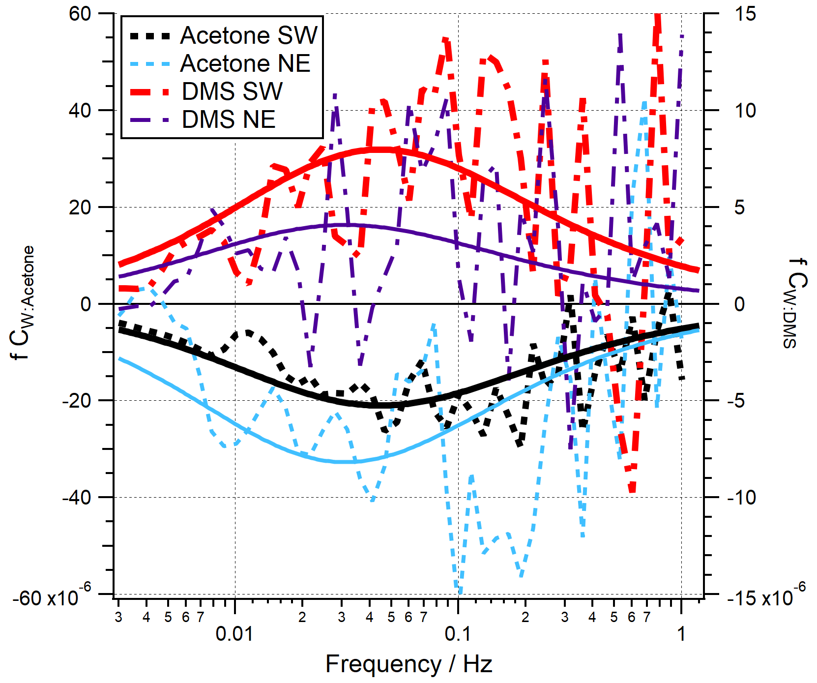
Figure 2Mean flux co-spectra for acetone and DMS in the SW and NE wind sectors. Dashed/broken lines represent PPAO observations. Solid lines represent the idealised spectral fits (Kaimal et al., 1972), where measurement height and wind speed are specified according to the measurement conditions.
2.4 Seawater measurements and two-layer flux calculation
Discrete seawater samples were collected from the L4 marine time-series station of the WCO, which is ∼ 6 km S–SW of the PPAO headland. The near-surface VOC concentrations are presumed to be similar between L4 and the PPAO open-water flux footprint despite the outflow from the Tamar estuary that hugs the PPAO headland (Uncles et al., 2015); we revisit this assumption in Sect. 3.3. Seawater acetaldehyde, acetone, DMS and isoprene concentrations were determined using a segmented flow coil equilibrator coupled to the PTR-MS before and after the PPAO campaign (following Wohl et al., 2019). Additional seawater DMS concentration measurements were made weekly at L4 using gas chromatography (following Hopkins and Archer, 2014) for the March–May 2018 period.
Atmospheric VOC mixing ratios were blank-corrected using the synthetic gas cylinder measurements (27 April 2018 onwards; see Sect. 2.2), accounting for the humidity dependence in the background of DMS (mean correction 0.22 and 0.12 ppbv, for SW and NE air respectively, estimated from Wohl et al., 2019) and the CO2 plus humidity dependences in the background of acetaldehyde (constant correction 0.33 ppbv estimated from data from Wohl et al., 2020). We have greater confidence in the measured atmospheric VOC mixing ratios after switching to synthetic air for the blank measurement. Thus, the EC fluxes and the two-layer (TL) bulk fluxes were compared over this period (27 April–3 May 2018) only. Gas-phase calibrations of the PTR-MS (using a certified gas standard, Apel–Riemer Environmental Inc) before and after the deployment were averaged and applied to both the atmospheric and seawater VOC data.
Surface saturation values of DMS and acetaldehyde were calculated using the recommended solubility from the literature (Burkholder et al., 2015; Sander, 2015) as a function of temperature and adjusted for salinity (Johnson, 2010). Recent calibrations at environmentally relevant concentrations in seawater suggest that acetone is less soluble than previously thought (Wohl et al., 2020); thus the acetone air-over-water solubility recommended by Burkholder et al. (2015) was by divided by 1.4, as recommended by Wohl et al. (2020).
The calculation of the bulk TL fluxes requires the use of wind-speed-dependent gas transfer velocity parameterisations. The measured wind speed at the PPAO was corrected for flow acceleration due to the headland using results from a comparison with a wind sensor on the L4 buoy (Yang et al., 2019a). This scaled the wind speeds from 19 m (height of the PPAO mast) to 4.9 m (height of L4 wind sensor) and also removed the effect of wind acceleration from the sloped PPAO headland. The corrected winds were then scaled to 10 m; , where z0 represents the aerodynamic roughness length calculated from U using the COAREG 3.5 model (Edson et al., 2013). Overall, the mean correction factor was 0.93 (min 0.79 and max 1.39) for the two wind sectors. The relationship between the corrected U10 and EC friction velocity, , shows reasonable agreement with the COAREG 3.5 model as well as with Mackay and Yeun (1983) (Fig. S1), which validate these wind corrections.
Bulk fluxes (F) were calculated following Liss and Slater (1974) and Johnson (2010):
where Ka represents total airside transfer velocity, Ca and Cw represent air- and waterside concentrations respectively, H represents air-over-water dimensionless Henry solubility, and ka and kw represent the individual air and waterside transfer velocities, respectively. Note that total waterside transfer velocity (Kw), more commonly used for waterside controlled gases such as DMS and isoprene, is equal to HKa. ka was calculated from the COAREG 3.5 model (Edson et al., 2013), which can be approximated as . The VOCs targeted here span only a small range in diffusivity in air and are thus assumed to have the same ka for simplicity (Yang et al., 2014a, 2016b). kw for acetone, acetaldehyde and DMS was calculated using the fit from Yang et al. (2011a); this was an average of DMS observations from five cruises: , where SCw represents the waterside Schmidt number. kw for isoprene was calculated using the fit from Nightingale et al. (2000); . At a U10 of 10 m s−1, the Nightingale et al. (2000) parameterisation would overestimate DMS kw by ∼ 37 % because bubble-mediated gas exchange is less important for the moderately soluble DMS (see Bell et al., 2017; Blomquist et al., 2017). The waterside Schmidt number for all gases was computed following Johnson (2010) at the ambient temperature and salinity.
Appendix B provides further information on the chosen gas solubilities, waterside data and calculations.
Table 1Eddy covariance flux measurements over the entire campaign. Errors indicate standard errors (SEs) with n=135 and n=40 bins (1 h averages) for the open-water and Plymouth Sound sectors respectively. Also included are the quartiles (qrt).
3.1 EC fluxes for the open-water and Plymouth Sound wind sectors
Flux measurements were made between 5 April and 3 May 2018. During this period, winds arrived from the open-water wind sector (180–240∘ N) 30 % of the time and from the Plymouth Sound sector (30–70∘ N) 8 % of the time. The wind directions defining these two marine flux sectors were re-established (see Appendix C) compared to previous PPAO studies after raising the mast height by ∼ 1 m at the beginning of this campaign.
A time series of VOC fluxes (3 h average) is shown in Fig. 3. While acetone and DMS had clear unidirectional fluxes (deposition and emission respectively), acetaldehyde showed bidirectional fluxes throughout the campaign. EC fluxes of acetone, acetaldehyde, DMS and isoprene from the two marine wind sectors averaged over the entire campaign are summarised in Table 1, with positive fluxes representing net sea-to-air emission.
For the open-water sector, acetone and DMS fluxes had relative standard errors <12 % (from 1 h bins), which are confidently represented by the measurements in the mean thanks to the robust signal-to-noise ratio. Acetaldehyde had a much greater relative standard error (74 %) because the fluxes often changed in direction and were smaller in magnitude (closer to the limits of detection, LOD); acetaldehyde standard error is lowered to 51 % when the 573 10 min flux segments are instead averaged over the campaign. The isoprene flux was not resolvable with the EC method using our PTR-MS due to the low signal-to-noise ratio. The only direct measurement of isoprene flux from the sea (Kim et al., 2017, in the North Atlantic Ocean) used a chemical ionisation mass spectrometer that is significantly more sensitive than the PTR-MS here.
Overall, 68 %, 33 %, 62 % and 35 % of 3 h averages of acetone, acetaldehyde, DMS and isoprene, respectively, were above the LOD (DMS and isoprene had the additional condition of a positive flux above LOD) for the open-water sector. The estimation of LOD is shown in Appendix A.
The greater air-to-sea deposition fluxes of acetone and acetaldehyde in the Plymouth Sound sector, compared to the open-water sector, were likely driven by the higher gas mixing ratios in terrestrially influenced air. Distributions of atmospheric acetone mixing ratio from the two wind sectors are shown in Fig. 4. Seawater concentrations of acetone and acetaldehyde within the Plymouth Sound flux footprint were not measured, and thus we are unable to comment on the quantitative effect of riverine outflow on the dissolved VOC concentrations. The weaker sea-to-air flux of DMS in the Plymouth Sound sector compared to the open-water sector was likely due to a combination of low DMS water concentrations associated with freshwater outflow (Uncles et al., 2015) and lower wind speed (Fig. 4) that results in reduced gas transfer velocity (kw; Nightingale et al., 2000; Yang et al., 2011a).

Figure 3Time series of 3 h averages of (a) wind speed (U10) and wind direction, (b) acetaldehyde flux, (c) acetone flux and (d) DMS fluxes for the open-water (180–240∘ N) and Plymouth Sound (30–70∘ N) wind sectors that met quality control criteria. Error bars are 1 standard error. The blue and green shaded zone in panel (a) represent the two wind sectors. The grey shaded zones in panels (b)–(d) represent limits of detection for 3 h averages, 5.8, 4.0 and 2.7 µmol m−2 d−1 for acetaldehyde, acetone and DMS respectively.

Figure 4Histogram of (a) wind speed (U10) and (b) acetone and (c) DMS atmospheric gas-phase mixing ratio over the entire campaign. Histograms are normalised for probability density separately and then to the same relative maximum occurrence. The gas mixing ratio calculations here use extrapolated blanks here, which introduce some uncertainty; however the two wind sectors can still be compared.
3.2 Seawater concentration and atmospheric mixing ratios of VOCs
The seawater concentrations of acetone, acetaldehyde and DMS measured around the campaign (Table A4) are broadly similar (≤ 48 % difference) to previous measurements in the western English Channel (Archer et al., 2009; Beale et al., 2015), a highly variable and seasonal environment. No seawater measurements of isoprene have been published in this region, so comparisons are made to previous observations from the eastern North Atlantic (∼ 0.02 nM; Broadgate et al., 2004; Hackenberg et al., 2017), which are ∼ 79 % lower than measurements here. The eastern North Atlantic measurements were conducted in September–October, thus likely represent a period of lower isoprene productivity. An annual study in the North Sea found the highest isoprene seawater concentrations in May (∼ 0.06 nM; Broadgate et al., 1997), which were closer to our L4 measurements but still lower (∼ 41 %).
The mean atmospheric mixing ratios of acetone and acetaldehyde from the open-water sector (0.82 ± 0.16 and 0.51 ± 0.07 ppbv respectively, Table 2) are greater than previous measurements around the sample site, possibly in part due to our measurements occurring mainly over 1 d (1 May 2018; see Fig. 6 later for time series); thus a multi-day average was not possible. Remote marine Atlantic Ocean measurements from the ATom-4 campaign (April–May 2018), within 0.5 km of the sea surface and at latitudes of 40–60∘ N, observed 0.31 ± 0.01 ppbv acetone (± SD) and 0.15 ± 0.04 ppbv acetaldehyde (Wofsy et al., 2018). Better agreement was seen with shipboard measurements between 40 and 50∘ N in the eastern North Atlantic Ocean (Yang et al., 2014b) and coastal measurements at the Mace Head Observatory (Lewis et al., 2005), with mean acetone mixing ratios of ∼ 0.65 and 0.50 ppbv, respectively, and acetaldehyde mixing ratios of ∼ 0.16 and 0.44 ppbv, respectively. Finally, rooftop measurements at PML (∼ 350 m north of the Plymouth Sound, ∼ 6 km NE of the PPAO, and affected by local ship/port activities) showed night-time atmospheric mixing ratios of ∼ 0.4 and ∼ 0.1 ppbv, respectively for acetone and acetaldehyde (Yang et al., 2013c). A summary of these concentrations, in coordinate form, can be found in Fig. S3. The atmospheric carbonyl measurements at the PPAO from this day might not represent purely oceanic conditions, even though wind was from the open-water sector. HYSPLIT (Stein et al., 2015; Rolph et al., 2017) backward trajectories suggest that the air mass sampled on 1 May 2018 made contact with land (mainland UK) ∼ 24–48 h prior to arriving at the PPAO (Fig. S4). Lewis et al. (2005) show that similar air-mass trajectories over the UK and continental Europe contained high acetone levels (max of ∼ 1.67 ppbv).
Our mean DMS mixing ratio (0.20 ± 0.09, Table 2) is in agreement with shipboard measurements in the eastern North Atlantic Ocean in June and July (0.16 ± 0.14 and 0.12 ± 0.08 ppbv, with and without a phytoplankton bloom, respectively; Huebert et al., 2010) and the western North Atlantic Ocean in March (0.13 ± 0.04; Quinn et al., 2019). Our mean isoprene mixing ratio (0.18 ± 0.05) is higher than observations in autumn from the western North (0.035 ± 0.025 ppbv; Kim et al., 2017) and eastern North (0.0044 ± 0.0083 ppbv; Hackenberg et al., 2017) Atlantic Ocean. The PPAO isoprene mixing ratio is more similar to measurements at the Mace Head Observatory (Carslaw et al., 2000), which further implies some influence from terrestrial land sources at the PPAO site. We note that the TL air–sea isoprene flux is almost purely governed by its seawater concentration where it is grossly supersaturated; the flux is insensitive to the elevated atmospheric mixing ratio.
3.3 Comparison between EC and bulk TL fluxes and derivation of the gas transfer velocities
Here we compare EC fluxes of acetone, acetaldehyde and DMS from the open-water sector with fluxes computed with the TL model (using concurrent atmospheric mixing ratios from the PPAO and linearly interpolated seawater concentrations from L4). This is to assess two assumptions in the TL flux calculation: (1) that gas transfer velocity parameterisations from deeper water (i.e. the open ocean or shelf seas) are applicable to this shallower coastal environment, and (2) seawater VOC concentrations in the PPAO flux footprint and at the L4 station are similar.
Acetone and acetaldehyde were both undersaturated in seawater in the open-water sector (Table 2), while DMS and isoprene were both supersaturated. The mean TL fluxes of acetone, acetaldehyde, DMS and isoprene (n=20) are provided in Table 2 with corresponding EC measurements from the open-water wind sector for the last week of the campaign (27 April–3 May 2018). For this short period with satisfactory VOC blanking, the open-water EC fluxes were fairly large in part because of a 17 % higher mean wind speed compared to the rest of the campaign.
Figure 5 compares the VOC EC and TL fluxes for the open-water sector (not inc. isoprene), and Fig. 6 shows the same data as a time series. Acetone, acetaldehyde and DMS fluxes exhibit reasonable agreement between the EC and TL methods, with both covarying with wind speed. The data points furthest from the 1:1 line in Fig. 5 are hourly averages with ≤ 2 10 min flux segments, suggesting that the discrepancy is mainly due to random noise in the flux measurement. We do not attempt to calculate TL fluxes for the Plymouth Sound sector because we do not have concurrent seawater measurements and have limited EC measurements for comparison.
Table 2Saturations and two-layer bulk fluxes of VOCs in open-water (SW) and Plymouth Sound (NE) water (27 April–3 May 2018) along with the eddy covariance measurements for this period. Errors for water concentration and air mixing ratio (measurement) and saturation (propagation) indicate one standard deviation. Errors for flux indicate one standard error.
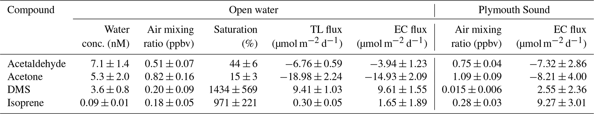
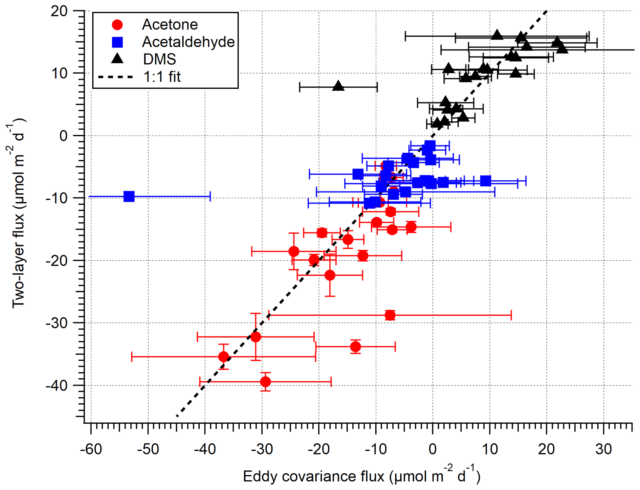
Figure 5A comparison between EC and bulk TL fluxes (hourly) for the open-water sector during the dates 27 April–3 May 2018. The error on EC measurements is 1 SE, whilst the error on TL is the propagated error of 1 SD in concentration and solubility.
To assess the wind speed dependence in gas transfer velocities at the PPAO, Ka is calculated by equating the EC flux with TL flux; . Figure 7 shows the calculated Ka and Kw (Kw=HKa) values for acetone, acetaldehyde and DMS using 1 h flux data, compared to calculated K from parameterisations of ka and kw. In the mean, the expected solubility dependence in these VOCs is observed – the measurements show mean Ka of 2121, 1894 and 183 cm h−1 for acetone, acetaldehyde and DMS (in order of decreasing solubility), respectively. These translate to Kw values of 2.0, 2.6 and 9.9 cm h−1.
For DMS, to facilitate comparison with previous measurements, the derived Kw is adjusted to a standard Schmidt number of 660 (). The mean K660 for DMS (16.7 ± 2.7 cm h−1) is in good agreement when compared to published measurements (∼ 17 cm h−1; Blomquist et al., 2006; Yang et al., 2011a; Bell et al., 2013) at similar wind speeds in the North Atlantic Ocean. Data from this short campaign suggest that the mean wind speed dependence in DMS transfer velocity at the PPAO (open-water sector, depth of ∼ 20 m) is largely comparable to deeper water, in agreement with previous CO2 gas exchange measurements at this site (Yang et al., 2019a). Our measured acetone and acetaldehyde Ka are also of the expected magnitudes. Processes important for shallow estuaries, such as bottom-driven turbulence and tidal current, do not appear to be the main controlling factors in gas exchange in this environment.
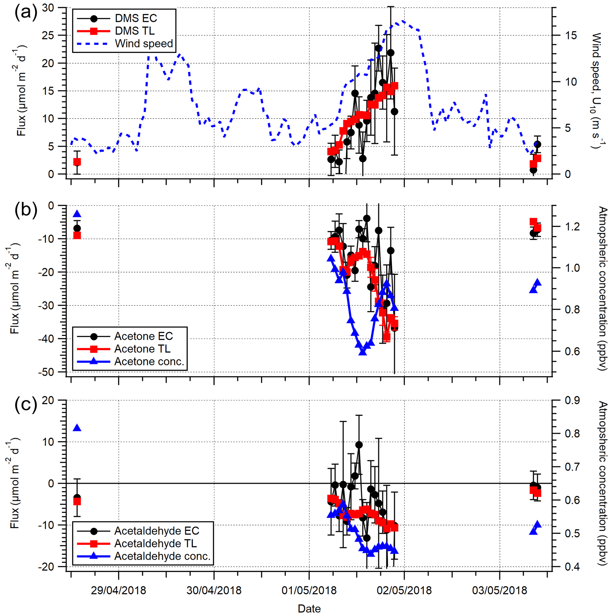
Figure 6A comparison between (a) DMS, (b) acetone and (c) acetaldehyde EC and TL fluxes (hourly) for the open-water sector during the dates 27 April–3 May 2018. Wind speed (U10) is provided in (a). The error on EC measurements is 1 SE, whilst the error on TL is the propagated error of 1 SD in concentration and solubility.
There is a large amount of scatter in Fig. 7, especially for acetone and acetaldehyde. This is likely in part due to the poor temporal resolution (weekly) in seawater concentration measurements that do not capture any rapid changes in this dynamic region (e.g. changes in riverine outflow, biological bloom). Our DMS transfer velocity measurements imply that the outflow of the estuary Tamar does not substantially dilute the seawater DMS concentration within the open-water flux footprint compared to L4, while spatial gradients in the carbonyl concentrations could be more significant relative to their air–sea concentration differences. Higher resolution measurements within the flux footprints in the future are needed to better constrain the influence of riverine outflow.

Figure 7Calculated transfer velocities (hourly) for (a) DMS (Kw,600), (b) acetone (Ka) and (c) acetaldehyde (Ka) in the open-water footprint of the Penlee Point Atmospheric Observatory during the dates 27 April–3 May 2018. Error bars on the experimental data (black circles) are propagated uncertainty from the eddy covariance measurement. The black poly fit lines are fit to the experimental data, with the dashed black lines representing 95 % confidence in the poly fit. The red circle and blue triangle lines in panel (a) are theoretical transfer velocities using the kw parameterisations of Yang et al. (2011a) and Nightingale et al. (2000) respectively. The red circle lines in panels (b) and (c) are theoretical transfer velocities calculated from the kw parameterisation of Yang et al. (2011a) and ka from the COAREG 3.5 model (shown as blue triangles).
As mentioned in Sect. 2.5, this paper uses a revised acetone solubility from Wohl et al. (2020). Focusing on the last week of the campaign (Table 2), we compute a mean TL acetone flux of −19.0 ± 2.2 and −21.5 ± 2.5 µmol m−2 d−1 (± SD, propagated error in concentration only) with and without the solubility revision. The flux with revised solubility is in better agreement with the EC measurement (−14.9 ± 2.1 µmol m−2 d−1).
3.4 Comparison to other flux estimates
The acetone fluxes presented here are in good agreement with previous EC measurements (−7.0 ± 2.2 µmol m−2 d−1) from 50∘ N on an Atlantic Meridional Transect (AMT) research cruise in Autumn 2012 (Yang et al., 2014b). However, the acetaldehyde flux here shows an opposite mean direction to their 50∘ N average (1.8 ± 1.3 µmol m−2 d−1). Acetone and acetaldehyde bulk fluxes from 50∘ N during an AMT cruise in 2009, estimated using CAM-Chem modelled atmospheric concentrations, were −5.7 ± 1.1 and −2.4 ± 0.7 µmol m−2 d−1 respectively (Beale et al., 2013). The PPAO fluxes are in reasonable agreement with these earlier indirect estimates. Further acetone and acetaldehyde bulk fluxes estimated from a time series of L4 water measurements and static atmospheric mixing ratios (0.66 and 0.40 ppbv respectively) were −7.4 ± 1.4 and 1.4 ± 1.0 µmol m−2 d−1, respectively, for spring 2011 and −6.4 ± 0.1 and −1.5 ± 0.1 µmol m−2 d−1, respectively, as annual averages. The spring acetone fluxes of Beale et al. (2015) are in good agreement with the PPAO direct measurements; however their acetaldehyde flux was in the opposite direction. Importantly, Beale et al. (2015) identified that the L4 water saturation of acetaldehyde was highly sensitive to the atmospheric mixing ratio (changing it between 0.1–0.4 ppbv was enough to switch the direction of flux). Thus variability and uncertainty in the atmospheric acetaldehyde mixing ratio are probably among the main causes for the discrepancies in these air–sea flux estimates (Yang et al., 2014b, Beale et al., 2013, 2015, and PPAO measurements presented here).
The PPAO DMS flux is in agreement with previous EC DMS flux observations from the eastern North Atlantic Ocean during summer 2007 (4.4 ± 0.4 and 2.6 ± 0.2 µmol m−2 d−1 with and without a short, intense phytoplankton bloom; Huebert et al., 2010). Our campaign ended before the spring phytoplankton bloom started at L4 (Archer et al., 2009), which typically starts in May or June. Yang et al. (2016c) estimated bulk DMS fluxes of 3 and 10 µmol m−2 d−1 in the winter and summer, respectively, using the L4 annual seawater DMS concentration time series (Archer et al., 2009). The DMS flux measurement at the PPAO is also in reasonable agreement with previous observations in the North Atlantic Ocean without the phytoplankton bloom (5.58 ± 0.15 µmol m−2 d−1; Bell et al., 2013).
Although isoprene EC fluxes were unresolvable, the estimated open-water TL flux was similar to NECS April estimates of ∼ 0.8 µmol m−2 d−1 (Palmer and Shaw, 2005) and ∼ 1.0 µmol m−2 d−1 (Booge et al., 2016, supplement) using MODIS satellite observations of chlorophyll a for production models. A mean direct flux (0.7 µmol m−2 d−1) was observed in the northern North Atlantic Ocean (Kim et al., 2017); Kim et al. (2017) estimated seawater concentrations (∼ 0.02 nM) that were ∼ 78 % lower than measured here but also experienced much higher wind speed. Importantly, discrepancies between top-down and bottom-up isoprene budget analyses show the ocean fluxes necessary to explain remote marine boundary layer (MBL) concentrations of isoprene are an order of magnitude higher than predicted from seawater concentrations alone (Arnold et al., 2009; Booge et al., 2016). Future simultaneous comparisons between EC and TL isoprene fluxes might observe this difference.
We also compare our direct VOC fluxes to global model predictions at this location. Typical global models and climatologies operate with a 1∘ latitudinal and longitudinal resolution (e.g. Wang et al., 2019, 2020a, b). At the PPAO, this equates to a grid size of ∼ 110 km N–S and ∼ 85 km E–W, which is much coarser compared to the flux footprint areas (on the order of a few square kilometres). Nevertheless, this comparison allows us to qualitatively assess the spatial representativeness of the PPAO fluxes and identify potential shortcomings in the models.
The GEOS-Chem and CAM-Chem models predict a mean annual acetone flux in the eastern North Atlantic Ocean coastal shelves (NECS; biogeochemical province that includes the PPAO coastal site) of ∼ −2.5 µmol m−2 d−1 (Fischer et al., 2012) and March–May flux of ∼ −2.9 µmol m−2 d−1 (Wang et al., 2020a), respectively. These two predictions are much lower than measured in the PPAO open-water sector (−8.01 ± 0.77 µmol m−2 d−1, Table 1) because the models predict a smaller air–sea concentration difference. Fisher et al. (2012) and Wang et al. (2020a) used water concentrations of 15 (static) and ∼ 8 nM respectively (182 % and ∼ 50 % higher than L4 concentrations) and a modelled atmospheric mixing ratio of ∼ 0.45 ppbv (∼ 45 % lower than the PPAO concentration). Seawater acetone has a highly variable lifetime (Beale et al., 2013; de Bruyn et al., 2013; Dixon et al., 2013), so the higher estimated seawater concentration in the Wang et al. (2020a) model may be because of a slower removal rate. We measured an atmospheric acetone mixing ratio that is higher than in the model likely because our measurement, even from the open-water sector, has some terrestrial influence (e.g. via the diurnal sea-breeze effect or advection of air masses previously in contact with land).
The small negative acetaldehyde fluxes measured at the PPAO imply a weak ocean sink (mean of −1.55 ± 1.14 µmol m−2 d−1, Table 1), which does not agree with global model results. The NECS acetaldehyde flux is ∼ 0.22 µmol m−2 d−1 in GEOS-Chem (Millet et al., 2010) and ∼ 1.4 µmol m−2 d−1 in CAM-Chem (Wang et al., 2019) in the March–May period. The seawater concentrations used by Wang et al. (2019) (∼ 11 nM) are higher than L4 measurements for the same period (54 % higher than L4 conc.). In the model, the short marine lifetime of acetaldehyde (de Bruyn et al., 2013, 2017; Dixon et al., 2013) is coupled with an estimate of its production rate to predict the seawater concentration. Wang et al. (2019) use of a constant lifetime of 0.3 d for the global ocean, whereas previous measurements at L4 suggest a much shorter acetaldehyde lifetime (0.01–0.13 d; Beale et al., 2015). de Bruyn et al. (2017) showed shorter seawater acetaldehyde lifetimes at another coastal location directly after rainfall or during the wet season. It is possible that the shorter lifetime at L4/PPAO, and hence lower seawater acetaldehyde concentration, may be related to riverine input. The atmospheric acetaldehyde mixing ratios from the models are also lower than the coastal observations presented here, similar to acetone as discussed above.
From the perspective of climatology and global modelling, the NECS was predicted to have an April DMS flux of ∼ 14 µmol m−2 d−1 (Lana et al., 2011) and ∼ 6 µmol m−2 d−1 (Wang et al., 2020b). The estimate of Lana et al. (2011) is 3 times higher than the PPAO measurements; however that of Wang et al. (2020b) is in good agreement. Waterside concentrations of ∼ 7 and ∼ 3 nM were predicted (52 % higher and 43 % lower than the L4 concentration) by Lana et al. (2011) and Wang et al. (2020b) respectively. The high concentrations in the Lana et al. (2011) climatology likely correspond to phytoplankton blooms in the April–May period, which did not occur at the time of our measurements or appear as intensely in the estimations of Wang et al. (2020b). This could be partly related to the interannual variability in plankton dynamics and hence seawater DMS cycling.
All the models and climatologies discussed here (except for Wang et al., 2020b) used the Nightingale et al. (2000) kw parameterisation, which leads to ∼ 26 %, ∼ 14 % and ∼ 26 % higher kw values for acetone, acetaldehyde and DMS, respectively, than those of Yang et al. (2011a) over this campaign because of the solubility dependence in bubble-mediated gas exchange (Yang et al., 2011a; Bell et al., 2017). Substituting the Nightingale et al. (2000) kw parameterisation with the Yang et al. (2011a) kw would generally reduce the flux magnitude in these models, estimated as ∼ 5 %, ∼ 6 % and ∼ 19 % for acetone, acetaldehyde and DMS, respectively (ka unchanged and from COAREG 3.5).
3.5 Significance of fluxes
Our measured open-water acetone and acetaldehyde air–sea fluxes exhibit stronger deposition flux than estimated by global modelling. Here we evaluate the lifetimes of these gases within the atmospheric MBL. The MBL lifetimes (τx) are calculated similarly to a 0D model; , where Cx represents concentration (here, the mean of the PPAO observations; Table 2), Lx represents chemical loss, Dx represents the net deposition flux (here, the mean of the PPAO EC observations; Table 1) and h represents MBL height. We assume h to be 500 m and VOCs to be homogeneously mixed within the MBL upwind of the PPAO, and Lx is 2.7 × 10⁻⁷ s−1 for acetone and 2.1 × 10⁻⁵ s−1 for acetaldehyde. Lx is calculated from literature OH reaction rates (1.7 × 10⁻¹³ and 1.5 × 10⁻¹¹ cm3 molec.−1 s−1, respectively; Atkinson and Arey, 2003), April surface 50∘ N zonal average OH concentration (∼ 106 molec. cm−3; Horowitz et al., 2003) and summer surface photolysis rates for acetone (∼ 10−7 s−1; Blitz et al., 2004) and acetaldehyde (∼ 5.5 × 10⁻⁶ s−1; Warneck and Moortgat, 2012).
From this simple model and the values described above, the MBL lifetimes of acetone and acetaldehyde are calculated to be 2.0 and 0.5 d respectively. The deposition to the ocean above accounts for 95 % and 8 % of all losses for MBL acetone and acetaldehyde respectively, which highlights the importance of acetone air–sea exchange. The calculated PPAO open-water acetone lifetime is much shorter than the 11–18 d estimates for the mean troposphere (Marandino et al., 2005; Fischer et al., 2012; Khan et al., 2015; Wang et al., 2020a), where surface deposition is less substantial (16 %–56 %; Jacob et al., 2002; Fischer et al., 2012). The acetaldehyde lifetime is in good agreement with literature values (0.1–0.8 d; Millet et al., 2010; Wang et al., 2019) because photochemistry is the main loss mechanism for MBL acetaldehyde rather than deposition, and the April surface 50∘ N zonal average OH concentration is similar to the tropospheric mean (1.1 × 10⁶ molec. cm−3; Li et al., 2018).
The noticeable increase in acetone and acetaldehyde deposition fluxes within the Plymouth Sound compared to the open-water sector suggests that deposition can represent a large loss term for atmospheric VOCs in the coastal atmosphere. Importantly, enhanced coastal deposition fluxes of acetone and acetaldehyde are not well captured in global models. The boundary layer lifetimes during periods of offshore winds are calculated using the same approach as before, resulting in 1.7 d for acetone and 0.5 d for acetaldehyde. Here deposition to the ocean accounts for 96 % and 17 % of losses, respectively. The estimated lifetimes in the Plymouth Sound sector are similar to the open ocean even though the deposition fluxes were stronger because the increased deposition fluxes correspond to a greater atmospheric burden. As air masses from the Plymouth Sound (or further inland to the NE) are advected offshore over the coastal seas, the mixing ratios of carbonyls tend to decrease due to combination of deposition to the sea, chemical losses and mixing with marine air. If additional x–y dimensional constraints are added to the Plymouth Sound 0D box (e.g. 4 km N–S, 1 km E–W), dilution becomes an important loss term.
This paper presents measurements of air–sea fluxes of acetone, acetaldehyde and DMS at the coastal PPAO in the SW UK. A PTR-quadrupole-MS (2.2 Hz) was used to simultaneously resolve the fluxes of these gases with the eddy covariance method. Comparisons between the open-water sector and a terrestrially influenced sector show stronger deposition fluxes of acetone and acetaldehyde from the latter because of higher atmospheric carbonyl concentrations from that wind direction. Emission fluxes of DMS from the terrestrially influenced sector are weaker than from the open-water sector, likely because of lower wind speeds and lower seawater concentrations due to estuarine influence/dilution.
Bulk fluxes computed from seawater and atmospheric concentrations using the TL approach agree reasonably well with our EC measurements of open-water acetone, acetaldehyde and DMS fluxes. The derived air–sea transfer velocities of acetone, acetaldehyde and DMS are largely consistent with previous estimates over the open ocean in the mean. Along with previous measurements of air–sea CO2 exchange, these data suggest that wind, rather than processes such as bottom driven turbulence, is the dominant control for gas exchange at this site for the open-water sector (depth of ∼ 20 m).
While the DMS flux at PPAO was in reasonable agreement with recent climatological estimates, our measured open-water acetone fluxes show stronger deposition compared to climatological and model estimates for the NE Atlantic Ocean coastal shelf. This is likely because the models/climatologies do not fully capture the spatial and temporal variability in the distribution of atmospheric and seawater acetone concentrations. The PPAO acetaldehyde flux (net sink in the mean) is in the opposite direction to global models that suggest the Northern Hemisphere oceans to be a net acetaldehyde source. This is mostly because models predict higher seawater acetaldehyde concentrations and lower atmospheric acetaldehyde mixing ratios at this coastal location.
Future experiments at PPAO should strive to increase the temporal and spatial resolutions of the Cw observations in order to better match up with the EC fluxes. The accuracies in the air and water concentration measurements can be further improved by using blanks that have the same CO2 and humidity levels as the samples, especially for acetaldehyde. The use of a higher resolution PTR-time-of-flight-MS at ≥ 10 Hz would improve the precision of the flux measurement and reduce the magnitude of the high-frequency flux loss. Simultaneous methanol fluxes would enable the derivation of the airside gas transfer velocity (ka) and benefit the lag correlation calculation (methanol flux is typically large; see Yang et al., 2014a). Important future work would involve measuring EC fluxes, Cw and Ca at high resolution from the anthropogenically/terrestrially dominated coast through to the continental shelf edge and open ocean on a ship in order to develop our understanding of the impact of coastal seas on local atmospheric chemistry and quality. Such transect measurements would help to further constrain global models for improved estimations at the coast.
Table A1 shows the PTR–MS measurement parameters used, which largely follows from Yang et al. (2013c). Importantly, a high drift voltage was used to limit the formation of hydrated clusters () caused by the high humidity of marine air. These hydrated clusters have different reaction kinetics with VOCs and can affect the instrumental sensitivity. Increasing the drift voltage leads to a lower cluster formation but also causes a greater degree of isoprene fragmentation (Schwarz et al., 2009; Wohl et al., 2019). Isoprene fragmentation was corrected using gas-phase calibration.
Table A2 shows the quality control criteria used to filter 10 min flux data segments, developed from EC measurements of CO2 and CH4 fluxes at the PPAO (Yang et al., 2016a). Standard deviation in wind direction was used to ensure fairly constant wind direction and minimise influence from areas outside the specified NE and SW wind sectors. The remaining controls check for the stationary criteria required for EC measurements, remove periods with obvious flow distortion or remove periods with substantial rain influence on the sonic anemometer.

Random uncertainty in the EC flux depends on variability (instrument noise + ambient variability) in the VOC measurement and the wind measurement. Precision (or random error) in the EC technique can be approximated as the standard deviation of “null” fluxes (i.e. covariance data with a lag time between vertical wind and concentration measurements that is much greater than the integral timescale; Spirig et al., 2005). Fluxes are resolvable when they are higher than 3 times the measurement noise. An artificial lag time of 300 s was chosen for this calculation here. The 3 times standard deviation was calculated from hourly averages over a 5 h window of stable open-water wind speed and direction as 10.1, 6.8, 4.7 and 4.7 µmol m−2 d−1, for acetaldehyde, acetone, DMS and isoprene respectively. Our LOD estimates are 140 %–250 % of the LOD from a previous deployment of this PTR-MS at sea (Yang et al., 2014b), mainly due to the greater ambient variability in VOC mixing ratio at this coastal environment. Hourly data were averaged to 3 h to reduce random error by a factor of ; thus the 3 h LOD are 5.8, 4.0, 2.7 and 2.7 µmol m−2 d−1, for acetaldehyde, acetone, DMS and isoprene respectively.
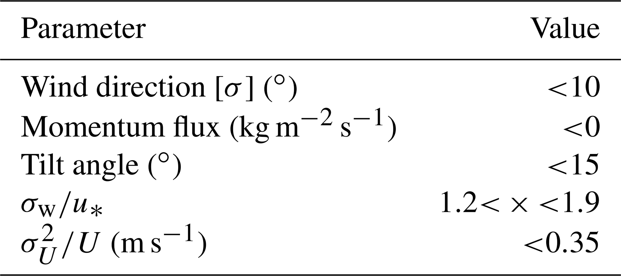
Table A3Fresh water solubility (Hcp), solubility temperature dependence () and molar volume (Vb) used in calculations of seawater solubility and Schmidt number at ambient temperature and salinity. Hcp and for freshwater are updated from Sander (2015) and Burkholder et al. (2015).
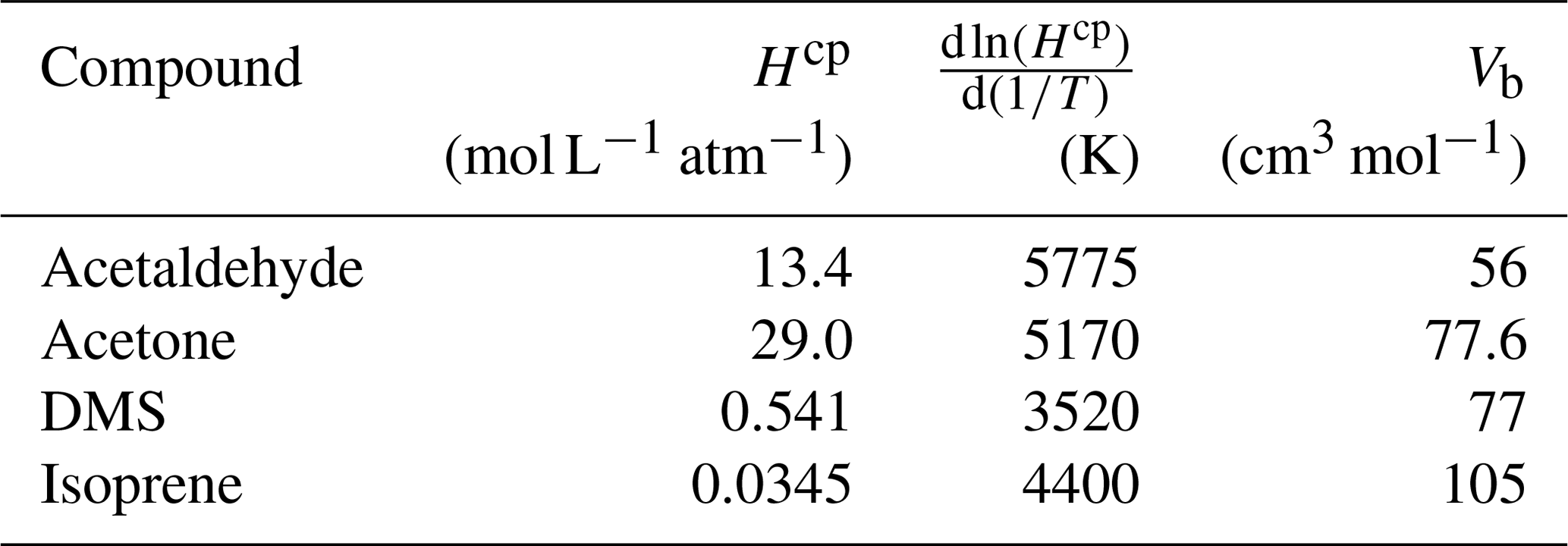
Table A4Seawater concentrations of VOCs at the L4 marine station at 2 m depth. * Denotes concentration used for two-layer calculation.
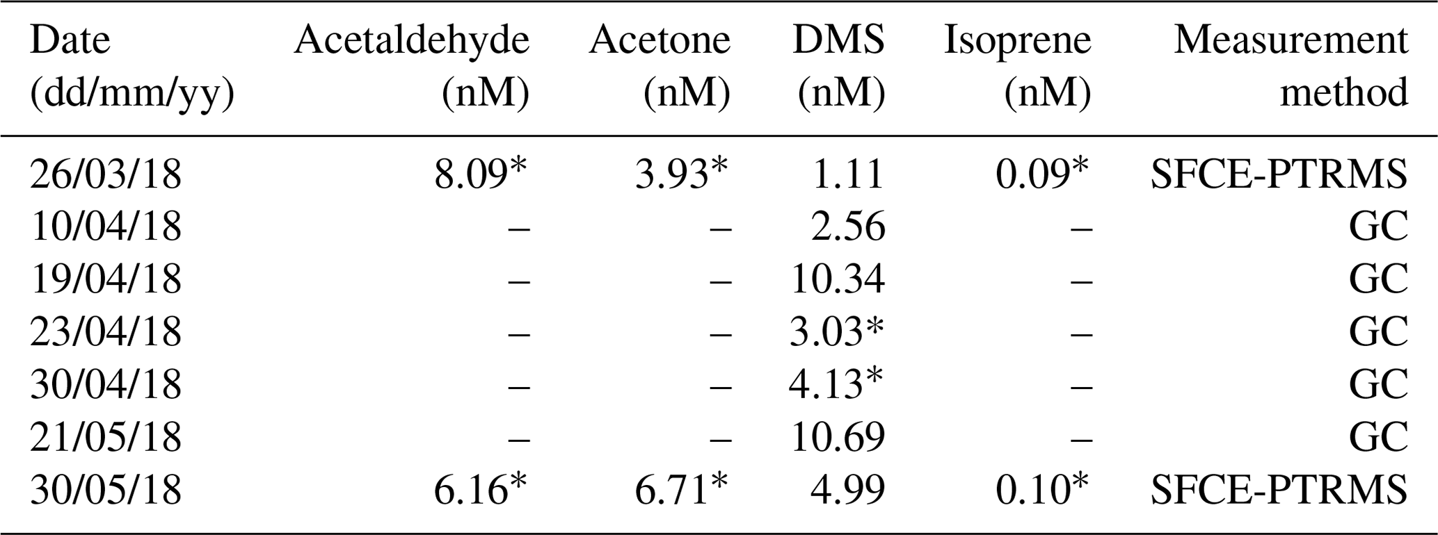
Table A3 shows the solubility and solubility temperature dependence (Burkholder et al., 2015) and molar volume data (Johnson, 2010) used in the calculations of salinity-dependent solubility and Schmidt number. In the diffusion coefficient calculation, the original association factor of solvent (2.6) was used as recommended by Saltzman et al. (1993) for DMS.
During the period with satisfactory hourly blanking (27 April–3 May 2018), the mean (± SD) L4 water temperature and salinity were 10.6 ± 0.8 ∘C and 34.9 ± 0.1 PSU. These were taken from the surface measurement of a weekly CTD profile collected on the RV Plymouth Quest. Mean atmospheric pressure was 1006 ± 4 mB, wind speed at 10 m height was 9.93 ± 3.76 m s−1 and friction velocity (also from EC) was 0.364 ± 0.166 m s−1. Table A4 shows the available VOC concentration data just before, during and after the campaign. Simultaneous measurements and calculated fluxes were made using concentration data from as close as possible to the period with satisfactory blanking (*).
Figure S2 shows the double wind rotation tilt angle correction and drag coefficient () for 10 min segments of wind data averaged into wind direction bins. The 10 min data were filtered (U>3 m s−1) to reduce the influence of the flux footprint overlapping with the narrow strip of land upwind under low wind speed conditions (Yang et al., 2019a). The majority of winds had a positive tilt angle due the rotation of ocean (horizontal) winds hitting the headland. However winds from 260–360∘ N were negatively angled due to the raised headland behind the observatory. The 30–70 and 180–240∘ N zones exhibit a small, positive tilt angle and a low drag coefficient, as might be expected for the open ocean (Kara et al., 2007; Edson et al., 2013). We define these as our two air–water exchange sectors.
Data from the Western Channel Observatory are found at http://www.westernchannelobservatory.org.uk/, last access: 20 May 2020. Additional data can be requested from the corresponding authors.
The supplement related to this article is available online at: https://doi.org/10.5194/acp-21-10111-2021-supplement.
DPP, TGB and MY designed and set up the experiment at the Penlee Point Atmospheric Observatory. MY provided eddy covariance calculation code, and DPP undertook the analysis. FEH and CW provided the seawater concentrations. DPP prepared the manuscript with contributions from all authors.
The authors declare that they have no conflict of interest.
Publisher's note: Copernicus Publications remains neutral with regard to jurisdictional claims in published maps and institutional affiliations.
The first author would like to thank fellow authors and staff at PML for assistance in transporting equipment to the observatory. Thanks are given to Rachael Beale (PML) for her L4 time series and AMT19 data that enabled a quantitative discussion and analysis with our resolved fluxes. A further thank you is expressed to the anonymous referees who gave their time to provide helpful comments that improved the presentation and discussion of the work. This is contribution 10 from the Penlee Point Atmospheric Observatory.
This work was supported by the Natural Environment Research Council and EnvEast DTP (grant no. NE/L002582/1).
This paper was edited by Neil Harris and reviewed by two anonymous referees.
Andreae, M. O., Ferek, R. J., Bermond, F., Byrd, K. P., Engstrom, R. T., Hardin, S., Houmere, P. D., LeMarrec, F., Raemdonck, H., and Chatfield, R. B.: Dimethyl sulfide in the marine atmosphere, J. Geophys. Res., 90, 12891, https://doi.org/10.1029/JD090iD07p12891, 1985.
Archer, S. D., Cummings, D. G., Llewellyn, C. A., and Fishwick, J. R.: Phytoplankton taxa, irradiance and nutrient availability determine the seasonal cycle of DMSP in temperate shelf seas, Mar. Ecol. Prog. Ser., 394, 111–124, https://doi.org/10.3354/meps08284, 2009.
Arnold, S. R., Spracklen, D. V., Williams, J., Yassaa, N., Sciare, J., Bonsang, B., Gros, V., Peeken, I., Lewis, A. C., Alvain, S., and Moulin, C.: Evaluation of the global oceanic isoprene source and its impacts on marine organic carbon aerosol, Atmos. Chem. Phys., 9, 1253–1262, https://doi.org/10.5194/acp-9-1253-2009, 2009.
Atkinson, R.: Atmospheric chemistry of VOCs and NOx, Atmos. Environ., 34, 2063–2101, https://doi.org/10.1016/S1352-2310(99)00460-4, 2000.
Atkinson, R. and Arey, J.: Atmospheric Degradation of Volatile Organic Compounds, Chem. Rev., 103, 4605–4638, https://doi.org/10.1021/cr0206420, 2003.
Baker, A. R., Turner, S. M., Broadgate, W. J., Thompson, A., McFiggans, G. B., Vesperini, O., Nightingal, P. D., Liss, P. S., and Jickells, T. D.: Distribution and sea-air fluxes of biogenic trace gases in the eastern Atlantic Ocean, Global Biogeochem. Cy., 14, 871–886, https://doi.org/10.1029/1999GB001219, 2000.
Bauer, J. E., Cai, W. J., Raymond, P. A., Bianchi, T. S., Hopkinson, C. S., and Regnier, P. A. G.: The changing carbon cycle of the coastal ocean, Nature, 504, 61–70, https://doi.org/10.1038/nature12857, 2013.
Beale, R., Dixon, J. L., Arnold, S. R., Liss, P. S., and Nightingale, P. D.: Methanol, acetaldehyde, and acetone in the surface waters of the Atlantic Ocean, J. Geophys. Res.-Ocean., 118, 5412–5425, https://doi.org/10.1002/jgrc.20322, 2013.
Beale, R., Dixon, J. L., Smyth, T. J., and Nightingale, P. D.: Annual study of oxygenated volatile organic compounds in UK shelf waters, Mar. Chem., 171, 96–106, https://doi.org/10.1016/j.marchem.2015.02.013, 2015.
Bell, T. G., de Bruyn, W. J., Miller, S. D., Ward, B., Christensen, K., and Saltzman, E. S.: Air-sea dimethylsulfide (DMS) gas transfer in the North Atlantic: Evidence for limited interfacial gas exchange at high wind speed, Atmos. Chem. Phys., 13, 11073–11087, https://doi.org/10.5194/acp-13-11073-2013, 2013.
Bell, T. G., Landwehr, S., Miller, S. D., De Bruyn, W. J., Callaghan, A. H., Scanlon, B., Ward, B., Yang, M., and Saltzman, E. S.: Estimation of bubble-mediated air-sea gas exchange from concurrent DMS and CO2 transfer velocities at intermediate-high wind speeds, Atmos. Chem. Phys., 17, 9019–9033, https://doi.org/10.5194/acp-17-9019-2017, 2017.
Blando, J. D. and Turpin, B. J.: Secondary organic aerosol formation in cloud and fog droplets: A literature evaluation of plausibility, Atmos. Environ., 34, 1623–1632, https://doi.org/10.1016/S1352-2310(99)00392-1, 2000.
Blitz, M. A., Heard, D. E., Pilling, M. J., Arnold, S. R., and Chipperfield, M. P.: Pressure and temperature-dependent quantum yields for the photodissociation of acetone between 279 and 327.5 nm, Geophys. Res. Lett., 31, 1–5, https://doi.org/10.1029/2003gl018793, 2004.
Blomquist, B. W., Fairall, C. W., Huebert, B. J., Kieber, D. J., and Westby, G. R.: DMS sea-air transfer velocity: Direct measurements by eddy covariance amd parameterizarion based on the NOAA/COAREgas transfer model, Geophys. Res. Lett., 33, 2–5, https://doi.org/10.1029/2006GL025735, 2006.
Blomquist, B. W., Huebert, B. J., Fairall, C. W., and Faloona, I. C.: Determining the sea-air flux of dimethylsulfide by eddy correlation using mass spectrometry, Atmos. Meas. Tech., 3, 1–20, https://doi.org/10.5194/amt-3-1-2010, 2010.
Blomquist, B. W., Brumer, S. E., Fairall, C. W., Huebert, B. J., Zappa, C. J., Brooks, I. M., Yang, M., Bariteau, L., Prytherch, J., Hare, J. E., Czerski, H., Matei, A., and Pascal, R. W.: Wind Speed and Sea State Dependencies of Air-Sea Gas Transfer: Results From the High Wind Speed Gas Exchange Study (HiWinGS), J. Geophys. Res.-Ocean., 122, 8034–8062, https://doi.org/10.1002/2017JC013181, 2017.
Booge, D., Marandino, C. A., Schlundt, C., Palmer, P. I., Schlundt, M., Atlas, E. L., Bracher, A., Saltzman, E. S., and Wallace, D. W. R.: Can simple models predict large-scale surface ocean isoprene concentrations?, Atmos. Chem. Phys., 16, 11807–11821, https://doi.org/10.5194/acp-16-11807-2016, 2016.
Booge, D., Schlundt, C., Bracher, A., Endres, S., Zäncker, B., and Marandino, C. A.: Marine isoprene production and consumption in the mixed layer of the surface ocean – a field study over two oceanic regions, Biogeosciences, 15, 649–667, https://doi.org/10.5194/bg-15-649-2018, 2018.
Borges, A. V., Vanderborght, J. P., Schiettecatte, L. S., Gazeau, F., Ferrón-Smith, S., Delille, B., and Frankignoulle, M.: Variability of the gas transfer velocity of CO2 in a macrotidal estuary (the Scheldt), Estuaries, 27, 593–603, https://doi.org/10.1007/BF02907647, 2004.
Borges, A. V., Delille, B., and Frankignoulle, M.: Budgeting sinks and sources of CO2 in the coastal ocean: Diversity of ecosystem counts, Geophys. Res. Lett., 32, 1–4, https://doi.org/10.1029/2005GL023053, 2005.
Broadgate, W. J., Liss, P. S., and Penkett, S. A.: Seasonal emissions of isoprene and other reactive hydrocarbon gases from the ocean, Geophys. Res. Lett., 24, 2675–2678, https://doi.org/10.1029/97GL02736, 1997.
Broadgate, W. J., Malin, G., Küpper, F. C., Thompson, A., and Liss, P. S.: Isoprene and other non-methane hydrocarbons from seaweeds: A source of reactive hydrocarbons to the atmosphere, Mar. Chem., 88, 61–73, https://doi.org/10.1016/j.marchem.2004.03.002, 2004.
Burkholder, J. B., Sander, S. P., Abbatt, J., Barker, J. R., Huie, R. E., Kolb, C. E., Kurylo, M. J., Orkin, V. L., Wilmouth, D. M., and Wine, P. H.: Chemical Kinetics and Photochemical Data for Use in Atmospheric Studies, Evaluation No. 18, JPL Publ, available at: https://jpldataeval.jpl.nasa.gov/ (last access: 10 March 2020), 2015.
Carslaw, N., Bell, N., Lewis, A. C., McQuaid, J. B., and Pilling, M. J.: A detailed case study of isoprene chemistry during the EASE96 Mace Head campaign, Atmos. Environ., 34, 2827–2836, https://doi.org/10.1016/S1352-2310(00)00088-1, 2000.
Charlson, R. J., Lovelock, J. E., Andreae, M. O., and Warren, S. G.: Oceanic phytoplankton, atmospheric sulphur, cloud albedo and climate, Nature, 326, 655–661, https://doi.org/10.1038/326655a0, 1987.
Ciuraru, R., Fine, L., Pinxteren, M. Van, D'Anna, B., Herrmann, H., and George, C.: Unravelling New Processes at Interfaces: Photochemical Isoprene Production at the Sea Surface, Environ. Sci. Technol., 49, 13199–13205, https://doi.org/10.1021/acs.est.5b02388, 2015.
Cloern, J. E., Foster, S. Q., and Kleckner, A. E.: Phytoplankton primary production in the world's estuarine-coastal ecosystems, Biogeosciences, 11, 2477–2501, https://doi.org/10.5194/bg-11-2477-2014, 2014.
Dani, K. G. S. and Loreto, F.: Trade-Off Between Dimethyl Sulfide and Isoprene Emissions from Marine Phytoplankton, Trends Plant Sci., 22, 361–372, https://doi.org/10.1016/j.tplants.2017.01.006, 2017.
de Bruyn, W. J., Clark, C. D., Pagel, L., and Singh, H.: Loss rates of acetone in filtered and unfiltered coastal seawater, Mar. Chem., 150, 39–44, https://doi.org/10.1016/j.marchem.2013.01.003, 2013.
de Bruyn, W. J., Clark, C. D., Senstad, M., Barashy, O., and Hok, S.: The biological degradation of acetaldehyde in coastal seawater, Mar. Chem., 192, 13–21, https://doi.org/10.1016/j.marchem.2017.02.008, 2017.
Dixon, J. L., Beale, R., and Nightingale, P. D.: Production of methanol, acetaldehyde, and acetone in the Atlantic Ocean, Geophys. Res. Lett., 40, 4700–4705, https://doi.org/10.1002/grl.50922, 2013.
Dixon, J. L., Beale, R., Sargeant, S. L., Tarran, G. A., and Nightingale, P. D.: Microbial acetone oxidation in coastal seawater, Front. Microbiol., 5, 1–9, https://doi.org/10.3389/fmicb.2014.00243, 2014.
Edson, J. B., Jampana, V., Weller, R. A., Bigorre, S. P., Plueddemann, A. J., Fairall, C. W., Miller, S. D., Mahrt, L., Vickers, D., and Hersbach, H.: On the exchange of momentum over the open ocean, J. Phys. Oceanogr., 43, 1589–1610, https://doi.org/10.1175/JPO-D-12-0173.1, 2013.
Exton, D. A., Suggett, D. J., McGenity, T. J., and Steinke, M.: Chlorophyll-normalized isoprene production in laboratory cultures of marine microalgae and implications for global models, Limnol. Oceanogr., 58, 1301–1311, https://doi.org/10.4319/lo.2013.58.4.1301, 2013.
Fischer, E. V., Jacob, D. J., Millet, D. B., Yantosca, R. M., and Mao, J.: The role of the ocean in the global atmospheric budget of acetone, Geophys. Res. Lett., 39, 3–7, https://doi.org/10.1029/2011GL050086, 2012.
Guenther, A. B., Karl, T. R., Harley, P., Wiedinmyer, C., Palmer, P. I., and Geron, C.: Estimates of global terrestrial isoprene emissions using MEGAN (Model of Emissions of Gases and Aerosols from Nature), Atmos. Chem. Phys., 6, 3181–3210, https://doi.org/10.5194/acp-6-3181-2006, 2006.
Hackenberg, S. C., Andrews, S. J., Airs, R., Arnold, S. R., Bouman, H. A., Brewin, R. J. W., Chance, R. J., Cummings, D., Dall'Olmo, G., Lewis, A. C., Minaeian, J. K., Reifel, K. M., Small, A., Tarran, G. A., Tilstone, G. H., and Carpenter, L. J.: Potential controls of isoprene in the surface ocean, Global Biogeochem. Cy., 31, 644–662, https://doi.org/10.1002/2016GB005531, 2017.
Halsey, K. H., Giovannoni, S. J., Graus, M., Zhao, Y., Landry, Z., Thrash, J. C., Vergin, K. L., and De Gouw, J. A.: Biological cycling of volatile organic carbon by phytoplankton and bacterioplankton, Limnol. Oceanogr., 62, 2650–2661, https://doi.org/10.1002/lno.10596, 2017.
Heald, C. L., Goldstein, A. H., Allan, J. D., Aiken, A. C., Apel, E. C., Atlas, E. L., Baker, A. K., Bates, T. S., Beyersdorf, A. J., Blake, D. R., Campos, T., Coe, H., Crounse, J. D., DeCarlo, P. F., De Gouw, J. A., Dunlea, E. J., Flocke, F. M., Fried, A., Goldan, P. D., Griffin, R. J., Herndon, S. C., Holloway, J. S., Holzinger, R., Jimenez, J. L., Junkermann, W., Kuster, W. C., Lewis, A. C., Meinardi, S., Millet, D. B., Onasch, T., Polidori, A., Quinn, P. K., Riemer, D. D., Roberts, J. M., Salcedo, D., Sive, B., Swanson, A. L., Talbot, R., Warneke, C., Weber, R. J., Weibring, P., Wennberg, P. O., Worsnop, D. R., Wittig, A. E., Zhang, R., Zheng, J., and Zheng, W.: Total observed organic carbon (TOOC) in the atmosphere: A synthesis of North American observations, Atmos. Chem. Phys., 8, 2007–2025, https://doi.org/10.5194/acp-8-2007-2008, 2008.
Henze, D. K. and Seinfeld, J. H.: Global secondary organic aerosol from isoprene oxidation, Geophys. Res. Lett., 33, 6–9, https://doi.org/10.1029/2006GL025976, 2006.
Hopkins, F. E. and Archer, S. D.: Consistent increase in dimethyl sulfide (DMS) in response to high CO2 in five shipboard bioassays from contrasting NW European waters, Biogeosciences, 11, 4925–4940, https://doi.org/10.5194/bg-11-4925-2014, 2014.
Horowitz, L. W., Walters, S., Mauzerall, D. L., Emmons, L. K., Rasch, P. J., Granier, C., Tie, X., Lamarque, J. F., Schultz, M. G., Tyndall, G. S., Orlando, J. J., and Brasseur, G. P.: A global simulation of tropospheric ozone and related tracers: Description and evaluation of MOZART, version 2, J. Geophys. Res.-Atmos., 108, 4784, https://doi.org/10.1029/2002jd002853, 2003.
Huebert, B. J., Blomquist, B. W., Yang, M., Archer, S. D., Nightingale, P. D., Yelland, M. J., Stephens, J., Pascal, R. W., and Moat, B. I.: Linearity of DMS transfer coefficient with both friction velocity and wind speed in the moderate wind speed range, Geophys. Res. Lett., 37, L01605, https://doi.org/10.1029/2009GL041203, 2010.
Hyson, P., Garratt, J. R., and Francey, R. J.: Algebraic and Electronic Corrections of Measured uw Covariance in the Lower Atmosphere, J. Appl. Meteorol., 16, 43–47, https://doi.org/10.1175/1520-0450(1977)016<0043:AAECOM>2.0.CO;2, 1977.
Jacob, D. J., Field, B. D., Jin, E. M., Bey, I., Li, Q., Logan, J. A., Yantosca, R. M., and Singh, H. B.: Atmospheric budget of acetone, J. Geophys. Res.-Atmos., 107, 4100, https://doi.org/10.1029/2001JD000694, 2002.
Johnson, M. T.: A numerical scheme to calculate temperature and salinity dependent air-water transfer velocities for any gas, Ocean Sci., 6, 913–932, https://doi.org/10.5194/os-6-913-2010, 2010.
Kaimal, J., Wyngaard, J., Izumi, Y., and Cote, O.: Spectral characteristics of surface-layer turbulence, Q. J. R. Meteorol. Soc., 098, 563–589, https://doi.org/10.1256/smsqj.41706, 1972.
Kara, A. B., Metzger, E. J., and Bourassa, M. A.: Ocean current and wave effects on wind stress drag coefficient over the global ocean, Geophys. Res. Lett., 34, 2–5, https://doi.org/10.1029/2006GL027849, 2007.
Kesselmeier, J. and Staudt, M.: Biogenic Volatile Organic Compound (VOC): An Overview on Emissions, Physiology and Ecology, J. Atmos. Chem., 33, 23–88, https://doi.org/10.1023/A:1006127516791, 1999.
Khan, M. A. H., Cooke, M. C., Utembe, S. R., Archibald, A. T., Maxwell, P., Morris, W. C., Xiao, P., Derwent, R. G., Jenkin, M. E., Percival, C. J., Walsh, R. C., Young, T. D. S., Simmonds, P. G., Nickless, G., O'Doherty, S., and Shallcross, D. E.: A study of global atmospheric budget and distribution of acetone using global atmospheric model STOCHEM-CRI, Atmos. Environ., 112, 269–277, https://doi.org/10.1016/j.atmosenv.2015.04.056, 2015.
Kieber, R. J., Zhou, X., and Mopper, K.: Formation of carbonyl compounds from UV-induced photodegradation of humic substances in natural waters: Fate of riverine carbon in the sea, Limnol. Oceanogr., 35, 1503–1515, https://doi.org/10.4319/lo.1990.35.7.1503, 1990.
Kiene, R. P., Linn, L. J., and Bruton, J. A.: New and important roles for DMSP in marine microbial communities, J. Sea Res., 43, 209–224, https://doi.org/10.1016/S1385-1101(00)00023-X, 2000.
Kim, M. J., Novak, G. A., Zoerb, M. C., Yang, M., Blomquist, B. W., Huebert, B. J., Cappa, C. D., and Bertram, T. H.: Air-Sea exchange of biogenic volatile organic compounds and the impact on aerosol particle size distributions, Geophys. Res. Lett., 44, 3887–3896, https://doi.org/10.1002/2017GL072975, 2017.
Lana, A., Bell, T. G., Simó, R., Vallina, S. M., Ballabrera-Poy, J., Kettle, A. J., Dachs, J., Bopp, L., Saltzman, E. S., Stefels, J., Johnson, J. E., and Liss, P. S.: An updated climatology of surface dimethlysulfide concentrations and emission fluxes in the global ocean, Global Biogeochem. Cy., 25, 1–17, https://doi.org/10.1029/2010GB003850, 2011.
Lewis, A. C., Carpenter, L. J., and Pilling, M. J.: Nonmethane hydrocarbons in Southern Ocean boundary layer air, J. Geophys. Res.-Atmos., 106, 4987–4994, https://doi.org/10.1029/2000JD900634, 2001.
Lewis, A. C., Hopkins, J. R., Carpenter, L. J., Stanton, J., Read, K. A., and Pilling, M. J.: Sources and sinks of acetone, methanol, and acetaldehyde in North Atlantic marine air, Atmos. Chem. Phys., 5, 1963–1974, https://doi.org/10.5194/acp-5-1963-2005, 2005.
Li, M., Karu, E., Brenninkmeijer, C. A. M., Fischer, H., Lelieveld, J., and Williams, J.: Tropospheric OH and stratospheric OH and Cl concentrations determined from CH4, CH3Cl, and SF6 measurements, Clim. Atmos. Sci., 1, 29, https://doi.org/10.1038/s41612-018-0041-9, 2018.
Liss, P. S. and Slater, P. G.: Flux of Gases across the Air-Sea Interface, Nature, 247, 181–184, https://doi.org/10.1038/247181a0, 1974.
Loades, D. C., Yang, M., Bell, T. G., Vaughan, A. R., Pound, R. J., Metzger, S., Lee, J. D., and Carpenter, L. J.: Ozone deposition to a coastal sea: comparison of eddy covariance observations with reactive air–sea exchange models, Atmos. Meas. Tech., 13, 6915–6931, https://doi.org/10.5194/amt-13-6915-2020, 2020.
Mackay, D. and Yeun, A. T. K.: Mass Transfer Coefficient Correlations for Volatilization of Organic Solutes from Water, Environ. Sci. Technol., 17, 211–217, https://doi.org/10.1021/es00110a006, 1983.
Marandino, C. A., de Bruyn, W. J., Miller, S. D., Prather, M. J., and Saltzman, E. S.: Oceanic uptake and the global atmospheric acetone budget, Geophys. Res. Lett., 32, L15806, https://doi.org/10.1029/2005GL023285, 2005.
Millet, D. B., Guenther, A. B., Siegel, D. A., Nelson, N. B., Singh, H. B., De Gouw, J. A., Warneke, C., Williams, J., Eerdekens, G., Sinha, V., Karl, T. R., Flocke, F., Apel, E. C., Riemer, D. D., Palmer, P. I., and Barkley, M.: Global atmospheric budget of acetaldehyde: 3-D model analysis and constraints from in-situ and satellite observations, Atmos. Chem. Phys., 10, 3405–3425, https://doi.org/10.5194/acp-10-3405-2010, 2010.
Moore, R. M., Oram, D. E., and Penkett, S. A.: Production of isoprene by marine phytoplankton cultures, Geophys. Res. Lett., 21, 2507–2510, https://doi.org/10.1029/94GL02363, 1994.
Nightingale, P. D., Malin, G., Law, C. S., Watson, A. J., Liss, P. S., Liddicoat, M. I., Boutin, J., and Upstill-Goddard, R. C.: In situ evaluation of air-sea gas exchange parameterizations using novel conservative and volatile tracers, Global Biogeochem. Cy., 14, 373–387, https://doi.org/10.1029/1999GB900091, 2000.
Palmer, P. I. and Shaw, S. L.: Quantifying global marine isoprene fluxes using MODIS chlorophyll observations, Geophys. Res. Lett., 32, 1–5, https://doi.org/10.1029/2005GL022592, 2005.
Quinn, P. K., Bates, T. S., Coffman, D. J., Upchurch, L., Johnson, J. E., Moore, R., Ziemba, L., Bell, T. G., Saltzman, E. S., Graff, J., and Behrenfeld, M. J.: Seasonal Variations in Western North Atlantic Remote Marine Aerosol Properties, J. Geophys. Res.-Atmos., 124, 14240–14261, https://doi.org/10.1029/2019JD031740, 2019.
Rolph, G., Stein, A., and Stunder, B.: Real-time Environmental Applications and Display sYstem: READY, Environ. Model. Softw., 95, 210–228, https://doi.org/10.1016/j.envsoft.2017.06.025, 2017.
Royer, S. J., Galí, M., Mahajan, A. S., Ross, O. N., Pérez, G. L., Saltzman, E. S., and Simó, R.: A high-resolution time-depth view of dimethylsulphide cycling in the surface sea, Sci. Rep., 6, 1–13, https://doi.org/10.1038/srep32325, 2016.
Saltzman, E. S., King, D. B., Holmen, K., and Leck, C.: Experimental determination of the diffusion coefficient of dimethylsulfide in water, J. Geophys. Res., 98, 481–486, https://doi.org/10.1029/93jc01858, 1993.
Sander, R.: Compilation of Henry's law constants (version 4.0) for water as solvent, Atmos. Chem. Phys., 15, 4399–4981, https://doi.org/10.5194/acp-15-4399-2015, 2015.
Schlundt, C., Tegtmeier, S., Lennartz, S. T., Bracher, A., Cheah, W., Krüger, K., Quack, B., and Marandino, C. A.: Oxygenated volatile organic carbon in the western Pacific convective center: Ocean cycling, air-sea gas exchange and atmospheric transport, Atmos. Chem. Phys., 17, 10837–10854, https://doi.org/10.5194/acp-17-10837-2017, 2017.
Schwarz, K., Filipiak, W., and Amann, A.: Determining concentration patterns of volatile compounds in exhaled breath by PTR-MS, J. Breath Res., 3, 027002, https://doi.org/10.1088/1752-7155/3/2/027002, 2009.
Shaw, S. L., Chisholm, S. W., and Prinn, R. G.: Isoprene production by Prochlorococcus, a marine cyanobacterium, and other phytoplankton, Mar. Chem., 80, 227–245, https://doi.org/10.1016/S0304-4203(02)00101-9, 2003.
Spirig, C., Neftel, A., Ammann, C., Dommen, J., Grabmer, W., Thielmann, A., Schaub, A., Beauchamp, J. L., Wisthaler, A., and Hansel, A.: Eddy covariance flux measurements of biogenic VOCs during ECHO 2003 using proton transfer reaction mass spectrometry, Atmos. Chem. Phys., 5, 465–481, https://doi.org/10.5194/acp-5-465-2005, 2005.
Stein, A. F., Draxler, R. R., Rolph, G. D., Stunder, B. J. B., Cohen, M. D., and Ngan, F.: Noaa's hysplit atmospheric transport and dispersion modeling system, Bull. Am. Meteorol. Soc., 96, 2059–2077, https://doi.org/10.1175/BAMS-D-14-00110.1, 2015.
Tanner, C. B. and Thurtell, G. W.: Anemoclinometer measurements of Reynolds stress and heat transport in the atmospheric surface layer, University of Wisconsin Tech. Rep., ECOM-66-G22-F, 82 pp., 1969.
Uncles, R. J., Stephens, J. A., and Harris, C.: Physical processes in a coupled bay-estuary coastal system: Whitsand Bay and Plymouth Sound, Prog. Oceanogr., 137, 360–384, https://doi.org/10.1016/j.pocean.2015.04.019, 2015.
Upstill-Goddard, R. C.: Air-sea gas exchange in the coastal zone, Estuar. Coast. Shelf Sci., 70, 388–404, https://doi.org/10.1016/j.ecss.2006.05.043, 2006.
Veres, P. R., Andrew Neuman, J., Bertram, T. H., Assaf, E., Wolfe, G. M., Williamson, C. J., Weinzierl, B., Tilmes, S., Thompson, C. R., Thames, A. B., Schroder, J. C., Saiz-Lopez, A., Rollins, A. W., Roberts, J. M., Price, D., Peischl, J., Nault, B. A., Møller, K. H., Miller, D. O., Meinardi, S., Li, Q., Lamarque, J. F., Kupc, A., Kjaergaard, H. G., Kinnison, D., Jimenez, J. L., Jernigan, C. M., Hornbrook, R. S., Hills, A., Dollner, M., Day, D. A., Cuevas, C. A., Campuzano-Jost, P., Burkholder, J. B., Paul Bui, T., Brune, W. H., Brown, S. S., Brock, C. A., Bourgeois, I., Blake, D. R., Apel, E. C., and Ryerson, T. B.: Global airborne sampling reveals a previously unobserved dimethyl sulfide oxidation mechanism in the marine atmosphere, P. Natl. Acad. Sci. USA, 117, 4505–4510, https://doi.org/10.1073/pnas.1919344117, 2020.
Wang, S., Hornbrook, R. S., Hills, A., Emmons, L. K., Tilmes, S., Lamarque, J. F., Jimenez, J. L., Campuzano-Jost, P., Nault, B. A., Crounse, J. D., Wennberg, P. O., Kim, M., Allen, H. M., Ryerson, T. B., Thompson, C. R., Peischl, J., Moore, F., Nance, D., Hall, B., Elkins, J., Tanner, D., Huey, L. G., Hall, S. R., Ullmann, K., Orlando, J. J., Tyndall, G. S., Flocke, F. M., Ray, E., Hanisco, T. F., Wolfe, G. M., St. Clair, J., Commane, R., Daube, B., Barletta, B., Blake, D. R., Weinzierl, B., Dollner, M., Conley, A., Vitt, F., Wofsy, S. C., Riemer, D. D., and Apel, E. C.: Atmospheric Acetaldehyde: Importance of Air-Sea Exchange and a Missing Source in the Remote Troposphere, Geophys. Res. Lett., 46, 5601–5613, https://doi.org/10.1029/2019GL082034, 2019.
Wang, S., Apel, E. C., Schwantes, R., Bates, K., Jacob, D., Fischer, E., Hornbrook, R. S., Hills, A., Emmons, L., Pan, L., Honomichl, S., Tilmes, S., Lamarque, J., Yang, M., Marandino, C., Saltzman, E., Bruyn, W., Kameyama, S., Tanimoto, H., Omori, Y., Hall, S., Ullmann, K., Ryerson, T., Thompson, C., Peischl, J., Daube, B., Commane, R., McKain, K., Sweeney, C., Thames, A., Miller, D., Brune, W. H., Diskin, G., DiGangi, J., and Wofsy, S.: Global Atmospheric Budget of Acetone: Air-Sea Exchange and the Contribution to Hydroxyl Radicals, J. Geophys. Res.-Atmos., 2, 1–23, https://doi.org/10.1029/2020JD032553, 2020a.
Wang, W.-L., Song, G., Primeau, F., Saltzman, E. S., Bell, T. G., and Moore, J. K.: Global ocean dimethyl sulfide climatology estimated from observations and an artificial neural network, Biogeosciences, 17, 5335–5354, https://doi.org/10.5194/bg-17-5335-2020, 2020b.
Warneck, P. and Moortgat, G. K.: Quantum yields and photodissociation coefficients of acetaldehyde in the troposphere, Atmos. Environ., 62, 153–163, https://doi.org/10.1016/j.atmosenv.2012.08.024, 2012.
Warneke, C., De Gouw, J. A., Kuster, W. C., Goldan, P. D., and Fall, R.: Validation of atmospheric VOC measurements by proton-transfer-reaction mass spectrometry using a gas-chromatographic preseparation method, Environ. Sci. Technol., 37, 2494–2501, https://doi.org/10.1021/es026266i, 2003.
Williams, J., Holzinger, R., Gros, V., Xu, X., Atlas, E. L., and Wallace, D. W. R.: Measurements of organic species in air and seawater from the tropical Atlantic, Geophys. Res. Lett., 31, 1–5, https://doi.org/10.1029/2004GL020012, 2004.
Wofsy, S. C., Afshar, S., Allen, H. M., Apel, E. C., Asher, E. C., Barletta, B., Bent, J., Bian, H., Biggs, B. C., Blake, D. R., Blake, N., Bourgeois, I., Brock, C. A., Brune, W. H., Budney, J. W., Bui, T. P., Butler, A., Campuzano-Jost, P., Chang, C. S., Chin, M., Commane, R., Correa, G., Crounse, J. D., Cullis, P. D., Daube, B. C., Day, D. A., Dean-Day, J. M., Dibb, J. E., DiGangi, J. P., Diskin, G. S., Dollner, M., Elkins, J. W., Erdesz, F., Fiore, A. M., Flynn, C. M., Froyd, K. D., Gesler, D. W., Hall, S. R., Hanisco, T. F., Hannun, R. A., Hills, A. J., Hintsa, E. J., Hoffman, A., Hornbrook, R. S., Huey, L. G., Hughes, S., Jimenez, J. L., Johnson, B. J., Katich, J. M., Keeling, R. F., Kim, M. J., Kupc, A., Lait, L. R., Lamarque, J.-F., Liu, J., McKain, K., Mclaughlin, R. J., Meinardi, S., Miller, D. O., Montzka, S. A., Moore, F. L., Morgan, E. J., Murphy, D. M., Murray, L. T., Nault, B. A., Neuman, J. A., Newman, P. A., Nicely, J. M., Pan, X., Paplawsky, W., Peischl, J., Prather, M. J., Price, D. J., Ray, E. A., Reeves, J. M., Richardson, M., Rollins, A. W., Rosenlof, K. H., Ryerson, T. B., Scheuer, E., Schill, G. P., Schroder, J. C., Schwarz, J. P., St.Clair, J. M., Steenrod, S. D., Stephens, B. B., Strode, S. A., Sweeney, C., Tanner, D., Teng, A. P., Thames, A. B., Thompson, C. R., Ullmann, K., Veres, P. R., Vieznor, N., Wagner, N. L., Watt, A., Weber, R., Weinzierl, B., Wennberg, P. O., Williamson, C. J., Wilson, J. C., Wolfe, G. M., Woods, C. T., and Zeng, L. H.: ATom: Merged Atmospheric Chemistry, Trace Gases, and Aerosols, ORNL DAAC [Dataset], https://doi.org/10.3334/ORNLDAAC/1581, 2018.
Wohl, C., Capelle, D., Jones, A., Sturges, W. T., Nightingale, P. D., Else, B. G. T., and Yang, M.: Segmented flow coil equilibrator coupled to a proton-transfer-reaction mass spectrometer for measurements of a broad range of volatile organic compounds in seawater, Ocean Sci., 15, 925–940, https://doi.org/10.5194/os-15-925-2019, 2019.
Wohl, C., Brown, I. J., Kitidis, V., Jones, A. E., Sturges, W. T., Nightingale, P. D., and Yang, M.: Underway seawater and atmospheric measurements of volatile organic compounds in the Southern Ocean, Biogeosciences, 17, 2593–2619, https://doi.org/10.5194/bg-17-2593-2020, 2020.
Yang, M. and Fleming, Z. L.: Estimation of atmospheric total organic carbon (TOC) – Paving the path towards carbon budget closure, Atmos. Chem. Phys., 19, 459–471, https://doi.org/10.5194/acp-19-459-2019, 2019.
Yang, M., Blomquist, B. W., Fairall, C. W., Archer, S. D., and Huebert, B. J.: Air-sea exchange of dimethylsulfide in the Southern Ocean: Measurements from so GasEx compared to temperate and tropical regions, J. Geophys. Res.-Ocean., 116, 1–17, https://doi.org/10.1029/2010JC006526, 2011a.
Yang, M., Huebert, B. J., Blomquist, B. W., Howell, S. G., Shank, L. M., McNaughton, C. S., Clarke, A. D., Hawkins, L. N., Russell, L. M., Covert, D. S., Coffman, D. J., Bates, T. S., Quinn, P. K., Zagorac, N., Bandy, A. R., de Szoeke, S. P., Zuidema, P. D., Tucker, S. C., Brewer, W. A., Benedict, K. B., and Collett, J. L.: Atmospheric sulfur cycling in the southeastern Pacific – longitudinal distribution, vertical profile, and diel variability observed during VOCALS-REx, Atmos. Chem. Phys., 11, 5079–5097, https://doi.org/10.5194/acp-11-5079-2011, 2011b.
Yang, M., Nightingale, P. D., Beale, R., Liss, P. S., Blomquist, B. W., and Fairall, C. W.: Atmospheric deposition of methanol over the Atlantic Ocean, P. Natl. Acad. Sci. USA, 110, 20034–20039, https://doi.org/10.1073/pnas.1317840110, 2013a.
Yang, M., Archer, S. D., Blomquist, B. W., Ho, D. T., Lance, V. P., and Torres, R. J.: Lagrangian evolution of DMS during the Southern Ocean gas exchange experiment: The effects of vertical mixing and biological community shift, J. Geophys. Res.-Ocean., 118, 6774–6790, https://doi.org/10.1002/2013JC009329, 2013b.
Yang, M., Beale, R., Smyth, T. J., and Blomquist, B. W.: Measurements of OVOC fluxes by eddy covariance using a proton-transfer- reaction mass spectrometer – method development at a coastal site, Atmos. Chem. Phys., 13, 6165–6184, https://doi.org/10.5194/acp-13-6165-2013, 2013c.
Yang, M., Blomquist, B. W., and Nightingale, P. D.: Air-sea exchange of methanol and acetone during HiWinGS: Estimation of air phase, water phase gas transfer velocities, J. Geophys. Res.-Ocean., 119, 7308–7323, https://doi.org/10.1002/2014JC010227, 2014a.
Yang, M., Beale, R., Liss, P. S., Johnson, M. T., Blomquist, B. W., and Nightingale, P. D.: Air–sea fluxes of oxygenated volatile organic compounds across the Atlantic Ocean, Atmos. Chem. Phys., 14, 7499–7517, https://doi.org/10.5194/acp-14-7499-2014, 2014b.
Yang, M., Bell, T. G., Hopkins, F. E., Kitidis, V., Cazenave, P. W., Nightingale, P. D., Yelland, M. J., Pascal, R. W., Prytherch, J., Brooks, I. M., and Smyth, T. J.: Air-sea fluxes of CO2 and CH4 from the penlee point atmospheric observatory on the south-west coast of the UK, Atmos. Chem. Phys., 16, 5745–5761, https://doi.org/10.5194/acp-16-5745-2016, 2016a.
Yang, M., Bell, T. G., Blomquist, B. W., Fairall, C. W., Brooks, I. M., and Nightingale, P. D.: Air-sea transfer of gas phase controlled compounds, IOP Conf. Ser. Earth Environ. Sci., 35, 012011, https://doi.org/10.1088/1755-1315/35/1/012011, 2016b.
Yang, M., Bell, T. G., Hopkins, F. E., and Smyth, T. J.: Attribution of atmospheric sulfur dioxide over the English Channel to dimethyl sulfide and changing ship emissions, Atmos. Chem. Phys., 16, 4771–4783, https://doi.org/10.5194/acp-16-4771-2016, 2016c.
Yang, M., Prytherch, J., Kozlova, E., Yelland, M. J., Parenkat Mony, D., and Bell, T. G.: Comparison of two closed-path cavity-based spectrometers for measuring air-water CO2 and CH4 fluxes by eddy covariance, Atmos. Meas. Tech., 9, 5509–5522, https://doi.org/10.5194/amt-9-5509-2016, 2016d.
Yang, M., Bell, T. G., Brown, I. J., Fishwick, J. R., Kitidis, V., Nightingale, P. D., Rees, A. P., and Smyth, T. J.: Insights from year-long measurements of air–water CH4 and CO2 exchange in a coastal environment, Biogeosciences, 16, 961–978, https://doi.org/10.5194/bg-16-961-2019, 2019a.
Yang, M., Norris, S. J., Bell, T. G., and Brooks, I. M.: Sea spray fluxes from the southwest coast of the United Kingdom-Dependence on wind speed and wave height, Atmos. Chem. Phys., 19, 15271–15284, https://doi.org/10.5194/acp-19-15271-2019, 2019b.
Zhou, S., Gonzalez, L., Leithead, A., Finewax, Z., Thalman, R., Vlasenko, A., Vagle, S., Miller, L. A., Li, S. M., Bureekul, S., Furutani, H., Uematsu, M., Volkamer, R., and Abbatt, J. P. D.: Formation of gas-phase carbonyls from heterogeneous oxidation of polyunsaturated fatty acids at the air-water interface and of the sea surface microlayer, Atmos. Chem. Phys., 14, 1371–1384, https://doi.org/10.5194/acp-14-1371-2014, 2014.
Zhou, X. and Mopper, K.: Photochemical production of low-molecular-weight carbonyl compounds in seawater and surface microlayer and their air-sea exchange, Mar. Chem., 56, 201–213, https://doi.org/10.1016/S0304-4203(96)00076-X, 1997.
Zhu, Y. and Kieber, D. J.: Wavelength- and Temperature-Dependent Apparent Quantum Yields for Photochemical Production of Carbonyl Compounds in the North Pacific Ocean, Environ. Sci. Technol., 52, 1929–1939, https://doi.org/10.1021/acs.est.7b05462, 2018.
- Abstract
- Introduction
- Method
- Results and discussion
- Conclusions
- Appendix A: Additional eddy covariance method details
- Appendix B: Two-layer flux calculation additional information
- Appendix C: Wind sector determination
- Data availability
- Author contributions
- Competing interests
- Disclaimer
- Acknowledgements
- Financial support
- Review statement
- References
- Supplement